Topological Phases, Entanglement and Boson Condensation Huan He A Dissertation Presented to the Faculty of Princeton University in Candidacy for the Degree of Doctor of Philosophy Recommended for Acceptance by the Department of Physics Adviser: Bogdan Andrei Bernevig June 2019
The F -symbol also needs to satisfy pentagon and hexagon equations, the details of
which are omitted in this dissertation.
13
Chapter 2
An Example: Toric Code Model
The toric code model and its generalizations have been extensively studied in the
literature. We will present the toric code model in different languages including the
stabilizer code, the tensor network state, the topological field theory and the modular
tensor category.
2.1 Stabilizer Code
The 2D toric code model, realizing a discrete Z2 gauge symmetry on lattice[41], is a
stabilizer code defined on any 2D random lattice. It exhibits the topological order
and supports gapped anyonic excitations. For simplicity, the 2D toric code introduced
in this section is defined on a square lattice with physical spins on all bonds of the
lattice, and the Hamiltonian consists of vertex terms and plaquette terms:
H = −∑v
Av −∑p
Bp. (2.1)
14
Z Z
x
x
xx
x
y
Z
Z
(a) (b)
Figure 2.1: The Hamiltonian terms of the 2D toric code model. Panel (a) is Av whichis a product of 4 Z operators around the vertex v, and Panel (b) is Bp which is aproduct of 4 X operators around the plaquette p.
Here, Av is the product of four Pauli Z matrices around a vertex v and Bp is the
product of four Pauli X matrices around a plaquette p.
Av =∏i∈v
Zi, Bp =∏i∈p
Xi. (2.2)
These two terms are illustrated in Fig. 2.1. Note that all these operators will commute
with each other:
[Av, Av′ ] = 0, ∀ v, v′,
[Bp, Bp′ ] = 0, ∀ p, p′,
[Av, Bp] = 0, ∀ v, p.
(2.3)
Hence, the ground states of the 2D toric code model need to satisfy the constraints:
Av|GS〉 = |GS〉, Bp|GS〉 = |GS〉, (2.4)
for all vertices v and plaquettes p. Each of the eigenvalue equations is a constraint
for the ground state wave function. Note that the local Hamiltonian terms satisfy the
15
following redundancy on a closed manifold:
∏v
Av = 1,∏p
Bp = 1. (2.5)
The ground state degeneracy (GSD) satisfying Eq. (2.4) is counted as follows:
GSD =2# of qubits
2# of indep. GSD constraints=
2# of bonds
2# of vertices + # of plaquettes - 2= 22−χ (2.6)
where
χ = # of vertices + # of plaquettes - # of bonds (2.7)
is the Euler characteristic. For a torus, χ = 0. Thus the GSD on a torus is 4. The
number 2 in the exponent comes from the redundancy in Eq. (2.5). The calculation
can certainly be generalized to other manifolds, and the GSD only depends on the
Euler characteristic and hence topological.
2.2 Tensor Network State
In order to conveniently construct the TNS for the 2D toric code model, we introduce
projector g tensors on each bond of the square lattice and local T tensors on each
vertex of the square lattice. The physical or virtual index is of dimension 2 and
labeled as 0, 1. The g tensor has 1 physical index and 2 virtual indices, and the T
tensor has 4 virtual indices. The TNS is depicted in Fig. 2.2. The same construction
will be heavily used in Chapter 6.
The projector g tensor identifies the physical index with the virtual indices
gpij =
1 if p = i = j ∈ {0, 1}
0 otherwise
(2.8)
16
where p is the physical index, and i and j are thr virtual indices. The rest of the
calculations is to construct a T tensor such that the TNS satisfies Eq. (2.4) on the
TNS. We choose to directly act Av and Bp operators on the TNS. Note that g tensor
identifies the physical index and the virtual indices. The actions of X and Z Pauli
matrices on the physical indices are transferred to the virtual indices:
TZ
Z
Z
Z
Z
Z
Z
Z
g
g
g
g
g
=
Tg
gg g
x
x
x x
x xx
xx x
x
x=
. (2.9)
Tg
x
y
Figure 2.2: The TNS for the 2D toric code model on a square lattice. On each bond,we associate a projector g tensor, and on each vertex, we associate a local T tensor.The connected lines are contracted virtual indices. The lines with arrows are thephysical indices.
17
In order to implement Eq. (2.4), we require the four Pauli Z matrices (in the first
line) and two Pauli X matrices (in the second line) acting on the virtual indices in the
dashed red squares to be identity operations. Then we have two (strong) conditions
respectively:
Txx,yy = (−1)x+x+y+yTxx,yy
Txx,yy = T(1−x)x,(1−y)y = T(1−x)x,y(1−y)
= Tx(1−x),(1−y)y = Tx(1−x),y(1−y).
(2.10)
where x, x are the two indices of the T tensor in the x-direction, and the y, y are the
two indices of the T tensor in the y-direction. As a result, the local T tensors are
fixed up to an overall factor:
Txx,yy =
0 if x+ x+ y + y = 1 mod 2
1 if x+ x+ y + y = 0 mod 2.
(2.11)
Hence, we have constructed the TNS for the ground state. It is a natural question
that how to construct all degenerate ground state on a torus, since this method only
gives rise to one tensor. The solution to this puzzle is that the boundary conditions
of the TNS can be twisted in both directions without breaking the conditions in
Eq. (2.4)[30].
2.3 Modular Tensor Category
The excited states are also labeled by the eigenvalues of Av and Bp, due to the
fact that all local Hamiltonian terms commute with each other. The excited state
has eigenvalues −1 for some local Hamiltonian terms, while the ground state has all
eigenvalues 1 for all local terms. To create such excitations from the ground state, an
18
Figure 2.3: Left panel: The line operator in the first equation of Eq. (2.12). Theblue line is the path for C. Right panel: The line operator in the second equation ofEq. (2.12). The blue line is the path for C on the dual lattice. The red dots representthe excitation created. W (C) creates two excitations at the ends of C which have−1 eigenvalues of Av. W (C) creates two excitations at the ends of C which have −1eigenvalues of Bp.
observation is that line operators can be constructed as follows:
W (C) =∏i∈C
Xi, W (C) =∏i∈C
Zi, (2.12)
where C is a path on the lattice while C is a path on the dual lattice. See Fig. 2.3 for
an illustration. When the line operators act on the ground states, the Hamiltonian
terms near the two ends of the line have eigenvalues −1. If C or C is closed, then the
energy remains the same as the ground state energy. Thus the excitations are always
created by pairs. Moreover, if C or C winds around the cycles of the lattice, for
instance the two cycles of a torus, then W (C) or W (C) commutes with all the local
terms in the Hamiltonian, and cannot be generated by the local Hamiltonian terms.
Hence, these winding operators serve as good quantum numbers to distinguish the 4
ground states on torus.
The excitation, measured by an Av operator and created by W (C), is commonly
dubbed as e (charge), while the excitation, measured by an Bp operator and created by
N(NC), is dubbed as m (flux). Their composite particle is dubbed as f . Combining
the trivial particle denoted as 1, there are four excitations: 1, e, m and f . Their
19
fusion rules can be derived from their operators:
e× e = 1, m×m = 1, f × f = 1, e×m = f. (2.13)
The braiding statistics of these excitations can be derived from their operators’ com-
mutation relation. Their braiding statistics is encoded in the modular S matrix in
the basis of (1, e,m, f):
S =1
2
1 1 1 1
1 1 −1 −1
1 −1 1 1
1 −1 −1 1
(2.14)
The matrix element Sab is the braiding statistics of the anyon a and the anyon b.
Their topological spins are encoded in the modular T matrix:
T =
1 0 0 0
0 1 0 0
0 0 1 0
0 0 0 −1
(2.15)
The diagonal matrix element Taa is the topological spin for the anyon a.
The F -symbols is omitted in this dissertation since it is trivial for the toric code
model.
2.4 BF Field Theory
In this section, we show that a Z2 BF theory will reproduce the same physics as that
in the toric code Hamiltonian model. The Lagrangian for a ZN BF theory is:
L =N
2πεµνρbµ∂νaρ. (2.16)
20
For the reader who are familiar with differential forms, it is equivalent to write:
L =N
2πb ∧ da. (2.17)
Note that this Lagrangian can be casted in the form of K-matrix Chern-Simons
theory. Restricting ZN to Z2, the Lagrangian reduces to:
L =2
2πεµνρbµ∂νaρ. (2.18)
This Lagrangian exhibits the gauge symmetry as follows:
aµ 7→ aµ + ∂µα, bµ 7→ bµ + ∂µβ. (2.19)
where α and β can be any functions.
Applying canonical quantization for this gauge theory will reproduce the same
results for the toric code model. We start with gauge fixing. Tuning α and β can fix
However, θ(···σ1··· ) = −θ(···σψ··· ), implying that the restrictions of (· · ·σ, 1 · · · ) are con-
fined, because they have another lift (· · ·σ, ψ · · · ) with different topological spin. By
that argument we have shown that the set Q consisting of particles with least one
and at most N − 1 σ’s restricts only to confined particles. On the other hand, we
know that particles containing no σ’s (i.e., only 1’s or ψ’s) restrict to single deconfined
particles:
• By closure of the condensate, any particle with even number of ψ and otherwise
1 restricts to the new vacuum 1′.
• Any particle with odd number of ψ and otherwise 1 restricts to the deconfined
particle ψ′. Their fusion rule is
ψ′ × ψ′ = 1′. (3.75)
The only particle left to consider is σ(N) ≡ (σ, . . . , σ). It is easy to show that
σ(N) × Q ⊆ Q. It then follows from the a = σ(N), b ∈ Q, t = ϕ component of
Eq. (3.5) that σ(N) and particles in Q restrict to disjoint sets of particles, because
the righthand side of Eq. (3.5) is zero in this case, as none of the particles in Q
restrict to the vacuum. But then the restriction of σ(N) cannot possibly contain
confined particles as those confined particles would have just a single lift σ(N), which
57
is impossible from the definition of confined particle. Hence σ(N) restricts only to
deconfined particles, and we can identify Q as the set of lifts of all confined particles.
We can say more about the restriction of σ(N). Note DU = DA/q = 2N/2N−1 =
2, because q is equal to the number of condensed bosons i.e., q = 2N−1. As we
already know 1′, ψ′ are deconfined, DU =√
1 + 1 + . . . = 4, where . . . are additional
contributions from the restriction of σ(N). When N is not a multiple of 8, there are
just two options. Either case (1) (σ, · · · , σ) splits into just two Abelian particles
distinct from 1′, ψ′, or case (2) (σ, · · · , σ) has a single restriction with quantum
dimension√
2. (When N is a multiple of 8 the σ-string is itself a fermion or boson
and could restrict to the ψ′ and the vacuum, respectively. However, by DU = 2 it is
not possible that ψ′ and the σ-string have a common restriction in the case where N
is an odd-integer multiple of 8 (since DU =√
3 in that case). The case where N is a
multiple of 16 will be discussed separately below.) Consider now from Eq. (3.64) the
matrix element that corresponds to any particle t in the restriction of (σ, · · · , σ) and
the identity in A,
nt(σ,··· ,σ) =
√2N
2dt, (3.76)
since we know from the discussion following Eq. (3.74) that t has only one lift,
(σ, · · · , σ).
From the condition that nt(σ,··· ,σ) is integer, we conclude that case (1) applies to
even N and case (2) to odd N . We now analyze the two cases separately.
Case: N odd According to Eq. (3.76), we have (σ, · · · , σ)→ 2(N−1)/2σ′. It follows
from the fusion rules of the original theory, i.e., from Eq. (3.5) by choosing a = b =
(σ, · · · , σ), that
σ′ × σ′ = 1′ + ψ′. (3.77)
58
Thus, 1′, σ′, ψ′ furnish the same (Ising) fusion algebra as 1, σ, ψ do in every layer. The
spin factors of the deconfined restrictions are given by
θ1′ = 1, θσ′ = e2πiν/16, θψ′ = −1, (3.78)
where ν = N mod 16 is an odd integer, for N is odd. We have thus obtained all
TQFTs with Ising fusion rules that appear in Kitaev’s 16-fold way.
Case: N even If N is even, Eq. (3.76) yields the restriction (σ, · · · , σ)→ 2N/2−1a′+
2N/2−1b′ with equal coefficients. To find the fusion rules for a′ and b′, we solve
Eq. (3.64). This leaves two possibilities
a′ × a′ = b′ × b′ = 1′, a′ × b′ = ψ′, (3.79)
a′ × a′ = b′ × b′ = ψ′, a′ × b′ = 1′. (3.80)
Here, Eq. (3.79) are the toric code fusion rules. Which of the two cases applies can
be determined from the equation S2 = Θ(ST )3 = C, by using the topological spins
θa′ = θb′ = e2πiN/16. (3.81)
For N = 2 mod 4 one finds the solution Eq. (3.80) and for N = 4 mod 4 one finds
the solution Eq. (3.79).
The case where N is a multiple of 16 has to be considered separately. The con-
densation described here leads to the toric code TQFT in which a′ and b′ are bosons.
We have shown above that the toric code can be condensed to the trivial TQFT by
condensing either a′ or b′ (which were called e and m before). Thus, in the case where
the σ string is a boson, two condensations are possible: one leads to the toric code
and in the other one, in which the σ string restricts in part to the vacuum, leads to
59
the trivial TQFT. The toric code is also the TQFT that was proposed to describe a
gauged s-wave superconductor without topological edge modes. [109]
Together, this Z16 grading represents Kitaev’s 16-fold way, yielding a (non-
)Abelian fusion category for the vortices of even (odd) layer length. From the point
of view of layer construction[108], we note that ψ′ is a point-like fermionic excitation
in 3D space, while σ′, a′ and b′ are to be interpreted as vortex or line-like excitations
in 3D, because their lift has a nontrivial anyon in each layer.
It is tempting to consider the topological orders that have been proposed in
Refs. [110, 111] as the possible symmetry-preserving gapped surface terminations
of time-reversal symmetric (3+1)-dimensional superconductors as another example
of a theory with Z16 grading under condensation. The topological index ν of the
bulk superconductor has been shown to be only meaningful mod 16 in the presence
of interactions. The ν = 1 surface topological order was proposed to be nonmodular
category SO(3)6, while that for ν = 2 is the so-called T-Pfaffian state. We do not
further elaborate on possible condensations in this theory here, as the focus of the
present work is on condensation in modular categories. However, if we were to apply
the formalism of Eq. (3.64) to this problem, none of the possible condensation tran-
sitions in a double layer SO(3)6×SO(3)6 would lead to the T-Pfaffian. Rather, one
can condense all bosons in SO(3)6×SO(3)6 to obtain the trivial nonmodular TQFT
{1, f} with only one Abelian fermion f .
3.7.2 Theories with Z-fold way: Fibonacci TQFT
Not every TQFT has a Zm-graded structure under condensation. The simplest
counter-example is the Fibonacci TQFT with the single nontrivial anyon τ and the
fusion rule
τ × τ = 1 + τ. (3.82)
60
It has topological spin θτ = ei4π/5 and quantum dimension dτ = φ, where φ =
(1 +√
5)/2 is the golden ratio.
First, we want to show that no condensation is possible in 5 layers of Fibonacci,
despite the presence of the boson (τττττ). We will show that there is no matrix M
that describes a condensation and satisfies Eq. (3.48). To see this, consider the (1,b)
component of the equation MSFib(5) = SFib(5)M ,
∑a
nϕa (SFib(5))a,b =1
(2 + φ)5/2
∑a
daMa,b. (3.83)
Observe that the righthand side is nonnegative for any b. Specializing to b =
(τ, 1, 1, 1, 1), we find the lefthand side
(2 + φ)−5/2(φ− nϕ(τττττ)φ
4), (3.84)
which is negative for any nϕ(τττττ) ≥ 1, i.e., for any condensation. Therefore, no
condensation transition is possible in 5 layers of Fibonacci (see Ref. [21] for an
alternative proof).
Second, let us show further that no condensation is possible in 10 layers of Fi-
bonacci. Besides the vacuum, there is a boson with a τ anyon in every layer, which
we denote by (10τ), and 252 =(
105
)bosons with τ anyons in exactly 5 layers.
Again, we will show that there is no matrix M that describes a condensation and
satisfies Eq. (3.48). To see this, we consider the (1,b) component of the equation
MSFib(10) = SFib(10)M , but this time for the choice b = (10τ). Up to an overall factor
of the total quantum dimension, the equation reads
nϕ1φ10 +
∑a∈5τ bosons
(−1)5φ5nϕa + (−1)10nϕ(10τ)
= nϕ(10τ) +∑
a∈5τ bosons
φ5Ma,(10τ) + φ10M(10τ),(10τ).
(3.85)
61
Using nϕ1 = 1, it simplifies to
0 = φ5(M(10τ),(10τ) − 1
)+
∑a∈5τ bosons
(nϕa +Ma,(10τ)
). (3.86)
We can see that Eq. (3.86) has no nontrivial solution: Since φ5 is irrational, the first
term needs to be zero on its own, which requires M(10τ),(10τ) = 1. This implies that
(10τ) does not condense, as it has noninteger quantum dimension and would therefore
have to split in order to condense. However, the second term in Eq. (3.86) is a sum of
nonnegative numbers that can only vanish if nϕa = 0, ∀a. Hence, none of the bosons
condenses.
In fact, one can show that no condensation is possible for any number of layers N
of the Fibonacci TQFT [112]. We will reformulate this proof much more easily using
the formalism developed in this chapter elsewhere in a way that also generalizes to
other TQFTs.
Obstructions against the condensation of bosons within our formalism can only
ever occur in theories that contain non-Abelian anyons. In Abelian theories, any
potentially condensing boson J is a simple current (of order d), and one can explicitly
construct a theory in wich J is condensed as follows: Form all the orbits [a] with
respect to J , as defined in Eq. (3.30). The orbit of the identity is the condensate. If
all anyons in an orbit [a] have the same topological spin, the orbit labels a particle t[a]
in the theory U , otherwise all particles in the orbit are confined. If t[a] is unconfined,
choose nt[a]b = 1 if b ∈ [a] and n
t[a]b = 0 otherwise. Further, choose St[a],t[b] = dSa,b and
Nt[c]t[a],t[b]
=d∑
n=0
N c×Jna,b , (3.87)
for t[a], t[b], and t[c] unconfined. In can be readily shown that this choice is a consis-
tent solution to Eqs. (3.64) and (3.65) and therefore a valid condensation within our
formalism.
62
3.8 Conclusions
In summary, we derived a framework for the condensation of anyons that is applicable
to modular tensor category models of topological order. Our derivation is based
on a small number of physical assumptions and focuses on the computation of the
modular matrices S and T of the theory after condensation. Based on this, we propose
an algorithm to carry out this computation. This algorithm first seeks symmetric
nonnegative integer matrices M that commute with the modular matrices S and
T of the original theory. It then proceeds by factorizing M = nnT in a product
of a nonnegative integer matrix n with itself. Finally, the equations Sn = nS and
Tn = nT are solved. Our algorithm has proven to be practically useful in all examples
that we studied. We finally demonstrated that the equations that are central to our
derivation are powerful constraints on condensation transitions in general.
This leads us to several open problems that are not answered by the present
work. One concerns the assumption that βt = 0 for all confined particles t. We have
shown in Secs. 3.4 and 3.5 that this relation follows from weaker assumptions for
certain theories. But a general proof of this statement is lacking, so that it remains
an assumption for us. Other questions concern the uniqueness of solutions and the
transitivity of condensation transitions. For example, given an M , is there a unique
n that solves M = nnT and leads to a valid condensed theory? And given such a
solution n, is there a unique consistent solution S and T? In a similar vein, is the
condensed theory completely characterized by the coefficients nϕa?1 At present, we do
not have counterexamples against affirmative answers to these questions.
Another future direction could be the condensations in the presence of global
symmetries[105]. When we have global symmetries on top of a topologically or-
dered system, the anyons may transform in a projective representation. A direct
1Indeed, we cannot exclude the possibility that additional information, like certain vertex liftingcoefficients, are needed to fully determine the topological order of the condensed phase.
63
consequence is that certain condensations may not be able to happen if all global
symmetries are respected.
64
Chapter 4
No-Go Theorem for Boson
Condensation in Topologically
Ordered Quantum Liquids
One motivation to study condensation transitions is to classify topological order. An
important example are the 16 types of gauged chiral superconductors introduced by
Kitaev [20]. Kiteav showed that while two-dimensional superconductors are classified
by an integer Z, only 16 bulk phases are topologically distinct. This construction
can be understood by considering ` layers of initially disconnected chiral p-wave su-
perconductors, i.e., elementary (Ising) TQFTs. Upon introducing generic couplings
between these layers, one obtains a single layer of a chiral `-wave superconductor,
which corresponds to a specific TQFT in Kitaev’s classification. This physical pro-
cess of coupling the layers (by condensing inter-layer cooper pairs), corresponds to
a condensation transition on the level of the TQFTs. For every ` < 16, there is a
unique condensation possible and one obtains exactly 16 distinct TQFTs including
Ising, the toric code and the double semion model. They determine the nature of the
topologically protected excitations in the vortices of each superconductor, including
65
their braiding statistics. In essence, this Z16 classification can be seen as a property
of the Ising TQFT.
It is imperative to ask whether multi-layer systems of other TQFTs show a similar
collapse of the classification from Z to ZN for some integer N . In this chapter,
we derive a criterion for when this is not the case, i.e., when the Z classification
generated by a given TQFT is stable. This criterion is based on the fact that there
exist bosonic anyons that cannot be condensed. An example are the bosons in multi-
layered Fibonacci topological order [112, 21, 113]. In this chapter, we generalize this
observation by formulating a no-go theorem that constitutes a sufficient obstruction
against the condensation of a boson. Our criterion and its proof are given using the
tensor category formulation of topological order [80, 81, 82, 83, 84, 85, 20, 35, 36],
which we can use to describe the condensation transition axiomatically [42, 21, 113].
We apply our no-go theorem to several examples, including the forementioned multi-
layer Fibonacci TQFTs.
4.1 First No-Go Theorem
The following definition is useful for formulating our no-go theorem: For a given
anyon b, a subset Ib = {a1, . . . , am} of anyons is called a set of zero modes localized
by b [105] if for all i, j = 1, . . . ,m:
1. The fusion products ai × aj do not contain condensable bosons, except the
identity if ai = aj,1
2. all ai are zero modes of b, by which we mean ai × b = b+ . . ., (i.e. N baib> 0)
3. if a particle ai is in Ib then so is its antiparticle.
1In demanding that ai × aj does not contain condensable bosons, as opposed to not containingany bosons at all (except the identity), we are anticipating a inductive application of the no-gotheorem. Once we have shown that a boson B, whose set IB is such that ai × aj , with ai, aj ∈ IB ,does not contain any boson (except the identity), is uncondensable, it is allowed that B appears inthe fusion product ai × aj of the set IB′ of another boson B′.
66
Bai
BBai
a) b)
~phase with condensed B a#
i
Figure 4.1: Tunneling processes mediated by an anyon condensate. The gray regionis a phase in which a boson B is condensed. a) Vertex of a boson B that localizes azero mode of anyon ai. In the condensed phase, B can be converted into an identityparticle world line (not shown). By the axioms of anyon condensation, processesa) and b) are equivalent, i.e., B can be converted into ai by tunneling through thecondensate.
Note that the choice of Ib for a given boson b is not unique and that Ib may or
may not contain the identity. (The above conditions are satisfied in both cases.)
Typically, we will be interest to find a set Ib that is as large as possible. To motivate
the terminology of the set Ib, observe that N bab > 0 implies that a anyons can always
be emitted or absorbed by b. Therefore, b must carry a zero-mode excitation of a.
We can now state our first main result, a general condition under which a boson B
cannot condense. It is an obstruction that is sufficient to show that condensation of
B cannot occur.
No-go theorem — A boson B cannot condense if there exists a set IB, such that the
sum of the quantum dimensions of all anyons in IB exceeds the quantum dimension
of B, i.e., if
dB < da1 + da2 + · · ·+ dam . (4.1)
Proof. We start by showing that all particles in IB do not split, and have distinct
restrictions. This follows from inspection of Eq. (3.5) for t = ϕ, a = ai, b = aj,
∑r∈T
nrainraj
= δi,j +∑c6=1
N caiaj
nϕc , (4.2)
67
where we used nϕc = nϕc and nraj = nraj . By assumption, there are no condensable
bosons in ai × aj, hence N caiaj
and nϕc cannot be both nonzero for any c 6= 1. Thus∑r n
rainrai = 1, implying a single restriction a↓i of ai, with da↓i
= dai using (A.4).
Moreover,∑
r nrainraj = 0 if i 6= j, implying that the restrictions of ai 6= aj are
distinct particles.
With this knowledge about the restrictions of the ai, Eq. (3.5) for t = ϕ, a = ai,
b = B evaluates to
na↓iB
= na↓iB =
∑c
N caiBnϕc ≥ NB
aiBnϕB, (4.3)
where we used N BaiB
= NBaiB
Inserting this inequality in Eq. (A.4) for a = B, and
using dai = da↓i, we have
dB ≥ nϕB
m∑i=1
NBaiBdai . (4.4)
It follows that in a situation where Eq. (4.1) holds, Eq. (4.4) implies nϕB = 0, i.e., B
does not condense. [Note that in the case NBaiB
> 1, a stronger form of Eq. (4.1) with
dai is replaced by NBaiBdai holds.]
To follow up with a pictorial representation of these equations, consider the tun-
neling of anyons across the domain wall as shown in Fig. 4.1, where each particle a
in the uncondensed theory is converted into its restriction a↓ in the gray region. Fig-
ure 4.1 (a) shows a vertex allowed by the fusion rule ai×B → B in the uncondensed
phase. The boson B enters the condensed phase, where it can disappear as it is part
of the condensate (one of its restrictions is the vacuum ϕ, the world lines of which can
be removed at will). By the fundamental assumption that fusion and condensation
commute [which is at the heart of Eq. (3.5)], Fig. 4.1 (a) is equivalent to Fig. 4.1 (b).
The latter represents a coherent tunneling process that is mediated by the conden-
sate and converts B into any of the ai. The existence of this process implies that the
distinct restriction a↓i of any ai must be in the restriction of B. Hence, by Eq. (A.4),
the quantum dimension of B must be large enough to accommodate all the distinct
68
restrictions of the ai, if B condenses. Therefore if we find sufficiently many ai such
that Eq. (4.1) holds, B cannot condense.
Note that the no-go theorem does not a priori require knowing the braiding data
of A – although the modular tensor category structure fixes that data to some ex-
tend. The theorem involves only data obtainable from N cab. We remark that the no-go
theorem can only ever yield an obstruction against the condensation of non-Abelian
bosons. For Abelian bosons, the theory after condensation can be constructed explic-
itly, which is a constructive proof that there is no obstruction. [113]
We now demonstrate that the no-go theorem is practically useful by considering
three examples: (i) multiple layers of the Fibonacci TQFT, (ii) single layers of the
SO(3)k TQFT for k odd, and (iii) multiple layers of the latter. We will show that all
these theories, while containing bosons, do not admit condensation transitions. All
the bosons are noncondensable. Additional general results, concerning for instance
TQFTs with a condensing Abelian sector and with only a single boson, are given in
appendix B.1.
4.2 Example (i): Multiple layers of Fibonacci
The Fibonacci category AFib is a non-Abelian TQFT containing just one nontrivial
particle τ with a fusion rule τ×τ = 1+τ , a topological spin θτ = ei4π/5, and a quantum
dimension dτ = φ given by the golden ratio φ = (1+√
5)/2. As AFib does not contain
any nontrivial boson, it cannot undergo a condensation transition. We are interested
whether the TQFT formed by N identical layers of AFib i.e., the TQFT A⊗NFib , admits
a condensation transition. The TQFT A⊗NFib contains 2N particles corresponding to all
possible distributions of τ -particles over the N layers. For each r = 0, . . . , N there are(Nr
)so-called (rτ) particles with τ ’s in exactly r layers, each with spin θ(rτ) = ei4πr/5
and quantum dimension d(rτ) = φr. The unique r = 0 particle is the identity of A⊗NFib .
69
From the topological spin, the bosons in A⊗NFib are (rτ) particles with r = 5n, n ∈ Z.
Using the no-go theorem, we show that none of these bosons can condense.
Using proof by induction on n ≥ 1, we show that for any (5nτ) boson B, there
exists a set I(5nτ) such that Eq. (4.1) holds. We first consider the case n = 1. Given
a (5τ) boson, we must construct a set I(5τ) for this boson. Consider the set formed
by all (2τ) particles obtained by replacing any 3 τ ’s in the boson with a 1. There are(52
)= 10 such (2τ) particles for a given (5τ) boson. They form a set I(5τ) that obeys
point 1–3 from the definition: point 1 holds as any product of two of these particles
has at most 4 τs and is therefore not a (potentially condensable) boson. Points 2 and
3 can be checked by using the Fibonacci fusion rules in each layer. Finally, Eq. (4.1)
holds because
d(5τ) = φ5 < 10φ2 =∑
ai∈I(5τ)
dai (4.5)
evaluates to about 11.1 < 26.2. We conclude that none of the (5τ) bosons condense
for any number N of layers of Fibonacci TQFT.
For the induction step, we assume that none of the (5nτ) bosons can condense
for n < n0, n0 > 1, and we show that the same holds for the (5n0τ) bosons. Define
r0 := b(5n0 − 1)/2c, where bxc is the largest integer smaller than or equal to x. For
a given (5n0τ) boson, form the set I(5n0τ) out of all (r0τ)-particles that are obtained
by replacing any (5n0 − r0) τ ’s in the boson (5n0τ) with a 1. There are(
5n0
r0
)such
(r0τ) particles. They form a set I(5n0τ) for (5n0τ). In particular their fusion products
can only contain (5nτ)-bosons with n < n0, which cannot condense by assumption.
Equation (4.1) reads for this case
φ5n0 <
(5n0
r0
)φ5n0−r0 . (4.6)
Using that r0 ∼ 5n0/2 and(
5n0
5n0/2
)∼ 45n0/2/
√π5n0/2 for large n0, we obtain that the
right-hand side of Eq. (4.6) grows like 45n0/2φ5n0/2/√n0, asymptotically dominating
70
the left-hand side. An explicit evaluation yields that Eq. (4.6) holds for any n0 ≥ 1
in fact. We have thus shown that none of the (5n0τ) bosons can condense. This
concludes the induction step and the proof that no boson in A⊗NFib can condense.
4.3 Example (ii): Single layer of SO(3)k
Our second example focuses on the (single-layer) TQFTs associated with the Lie
group SO(3) at values of odd level k. They contain bosons for an infinite subset of
k. We show that none of these bosons can condense. The SO(3)k TQFTs with k odd
have (k + 1)/2 anyons j = 0, · · · , (k − 1)/2 with
dj =sin(π 2j+1k+2
)sin [π/(k + 2)]
, θj = e2πij j+1k+2 . (4.7)
We note that for k odd, all particles have distinct quantum dimensions. The fusion
rules are
N j3j1j2
=
1 |j1 − j2| ≤ j3 ≤ min{j1 + j2, k − j1 − j2}
0 else
. (4.8)
The smallest odd k for which SO(3)k contains a boson is k = 13, in which j = 5 is a
boson – an uncondensable one, as we shall see.
The topological spins θj yield the condition j(j + 1) = k + 2 for the lowest j
that may correspond to a boson (aside from the vacuum j = 0). (Frequently, this
condition cannot be met with integer j, as in the k = 13 example, and the lowest
boson appears at even higher j.) We conclude that the first boson after j = 0 cannot
occur for j lower than
j0 =⌊√
k + 9/4− 1/2⌋. (4.9)
71
dj dj
j j
I II III I II III
a) b)k = 13 k = 103
Figure 4.2: Quantum dimensions and bosons (blue columns) for SO(3)k theories witha) k = 13 and b) k = 103. These are the smallest k, for which SO(3)k contains twoand four bosons, respectively. Indicated are also the ranges I–III defined in Eq. (4.10).The maximum quantum dimension coincides with the boundary between range I andII in Eq. (4.10). For instance, to apply the no-go theorem to the j = 5 boson in a),choose Ij=5 = {j = 2} and use that d5 ≈ 3.6 is smaller than d2 ≈ 4.2.
We will now discuss separately bosons j in the three ranges (see Fig. 4.2 for two
examples)
I. j0 ≤ j ≤ bk/4c (4.10a)
II. bk/4c < j ≤ k − 1
2−⌊j0 − 1
2
⌋(4.10b)
III.k − 1
2−⌊j0 − 1
2
⌋< j ≤ k − 1
2. (4.10c)
Due to Eq. (4.9), bosons jB in range III have no bosons in their fusion product
jB × jB, other than the identity. Thus, from Eq. (3.5) for t = ϕ, and the fact that B
are their own antiparticles, we conclude that they cannot split. Using Eq. (A.4) and
the fact that they have djB > 1, we conclude that they cannot restrict to the vacuum
i.e., they cannot condense.
We now use our no-go theorem to show that bosons jB in range I are non-
condensable. Specifically, we show that the particles 0 < j < bjB/2c form a set
IjB of jB obeying Eq. (4.1). Before establishing that they satisfy the conditions for a
set IjB , let us show that Eq. (4.1) holds for IjB . For large k, we can rely on the follow-
72
ing asymptotic estimate. Using that the sine function in Eq. (4.7) is monotonously
increasing with negative second derivative for j ≤ bk/4c, the estimate
2jB + 1 <
bjB/2c−1∑j=1
(2j + 1) (4.11)
implies Eq. (4.1) for jB in range I. This inequality holds for all jB ≥ 10. Using
Eq. (4.9) we conclude that it applies to all bosons in range I for k ≥ 109. We
verified explicitly that inequality (4.1) holds (using the exact values of the quantum
dimensions) for all bosons in range I for k < 109. Finally, it is readily verified
using Eq. (4.8) that IjB form a set of zero modes localized by jB provided that all
bosons with j < jB cannot condense. The proof then proceeds straightforwardly by
induction.
We apply our no-go theorem successively to bosons jB in range II in order of
increasing jB. Using the result that all bosons in range I are uncondensable, one
verifies that the particles j with 1 ≤ j ≤ min{k− 2jB, bjB/2c− 1} form a set IjB . As
for range I, we can estimate the quantum dimensions. From the relation sin[π(2jB +
1)/(k+2)] = sin[π(k−2jB+1)/(k+2)] we can estimate the quantum dimension of jB
using sin[π(2jB+1)/(k+2)] < π(k−2jB+1)/(k+2). The quantum dimensions of the
anyons in IjB are estimated as for range I with sin[π(2j+1)/(k+2)] < π(2j+1)/(k+2).
Using these estimates we find that if
k − 2jB + 1 <
min{k−2jB ,bjB/2c−1}∑j=1
(2j + 1) (4.12)
holds, Eq. (4.1) follows. In the case k − 2jB < bjB/2c − 1, Eq. (4.12) reduces to
1 < (k − 2jB)2 + (k − 2jB), which is true for all jB in range II for all k. In the case
k−2jB > bjB/2c−1, Eq. (4.12) simplifies to k+2 < 2jB +(bjB/2c)2, which holds for
all jB in range II if k ≥ 37. We verified explicitly that Eq. (4.1) holds for all bosons
73
in range II if k < 37 (they appear in k = 13, 19, 31). This concludes our proof that
no condensation transition is possible in the SO(3)k TQFT for any odd k.
We note that this result can be readily extended to SU(2)k with k odd, since
SO(3)k is the projection of SU(2)k to anyons with integer j. One simply includes
the half-integer j anyons in the theory (none of which are bosons). The sets Ib as
defined above remain the same and so do all the quantum dimensions. Hence, we
also showed the noncondensability of SU(2)k, with k odd. This is consistent with
the ADE classification of SU(2)k [114]: There are no off-diagonal modular invariant
partition functions for odd k in SU(2)k [115]. Thus, the no-go theorem provides a
proof of this fact that is complementary to the ADE classification.
4.4 Example (iii): Multiple layers of SO(3)k
We can show that any number of layers of SO(3)k, with k odd, does not contain
condensable bosons. Fixing k, the proof proceeds again by induction. As induction
base, we proof that all multi-layer anyons with a nontrivial particle in only a single
layer (and the identity anyon in the other k− 1 layers) cannot condense nor split. To
show that, we can use the single-layer result from Example (ii). For the induction
step, we assume that for a fixed k0 < k all multi-layer anyons with nontrivial particles
in l layers, 1 ≤ l ≤ k0, cannot condense and do not split. We can then show that the
same holds for multilayer anyons with nontrivial particles in k0 +1 layers, completing
the induction. The details of this proof are given in appendix B.2.
4.5 Summary
We have presented a generally applicable no-go theorem against the condensation of a
topological boson and illustrated it with several examples. The proof of our theorem
uses mostly the fusion (as compared to the braiding) information of the TQFT.
74
We showed a connection between our results and the ADE classification of SU(2)k
theories, indicating that the no-go theorem might be useful for the classification of
modular invariant partition functions of conformal field theories more broadly. [113] It
would be interesting to study, whether other obstructions against boson condensation
exist or whether our no-go theorem actually constitutes a necessary condition. In all
examples we know, noncondensability is captured by the no-go theorem.
The no-go theorem can be used to study whether a TQFT is ZN graded under
layering. This provides a way to classify TQFTs depending on whether N is finite or
infinite. As a venue for future work, when restricting the condensations to those that
preserve certain symmetries of the anyon model, one could similarly classify symmetry
enriched topological phases, and with this also symmetry protected topological phases
without intrinsic topological order. The classification of the latter is often related to
the former upon gauging the protecting symmetry. [116, 117]
75
Chapter 5
Abelian Boson Condensation in
Field Theory
In this chapter, we reformulate the boson condensation in a field theory language
when the boson is Abelian. We propose that when an operator is condensed, the
partition function of the condensed phase will be invariant under arbitrarily insertion
of the condensed operators. The Lagrangian can be easily modified to have such an
invariance. The modification of the Lagrangian consists of introducing an integer
gauge field that couples with the condensates.
The organization of this chapter is as follows: In Sec. 5.1, we explain our intuition
and basic formalism of the boson condensation for any TQFT. In Sec. 5.2, we apply
the general formalism for K-matrix Chern-Simons theories. The results obtained
in our formalism are the same as those of the previous studies[60, 61, 11]: bosons
and only bosons can be condensed, and the deconfined operators are those who have
trivial braiding with the condensates.
76
5.1 Abelian Boson Condensation Formalism
In this section, we present the first principle for the boson condensation. For clarity,
we restrict our discussion to the condensation of loop operators. However, it can be
easily generalized to any operators. When an operator U is condensed, we expect
that the correlation functions in the condensed phase stay invariant under arbitrary
insertions of U(S1) for all loops S1 in (2+1)D spacetime:
〈U(S1) . . .〉c = 〈. . .〉c, ∀ S1 (5.1)
where “. . .” represents all other possible operators in TQFT; S1 is an arbitrary loop
in (2+1)D where the operator U(S1) lives; the subindex “c” denotes the expectation
value is taken in the condensed phase with a new yet underived Lagrangian. Our
purpose of the calculations in this section is to derive this Lagrangian. We emphasize
that Eq. (5.1) is required to be true for all possible closed loops.
The intuition for Eq. (5.1) comes from the physical expectation that the operator
U becomes a trivial operator (vacuum) in the condensed phase. Hence it has trivial
correlation functions with all other operators.
In order to realizing Eq. (5.1) at the Lagrangian level, we introduce a dynamical
1-form gauge field “c”, and later couple it with the condensed operator U . More
subtly, we require that gauge field c should be an integer field:
dc = 0 mod 2π,
⇔˛
S1
c = 0 mod 2π, ∀ closed paths S1(5.2)
Otherwise, the gauge field c will introduce more topological operators than we expect
for the condensation, and the central charge of the condensed theory will be generally
changed, both of which are not true in the formalism of the condensation phase
77
transitions. We defer to elaborate on this point when we discuss the deconfined
operators in Eq. (5.25). At the present stage, we take Eq. (5.2) as an assumption.
More explicitly, the condensate U is in the form of exp i(¸
f(a)), where a ab-
stractly represents all fields in TQFT and f is an arbitrary 1-form function of a. The
Lagrangian for the condensed phase is proposed:
Lc = L0 −1
2πf(a) ∧ dc, (5.3)
Before moving on, we point out that it might be confusing to observe that we can
use the gauge symmetry in Eq. (5.5) to gauge fix c = 0. Then the flat gauge field c
no longer appears in the Lagrangian Lc for the condensed phase. It seems that the
flat gauge field c does not play any role and does not change the original theory at
all? We need to explain and emphasize that when we use Eq. (5.5) to gauge away
the gauge field c and canonical quantize the theory in Eq. (5.3), we need to enforce
the corresponding Gauss Law in the Hilbert space:
df(a) = 0 mod 2π (5.4)
Therefore, we can still use the original Lagrangian L0 for the condensed phase, but
only need to enforce such a Gauss Law in the Hilbert space.
We prove the condensation lemma to show that our prescription of Eq. (5.3)
implies the intuition of Eq. (5.1):
Condensation lemma: Eq. (5.1) is true, if Lc has a gauge symmetry:
c 7→ c+ 2πλ, (5.5)
where the gauge parameter λ is an integer 1-form.
78
(a) (b)
Figure 5.1: An illustration of integer current and Hodge dual in 3 dimensional space.In Panel (a), jS1 is the integer which only has support on the loop S1. It is a 1-formrepresented by the red arrow. Its Hodge dual ?jS1 is represented by the red squarepenetrated by S1, which is a 2-form perpendicular to jS1 . In Panel (b), jS is theinteger 2-current which only has support on the sphere S. In 3 dimensions, ?jS isthen a 1-form going out S denoted by the red dot.
Proof for condensation lemma :
The derivations for Eq. (5.1) are as follows:
〈exp i
˛S1
f(a, . . .)
. . .〉c
=
ˆD[c]D[a] exp i
ˆ Lc +
˛
S1
f
. . .
=
ˆD[c]D[a] exp i
(ˆLc + f ∧ ?jS1
). . .
=
ˆD[c]D[a] exp i
(ˆL0 −
1
2πf ∧ d(c+ 2πλ)
). . .
=
ˆD[c]D[a] exp i
(ˆLc
). . .
=〈. . .〉c
(5.6)
The derivations need certain explanations:
79
The first equality to the second in Eq. (5.6): jS1 is the integer current which
only has support on the loop S1, in order to have:
˛
S1
f =
ˆfµj
µS1 =
ˆf ∧ ?jS1 (5.7)
? is 3-dimensional Hodge dual which maps the coordinates of forms to their orthogonal
counterparts. For example ?dt = dx ∧ dy. See Fig. 5.1 for illustrations of the Hodge
dual in 3 dimensions. An example of Eq. (5.7) is when S1 is a loop along t-direction
parametrized in terms of Cartesian coordinates:
S1 : (t, 0, 0) (5.8)
Then, we have:
jS1 = δD(x)δD(y)dt,
?jS1 = δD(x)δD(y)dx ∧ dy,(5.9)
where δD is the Dirac δ function. Hence, in this example, Eq. (5.7) is:
˛t
f =
ˆftδD(x)δD(y)d3r
=
ˆf ∧ ?jS1
(5.10)
The second equality to the third in Eq. (5.6): We use the 1-form gauge trans-
formation with a special gauge parameter satisfying
c 7→ c+ 2πλ, dλ = − ? jS1 (5.11)
where the gauge parameter λ is an integer 1-form. We point out that this equation
of λ and jS1 always has a solution, because it is an equation of the vector potential λ
80
which has a unit of flux in 3 dimensions. Consistently, the solution of λ is an integer
1-form because: ˛
S1
λ =
ˆ
D2
dλ =
ˆ
D2
− ? jS1 = −ˆ
D2∩S1
1 ∈ Z (5.12)
where we have used Stokes’ theorem, D2 is a disk whose boundary is S1, and D2∩S1
is the intersection of D2 and S1 which can only be an integer number of points.
The fourth equality to the fifth in Eq. (5.6): We use the assumption that
Lc respects the symmetry Eq. (5.11). Hence, from Eq. (5.6), (5.7) and (5.11), the
operator exp i(¸
S1 f(a))
satisfies Eq. (5.1) and is thus condensed in the condensed
phase described by Lc.
Therefore we have completed the proof for the condensation lemma. 2
A related observation was coined “generalized global symmetry” in Ref. [118,
119] when the authors discussed higher form global symmetry for a TQFT. As a
result, the gauge fields in TQFT are shifted by constant 1-forms without changing
the actions. We emphasize that in our situation, it is a gauge symmetry instead of
a global symmetry, and the gauge fields in the condensation formalism are shifted
by local 1-forms (not constant 1-forms), in order to implement Eq. (5.1). Hence, our
starting point Eq. (5.1) implies a 1-form gauge symmetry.
5.2 Condensations in K-Matrix Chern-Simons
Theories
In this section, we apply our formalism (the condensation lemma) to the K-matrix
Chern-Simons theories. This section is divided into two parts. (1) We first derive the
condition under which the operators can be condensed. (2) We find the conditions of
whether operators are confined/deconfined after condensation.
81
5.2.1 Condensable Condition
We begin with a general bosonic K-matrix theory and condense the operator U{l}.
We know from the past studies[60, 61, 11] that only bosons can be condensed. This
is the only requirement for the condensed particle in Abelian topological theories. In
other words, the condensable U{l} requires that l ·K−1 · l ∈ 2Z. We derive this boson
condensation condition from our condensation lemma developed in Sec. 5.1.
The Lagrangian for the condensed phase, according to Eq. (5.3), is:
Lc =KIJ
4πaI ∧ daJ −
1
2πlIaI ∧ dc (5.13)
where K is a symmetric matrix. The repeated indices imply summation. We need to
verify that Lc is invariant under gauge transformation Eq. (5.5). We can first slightly
change Lc using integration by part and the fact that K and K−1 are symmetric
matrices:
Lc = − lMK−1MN lN
4πc ∧ dc+
KIJ
4π
(aI − lM(K−1)MIc
)∧ d(aJ − lN(K−1)NJc
)(5.14)
Therefore, in order for Lc to have the higher form gauge symmetry Eq. (5.5), we
need to introduce the transformations for aI fields, when the gauge field c takes the
transformation Eq. (5.5):
c 7→ c+ 2πλ, aI 7→ aI + 2πlMK−1MIλ, ∀ I. (5.15)
The extra terms in Lc after the gauge transformation in Eq. (5.15) only come from
the first term in Eq. (5.14):
δLc = − lMK−1MN lN
4π
(4π2λ ∧ dλ+ 4πλ ∧ dc
)(5.16)
82
where λ∧ dλ is an integer 3-form, and λ∧ dc is a 2π integer 3-form due to Eq. (5.2).
In order to make the variation of action´δLc to be 0 modulo 2π, we conclude that
the coefficient of λ ∧ dλ has to be an integer multiple of 2π. Hence,
l ·K−1 · l ∈ 2Z, (5.17)
The condition for the higher form gauge invariance in Eq. (5.17) is equivalent to the
statement that U{l} is a boson. As we discussed in Eq. (5.6), the higher form gauge
invariance is equivalent to condensation. Hence Eq. (5.17) is indeed the condition for
condensable operator U{l}. To conclude, when Eq. (5.17) holds, U{l} is condensable.
We can also manifest the higher form gauge invariance condition of Eq. (5.17)
without resorting to a particular gauge transformation (Eq. (5.15)). The basic idea is
that it will be easier to find the higher form gauge invariance, if we have an effective
expression for the partition function Zc in terms of only the gauge field c. We integrate
over all aI fields without any source terms in the path integral, and thus obtain an
effective expression for Zc with an effective Lagrangian Leffc (c).
Leffc (c) = − l ·K
−1 · l4π
c ∧ dc (5.18)
Then we only need to examine whether Leffc (c) has the higher form symmetry Eq. (5.5).
Leffc (c) respects it modulo 2π only when Eq. (5.17) holds, which derivations are the
same as in Eq. (5.16). For simplicity, Leffc (c) will be the notation of the effective
Lagrangian in the condensed phase, which implies the calculations of integrating out
all gauge fields except c.
Therefore, we have proved that the condensed theory Lc has the higher form gauge
symmetry is equivalent to that the condensed operator is a boson (i.e., Eq. (5.17)).
We can directly generalize this statement from one condensed operator to multiple
condensed operators. As a result, the condensation conditions require that each con-
83
densate is a boson and they are mutual bosons. One way to prove such condensation
conditions is to generalize Eq. (5.18):
Lc =KIJ
4πaI ∧ daJ −
liI2πaI ∧ dci ⇒ Leff
c (c) = − li ·K−1 · lj
4πci ∧ dcj (5.19)
where i, j indices label different condensates, U{li}, and Leffc (c) is obtained from Lc by
formally integrating out aI fields. In order to make Leffc (c) in Eq. (5.19) respect the
higher form gauge symmetry:
ci 7→ ci + 2πλi, ∀ i (5.20)
we need the following conditions:
li ·K−1 · lj ∈ Z, ∀ i 6= j; li ·K−1 · li ∈ 2Z, ∀ i. (5.21)
The first condition is the same as the statement that different condensates are mutual
bosons, and the second one states that each condensate U{li} is a boson.
5.2.2 Confinement/Deconfinement
In this part, we examine the confinement/deconfinement after condensing U{l}, using
the higher form gauge symmetry Eq. (5.15). The deconfined operators are invariant
under the higher form gauge symmetry in Eq. (5.15), while the confined ones are not
invariant under the higher form gauge symmetry.
Under the higher form gauge transformation Eq. (5.15), a general loop operator
U{m}(S1) transforms as:
U{m}(S1) 7→U{m}(S1) exp i
(2πm ·K−1 · l
˛S1
λ
)(5.22)
84
We expect that the deconfined operators are invariant under the higher form gauge
symmetry. Because¸S1 λ is generally quantized to an integer, the deconfined operator
U{m}(S1) needs to satisfy:
m ·K−1 · l ∈ Z, (5.23)
in order to stay invariant under the higher form gauge symmetry. This means that
the deconfined U{m} braids trivially with the condensate U{l}.
The generalization of deconfinement to the situation of multiple condensed opera-
tors U{li} is straightforward where the index i denotes different condensed operators.
The deconfined operators should braid trivially with each condensed operator:
m ·K−1 · li ∈ Z, ∀ i . (5.24)
As we promised in Eq. (5.2), we explain that the introduced gauge field “c” must
be a flat gauge field satisfying Eq. (5.2). The reason is that we need to make sure that
attaching a Wilson loop of gauge field c to any deconfined loop operators U{m}(S1)
will not change the expectation value, i.e.:
exp i
˛S1
mIaI + c
= exp i
˛S1
mIaI
, ∀ S1 ⇒ exp i
˛S1
c
= 1, ∀ S1.
(5.25)
This means the introduced gauge field c has to be integer as in Eq. (5.2). On the other
hand, if the gauge field c is a U(1) gauge field without the integer condition Eq. (5.2),
it will also change the chirality when condensation. In this scenario, the condensed
Lagrangian Eq. (5.13) can be written in terms of the K-matrix Chern-Simons theories:
Kc =
K −(l1, l2, . . .)T
−(l1, l2, . . .) 0
(5.26)
85
The basis of this Kc matrix is (a1, a2, . . . , c). The central charge of Kc is generally
different from that ofK. However, according to previous studies based on the modular
tensor categories[92, 120], the boson condensation will not change central charge
modulo 24. This contradiction shows that, Lc, if we treat gauge field c as a U(1)
gauge field without the flatness condition, does not describe the boson condensation.
Therefore, we have justified that the Lagrangian Eq. (5.13) can describe condensed
phase when c is a flat gauge field satisfying Eq. (5.2).
86
Chapter 6
Fracton Models, Tensor Network
States and Their Entanglement
Entropies
TNS have been heavily used in condensed matter physics in the past decade, especially
in the study of 1D and 2D topological phases[121]. Amongst many examples,
1. Numerical simulations of the 1D Haldane chain led to the discovery of symmetry
protected topological phases (SPT)[122].
2. Fractional quantum Hall states can be exactly written as MPS[123, 124, 125,
and X-cube model have been proposed, attracting the attention of both quantum
information[169] and condensed matter community[170, 171, 172, 173, 174]. They can
be realized by stabilizer code Hamiltonians, whose fundamental property is that they
consist solely of sums of terms that commute with each other. They are hence exactly
solvable. The defining features of fracton models include (but are not restricted to)
that:
1. Fracton models are gapped, since they can be realized by commuting Hamilto-
nian terms.
2. The ground state degeneracy on the torus changes as the system size changes.
Hence, fracton models seem not to have thermodynamic limits.
3. The low energy excitations can have fractal shapes, other than only points and
loops available in conventional topological phases.
(a)
(b)
Figure 6.1: Examples of TNS lattice wave functions in 1D and 2D. Each node is atensor whose indices are the lines connecting to it. The physical indices - of the quan-tum Hilbert space - are the lines with arrows, while the lines without any arrows arethe virtual indices. Connected lines means the corresponding indices are contracted.Panel (a) is an MPS for 1D systems. Panel (b) is a PEPS on a 2D square lattice.
88
4. The excitations of fracton models are not fully mobile: they can only move
either along submanifold of the 3D lattice (Type I fracton model), or completely
immobile without energy dissipation (Type II fracton model).
In this chapter, we obtain a TNS representation for some of the ground states of
three stabilizer codes in 3D: the 3D toric code model[19], the X-cube model and the
Haah code. The two latter ones belong to the catalog of fracton models, while the first
one belongs to the conventional topological phases. For instance, the ground state
degeneracies on the torus of the X-cube model and the Haah code do not converge to a
single number, as the system size increases. In contrast, the ground state degeneracy
(GSD) on the torus for 3D toric code model is 8 for all system sizes. Ref. [175]
treated the X-cube and Haah code models using the idea of lattice gauge theory. The
gauge symmetry is generally generated by part of the commuting Hamiltonian terms;
the rest of the Hamiltonian terms are interpreted as enforcing flat flux conditions.
More explicitly, the authors treated the terms only made of Pauli Z operators as the
gauge symmetry generators, and the terms only made of Pauli X operators as the
flux operators. The gauge symmetries in the X-cube and the Haah code models are
not the conventional Z2 gauge symmetry such as that in the 3D toric code model,
since the gauge symmetry generators, the Pauli Z terms of the X-cube and the Haah
code models, are different from those in the 3D toric code model. Refs. [176, 177]
derived the X-cube model from “isotropically” layered 2D toric code models and
condensations. The caveat is that this condensation is weaker than the conventional
boson condensation in modular tensor category or field theory[21, 62, 92, 120]. The
authors condense “composite flux loop” of coupled layers of 2D toric code model.
The “composite flux loop” refers to a composite of four flux excitations near a bond
of the lattice. See Ref. [177] for explicit explanations.
Using the TNS representations of some of the ground states, we obtain the en-
tanglement entropy upper bounds for all three models. We then derive the reduced
89
density matrix cuts for which the TNS represents the singular value decomposition
(SVD) of the state. For these types of cuts, the entanglement entropy of the three
stabilizer codes can be computed exactly. We find that for the fracton models, the
entanglement entropy has linear corrections to the area law, corresponding to an
exponential degeneracy in the TNS transfer matrix.
The transfer matrices of TNS of 2D toric code[19], whose eigenvalues and eigen-
states dominate the correlation functions, have been studied in Ref. [178, 179]. The
flat entanglement spectra[27] of the 2D toric code were studied in Refs. [180, 181].
Our TNS construction, when restricted to 2D toric code model, gives the exact results
of transfer matrices and entanglement spectra. See Chapter 2 for explicit calculations
and explanations. Beyond the 2D toric code, Refs. [182, 158] prove that the reduced
density matrix of any stabilizer code is a projector. Hence, the corresponding entan-
glement spectrum is flat, a property that we will rederive from our TNS.
We will not discuss cocycle twisted topological phases, including Dijkgraaf-Witten
even though they can still be realized by commuting Hamiltonians on lattice[184, 183,
186, 82]. However, the presence of nontrivial cocycles will make the TNS construction
very different, based on the experiences in 2D TNS. Our construction will not work
for these twisted models. For instance, in 2D, the virtual index dimension using
our construction is the same as the physical index dimension. However, when we
consider cocycle twisted topological phases, the “minimal” virtual bond dimension is
generally larger than the physical index dimension[191, 38, 192, 193]. More explicitly,
the minimal virtual bond dimension for 2D toric code model is 2, while the minimal
virtual bond dimension for 2D double semion model (twisted toric code) is 4[191,
38, 192, 193]. The 2D cocycle twisted TNS has been systematically explored in the
literature for bosonic[191] and fermionic[194, 195] systems respectively.
90
The organization of this chapter is as follows: In Sec. 6.1, we set the notations
and provide an overview and the general idea of the TNS construction In Sec. 6.2,
we present the calculation of the entanglement properties using the developed TNS
construction In Sec. 6.3, we present the TNS construction for the toric code model
in 3D. The entanglement entropy is calculated from the obtained TNS. The transfer
matrix is constructed afterwards and is proven to be a projector of rank 2. In Sec. 6.4,
we present the TNS construction for X-cube model. The same calculations for the en-
tanglement entropy and the transfer matrix are presented. They are quickly shown to
be very different from the toric code model. Indeed, the entanglement entropies have
linear corrections to the area law, and the transfer matrix is exponentially degenerate.
In Sec. 6.5, we present the TNS construction for Haah code. The entanglement en-
tropies are calculated for several types of cuts. In Sec. 6.6, we summarize the chapter
and discuss future directions.
6.1 Stabilizer Code Tensor Network States
In this section, we provide an overview of the stabilizer codes and the tensor network
state description of their ground states. In this article, we focus on a few “main”
stabilizer codes in three dimensions : the toric code[19], the X-cube model[175] and
the Haah code[142]. The TNSs for these models have similarities in their derivation
and they share several (but importantly not all!) common features. Both aspects are
presented in this section. For pedagogical purposes, we discuss the 2D toric code in
Chapter 2.
6.1.1 Notations
We first fix some of the notations used in the chapter, to which we will refer throughout
the manuscript:
91
1. The Pauli matrices X and Z are defined as:
X =
0 1
1 0
, Z =
1 0
0 −1
. (6.1)
2. We introduce a g tensor, which denotes the projector from a physical index to
virtual indices. g tensors are essentially the same (up to the number of indices)
for all stabilizer codes. g tensors have two virtual indices and one physical
index for the 3D toric code model and the X-cube model, while g tensors for
the Haah code have four virtual indices and one physical index. They are
depicted in Eq. (6.5), (6.116) and (6.117).
3. We introduce the T tensor, which denotes the local tensor for each model.
It only has virtual indices and thus no physical indices. The specific tensor
elements are determined by the Hamiltonian terms.
4. Since we consider mostly models on cubic lattices, the indices of T tensors will
be denoted as x, x, y, y, z and z in the 3 directions (forward and backward)
respectively. The indices will be collectively denoted using curly brackets. For
instance, the physical indices are collectively denoted as {s}, while the virtual
indices are denoted as {t}. The virtual indices which are not contracted over
are called “open indices”. Both the physical indices and the virtual indices are
non-negative integer values.
5. Graphically, the physical indices are denoted by arrows, while the virtual indices
are not associated with any arrows. See Fig. 6.1.
6. The contraction of a network of tensors over the virtual indices is denoted as
CM ( ) whereM is the spatial manifold that the TNS lives on. The correspond-
ing wave function that arises from the contraction is denoted as |TNS〉M. When
92
U-1U
A1 A2
A1 A2
(a)
(b)
U-1UA1 A2
A1 A2
(c)
(d)
Figure 6.2: An illustration of the TNS gauge in MPS. (a) A part of an MPS. A1
and A2 are two local tensors contracted together. (b) We insert the identity operatorI = UU−1 at the virtual level - it acts on the virtual bonds. The tensor contractionof A1 and A2 does not change. (c) We further multiply U with A1 and U−1 with A2,resulting in A1 and A2 respectively in Panel (d). The tensor contraction of A1 andA2 is the same as the tensor contraction of A1 and A2. The TNS does not change aswell. Similar TNS gauges also appear in other TNS such as PEPS.
evaluating the TNS norms or any other physical quantities, we contract over
the virtual indices from both the bra and the ket layer. This contraction is still
denoted by CM ( ).
7. Lx, Ly and Lz refer to the system sizes in the three directions (the bound-
ary conditions will be specified), while lx, ly and lz refer to the sizes of the
entanglement cut. Both are measured in units of vertices.
8. The TNS gauge is defined as the gauge degrees of freedom of TNS such that
the wave function stays invariant while the local tensors change. One can insert
identity operators I = UU−1 on the virtual bonds, where U is any invertible
matrix acting on the virtual index, multiplying U and U−1 to nearby local
tensors respectively. The local tensors then change but the wave function stays
invariant. We refer to this gauge degree of freedom as the TNS gauge. The
TNS gauge exists in MPS, PEPS etc. See Fig. 6.2 for an illustration. In our
calculations, we only fix the tensor elements up to the TNS gauge.
93
Tg
T
g
(a) (b)
xzy
xzy
Figure 6.3: (a) A plane of TNS on a cubic lattice. (b) TNS on a cube. The lineswith arrows are the physical indices. The connected lines are the contracted virtualindices, while the open lines are not contracted. On each vertex, there lives a Ttensor, and on each bond, we have a projector g tensor.
6.1.2 Stabilizer Code and TNS Construction
We now summarize the general idea of constructing TNSs for stabilizer codes. In
Chapter 2, we provide the construction of the TNS for the 2D toric code model on a
square lattice. In the following, we assume that the physical spins are defined on the
bonds of the cubic lattice (such as the 3D toric code and the X-cube models). The
cases where the physical spins are defined on vertices can be analyzed similarly. The
generic philosophy of any stabilizer code model is captured by the following exactly
solvable Hamiltonian:
H = −∑v
Av −∑p
Bp (6.2)
where the Hamiltonian is the sum of the Av terms which are products of only Pauli Z
operators, and the Bp terms which are products of only Pauli X operators. v and p
denotes the positions of the Av and Bp operators on the lattice. In the 3D toric code,
v is the vertex of the cubic lattice while p is the plaquette. In the X-cube model, v
is the vertex while p is the cube. In the Haah code, both v and p are cubes. See
Sec. 6.3.1, 6.4.1 and 6.5.1 for the definitions of Hamiltonians of these three models.
94
All these local operators commute with each other:
[Av, Av′ ] = 0, ∀ v, v′
[Bp, Bp′ ] = 0, ∀ p, p′
[Av, Bp] = 0, ∀ v, p.
(6.3)
The Hamiltonian eigenstates are the eigenstates of these local terms individually. In
particular, any ground state |GS〉 should satisfy:
Av|GS〉 = |GS〉, ∀ v
Bp|GS〉 = |GS〉, ∀ p(6.4)
for all positions labeled by v and p. In this chapter, we only consider Hamiltonians
being of a sum of local terms that are either a product of Pauli Z operators, or a
product of Pauli X operators. Thus, we do not include the case of mixed products of
Pauli Z and X operators.
The ground states for the stabilizer codes with Hamiltonian as in Eq. (6.2) can be
written exactly in terms of TNS. Our construction, when restricted to the 2D toric
code model, is the same as in the literature[192, 193]. In the following, we provide
one possible general construction for such TNSs. We introduce a projector g tensor
with one physical index s and two virtual indices i, j:
gsij =
i j
s=
1 s = i = j
0 otherwise
(6.5)
where the line with an arrow represents the physical index, and the lines without
arrows correspond to the virtual indices. The physical index s = 0, 1 represents
the Pauli Z eigenstates of |↑〉, |↓〉 respectively where Z|↑〉 = |↑〉, and Z|↓〉 = −|↓〉.
The projector g tensor maps the physical spin into the virtual spins exactly. As a
95
result, the virtual index has a bond dimension 2. When a Pauli operator acts on the
physical index of a projector g tensor, its action transfers to the virtual indices of g.
For instance, a Pauli operator X acting on the physical index of a g tensor amounts
to two Pauli operators X acting on both virtual indices of the same g tensor, and
a Pauli operator Z acting on the physical index of a g tensor amounts to a Pauli
operator Z acting on either virtual index of the same g tensor.
To each vertex, we associate a local tensor T which only has virtual indices. To
each bond, we associate a projector g tensor. The TNS is obtained by contracting
the g and T tensors as depicted in Fig. 6.3 (a) and (b). We define the TNS as:
|TNS〉 =∑{s}
CR3
(gs1gs2gs3 . . . TTT . . .) |{s}〉 (6.6)
where CR3denotes the contraction over all virtual indices on R3 as illustrated in
Fig. 6.3 (b); |{s}〉 is a wave function basis for spin configurations on the cubic lattice
in Pauli Z basis. The TNS can be put on other spatial manifolds such as T 3 and
T 2 ×R. In our notation, they are denoted by changing CR3to CT 3
and CT 2×R. The
TNS for the ground states satisfies:
Av|TNS〉 = |TNS〉, ∀ v
Bp|TNS〉 = |TNS〉, ∀ p(6.7)
for all positions labeled by v and p.
The actions of Av and Bp operators on the TNS can be transferred to the virtual
indices, using the definition of the g tensor. Since the virtual indices of projector g
tensors are contracted with the virtual indices of T tensors, the actions of Av and
Bp on the physical indices will be transferred to actions on the local tensors T . By
enforcing the local tensors T to be invariant under Av and Bp actions, we obtain
Eq. (6.7), and |TNS〉 belongs to the ground state manifold. For the three models
96
analyzed in this chapter, we have found that up to TNS gauge, the elements of the
local tensor T can be reduced to two values, either 1 or 0. The first equation of
Eq. (6.7) restricts the local T tensor to be:
Txxy...
6= 0 if the indices xxy . . . satisfy
some constraints
= 0 otherwise
. (6.8)
Applying the second equation of Eq. (6.7) will further restrict the local T tensor to
be:
Txxy... =
1 if the indices xxy . . . satisfy
some constraints
0 otherwise
. (6.9)
For simplicity, we calculate the entanglement entropies of the wave function on R3
with respect to some specific entanglement cuts, and compute the ground state de-
generacy (GSD) of the 3D toric code and X-cube model on T 3.
We emphasize that in this chapter, we are only concerned with the bulk wave
functions and their entanglement entropies. In principle, the TNS of Eq. (6.6) re-
quires boundary conditions, i.e. the virtual indices at infinity on R3. The boundary
conditions are assumed not to make a difference to the reduced density matrices in
the bulk. (Notice that this is true as long as the region considered for the reduced
density matrices does not contain any boundary virtual index.) Hence, we do not
need to specify the boundary conditions for the TNS in the following calculations of
entanglement entropies.
97
6.1.3 TNS Norm
Evaluating the norm of the TNS given by Eq. (6.6) (or any scalar product between
two TNS) is straightforward. Indeed the g tensors are projectors, and hence greatly
simplify the expression of the tensor network norm when we contract over the physical
indices.
Given the wave function of Eq. (6.6), we can compute its norm as follows:
〈TNS|TNS〉 =
∑{s}
CR3
(gs1gs2gs3 . . . TTT . . .) 〈{s}|
?∑{s}
CR3
(gs1gs2gs3 . . . TTT . . .) |{s}〉
=∑{s}
CR3
(gs1?gs2?gs3? . . . T ?T ?T ? . . .) CR3
(gs1gs2gs3 . . . TTT . . .)
=∑{s}
CR3
(gs1gs2gs3 . . . T ?T ?T ? . . .) CR3
(gs1gs2gs3 . . . TTT . . .) ,
(6.10)
where ? is the complex conjugation, and we have used the fact that the g tensors
are real for our models. Now we specify a contraction order in Eq. (6.10): we first
contract over the physical indices and then we contract over the virtual indices. If the
physical indices of two projector g tensors are contracted over, the four virtual indices
will be enforced to be the same following the definition of the projector g tensor:
∑s
gsijgsmn =
i j
m n
=
1 i = j = m = n
0 otherwise
.
(6.11)
Thus when computing wave function overlap 〈TNS|TNS〉, the virtual indices in the
bra layer and the ket layer at the same place are enforced to be same. As a result,
98
we have:
〈TNS|TNS〉 = CR3
(. . .TTT . . .) , (6.12)
where CR3stands for the contraction of a network of tensors T over the virtual indices
on R3. In a slight abuse of notation, CR3in Eq. (6.12) stands for the contraction
taken over the virtual indices of both the bra and the ket layer, while the contraction
in Eq. (6.6) is taken over the virtual indices in only the ket layer. The double tensor
T is defined as
Txxy...,x′x′y′... = T ∗xxy...Tx′x′y′...δxx′δxx′δyy′ . . .
= |Txxy...|2δxx′δxx′δyy′ . . . ,(6.13)
for all the elements of T and T. The indices are not summed over in the above
equation. The indices xxy . . . come from the bra layer while the indices x′x′y′ . . .
come from the ket layer. In a 2D square lattice, a T tensor usually has 4 virtual
indices x, x, y, y, while in a 3D cubic lattice, a T tensor usually has 6 virtual indices
x, x, y, y, z, z. If the elements of the T tensor are only either 0 or 1, we get,
Txxy...,x′x′y′... = |Txxy...|2δxx′δxx′δyy′ . . .
= Txxy...δxx′δxx′δyy′ . . . .
(6.14)
Then,
〈TNS|TNS〉 =CR3
(. . .TTT . . .)
=CR3
(. . . TTT . . .) .
(6.15)
This result will be frequently used in the following discussions, especially when we
compute wave function overlaps or transfer matrices. Eqs. (6.12) and (6.15) hold true
on other manifolds as well, such as T 3 and T 2 ×R.
99
Figure 6.4: Transfer matrix (red dashed square) of a 1D MPS. The connected linesare the contracted virtual indices. The connected arrow lines are the contractedphysical indices. The MPS norm (or any other quantities) can be built using thetransfer matrix. Higher dimensional transfer matrices are similarly defined for TNSon a cylinder or a torus, by contracting in all directions except one. This leads to a1D MPS with a bond dimension exponentially larger than the TNS one.
6.1.4 Transfer Matrix
The transfer matrix method is ubiquitous when using MPS (see Fig. 6.4 for an il-
lustration of the transfer matrix). It can be generalized to TNS on a 2D cylinder
by contracting tensors along the periodic direction of the cylinder. This implies that
the bond dimension of the transfer matrix is exponentially large with respect to the
cylinder perimeter. In 3D, the TNS norm on T 3 of size Lx × Ly × Lz can be written
as an MPS using transfer matrices TMxy in each xy-plane:
〈TNS|TNS〉 = Tr (TMxy,z=1TMxy,z=2 . . .)
= Tr(
(TMxy,z=1)Lz) (6.16)
where we have assumed that all transfer matrices in each plane are the same:
TMxy,z=1 = TMxy,z=2 = . . . (6.17)
Eq. (6.16) is an alternative way of writing the wave function norm and specifies a
contraction order of the tensors in Eq. (6.12): we first contract the virtual indices
along xy-plane which defines the transfer matrix TMxy, and then contract the vir-
tual indices in z-direction which leads to the multiplication and the trace of transfer
100
matrices. The transfer matrix TMxy is defined as:
TMxy =
∑{s}
CT 2xy (gs1?gs2?gs3? . . . T ?T ?T ? . . .) 〈{s}|
∑{s}
CT 2xy (gs1gs2gs3 . . . TTT . . .) |{s}〉
,
(6.18)
where the TNS contraction is performed along the xy-plane with periodic boundary
conditions, i.e., the 2D torus T 2xy. Denoting Txy as the TNS in its ket layer, it can
depicted as:T
g
x (pbc)z
y (pbc)
(6.19)
TMxy is the overlap of the bra and ket layer of this TNS over the plane with periodic
boundary conditions.
Furthermore, applying Eq. (6.11) to Eq. (6.18), the virtual indices in the bra layer
and the ket layer are identified after the physical indices are contracted in Eq. (6.18).
Hence, we have:
TMxy = CT 2xy (. . .TTT . . .) , (6.20)
where the tensors T, defined in Eq. (6.13), are in the xy-plane with periodic boundary
conditions. The indices in the z-direction are open. By Eq. (6.14) - which is true
when the elements of the T tensor are either 0 or 1 - the transfer matrices is further
simplified to:
TMxy = CT 2xy (. . . TTT . . .) . (6.21)
101
Graphically:
TMxy =
T
x (pbc)z
y (pbc)
T T T T T T
T T T T T T T
T T T T T T T
T T T T T T T
. (6.22)
Suppose the virtual index is of dimension D. Then in Eq. (6.18), the transfer
matrix is of dimension D2LxLy ×D2LxLy . However, in Eq. (6.20), the transfer matrix
reduces to dimension DLxLy × DLxLy , since the indices in the bra layer and the ket
layer are identified due to the contraction over the physical indices of projector g
tensors.
6.2 Entanglement properties of the stabilizer code
TNS
The specific structure of the TNS discussed in the previous section allows us to
derive its entanglement properties. In this section, we show that for a large class
of entanglement cuts, the TNS is already in Schmidt form, i.e. is exactly a singular
value decomposition (SVD). We also summarize the main results for the entanglement
entropies and the transfer matrices that we have obtained for the three stabilizer
codes.
6.2.1 TNS as an exact SVD
We propose a general sufficient condition that the TNS is an SVD with respect to
particular entanglement cuts. Let us denote the TNS with open virtual indices {t}
102
as:
|{t}〉 =∑{s}
CM (TTT . . . gs1gs2gs3 . . .) |{s}〉, (6.23)
whereM is an open manifold which the TNS lives on, CM stands for the contraction
over the virtual indices inside M, but not over the open ones {t} that straddle the
boundary ofM. In Eq. (6.23), the T tensors and g tensors are the tensors insideM
such that the nodes of the local T tensors and the projector g tensors are inside M.
For example, when M is a cube, we have a TNS figure:
|{t}〉 =
{t}
, (6.24)
where inside the cube is a network of contracted tensors which are not explicitly
drawn, and the red lines denote the open virtual indices {t}. With this notation of
|{t}〉, the TNS can be written as:
|TNS〉 =∑{t}
|{t}〉A ⊗ |{t}〉A (6.25)
with respect to a region A and its complement A. |{t}〉A is the TNS in region A with
open indices {t}, while |{t}〉A is the TNS in region A with the same open indices {t}
due to tensor contraction. In other words, the TNS naturally induces a bipartition of
the wave functions. However, the two partitions do not need to each form orthonormal
sets.
103
We now propose a simple sufficient (but not generally necessary) condition to
determine when Eq. (6.25) is an exact SVD for the TNS constructed in this chapter.
We first have to make an assumption, satisfied by all our TNSs:
Local T tensor assumption: We assume that the indices of the nonzero elements
of the local T tensor are constrained: if all the indices of the element T...t... except for
t are fixed, then there is only one choice of t such that T...t... is nonzero.
This assumption can be easily verified when the local T tensors are obtained for
the three models studied in this chapter, such as the 3D toric code model in Eq. (6.43).
We are now ready to express our SVD condition:
SVD condition: If there are no two open virtual indices in {t} (see Eq. (6.24))
of the region A that connect to the same T tensor in the region A, then the non-
vanishing states |{t}〉A span an orthogonal basis. Similarly, if there are no two open
virtual indices in {t} of the region A that connect to the same T tensor in the region A,
then the non-vanishing states |{t}〉A form an orthogonal basis. Therefore, Eq. (6.25)
is an exact SVD.
Proof :
We first prove the statement for the region A. Suppose that |{t}〉A and |{t′}〉A
are two non-vanishing TNSs in the region A. Any open index in {t} of the region A
must connect to either a projector g tensor or a local tensor T . We discuss the two
situations respectively, and examine the overlap of two different states A〈{t′}|{t}〉A
as a function of the two indices configurations {t′} and {t}.
(1) If the open virtual index m in the ket layer (i.e. |{t}〉A) connects to a projector
g tensor, then the open virtual index m′ in the bra layer (i.e. A〈{t′}|), at the same
place as the index m, also connects to a projector g tensor. If we “zoom in” on the
104
local area of A〈{t′}|{t}〉A near the index m and m′, we have the following diagram:
A
m'
m
A
Entanglement Cut
ket layer
bra layer
(6.26)
By using Eq. (6.11), we can conclude that m = m′, otherwise A〈{t′}|{t}〉A = 0.
(2) If the open virtual index m0 in the ket layer connects to a local T tensor, we
require by the SVD condition that there are no other open virtual indices connecting
to this T tensor. Then the other indices of this T tensor are all inside the region A.
Similarly for the index m′0 in the bra layer. In terms of a diagram, A〈{t′}|{t}〉A near
the area of the index m0 and m′0 can be represented as:
m'
T
T
A
ket layer
bra layer
A
mi
m'i
m0
0
Entanglement Cut
(6.27)
where mi and m′i with i = 1, 2, 3 . . . denote the other virtual indices of the T tensor in
the bra and ket layer respectively, except m0 and m′0. Notice that in the ket layer, the
virtual indices mi (i = 1, 2, . . .) of the T tensor (all indices except the index m0) are
all connected with contracted projector g tensors inside region A. Correspondingly,
in the bra layer, the virtual indices m′i (i = 1, 2, . . .) are also all connected with the
same contracted projector g tensors. Hence, due to these projector g tensors and
Eq. (6.11), all the indices except m0 of the T tensor in the ket layer are equal to their
105
respective analogues in the bra layer:
mi = m′i, i = 1, 2, . . . (6.28)
otherwise the overlap would be A〈{t′}|{t}〉A = 0. The only remaining question is
whether the open indices m0 and m′0 should be identified in order to have a non-
vanishing overlap A〈{t′}|{t}〉A.
Using the local T tensor assumption:, mi (i = 1, 2, . . .) will uniquely determine
m0 in order to have nonzero element of the T tensor in the ket layer. Similarly,
m′i (i = 1, 2, . . .) will uniquely determine m′0 in order for the T tensor in the bra layer
to give a nonzero element. Therefore, Eq. (6.28) implies that:
m0 = m′0 (6.29)
such that the overlap A〈{t′}|{t}〉A is nonzero.
Therefore, both situations (1) and (2) lead to the conclusion that the open indices
{t} and {t′} should be identical in order to have a nonzero overlap A〈{t′}|{t}〉A. The
non-vanishing states |{t}〉A are orthogonal basis. A similar proof can be derived for
the region A. The orthogonality of each set |{t}〉A and |{t}〉A implies that Eq. (6.25)
is indeed an SVD. However, the singular values are not clear at this stage since the
basis may not be orthonormal (i.e., the states might not be normalized). 2
In the following specific discussions of the 3D toric code model, the X-cube model
and the Haah code, we will show that we can select a region A and a cut on the TNS
such that |{t}〉A and |{t}〉A are not only orthogonal, but also normalized. In particular
for the 3D toric code model and the X-cube model, we can just select the region A to
be a cube which satisfies the SVD condition directly. See respectively Sec. 6.3.4 and
6.4.4 for detailed discussion of these two models and the SVD condition. However,
the Haah code is different: a cubic region A does not fulfill the SVD condition, and
106
in Sec. 6.5.3 we generalize the SVD condition to the Generalized SVD Condition and
apply Bc operators to make the TNS an SVD.
6.2.2 Summary of the results
We now summarize the major results derived in this chapter for the three stabilizer
codes. Fundamentally, our calculations come down to the fact that the indices of the
nonzero elements of the local tensor T and g are constrained. More specifically, when
we calculate the entanglement entropies with a TNS which is an exact SVD, the only
task is to count the number of independent Schmidt states |{t}〉A. The number of
independent Schmidt states |{t}〉A is determined by the Concatenation lemma,
i.e., when a network of T tensors and g tensors are concatenated, the open indices of
the nonzero elements of the resulting tensors are constrained as well.
1. The TNS is the exact SVD for the ground states with respect to particular
entanglement cuts. The entanglement spectra are flat for models studied in
this chapter.
2. The entanglement of TNS is bounded by the area law:
S ≤ Area× log(D),
where D is the virtual index dimension and Area is measured in the units of
vertices. For the models studied in this chapter, the entanglement entropies are
strictly smaller than the area law when one is computing in terms of vertices.
For the toric code, the correction is a negative constant, − log(2). For the X-
cube model and Haah code, the correction includes a negative term linear with
the system size, presented in Sec. 6.4.4 and 6.5.4.
107
3. The transfer matrices in Eq. (6.18) of the 3D toric code model and the X-cube
model are shown to be a projector whose eigenvalues are either 0 or 1. For the
3D toric code, the transfer matrix in the xy-plane is a projector of rank 2. For
the X-cube model, the transfer matrix is a projector of rank 2Lx+Ly−1 where Lx
and Ly are the lattice sizes in x- and y- directions respectively.
4. We prove that the TNS ground states obtained on the torus using our construc-
tion are the +1 eigenstates of loop X operators. Hence, our TNS construction
does not include all ground states on the torus. The degeneracy of the corre-
sponding transfer matrix is smaller than the GSD on the torus. We can obtain
all the ground states with loop/surface Z operators on the TNS, which gener-
ate all the wave functions on the torus. We call the TNS with Z operators,
“twisted TNS”. Correspondingly, we also obtain more transfer matrices in the
xy-plane built from the twisted TNS, and these transfer matrices are all the
same projectors. The same TNS phenomenon in the 2D toric code model has
been studied in Ref. [178].
5. In our calculations, both the transfer matrix eigenvalue degeneracies, and the
corrections to the area law of entanglement entropies are rooted in the Con-
catenation lemma. Hence, we believe that the two contributions are related.
Specifically, suppose we consider our TNS on a 3D cylinder T 2xy ×Rz, and the
entanglement cut splits the system in two halves z > 0 and z < 0. Then,
for the toric code model, the transfer matrix TMxy has the degeneracy 2, and
the entanglement entropy correction to the area law is − log(2). For the X-
cube model, the transfer matrix TMxy has the degeneracy 2Lx+Ly−1, and the
entanglement entropy correction to the area law is −(Lx + Ly − 1) log(2) (See
Eq. (6.101)). Moreover, the GSD on T 3 is generally larger than the transfer
matrix degeneracy. Therefore, given these calculations, we conjecture that the
108
negative linear correction to the area law is a signature of the extensive ground
state degeneracy.
6.3 3D Toric Code
In this section, we construct the TNS for the 3D toric code model and then calculate
the entanglement entropy and GSD, both deriving from the Concatenation lemma.
The results are the immediate generalizations of those in the 2D toric code model. We
find a topological entanglement entropy in accordance to that obtained by Ref. [190]
using a field theoretic approach.
This section is organized as follows: In Sec. 6.3.1, we briefly review the toric code
model in a cubic lattice. In Sec. 6.3.2, we construct the TNS for the toric code model.
In Sec. 6.3.3, we prove a Concatenation lemma for toric code TNS, which is useful
in the following calculations. In Sec. 6.3.4, we calculate the entanglement entropies
on R3. In Sec. 6.3.5, we construct the transfer matrix and prove it is a projector of
rank 2. In Sec. 6.3.6, we show how to construct 8 ground states on torus by twisting
the TNS.
6.3.1 Hamiltonian of 3D Toric Code Model
The 3D toric code model can be defined on any random lattice. However, for sim-
plicity, we only work on the cubic lattice. On a cubic lattice, the physical spins are
defined on the bonds of the lattice, and the Hamiltonian is built from two types of
terms:
H = −∑v
Av −∑p
Bp. (6.30)
109
Z ZZ
Z
x
x
xx
x
z
y
Z
Z
(a) (b)
Figure 6.5: The Hamiltonian terms of the 3D toric code model. Panel (a) is Av whichis a product of 6 Z operators, and Panel (b) is Bp which is a product of 4 X operators.The circled X and Z represent the Pauli matrices acting on the spin-1/2’s. The toriccode Hamiltonian includes Av terms on all vertices v and Bp terms on all plaquettesp.
where Av is defined around a vertex v, and Bp is defined on a plaquette p:
Av =∏i∈v
Zi, Bp =∏i∈p
Xi, (6.31)
where Zi and Xi are Pauli matrices for the i-th spin. On a cubic lattice, Av is
composed of 6 Pauli Z operators while Bp is composed of 4 Pauli X operators. These
two terms are depicted in Fig. 6.5. In the 2D toric code, Av is composed of 4 Pauli
Z operators on a square lattice. The Hamiltonian is the sum of Av operators on all
vertices v and Bp operators on all plaquettes p.
It is easy to verify that all the Hamiltonian terms commute:
[Av, Av′ ] = 0, ∀ v, v′
[Bp, Bp′ ] = 0, ∀ p, p′
[Av, Bp] = 0, ∀ v, p,
(6.32)
and their eigenvalues are ±1:
A2v = 1, B2
p = 1. (6.33)
110
The ground states |GS〉 should satisfy:
Av|GS〉 = |GS〉, ∀ v
Bp|GS〉 = |GS〉. ∀ p(6.34)
These two sets of equations are enough to derive the local T tensor and to construct
TNS for the toric code model. In particular, one of the ground states on the torus
that we will find is
|ψ〉 =∏v
1 + Av2|0x〉, (6.35)
where |0x〉 is the tensor product of all X = 1 eigenstates defined on each link.
6.3.2 TNS for 3D Toric Code
We first introduce a projector g tensor Eq. (6.5) on each bond of the lattice. Both
the virtual indices and the physical indices take two values, 0 and 1. The projector g
tensor satisfies:
Z = =
x x=x
. (6.36)
In terms of algebraic equations, these diagrams correspond to:
gsi,j(−1)s = gsi,j(−1)i = gsi,j(−1)j
g1−si,j = gs1−i,1−j.
(6.37)
111
These two sets of equations are true, because (1) the indices s, i and j are identified
for nonzero gsi,j, (2) the nonzero gsi,j are always 1 according to Eq. (6.5). We can
use these conditions to transfer the action of the physical operators to the virtual
operators. Now we introduce an additional T tensor on each vertex of the cubic
lattice, which has six virtual indices. Graphically, we represent such a T tensor as:
Txy
z
z
y
x . (6.38)
Next we need to fix the elements of the T tensor, up to the TNS gauge freedom.
The method to fix the T tensor is to make it invariant under the actions of Av and
Bp operators, in order to implement the local conditions for the ground states in
Eq. (6.34). The actions of Av and Bp operators on the local tensors are:
TZ
ZZ
Z
Z
Z
Z
Z Z
ZZ
Z
g
gg
g
g
g
=
Tg
gg g
x
x
x x
x xx
xx x
x
x=
. (6.39)
where we have used Eq. (6.36) to transfer the physical operators to the virtual ones.
We require a strong version of the solution to the above equations. We want the
tensors in the dashed red rectangles to be invariant under the actions of any of the
Av and Bp (this is a sufficient constraint which guarantees that the tensors form the
112
ground state), which leads to the following equations:
T TZ Z
Z
Z=
T T
x x
T
x
xT
x
x
T
x
xT
xx
Tx
x
Tx
Tx
xx
= = =
=
=
==
Z
Z
=
Tx
x T
xx=== =
Tx
x
Tx
T
x
x
x
===T
xxTx
x
(6.40)
In the second set of equations, the first 12 equalities are obvious from the red dashed
squares, and the last 3 equalities can be derived from the first 12 ones. Expanding
the first set of conditions by using Zij = δij(−1)i, we have:
Txx,yy,zz = (−1)x+x+y+y+z+zTxx,yy,zz
⇔
Txx,yy,zz
= 0, if x+ x+ y + y + z + z = 1 mod 2
6= 0, if x+ x+ y + y + z + z = 0 mod 2,
(6.41)
where x, x, y, y, z, z are the six indices of T in the three directions respectively. We
emphasize for clarity that x is not −x; these are notations for different indices. The
second set of conditions in Eq. (6.40) further enforces that an even number of index
flipping of the virtual indices of a tensor does not change the value of the tensor
113
elements. For instance, in terms of components, we have:
Txx,yy,zz =T(1−x)(1−x),yy,zz
=T(1−x)x,(1−y)y,zz
=Txx,yy,(1−z)(1−z)
= . . .
. (6.42)
Hence, the nonzero elements of the T tensor are all equal. Up to an overall normal-
ization, we have the unique solution:
Txx,yy,zz =
0, if x+ x+ y + y + z + z = 1 mod 2
1, if x+ x+ y + y + z + z = 0 mod 2.
(6.43)
The TNS is then Eq. (6.6) with the local T being Eq. (6.43). The local T tensors are
the same on other spatial manifolds, such as T 3.
A similar set of conditions as the first equality in Eq. (6.40) have been intro-
duced by several other names in tensor network literature: Z2-injectivity[30], MPO-
injectivity[196], Z2 gauge symmetry[38] etc. The previous studies were in 2D, and
our condition is the 3D generalization. Notice that the first equation in Eq. (6.40)
alone will not necessarily lead to topological order. It only implies that the ground
state is Z2 symmetric. The state which only satisfies the first condition in Eq. (6.40)
could also be a topological trivial state by tuning the relative strength of the nonzero
elements of T tensor. This can be interpreted as a condensation transition from topo-
logical phases to trivial phases. See Refs. [38, 197, 198, 199, 200] for explanations and
examples in the case of 2D TNS.
114
T
T
x
z
y
Figure 6.6: Contraction of two local T tensors in the z-direction. We emphasize thatthere is no projector g tensor in this figure.
6.3.3 Concatenation Lemma
In this section, we consider the contraction of a network of local T tensors with
open virtual indices. One example of such a contraction is the tensor network norm
Eq. (6.15) or the transfer matrix Eq. (6.21). Since the elements of a local T tensor
are 0 for the odd sector and 1 for the even sector (see Eq. (6.43)), we will show that,
in general, a network of contracted T tensors obeys a similar rule: some elements
are zeros while the others are nonzero and identical. A Concatenation lemma is
proposed to derive the rule for the contraction of several tensors in general and will
be frequently used in the following discussions. For example, we will use this lemma
to show in Sec. 6.3.5 that the transfer matrix TMxy for the 3D toric code model is a
projector of rank 2.
Concatenation Lemma: For a network of contracted T tensors Eq. (6.43)
with open indices, the open indices need to sum to 0 mod 2, otherwise the element
of the network tensor is zero. Moreover, if nonzero, the elements of the network
tensor are constants, independent of open indices.
This lemma can be easily proved by using Z2 symmetry Eq. (6.43) and induction.
The proof is in App. C.1. We explain this lemma by a simple example. Suppose we
115
have two T tensors contracted over a pair of indices:
Tx1,x1,y1,y1,z1,x2,x2,y2,y2,z2 =∑z1,z2
Tx1x1,y1y1,z1z1Tx2x2,y2y2,z2z2δz1z2 . (6.44)
Graphically, the tensor T is represented by Fig. 6.6. The open indices of the tensor
T need to sum to an even number in order for the elements of the T tensor to be
nonzero. This comes out of writing the constraints of each of the T tensors:
x1 + x1 + y1 + y1 + z1 + z1 = 0, mod 2
x2 + x2 + y2 + y2 + z2 + z2 = 0, mod 2
z1 = z2
⇒ x1 + x1 + y1 + y1 + z1 + x2 + x2 + y2 + y2 + z2
=0, mod 2.
(6.45)
Otherwise, the tensor element of T is zero. Moreover, the elements of the contracted
Since the TNSs for region A and A share the same boundary virtual indices {t}, then
in Eq. (6.48) the two basis for region A and A have the same label {t}. For the TNS
of Eq. (6.6), the boundary virtual indices {t} of the regions A and A are contracted
over, and thus in Eq. (6.48) {t} are summed over.
Tg
A Acut
Figure 6.7: The splitting of tensors near the entanglement cut.
118
We now show that |{t}〉A and |{t}〉A are an orthonormal basis (normalized up to
constant) for the region A and the region A respectively. Therefore, Eq. (6.48) is
exactly the SVD for the ground state wave function, i.e.,
A〈{t′}|{t}〉A ∝ δ{t′},{t}δ(∑i
ti = 0 mod 2). (6.51)
Proof:
Applying the SVD condition to the toric code TNS, we can immediately conclude
that the |{t}〉A span an orthogonal basis, and the TNS is exactly an SVD. However,
the SVD condition does not tell us whether the basis is orthonormal. In the follow-
ing, we show that |{t}〉A is not only orthogonal, but also orthonormal with a norm
independent on t, which leads to the flat singular values. Following the definition of
our basis:
A〈{t′}|{t}〉A =
∑{s′}∈A
∑{j}∈A
CA(gs′1?
t′1j1gs′2?
t′2j2. . . g
s′3?j3j4
gs′4?j5j6
T ?j7...T?j8...
. . .)〈{s′}|
∑{s}∈A
∑{i}∈A
CA(gs1t1i1gs2t2i2
. . . gs3i3i4gs4i5i6Ti7...Ti8... . . .)|{s}〉
.
(6.52)
When the open virtual indices {t′} 6= {t}, the overlap is clearly zero, as the spin
configurations on the boundary are different due to the projector g tensors. Hence,
the basis |{t}〉A are orthogonal.
Next we show that A〈{t}|{t}〉A is zero when(∑
ti∈{t} ti
)is odd. Following the
same derivations in Sec. 6.1.3, we have:
A〈{t}|{t}〉A = CA (. . . TTT . . .) (6.53)
with the open virtual indices {t}. The contraction CA is over the T tensors in the
region A. Applying the Concatenation lemma in Sec. 6.3.3, A〈{t}|{t}〉A is zero if
119
the open indices {t} are summed to be 1 mod 2:
∑i
ti = 1 mod 2 ⇒ A〈{t}|{t}〉A = 0. (6.54)
Moreover,
A〈{t}|{t}〉A = Const, when∑i
ti = 0 mod 2. (6.55)
Hence |{t}〉 is orthonormal basis up to an overall normalization factor that can be
obtained by the normalization of |TNS〉. 2
The same proof works for the region A and |{t}〉A. Therefore, we can conclude
that Eq. (6.48) is indeed an SVD, and the singular values are all identical. Hence,
for a entanglement cut, we only need to count the number of singular vectors in
Eq. (6.48). For a connected entanglement surface with N open virtual indices, the
number of singular vectors in Eq. (6.48) is 2N−1, because the open virtual indices
need to sum to be 0 mod 2. Hence, the entanglement entropy for a region whose
entanglement surface is singly connected is:
S = N log(2)− log(2). (6.56)
If the entanglement surface still has N open virtual indices but is separated into n
disconnected surfaces, then the entanglement entropy is:
S = N log(2)− n log(2) = Area× log(2)− n log(2). (6.57)
The above is true because the condition that the open indices need to have an even
summation holds true for each component of the entanglement cut. Furthermore, if
we place our TNS ground state on a 3D cylinder T 2xy ×Rz, and the entanglement cut
splits the cylinder into two halves z > 0 and z < 0, then the entanglement entropy of
120
either side is also S = Area × log(2) − log(2). The results can be easily generalized
to ZK lattice gauge models on R3:
S = Area× log(K)− n log(K) (6.58)
with the same equation holding on a cylinder T 2xy ×Rz. The entanglement spectrum
is also flat. The area is measured by the number of open virtual indices straddling
the entanglement cut.
Following the same logic, for the toric code in (d + 1) dimensions, all the open
virtual indices of region A, {ti}, have to satisfy a single constraint∑
i ti = 0 mod 2,
because they have to obey the Concatenation lemma in Sec. 6.3.3. If there are N
open virtual indices on the surface of region A, there are N − 1 independent open
virtual indices. Hence the rank of the reduced density matrix is still 2N−1, because
each independent open index can take 2 values. The entanglement entropy is
S = N log(2)− log(2). (6.59)
The topological entanglement entropy Stopo[T d−1] is independent of the dimensional-
ity, and it obeys the conjecture presented in Ref. [190]:
exp(−dStopo[T d−1]) = GSD[T d] (6.60)
where GSD[T d] = 2d.
6.3.5 Transfer Matrix as a Projector
The z-direction transfer matrix TMxy in 3D is defined as a tensor network overlap in
the xy-plane, with periodic boundary conditions. The indices in the z direction are
open and not contracted over (see Eq. (6.18) to Eq. (6.22)). In this section, we will
121
show that TMxy for the 3D toric code model is a projector of rank 2. Let us denote
the indices of the transfer matrix as
(TMxy){z},{z} =
x (pbc)z
y (pbc)
z
z
i,j
i,j
, (6.61)
where zi,j and zi,j are the indices at the position (i, j) on the xy-plane. The vector
space of this transfer matrix is of dimension 2LxLy . Suppose the vector space is
spanned by the basis e{z}, where
e{z} =Lx⊗i=1
Ly⊗j=1
ezi,j = ez1,1 ⊗ ez1,2 ⊗ . . . ezLx,Ly . (6.62)
ezi,j is the local “virtual bond Hilbert space” spin |0〉 = |↑〉, |1〉 = |↓〉 basis for
the index zi,j, where i and j are the coordinates of zi,j in the x- and y-directions
respectively. We can consider the matrix multiplication of the transfer matrix TMxy
with an element of the basis e{z}:
TMxy · e{z} =∑{z}
(TMxy){z},{z} (6.63)
where {z} is fixed for the both LHS and RHS. Applying the Concatenation lemma
in Sec. 6.3.3 to (TMxy){z},{z}, we conclude that the terms satisfying
Lx∑i=1
Ly∑j=1
zi,j + zi,j = 0 mod 2 (6.64)
122
contribute equally to the RHS of Eq. (6.63), while the terms satisfying
Lx∑i=1
Ly∑j=1
zi,j + zi,j = 1 mod 2 (6.65)
do not contribute. Therefore, we can rewrite the summation more precisely:
TMxy · e{z} =∑
{z} with∑i zi+zi even
(TMxy){z},{z} ∝∑
{z} with∑i zi+zi even
e{z}. (6.66)
When the {z} satisfies∑
i,j zi,j = 0 mod 2, we have
TMxy · e{z} ∝∑
{z} with∑i zi even
e{z}, (6.67)
while when the {z} satisfies∑
i,j zi,j = 1 mod 2, we have
TMxy · e{z} ∝∑
{z} with∑i zi odd
e{z}. (6.68)
Therefore, TMxy is a projector of rank 2. Hence, it has only two eigenvalues of 1, and
the corresponding unnormalized eigenvectors are:
∑{z} with
∑i zi even
e{z}
∑{z} with
∑i zi odd
e{z}.
(6.69)
123
6.3.6 GSD and Transfer Matrix
We know that the 3D toric code model has three pairs of nonlocal operators along
the cycles of 3D torus:
WX [Cx] =∏i∈Cx
Xi, WZ [Cyz] =∏i∈Cyz
Zi;
WX [Cy] =∏i∈Cy
Xi, WZ [Cxz] =∏i∈Cxz
Zi;
WX [Cz] =∏i∈Cz
Xi, WZ [Cxy] =∏i∈Cxy
Zi.
(6.70)
where Cx is a loop along the cycle of x direction on lattice, Cyz is a closed surface
along the cycles of yz directions on dual lattice, and similarly for the other directions.
The figures for these operators are:
Z
x
x x
ZZ
x
z
y
(6.71)
The commutation relations include:
WX [Cx]WZ [Cyz] = −WZ [Cyz]WX [Cx],
WX [Cy]WZ [Cxz] = −WZ [Cxz]WX [Cy],
WX [Cz]WZ [Cxy] = −WZ [Cxy]WX [Cz].
(6.72)
124
All other combinations of operators commute. Hence, there are 8 degenerate ground
states in total on the torus, assuming that Eq. (6.70) has exhausted all nonlocal
operators.
We can also put our TNS on the 3-torus, i.e., |TNS〉T 3 . It is not hard to verify
using Eq. (6.36) and (6.40) that:
WX [Cx]|TNS〉T 3 = |TNS〉T 3 ,
WX [Cy]|TNS〉T 3 = |TNS〉T 3 ,
WX [Cz]|TNS〉T 3 = |TNS〉T 3 .
(6.73)
As already mentioned in Sec. 6.3.2, |TNS〉T 3 = |ψ〉 where |ψ〉 is defined in Eq. (6.35).
Both |TNS〉T 3 and |ψ〉 are +1 eigenstates of WX operators. However, the transfer
matrix defined by |TNS〉T 3 does not provide 8 fold degenerate eigenvalues, but only
2, as shown in Sec. 6.3.5.
We can act with the WZ [Cyz] and WZ [Cxz] on the TNS by using Eq. (6.36) and
(6.40) to generate all the ground states. The TNSs obtained by this action in terms
125
of a xy-plane of tensors are depicted as below:
Z
Z
Z
Z
Z Z Z Z Z Z Z
T
T
Z Z Z Z Z Z Z
TZ
Z
Z
Z
x (pbc)
y (pbc)
g
g
g
z
(6.74)
The intersection of WZ [Cyz] and WZ [Cxz] with the xy-plane is the line Z operators,
illustrated by the blue circle Z in Eq. (6.74). WZ [Cxy] acts on the xy-plane on the
dual lattice, and thus does not change the transfer matrix at all. We denote these xy-
planes of TNSs in Eq. (6.74) as Tα,βxy (with open indices along the z direction), where
α, β ∈ {0, 1} label whether we have inserted the Z operators in the x and y direction
respectively. The subindex xy in Tα,βxy means that the TNS is on a xy-plane. Clearly,
Tα,βxy are different since they support different holonomies of WX [Cx] operators and
WX [Cy] operators. After obtaining Tα,βxy , we can define four twisted transfer matrices
correspondingly by contracting the physical indices between bra Tα,βxy and ket Tα,β
xy .
The twisted transfer matrices are denoted as TMα,βxy . For instance, TM0,0
xy is the
untwisted transfer matrix in Eq. (6.61).
126
Each of these transfer matrices TMα,βxy is also a projector of rank 2. The reasons
are that (1) the contraction of the projector g tensors between the bra Tα,βxy and ket
Tα,βxy makes the indices in the bra layer and ket layer identical; (2) the Z operators in
the bra and ket layer will cancel each other and produce an identity operator. Hence,
the transfer matrices built from the twisted TNS TM1,0xy , TM0,1
xy and TM1,1xy are equal
to that built from the untwisted TNS TM0,0xy :
TMα,βxy = TM0,0
xy , ∀ α, β ∈ {0, 1} (6.75)
The transfer matrix has degeneracy 2, and it is the same for each of 4 TNSs which
are different. We have 4 × 2 = 8 degenerate eigenstates. We have to emphasize
that Eq. (6.75) holds true, when there are no physical operators in between the bra
and ket layer of Tα,βxy , and the physical indices of projector g tensors are directly
contracted. If a physical operator is inserted, for instance WX [Cx], then the twisted
transfer matrices in the presence of WX [Cx] are NOT the same as the untwisted one
sandwiching the same WX [Cx].
In constructing the TNS on torus, we need to choose the same Tα,βxy for each xy-
plane. If we use different Tα,βxy in each xy-plane to construct a TNS on torus, the
corresponding wave function is no longer a ground state for the 3D toric code model.
More specifically, in the 3D toric code model, if we contract Lz − 1 T0,0xy ’s with one
twisted Tα,βxy Eq. (6.74), then the corresponding wave function will support a pair of
loop excitations because the Bp operators up and below Z operators are violated, and
is no longer a ground state. Graphically, the contraction of these Lz − 1 number of
T0,0xy and one T1,0
xy is:
Z Z Z Z
z
. (6.76)
127
Z ZZ
ZZ Z
Z
Z
Z
Z
Z
Z
x
x
x
x
xx
x xx x
xxx
z
y
(a) (b) (c) (d)
Figure 6.8: The Hamiltonian terms of the X-cube model: (a) Av,yz, (b) Av,xy, (c)Av,xz and (d) Bc. The circled X and Z represent the Pauli matrices acting on thephysical spin-1/2’s.
The reason for this energy costing is that there is a line of Z operators. However,
the nonlocal operators in 3D toric code do not have a line Z operator, but only have
surface Z operators. See Eq. (6.71). On the other hand, the TNS made of all the
same Tα,βxy , for instance T1,0
xy :
Z Z Z Z
z
Z Z Z Z
Z Z Z Z
Z Z Z Z(6.77)
is allowed, because it corresponds to a closed surface operator included in Eq. (6.71).
We will come back to this point in Sec. 6.4.6 where this issue is subtle and makes a
difference when we count GSD from transfer matrices.
6.4 X-cube Model
In this section, we construct the TNS for the X-cube model, one of the simplest frac-
ton models. Using it, we then calculate the entanglement entropy and the GSD of
this model. The results are generally different from those in conventional topologi-
cal phases. The entanglement entropy has a linear correction to the area law, and
the GSD grows exponentially with the size of the system. This section is organized
as follows: In Sec. 6.4.1, we briefly review the X-cube model in a cubic lattice. In
Sec. 6.4.2, we construct the TNS for the X-cube model. In Sec. 6.4.3, we prove a
128
Concatenation lemma for the X-cube TNS. In Sec. 6.4.4, we calculate the entan-
glement entropies on R3. In Sec. 6.4.5, we construct the transfer matrix and prove
that it is a projector of rank 2Lx+Ly−1. In Sec. 6.4.6, we show how the transfer matrix
gives rise to an extensive GSD on torus.
6.4.1 Hamiltonian of X-cube Model
The model is defined on a cubic lattice. All the spin 1/2’s are associated with the
bonds of the cubic lattice. The Hamiltonian is:
H = −∑v
(Av,xy + Av,yz + Av,xz)−∑c
Bc (6.78)
where the summation is taken over all vertices and cubes respectively. Each term is
depicted in Fig. 6.8. More specifically, Av,xy is the product of four Z operators around
the vertex v in the xy plane. Similarly for Av,yz and Av,xz. Bc flips the 12 spins of a
cube c. It is trivial to show that all the Hamiltonian terms commute:
Hence, this model can be exactly solved. The ground state |GS〉 (on R3) needs to
satisfy that:
Av,xy|GS〉 =|GS〉,
Av,yz|GS〉 =|GS〉,
Av,xz|GS〉 =|GS〉,
Bc|GS〉 =|GS〉, ∀ v, c.
(6.80)
129
This set of equations will be used to derive the local T tensor for the X-cube model.
The nonlocal operators of the X-cube model which are required to commute with
all Hamiltonian terms on torus include 9 loop operators[175]:
WX [Cx] =∏i∈Cx
Xi,WX [Cy] =∏i∈Cy
Xi,WX [Cz] =∏i∈Cz
Xi,
WZ [Cx,z] =∏i∈Cx
Zi,WZ [Cy,z] =∏i∈Cy
Zi,WZ [Cz,x] =∏i∈Cz
Zi,
WZ [Cx,y] =∏i∈Cx
Zi,WZ [Cy,x] =∏i∈Cy
Zi,WZ [Cz,y] =∏i∈Cz
Zi,
(6.81)
where Cx is a straight line along the cycle of the x direction on lattice, and Cx,z is a
line along the cycle of the x direction on dual lattice while the lattice bonds of Cx,z
are in the z-direction, and similarly for the other directions. The figures for them are:
Z
x
x x
Z
Z
Z
Z
Z
x
z
y
(a) (b) (c)
(e) (d) (f)
(g) (h) (i)
. (6.82)
The algebras of these loop operators are grouped into three independent sets:
1. The operator (a) in Eq. (6.82) anti-commutes with the operator (f) and the
operator (h) when they overlap at one spin. Thus, WX [Cx] anti-commutes with
WZ [Cz,x] and WZ [Cy,x] when they overlap at one spin.
130
2. The operator (b) in Eq. (6.82) anti-commutes with the operator (g) and the
operator (i) when they overlap at one spin. Thus, WX [Cy] anti-commutes with
WZ [Cx,y] and WZ [Cz,y] when they overlap at one spin.
3. The operator (c) in Eq. (6.82) anti-commutes with the operator (d) and the
operator (e) when they overlap at one spin. Thus, WX [Cz] anti-commutes with
WZ [Cx,z] and WZ [Cy,z] when they overlap at one spin.
All other combinations of operators commute, because they do not overlap at the same
physical spin. Each of the three algebras gives a representation of dimension[155]
2Ly+Lz−1, 2Lz+Lx−1, 2Lx+Ly−1. (6.83)
respectively. Hence the total dimension of the ground state space is 22Lx+2Ly+2Lz−3.
The derivations of the GSD in terms of these operator algebras are explained in
App. C.3.
6.4.2 TNS for X-cube Model
Following the same prescription in Sec. 6.3, we can write down the TNS for the X-
cube model. First, we introduce a projector g tensor on the bonds of the lattice (see
Eq. (6.5)). The virtual index is either 0 or 1. The g tensor is a projector which
projects the physical spin to the virtual indices. The tensor g satisfies Eq. (6.36).
The TNS is not only composed of the g tensor on the bonds of the lattice, but also
the T tensors on the vertices. The T tensor has six virtual indices and no physical
index. Unlike the g tensor, the T tensor will be specified by the Hamiltonian terms.
We now implement Eq. (6.80) on the TNS. Using the condition Eq. (6.36), we can
131
transfer the operators in Hamiltonian terms from physical indices to virtual indices:
TZ
Z
Z
Z
Z
Z
ZZ
g
gg
g
g
g
=
ggg
g
gg
g
g
gg
g
T
T T
T
TT
TT
xx
x
xx
x
xxx
xx
xx
xx
xx x
xx
xxx
x xx
x xx
xxx
=
TZ
Z
Z
Z
ZZ
ZZ
g
gg
g
g
g
=
T
ZZ
Z
Z Z
Z Z
Zg
gg
g
g
g
=
x
x x
x
. (6.84)
132
Requiring that the tensors in the dashed red rectangles are invariant will lead to the
following (strong) conditions on the T tensor:
T T T TZ Z
Z
ZZ Z
Z
Z
Z
Z
Z
Z= = =
T T
x xx
T
x xx
Tx
x
x
T
xx
xT
x
xx Tx
x
T
x
xT
xx
x
xx
= = =
= = =
= =
. (6.85)
The first set of conditions is required by the operators Av,xy, Av,yz and Av,xz around
the vertex v. The second set of equations is required by the operators Bc around the
cube c. The X operators acting on the 12 spins of the cube c will be transferred to
the virtual spins of the eight T tensors around the cube c, using Eq. (6.36). The X
operators act on the eight quadrants of a T tensor. Clearly, these two sets of the
conditions are not independent. The solution to these conditions is:
Txx,yy,zz =
1 if
x+ x+ y + y = 0 mod 2,
x+ x+ z + z = 0 mod 2,
y + y + z + z = 0 mod 2.
0 otherwise.
(6.86)
133
A useful consequence of Eq. (6.85) is:
T Tx
T
x
= = =T
xx
xx . (6.87)
We now have fixed the TNS for the X-cube model using the local conditions Eq. (6.80).
The wave function on R3 can also be represented as a tensor contraction of Eq. (6.6).
6.4.3 Concatenation Lemma
In this section, we consider the contraction of a network of local T tensors with open
virtual indices for the X-cube model, similar to the idea developed in Sec. 6.3.3.
However, here the situation is more complicated than the 3D toric code model. The
elements of a local T tensor are either 0 or 1 in Eq. (6.85), depending on the even/odd
sector in three directions. The elements of the contracted T tensors will also be either
0 or 1 with a similar criterion.
Concatenation Lemma: For a network of the contracted T tensors in
Eq. (6.86), the sums of the open indices along each xy, yz and xz planes have
to be even. Otherwise, the tensor element of this network is zero. The nonzero
elements are constants independent of the virtual indices.
This lemma is a consequence of Eq. (6.86). See App. C.2 for an induction proof.
In this section, we explain this result by considering a simple example. Suppose that
we have two T tensors contracted along the z direction:
Tx1,x1,y1,y1,z1,x2,x2,y2,y2,z2 =∑z1,z2
Tx1x1,y1y1,z1z1Tx2x2,y2y2,z2z2δz1z2 . (6.88)
134
Graphically, T is the same as depicted in Fig. 6.6. For each of the two T tensors, we
have x1 + x1 + y1 + y1 = 0 mod 2
x1 + x1 + z1 + z1 = 0 mod 2
y1 + y1 + z1 + z1 = 0 mod 2
(6.89)
and x2 + x2 + y2 + y2 = 0 mod 2
x2 + x2 + z2 + z2 = 0 mod 2
y2 + y2 + z2 + z2 = 0 mod 2.
(6.90)
Therefore, setting z1 = z2 due to the tensor contraction, the open indices of T need
to satisfy:
x1 + x1 + y1 + y1 = 0, mod 2
x2 + x2 + y2 + y2 = 0, mod 2
z1 + z2 + x1 + x1 + x2 + x2 = 0, mod 2
z1 + z2 + y1 + y1 + y2 + y2 = 0, mod 2
(6.91)
in order for the elements of the tensor T to be nonzero. The last set of equations
intuitively means that the open indices of the tensor T (Fig. 6.6) in each xy, yz and
xz plane need to have an even summation. Moreover, the elements of the contracted
135
A A A A
(1) (2) (3) (4)
Figure 6.9: Figures for several regions A for which we calculate the entanglemententropies. (1) Region A is a cube of size lx × ly × lz. (2) Region A is a cube oflx× ly× lz with a hole of size l′x× l′y× l′z in it. (3) Region A is a cube of size lx× ly× lzand a small cube of height l′z on top of it. (4) Region A is a cube of size lx × ly × lzcarved on top of it a small cube of height l′z.
T tensor are 1 independent of indices:
Tx1,x1,y1,y1,z1,x2,x2,y2,y2,z2 =
1 if
x1 + x1 + y1 + y1 = 0, mod 2 and
x2 + x2 + y2 + y2 = 0, mod 2 and
z1 + z2 + x1 + x1 + x2 + x2 = 0, mod 2 and
z1 + z2 + y1 + y1 + y2 + y2 = 0, mod 2
0 otherwise.
(6.92)
Generally for a complicated contraction of local T tensors denoted by T, we have:
T{t} =
Const 6= 0 Concatenation lemma is satisfied
0 else.
(6.93)
This is the notation that we will use when computing the entanglement entropies or
the transfer matrix degeneracies.
6.4.4 Entanglement
We can show that a cubic region A and its deformations are the exact SVD of |TNS〉.
See Fig. 6.9 for some examples of deformed A regions. We can read out the singular
136
values of |TNS〉 for these entanglement cut. Suppose we consider the wave function
on R3 for simplicity (i.e., without dealing with the multiple ground states on T 3).
We rewrite the wave function:
|TNS〉 =∑{t}
|{t}〉A ⊗ |{t}〉A. (6.94)
where {t} represent the tensor virtual indices connecting the region A and A. |{t}〉A
is the TNS for the region A with open virtual indices {t}. Similarly for |{t}〉A for
the complement region A. Because every virtual bond is contracted over for |TNS〉,
|{t}〉A and |{t}〉A have to share the same {t}, and {t} is summed over in Eq. (6.94).
Next we show that this set of basis |{t}〉A is orthonormal:
A〈{t′}|{t}〉A ∝ δ{t′},{t}, (6.95)
when the Concatenation lemma is satisfied for both of {t′}, {t}, and the basis
|{t}〉A are not null vectors.
Proof:
The open virtual indices {t} satisfy the SVD condition in Sec. 6.2.1. Hence, we
can conclude that |{t}〉A and |{t}〉A are orthogonal basis for the region A and A, and
thus Eq. (6.94) is exactly SVD. In order to calculate the entanglement entropies, we
need to show that |{t}〉A and |{t}〉A are not only orthogonal, but also orthonormal.
The proof is essentially the same as in Sec. 6.3.4. Here we briefly repeat it. We
use the same conventions of SVD basis |{t}〉A and |{t′}〉A as in Sec. 6.3.4. Suppose
{t′} and {t} both satisfy Concatenation lemma in Sec. 6.4.3. Hence, |{t}〉A and
|{t′}〉A are not null vectors. More specifically, the wave function |{t}〉A is the same
as in Eq. (6.49). All the virtual indices except {t} are contracted over.
137
When {t′} 6= {t}, the basis overlap is zero, because the spins on the boundary
of A are different. When {t′} = {t}, the overlap is nonzero. Moreover, the overlaps
A〈{t}|{t}〉A are constants independent of {t}, due to the Concatenation lemma
in Sec. 6.4.3. Hence, |{t}〉A is an orthonormal basis for the region A, up an overall
normalization factor. 2
Therefore, using the orthonormal basis |{t}〉A and |{t}〉A, Eq. (6.94) is indeed the
SVD. Furthermore, the singular values are all identical. As a result, the entanglement
of the region A is determined by the number of basis states |{t}〉A which are involved
in Eq. (6.94), i.e., the rank of the contracted tensor for the region A. The rank of the
contracted tensor can be counted by the Concatenation lemma in Sec. 6.4.3. We
only need to count the number of indices that satisfy the Concatenation lemma.
We now list a few simple examples of entanglement entropies. The entanglement cuts
are displayed in Fig. 6.9. Correspondingly, their entanglement entropies are:
The number of indices straddling this entanglement cut is 2lxly + 2lylz + 2lxlz.
This is the maximum possible number of basis states in the SVD of Eq. (6.94).
However, these indices are not free. They are subject to certain constraints, in
order for the singular vectors to have non-vanishing norms. Using the Con-
catenation lemma in Sec. 6.4.3, we know that the open indices in each xy,
yz, and xz plane must have even summations. We denote the indices to be ti,j,k
138
where i, j, k are the coordinates of such a index. Then, we have;
∑i,j
ti,j,k = 0 mod 2, ∀ k
∑i,k
ti,j,k = 0 mod 2, ∀ j
∑j,k
ti,j,k = 0 mod 2, ∀ i
(6.97)
where the summation is only taken over open virtual indices near the entangle-
ment cut in each xy, yz and xz plane. Therefore, we have lx, ly, lz number of
constraints respectively. However, these constraints are not independent. Only
lx + ly + lz − 1 of them are independent, because the three sets of constraints
sum to be an even number. Hence, the number of free indices is
2lxly + 2lylz + 2lxlz − lx − ly − lz + 1.
The number of singular vectors in Eq. (6.94) is:
22lxly+2lylz+2lxlz−lx−ly−lz+1,
which leads to the entropy written in Eq. (6.96). 2
2. When the region A is a cube of size lx × ly × lz with an empty hole of size
l′x × l′y × l′z:
SAlog 2
=2lxly + 2lylz + 2lxlz + 2l′xl′y + 2l′yl
′z + 2l′xl
′z
− l′x − l′y − l′z − lx − ly − lz + 2
=Area− l′x − l′y − l′z − lx − ly − lz + 2.
(6.98)
139
3. When the region A is a cube of size lx × ly × lz with an additional convex cube
of height l′z on top (Fig. 6.9 (3)):
SAlog 2
=Area− lx − ly − lz − l′z + 1. (6.99)
4. When the region A is a cube of size lx× ly× lz with an additional concave cube
of height l′z on top (Fig. 6.9 (4)):
SAlog 2
=Area− lx − ly − lz − l′z + 1. (6.100)
The area part of the entanglement is measured by the number of indices straddling
the entanglement cut. The constant contribution to the entanglement entropy is
universal[201], as it counts the number of connected components of the entanglement
surface. As opposed to the toric code case, the constants are positive numbers. We
emphasize that the linear corrections to the area law in the entanglement entropies
states have not been observed in quantum field theories.
Furthermore, if we put the TNS on a cylinder T 2xy×Rz and the entanglement cut
splits the cylinder into two halves z > 0 and z < 0, then the entanglement entropy
of either side is:
SAlog 2
= Area− Lx − Ly + 1. (6.101)
We emphasize that the entanglement spectrum is flat, because all singular values are
identical in Eq. (6.94).
140
Tg
x x x x x x x
Tg
x x x x x x x x x x x x
Tg
x x x x x x x x x x x x
Tg
x (pbc)
z
y (pbc)
Figure 6.10: Derivations for the first equation in Eq. (6.107). The rest two equationscan be proved similarly. In the first step, the physical X operators can be transferredto the virtual level by using Eq. (6.36), and in the third step, all the virtual Xoperators are exactly canceled in pairs (dashed red rectangles in the third figure) dueto Eq. (6.87).
6.4.5 Transfer Matrix as a Projector
Following the same reasoning explained in Sec. 6.1.4, the transfer matrix of the X-cube
model in the xy-plane is:
TMxy = CT 2xy (. . . TTT . . .) (6.102)
with open virtual indices in the z-direction. Graphically, see Eq. (6.22) and Eq. (6.61).
In this section, we will show that the TMxy for the X-cube model is also a projector.
However, the projection is more complicated than in the 3D toric code example.
Using the transfer matrix basis e{z} defined in Eq. (6.62), we show that:
TMxy · e{z} =∑
Concatenation Lemma
(TMxy){z},{z} ∝∑
Concatenation Lemma
e{z} (6.103)
141
where the notation {z} and {z} collectively denote all z indices perpendicular to the
xy-plane. The summation with the Concatenation lemma in Sec. 6.4.3 means that:
∑i
zi,j + zi,j = 0 mod 2, ∀ j
∑j
zi,j + zi,j = 0 mod 2, ∀ i(6.104)
where the subindex i, j of zi,j denote the positions of zi,j in the x- and y-direction
respectively. These two equations mean that in each xz and yz plane, the indices
have an even summation. For instance, the red dashed rectangles below:
x (pbc)
y (pbc)
TT
. (6.105)
Among the Lx+Ly equations in Eq. (6.104), only Lx+Ly−1 are linearly independent,
because the summations of the two sets of constraints are the same:
∑j
(∑i
zi,j + zi,j
)= 0 mod 2⇔
∑i
(∑j
zi,j + zi,j
)= 0 mod 2. (6.106)
The summation in Eq. (6.103) can be separated into Lx +Ly − 1 number of different
“parity” sectors, similar to the 3D toric code case Eq. (6.69). Hence, TMxy is a
projector of rank 2Lx+Ly−1. It has 2Lx+Ly−1 degenerate nonzero eigenvalues.
6.4.6 GSD and Transfer Matrix
The TNS, which gives us the single ground state on R3, has the minimum energy by
construction. If we contract these tensors on the torus T 3 with periodic boundary
142
conditions, then we still yield only one ground state. Moreover, this ground state is
the +1 eigenstate of all WX operators in Eq. (6.81):
WX [Cx]|TNS〉T 3 = |TNS〉T 3 ,
WX [Cy]|TNS〉T 3 = |TNS〉T 3 ,
WX [Cz]|TNS〉T 3 = |TNS〉T 3 .
(6.107)
These three equations can be proved by using Eq. (6.36) and Eq. (6.85); the deriva-
tions are summarized in Fig. 6.10.
Other ground states on the torus can be obtained by acting with the nonlocal
operators WZ [Cz,x] and WZ [Cz,y] in Eq. (6.81) on the TNS |TNS〉T 3 . The physi-
cal operator WZ [Cz,x] and WZ [Cz,y] can be transferred to the virtual indices using
Eq. (6.36).
After applying WZ [Cz,x] and WZ [Cz,y] in Eq. (6.81) on TNS, we can generate
2Lx+Ly TNSs exemplified by Fig. 6.11. The intersections of WZ [Cz,x] and WZ [Cz,y]
with the xy-plane are the blue circled Z operators in Fig. 6.11. We denote these
planes of tensors in Fig. 6.11 as T~α,~βxy where ~α and ~β are binary vectors (values in
{0, 1}) of length Lx and Ly representing the absence or presence of Pauli Z operators.
For instance, the untwisted plane of TNS is T~0,~0xy using this convention. This notation
T~0,~0xy is similar to that in Sec. 6.3.6. Inserting a Z operator at the virtual level will
change the holonomy of WX in the xy-plane. For instance, for Panel (a) in Fig. 6.11,
the WX operator along the first row has a −1 eigenvalue, while the WX operators
along the second, the third and the fourth row have a +1 eigenvalue.
Each of these T~α,~βxy will generate a transfer matrix TM~α,~β
xy which has 2Lx+Ly−1
degenerate eigenvalues. The reasons are that (1) when building the transfer matrices
from the twisted T~α,~βxy , the contraction over the physical indices of the projector g
tensors makes the virtual indices from the bra layer and ket layer identical; (2) the Z
operators in the bra layer cancel their analogues respectively in the ket layer. Hence,
143
Z
Z
x (pbc)
y (pbc)
T
T
Z
Z
T
T
Z
Z
T
T
(a) (b) (c)
(d) (e) (f)
Z
Z
Z
Z
Z
Z Z
Figure 6.11: Examples for the X-cube TNS in a xy-plane, obtained by acting WZ [Cz,x]and WZ [Cz,y] on the constructed TNS. The intersection of one WZ [Cz,x] operator andone WZ [Cz,y] operator with the xy-plane is only one Pauli Z operator, i.e., the circledblue Z in this figure.
Z
x (pbc)
y (pbc)
T
ZT
T
T
Z Z Z Z Z Z Z
(a) (b)
(c) (d)
Z
Z
Z
Z
Z
Z
Z Z Z Z Z Z Z
Figure 6.12: We act WZ [Cx,y] and WZ [Cy,x] operators on Panel (a) in Fig. 6.11. Hence,we have four TNSs in this xy-plane that can be related to each other. See the textfor the explanations.
the transfer matrices TM~α,~βxy obtained from the twisted T~α,~β
xy are equal to that obtained
from the untwisted one T~0,~0xy .
TM~α,~βxy = TM
~0,~0xy , ∀ ~α, ~β (6.108)
Thus, the transfer matrices TM~α,~βxy built from the twisted T~α,~β
xy are also projectors of
dimension 2Lx+Ly−1.
144
The TNS on torus is then constructed as the contraction of T~α,~βxy on each xy-
plane. However, the subtlety of the X-cube model is that in constructing TNS on
the torus, there are still degree of freedom we can play with. In the 3D toric code
case Sec. 6.3.6, as we evolve the state in the z direction, we have to use the same
Tα,βxy in each plane, otherwise the corresponding wave function is no longer a ground
state. However, we have more choices for the X-cube model. In each plane of T~α,~βxy ,
we have four choices that do not change the energy: we can still act WZ [Cx,y] and
WZ [Cy,x] on TNS in the xy-plane without affecting other xy-planes. These choices
do not raise the energy because WZ [Cx,y] and WZ [Cy,x] are the nonlocal operators of
the X-cube model Eq. (6.81): they do not cost any energy. For each of the T~α,~βxy built
from Fig. 6.11, we can find 3 others: all 4 planes of tensors T~α,~βxy can be used in the z
direction. Take Panel (a) of Fig. 6.11 as an example at one point in the z direction.
The 4 T~α,~βxy are depicted in Fig. 6.12. Their expressions are:
1. For Panel (a), we do not apply any operators.
2. For Panel (b), we apply WZ [Cy,x] on TNS.
3. For Panel (c), we apply WZ [Cx,y] on TNS.
4. For Panel (d), we apply both WZ [Cx,y] and WZ [Cy,x] on TNS.
Due to this choice, four twisted T~α,~βxy will be grouped together, and there are
2Lx+Ly
4(6.109)
number of groups of twisted T~α,~βxy . Hence, the total GSD that we can obtain from the
transfer matrices built from T~α,~βxy is:
2Lx+Ly−1 × 2Lx+Ly
4× 4Lz = 22Lx+2Ly+2Lz−3. (6.110)
145
Each factor in the above formula has an explanation:
1. 2Lx+Ly−1 is the degeneracy of each transfer matrix.
2. 2Lx+Ly
4is the number of groups of the twisted T~α,~β
xy due to the “ambiguity”
explained in the paragraph before Eq. (6.109).
3. 4Lz is the number of combinations for T~α,~βxy , since for each xy plane we can pick
any of the 4 T~α,~βxy belonging to the same group.
This is the total GSD of X-cube model on torus.
6.5 Haah Code
In this section, we derive the TNS for the Haah code following a similar prescription
as that in Sec. 6.3.2 and Sec. 6.4.2. We then compute the entanglement entropies
using the TNS for several types of entanglement cuts. This section is organized as
follows. In Sec. 6.5.1, we review the Hamiltonian of the Haah code. In Sec. 6.5.2,
we present the construction of TNS for the Haah code. In Sec. 6.5.3, we discuss the
entanglement cuts for which the TNS is an exact SVD. In Sec. 6.5.4, we discuss the
cubic entanglement cut, where the TNS is not an exact SVD. The calculation of the
entanglement entropies proceeds in the same way as that of the 3D toric code model
or X-cube model: one counts the number of constraints for open indices.
6.5.1 Hamiltonian of Haah code
The Haah code is defined on a cubic lattice. As opposed to the 3D toric code and the
X-cube model discussed in Sec. 6.3 and 6.4, there are two spin-1/2’s defined on each
vertex of a cubic lattice. The Hamiltonian of the Haah code is a sum of commuting
operators where each term is the product of Pauli X or Z operators. Specifically,
146
there are two types of the Hamiltonian terms:
H = −∑a,b,c
Aabc −∑a,b,c
Babc. (6.111)
The A and B operators are defined on each cube in the cubic lattice, and the indices
a, b, c represent the vertex coordinates. If we choose the space to be R3, then a, b, c ∈
Z. If we choose the space to be a 3D torus of the size Lx × Ly × Lz with periodic
boundary condition on each side, then a ∈ ZLx , b ∈ ZLy and c ∈ ZLz . The operators
defined on a = 0, b = 0, c = 0 are
A000 = ZL110Z
L101Z
L011Z
L111Z
R100Z
R010Z
R001Z
R111
B000 = XL000X
L110X
L101X
L011X
R000X
R100X
R010X
R001.
(6.112)
The superscripts L/R represent the left or the right spin on a vertex where the Pauli
operators act on. The subscripts (ijk) ∈ Z2 × Z2 × Z2 represent the coordinate of
vertices (on a cube). The operators Aabc and Babc on all other cubes can be obtained
by translation. Pictorially the two types of terms are:
x
z
y
(6.113)
It is straightforward to check that all the Hamiltonian terms commute.
147
T T
T T
(a)
x
z
y
T T
T T
T T
T T
(b)
Figure 6.13: Tensor contraction for the Haah code TNS. (a) The lattice size is 2×3×3.(b) The lattice size is 3× 3× 3
6.5.2 TNS for Haah Code
The ground state |GS〉 is obtained by requiring
Aabc|GS〉 = |GS〉 (6.114)
Babc|GS〉 = |GS〉 (6.115)
148
for every a, b, c. We can solve these two equations similarly to the 3D toric code model
in Sec. 6.3.2 and the X-cube model in Sec. 6.4.2 to obtain a TNS representation. We
now specify the projector g tensor and the local T tensor.
There are 2 types of g tensors gL and gR associated with the left and right physical
spins on each vertex. Each g tensor has 1 physical index s and 4 virtual indices i, j, k, l.
The reason for these 4 virtual indices (rather than 2 virtual indices as in the toric
code and the X-cube examples) is that, for each vertex, the virtual indices from T
tensors (to be defined below) in the neighboring 8 octants need to be fully contracted;
this requires the g tensor to have 4 virtual indices. The index assignment of the left
and right g tensors, gLsijkl and gRsijkl, are:
gLsijkl =
s
i
j
k l
I
IIIII
IV
V
V IV II
V III
(6.116)
and
gRsijkl =
l
j
ki
s
I
IIIII
IV
V I
V
V II
V III
(6.117)
where s is the physical index in {|0〉 = |↑〉, |1〉 = |↓〉}, and ijkl are virtual indices.
We use a blue dot for the g tensor on the right spin and a red dot for the g tensor on
the left spin. The green dots at the center of each cube represent T tensors (which we
define below). Similar to the toric code model and the X-cube model, we require that
149
the g tensor acts as a projector from the physical index to the four virtual indices:
gLsijkl =
1 i = j = k = l = s
0 otherwise
,
gRsijkl =
1 i = j = k = l = s
0 otherwise
.
(6.118)
The four virtual indices of gLsijkl extend along the III, VIII, VII, VI octants (as shown
in Eq. (6.116)), and the four virtual indices of gRsijkl extend along the II, VII, IV, V
octants (as shown in Eq. (6.117)).
The tensor T{i} is defined at the center of each cube, and every T tensor has 8
virtual indices. Graphically, the T tensor is:
Ti1i2i3i4i5i6i7i8 = T . (6.119)
The T tensor is contracted to 8 of the total 16 (8 vertices times 2 degrees of freedom
per vertex) g tensors located at the cube corners via the virtual indices. The reason
for only 8 virtual indices (instead of 16 virtual indices) in the T tensor is that among
16 spins around the cube (a, b, c) only eight of them are addressed by the Pauli Z
operators in the Aabc term of the Hamiltonian. The elements of the T tensor for
a given set of virtual indices i1i2i3i4i5i6i7i8 are determined by solving Eq. (6.114)
and Eq. (6.115). Imposing the condition Eq. (6.114) and transferring the physical Z
do not split, and equating the quantum dimensions of the particles for these two
identifications we have
dji1dji2 · · · djik0 = djik0+1,
dji1 = dji2 · · · djik0 djik0+1.
(B.6)
For k0 > 1, this contradicts the fact that all nontrivial particles in this theory have
quantum dimensions d > 1. This rules out the possibility Nϕ{ji1 ···jik0 }
↓,{jik0+1}↓ = 1 and
shows that {ji1ji2 · · · jik0+1} does not condense for k0 > 1.
The case k0 = 1 needs to be considered separately, as both lines in Eq. (B.6)
are identical in this case, and therefore do not lead to a contradiction. Assume that
Nϕ{ji1}↓,{ji2}↓
= 1. In the case ji1 6= ji2 , we can rely on the following argument to
192
disprove this assumption: As all anyons in SO(3)k with k odd have distinct quantum
dimension, it follows that the two anyons {ji1} and {ji2} restrict to distinct particles
and in particular ϕ /∈ j↓i1 × j↓i2
– with Eq. (2) from the main text this implies that
{ji1ji2} neither splits nor condenses. In the case ji1 = ji2 ≡ j, define j ≡ {ji1ji2}.
We want to show that j does not condense. As there are no fermions in SO(3)k with
k odd, j can only be a boson if θj = 1, i.e., if {ji1} and {ji2} are bosons. Our no-go
theorem applies to all bosons {ji1} and {ji2} with zero mode sets I{ji1} and I{ji2}. We
can then use the set Ij = I{ji1}×I{ji2}, containing the fusion product of any particle
in I{ji1} with any particle in I{ji2}, to prove that j cannot condense. To show that
Ij is a set of zero modes of j, the main challenge is to show that the product of any
two elements from Ij cannot condense. The product of any two elements from Ij is
always of the form {ji1ji2}. We have shown that when ji1 6= ji2 such particles cannot
condense. We therefore need only show that non-trivial particles of form {ji1ji2} with
ji1 = ji2 both bosons cannot condense. In order to show they are not condensable, we
can use the proof given for Example (ii). For that, observe that the anyons j have the
same fusion coefficients among themselves as the j anyons in SO(3)k in Example (ii)
have, i.e., N j′′
j,j′= N j′′
j,j′ , where j, j′, j′′ ∈ SO(3)k. Recall that conditions 1–3 from
the definition of a set of zero modes only depend on the fusion coefficients N j′′
j,j′ and
the information, which particles are bosons. Hence, conditions 1–3 are satisfied for
Ij whenever they are satisfied for Ij in Example (ii). It remains to show that Ij is of
large enough quantum dimension to satisfy the fundamental inequality Eq. (4) from
the main text. For j, Eq. (4) from the main text takes the form
dj = d2j <
(∑a∈Ij
da
)2
=∑a∈Ij
da. (B.7)
193
Upon taking the square root, this is equivalent to Eqs. (14) and (15) from the main
text, which were shown to hold in Example (ii). Therefore the j = {ji1ji2} anyons do
not condense and all {ji} have distinct restrictions.
We conclude that for any k0 ≥ 1 only Nϕ{ji1 ···jik0 }
↓,{jik0+1}↓ = 0 is permitted and
hence Eq. (B.5) implies that {ji1ji2 · · · jik0+1} does not restrict to the identity ϕ, i.e.,
it does not condense. This proves the assumption 1 of the induction step for k0 + 1.
To complete the induction step, we need to show that {ji1ji2 · · · jik0+1} does not
split. For that, consider Eq. (2) from the main text for {ji1 · · · jik0+1} with itself and
t = ϕ
∑r
(nr{ji1 ···jik0+1
}
)2
=∑c
N c{ji1 ···jik0+1
},{ji1 ···jik0+1} n
ϕc
=nϕ1 = 1. (B.8)
We have used that none of the {ji1ji2 · · · jil} with 1 ≤ l ≤ k0 + 1 can restrict to
the identity ϕ since they cannot condense. This implies none of {ji1 · · · jik0+1} splits,
which proves the assumption 2 of the induction step for k0 + 1.
We have thus shown inductively that none of the particles (except for the vacuum)
restricts to the vacuum in the N -layer theory SO(3)⊗Nk . Thus, there is no condensate
and with it no condensation in any number N of layers of SO(3)k with k odd.
B.3 General constraints on boson condensation
In this section, we list lemmas that pose other general constraints on condensation
transitions in TQFTs.
Lemma 2. Suppose S = {a1, · · · , am} is a collection of particles in a TQFT A with
ai × ai containing no bosons other than the identity – i.e., ntai = δta↓i
and ai does not
194
split. Moreover assume a↓i 6= a↓j for i 6= j. Then if a boson B appears in the fusion of
ai and aj, ai × aj = B + · · · for any i 6= j, then B is not condensable.
Proof. Using Eq. (2) from the main text for a = ai, b = aj and t = ϕ, we have
δij =∑
t ntaintaj =
∑c n
ϕcN
caiaj
. For i 6= j we get∑
B nϕBN
Baiaj
= 0. So if boson B
appears in ai × aj, we must have nϕB = 0, so that B is not condensable.
Lemma 3. Consider a TQFT A with no fusion multiplicity and just one boson B.
If B is condensed then either B is abelian or B↓ = ϕ+ r where r is a single anyon.
Proof. As there is just a single boson, B = B. Equation (2) from the main text
implies ∑t
ntBntB =
∑c
nϕcNcBB = 1 + nϕBN
BBB. (B.9)
Notice, however, that the left-hand side is greater or equal to nϕBnϕB. For condensation,
this implies nϕB = 1, and tells us that∑
t ntBn
tB = 1 or 2. In the former case, B↓ = ϕ.
This implies dB = 1, and so B is a quantum dimension 1 boson hence must have
NaBB = δa,1. In the latter case, B restricts to just two particles with multiplicity 1
each, so that B↓ = ϕ+ r.
Lemma 4. With the conditions of Lemma 3, and assuming B has dB > 1, conden-
sation of B can only occur if NaBBN
bBB ≤ NB
ab for all anyons a and b of A.
Proof. Lemma 3 shows B↓ = ϕ + r, where r a simple object. Consider a ∈ A where
a 6= 1, B. Equation (2) from the main text for b = B and t = ϕ reads
nranrB = nra = NB
aBnϕB = NB
aB(B.10)
Consider now Eq. (2) from the main text for b 6= 1, B and for a 6= b, which gives
∑t
ntantb = NB
ab ≥ nranrb (B.11)
195
Combining the a,B and b, B and a, b equations gives the inequality
N bBBN
aBB ≤ NB
ab. (B.12)
196
Appendix C
Appendix for Tensor Network
States and Fracton Models
C.1 Proof for the Concatenation Lemma for the
3D Toric Code Model
In this section, we prove the Concatenation lemma in Sec. 6.3.3 for the 3D toric
code model by induction. First of all, we propose and prove two lemmas:
(A) Let Tt1t2t3... be a contraction of a network of local T tensors, whose (i.e. open)
indices {t1t2t3...} are un-contracted virtual indices. If Tt1t2t3... satisfies the Con-
catenation lemma of the 3D toric code model in Sec. 6.3.3, then the contrac-
tion of Tt1t2t3... over a subset of its open virtual indices, say contracting over t1
and t2, i.e.,∑
t1t2Tt1t2t3...δt1t2 still satisfies the Concatenation lemma of the
3D toric code model in Sec. 6.3.3.
(B) If Tt1t2t3... and Tt1 t2 t3... are two networks of contracted local T tensors both
of which satisfying the Concatenation lemma of the 3D toric code
model in Sec. 6.3.3, then the contraction over one pair of indices, say
197
∑t1 t1
Tt1t2t3...Tt1 t2 t3...δt1 t1 , still satisfies the Concatenation lemma of the
3D toric code model in Sec. 6.3.3.
Proof:
(A): Since T satisfies the Concatenation lemma, its elements T{t} are:
T{t} =
0 if
∑i ti = 1 mod 2
N if∑
i ti = 0 mod 2,
(C.1)
where N is a constant independent of the open virtual indices in the Concatenation
lemma. Suppose that we contract two indices of T, tm, tn ∈ {t}, and we denote the
contraction as T′ and the remaining open virtual indices after the contraction {t′}.
Then we have:
T′{t′} =∑tm,tn
T{t}δtm,tn
=∑tm,tn
T...tm...tn...δtm,tn
=∑tm
T...tm...tm...
=T...0...0... + T...1...1...
(C.2)
Hence, the contraction still satisfies the Concatenation lemma:
T′{t′} =
0 if
∑i t′i = 1 mod 2
2N if∑
i t′i = 0 mod 2.
(C.3)
198
(B): Since T and T satisfy the Concatenation lemma, their elements T{t} and
T{t} are:
T{t} =
0 if
∑i ti = 1 mod 2
N if∑
i ti = 0 mod 2
T{t} =
0 if
∑i ti = 1 mod 2
N if∑
i ti = 0 mod 2,
(C.4)
where N and N are the constants independent of the indices {t} and {t} respectively.
Suppose that we contract two indices tm ∈ {t} and tn ∈ {t}, and we denote the
contraction as T′ and the remaining open virtual indices after the contraction {t′}.
Then we have:
T′{t′} =∑tm,tn
T{t}T{t}δtm,tn
=∑tm,tn
T...tm...T...tn...δtm,tn
=T...0...T...0... + T...1...T...1...,
(C.5)
The last line is nonzero if and only if∑
i 6=m ti and∑
j 6=n tn have the same parity. If
this parity is even (resp. odd), only T...0...T...0... (resp. T...1...T...1...) is nonzero and
equal to NN . Since∑
i t′i =
∑i 6=m ti +
∑j 6=n tn, we conclude that:
T′{t′} =
0 if
∑i t′i = 1 mod 2
NN if∑
i t′i = 0 mod 2.
(C.6)
T′{t′} still satisfies the Concatenation lemma. 2
Having proved Lemma (A) and (B), we can further prove that:
199
(C) If T and T are two networks of contracted local T tensors which both satisfy the
Concatenation lemma of the 3D toric code model in Sec. 6.3.3, then their
contraction over any pairs of indices still satisfies the Concatenation lemma
of the 3D toric code model in Sec. 6.3.3.
Proof:
We can decompose the contraction process into two steps: (1) contract T and T
over one pair of indices; (2) contract the rest of the indices. Lemma (B) guarantees
that the outcome tensor of the contraction (1) still satisfies the Concatenation
lemma. Lemma (A) guarantees that the outcome tensor of the contraction (2) also
satisfies the Concatenation lemma. Hence, Lemma (C) is proved. 2
Now we can complete the induction proof for the Concatenation lemma of the
3D toric code model: First of all, we point out the a single local T tensor satisfies
the Concatenation lemma. Next, we assume that two networks of contracted local
T tensors satisfy the Concatenation lemma, and prove that their contraction also
satisfies the Concatenation lemma. This induction step is, in fact, Lemma (C).
Therefore, we have completed the induction proof for the Concatenation lemma
of the 3D toric code model.
C.2 Proof for the Concatenation Lemma for the
X-cube Model
In this section, we prove the Concatenation lemma in Sec. 6.4.3 for the X-cube
model by induction. We point out that the subtlety of the Concatenation lemma
of the X-cube model is that the number of constraints for the open virtual indices is
linear with respect to the system size. More precisely, each constraint corresponds to
a set of open virtual indices along a xy, yz or xz plane to have an even summation.
See Eq. (6.86) for an example. Hence, we need to keep track of the constraints when
200
we contract more tensors. For clarity, we denote the sets of constraints of {t} as:
fxy({t}) :
{ ∑i∈xy-plane
ti, for all xy-planes
}
fyz({t}) :
{ ∑i∈yz-plane
ti, for all yz-planes
}
fxz({t}) :
{ ∑i∈xz-plane
ti, for all xz-planes
}.
(C.7)
Notice that these equations are not linearly independent. Their summation is auto-
matically true. Physically, we can view these quantities fxy({t}), fyz({t}) and fxz({t})
as the “parities” in each xy, yz and xz plane. To begin with, we propose and prove
Lemma (D) which is the induction step:
(D) If T is a network of contracted local T tensors of the X-cube model which
satisfies the Concatenation lemma of the X-cube model in Sec. 6.4.3, then
the contraction of T and a T tensor still satisfies the Concatenation lemma
of the X-cube model in Sec. 6.4.3.
Proof:
We first fix the notations: the elements of T are T{t}; {tc} = {tc1, tc2, . . .} ⊂ {t}
are the indices that contract with the indices of the local T tensor; and the outcome
tensor is denoted as T′{t′} where {t′} denotes the open virtual indices after contraction.
Since T is assumed to satisfy the Concatenation lemma, we have:
T{t} =
N if
fxy({t}) = 0 mod 2
fyz({t}) = 0 mod 2
fxz({t}) = 0 mod 2
0 otherwise,
(C.8)
201
where N is the constant independent of the open virtual indices {t}, and fxy({t}),
fyz({t}) and fxz({t}) denote the set of summations over the open virtual indices in
each xy, yz and xz plane. See Eq. (6.92) for an example when T is a contraction of two
local T tensors. Notice that the elements of Txxyyzz also satisfy the Concatenation
lemma for the X-cube model, as shown by Eq. (6.86).
Using these notations, the tensor contraction is just:
T′{t′} =∑{tc}
T...tc1...tc2...T...tc1...tc2.... (C.9)
We now discuss one particular way of contraction: contraction over one pair of indices.
Other contractions can be proved using the exact same method.
Suppose {tc} contains only one index. Without loss of generality, we assume that
this index is the x index of Txxyyzz. Then the tensor contraction is:
T′{t′} =∑x
T...x...Tx... (C.10)
Graphically,
xy
z
z
y
x . (C.11)
202
When T...x... and Tx... are both nonzero, the indices satisfy that:
fxy({t}/x, x) =0 mod 2
fxz({t}/x, x) =0 mod 2
x+ x+ y + y =0 mod 2
x+ x+ z + z =0 mod 2
⇒
fxy({t}/x, x, y, y) =0 mod 2
fxz({t}/x, x, z, z) =0 mod 2,
(C.12)
where {t}/x denotes the t indices excluding the x index. We only list the equations
whose variables include the index x. Then, we include the fyz constraints from T and
T , which can be concatenated into fyz({t′}). We find:
T′{t′} =
N if
fxy({t′}) = 0 mod 2
fyz({t′}) = 0 mod 2
fxz({t′}) = 0 mod 2
0 otherwise.
(C.13)
Hence, T′ still satisfies the Concatenation lemma of the X-cube model. We can
further contract other indices of T tensor with T. For instance, the index y of T
tensor with another index of T in the same plane. Then the outcome tensor still
satisfies the Concatenation lemma of the X-cube model, because (1) the “parities”
fxy, fyz and fxz do not change after contraction, (2) the contraction is the same for
the open indices of the same parities. Therefore, Lemma (D) is proved. 2
Having proven Lemma (D), now we can complete the induction proof for the
Concatenation lemma of the X-cube model: First of all, we point out that a single
203
local T tensor of the X-cube model satisfies the Concatenation lemma. Next, as
the induction step, we assume that one network of contracted local T tensors satisfies
the Concatenation lemma, and prove that contracting one more local T tensor also
satisfies the Concatenation lemma. This induction step is, in fact, Lemma (D).
Therefore, we have completed the induction proof for the Concatenation lemma
of the X-cube model in Sec. 6.4.3.
C.3 GSD for the X-cube Model
In this section, we work out the representation dimension of the operators in
Eq. (6.82). In particular, the first group of algebras is that WX [Cx] anti-commutes
with WZ [Cz,x] and WZ [Cy,x] when they have overlaps. In the projected yz plane, the
204
operators WX [Cx], WZ [Cz,x] and WZ [Cy,x] can be depicted as:
z (pbc)
y (pbc)
, (C.14)
where the blue dot and the blue lines denote the projected operators on the yz-plane.
There are LyLz number of WX operators and Ly +Lz number of WZ operators. The
205
anti-commutation relations happens when they have overlaps:
z (pbc)
y (pbc)
. (C.15)
Other combinations of operators commute. In a more pictorial language, the commu-
tation relations are just that the blue point at the coordinate (y, z) flips the vertical
line and the horizontal line passing the blue point (y, z). In this pictorial language,
we can find that we can flip any pair of lines independently using the points. In the
operator language, we can flip any pair of WZ operators using WX operators. For
206
instance:z (pbc)
y (pbc)
. (C.16)
Therefore, we set a “reference” line and flip all other Ly + Lz − 1 number of lines
using the dots. In the operator language, we set a “reference” WZ operator in this
projected yz-plane, and flip all other Ly +Lz − 1 number of WZ operators using WX
operators. Hence, we can generate 2Ly+Lz−1 dimensional Hilbert space using operators
WX [Cx], WZ [Cz,x] and WZ [Cy,x]. Similarly for other algebras below Eq. (6.82), we can
generate 2Lx+Lz−1 and 2Lx+Ly−1 dimensional Hilbert space respectively. The ground
state degeneracy is then their product: 22Lx+2Ly+2Lz−3.
207
Bibliography
[1] D. C. Tsui, H. L. Stormer, and A. C. Gossard. Two-dimensional magneto-transport in the extreme quantum limit. Phys. Rev. Lett., 48:1559–1562, May1982.
[2] R. B. Laughlin. Anomalous quantum hall effect: An incompressible quantumfluid with fractionally charged excitations. Phys. Rev. Lett., 50:1395–1398, May1983.
[3] X. G. Wen, Frank Wilczek, and A. Zee. Chiral spin states and superconductivity.Phys. Rev. B, 39:11413–11423, Jun 1989.
[4] X. G. Wen. Vacuum degeneracy of chiral spin states in compactified space.Phys. Rev. B, 40:7387–7390, Oct 1989.
[5] X. G. WEN. Topological orders in rigid states. International Journal of ModernPhysics B, 04(02):239–271, 1990.
[6] Xiao-Gang Wen. A theory of 2+1D bosonic topological orders. National ScienceReview, 3(1):68–106, 11 2015.
[7] Xie Chen, Zheng-Cheng Gu, and Xiao-Gang Wen. Local unitary transforma-tion, long-range quantum entanglement, wave function renormalization, andtopological order. Phys. Rev. B, 82:155138, Oct 2010.
[8] Zheng-Cheng Gu and Xiao-Gang Wen. Tensor-entanglement-filtering renor-malization approach and symmetry-protected topological order. Phys. Rev. B,80:155131, Oct 2009.
[9] Xiao-Gang Wen. Quantum field theory of many-body systems: from the origin ofsound to an origin of light and electrons. Oxford University Press on Demand,2004.
[10] F. D. M. Haldane. Model for a quantum hall effect without landau lev-els: Condensed-matter realization of the ”parity anomaly”. Phys. Rev. Lett.,61:2015–2018, Oct 1988.
[11] F. D. M. Haldane. Stability of chiral luttinger liquids and abelian quantum hallstates. Phys. Rev. Lett., 74:2090–2093, Mar 1995.
208
[12] C. L. Kane and E. J. Mele. Quantum spin hall effect in graphene. Phys. Rev.Lett., 95:226801, Nov 2005.
[13] B. Andrei Bernevig and Shou-Cheng Zhang. Quantum spin hall effect. Phys.Rev. Lett., 96:106802, Mar 2006.
[14] B. Andrei Bernevig, Taylor L. Hughes, and Shou-Cheng Zhang. Quantum spinhall effect and topological phase transition in hgte quantum wells. Science,314(5806):1757–1761, 2006.
[15] Congjun Wu, B. Andrei Bernevig, and Shou-Cheng Zhang. Helical liquid andthe edge of quantum spin hall systems. Phys. Rev. Lett., 96:106401, Mar 2006.
[16] N. Regnault and B. Andrei Bernevig. Fractional chern insulator. Phys. Rev. X,1:021014, Dec 2011.
[17] Yong-Shi Wu. Braid groups, anyons and gauge invariance. International Journalof Modern Physics B, 05(10):1649–1664, 1991.
[18] Yasuhiro Hatsugai, Mahito Kohmoto, and Yong-Shi Wu. Anyons on a torus:Braid group, aharonov-bohm period, and numerical study. Phys. Rev. B,43:10761–10768, May 1991.
[25] Mark Srednicki. Entropy and area. Phys. Rev. Lett., 71:666–669, Aug 1993.
[26] M B Hastings. An area law for one-dimensional quantum systems. Journal ofStatistical Mechanics: Theory and Experiment, 2007(08):P08024–P08024, aug2007.
[27] Hui Li and F. D. M. Haldane. Entanglement spectrum as a generalization of en-tanglement entropy: Identification of topological order in non-abelian fractionalquantum hall effect states. Phys. Rev. Lett., 101:010504, Jul 2008.
[28] Xiao-Liang Qi, Hosho Katsura, and Andreas W. W. Ludwig. General rela-tionship between the entanglement spectrum and the edge state spectrum oftopological quantum states. Phys. Rev. Lett., 108:196402, May 2012.
[29] David Perez-Garcia, Frank Verstraete, Michael M Wolf, and J Ignacio Cirac.Matrix product state representations. arXiv preprint quant-ph/0608197, 2006.
[30] Norbert Schuch, Ignacio Cirac, and David Perez-Garcıa. Peps as ground states:Degeneracy and topology. Annals of Physics, 325(10):2153–2192, 2010.
[31] Y.-Y. Shi, L.-M. Duan, and G. Vidal. Classical simulation of quantum many-body systems with a tree tensor network. Phys. Rev. A, 74:022320, Aug 2006.
[32] G. Vidal. Class of quantum many-body states that can be efficiently simulated.Phys. Rev. Lett., 101:110501, Sep 2008.
[33] Xiao-Gang Wen. Topological orders and edge excitations in fractional quantumhall states. Advances in Physics, 44(5):405–473, 1995.
[34] Alexander M Polyakov. Fermi-bose transmutations induced by gauge fields.Modern Physics Letters A, 3(03):325–328, 1988.
[35] Parsa Hassan Bonderson. Non-Abelian anyons and interferometry. PhD thesis,California Institute of Technology, 2007.
[36] Andrei Bernevig and Titus Neupert. Topological superconductors and categorytheory. Lecture Notes of the Les Houches Summer School: Topological Aspectsof Condensed Matter Physics, pages 63–121, 2017.
[37] F A Bais and J C Romers. The modularS-matrix as order parameter for topo-logical phase transitions. New Journal of Physics, 14(3):035024, mar 2012.
[38] Huan He, Heidar Moradi, and Xiao-Gang Wen. Modular matrices as topo-logical order parameter by a gauge-symmetry-preserved tensor renormalizationapproach. Phys. Rev. B, 90:205114, Nov 2014.
[39] Heidar Moradi and Xiao-Gang Wen. Universal wave-function overlap and uni-versal topological data from generic gapped ground states. Phys. Rev. Lett.,115:036802, Jul 2015.
[40] Fangzhou Liu, Zhenghan Wang, Yi-Zhuang You, and Xiao-Gang Wen. Modulartransformations and topological orders in two dimensions. arXiv e-prints, pagearXiv:1303.0829, Mar 2013.
[41] Mark Dirk Frederik de Wild Propitius. Topological interactions in broken gaugetheories. PhD thesis, Amsterdam U., 1995.
210
[42] F. A. Bais and J. K. Slingerland. Condensate-induced transitions between topo-logically ordered phases. Phys. Rev. B, 79:045316, Jan 2009.
[43] Yi-Zhuang You, Chao-Ming Jian, and Xiao-Gang Wen. Synthetic non-abelianstatistics by abelian anyon condensation. Phys. Rev. B, 87:045106, Jan 2013.
[44] Maissam Barkeshli and Xiao-Gang Wen. Anyon condensation and continu-ous topological phase transitions in non-abelian fractional quantum hall states.Phys. Rev. Lett., 105:216804, Nov 2010.
[45] F J Burnell, Steven H Simon, and J K Slingerland. Phase transitions in topolog-ical lattice models via topological symmetry breaking. New Journal of Physics,14(1):015004, jan 2012.
[46] F. J. Burnell, Steven H. Simon, and J. K. Slingerland. Condensation of achiralsimple currents in topological lattice models: Hamiltonian study of topologicalsymmetry breaking. Phys. Rev. B, 84:125434, Sep 2011.
[47] Ling-Yan Hung and Yidun Wan. Symmetry-enriched phases obtained viapseudo anyon condensation. International Journal of Modern Physics B,28(24):1450172, 2014.
[48] Ling-Yan Hung and Yidun Wan. Generalized ade classification of topolog-ical boundaries and anyon condensation. Journal of High Energy Physics,2015(7):120, Jul 2015.
[49] F. A. Bais and C. J. M. Mathy. Defect-mediated melting and the breaking ofquantum double symmetries. Phys. Rev. B, 73:224120, Jun 2006.
[50] C.J.M. Mathy and F.A. Bais. Nematic phases and the breaking of doublesymmetries. Annals of Physics, 322(3):709 – 735, 2007.
[51] F. A. Bais, B. J. Schroers, and J. K. Slingerland. Broken quantum symmetryand confinement phases in planar physics. Phys. Rev. Lett., 89:181601, Oct2002.
[52] F. Alexander Bais, Peter van Driel, and Mark de Wild Propitius. Quantumsymmetries in discrete gauge theories. Physics Letters B, 280(1):63 – 70, 1992.
[53] Teresia Mansson, Ville Lahtinen, Juha Suorsa, and Eddy Ardonne. Condensate-induced transitions and critical spin chains. Phys. Rev. B, 88:041403, Jul 2013.
[54] Yuxiang Gu, Ling-Yan Hung, and Yidun Wan. Unified framework of topologicalphases with symmetry. Phys. Rev. B, 90:245125, Dec 2014.
[55] Marc Daniel Schulz, Sebastien Dusuel, Gregoire Misguich, Kai Phillip Schmidt,and Julien Vidal. Ising anyons with a string tension. Phys. Rev. B, 89:201103,May 2014.
211
[56] Marc Daniel Schulz, Sebastien Dusuel, Kai Phillip Schmidt, and Julien Vidal.Topological phase transitions in the golden string-net model. Phys. Rev. Lett.,110:147203, Apr 2013.
[57] H. Bombin and M. A. Martin-Delgado. Family of non-abelian kitaev models ona lattice: Topological condensation and confinement. Phys. Rev. B, 78:115421,Sep 2008.
[58] Sergey B Bravyi and A Yu Kitaev. Quantum codes on a lattice with boundary.arXiv preprint quant-ph/9811052, 1998.
[59] Salman Beigi, Peter W. Shor, and Daniel Whalen. The quantum double modelwith boundary: Condensations and symmetries. Communications in Mathe-matical Physics, 306(3):663–694, Sep 2011.
[60] Anton Kapustin and Natalia Saulina. Topological boundary conditions inabelian chernsimons theory. Nuclear Physics B, 845(3):393 – 435, 2011.
[61] Michael Levin. Protected edge modes without symmetry. Phys. Rev. X,3:021009, May 2013.
[63] F. A. Bais, J. K. Slingerland, and S. M. Haaker. Theory of topological edgesand domain walls. Phys. Rev. Lett., 102:220403, Jun 2009.
[64] Tian Lan, Juven C. Wang, and Xiao-Gang Wen. Gapped domain walls, gappedboundaries, and topological degeneracy. Phys. Rev. Lett., 114:076402, Feb 2015.
[65] Yasuyuki Kawahigashi. A remark on gapped domain walls between topologicalphases. Letters in Mathematical Physics, 105(7):893–899, Jul 2015.
[66] Ling-Yan Hung and Yidun Wan. Ground-state degeneracy of topological phaseson open surfaces. Phys. Rev. Lett., 114:076401, Feb 2015.
[67] F. A. Bais and S. M. Haaker. Topological symmetry breaking: Domain wallsand partial instability of chiral edges. Phys. Rev. B, 92:075427, Aug 2015.
[68] Juven C. Wang and Xiao-Gang Wen. Boundary degeneracy of topological order.Phys. Rev. B, 91:125124, Mar 2015.
[69] Alexei Kitaev and Liang Kong. Models for gapped boundaries and domainwalls. Communications in Mathematical Physics, 313(2):351–373, Jul 2012.
[70] E. Grosfeld and K. Schoutens. Non-abelian anyons: When ising meets fibonacci.Phys. Rev. Lett., 103:076803, Aug 2009.
[71] FA Bais and JK Slingerland. Topological entanglement entropy relations formulti phase systems with interfaces. arXiv preprint arXiv:1006.2017, 2010.
212
[72] H. Bombin. Topological order with a twist: Ising anyons from an abelian model.Phys. Rev. Lett., 105:030403, Jul 2010.
[73] Maissam Barkeshli and Xiao-Liang Qi. Topological nematic states and non-abelian lattice dislocations. Phys. Rev. X, 2:031013, Aug 2012.
[74] Maissam Barkeshli, Chao-Ming Jian, and Xiao-Liang Qi. Twist defects andprojective non-abelian braiding statistics. Phys. Rev. B, 87:045130, Jan 2013.
[75] Maissam Barkeshli, Chao-Ming Jian, and Xiao-Liang Qi. Theory of defects inabelian topological states. Phys. Rev. B, 88:235103, Dec 2013.
[76] Maissam Barkeshli, Chao-Ming Jian, and Xiao-Liang Qi. Classification of topo-logical defects in abelian topological states. Phys. Rev. B, 88:241103, Dec 2013.
[77] Yi-Zhuang You and Xiao-Gang Wen. Projective non-abelian statistics of dislo-cation defects in a zN rotor model. Phys. Rev. B, 86:161107, Oct 2012.
[78] Jeffrey C. Y. Teo, Abhishek Roy, and Xiao Chen. Unconventional fusion andbraiding of topological defects in a lattice model. Phys. Rev. B, 90:115118, Sep2014.
[79] Nicolas Tarantino, Netanel H Lindner, and Lukasz Fidkowski. Symmetry frac-tionalization and twist defects. New Journal of Physics, 18(3):035006, mar2016.
[80] Edward Witten. Quantum field theory and the jones polynomial. Comm. Math.Phys., 121(3):351–399, 1989.
[81] Jrg Frhlich, Jrgen Fuchs, Ingo Runkel, and Christoph Schweigert. Correspon-dences of ribbon categories. Advances in Mathematics, 199(1):192 – 329, 2006.
[82] Michael A. Levin and Xiao-Gang Wen. String-net condensation: A physicalmechanism for topological phases. Phys. Rev. B, 71:045110, Jan 2005.
[83] Tian Lan and Xiao-Gang Wen. Topological quasiparticles and the holographicbulk-edge relation in (2 + 1)-dimensional string-net models. Phys. Rev. B,90:115119, Sep 2014.
[84] Liang Kong and Xiao-Gang Wen. Braided fusion categories, gravitationalanomalies, and the mathematical framework for topological orders in any di-mensions. arXiv preprint arXiv:1405.5858, 2014.
[85] Liang Kong, Xiao-Gang Wen, and Hao Zheng. Boundary-bulk relation fortopological orders as the functor mapping higher categories to their centers.arXiv preprint arXiv:1502.01690, 2015.
[86] Jrgen Fuchs, Ingo Runkel, and Christoph Schweigert. Conformal correlationfunctions, frobenius algebras and triangulations. Nuclear Physics B, 624(3):452– 468, 2002.
213
[87] Jurgen Fuchs and Christoph Schweigert. Category theory for conformal bound-ary conditions. Fields Institute Commun, 39:25, 2003.
[88] J. Fuchs, I. Runkel, and C. Schweigert. Boundaries, defects and frobeniusalgebras. Fortschritte der Physik, 51(78):850–855.
[89] Jrgen Fuchs, Christoph Schweigert, and Carl Stigner. The classifying algebrafor defects. Nuclear Physics B, 843(3):673 – 723, 2011.
[90] Michael Muger. From subfactors to categories and topology i: Frobenius alge-bras in and morita equivalence of tensor categories. Journal of Pure and AppliedAlgebra, 180(1-2):81–157, 2003.
[91] Alexander Kirillov, Jr. and Viktor Ostrik. On q-analog of McKay correspon-dence and ADE classification of affine sl(2) conformal field theories. 2001.
[92] Titus Neupert, Huan He, Curt von Keyserlingk, German Sierra, and B. AndreiBernevig. Boson condensation in topologically ordered quantum liquids. Phys.Rev. B, 93:115103, Mar 2016.
[93] A. B. Zamolodchikov. Irreversibility of the Flux of the Renormalization Groupin a 2D Field Theory. JETP Lett., 43:730–732, 1986. [Pisma Zh. Eksp. Teor.Fiz.43,565(1986)].
[94] Ian Affleck and Andreas W. W. Ludwig. Universal noninteger “ground-statedegeneracy” in critical quantum systems. Phys. Rev. Lett., 67:161–164, Jul1991.
[95] Daniel Friedan and Anatoly Konechny. Boundary entropy of one-dimensionalquantum systems at low temperature. Phys. Rev. Lett., 93:030402, Jul 2004.
[96] Daniel Green, Michael Mulligan, and David Starr. Boundary entropy can in-crease under bulk rg flow. Nuclear Physics B, 798(3):491 – 504, 2008.
[97] A.N. Schellekens and S. Yankielowicz. Extended chiral algebras and modularinvariant partition functions. Nuclear Physics B, 327(3):673 – 703, 1989.
[98] A. N. Schellekens and S. Yankielowicz. Simple Currents, Modular Invariantsand Fixed Points. Int. J. Mod. Phys., A5:2903–2952, 1990.
[99] Kenneth A. Intriligator. Bonus Symmetry in Conformal Field Theory. Nucl.Phys., B332:541–565, 1990.
[100] B. Gato-Rivera and A. N. Schellekens. Complete classification of simple currentautomorphisms. Nucl. Phys., B353:519–537, 1991.
[101] Beatriz Gato-Rivera and Adrian Norbert Schellekens. Complete classificationof simple current modular invariants for rcft’s with a center (z p) k. Commu-nications in mathematical physics, 145(1):85–121, 1992.
214
[102] M Kreuzer and Adrian Norbert Schellekens. Simple currents versus orbifoldswith discrete torsiona complete classification. Nuclear Physics B, 411(1):97–121,1994.
[103] J. Fuchs, A.N. Schellekens, and C. Schweigert. A matrix s for all simple currentextensions. Nuclear Physics B, 473(1):323 – 366, 1996.
[105] Maissam Barkeshli, Parsa Bonderson, Meng Cheng, and Zhenghan Wang. Sym-metry, Defects, and Gauging of Topological Phases. 2014.
[106] Gregory Moore and Nathan Seiberg. Classical and quantum conformal fieldtheory. Comm. Math. Phys., 123(2):177–254, 1989.
[107] Gregory W. Moore and Nathan Seiberg. Naturality in Conformal Field Theory.Nucl. Phys., B313:16–40, 1989.
[108] Chao-Ming Jian and Xiao-Liang Qi. Layer construction of 3d topological statesand string braiding statistics. Phys. Rev. X, 4:041043, Dec 2014.
[109] T.H. Hansson, Vadim Oganesyan, and S.L. Sondhi. Superconductors are topo-logically ordered. Annals of Physics, 313(2):497 – 538, 2004.
[110] Lukasz Fidkowski, Xie Chen, and Ashvin Vishwanath. Non-abelian topologicalorder on the surface of a 3d topological superconductor from an exactly solvedmodel. Phys. Rev. X, 3:041016, Nov 2013.
[111] Max A. Metlitski, Lukasz Fidkowski, Xie Chen, and Ashvin Vishwanath. Inter-action effects on 3D topological superconductors: surface topological order fromvortex condensation, the 16 fold way and fermionic Kramers doublets. 2014.
[112] Alexei Davydov and Tom Booker. Commutative Algebras in Fibonacci Cate-gories. 2011.
[113] Titus Neupert, Huan He, Curt von Keyserlingk, German Sierra, and B. AndreiBernevig. Boson condensation in topologically ordered quantum liquids. Phys.Rev. B, 93:115103, Mar 2016.
[114] Andrea Cappelli, C. Itzykson, and J. B. Zuber. Modular Invariant PartitionFunctions in Two-Dimensions. Nucl. Phys., B280:445–465, 1987.
[115] P. Di Francesco, P. Mathieu, and D. Senechal. Conformal Field Theory. Grad-uate Texts in Contemporary Physics. Springer-Verlag, New York, 1997.
[116] Michael Levin and Zheng-Cheng Gu. Braiding statistics approach to symmetry-protected topological phases. Phys. Rev. B, 86:115109, Sep 2012.
215
[117] Xie Chen, Zheng-Cheng Gu, Zheng-Xin Liu, and Xiao-Gang Wen. Symme-try protected topological orders and the group cohomology of their symmetrygroup. Phys. Rev. B, 87:155114, Apr 2013.
[118] Davide Gaiotto, Anton Kapustin, Nathan Seiberg, and Brian Willett. Gener-alized global symmetries. Journal of High Energy Physics, 2015(2):172, Feb2015.
[119] Anton Kapustin and Nathan Seiberg. Coupling a qft to a tqft and duality.Journal of High Energy Physics, 2014(4):1, Apr 2014.
[120] Titus Neupert, Huan He, Curt von Keyserlingk, Germn Sierra, and B AndreiBernevig. No-go theorem for boson condensation in topologically ordered quan-tum liquids. New Journal of Physics, 18(12):123009, 2016.
[121] Xiao-Gang Wen. Zoo of quantum-topological phases of matter. arXiv preprintarXiv:1610.03911, 2016.
[122] Frank Pollmann, Erez Berg, Ari M. Turner, and Masaki Oshikawa. Symme-try protection of topological phases in one-dimensional quantum spin systems.Phys. Rev. B, 85:075125, Feb 2012.
[123] Michael P. Zaletel and Roger S. K. Mong. Exact matrix product states forquantum hall wave functions. Phys. Rev. B, 86:245305, Dec 2012.
[124] Michael P. Zaletel, Roger S. K. Mong, and Frank Pollmann. Topological char-acterization of fractional quantum hall ground states from microscopic hamil-tonians. Phys. Rev. Lett., 110:236801, Jun 2013.
[125] B. Estienne, Z. Papic, N. Regnault, and B. A. Bernevig. Matrix product statesfor trial quantum hall states. Phys. Rev. B, 87:161112, Apr 2013.
[126] B Estienne, N Regnault, and BA Bernevig. Fractional quantum hall ma-trix product states for interacting conformal field theories. arXiv preprintarXiv:1311.2936, 2013.
[127] Yang-Le Wu, B. Estienne, N. Regnault, and B. Andrei Bernevig. Braidingnon-abelian quasiholes in fractional quantum hall states. Phys. Rev. Lett.,113:116801, Sep 2014.
[128] B. Estienne, N. Regnault, and B. A. Bernevig. Correlation lengths and topolog-ical entanglement entropies of unitary and nonunitary fractional quantum hallwave functions. Phys. Rev. Lett., 114:186801, May 2015.
[129] Yang-Le Wu, B. Estienne, N. Regnault, and B. Andrei Bernevig. Matrix productstate representation of non-abelian quasiholes. Phys. Rev. B, 92:045109, Jul2015.
216
[130] Adolfo G. Grushin, Johannes Motruk, Michael P. Zaletel, and Frank Pollmann.Characterization and stability of a fermionic ν = 1/3 fractional chern insulator.Phys. Rev. B, 91:035136, Jan 2015.
[131] Michael P. Zaletel, Roger S. K. Mong, Frank Pollmann, and Edward H. Rezayi.Infinite density matrix renormalization group for multicomponent quantum hallsystems. Phys. Rev. B, 91:045115, Jan 2015.
[132] Scott Geraedts, Michael P. Zaletel, Zlatko Papic, and Roger S. K. Mong. Com-peting abelian and non-abelian topological orders in ν = 1/3 + 1/3 quantumhall bilayers. Phys. Rev. B, 91:205139, May 2015.
[133] Nicolas Regnault. Entanglement spectroscopy and its application to the quan-tum hall effects. Topological Aspects of Condensed Matter Physics: LectureNotes of the Les Houches Summer School: Volume 103, August 2014, 103:165,2017.
[134] S. D. Geraedts, C. Repellin, Chong Wang, Roger S. K. Mong, T. Senthil, andN. Regnault. Emergent particle-hole symmetry in spinful bosonic quantum hallsystems. Phys. Rev. B, 96:075148, Aug 2017.
[135] Norbert Schuch, Didier Poilblanc, J. Ignacio Cirac, and David Perez-Garcıa.Resonating valence bond states in the peps formalism. Phys. Rev. B, 86:115108,Sep 2012.
[136] Ling Wang, Didier Poilblanc, Zheng-Cheng Gu, Xiao-Gang Wen, and FrankVerstraete. Constructing a gapless spin-liquid state for the spin-1/2 J1 − J2
heisenberg model on a square lattice. Phys. Rev. Lett., 111:037202, Jul 2013.
[137] Mohsin Iqbal, Didier Poilblanc, and Norbert Schuch. Semionic resonatingvalence-bond states. Phys. Rev. B, 90:115129, Sep 2014.
[138] Didier Poilblanc, Philippe Corboz, Norbert Schuch, and J. Ignacio Cirac.Resonating-valence-bond superconductors with fermionic projected entangledpair states. Phys. Rev. B, 89:241106, Jun 2014.
[139] Didier Poilblanc, J. Ignacio Cirac, and Norbert Schuch. Chiral topological spinliquids with projected entangled pair states. Phys. Rev. B, 91:224431, Jun 2015.
[140] Matthieu Mambrini, Roman Orus, and Didier Poilblanc. Systematic construc-tion of spin liquids on the square lattice from tensor networks with su(2) sym-metry. Phys. Rev. B, 94:205124, Nov 2016.
[141] Jia-Wei Mei, Ji-Yao Chen, Huan He, and Xiao-Gang Wen. Gapped spin liquidwith z2 topological order for the kagome heisenberg model. Phys. Rev. B,95:235107, Jun 2017.
[142] Jeongwan Haah. Local stabilizer codes in three dimensions without string logicaloperators. Phys. Rev. A, 83:042330, Apr 2011.
217
[143] Sergey Bravyi and Jeongwan Haah. Quantum self-correction in the 3d cubiccode model. Phys. Rev. Lett., 111:200501, Nov 2013.
[144] Jeongwan Haah. Commuting pauli hamiltonians as maps between free modules.Communications in Mathematical Physics, 324(2):351–399, Dec 2013.
[145] Jeongwan Haah. Lattice quantum codes and exotic topological phases of matter.arXiv preprint arXiv:1305.6973, 2013.
[146] Jeongwan Haah. Bifurcation in entanglement renormalization group flow of agapped spin model. Phys. Rev. B, 89:075119, Feb 2014.
[147] Sagar Vijay, Jeongwan Haah, and Liang Fu. A new kind of topological quantumorder: A dimensional hierarchy of quasiparticles built from stationary excita-tions. Phys. Rev. B, 92:235136, Dec 2015.
[148] Jeongwan Haah. Algebraic methods for quantum codes on lattices. RevistaColombiana de Matematicas, 50(2):299–349, 2016.
[149] T. Devakul, S. A. Parameswaran, and S. L. Sondhi. Correlation function diag-nostics for type-I fracton phases. September 2017.
[150] Gabor B. Halasz, Timothy H. Hsieh, and Leon Balents. Fracton topologicalphases from strongly coupled spin chains. 2017.
[151] Timothy H. Hsieh and Gabor B. Halasz. Fractons from Partons. 2017.
[152] Sagar Vijay and Liang Fu. A Generalization of Non-Abelian Anyons in ThreeDimensions. 2017.
[153] Dominic J. Williamson. Fractal symmetries: Ungauging the cubic code. Phys.Rev. B, 94:155128, Oct 2016.
[154] M. Pretko. Higher-Spin Witten Effect and Two-Dimensional Fracton Phases.ArXiv e-prints, July 2017.
[155] K. Slagle and Y. B. Kim. Quantum Field Theory of X-Cube Fracton TopologicalOrder and Robust Degeneracy from Geometry. ArXiv e-prints, August 2017.
[156] O. Petrova and N. Regnault. A simple anisotropic three-dimensional quantumspin liquid with fracton topological order. ArXiv e-prints, September 2017.
[157] A. Prem, M. Pretko, and R. Nandkishore. Emergent Phases of Fractonic Matter.ArXiv e-prints, September 2017.
[158] H. Ma, A. T. Schmitz, S. A. Parameswaran, M. Hermele, and R. M. Nandk-ishore. Topological Entanglement Entropy of Fracton Stabilizer Codes. ArXive-prints, October 2017.
218
[159] M. Pretko. Finite-temperature screening of U(1) fractons. Phys. Rev. B,96(11):115102, September 2017.
[160] B. Shi and Y.-M. Lu. Decipher the nonlocal entanglement entropy of fractontopological orders. ArXiv e-prints, May 2017.
[161] M. Pretko. Emergent gravity of fractons: Mach’s principle revisited. Phys. Rev.D, 96(2):024051, July 2017.
[162] M. Pretko. Generalized electromagnetism of subdimensional particles: A spinliquid story. Phys. Rev. B, 96(3):035119, July 2017.
[163] D. A. Johnston, M. Mueller, and W. Janke. Plaquette Ising models, degeneracyand scaling. European Physical Journal Special Topics, 226, March 2017.
[164] Michael Pretko and Leo Radzihovsky. Fracton-elasticity duality. arXiv preprintarXiv:1711.11044, 2017.
[165] AT Schmitz, Han Ma, Rahul M Nandkishore, and SA Parameswaran. Recov-erable information and emergent conservation laws in fracton stabilizer codes.arXiv preprint arXiv:1712.02375, 2017.
[166] Kevin Slagle and Yong Baek Kim. X-cube model on generic lattices: Newphases and geometric order. arXiv preprint arXiv:1712.04511, 2017.
[167] Wilbur Shirley, Kevin Slagle, Zhenghan Wang, and Xie Chen. Fracton modelson general three-dimensional manifolds. arXiv preprint arXiv:1712.05892, 2017.
[169] Daniel Gottesman. Class of quantum error-correcting codes saturating thequantum hamming bound. Phys. Rev. A, 54:1862–1868, Sep 1996.
[170] Sergey Bravyi, Bernhard Leemhuis, and Barbara M. Terhal. Topological orderin an exactly solvable 3d spin model. Annals of Physics, 326(4):839 – 866, 2011.
[171] Claudio Chamon. Quantum glassiness in strongly correlated clean systems: Anexample of topological overprotection. Phys. Rev. Lett., 94:040402, Jan 2005.
[172] Michael Pretko. Subdimensional particle structure of higher rank u(1) spinliquids. Phys. Rev. B, 95:115139, Mar 2017.
[173] Luka Trifunovic, Daniel Loss, and Jelena Klinovaja. From coupled rashbaelectron- and hole-gas layers to three-dimensional topological insulators. Phys.Rev. B, 93:205406, May 2016.
[174] Abhinav Prem, Jeongwan Haah, and Rahul Nandkishore. Glassy quantumdynamics in translation invariant fracton models. Phys. Rev. B, 95:155133, Apr2017.
219
[175] Jeongwan and Haah and Liang Fu. Fracton topological order, generalized latticegauge theory, and duality. Physical Review B, 94(23):235157, 2016.
[176] Han Ma, Ethan Lake, Xie Chen, and Michael Hermele. Fracton topologicalorder via coupled layers. Physical Review B, 95(24):245126, 2017.
[177] Sagar Vijay. Isotropic layer construction and phase diagram for fracton topo-logical phases. arXiv preprint arXiv:1701.00762, 2017.
[178] Norbert Schuch, Didier Poilblanc, J Ignacio Cirac, and David Perez-Garcia.Topological order in the projected entangled-pair states formalism: Transferoperator and boundary hamiltonians. Physical Review Letters, 111(9):090501,2013.
[179] Jutho Haegeman, Valentin Zauner, Norbert Schuch, and Frank Verstraete.Shadows of anyons and the entanglement structure of topological phases. Naturecommunications, 6, 2015.
[180] J Ignacio Cirac, Didier Poilblanc, Norbert Schuch, and Frank Verstraete. Entan-glement spectrum and boundary theories with projected entangled-pair states.Physical Review B, 83(24):245134, 2011.
[181] Wen Wei Ho, Lukasz Cincio, Heidar Moradi, Davide Gaiotto, and Guifre Vidal.Edge-entanglement spectrum correspondence in a nonchiral topological phaseand kramers-wannier duality. Physical Review B, 91(12):125119, 2015.
[182] Liujun Zou and Jeongwan Haah. Spurious long-range entanglement and replicacorrelation length. Phys. Rev. B, 94:075151, Aug 2016.
[183] Yuting Hu, Yidun Wan, and Yong-Shi Wu. Twisted quantum double model oftopological phases in two dimensions. Phys. Rev. B, 87:125114, Mar 2013.
[184] Yidun Wan, Juven C. Wang, and Huan He. Twisted gauge theory model oftopological phases in three dimensions. Phys. Rev. B, 92:045101, Jul 2015.
[185] Huan He, Yunqin Zheng, and Curt von Keyserlingk. Field theories for gaugedsymmetry-protected topological phases: Non-abelian anyons with abelian gaugegroup z
⊗3
2 . Phys. Rev. B, 95:035131, Jan 2017.
[186] Kevin Walker and Zhenghan Wang. (3+1)-tqfts and topological insulators.Frontiers of Physics, 7(2):150–159, Apr 2012.
[187] C. W. von Keyserlingk, F. J. Burnell, and S. H. Simon. Three-dimensionaltopological lattice models with surface anyons. Phys. Rev. B, 87:045107, Jan2013.
[188] F. J. Burnell, C. W. von Keyserlingk, and S. H. Simon. Phase transitions inthree-dimensional topological lattice models with surface anyons. Phys. Rev.B, 88:235120, Dec 2013.
220
[189] C. W. von Keyserlingk and F. J. Burnell. Walker-wang models and axionelectrodynamics. Phys. Rev. B, 91:045134, Jan 2015.
[190] Y. Zheng, H. He, B. Bradlyn, J. Cano, T. Neupert, and B. A. Bernevig. Struc-ture of the Entanglement Entropy of (3+1)D Gapped Phases of Matter. ArXive-prints, October 2017.
[191] Oliver Buerschaper. Twisted injectivity in projected entangled pair states andthe classification of quantum phases. Annals of Physics, 351:447–476, 2014.
[192] Oliver Buerschaper, Miguel Aguado, and Guifre Vidal. Explicit tensor net-work representation for the ground states of string-net models. Phys. Rev. B,79:085119, Feb 2009.
[193] Zheng-Cheng Gu, Michael Levin, Brian Swingle, and Xiao-Gang Wen. Tensor-product representations for string-net condensed states. Phys. Rev. B,79:085118, Feb 2009.
[194] C Wille, O Buerschaper, and J Eisert. Fermionic topological quantum statesas tensor networks. Physical Review B, 95(24):245127, 2017.
[195] Dominic J Williamson, Nick Bultinck, Jutho Haegeman, and Frank Verstraete.Fermionic matrix product operators and topological phases of matter. arXivpreprint arXiv:1609.02897, 2016.
[196] Mehmet Burak Sahinoglu, Dominic Williamson, Nick Bultinck, Michael Marien,Jutho Haegeman, Norbert Schuch, and Frank Verstraete. Characterizing topo-logical order with matrix product operators. arXiv preprint arXiv:1409.2150,2014.
[197] Sujeet K Shukla, M Burak Sahinoglu, Frank Pollmann, and Xie Chen. Bosoncondensation and instability in the tensor network representation of string-netstates. arXiv preprint arXiv:1610.00608, 2016.
[198] Michael Marien, Jutho Haegeman, Paul Fendley, and Frank Verstraete.Condensation-driven phase transitions in perturbed string nets. arXiv preprintarXiv:1607.05296, 2016.
[199] Kasper Duivenvoorden, Mohsin Iqbal, Jutho Haegeman, Frank Verstraete, andNorbert Schuch. Entanglement phases as holographic duals of anyon conden-sates. Phys. Rev. B, 95:235119, Jun 2017.
[200] Jose Garre-Rubio, Sofyan Iblisdir, and David Perez-Garcıa. Symmetry reduc-tion induced by anyon condensation: a tensor network approach. arXiv preprintarXiv:1702.08759, 2017.
[201] H Casini and M Huerta. Entanglement entropy in free quantum field theory.Journal of Physics A: Mathematical and Theoretical, 42(50):504007, 2009.
221
[202] Jan de Boer and Jacob Goeree. Markov traces and ii1 factors in conformal fieldtheory. Communications in Mathematical Physics, 139(2):267–304, Aug 1991.


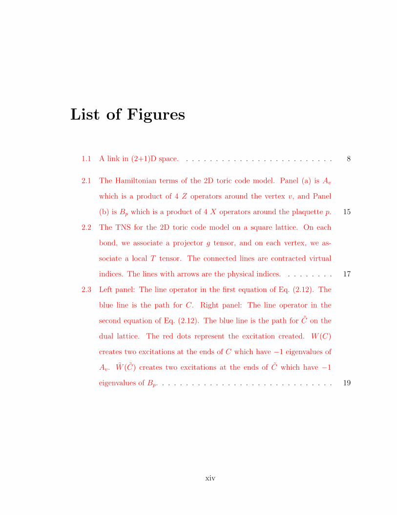
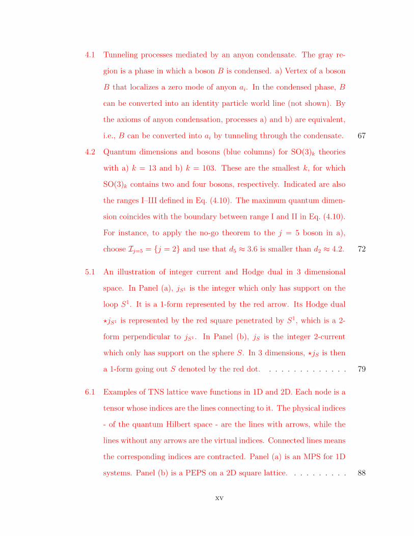


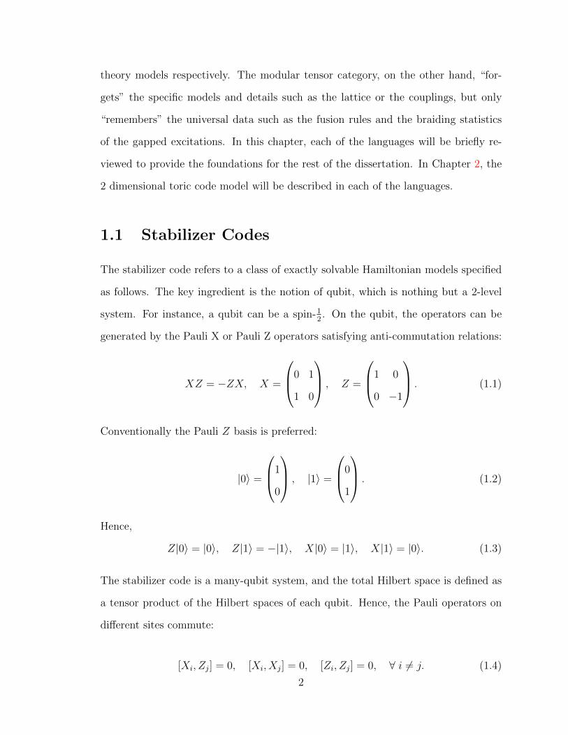
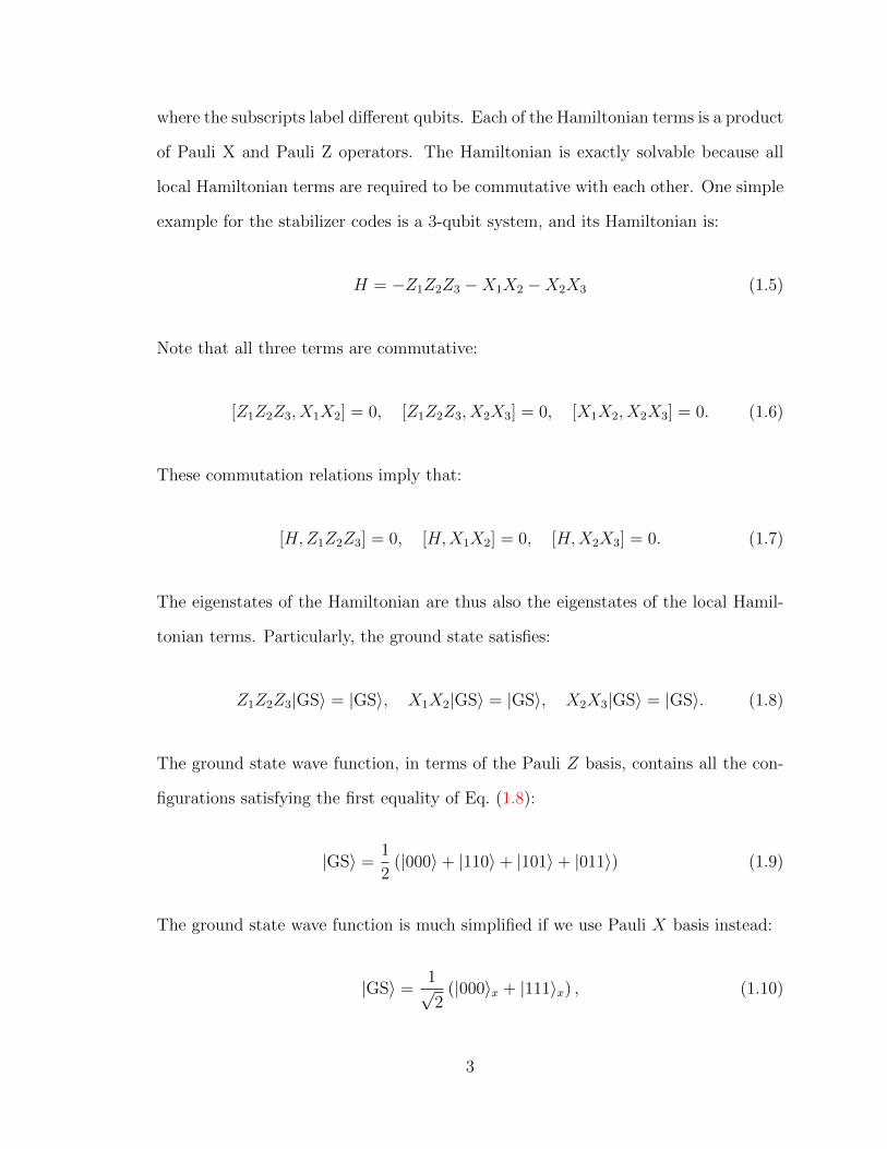
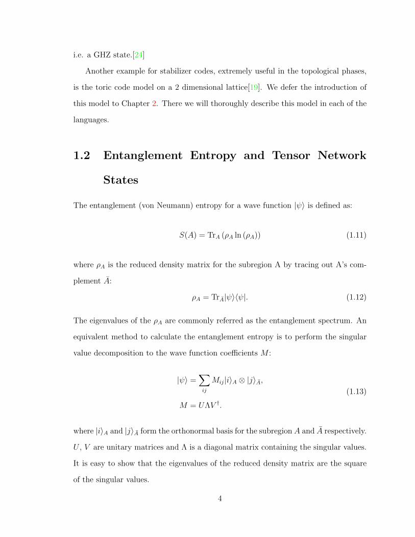

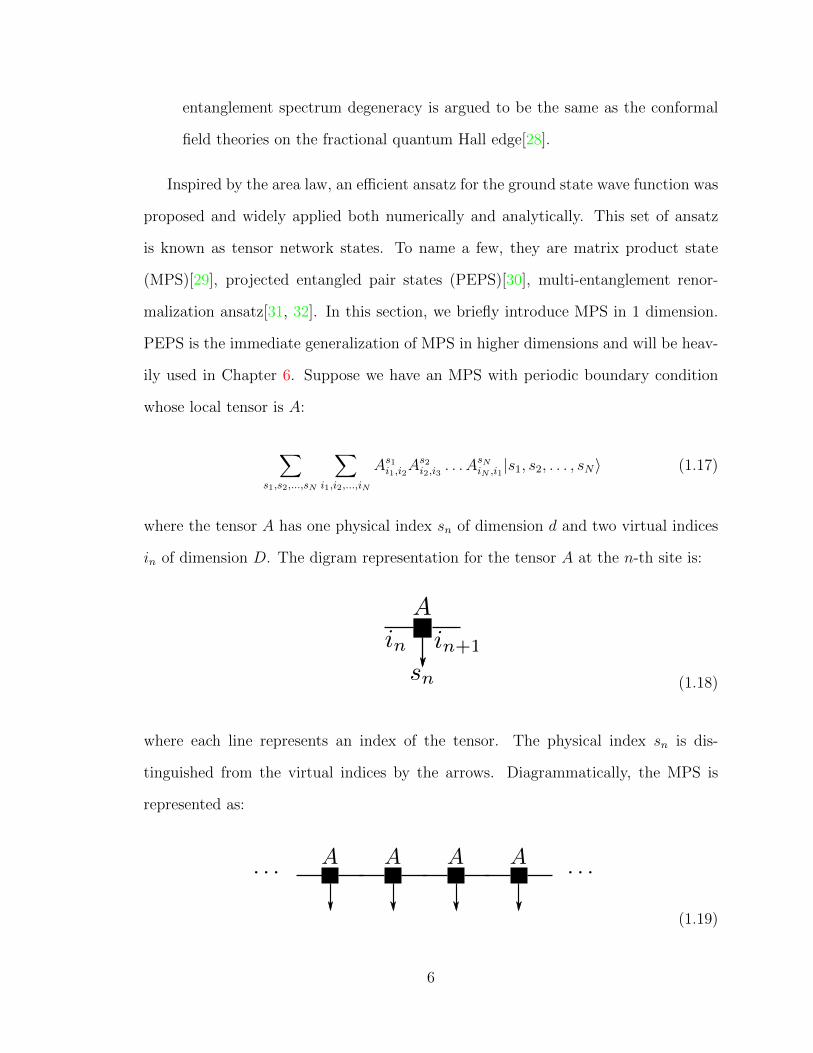


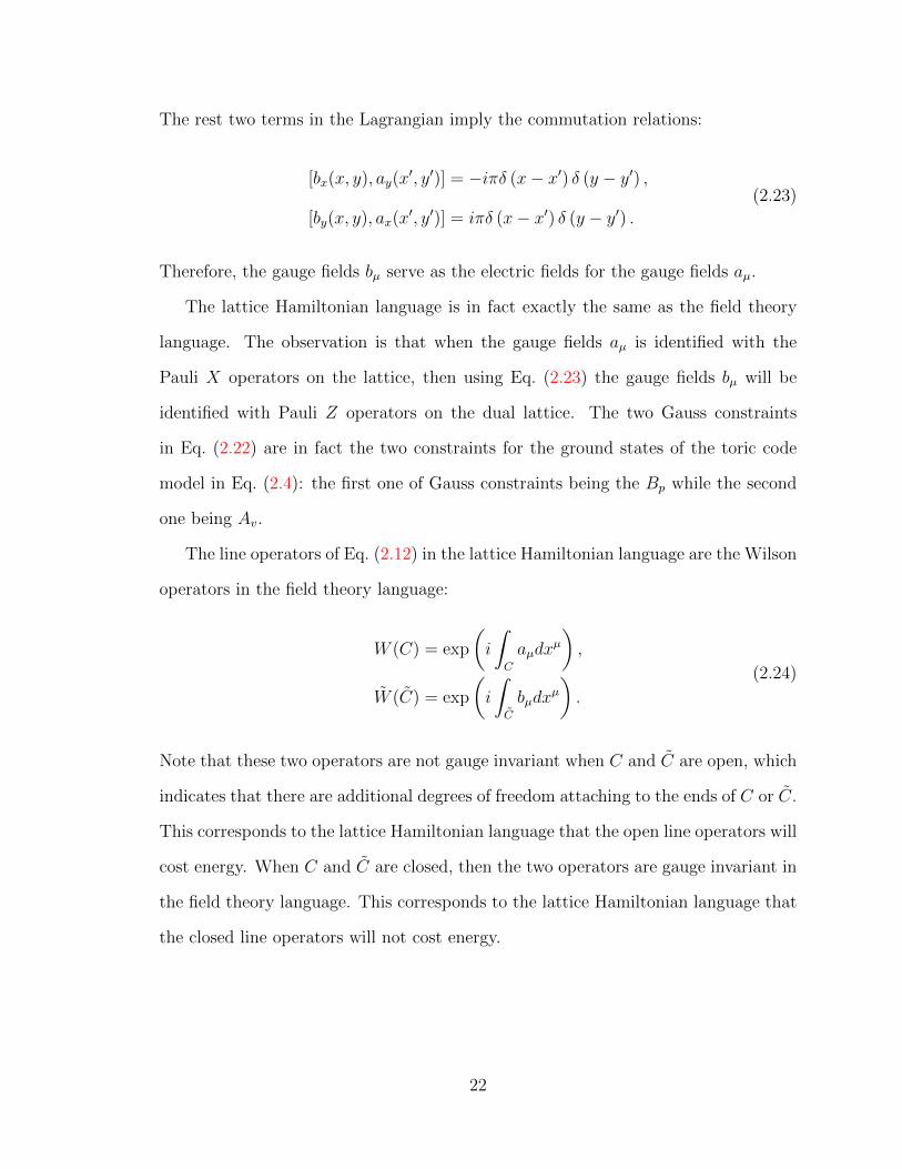


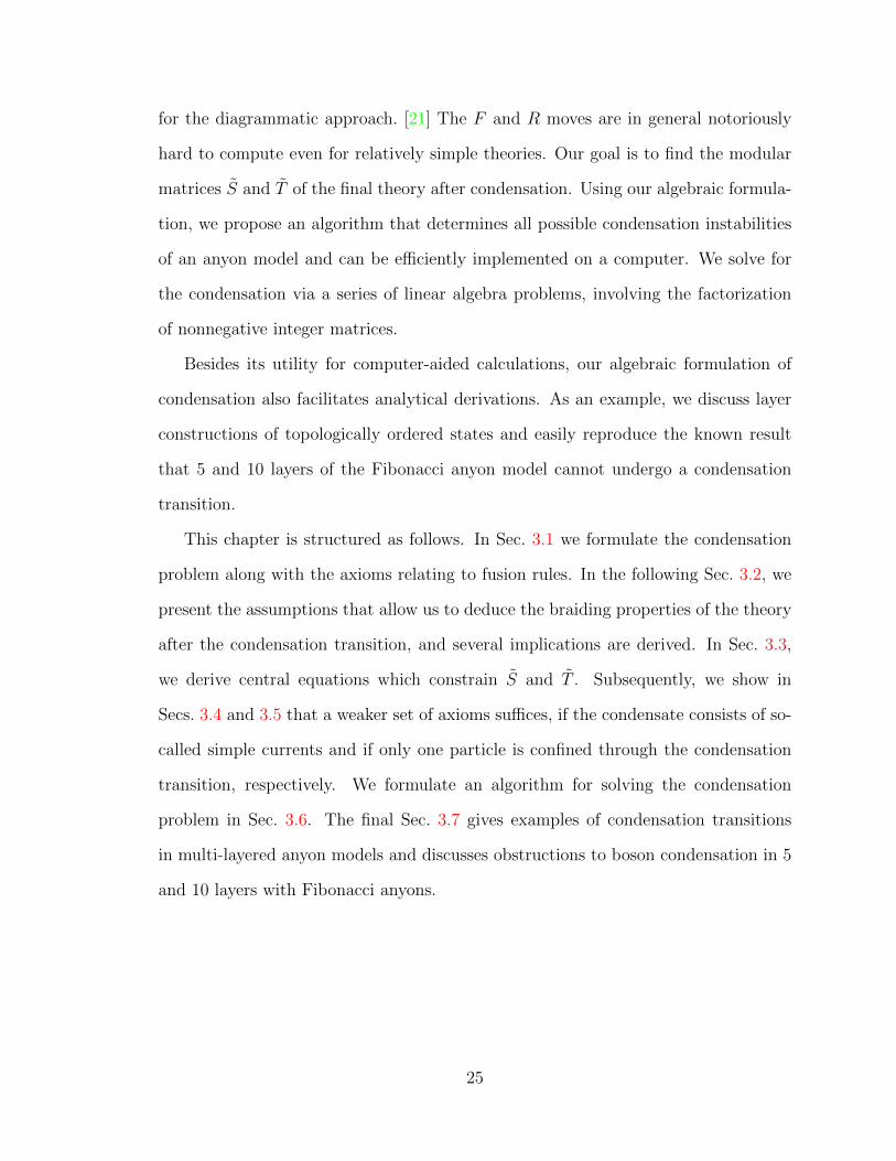

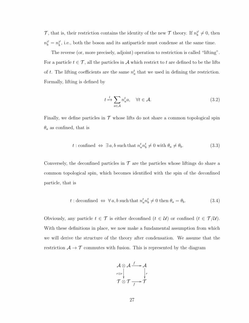
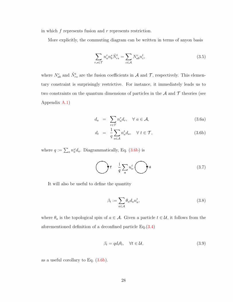


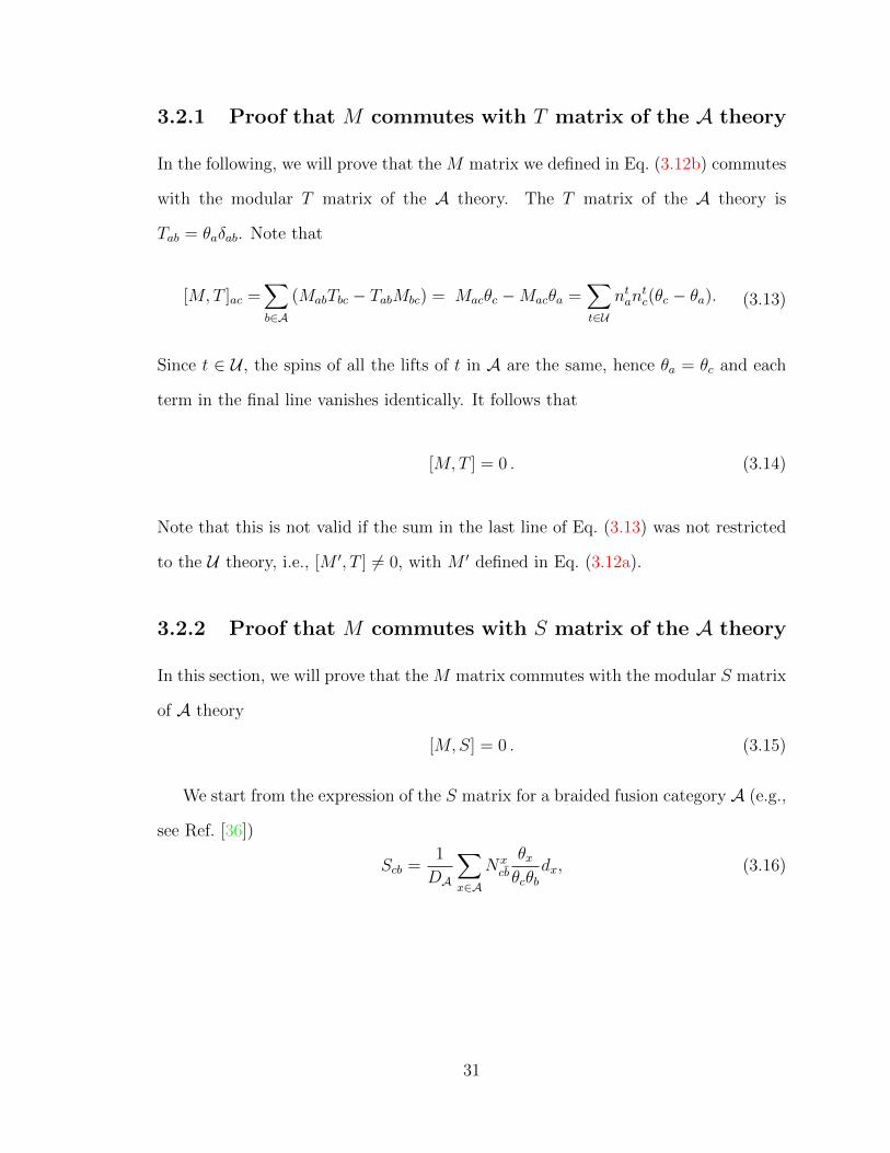

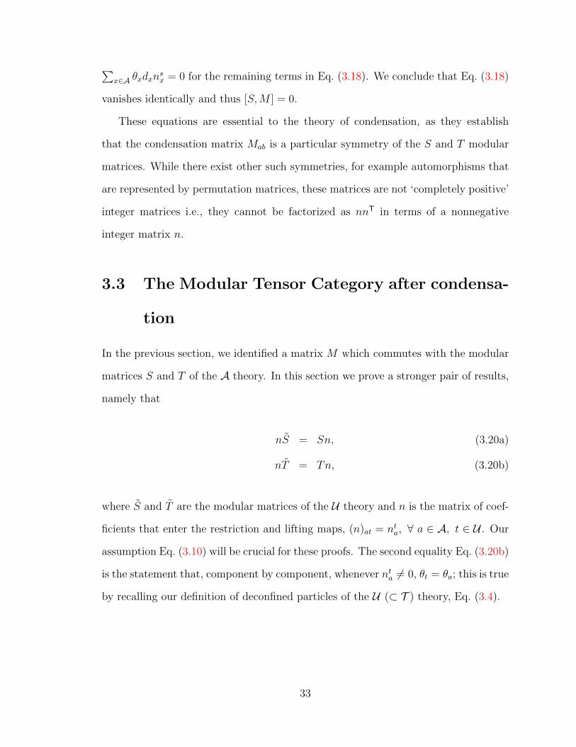

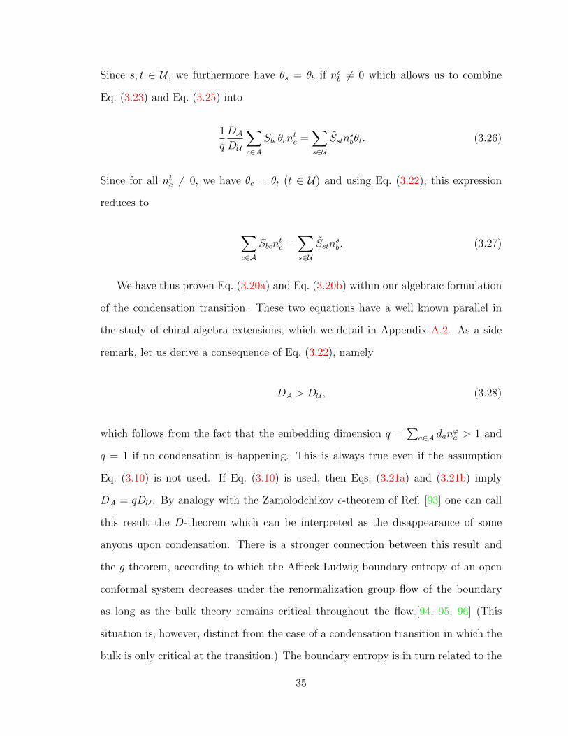


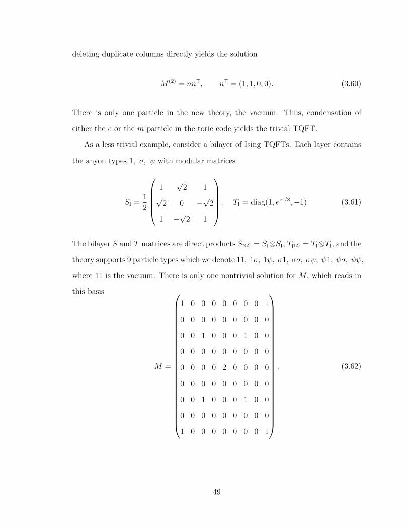


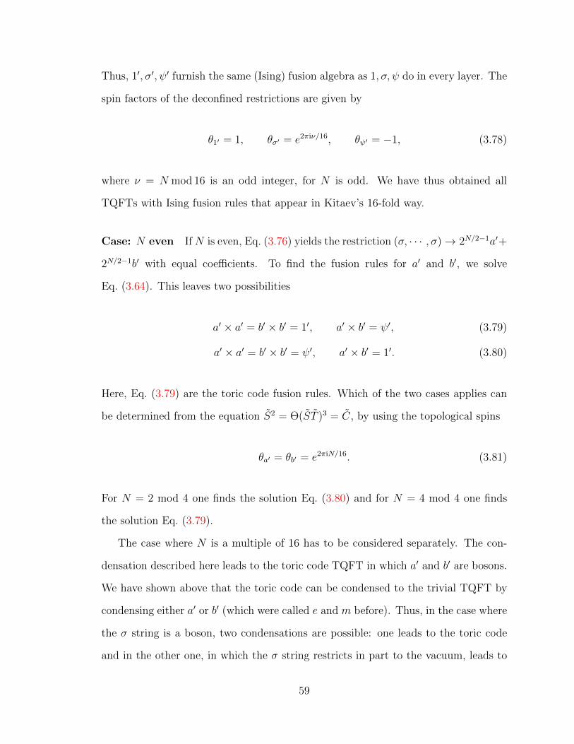


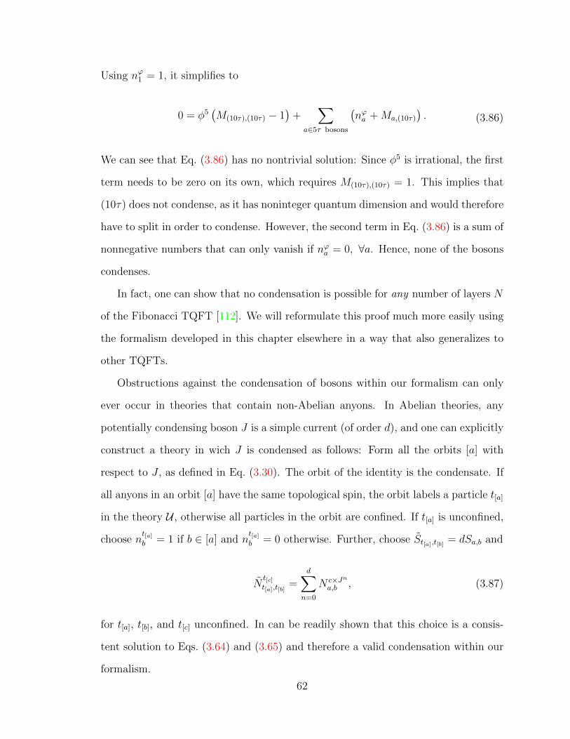


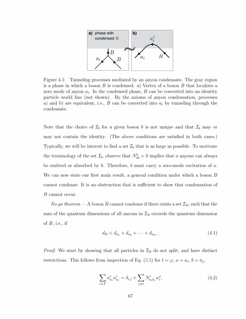

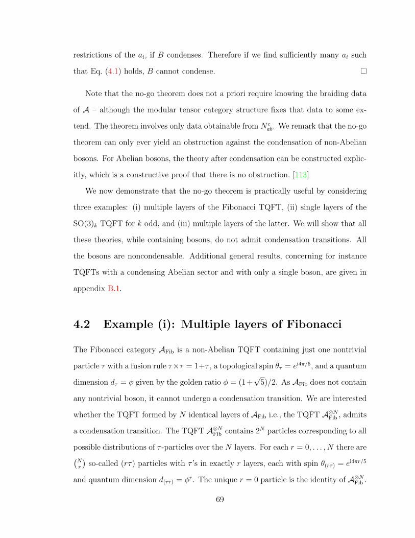
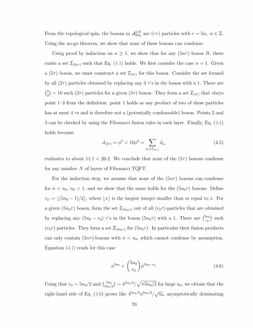

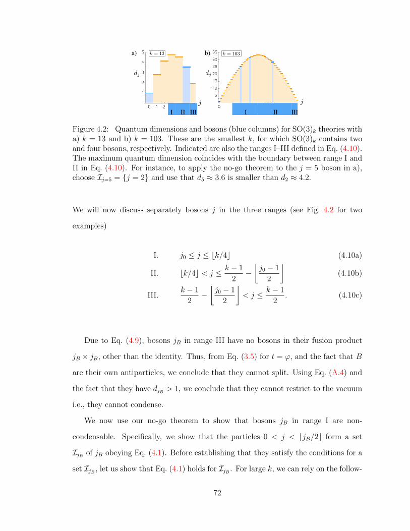


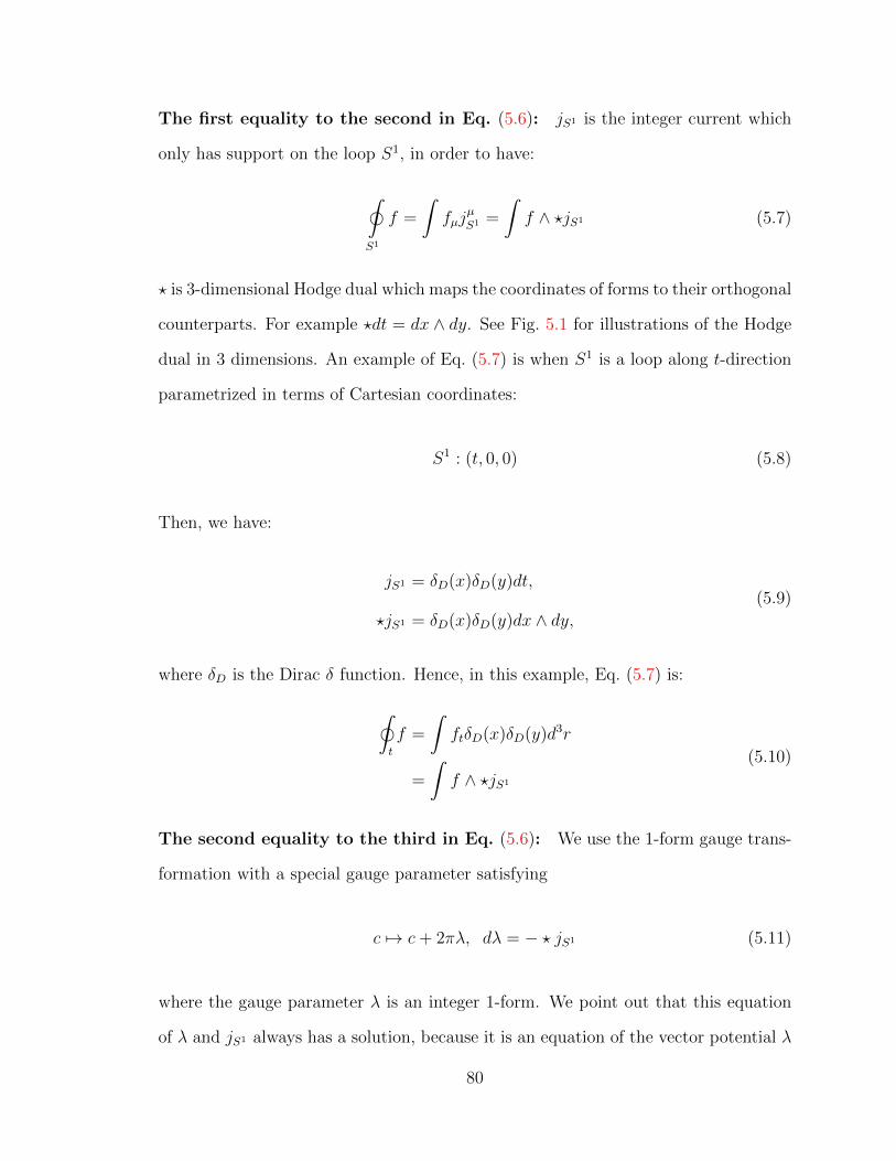


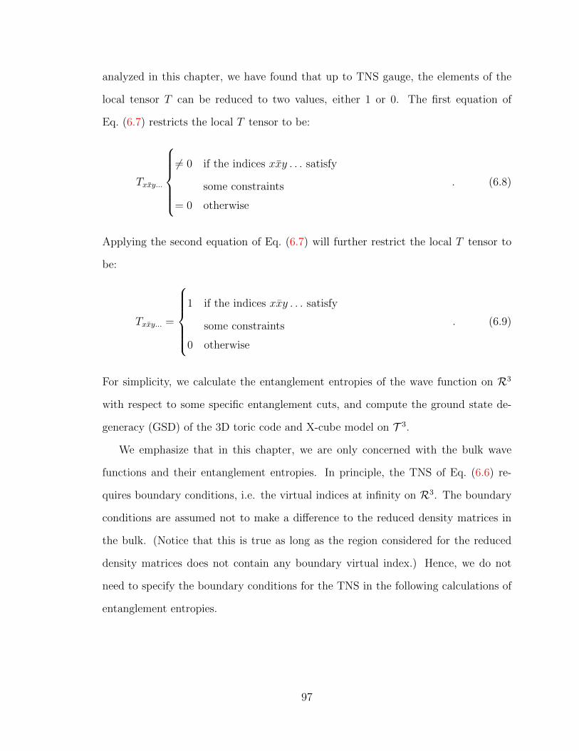
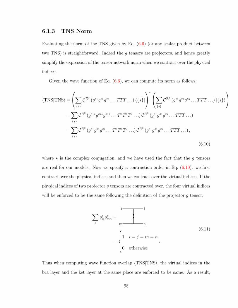


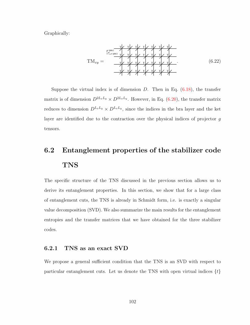
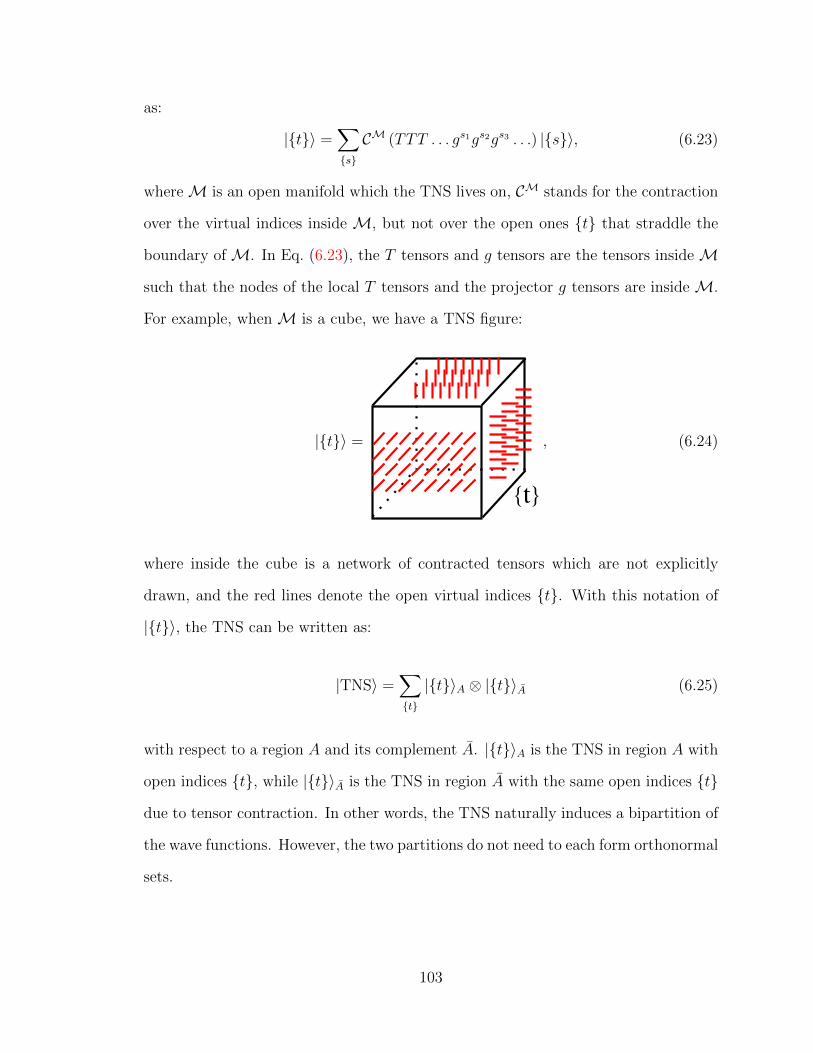

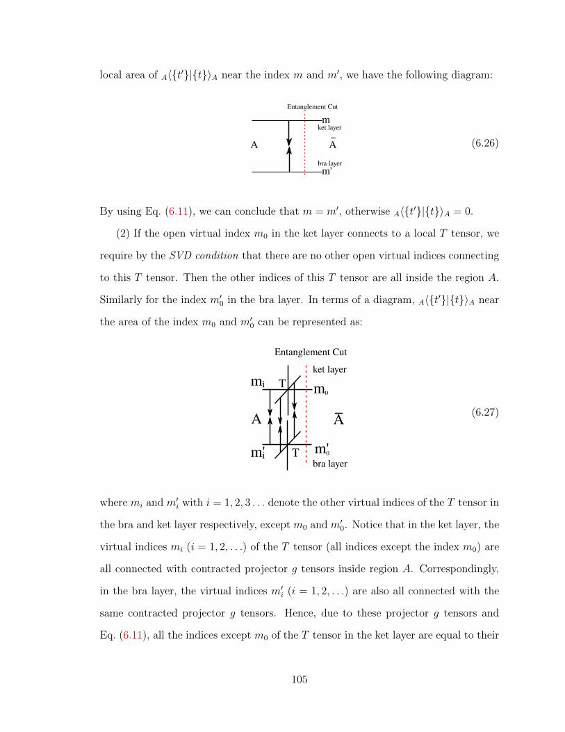


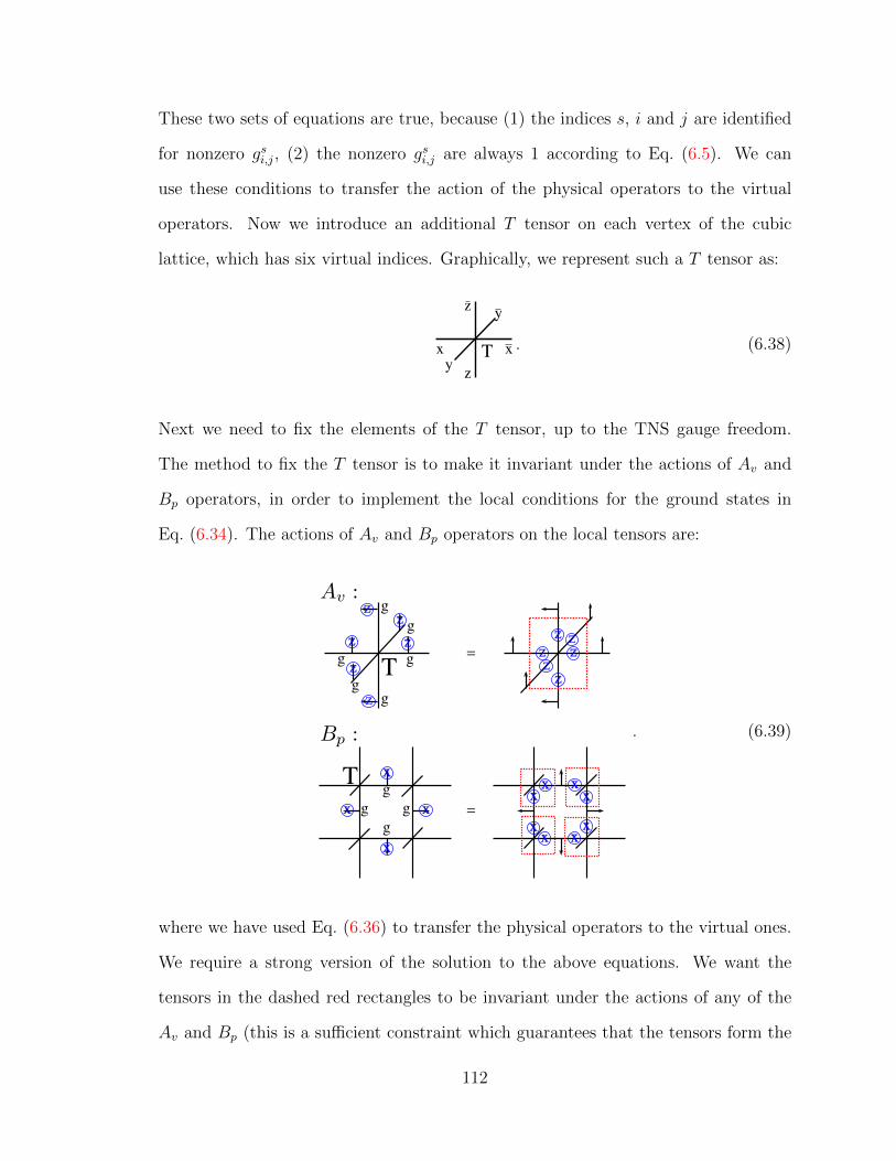


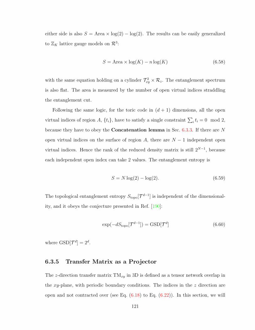


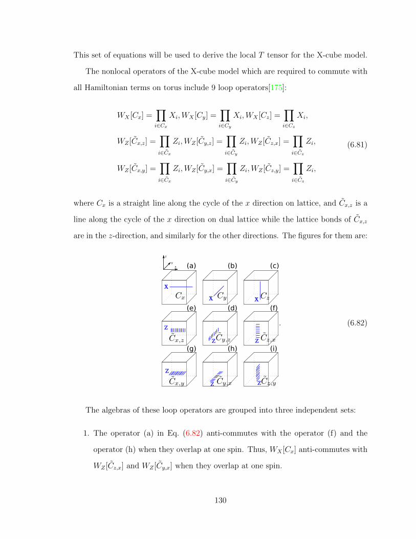

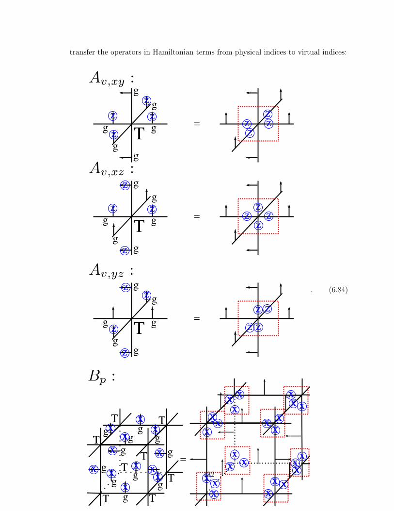


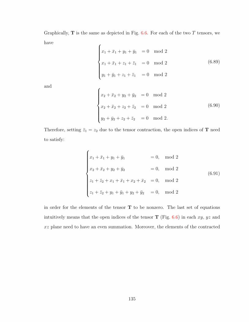


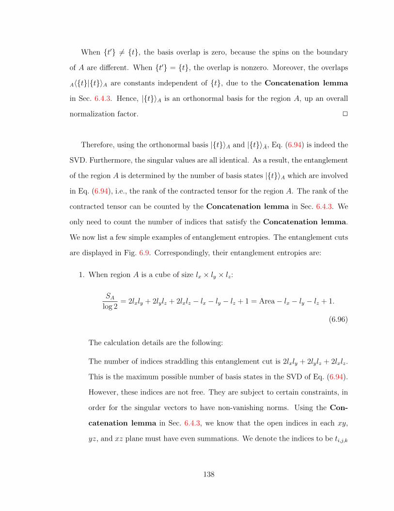

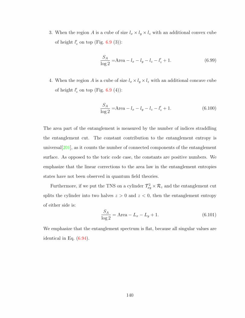
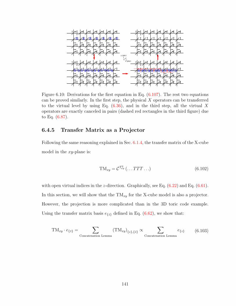
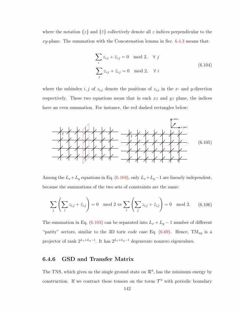


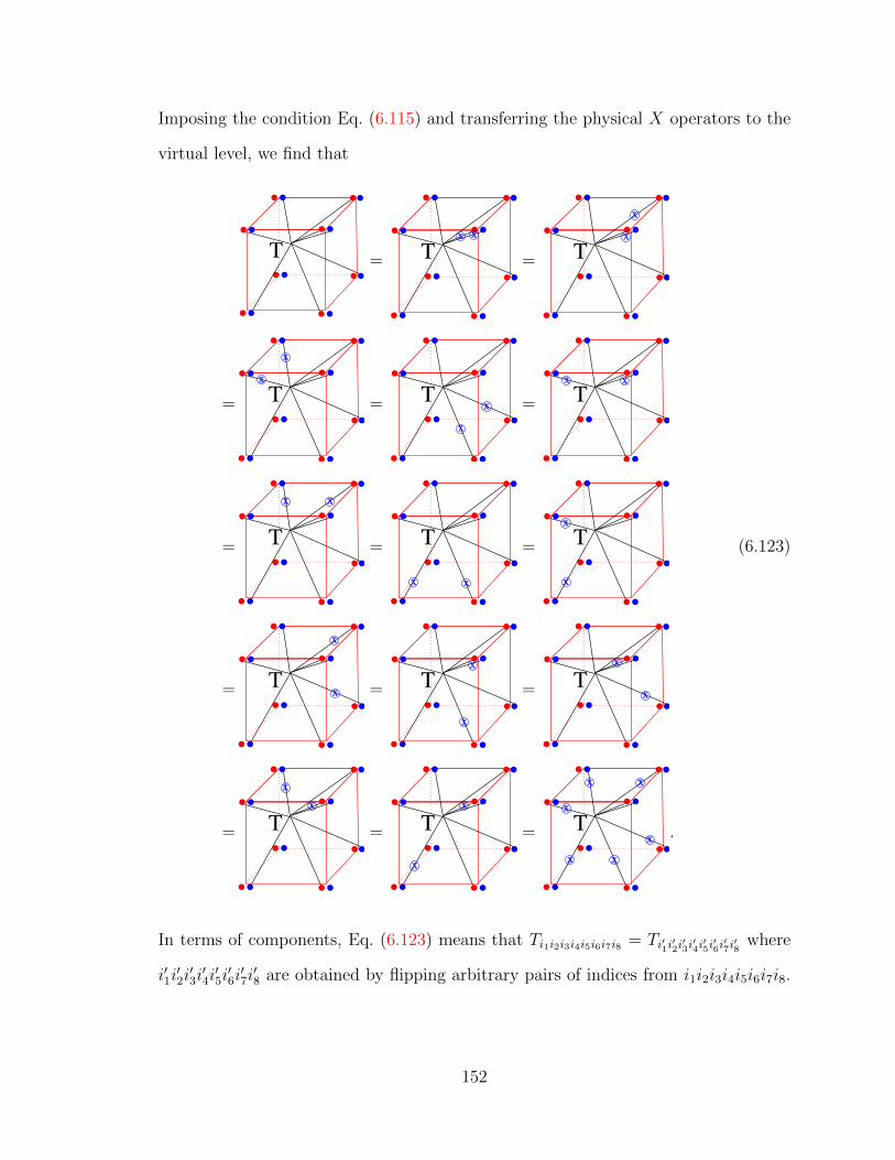


![arXiv:1108.4038v1 [cond-mat.str-el] 19 Aug 2011 · arXiv:1108.4038v1 [cond-mat.str-el] 19 Aug 2011 Entanglement Entropyof Gapped Phases and Topological Orderin Three dimensions Tarun](https://static.documents.pub/doc/80x56/5fc04e81e6a6694a225215c3/arxiv11084038v1-cond-matstr-el-19-aug-2011-arxiv11084038v1-cond-matstr-el.jpg)


![Topological Scars - pks.mpg.de · Scar characteristics Non-integrable model [Turner et. al, Nature Physics (2018)] Low (sub-volume law) entanglement entropy states No disorder (distinct](https://static.documents.pub/doc/80x56/5e067ba8a705735abc119809/topological-scars-pksmpgde-scar-characteristics-non-integrable-model-turner.jpg)


