Topology and combinatorics of Hilbert schemesof points on orbifolds

Paul Johnson

Colorado State Universitywww.math.colostate.edu/~johnson

November 4, 2013

Basics on Hilbn(C2)

Basics of the Hilbert scheme of points on a surface

Let R = C[x , y ]. Then:

Hilbn(C2) := {ideals I ⊂ R| dim R/I = n}

I Hilbn(C2) is smooth and connected

I Generically I will be the ideal sheaf of n distinct points in C2,so dim Hilbn(C2) = 2n

I When two or more points collide they become a “fat point”that remembers how they collided

For a general surface S , replace ideals with ideal sheaves

Question: What are the betti numbers of Hilbn(S)?

Warm-up: Euler-characteristic of Hilbn(C2)

Before we find the Betti numbers let’s find χ(Hilbn(C2)):

I The action of (C∗)2 on C2 induces a (C∗)2 action onHilbn(C2)

I The fixed points of the (C∗)2 action are the monomial ideals

I Since χ(C∗) = χ((C∗)2) = 0, the non-fixed orbits contributenothing to the euler characteristic

So χ(Hilbn(C2)) is the number of monomial ideals of length n.

How many monomial ideals of length n are there?

Bijection between monomial ideals and partitions

Monomials not in I are the cells of the partition. Exterior cornersof the partition are the generators of the monomial ideal.

x0y0

x0y1

x0y2

x0y3

x1y0

x1y1

x1y2

x1y3

x2y0

x2y1

x2y2

x2y3

x3y0

x3y1

x3y2

x3y3

x4y0

x4y1

x4y2

x4y3

I λ(x3, xy , y2) (2, 1, 1)

So χ(Hilbn(C2)) = p(n).

Betti numbers of Hilbn(C2)

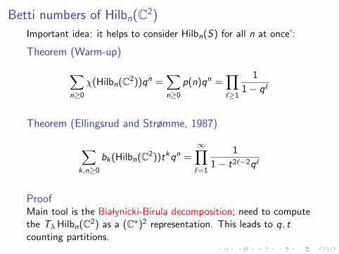
Important idea: it helps to consider Hilbn(S) for all n at once’:

Theorem (Warm-up)

∑n≥0

χ(Hilbn(C2))qn =∑n≥0

p(n)qn =∏`≥1

1

1− q`

Theorem (Ellingsrud and Strømme, 1987)

∑k,n≥0

bk(Hilbn(C2))tkqn =∞∏`=1

1

1− t2`−2q`

ProofMain tool is the Bia lynicki-Birula decomposition; need to computethe Tλ Hilbn(C2) as a (C∗)2 representation. This leads to q, tcounting partitions.

Motivation: Gottsche’s formula

Three Theorems

Theorem 1: Product Formula

Let S be a smooth quasi-projective surface with Betti numbers bi .Let S [n] = Hilbn(S)

Theorem (Gottsche, 1990)

∑k,n

bk(S [n])tkqn =∏`≥1

(1 + t2`−1q`)b1(1 + t2`+1q`)b3

(1− t2`−2q`)b0(1− t2`q`)b2(1− t2`+2q`)b4

Proof.Reduce to case S = C2 using Weil conjectures

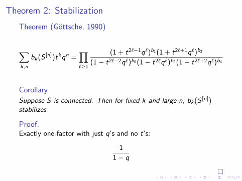
Theorem 2: Stabilization

Theorem (Gottsche, 1990)

∑k,n

bk(S [n])tkqn =∏`≥1

(1 + t2`−1q`)b1(1 + t2`+1q`)b3

(1− t2`−2q`)b0(1− t2`q`)b2(1− t2`+2q`)b4

Corollary

Suppose S is connected. Then for fixed k and large n, bk(S [n])stabilizes

Proof.Exactly one factor with just q’s and no t’s:

1

1− q

Theorem 3: Geometric Representation Theory

Theorem (Gottsche, 1990)

∑k,n

bk(S [n])tkqn =∏`≥1

(1 + t2`−1q`)b1(1 + t2`+1q`)b3

(1− t2`−2q`)b0(1− t2`q`)b2(1− t2`+2q`)b4

Theorem (Nakajima, Grojnowski)⊕Hk(Hilbn(S)) is a highest weight representation for a

Heisenberg algebra modeled on H∗(S).

Nakajima and Grojnowski reproves, and categorifies, Gottsche’sresult.

What happens when S is anorbifold?

Start with S = [C2/G ]

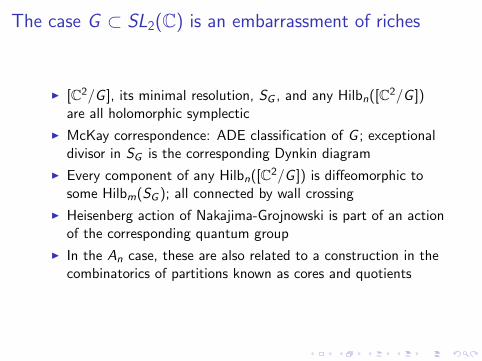
The case G ⊂ SL2(C) is an embarrassment of riches

I [C2/G ], its minimal resolution, SG , and any Hilbn([C2/G ])are all holomorphic symplectic

I McKay correspondence: ADE classification of G ; exceptionaldivisor in SG is the corresponding Dynkin diagram

I Every component of any Hilbn([C2/G ]) is diffeomorphic tosome Hilbm(SG ); all connected by wall crossing

I Heisenberg action of Nakajima-Grojnowski is part of an actionof the corresponding quantum group

I In the An case, these are also related to a construction in thecombinatorics of partitions known as cores and quotients

When G * SL2(C), much less is known

When G is abelian, localization still works, and a modification ofEllingsrud-Strømme computes bk([C2/G ]) as a (q, t) count ofpartitions. A few lines in Sage give a vast amount of data toanalyze.

Guesein-Zade, Luengo, Melle-Hernandez

For G = Z3,Z4 conjectured a product formula, but didn’t addressgeneral G .

What I’ve doneWhen G is cyclic, I have conjectural formulations of Theorems 1-3.I have a proof Theorem 2: Stabilization, using a generalization ofcores and quotients that appears to be new.

Back to Earth:

Understanding Hilbn([C2/G ])

Orbifold Hilbert Schemes are fixed point sets

Hilbn([C2/G ]) := {G -equivariant ideals I ⊂ R}= Hilbn(C2)G ⊂ Hilbn(C2)

I Hilbn([C2/G ]) is smooth: it’s a fixed point set in somethingsmooth

I Hilbn([C2/G ] is not connected. One discrete invariant: R/Iisn’t just a vector space, it’s a representation of G

I This is the only discrete invariant

For κ ∈ K0(G ), let HilbκG denote the component where R/I = κ.Then HilbκG is connected.

Colo(u)red boxes

Restrict to G = Z/rZ, with action (exp(2πi/r), exp(2πim/r)). Fora monomial ideal, keeping track of K0(G ) class is counting coloredboxes:

(1/5,1/5) (1/5,2/5) (1/5,-1/5)

Example: Hilbn([C2/Z3])

Let Z3 act on C2 diagonally: g · (x , y) = (ωx , ωy).

I Hilb1([C2/Z3]) = {(0, 0)}I Hilb2([C2/Z3]) = P1

Let v be a tangent direction at the origin:

Iv = {f ∈ R|f (0) = ∂v f (0) = 0}

I Hilb3([C2/Z3]) has two components. One component is justan isolated point m2

0 = (x2, xy , y2)

What’s R/m20 as a Z3 representation?

Z3 acts on 1 triviallyActs as the same nontrivial representation on x and y

The other component is the minimal resolution

Let p 6= (0, 0) ∈ C2. Its orbit consists of 3 points; let I be theideal sheaf of these three points. Then R/I has the regularrepresentation of G .Over the origin, there are a P1 worth of ideals that give the regularrepresentation:

I2v = {f ∈ R|f (0) = ∂v f (0) = ∂2v f (0) = 0}

This component is O(−3)→ P1, the minimal resolution of C2/Z3.

HilbGG (often called G Hilb) always gives the minimal resolution

Special McKay Correspondence

When S is smooth, Hilb1(S) = S , but Hilb1([C2/G ]) = point.The ideal sheaf of a smooth point on [C2/G ] corresponds to theregular representation of G .

TheoremHilbG

G is the minimal resolution of C2/G .

I The minimal resolution of C2/G is a tree of c rational curves

I When G ⊂ SL2, c = |G | − 1, and so χ(HilbGG ) = |G |

I Otherwise, c < |G | − 1, and HilbGG only sees a subset of theirreducible representations of G

Generating series for orbifold Hilbert schemes

Restrict to G = Z/rZ, with action (exp(2πi/r), exp(2πim/r)).

Disconnected generating series

DHm/r :=∑n,k≥0

bk(Hilbn([C2/G ]))tkqn

Call an element δ ∈ K0(G ) small if HilbδG is nonempty butcompact; equivalently, if HilbδG is nonempty but Hilbδ−GG is empty.

Connected generating series

For δ ∈ K0(G ) small, define

CHδm/r :=∑n,k≥0

bk(Hilbδ+nGG )tkqn

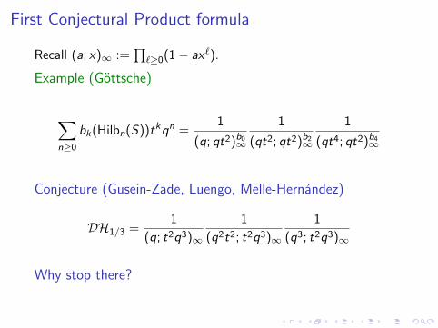
First Conjectural Product formula

Recall (a; x)∞ :=∏`≥0(1− ax`).

Example (Gottsche)

∑n≥0

bk(Hilbn(S))tkqn =1

(q; qt2)b0∞

1

(qt2; qt2)b2∞

1

(qt4; qt2)b4∞

Conjecture (Gusein-Zade, Luengo, Melle-Hernandez)

DH1/3 =1

(q; t2q3)∞

1

(q2t2; t2q3)∞

1

(q3; t2q3)∞

Why stop there?

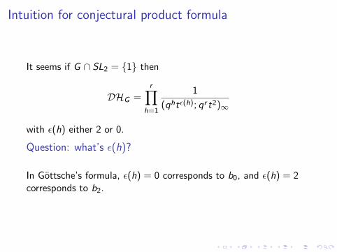
Intuition for conjectural product formula

It seems if G ∩ SL2 = {1} then

DHG =r∏

h=1

1

(qhtε(h); qr t2)∞

with ε(h) either 2 or 0.

Question: what’s ε(h)?

In Gottsche’s formula, ε(h) = 0 corresponds to b0, and ε(h) = 2corresponds to b2.

Chen-Ruan cohomology

The Chen-Ruan cohomology of [C2/G ] is rationally graded, with dwith 0 ≤ d < 4.

Idea: Round down the degree in Chen-Ruan cohomology toeither 0 or 2

Chen-Ruan cohomology of [C2/G ]

For G abelian:

I Basis given by the elements of G

I If g acts as (exp(2πia/r), exp(2πib/r)), the age of g isι(g) = a/r + b/r

I The degree of g is twice the age.

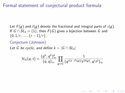
Formal statement of conjectural product formula

Let F (g) and I (g) denote the fractional and integral parts of ι(g).If G ∩ SL2 = {1}, then F (G ) gives a bijection between G and{0, 1/r , . . . , (r − 1)/r}.

Conjecture (Johnson)

Let G be cyclic, and define k = |G ∩ SL2|

HG (q, t) =(qk ; qk)k∞

(q, q)∞

∏g∈G

1

(qr(1−F (g))t2I (g), qr t2)∞

Analog of Theorem 2: Stabilization

The analogs of stabilization and geometric representation theorywork on the level of connected Hilbert scheme.

Theorem (Johnson)

Pt(Hilbδ+nGG ) stabilizes to 1/(t, t)

|G |∞

Note that the right hand side is independent of m and δ.

Proof.Combinatorics – a generalization of cores and quotients ofpartitions

Conjecture (Johnson)

The stable cohomology of Hilbδ+nG is freely generated by theChern classes of the |G | tautological bundles.

Analog of Theorem 3: Geometric Representation theory

Conjecture (Johnson)

Let δ ∈ K0(G ) be small, and G cyclic. Then⊕k≥0

H∗(Hilbδ+kGG )

admits the action of a Heisenberg algebra based on thecohomology of the minimal resolution of C2/G .

Evidence:Let c be the number of rational curves in the minimal resolution ofC2/G . Then

CHδG · (q, qt2)∞ · (qt2, qt2)c∞

has positive coefficients; but higher powers start giving negativecoefficients.

Thank you

How to calculate bk(HilbvG )

using partitions

Bia lynicki-Birula decomposition ≈ Morse theory

Suppose X has a C∗ action so that

1. limλ→0 λx exists for all x ∈ X

2. There are isolated fixed points

Then we can compute the homology of X by “Morse theory”

1. x 7→ λx is the Morse flow

2. Fixed points are critical points

What’s the Morse index of a fixed point p?

Morse index = 2 dimT−p X

At each fixed point p, TpX is a C∗ representation, and so splitsinto eigenspaces where λv = λav

a = 0 Can’t occur since fixed points are isolated

a > 0 Flowing toward p

a < 0 Flowing away from p

T−p X is the subspace where a < 0.

TheoremBia lynicki-Birula

Pt(X ) =∑

p fixed

t index(p)

Proof.The differential is zero since all fixed points have even index.

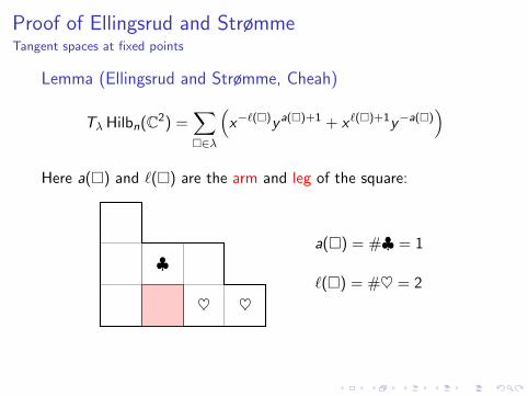
Proof of Ellingsrud and StrømmeTangent spaces at fixed points

Lemma (Ellingsrud and Strømme, Cheah)

Tλ Hilbn(C2) =∑�∈λ

(x−`(�)ya(�)+1 + x`(�)+1y−a(�)

)Here a(�) and `(�) are the arm and leg of the square:

♣

♥ ♥

a(�) = #♣ = 1

`(�) = #♥ = 2

Proof of Ellingsrud and StrømmeTangent spaces at fixed points

Lemma (Ellingsrud and Strømme, Cheah)

Tλ Hilbn(C2) =∑�∈λ

(x−`(�)ya(�)+1 + x`(�)+1y−a(�)

)Here a(�) and `(�) are the arm and leg of the square:

♣

♥ ♥

a(�) = #♣ = 1

`(�) = #♥ = 2

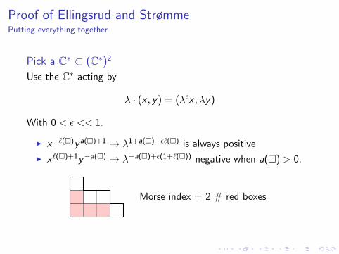
Proof of Ellingsrud and StrømmePutting everything together

Pick a C∗ ⊂ (C∗)2

Use the C∗ acting by

λ · (x , y) = (λεx , λy)

With 0 < ε << 1.

I x−`(�)ya(�)+1 7→ λ1+a(�)−ε`(�) is always positive

I x`(�)+1y−a(�) 7→ λ−a(�)+ε(1+`(�)) negative when a(�) > 0.

Morse index = 2 # red boxes

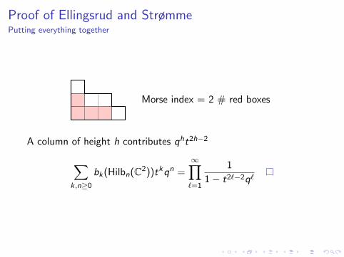
Proof of Ellingsrud and StrømmePutting everything together

Morse index = 2 # red boxes

A column of height h contributes qht2h−2

∑k,n≥0

bk(Hilbn(C2))tkqn =∞∏`=1

1

1− t2`−2q`

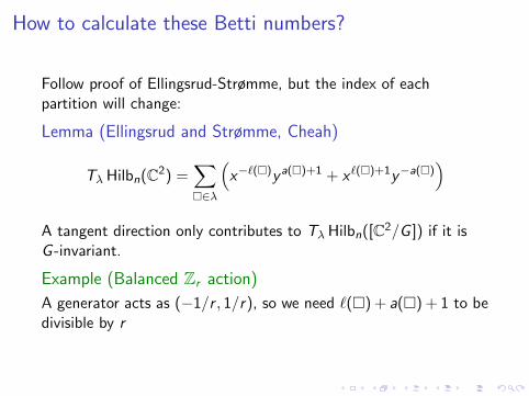
How to calculate these Betti numbers?

Follow proof of Ellingsrud-Strømme, but the index of eachpartition will change:

Lemma (Ellingsrud and Strømme, Cheah)

Tλ Hilbn(C2) =∑�∈λ

(x−`(�)ya(�)+1 + x`(�)+1y−a(�)

)A tangent direction only contributes to Tλ Hilbn([C2/G ]) if it isG -invariant.

Example (Balanced Zr action)

A generator acts as (−1/r , 1/r), so we need `(�) + a(�) + 1 to bedivisible by r