TOPOLOGY OF THE UNIVERSE: THEORY AND OBSERVATION

JEAN-PIERRE LUMINET1 AND BOUDEWIJN F. ROUKEMA2,3

1 DARC, Observatoire de Paris-Meudon, 5 place Jules Janssen,F-92195 Meudon Cedex, France (Jean-Pierre.Luminet@obspm.fr)

AND

2Institut d’Astrophysique de Paris, 98bis Bd Arago, F-75.014, Paris, France3Inter-University Centre for Astronomy and Astrophysics, Post Bag 4Ganeshkhind, Pune, 411 007, India (boud@iucaa.ernet.in)

Abstract. “One could imagine that as a result of enormously extended astronomical experience,the entire universe consists of countless identical copies of our Milky Way, that the infinite spacecan be partitioned into cubes each containing an exactly identical copy of our Milky Way. Wouldwe really cling on to the assumption of infinitely many identical repetitions of the same world?. . .We would be much happier with the view that these repetitions are illusory, that in realityspace has peculiar connection properties so that if we leave any one cube through a side, thenwe immediately reenter it through the opposite side.” (Schwarzschild 1900, translation 1998)

Developments in the theoretical and observational sides of cosmic topology were slow formost of the century, but are now progressing rapidly, at the scale of most interest which is1-10h−1 Gpc rather than 10kpc.

The historical, mathematical and observational sides of this subject are briefly reviewed inthis course.

1. Introduction

Think of a right triangle drawn on a transparency. The transparency is a piece of an infiniteEuclidean plane whose flat metric is expressed by Pythagoras’ Theorem. Bend the transparencyaround into a cylinder. The latter is thus obtained by identifying two opposite edges of thetransparency. The new surface is locally flat (Pythagoras’ Theorem stills holds perfectly), but ithas a quite different shape. It contains closed geodesics. Next we can identify the two remainingedges and get a flat torus (this is a thought experiment, because the usual torus, or “annulus”,visualized as a surface of revolution in 3–dimensional Euclidean space, has positive Gaussiancurvature at some places and negative at others). The flat torus has still a locally Euclideanmetric although its global shape has drastically changed: it is a finite surface without borders.

These elementary operations well illustrate the difference between the curvature (given bythe metric) and the topology. Both are needed in order to know the full geometry of a two-dimensional, or more importantly, a three-dimensional space. This applies as well to physicalspace, namely to cosmological models for describing the Universe as a whole. The shape ofspace is a fundamental issue in physics. Curiously enough, this Cargese ’98 summer school oncosmology is probably the first one to include a couple of lectures on cosmic topology. As we

2

shall see below, both for historical and for practical reasons, cosmic topology has been widelyignored during 80 years of relativistic cosmology, except by some pioneering authors.

After an historical section 2, sections 3-4 are mostly based on the review paper by [45] (here-after LaLu 95). Since the mid 90’s, worldwide interest for cosmological topology has blossomed,from a mathematical point of view, mostly related to progress in the understanding of compacthyperbolic manifolds, from a theoretical point of view, as well as from an observational point ofview, related to improvements of data on the large scale 3–dimensional distribution of cosmicobjects and on the 2–dimensional structure of the cosmic microwave background. Since theselectures are aimed to provide a general view of the subject, only some of the new mathematicalresults (obtained since the 1995 revival) will be mentioned. An incomplete list of theoreticalarticles related to the possible physical origin of cosmic topology is provided towards the end ofsection 2. For the latest developments in all aspects of the subject, see the proceedings of the1997 and 1998 workshops [76, 67]. Section 5 of this lecture, devoted to the observational aspectsof cosmic topology, provides an up-date and complement to the review of [69].

2. A Brief History of Cosmological Topology

Most of this historical introduction is taken from [55], see also [75].Is space finite or infinite, oriented or not, made of one piece or not, has it holes or handles,

what is its global shape? A common misconception is to believe that Einstein’s general relativitytheory is all one needs to answer such paramount questions. However, general relativity dealsonly with local geometrical properties of the universe, such as its curvature, not with its globalcharacteristics, namely its topology.

The physical extension of space is one of the oldest cosmological questions, going back totwenty–five centuries of cosmological modelling (e.g. [56]). In the history of cosmology, it is wellknown that Newtonian physical space, mathematically identified with the infinite Euclideanspace R3, gave rise to paradoxes such as the darkness of the night sky (see e.g. [38]) and toproblems of boundary conditions.

Wondering about absolute accelerations, Newton imagined a bucket swung on the end of arope and compared it with a bucket at rest. If the bucket is at rest, the surface of the waterremains flat. If the bucket rotates, the water surface becomes concave. Newton argued that theconcave shape of the water could not be due to its relative motion with respect to the bucket,and that it proved the existence of an absolute centrifugal acceleration. Mach considered thesame problem and criticised Newton’s reasoning [2]: what we observe is that the bucket rotateswith respect to the fixed stars, but, who is to say whether the bucket is really rotating withrespect to the stars at rest or whether the stars are really rotating with respect to the bucket?According to Newton, we should observe the concavity in the first case and not in the second.This is because Newton assumed an absolute frame related to the global distribution of matterin the universe (the fixed stars). Mach denied the concept of absolute acceleration. Accordingto him, a rotating body in a non-rotating universe or a non-rotating body in a rotating universeshould give the same result: centrifugal force. Mach concluded that the inertial mass of a bodyshould result from the contributions of all the masses in the universe. But an obvious divergencedifficulty arose, since a homogeneous Newtonian universe with non–zero density has an infinitemass. Hence, Mach supported the idea of a finite universe in order to have a finite local inertia.

By the end of the XIXth century, mathematicians such as Riemann had discovered a va-riety of finite spaces without boundaries, such as the hypersphere and the projective space.Schwarzschild [72] brought this work to the attention of the astronomical community in 1900,and he considered the possibility that the space could have a non–trivial topology: “One couldimagine that as a result of enormously extended astronomical experience, the entire universeconsists of countless identical copies of our Milky Way, that the infinite space can be partitioned

3

into cubes each containing an exactly identical copy of our Milky Way. Would we really clingon to the assumption of infinitely many identical repetitions of the same world? . . .We wouldbe much happier with the view that these repetitions are illusory, that in reality space has pecu-liar connection properties so that if we leave any one cube through a side, then we immediatelyreenter it through the opposite side” (English translation [73]).

In modern terms, Schwarzschild told us that if the galaxies were found to lie in a rectangularlattice, with images of the same galaxy repeating at equivalent lattice points, then we couldconclude that the Universe is a 3–torus.

Cosmology developed rapidly after Einstein’s 1915 discovery of general relativity. Generalrelativity explains gravity as the curvature of spacetime; the latter is determined by the densityof matter–energy. The aim of relativistic cosmology is to deduce from the gravitational fieldequations some physical models of the Universe as a whole. When Einstein (1917) assumedin his static cosmological solution that space was a positively–curved hypersphere, one of hisstrongest motivations was to provide a model for a finite space, although without a boundary.Following Mach and Riemann, he regarded the closure of space as necessary to solve the problemof inertia and chose the hypersphere as his model of space.

The Einstein space model cleared up most of the paradoxes stemming from Newtonian cos-mology in such an elegant way that most cosmologists of the time adopted the new paradigm ofa closed space, without examining other geometrical possibilities. Einstein was also convincedthat the hypershere provided not only the metric of cosmic space – namely its local geometri-cal properties – but also its global structure, its topology. However, topology does not seem tohave been a major preoccupation of Einstein; his 1917 cosmological article did not mention anytopological alternative to the spherical space model.

Some of his colleagues pointed out to Einstein the arbitrariness of his choice. Indeed theglobal shape of space is not only depending on the metric; it depends primarily on its topology,and requires a complemenraty approach to Riemannian differential geometry. Since Einstein’sequations are partial derivative equations, they describe only local geometrical properties ofspacetime. The latter are contained in the metric tensor, which enables us to calculate thecomponents of the curvature tensor at any non-singular point of spacetime. But Einstein’sequations do not fix the global structure of spacetime: to a given metric solution of the fieldequations, correspond several (and in most cases an infinite number of) topologically distinctuniverse models.

Firstly, de Sitter [14] noticed that the Einstein’s solution admitted a different spaceform,the 3-dimensional projective space (also called elliptic space), obtained from the hypersphere byidentifying antipodal points. The projective space has the same metric as the spherical one, buta different topology (for instance, for the same curvature radius its volume is half that of thespherical space).

H. Weyl also pointed out the freedom of choice between spherical and elliptical topologies.Einstein’s answer [18] was unequivocal: “Nevertheless I have like an obscure feeling which leadsme to prefer the spherical model. I have a feeling that manifolds in which any closed curve can becontinuously contracted to a point are the simplest ones. Other persons must share this feeling,otherwise astronomers would have taken into account the case where our space is Euclidean andfinite. Then the two-dimensional Euclidean space would have the connectivity properties of aring surface. It is an Euclidean plane in which any phenomenon is doubly periodic, where pointslocated in the same periodical grid are identical. In finite Euclidean space, three classes of noncontinuously contractible loops would exist. In a similar way, the elliptical space possesses a classof non continuously contractible loops, contrary to the spherical case; it is the reason why I like itless than the spherical space. Can it be proved that elliptical space is the only variant of sphericalspace? It seems yes to me”.

4

Einstein [19] repeated his argumentation in a postcard sent to Felix Klein: “I would like togive you a reason why the spherical case should be preferred to the elliptical case. In sphericalspace, any closed curve can be continuously contracted to a point, but not in the elliptical space;in other words the spherical space alone is simply-connected, not the elliptical one [...] Finitespaces of arbitrary volume with the Euclidean metric element undoubtedly exist, which can beobtained from infinite spaces by assuming a triple periodicity, namely identity between sets ofpoints. However such possibilities, which are not taken into account by general relativity, havethe wrong property to be multiply-connected”.

From these remarks it seems that the Einstein’s preference for simple–connectedness of spacewas of an aesthetical nature, rather than being based on physical reasoning.

In his answer to Weyl, Einstein was definitely wrong on the last point: in dimension three,an infinite number of topological variants of the spherical space – all closed – do exist, includ-ing the so-called lens spaces (whereas in dimension two, only two spherical spaceforms exist, theordinary sphere and the elliptic plane). However, nobody knew this result in the 1920’s: the topo-logical classification of 3–dimensional spaces was still at its beginnings. The study of Euclideanspaceforms started in the context of crystallography. Feodoroff [30] classified the 18 symmetrygroups of crystalline structures in R3, Bieberbach [4] developed a full theory of crystallographicgroups, and it took twenty years before Novacki [59] showed how Bieberbach’s results could beapplied to complete the classification of 3–dimensional Euclidean spaceforms. The case of spher-ical spaceforms was first treated by Klein [43] and Killing [44]. The problem was fully solvedmuch later [87]. Eventually, the classification of homogeneous hyperbolic spaces shot forward inthe 1970’s; it is now an open field of intensive mathematical research [79, 80].

Returning to relativistic cosmology, the discovery of non-static solutions by Friedmann [32]and, independently, Lemaıtre [48], opened a new era for models of the universe as a whole(see, e.g., [54] for an epistemological analysis). Although Friedmann and Lemaıtre are generallyconsidered as the discoverers of the big bang concept — at least of the notion of a dynamicaluniverse evolving from an initial singularity — one of their most original considerations, devotedto the topology of space, was overlooked. As they stated, the homogeneous isotropic universemodels (F–L models) admit spherical, Euclidean or hyperbolic spacelike sections according to thesign of their (constant) curvature (respectively positive, zero or negative). In addition, Friedmann[33] pointed out the topological indeterminacy of the solutions in his popular book on generalrelativity, and he emphasized how Einstein’s theory was unable to deal with the global structureof spacetime. He gave the simple example of the cylinder. Generalizing the argument to higherdimensions, he concluded that several topological spaces could be used to describe the samesolution of Einstein’s equations.

Topological considerations were fully developed in his second cosmological article, althoughprimarily devoted to the analysis of hyperbolic solutions. Friedmann [34] clearly outlined thefundamental limitations of relativistic cosmology:“Without additional assumptions, Einstein’sworld equations do not answer the question of the finiteness of our universe”, he wrote. Thenhe described how space could be finite (and multi-connected) by suitably identifying points.He also predicted the possible existence of “ghost” images of astronomical sources, since at thesame point of a multi–connected space an object and its ghosts would coexist. He added that “aspace with positive curvature is always finite”, but he recognized the fact that the mathematicalknowledge of his time did not allow him to “solve the question of finiteness for a negatively–curved space”.

By contrast with Einstein’s reasoning, it is seen that the Russian cosmologist had no prejudicein favour of a simply-connected topology. Certainly, Friedmann believed that only finite volumespaces were physically realistic. Prior to his discovery of hyperbolic solutions, the cosmologicalsolutions derived by Einstein, de Sitter and himself had a positive spatial curvature, thus a finitevolume. With negatively–curved spaces, the situation became problematic, because the “natural”

5

topology of hyperbolic space has an infinite volume. It is the reason why Friedmann, in orderto justify the physical pertinence of his solutions, emphasized the possibility of compactifyingspace by suitable identifications of points.

Lemaıtre fully shared the common belief in the closure of space. He expressed his view thatRiemannian geometry “dissipated the nightmare of infinite space” [51]. Thus Lemaıtre [48, 49]assumed positive space curvature, but he thoroughly discussed the possibility of projective space,that he preferred to the spherical one. Later, he [50] also noticed the possibility of hyperbolicand Euclidean spaces with finite volumes for describing the physical universe.

Such fruitful ideas of cosmic topology remained widely ignored by the main stream of bigbang cosmology. Perhaps the Einstein–de Sitter [20] model, which assumed Euclidean spaceand eluded the topological question, had a negative influence on the development of the field.Almost all subsequent textbooks and monographs on relativistic cosmology assumed that theglobal structure of the universe was either the finite hypersphere, or the infinite Euclideanspace, or the infinite hyperbolic space, without mentioning at all the topological indeterminacy.As a consequence, some confusion settled down about the real meaning of the terms “open”and “closed” used to characterize the F–L solutions. Whereas they apply correctly to timeevolution (open models stand for ever–expanding universes, closed models stand for expanding–contracting solutions), they do not properly describe the extension of space (open for infinite,closed for finite). Nevertheless it is still frequent to read that the (closed) spherical model hasa finite volume whereas the (open) Euclidean and hyperbolic models have infinite volumes. Thecorrespondance is true only in the very special case of a simply–connected topology and a zerocosmological constant. According to Friedmann’s original remark, in order to know if a space isfinite or infinite, it is not sufficient to determine the sign of its spatial curvature, or equivalentlyin a cosmological context to measure the ratio Ω0 of the average density to the critical value:additional assumptions are necessary — those arising from topology, precisely.

The idea of a multi–connected universe has never been entirely forgotten. In a very com-prehensive article, Ellis [21] detailed the classification of 3–dimensional Riemannian manifoldsuseful for cosmology and started to explore the observational consequences of a toroidal uni-verse. Others, such as Sokoloff and Schvartsman, Fang and Sato, Gott, Fagundes, investigatedflat and non-flat spaces (see complete references in LaLu95). Nevertheless, until 1995, investi-gations in cosmic topology were rather scarce. From an epistemological point of view, it seemsthat the prejudice in favour of simply–connected (rather than multi–connected) spaces was ofthe same kind as the prejudice in favour of static (rather than dynamical) cosmologies dur-ing the 1920’s. At a first glance, “Occam’s razor” (often useful in physical modelling) couldbe invoked to preferably select the simply–connected topologies. However, on the theoreticalside, new approaches to spacetime, such as quantum cosmology, suggest that the smallest closedhyperbolic manifolds are favoured, thus providing a new paradigm for what is the “simplest”manifold. On the observational side, present astronomical data (e.g. [12]) indicate that the av-erage density of the observable universe is less than the critical value (Ω0 = 0.3 − 0.4), thussuggesting that we live in a negatively–curved F–L universe (unless the cosmological constantis positive and large enough). Putting together theory and observation, cosmologists must facethe fact that a negatively–curved space can have a finite volume, and that in that case it mustbe multi–connected.

In the last few decades, much effort in observational and theoretical cosmology has beendirected towards determining the curvature of the universe. The problem of the topology ofspacetime was generally ignored within the framework of classical relativistic cosmology. Itbegan to be taken seriously discussed in quantum gravity for various reasons: the spontaneousbirth of the Universe from a quantum vacuum requires the Universe to have compact spacelikehypersurfaces, and the closure of space is a necessary condition to render tractable the integralsof quantum gravity [1].

6

Further work in quantum gravity and particle physics which explores ideas of space-timetopology globally and/or as the basis of a quantum gravity theory includes that of [39, 88, 57,7, 41, 16, 15, 64, 17, 74].

However, the topology of spacetime also enters in a fundamental way in classical generalrelativity. Many cosmologists were surprisingly unaware of how topology and cosmology could fittogether to provide new insights in universe models. Aimed to create a new interest in the field ofcosmic topology, the review by LaLu95 stressed what multi–connectedness of the Universe wouldmean and on its observational consequences. However two different papers ([78] ; [13]) declaredthat the small universe idea was “no longer an interesting cosmological model”. However, theauthors drew very general conclusions from considering only a few special 3-manifolds in theEuclidean case, and by adopting assumptions on the primordial perturbation spectrum whichare observationally justified on large scales only by assuming simple connectedness. They didnot take into account a very interesting class of realistic universe models, namely the compacthyperbolic manifolds, which require a quite different treatment. Ironically, approximately thesame amount of papers in cosmic topology have been published within the last 3 years as in theprevious 80 years !

3. Mathematical background

3.1. BASICS OF TOPOLOGY

The topological properties of a manifold are those which remain insensitive to continuous trans-formations. Thus, size and distance are in some sense ignored in topology: stretching, squeezingor “kneading” a manifold change the metric but not the topology; cutting, tearing or makingholes and handles change the latter. It is often possible to visualize two–dimensional manifolds byrepresenting them as embedded in three–dimensional Euclidean space (such a mapping does notnecessarily exist however, e.g. the Klein bottle and the flat torus). Three–dimensional manifoldsrequire the introduction of more abstract representations, using, for example, the fundamentaldomain.

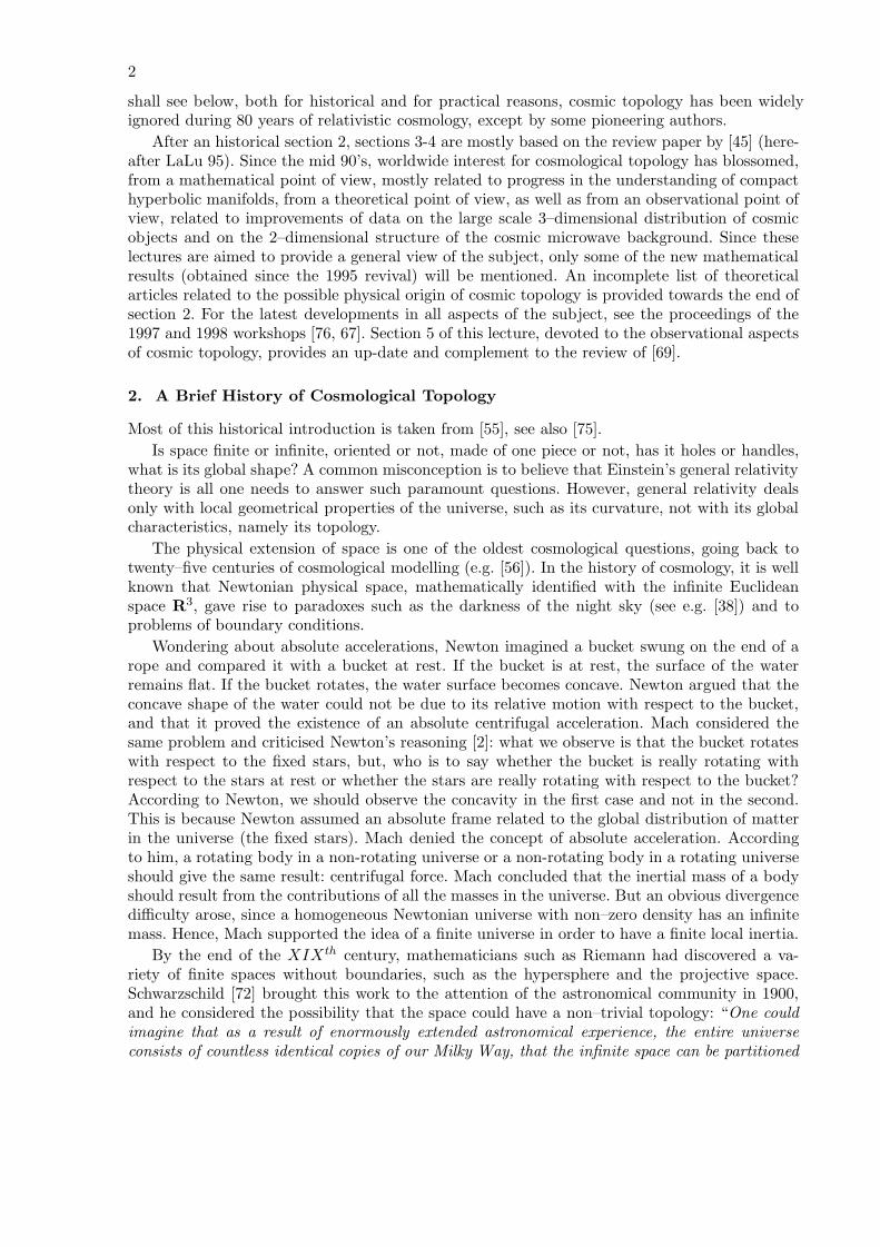
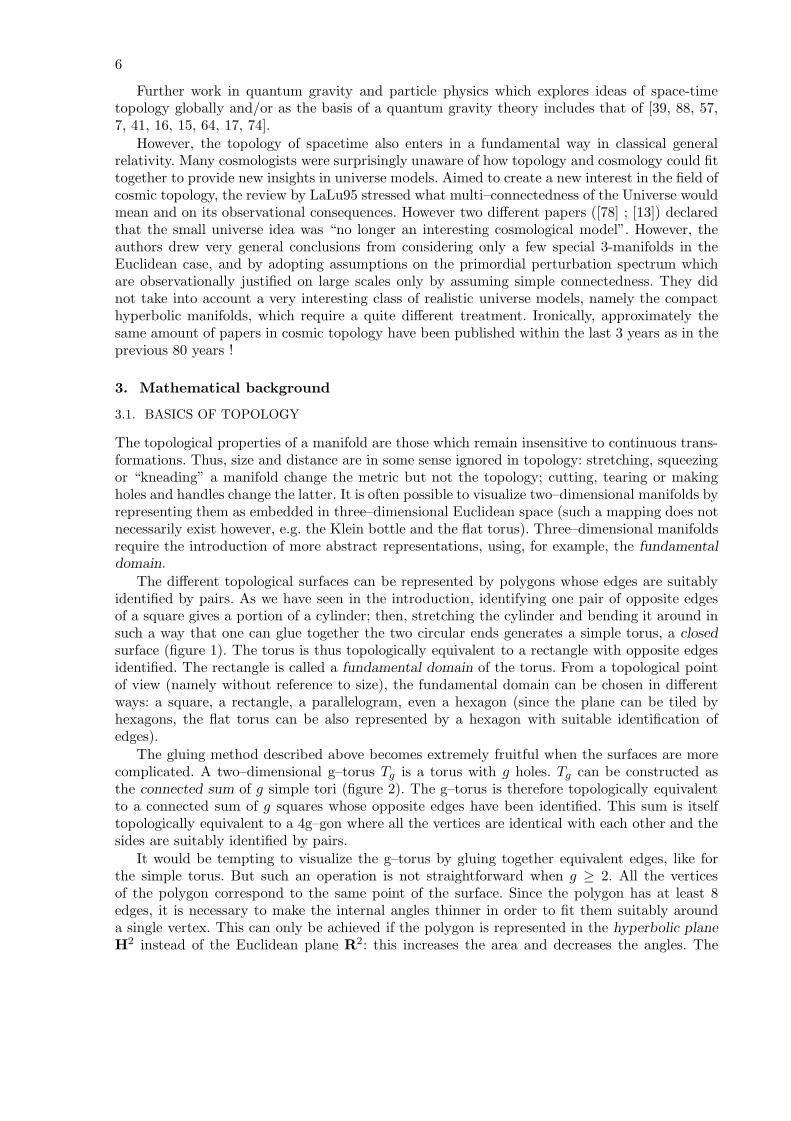
The different topological surfaces can be represented by polygons whose edges are suitablyidentified by pairs. As we have seen in the introduction, identifying one pair of opposite edgesof a square gives a portion of a cylinder; then, stretching the cylinder and bending it around insuch a way that one can glue together the two circular ends generates a simple torus, a closedsurface (figure 1). The torus is thus topologically equivalent to a rectangle with opposite edgesidentified. The rectangle is called a fundamental domain of the torus. From a topological pointof view (namely without reference to size), the fundamental domain can be chosen in differentways: a square, a rectangle, a parallelogram, even a hexagon (since the plane can be tiled byhexagons, the flat torus can be also represented by a hexagon with suitable identification ofedges).

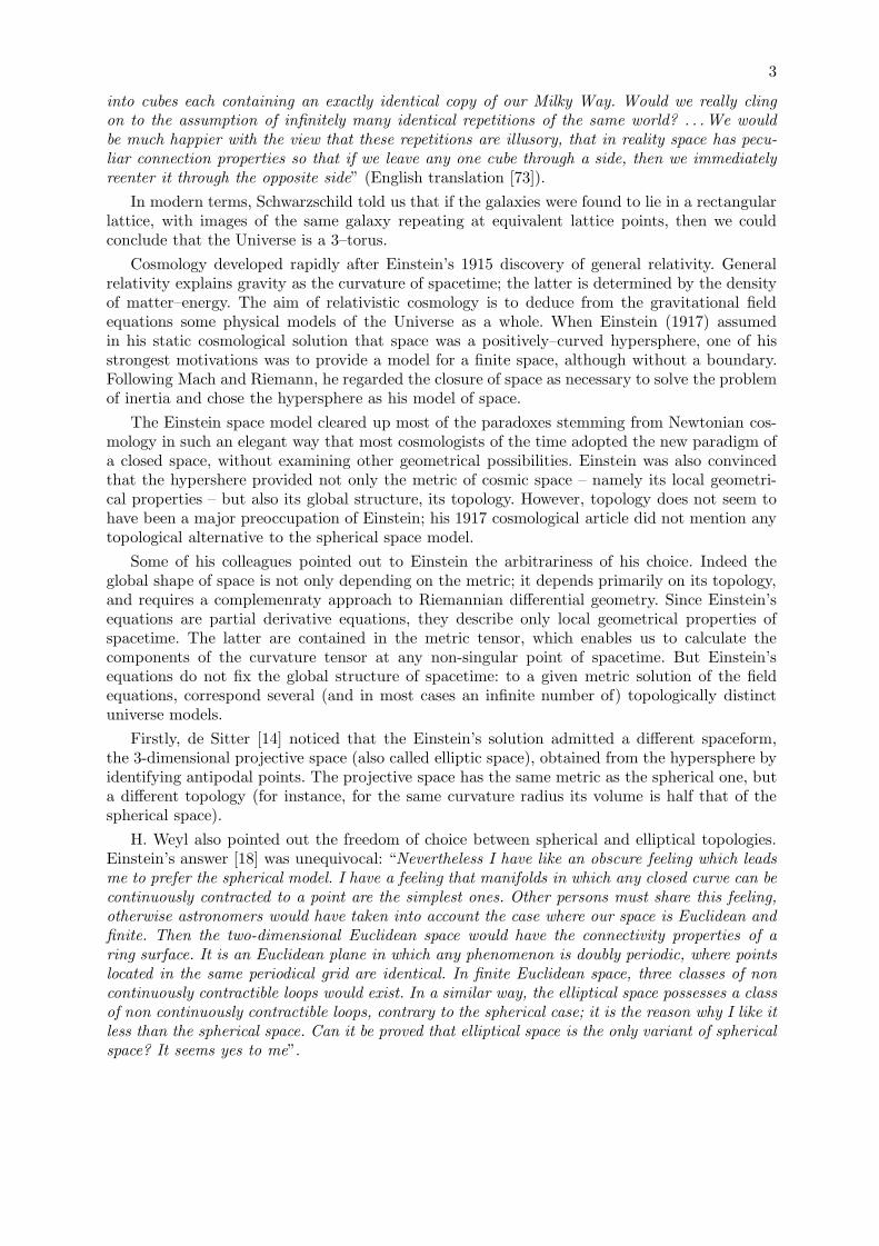
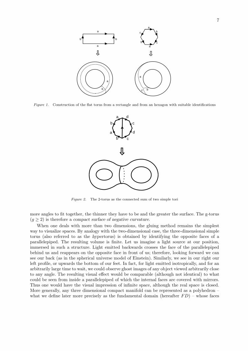
The gluing method described above becomes extremely fruitful when the surfaces are morecomplicated. A two–dimensional g–torus Tg is a torus with g holes. Tg can be constructed asthe connected sum of g simple tori (figure 2). The g–torus is therefore topologically equivalentto a connected sum of g squares whose opposite edges have been identified. This sum is itselftopologically equivalent to a 4g–gon where all the vertices are identical with each other and thesides are suitably identified by pairs.

It would be tempting to visualize the g–torus by gluing together equivalent edges, like forthe simple torus. But such an operation is not straightforward when g ≥ 2. All the verticesof the polygon correspond to the same point of the surface. Since the polygon has at least 8edges, it is necessary to make the internal angles thinner in order to fit them suitably arounda single vertex. This can only be achieved if the polygon is represented in the hyperbolic planeH2 instead of the Euclidean plane R2: this increases the area and decreases the angles. The

7

a

b

a

b

a

a

b

bc

c

a

b

a

bc

Figure 1. Construction of the flat torus from a rectangle and from an hexagon with suitable identifications

a

a

b

b c

d

c

d

Figure 2. The 2-torus as the connected sum of two simple tori

more angles to fit together, the thinner they have to be and the greater the surface. The g-torus(g ≥ 2) is therefore a compact surface of negative curvature.

When one deals with more than two dimensions, the gluing method remains the simplestway to visualize spaces. By analogy with the two-dimensional case, the three-dimensional simpletorus (also referred to as the hypertorus) is obtained by identifying the opposite faces of aparallelepiped. The resulting volume is finite. Let us imagine a light source at our position,immersed in such a structure. Light emitted backwards crosses the face of the parallelepipedbehind us and reappears on the opposite face in front of us; therefore, looking forward we cansee our back (as in the spherical universe model of Einstein). Similarly, we see in our right ourleft profile, or upwards the bottom of our feet. In fact, for light emitted isotropically, and for anarbitrarily large time to wait, we could observe ghost images of any object viewed arbitrarily closeto any angle. The resulting visual effect would be comparable (although not identical) to whatcould be seen from inside a parallelepiped of which the internal faces are covered with mirrors.Thus one would have the visual impression of infinite space, although the real space is closed.More generally, any three dimensional compact manifold can be represented as a polyhedron –what we define later more precisely as the fundamental domain (hereafter FD) – whose faces

8

p

γγ '

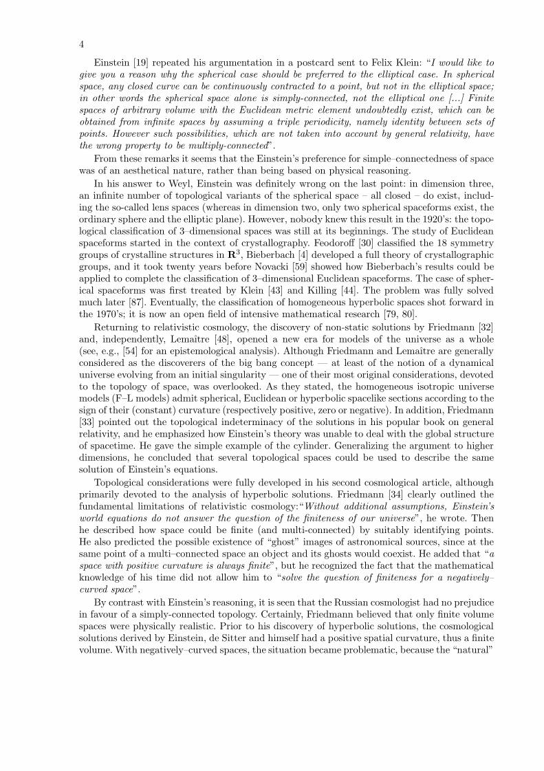
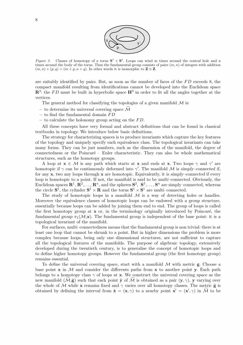
Figure 3. Classes of homotopy of a torus S1 × S1. Loops can wind m times around the central hole and ntimes around the body of the torus. Thus the fundamental group consists of pairs (m, n) of integers with addition(m, n) + (p, q) = (m + p, n + q). In other words it is isomorphic to Z⊕ Z.

are suitably identified by pairs. But, as soon as the number of faces of the FD exceeds 8, thecompact manifold resulting from identifications cannot be developed into the Euclidean spaceR3: the FD must be built in hyperbolic space H3 in order to fit all the angles together at thevertices.

The general method for classifying the topologies of a given manifold M is:− to determine its universal covering space M− to find the fundamental domain FD− to calculate the holonomy group acting on the FD.

All these concepts have very formal and abstract definitions that can be found in classicaltextbooks in topology. We introduce below basic definitions.

The strategy for characterizing spaces is to produce invariants which capture the key featuresof the topology and uniquely specify each equivalence class. The topological invariants can takemany forms. They can be just numbers, such as the dimension of the manifold, the degree ofconnectedness or the Poincare – Euler characteristic. They can also be whole mathematicalstructures, such as the homotopy groups.

A loop at x ∈ M is any path which starts at x and ends at x. Two loops γ and γ′ arehomotopic if γ can be continuously deformed into γ′. The manifold M is simply–connected if,for any x, two any loops through x are homotopic. Equivalently, it is simply–connected if everyloop is homotopic to a point. If not, the manifold is said to be multi–connected. Obviously, theEuclidean spaces R1, R2,. . . , Rn, and the spheres S2, S3,. . . , Sn are simply–connected, whereasthe circle S1, the cylinder S1 ×R and the torus S1 × S1 are multi–connected.

The study of homotopic loops in a manifold M is a way of detecting holes or handles.Moreover the equivalence classes of homotopic loops can be endowed with a group structure,essentially because loops can be added by joining them end to end. The group of loops is calledthe first homotopy group at x or, in the terminology originally introduced by Poincare, thefundamental group π1(M,x). The fundamental group is independent of the base point: it is atopological invariant of the manifold.

For surfaces, multi–connectedness means that the fundamental group is non trivial: there is atleast one loop that cannot be shrunk to a point. But in higher dimensions the problem is morecomplex because loops, being only one–dimensional structures, are not sufficient to captureall the topological features of the manifolds. The purpose of algebraic topology, extensivelydeveloped during the twentieth century, is to generalise the concept of homotopic loops andto define higher homotopy groups. However the fundamental group (the first homotopy group)remains essential.

To define the universal covering space, start with a manifold M with metric g. Choose abase point x in M and consider the differents paths from x to another point y. Each pathbelongs to a homotopy class γ of loops at x. We construct the universal covering space as thenew manifold (M,g) such that each point y of M is obtained as a pair (y, γ), y varying overthe whole of M while x remains fixed and γ varies over all homotopy classes. The metric g isobtained by defining the interval from x = (x, γ) to a nearby point x′ = (x′, γ) in M to be

9

equal to the interval from x to x′ in M. By construction, (M,g) is locally indistinguishablefrom (M,g). But its global – namely topological – properties can be quite different. It is clearthat, when M is simply–connected, it is identical to its universal covering space M. When Mis multi–connected, each point of M generates an infinite number of points in M. The universalcovering space can thus be thought of as an “unwrapping” of the original manifold.

Consider a point x and a loop γ at x in M. If γ lies entirely in a simply-connected domainof M, (x, γ) generates a single point x in M. Otherwise, it generates additional points x′, x′′,. . . which are said to be homologous to x. The displacements x 7→ x′, x 7→ x′′, . . . are isometriesand form the so-called holonomy group Γ in M. This group is discontinuous, i.e., there is anon zero shortest distance between any two homologous points, and the generators of the group(except the identity) have no fixed point. This last property is very restrictive (it excludes forinstance the rotations) and allows the classification of all possible holonomy groups.

Equipped with such properties, the holonomy group is said to act freely and discontinuouslyon M. The holonomy group is isomorphic to the fundamental group π1(M).

The geometrical properties of a manifold M within a simply–connected domain are the sameas those of its development in the universal covering M. The largest simply–connected domaincontaining a given point x of M, namely the set y ∈ M, d(y, x) ≤ d(y, γ(x)),∀γ ∈ Γ, is calledthe fundamental domain (FD).

The FD is always convex and has a finite number of faces (due to the fact that the holonomygroup is discrete). These faces are homologous by pairs ; the displacements carrying one face toanother are the generators of the holonomy group Γ.

In two dimensions, the FD is a surface whose boundary is constituted by lines, thus apolygon. In three dimensions, it is a volume bounded by faces, thus a polyhedron.

The configuration formed by the fundamental polyhedron FD and its images γFD (γ ∈ Γ)is called a tesselation of M, each image γFD being a cell of the tesselation.

The FD has two major advantages:

− The fundamental group of a given topological manifold M is isomorphic to the fundamentalgroup of the FD. Routine methods are available to determine the holonomy group of apolyhedron.

− The FD allows one to represent any curve in M, since any portion of a curve lying outsidethe FD can be carried inside it by appropriate holonomies.

3.2. TWO-DIMENSIONAL MANIFOLDS

In addition to pedagogical and illustrative interest, the classification of two–dimensional Rieman-nian surfaces plays an important role in physics for understanding (2+1)–dimensional gravity,a toy model to gain insight into the real world of (3+1)–dimensional quantum gravity.

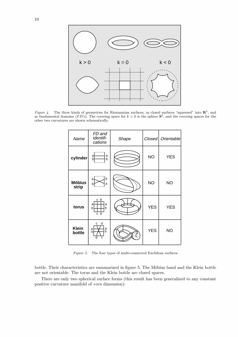
Any Riemannian surface is homeomorphic to a surface admitting a metric with constantcurvature k. Thus, any Riemannian surface can be expressed as the quotient M = M/Γ, wherethe universal covering space M is either (figure 4):

− the Euclidean plane R2 if k = 0− the sphere S2 if k > 0− the hyperbolic plane H2 if k < 0.

and Γ is a discrete subgroup of isometries of M without fixed point.To characterise the quotient spaces we adopt the following abbreviations:C = closed, O = open, SC = simply–connected, MC = multi–connected, OR = orientable,

NOR = non-orientable.Locally Euclidean surfaces fall into only 5 types: the simply–connected Euclidean plane itself

R, the multi–connected cylinder R × S1, the Mobius band, the torus S1 × S1 and the Klein

10

k > 0 k = 0 k < 0

Figure 4. The three kinds of geometries for Riemannian surfaces, as closed surfaces “squeezed” into R3, andas fundamental domains (FD’s). The covering space for k > 0 is the sphere S2, and the covering spaces for theother two curvatures are shown schematically.

NameFD andidentifi-cations

Shape Closed Orientable

ab b

b

b

b b

bb

a

aa

a a

a a

c d

d c

YES

YES

NO

NO YES

NO

YES

NO

cylinder

Möbius strip

torus

Kleinbottle

c d

c d

Figure 5. The four types of multi-connected Euclidean surfaces

bottle. Their characteristics are summarized in figure 5. The Mobius band and the Klein bottleare not orientable. The torus and the Klein bottle are closed spaces.

There are only two spherical surface forms (this result has been generalized to any constantpositive curvature manifold of even dimension):

11

J

JJ

J

J

J J

J

1

2

34

5

6

7 8

a1

a2a1

a2

a3

a4

a3a4

-1

-1

-1

-1

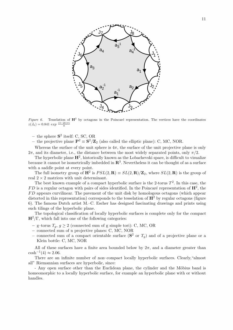
Figure 6. Tesselation of H2 by octagons in the Poincare representation. The vertices have the coordinates

z(Jk) = 0.841 exp (3−2k)πi8

− the sphere S2 itself: C, SC, OR− the projective plane P2 ≡ S2/Z2 (also called the elliptic plane): C, MC, NOR.

Whereas the surface of the unit sphere is 4π, the surface of the unit projective plane is only2π, and its diameter, i.e., the distance between the most widely separated points, only π/2.

The hyperbolic plane H2, historically known as the Lobachevski space, is difficult to visualizebecause it cannot be isometrically imbedded in R3. Nevertheless it can be thought of as a surfacewith a saddle point at every point.

The full isometry group of H2 is PSL(2,R) ≡ SL(2,R)/Z2, where SL(2,R) is the group ofreal 2× 2 matrices with unit determinant.

The best known example of a compact hyperbolic surface is the 2-torus T 2. In this case, theFD is a regular octagon with pairs of sides identified. In the Poincare representation of H2, theFD appears curvilinear. The pavement of the unit disk by homologous octagons (which appeardistorted in this representation) corresponds to the tesselation of H2 by regular octagons (figure6). The famous Dutch artist M.–C. Escher has designed fascinating drawings and prints usingsuch tilings of the hyperbolic plane.

The topological classification of locally hyperbolic surfaces is complete only for the compactH2/Γ, which fall into one of the following categories:

− g–torus Tg, g ≥ 2 (connected sum of g simple tori): C, MC, OR− connected sum of n projective planes: C, MC, NOR− connected sum of a compact orientable surface (S2 or Tg) and of a projective plane or a

Klein bottle: C, MC, NOR

All of these surfaces have a finite area bounded below by 2π, and a diameter greater thancosh−1(4) ≈ 2.06.

There are an infinite number of non–compact locally hyperbolic surfaces. Clearly,“almostall” Riemannian surfaces are hyperbolic, since:

- Any open surface other than the Euclidean plane, the cylinder and the Mobius band ishomeomorphic to a locally hyperbolic surface, for example an hyperbolic plane with or withouthandles.

12

- Any closed surface which is not the sphere, the projective plane, the torus or the Kleinbottle is homeomorphic to a locally hyperbolic surface.

3.3. THREE-DIMENSIONAL MANIFOLDS OF CONSTANT CURVATURE

Any three-dimensional Riemannian manifold M admitting at least a 3–dimensional discreteisometry group Γ simply transitive on M is locally homogeneous and can be written as thequotient M/Γ, where M is the universal covering space of M. Let G be the full group ofisometries of M (containing Γ as a discrete subgroup). In the terminology used in the theoryof classification of compact three–manifolds, M is said to admit a geometric structure modelledon (M, G).

Thurston has classified the homogeneous three–dimensional geometries into eight distincttypes, generally used by mathematicians.

On the other hand, the Bianchi types are defined from the classification of all simply-transitive 3–dimensional Lie groups. Since the isometries of a Riemannian manifold form a Liegroup, the Bianchi classification is used by workers in relativity and cosmology for the descriptionof spatially homogeneous spacetimes. The correspondance between the locally homogeneous 3–geometries in Thurston’s sense and the Bianchi–Kantowski–Sachs classification of homogeneouscosmological models has recently been fully clarified by [63].

Cosmology, however, focuses mainly on locally homogeneous and isotropic spaces, namelythose admitting one of the 3 geometries of constant curvature. Any compact 3–manifold M withconstant curvature k can be expressed as the quotient M ≡ M/Γ, where the universal coveringspace M is either:

− the 3-sphere S3 if k > 0− the Euclidean space R3 if k = 0− the hyperbolic 3-space H3 if k < 0.

and Γ is a subgroup of isometries of M acting freely and discontinuously.We give below a schematic description of such spaces.

3.3.1. Spherical space formsThree–manifolds of constant positive curvature have S3, which is compact, as universal coveringspace. As a consequence they are all compact.

The metric on S3 may be written as

dσ2 = R2dχ2 + sin2χ(dθ2 + sin2θdφ2). (1)

The volume is 2π2R3.The full isometry group of S3 is SO(4). The admissible subgroups Γ of SO(4) without fixed

point, acting freely and discontinuosly on S3, are:

− the cyclic groups of order p, Zp (p ≥ 2).− the dihedral groups of order 2m, Dm (m > 2).− the polyhedral groups, namely:

• the group T of the tetrahedron (4 vertices, 6 edges, 4 faces), of order 12;

• the group O of the octahedron (6 vertices, 12 edges, 8 faces), of order 24 ;

• the group I of the icosahedron (12 vertices, 30 edges, 20 faces), of order 60.

All the homogeneous spaces of constant positive curvature are obtained by quotienting S3

with the groups described above. They are in infinite number due to parameters p and m.

13

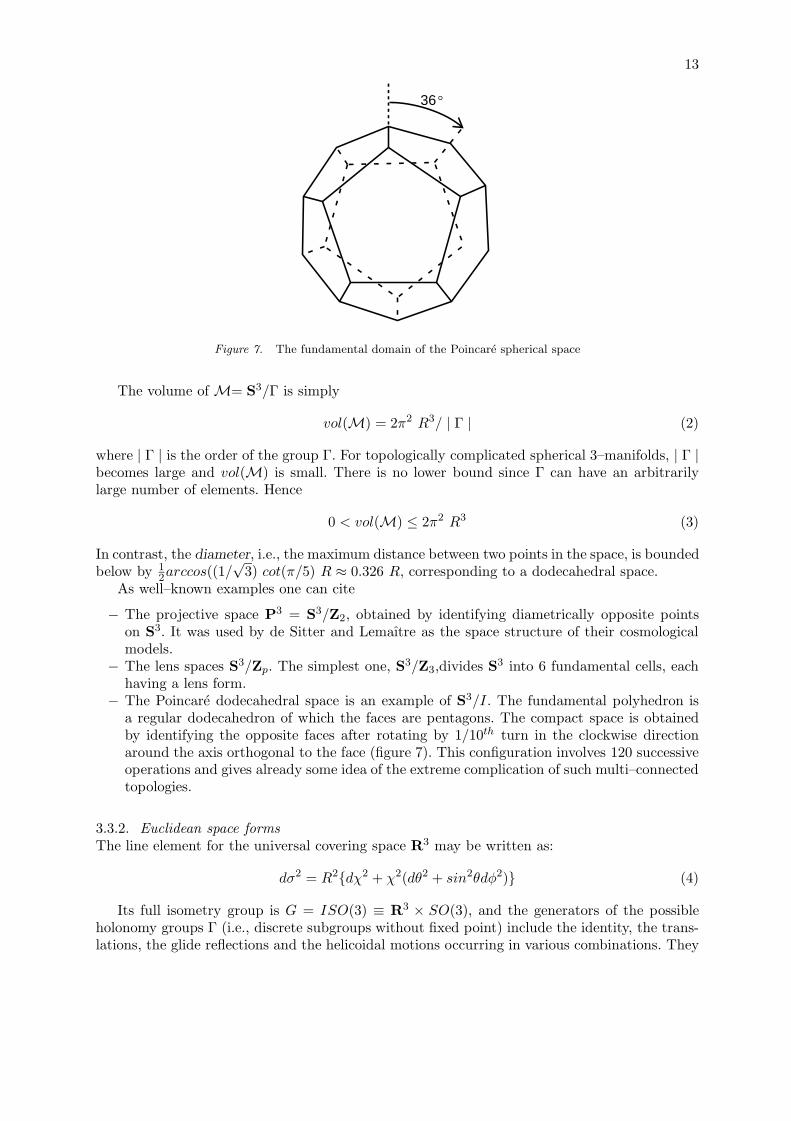
36°

Figure 7. The fundamental domain of the Poincare spherical space

The volume of M= S3/Γ is simply

vol(M) = 2π2 R3/ | Γ | (2)

where | Γ | is the order of the group Γ. For topologically complicated spherical 3–manifolds, | Γ |becomes large and vol(M) is small. There is no lower bound since Γ can have an arbitrarilylarge number of elements. Hence

0 < vol(M) ≤ 2π2 R3 (3)

In contrast, the diameter, i.e., the maximum distance between two points in the space, is boundedbelow by 1

2arccos((1/√

3) cot(π/5) R ≈ 0.326 R, corresponding to a dodecahedral space.As well–known examples one can cite

− The projective space P3 = S3/Z2, obtained by identifying diametrically opposite pointson S3. It was used by de Sitter and Lemaıtre as the space structure of their cosmologicalmodels.

− The lens spaces S3/Zp. The simplest one, S3/Z3,divides S3 into 6 fundamental cells, eachhaving a lens form.

− The Poincare dodecahedral space is an example of S3/I. The fundamental polyhedron isa regular dodecahedron of which the faces are pentagons. The compact space is obtainedby identifying the opposite faces after rotating by 1/10th turn in the clockwise directionaround the axis orthogonal to the face (figure 7). This configuration involves 120 successiveoperations and gives already some idea of the extreme complication of such multi–connectedtopologies.

3.3.2. Euclidean space formsThe line element for the universal covering space R3 may be written as:

dσ2 = R2dχ2 + χ2(dθ2 + sin2θdφ2) (4)

Its full isometry group is G = ISO(3) ≡ R3 × SO(3), and the generators of the possibleholonomy groups Γ (i.e., discrete subgroups without fixed point) include the identity, the trans-lations, the glide reflections and the helicoidal motions occurring in various combinations. They

14

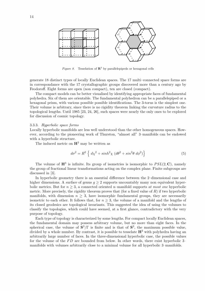
Figure 8. Tesselation of R3 by parallelepipeds or hexagonal cells

generate 18 distinct types of locally Euclidean spaces. The 17 multi–connected space forms arein correspondance with the 17 crystallographic groups discovered more than a century ago byFeodoroff. Eight forms are open (non compact), ten are closed (compact).

The compact models can be better visualised by identifying appropriate faces of fundamentalpolyhedra. Six of them are orientable. The fundamental polyhedron can be a parallelepiped or ahexagonal prism, with various possible possible identifications. The 3-torus is the simplest one.Their volume is arbitrary, since there is no rigidity theorem linking the curvature radius to thetopological lengths. Until 1985 [23, 24, 26], such spaces were nearly the only ones to be exploredfor discussion of cosmic topology.

3.3.3. Hyperbolic space formsLocally hyperbolic manifolds are less well understood than the other homogeneous spaces. How-ever, according to the pioneering work of Thurston, “almost all” 3–manifolds can be endowedwith a hyperbolic structure.

The induced metric on H3 may be written as

dσ2 = R2

dχ2 + sinh2χ (dθ2 + sin2θ dφ2)

(5)

The volume of H3 is infinite. Its group of isometries is isomorphic to PSL(2,C), namelythe group of fractional linear transformations acting on the complex plane. Finite subgroups arediscussed in [3].

In hyperbolic geometry there is an essential difference between the 2–dimensional case andhigher dimensions. A surface of genus g ≥ 2 supports uncountably many non equivalent hyper-bolic metrics. But for n ≥ 3, a connected oriented n–manifold supports at most one hyperbolicmetric. More precisely, the rigidity theorem proves that (for a fixed value of R) if two hyperbolicmanifolds, with dimension n ≥ 3, have isomorphic fundamental groups, they are necessarilyisometric to each other. It follows that, for n ≥ 3, the volume of a manifold and the lengths ofits closed geodesics are topological invariants. This suggested the idea of using the volumes toclassify the topologies, which could have seemed, at a first glance, contradictory with the verypurpose of topology.

Each type of topology is characterized by some lengths. For compact locally Euclidean spaces,the fundamental domain may possess arbitrary volume, but no more than eight faces. In thespherical case, the volume of S3/Γ is finite and is that of S3, the maximum possible value,divided by a whole number. By contrast, it is possible to tesselate H3 with polyhedra having anarbitrarily large number of faces. In the three-dimensional hyperbolic case, the possible valuesfor the volume of the FD are bounded from below. In other words, there exist hyperbolic 3–manifolds with volumes arbitrarily close to a minimal volume for all hyperbolic 3–manifolds.

15

Figure 9. Three views of the fundamental domain of the Weeks manifold

Particular interest has been taken by various authors in computing the volumes of compacthyperbolic manifolds. Each topology has a specific volume measured in curvature radius units.The absolute lower bound for the volume of CHMs is given by Vmin = 0.16668 [35]. However, itmay have little effect on cosmological applications. The reason is that the true lower bound isexpected to be 0.942707, corresponding to the smallest CHM that is presently known [85, 58].The new Vmin bound represents an improvement in the techniques of the proof, not an increasein the expected size of the smallest hyperbolic manifold.

In view of cosmological observational effects, the smaller the value of volmin, the more in-teresting the corresponding manifold for cosmology. Thus the Weeks space has been speciallystudied, by [25] and more recently by [47]. Its FD is a polyhedron with 26 vertices and 18 faces,of which 12 are pentagons and 6 are quadrilaterals. Its outer structure is represented in figure(9), the Klein coordinates of the vertices and the 18 matrix representations of the generators ofthe holonomy group are given in [47].

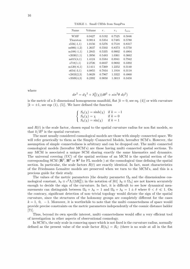
The Weeks manifold leaves room for many topological lens effects, since the volume of theobservable universe is about 200 times larger than the volume of Weeks space for Ω0 = 0.3.Indeed, many CHMs have geodesics shorter than the curvature radius, leaving room to fit agreat many copies of a fundamental polyhedron within the horizon radius, even for manifolds ofvolume ∼ 10. The publicly available program SnapPea (Weeks) is specially useful to unveil therich structure of CHMs. Several millions of CHMs with volume less than 10 could be calculated.Table 1 summarizes a sample of the results (r− is the radius of the largest sphere in the coveringspace which can be inscribed in the fundamental polyhedron, r+ is the radius of the smallestsphere in the covering space in which the fundamental polyhedron can be inscribed, lmin ≡ 2rinjis the length of the shortest geodesic; see Fig. 10).

4. Topology and Cosmology

It is presently believed that our Universe is correctly described by a perturbed Friedmann–Lemaıtre (FL) model. That is, homogeneous and isotropic solutions of Einstein’s equationsare used, of which the spatial sections have constant curvature. The observational fact thatthe Universe is, in an exact sense, inhomogeneous and anisotropic, is modelled by perturbingthese solutions. Beside the usual “big–bang” solutions, the FL models also include the de Sittersolution, as well as those incorporating a cosmological constant, or a non standard equation ofstate. From a spatial point of view, the FL models fall into 3 general classes, according to thesign of their spatial curvature k = −1, 0, or +1. The spacetime manifold is described by theRobertson–Walker metric

ds2 = c2 dt2 −R2(t) dσ2, (6)

16

TABLE 1. Small CHMs from SnapPea

Name Volume r− r+ lmin

WMF 0.9427 0.5192 0.7525 0.5846

Thurston 0.9814 0.5354 0.7485 0.5780

s556(-1,1) 1.0156 0.5276 0.7518 0.8317

m006(-1,2) 1.2637 0.5502 0.8373 0.5750

m188(-1,1) 1.2845 0.5335 0.9002 0.4804

v2030(1,1) 1.3956 0.5483 1.0361 0.3662

m015(4,1) 1.4124 0.5584 0.8941 0.7942

s718(1,1) 2.2726 0.6837 0.9692 0.3392

m120(-6,1) 3.1411 0.7269 1.2252 0.3140

s654(-3,1) 4.0855 0.7834 1.1918 0.3118

v2833(2,3) 5.0629 0.7967 1.3322 0.4860

v3509(4,3) 6.2392 0.9050 1.3013 0.3458

wheredσ2 = dχ2 + S2

k(χ)(dθ2 + sin2θ dφ2)

is the metric of a 3–dimensional homogeneous manifold, flat [k = 0, see eq. (4)] or with curvature[k = ±1, see eqs (1), (5)]. We have defined the function

Sk(χ) = sinh(χ) if k = −1Sk(χ) = χ if k = 0Sk(χ) = sin(χ) if k = 1

and R(t) is the scale factor, chosen equal to the spatial curvature radius for non flat models, sothat k/R2 is the spatial curvature.

The most usually considered cosmological models are those with simply–connected space. Wewill refer generically to them as the Simply–Connected Models, hereafter SCM’s. However, theassumption of simple–connectedness is arbitrary and can be dropped out. The multi–connectedcosmological models (hereafter MCM’s) are those having multi–connected spatial sections. Toany MCM is associated a unique SCM sharing exactly the same kinematics and dynamics.The universal covering (UC) of the spatial sections of an MCM is the spatial section of thecorresponding SCM (R3, H3 or S3 for FL models ) at the cosmological time defining the spatialsection. In particular, the scale factors R(t) are exactly identical. In fact, most characteristicsof the Friedmann–Lemaıtre models are preserved when we turn to the MCM’s, and this is aprecious guide for their study.

The values of the metric parameters [the density parameter Ω0 and the dimensionless cos-mological constant, λ0 ≡ c2Λ/(3H2

0 ); in the notation of [61] λ0 ≡ ΩΛ] are not known accuratelyenough to decide the sign of the curvature. In fact, it is difficult to see how dynamical mea-surements can distinguish between Ω0 + λ0 = 1 and Ω0 + λ0 = 1 ± δ where 0 < δ 1. Onthe contrary, significant detection of non–trivial topology would dictate the sign of the spatialcurvature, since the structures of the holonomy groups are completely different for the casesk = 1, 0, − 1. Moreover, it is worthwhile to note that the multi–connectedness of space wouldprovide precise constraints on the metric parameters independently of the cosmic distance ladder[71].

Thus, beyond its own specific interest, multi–connectedness would offer a very efficient toolof investigation in other aspects of observational cosmology.

In SCM’s, the only scale in comoving space which is not fixed is the curvature radius, normallydefined as the present value of the scale factor R(t0) = RC (there is no scale at all in the flat

17

case). Thus RC is the natural length unit in comoving space for the UC of an MCM. TheFriedmann equations imply the relation

Ω0 + λ0 − 1 =k c2

H20 R2

C

. (7)

The value of RC remains a matter of considerable debate. The only cosmological length towhich we have a direct observational access is the Hubble length

LHubble = cH−10 = 3000 h−1 Mpc.

If we define f =√| Ω + λ− 1 |, we have for a non–flat universe (for a flat universe, the value of

RC remains arbitrary):RC = LHubble f−1 = 3000 (f h)−1Mpc. (8)

In practice, the Hubble length is of the same order of magnitude as RH , the particle horizon,which defines the observable universe as a sphere in the UC. This is just slightly larger than theradius to the last scattering surface, which is the present limit to observations.

Another natural cosmological length is associated with the cosmological constant:

LΛ =√

1/Λ =√

(3H20λ0/c2)−1 = 1730/

√λ0 h−1 Mpc. (9)

The concept of horizon keeps its exact validity in the MCM’s, but must be applied to theuniversal covering space: an image is potentially visible iff its (comoving) distance is smallerthan RH in the universal covering.

In an MCM, additional spatial scales are associated with the topology, those of the fun-damental polyhedron. The geometry suggests to compare them with RC but it is often moreconvenient, for observations, to compare them to RH , or to evaluate them in Mpc or h−1 Mpc.

Figure 10 and its caption give the basic definitions. Observable effects linked to the multi–connectedness will only occur if these scales are smaller than the size of the observable universe,i.e., the horizon radius.

Dropping the hypothesis that real space is simply–connected has various implications. Ifat least one of the topological scales is smaller than the horizon, then this will, in principle,be observable: multiple images of the same object or radiation emitting region will exist. Thesmaller the fundamental domain, the easier it is to observe the multiple topological imaging.It has recently been calculated [47], for a given catalog of observable cosmic sources (discreteor diffuse) with a given depth in redshift, the approximate number of topological images inlocally hyperbolic and locally elliptic spaces as a function of the cosmological paramaters Ω0

and λ0. How do the present observational data constrain the possible multi–connectedness ofthe universe? And, more generally, what kinds of tests are conceivable ? The following sectiondeals with these matters.

5. Observational methods, candidates and constraints

5.1. “TOPOLOGY” FOR THE OBSERVER

The simplest observational point of view for approaching cosmological topology is to considerthe observable sphere, in comoving coordinates, in the covering space.

For brevity, an abuse of language is often adopted where a “topology” is considered to meana specific 3–manifold, expressed with some or all of the quantitative parameters in physical unitswith a definite orientation, in some standard astronomical coordinate system. Formally, this canbe expressed as the set

M ≡ κ0 ≡ Ω0 + λ0 − 1, Ω0, Γ, δM , δΩ0, δΓ (10)

18

rr

+-

2rinj

FP

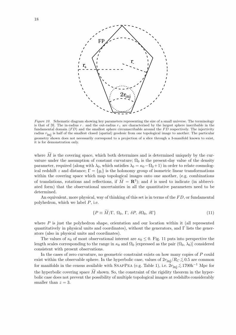
Figure 10. Schematic diagram showing key parameters representing the size of a small universe. The terminologyis that of [9]. The in-radius r− and the out-radius r+ are characterised by the largest sphere inscribable in thefundamental domain (FD) and the smallest sphere circumscribable around the FD respectively. The injectivityradius rinj is half of the smallest closed (spatial) geodesic from one topological image to another. The particular

geometry shown does not necessarily correspond to a projection of a slice through a 3-manifold known to exist,it is for demonstration only.

where M is the covering space, which both determines and is determined uniquely by the cur-vature under the assumption of constant curvature; Ω0 is the present-day value of the densityparameter, required (along with λ0, which satisfies λ0 = κ0−Ω0+1) in order to relate cosmolog-ical redshift z and distance; Γ = gi is the holonomy group of isometric linear transformationswithin the covering space which map topological images onto one another, (e.g. combinationsof translations, rotations and reflections, if M = R3); and δ is used to indicate (in abbrevi-ated form) that the observational uncertainties in all the quantitative parameters need to bedetermined.

An equivalent, more physical, way of thinking of this set is in terms of the FD, or fundamentalpolyhedron, which we label P , i.e.

P ≡ M/Γ, Ω0, Γ, δP, δΩ0, δΓ (11)

where P is just the polyhedron shape, orientation and our location within it (all representedquantitatively in physical units and coordinates), without the generators, and Γ lists the gener-ators (also in physical units and coordinates).

The values of κ0 of most observational interest are κ0 ≤ 0. Fig. 11 puts into perspective thelength scales corresponding to the range in κ0 and Ω0 [expressed as the pair (Ω0, λ0)] consideredconsistent with present observations.

In the cases of zero curvature, no geometric constraint exists on how many copies of P couldexist within the observable sphere. In the hyperbolic case, values of 2rinj/RC

<∼ 0.5 are commonfor manifolds in the census available with SnapPea (e.g. Table 1), i.e. 2rinj

<∼ 1700h−1 Mpc forthe hyperbolic covering space M shown. So, the constraint of the rigidity theorem in the hyper-bolic case does not prevent the possibility of multiple topological images at redshifts considerablysmaller than z = 3.

19

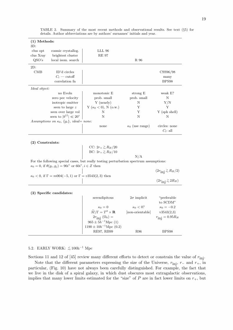
TABLE 2. Summary of the most recent methods and observational results. See text (§5) fordetails. Author abbreviations are by authors’ surnames’ initials and year.

(1) Methods:

3D:

clus opt cosmic crystallog. LLL 96

clus Xray brightest cluster RE 97

QSO’s local isom. search R 96

2D:

CMB ID’d circles CSS96/98

Cl — cutoff many

correlation fn BPS98

Ideal object:

no Evoln monotonic E strong E weak E?

zero pec velocity prob. small prob. small N

isotropic emitter Y (nearly) N Y/N

seen to large z Y (κ0 < 0), N (o.w.) Y Y

seen over large vol N Y Y (sph shell)

seen to |bII | 20 N N N

Assumptions on κ0, gi, ideal= none:

none κ0 (use range) circles: none

Cl: all

(2) Constraints:

CC: 2r+>∼RH/20

BC: 2r+>∼RH/10

N/A

For the following special cases, but really testing perturbation spectrum assumptions:

κ0 = 0, if θ(gi, gj) = 90i or 60i, i ∈ Z then

(2rinj>∼RH/2)

κ0 < 0, if Γ = m004(−5, 1) or Γ = v3543(2, 3) then

(2rinj>∼ 2RH)

(2) Specific candidates:

serendipitous 2σ implicit “preferable

to SCDM”

κ0 = 0 κ0 < 0? κ0 = −0.2

M/Γ = T 2 ×R [non-orientable] v3543(2,3)

2rinj (Ω0) = rinj = 0.95RH

965± 5h−1Mpc (1)

1190 ± 10h−1Mpc (0.2)

RE97, RB99 R96 BPS98

5.2. EARLY WORK: <∼ 100h−1 Mpc

Sections 11 and 12 of [45] review many different efforts to detect or constrain the value of rinj.Note that the different parameters expressing the size of the Universe, rinj, r− and r+, in

particular, (Fig. 10) have not always been carefully distinguished. For example, the fact thatwe live in the disk of a spiral galaxy, in which dust obscures most extragalactic observations,implies that many lower limits estimated for the “size” of P are in fact lower limits on r+, but

20

<= flat =>

CMBhorizon

Ω = 0.2, λ = 00 0

H-1~R ~ 9700 h Mpc

horizon

-1

Ω = 0.2, λ = 0.80 0

HR ~ 11700 h Mpc~

H

Ω = 1, λ = 00 0

horizon

-1R = 6000 h Mpc

R = "infinity"

R = "infinity"C

C

CR = 3354 h Mpc-1

z=3z=0.5

z=3 z=3

z=0.5z=0.5

=>

hyperbolic

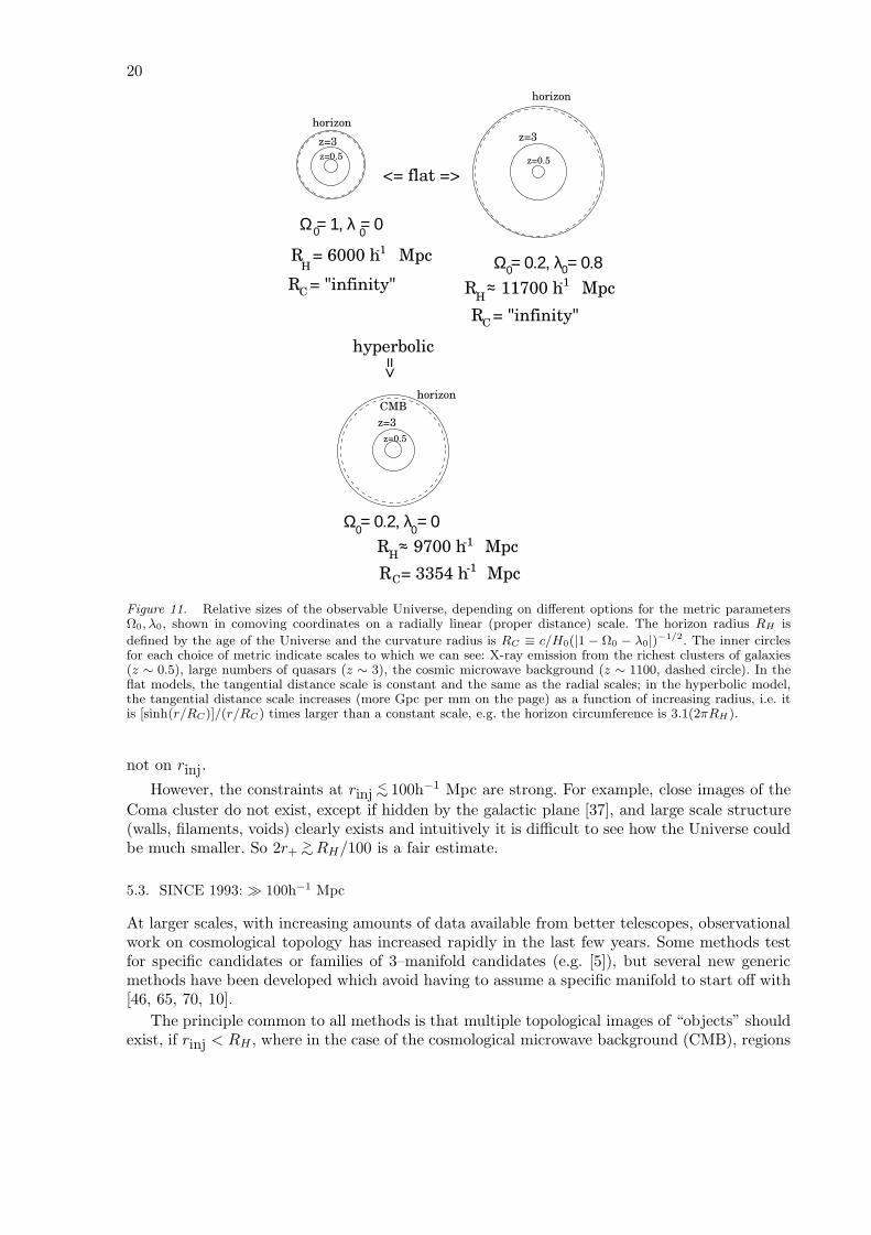
Figure 11. Relative sizes of the observable Universe, depending on different options for the metric parametersΩ0, λ0, shown in comoving coordinates on a radially linear (proper distance) scale. The horizon radius RH is

defined by the age of the Universe and the curvature radius is RC ≡ c/H0(|1 − Ω0 − λ0|)−1/2. The inner circlesfor each choice of metric indicate scales to which we can see: X-ray emission from the richest clusters of galaxies(z ∼ 0.5), large numbers of quasars (z ∼ 3), the cosmic microwave background (z ∼ 1100, dashed circle). In theflat models, the tangential distance scale is constant and the same as the radial scales; in the hyperbolic model,the tangential distance scale increases (more Gpc per mm on the page) as a function of increasing radius, i.e. itis [sinh(r/RC)]/(r/RC ) times larger than a constant scale, e.g. the horizon circumference is 3.1(2πRH ).

not on rinj.

However, the constraints at rinj<∼ 100h−1 Mpc are strong. For example, close images of the

Coma cluster do not exist, except if hidden by the galactic plane [37], and large scale structure(walls, filaments, voids) clearly exists and intuitively it is difficult to see how the Universe couldbe much smaller. So 2r+

>∼RH/100 is a fair estimate.

5.3. SINCE 1993: 100h−1 Mpc

At larger scales, with increasing amounts of data available from better telescopes, observationalwork on cosmological topology has increased rapidly in the last few years. Some methods testfor specific candidates or families of 3–manifold candidates (e.g. [5]), but several new genericmethods have been developed which avoid having to assume a specific manifold to start off with[46, 65, 70, 10].

The principle common to all methods is that multiple topological images of “objects” shouldexist, if rinj < RH , where in the case of the cosmological microwave background (CMB), regions

21

O

S

S1 S2 S3

S4 S5

S6 S7 S8

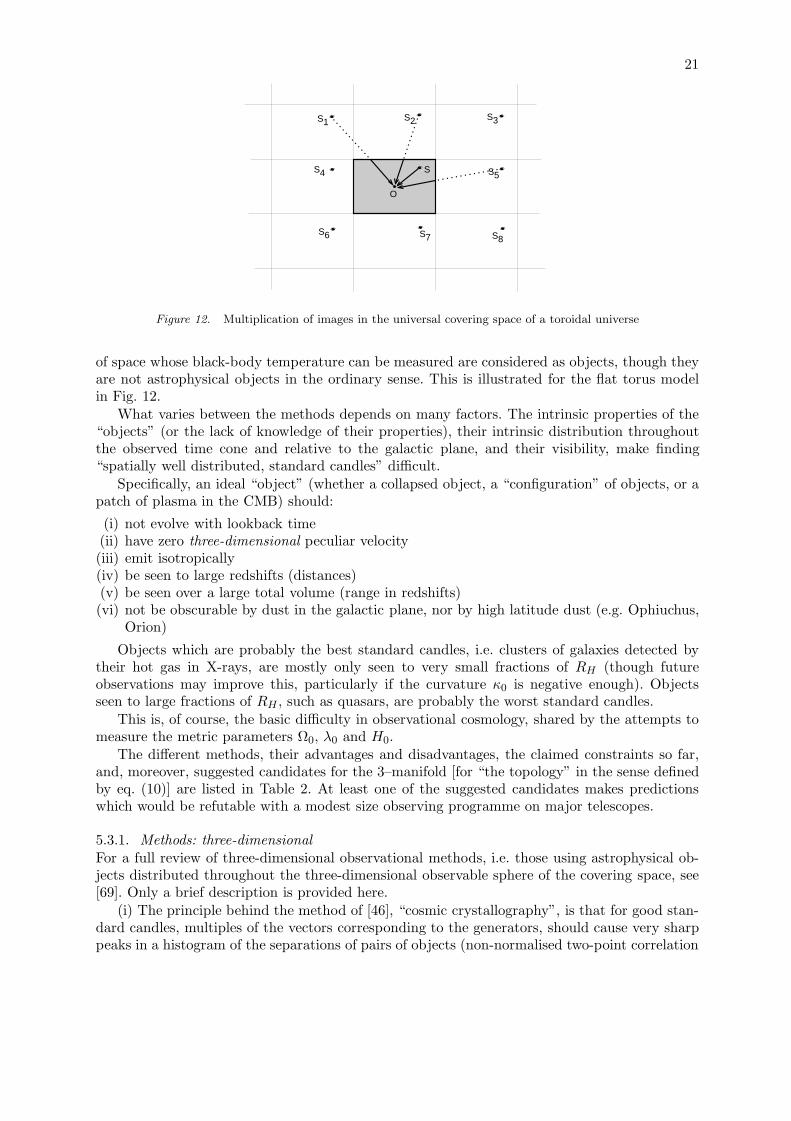
Figure 12. Multiplication of images in the universal covering space of a toroidal universe

of space whose black-body temperature can be measured are considered as objects, though theyare not astrophysical objects in the ordinary sense. This is illustrated for the flat torus modelin Fig. 12.

What varies between the methods depends on many factors. The intrinsic properties of the“objects” (or the lack of knowledge of their properties), their intrinsic distribution throughoutthe observed time cone and relative to the galactic plane, and their visibility, make finding“spatially well distributed, standard candles” difficult.

Specifically, an ideal “object” (whether a collapsed object, a “configuration” of objects, or apatch of plasma in the CMB) should:

(i) not evolve with lookback time(ii) have zero three-dimensional peculiar velocity(iii) emit isotropically(iv) be seen to large redshifts (distances)(v) be seen over a large total volume (range in redshifts)(vi) not be obscurable by dust in the galactic plane, nor by high latitude dust (e.g. Ophiuchus,

Orion)

Objects which are probably the best standard candles, i.e. clusters of galaxies detected bytheir hot gas in X-rays, are mostly only seen to very small fractions of RH (though futureobservations may improve this, particularly if the curvature κ0 is negative enough). Objectsseen to large fractions of RH , such as quasars, are probably the worst standard candles.

This is, of course, the basic difficulty in observational cosmology, shared by the attempts tomeasure the metric parameters Ω0, λ0 and H0.

The different methods, their advantages and disadvantages, the claimed constraints so far,and, moreover, suggested candidates for the 3–manifold [for “the topology” in the sense definedby eq. (10)] are listed in Table 2. At least one of the suggested candidates makes predictionswhich would be refutable with a modest size observing programme on major telescopes.

5.3.1. Methods: three-dimensionalFor a full review of three-dimensional observational methods, i.e. those using astrophysical ob-jects distributed throughout the three-dimensional observable sphere of the covering space, see[69]. Only a brief description is provided here.

(i) The principle behind the method of [46], “cosmic crystallography”, is that for good stan-dard candles, multiples of the vectors corresponding to the generators, should cause very sharppeaks in a histogram of the separations of pairs of objects (non-normalised two-point correlation

22

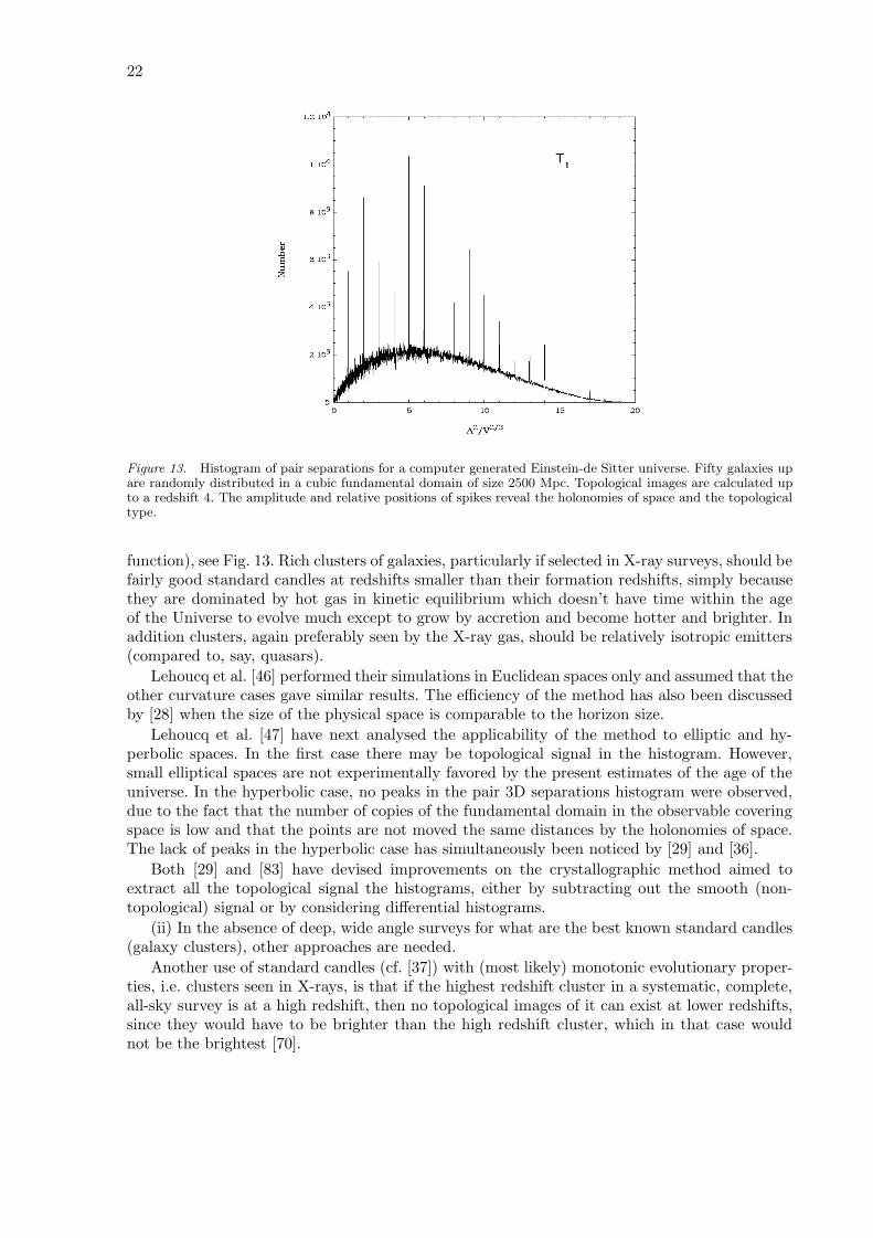
Figure 13. Histogram of pair separations for a computer generated Einstein-de Sitter universe. Fifty galaxies upare randomly distributed in a cubic fundamental domain of size 2500 Mpc. Topological images are calculated upto a redshift 4. The amplitude and relative positions of spikes reveal the holonomies of space and the topologicaltype.

function), see Fig. 13. Rich clusters of galaxies, particularly if selected in X-ray surveys, should befairly good standard candles at redshifts smaller than their formation redshifts, simply becausethey are dominated by hot gas in kinetic equilibrium which doesn’t have time within the ageof the Universe to evolve much except to grow by accretion and become hotter and brighter. Inaddition clusters, again preferably seen by the X-ray gas, should be relatively isotropic emitters(compared to, say, quasars).

Lehoucq et al. [46] performed their simulations in Euclidean spaces only and assumed that theother curvature cases gave similar results. The efficiency of the method has also been discussedby [28] when the size of the physical space is comparable to the horizon size.

Lehoucq et al. [47] have next analysed the applicability of the method to elliptic and hy-perbolic spaces. In the first case there may be topological signal in the histogram. However,small elliptical spaces are not experimentally favored by the present estimates of the age of theuniverse. In the hyperbolic case, no peaks in the pair 3D separations histogram were observed,due to the fact that the number of copies of the fundamental domain in the observable coveringspace is low and that the points are not moved the same distances by the holonomies of space.The lack of peaks in the hyperbolic case has simultaneously been noticed by [29] and [36].

Both [29] and [83] have devised improvements on the crystallographic method aimed toextract all the topological signal the histograms, either by subtracting out the smooth (non-topological) signal or by considering differential histograms.

(ii) In the absence of deep, wide angle surveys for what are the best known standard candles(galaxy clusters), other approaches are needed.

Another use of standard candles (cf. [37]) with (most likely) monotonic evolutionary proper-ties, i.e. clusters seen in X-rays, is that if the highest redshift cluster in a systematic, complete,all-sky survey is at a high redshift, then no topological images of it can exist at lower redshifts,since they would have to be brighter than the high redshift cluster, which in that case wouldnot be the brightest [70].

23

(iii) At larger scales, the objects most readily available are quasars. These are not goodstandard candles, and either exist (as quasars) only for small fractions of the age of the Universe,or recur as bursts several times. In addition, they would be seen (except in special cases) fromdifferent angles, and so appear as another form of active galactic nucleus (AGN) much fainter,and not yet catalogued.

The way around this problem [65] is to look for, in a large enough catalogue, the rare casesin which the evolution (and orientation) of the quasars happens to be ideal for an Earth-basedobserver, and multiple topological images are seen of several quasars in two topological imagesof a “small region”, i.e. of a region of a few 100h−1 Mpc in size. The method is then to search (in3-D, using redshifts for distance estimation) for all possible isometries between configurationsof quasars in such “small regions”. There is not much time for the relative positions of quasarsto change much within a configuration, so in a sense, the configurations correspond to pseudo-objects of size 100h−1 Mpc which, in a small number of cases, effectively do not evolve.

Given contamination by chance isometries of configurations unrelated to topology [65], the-oretical work (analytical and/or simulations) is required to find the statistically optimal imple-mentations of this method. For example, although weakening the isometry criteria (e.g. matchingquadruplets instead of quintuplets) would increase the number of non-topological (noise) isome-tries, it might increase the number of topological (signal) matches by a greater factor.

(iv) A method not yet applied directly, though implicit in some sense in the above methods,is to consider units of “large scale structure” (walls, voids, etc. on scales of 50–150h−1 Mpc) asobjects. Although individual galaxies and quasars will be difficult to identify at different epochs,it is expected that they should trace out thin structures which should not move much over thetime scales involved [37]. One approach to analysing the data to be taken by the X-ray satelliteXMM is to use the representations of large scale structure by the 2-dimensional topology ofcontours of constant density as a characteristic to identify potential multiple topological imagesof these structures. In other words, the (2-D) topology of matter would be used to search forthe (3-D) topology of space [62].

(v) Other methods to note include [23, 24, 26] specifically for the hyperbolic case and [27]for looking for images of our own galaxy as a quasar. In fact, a challenge to the astronomers andastrophysicists who try understand the dynamical, inter-stellar medium (ISM) and stellar pasthistory of the Milky Way (MW) and Local Group galaxies (LG) is that they should be able todescribe this history in a unique enough fashion such that high redshift galaxies can be excludedas possible topological images of the Milky Way just on the basis of intrinsic properties, ratherthan on checking for further topological images.

Since this school is intended for doctoral (graduate) students, it should be pointed out thatthis would provide a “safe” thesis project with relevance for cosmic topology, in that the maingoal would be to understand the history of the MW and LG, which is already more than enoughfor a thesis. If it resulted that a “high” redshift galaxy (or a group) were found to have a strikingresemblance to how the MW (or LG) should have looked at that epoch, then the student wouldnot necessarily need to conclude that topological images have been found — the resemblancecould be ascribed to coincidence and checked for cosmological significance during postdoctoralwork (or by other researchers in the field). However, the advances in the understanding of theMW and LG history in order to make such a significant claim of resemblance would be sufficientfor several publishable articles.

5.3.2. Methods: two-dimensionalThe principle behind the use of the CMB, i.e. of a nearly two-dimensional thin shell from theobserver’s point of view, is that small portions of the shell corresponding to the CMB can beconsidered in some sense as objects. Depending on the topology of the Universe, some of these“objects” may occupy points of space which have topological images on other parts of the CMB.

24

FD FD

universal covering space

FD (fundamental domain)

zoom in

zoom in

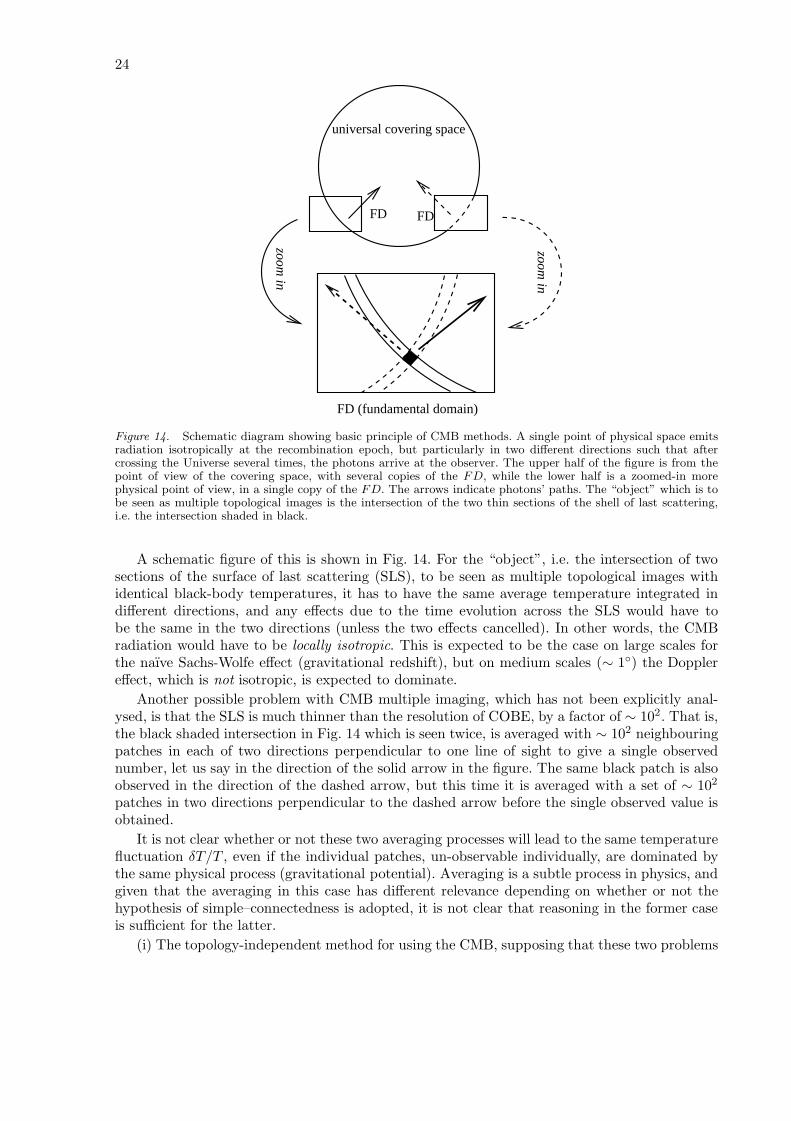
Figure 14. Schematic diagram showing basic principle of CMB methods. A single point of physical space emitsradiation isotropically at the recombination epoch, but particularly in two different directions such that aftercrossing the Universe several times, the photons arrive at the observer. The upper half of the figure is from thepoint of view of the covering space, with several copies of the FD, while the lower half is a zoomed-in morephysical point of view, in a single copy of the FD. The arrows indicate photons’ paths. The “object” which is tobe seen as multiple topological images is the intersection of the two thin sections of the shell of last scattering,i.e. the intersection shaded in black.

A schematic figure of this is shown in Fig. 14. For the “object”, i.e. the intersection of twosections of the surface of last scattering (SLS), to be seen as multiple topological images withidentical black-body temperatures, it has to have the same average temperature integrated indifferent directions, and any effects due to the time evolution across the SLS would have tobe the same in the two directions (unless the two effects cancelled). In other words, the CMBradiation would have to be locally isotropic. This is expected to be the case on large scales forthe naıve Sachs-Wolfe effect (gravitational redshift), but on medium scales (∼ 1) the Dopplereffect, which is not isotropic, is expected to dominate.

Another possible problem with CMB multiple imaging, which has not been explicitly anal-ysed, is that the SLS is much thinner than the resolution of COBE, by a factor of ∼ 102. That is,the black shaded intersection in Fig. 14 which is seen twice, is averaged with ∼ 102 neighbouringpatches in each of two directions perpendicular to one line of sight to give a single observednumber, let us say in the direction of the solid arrow in the figure. The same black patch is alsoobserved in the direction of the dashed arrow, but this time it is averaged with a set of ∼ 102

patches in two directions perpendicular to the dashed arrow before the single observed value isobtained.

It is not clear whether or not these two averaging processes will lead to the same temperaturefluctuation δT/T , even if the individual patches, un-observable individually, are dominated bythe same physical process (gravitational potential). Averaging is a subtle process in physics, andgiven that the averaging in this case has different relevance depending on whether or not thehypothesis of simple–connectedness is adopted, it is not clear that reasoning in the former caseis sufficient for the latter.

(i) The topology-independent method for using the CMB, supposing that these two problems

25

can be overcome, is the “method of circles” [10, 86]. Consider extending the tiling of the coveringspace by copies of the FD beyond the observable sphere and consider the observable sphere ofa second observer in one of the copies of the FD outside the first sphere. The intersection ofthese two spheres is a circle.

But since each copy of the FD is equivalent, the second observer can in fact perfectly wellbe physically identical with the first observer. That is, in the covering space, two observers, eachof to whom the other is behind the CMB (but not too far), are equivalent to a single observerlooking in two different directions towards the CMB, as long as they are at the same positionwithin the FD.

Hence, the effect of multi-connectedness would be that the values of the temperature fluctu-ations δT/T around certain circles on the CMB would map onto one another, since the circlescorrespond to the same set of points in space and time.

A related two-dimensional method to be applied to future satellites (MAP and Planck Sur-veyor), is that of searching for patterns of hot and cold spots [53]. This may bypass the problemof the large number of calculations to make for the circles method.

(ii) Other two-dimensional methods require (a) assuming the topology and specific quantita-tive parameters for individual 3–manifolds of each given topology and (b) modelling the powerspectrum of perturbations. The latter is difficult to justify.

The theoretical motivation for Gaussian amplitude distributions, uniform random phasesand a P (k) ∝ k1 power spectrum are unlikely to be valid at scales approaching rinj and r+.That is, either for a hyperbolic or for a flat, λ0 ∼ 0.7 metric to be presently observable, inflationneeds some degree of fine-tuning (which can partly be provided by the ergodicity of geodesics inthe former case, [8]). Since curvature or λ0 > 0 must remain “uninflated” in the sense of beingobservable at the present epoch in these cases, it is unclear why perturbations on the scale ofRC ∼ RH should necessarily be “inflated” in the sense of exactly satisfying the assumptions onthe power spectrum. Moreover, even for other choices of metric, if the Universe is observably anMCM, then scales approaching rinj and r+ need not necessarily be “inflated” either.

The observational motivation for Gaussian amplitude distributions, uniform random phasesand a P (k) ∝ k1 power spectrum are equally lacking for tests of MCM’s. The only observationaljustification of these properties on large scales is COBE data, which is analysed assuming simple–connectedness. A self-consistent assumption on the fluctuation spectrum for comparison of anMCM with COBE data would be to calculate this spectrum in three dimensions based on theCOBE data shifted into the FD of the MCM assumed. However, use of the resultant spectrumto simulate properties of the COBE observations would give . . . exactly the COBE observations(if it has been done correctly).

So a self-consistent alternative to (b) would not enable rejection of an MCM. In other words,this approach tests assumptions on the the fluctuation spectrum (on the scale <∼ rinj < r+)rather than the MCM itself. (Moreover, some authors find violation of Gaussian amplitudedistributions in the COBE data [31, 60].)

Nevertheless, approach (ii) has been applied several times. Generally, a spherical harmonicanalysis (“Cl” spectrum) of simulated CMB maps (e.g. [78, 77]) is calculated.

For a hyperbolic spatial section, a standard Fourier analysis is, in a strict sense, invalid,whether or not a trivial topology is assumed. This compounds the problems of assumptionsregarding the power spectrum, which cannot be defined in the usual way. Moreover, the classifi-cation and listing of the 3–manifolds is an open enough problem, and knowledge of eigenmodesfor the equivalent of a Fourier analysis is even less developed. An interesting way to avoid thisproblem is to use correlation functions rather than power spectra for assumption (b). Bond,Pogosyan & Souradeep [5] have done this for two of the many hyperbolic 3–manifolds known.

A general argument claimed for the methods which assume specific 3–manifolds is that noobjects, i.e. no density fluctuations, which are larger than the Universe, i.e. larger than r+, can

26

exist, so there should be a cutoff at small l values (large length scales) in the Cl spectrum.While this may sound common sense, it is only correct in the FD. In the universal covering

space, fluctuations much larger than the Universe can indeed exist (e.g. ∼ 30 times larger,see Fig. 1 of [65]). These structures cross the FD many times. While the Cl spectrum mayindeed lose power on large scales due to averaging in different directions, it is incorrect to statethat fluctuations larger than r+ cannot exist. The component eigenmodes in 3-D are of courseconstrained by some integer multiple of r+, but basis functions of the 2-D sphere cut to ±20from the galactic plane only relate to the 3-D eigenmodes via simplifying assumptions whichonce again may not be valid at these length scales in MCM’s. Recently Inoue [40] computed thelow-lying eigenmodes on some compact 3-hyperbolic spaces using the direct boundary elementmethod, and found that the expansion coefficients behave as gaussian pseudo-random numbers.

A summary of the advantages and disadvantages of these different methods is shown in thefirst part of Table 2.

Another interesting constraint may be derived when we take into account the possibilitythat phase transitions in the early universe could develop topological defects. Uzan & Peter [84]showed that if space is multi–connected on scales now smaller than the horizon size, stringsand domain walls were very unlikely to exist. Uzan [81, 82] generalized these results to texturesand studied the cosmological implications of such constraints. He concluded that a large classof multi-connected universes with topological defects accounting for structure formation wereruled out by the cosmic microwave background observations.

5.3.3. Constraints3-D (i,ii) The cosmic crystallography ([46], CC) and brightest cluster ([70], BC) methods indicatelower limits on the out-diameter of around RH/20 and RH/10 respectively, though the formeris valid only in Euclidean spaces R3/Γ.

3-D (iii) The isometry search method applied to quasars is specifically designed to work forpoor standard candles, so is intended for finding specific candidates for the 3–manifold, not forconstraining rinj or r+.

2-D (i) No application of the identified circles principle to COBE data to constrain rinj orr+ has yet been published, since the poor signal-to-noise and resolution make the chance of adetection seem unlikely.

2-D (ii) However, many applications of the two-dimensional methods to observations fromthe COBE satellite [78, 77, 42, 13, 52, 5] have been made. These can be interpreted eitheras suggesting constraints close to the horizon scale, but only for a (mostly Euclidean) finitenumber of the infinitely many topologies possible, or as showing that standard assumptions onthe statistics of the perturbation spectrum on scales close to rinj and r+ would have to be wrongfor one of these MCM’s to be correct. Note that the confidence limits stated for several of thesestudies are statements about the distribution of random realisations, not about observationalinconsistency of multiply imaged observed patches of the CMB.

These various direct constraints and perturbation spectrum based tests are listed in thesecond part of Table 2.

The poor resolution of COBE (∼ 10) implies that the data from the MAP and Plancksatellites will probably be necessary before the circles principle can be applied seriously. Thiswill not be easy, due to the Doppler effect, the integrated Sachs-Wolfe effect, other foregrounds,and the problem of averaging mentioned above.

5.3.4. Specific candidatesThe most specific candidates suggested are those of [70] and [5], though an implicit candidatemay also be implied by the application of the isometry search method to quasars [65].

27

The former candidate was noticed by chance in a small list of some of the brightest clusterschosen to illustrate the brightest cluster method. Among these seven clusters, three form a rightangle to within 2%-3% accuracy (depending on the values of Ω0 and λ0) and the two side lengthsadjacent to the near-right angle are equal to within 1%. This is better than tolerance consideredfor special quasar configurations by [27].

An a posteriori estimate of the probability of this occurring by chance would be difficult tomake objectively, but since the configuration

(i) corresponds to that expected for the most commonly studied candidate in CMB studies(variations on hypertori),

(ii) implies generators which can easily be used to derive observationally refutable predictions,and

(iii) can be used to test in detail the validity of the different statistical methods,

it is useful to consider the implied M/Γ = T 2 ×R as a candidate 3.See [70] for object names, positions and values of the generators. A more recent summary of

arguments for and against the candidate is provided in the discussion section of [68]; see also [66]for a COBE analysis. If the candidate were correct, then two topological images of the Comacluster would be already known.

Bond et al. [5] (1998, §4.3) have also noticed a 3–manifold (for the two hyperbolic topologiesconsidered) which, for a certain orientation, is “preferable to standard cold dark matter” whencompared to the COBE observations. The volume of this manifold is slightly larger that thatof the observable sphere, but rinj is less than RH , though not enough to imply any multipletopological images at observable sub-SLS distances.

5.4. OTHER OBSERVATIONAL DIFFICULTIES

Another observational complication, which has not generally been considered, particularly inthe claims of constraints, i.e. lower limits on rinj, is an important point by [22]: in a strict sense,it is already well established that we do not live in an FL universe. We live in what (locally, atleast) is an almost FL universe. Density perturbations (humans, planets, stars, galaxies, largescale structure) exist.

Depending on the way in which space inside the observable sphere and the FD differs froman exact FL universe, the real spatial geodesics will not correspond exactly to multiples (andsums) of the generators derived assuming an exact FL universe. Gravitational lensing is oneexample, though the effect is probably small.

6. Conclusion

The present surge of research in the mathematics, the physical theory and the observations ofcosmological topology promise exciting developments in all three fields. Moreover, some of thespin-offs which would follow from a significant detection have been explicitly calculated: themeasurement of transversal galaxy velocities [68], precise estimates of the metric parameters[71], position of the topological signature in the Ω0–λ0 plane [83].

Mathematics: Continued work by mathematicians to understand and classify hyperbolic 3–manifolds may help theorists develop ideas regarding the physics behind global topology, whilefurther developments in the software (SnapPea) will be useful to observational astronomers.

Theory: The development of predictions by quantum gravity theories before a 3–manifoldcandidate is confirmed to high significance would be useful from an epistemological point ofview.

28

Observations: The numerous observational methods offer plenty of scope for improvements inthe practical details while waiting for new surveys such as the SDSS (Sloan Digital Sky Survey)and new satellites such as XMM (X-ray Multiple Mission), MAP and Planck Surveyor.

However, it is not necessary to wait: specific candidates for the 3–manifold have been andshould continue to be proposed. The benevolence of time allocation committees for the ob-servational refutation (or strengthening) of the candidates should contribute significantly toobservational cosmo-topology.

References

1. Atkatz, D., Pagels, H., 1982, Phys. Rv. D 25, 20652. Barbour J. & Pfister H., 1995, (Eds.) Mach’s Principle: From Newton’s Bucket to Quantum Gravity (Einstein

Studies, Vol 6), Birkhauser3. Beardon, A.F. 1983, The Geometry of Discrete Groups (GTM91) New York:Springer4. Bieberbach, L., 1911, Mathematische Annalen, 70,297. 1912; Ibid, 72, 400.5. Bond J. R., Pogosyan D., Souradeep T., 1998, Class.Quant.Grav., 15, 2573 (astro-ph/9804041)6. Briel U. G., Henry J. P., Bohringer H., 1992, A&A, 259, L317. Carlip S., 1998, Class.Quant.Grav., 15, 2629 (gr-qc/9710114)8. Cornish N. J., Spergel D. N., Starkman G. D., 1996, Phys.Rev.Lett., 77, 2159. Cornish N. J., Spergel D. N., Starkman G. D., 1998a, astro-ph/970822510. Cornish N. J., Spergel D. N., Starkman G. D., 1998b, Class.Quant.Grav., 15, 2657 (astro-ph/9801212)11. da Costa L. N., in Cosmic Velocity Fields, ed. Bouchet F., Lachieze-Rey M., (Gif-sur-Yvette, France: Editions

Frontieres), p.47512. Dekel, A., Burnstein, D., White, S., 1996, in Critical Dialogues in Cosmology, ed. N.Turok, World Scientific.13. de Oliveira Costa A., Smoot G. F., 1995, Ap.J., 448, 47714. de Sitter W., 1917, MNRAS, 78, 315. Dowker H. F., Garcia R. S., 1998, Class.Quant.Grav., 15, 1859 (gr-qc/9711042)16. Dowker H. F., Surya S., 1998, PhysRevD, 58, 124019 (gr-qc/9711070)17. e Costa S. S., Fagundes H. V., 1998, gr-qc/980106618. Einstein, A., Postcard to Hermann Weyl, June 1918, from Einstein Archives, Princeton (freely translated

from German by J.-P. Luminet).19. Einstein, A., 1919, Postcard to Kelix Klein, April 16th, ibid.20. Einstein, A., de Sitter W., 1932, Proc. Nat. Acad. Sci 18, 213.21. Ellis, G.F.R. 1971, Gen.Rel.Grav. 2, 722. Ellis G.F.R., Schreiber, G., 1986, PhysLettA, 115, 9723. Fagundes H. V., 1985, Ap.J., 291, 45024. Fagundes H. V., 1989, Ap.J., 338, 61825. H.V. Fagundes, 1993, Phys. Rev. Lett. 70, 157926. Fagundes H. V., 1996, Ap.J., 470, 4327. Fagundes H. V., Wichoski U. F., 1987, Ap.J., 322, L528. Fagundes, H. & Gausmann, E., 1997, On Closed Einstein-de Sitter Universes, astro-ph/9704259.29. Fagundes, H. & Gausmann, E., 1999, astro-ph/981136830. Feodoroff, E., 1885, Russian journal for crystallography and mineralogy, St Petersburg, 21.31. Ferreira P. G., Magueijo J., Gorski K. M., 1998, Ap.J., 503, L132. Friedmann, A., 1922, Zeitschrift fur Physik, 10, 37.33. Friedmann, A., 1923, Mir kak prostranstvo i vremya (The Universe as Space and Time), Leningrad,

Akademiya (French translation in Essais de Cosmologie, Le Seuil/Sources du Savoir, Paris, 1997.)34. Friedmann A., 1924, Zeitschr.fur Phys., 21, 32635. Gabai, D. Meyerhoff, R., Thurston, N., 1996, Homotopy Hyperbolic 3–manifolds Are Hyperbolic, preprint

available at http://www.msri.org/MSRI-preprints/online/1996-058.html36. Gomero, G. I., Teixeira, A. F. F., Reboucas, M. J., Bernui, A., 1999, gr-qc/981103837. Gott J. R., 1980, MNRAS, 193, 153

1986, in Inner Space/Outer38. Harrison, E., 1987, Darkness at night, Harvard University Press.39. Hawking S., 1984, NuclPhysB, 239, 25740. Inoue, K.T., astro-ph/9810034.41. Ionicioiu R., 1998, gr-qc/971106942. Jing Y.-P., Fang L.-Z., 1994, PhysRevLett, 73, 1882 (astro-ph/9409072)43. Klein, F., 1890, Mathematisches Annalen, 37, 544.44. Killing, W., 1891, Mathematisches Annalen, 39, 257.45. Lachieze-Rey M., Luminet J.-P., 1995, PhysRep, 254, 13646. Lehoucq R., Luminet J.-P., Lachieze-Rey M., 1996, A&A, 313, 33947. Lehoucq R., Luminet J.-P., Uzan J.-Ph., 1999, A&A, to be published (astro-ph/9811107)

29

48. Lemaıtre, G., 1927, Ann. Soc. Sci. Bruxelles, ser. A, 47, 29.49. Lemaıtre, G., 1931, MNRAS 90, 490.50. Lemaıtre G., 1958, in La Structure et l’Evolution de l’Univers, Onzieme Conseil de Physique Solvay, ed.

Stoops R., (Brussels: Stoops), p.151. Lemaıtre, G., 1978 (posth.) in L’Univers, probleme accessible a la science humaine, Revue d’Histoire Scien-

tifique, 31, pp. 345-359.52. Levin J., Scannapieco E., Silk J., 1998, Class.Quant.Grav., 15, 268953. Levin J., Scannapieco E., de Gasperis, G., Silk J., Barrow, J.D., 1998, astro-ph/980720654. Luminet, J.-P., 1997 L’invention du big bang, suivi de A. Friedmann, G. Lemaıtre : Essais de Cosmologie

(Le Seuil/Sources du Savoir, Paris).55. Luminet, J.-P., 1998, Acta Cosmologica, 24 (gr-qc/9804006)56. Luminet, J.-P. & Lachieze-Rey, M., 1994, La physique et l’infini (Flammarion/Dominos, Paris).57. Madore J., Saeger L. A., 1998, Class.Quant.Grav., 15, 811 (gr-qc/9708053)58. Matveev S.V., Fomenko A.T., 1988, Russian Math. Surveys 43, 3.59. Novacki, W., 1934, Commentarii Mathematici Helvetici, 7, 81.60. Pando, J., Valls-Gabaud, D., Fang, L.-Zh., 1998, PhysRevLett, accepted, (astro-ph/9810165)61. Peebles, P.J.E., 1993, Principles of Physical Cosmology, Princeton, U.S.A.: Princeton Univ. Press62. Pierre, M., 1999, Proceedings of the workshop Cosmological Topology in Paris 1998 (Obs. Paris/IAP, Paris

14 December 1998), http://www.iap.fr/users/roukema/CTP98/resumes.html63. Rainer M., 1996, gr-qc/9602059.64. Rosales J.-L., 1998, gr-qc/971205965. Roukema B. F., 1996, MNRAS, 283, 114766. Roukema B. F., 1999, submitted67. Roukema, B. F. et al., 1999, Proceedings of the workshop Cosmological Topology in Paris 1998 (Obs.

Paris/IAP, Paris 14 December 1998), http://www.iap.fr/users/roukema/CTP98/resumes.html68. Roukema B. F., Bajtlik, S., 1999, submitted to MNRAS69. Roukema B. F., Blanloeil V., 1998, Class.Quant.Grav., 15, 2645 (astro-ph/9802083)70. Roukema B. F., Edge A. C., 1997, MNRAS, 292, 10571. Roukema B. F., Luminet, J.-P., 1999, submitted72. Schwarzschild, K. Vierteljahrschrift der Ast. Ges. 35 67, 190073. Schwarzschild, K., 1998, Class.Quant.Grav., 15, 2539 [english translation of Schwarzschild (1900)]74. Spaans, M., 1999, gr-qc/990102575. Starkman G. D., 1998, Class.Quant.Grav., 15, 252976. Starkman, G. et al., 1998, Invited papers from the workshop Cosmology and topology (CWRU, Cleveland,

25-27 October 1997), Class. Quant. Grav. 15, 252977. Starobinsky A. A., 1993, JETPLett, 57, 62278. Stevens D., Scott, Silk J., 1993, PhysRevLett, 71, 2079. Thurston, W. P., 1979, The geometry and topology of three manifolds, (Princeton Lecture Notes)80. Thurston, W. P., 1997, Three-Dimensional Geometry and Topology, ed. Levy, S., Princeton, U.S.A.: Prince-

ton University Press81. J-Ph. Uzan, 1998a, Phys. Rev. D58, 08730182. J-Ph. Uzan, 1998b, Class. Quant. Grav. 15, 271183. Uzan J.-Ph., Lehoucq R., Luminet J.-P., 1999, in preparation84. Uzan, J.-Ph., Peter P., 1997, Phys.Lett. B 406, 2085. Weeks, J., 1985, PhD thesis, Princeton University.86. Weeks J. R., 1998, Class.Quant.Grav., 15, 2599 (astro-ph/9802012)87. Wolf, J.A., 1960, C. R. Acad. Si. Paris,250, 3443.88. Zel’dovich Y. B., Grishchuk L. P., 1984, MNRAS, 207, 23P