Page 1
Department of Construction Sciences
Solid Mechanics
ISRN LUTFD2/TFHF-17/5222-SE(1-60)
Topology Optimization forAdditive Manufacturing
Master’s Dissertation by
Kajsa Soderhjelm
Supervisor:Mathias Wallin
Examiner:Ralf Denzer
Copyright c© 2017 by the Division of Solid Mechanicsand Kajsa Soderhjelm
Printed by Media-Tryck AB, Lund, SwedenFor information, address:
Division of Solid Mechanics, Lund University, Box 118, SE-221 00 Lund, SwedenWebpage: www.solid.lth.se
Page 3
Acknowledgement
This master thesis is submitted for a Master's Degree in Mechanical Engineering at the
Division of Solid Mechanics, Faculty of Engineering, Lund University.
I would rst like to thank my supervisor Professor Mathias Wallin for his guidance and
many discussions, this thesis would not exist without his expertise in the eld or enthu-
siasm for research. I would like to thank Niklas Ivarsson for all the help and discussions,
especially during our trip to Dalian University of Technology in China. I would also like
to thank Professor Jun Yan and Professor Bin Niu at the Dalian University of Technology
for their expertise, help, and kind welcoming to China.
Lastly but just as important, I want to thank my dear Björn, my parents and all of
my friends for all the love and support.
Lund, November 2017
Kajsa Söderhjelm
Page 5
Abstract
Topology optimization answers the question "How to place the material within a pre-
scribed design domain in order to obtain the best structural performance?" and the design
obtained is usually complex. Additive manufacturing comes with a well known design
freedom and the design provided by topology optimization can be manufactured without
as many constraints as conventional manufacturing methods. However, there does exist a
few constraints that needs to be considered such as minimum feature size, enclosed voids,
and overhang. This work focus on overcoming the overhang constraint.
A new method proposed by Langelaar (2017) solved with the optimality criteria with a
density lter provides printable structures regarding the overhang constraint. The method
is very computationally ecient, but the overhang angle is tied to the element discretiza-
tion and the printing direction needs to be axiparallel to the coordinate axis. This results
in that in order to change the inclination angle for the overhang, the element discretiza-
tion needs to be changed and the printing direction can not be optimized. Instead a new
method is proposed using the element density gradients in order alter the design to over-
come the overhang constraint. The optimization is solved using the method of moving
asymptotes with an extended density based Helmholtz PDE lter. The result shows that
the structure is aected by the added constraint. However, the provided design does not
provide completely printable structures. Further work is necessary in order to optimize
the parameters and get fully printable designs.
Keywords: Topology optimization, additive manufacturing, overhang constraint
Page 7
Sammanfattning
Topologioptimering svarar på frågan "Hur placerar man materialet inom en föreskriven
designdomän för att uppnå den bästa strukturella prestandan?" och den erhållna designen
blir vanligtvis komplex. Additiv tillverkning kommer med en välkänd designfrihet vilket
innebär att designen som tillhandahålls av topologioptimering kan tillverkas utan ett stort
antal tillverkningsbegränsningar. Det nns emellertid några bivillkor som måste övervä-
gas såsom minsta detaljstorlek, slutna tomrum och överhäng. Detta arbete fokuserar på
att övervinna överhängsbivillkoret.
En ny metod som föreslås av Langelaar (2017) löst med OC-metoden med ett densitets-
lter ger utskrivbara strukturer med avseende på överhängsvillkoret. Metoden är beräkn-
ingseektiv, men överhängsvinkeln är bunden till elementdiskretiseringen och utskrift-
sriktningen måste vara axiparallell mot koordinataxeln. Detta medför att för att ändra
lutningsvinkeln för överhänget behöver elementdiskretiseringen ändras och utskriftsrik-
tningen kan inte optimeras. Istället föreslås en ny metod där densitetsgradienterna för
varje element används för att förändra designen och överkomma överhängsbivillkoret. Op-
timeringen löses med hjälp av MMA-metoden med en variant av Helmholtz PDE lter.
Resultatet visar att strukturen har påverkats av ltret, dock är den tillhandahållna de-
signen inte fullständigt utskrivbar. Ytterligare arbete är nödvändigt för att optimera
parametrarna och få fullt utskrivbara strukturer.
Nyckelord: Topologioptimering, additiv tillverkning, overhängsbivillkor
Page 9
Contents
1 Introduction 1
1.1 Background . . . . . . . . . . . . . . . . . . . . . . . . . . . . . . . . . . . . . . 1
1.2 Aim . . . . . . . . . . . . . . . . . . . . . . . . . . . . . . . . . . . . . . . . . . 2
1.3 Structure of Report . . . . . . . . . . . . . . . . . . . . . . . . . . . . . . . . . 2
2 Finite Element Method 4
3 Optimization 6
3.1 Structural Optimization . . . . . . . . . . . . . . . . . . . . . . . . . . . . . . 6
3.2 The Method of Moving Asymptotes, MMA . . . . . . . . . . . . . . . . . . . 8
3.3 Solid Isotropic Material with Penalization, SIMP . . . . . . . . . . . . . . . 10
3.3.1 The optimality criteria method, OC, using SIMP . . . . . . . . . . . 11
3.4 Filters . . . . . . . . . . . . . . . . . . . . . . . . . . . . . . . . . . . . . . . . . 12
3.4.1 Sensitivity Filter . . . . . . . . . . . . . . . . . . . . . . . . . . . . . . 12
3.4.2 Density Filter . . . . . . . . . . . . . . . . . . . . . . . . . . . . . . . . 13
3.4.3 Helmholtz PDE Filter . . . . . . . . . . . . . . . . . . . . . . . . . . . 14
3.5 Thresholding . . . . . . . . . . . . . . . . . . . . . . . . . . . . . . . . . . . . . 15
4 Additive Manufacturing 17
4.1 Rapid Prototyping to Additive Manufacturing . . . . . . . . . . . . . . . . . 17
4.2 Additive Manufacturing Technologies . . . . . . . . . . . . . . . . . . . . . . . 17
4.3 Material and Process . . . . . . . . . . . . . . . . . . . . . . . . . . . . . . . . 18
4.4 Manufacturing Constraint . . . . . . . . . . . . . . . . . . . . . . . . . . . . . 19
5 Topology Optimization for Additive Manufacturing 21
5.1 Non-directional constraints . . . . . . . . . . . . . . . . . . . . . . . . . . . . . 21
5.2 Directional constraints . . . . . . . . . . . . . . . . . . . . . . . . . . . . . . . . 22
6 Evaluation of Existing Method 24
6.1 Method and Derivation . . . . . . . . . . . . . . . . . . . . . . . . . . . . . . . 24
6.2 Performance and Result . . . . . . . . . . . . . . . . . . . . . . . . . . . . . . . 27
7 Density Gradient Method 33
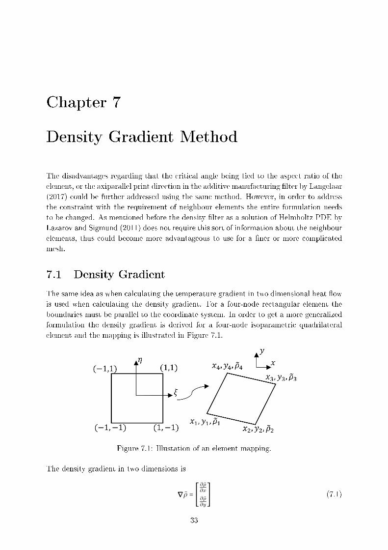
7.1 Density Gradient . . . . . . . . . . . . . . . . . . . . . . . . . . . . . . . . . . 33
7.2 Additive Manufacturing Filter . . . . . . . . . . . . . . . . . . . . . . . . . . 34
7.2.1 Formulation . . . . . . . . . . . . . . . . . . . . . . . . . . . . . . . . . 35
i
Page 10
ii CONTENTS
7.2.2 Sensitivity Analysis . . . . . . . . . . . . . . . . . . . . . . . . . . . . . 36
7.2.3 The Function w(∇∇∇ρ) . . . . . . . . . . . . . . . . . . . . . . . . . . . . 38
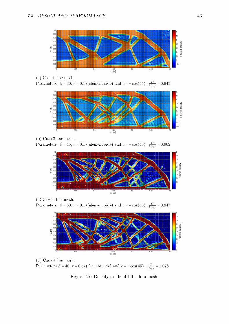
7.3 Result and performance . . . . . . . . . . . . . . . . . . . . . . . . . . . . . . 39
8 Discussion and Further Work 44
Bibliography 46
Page 11
List of Figures
3.1 The eectiv Young's modulus as a function of ρp (Christensen et al., 2008) 11
3.2 Regularized Heaviside step functions. . . . . . . . . . . . . . . . . . . . . . . . 16
4.1 Commonly used materials in additive manufacturing. . . . . . . . . . . . . . 18
4.2 The process scheme for additive manufacturing. . . . . . . . . . . . . . . . . 19
6.1 A fully supported element for the two dimensional case. . . . . . . . . . . . 24
6.2 Baseplates for the additive manufacturing lter. . . . . . . . . . . . . . . . . 27
6.3 Illustration of the geometry and boundary conditions. . . . . . . . . . . . . . 27
6.4 Topology optimization solved using the modied SIMP method and a den-
sity lter. . . . . . . . . . . . . . . . . . . . . . . . . . . . . . . . . . . . . . . . 28
6.5 Additive manufacturing lter by Langelaar (2017) applied on the coarse
mesh. . . . . . . . . . . . . . . . . . . . . . . . . . . . . . . . . . . . . . . . . . . 29
6.6 Additive manufacturing lter by Langelaar (2017) applied on the ne mesh. 30
6.7 Computational time curve for the method by Langelaar (2017). . . . . . . . 31
7.1 Illustation of an element mapping. . . . . . . . . . . . . . . . . . . . . . . . . 33
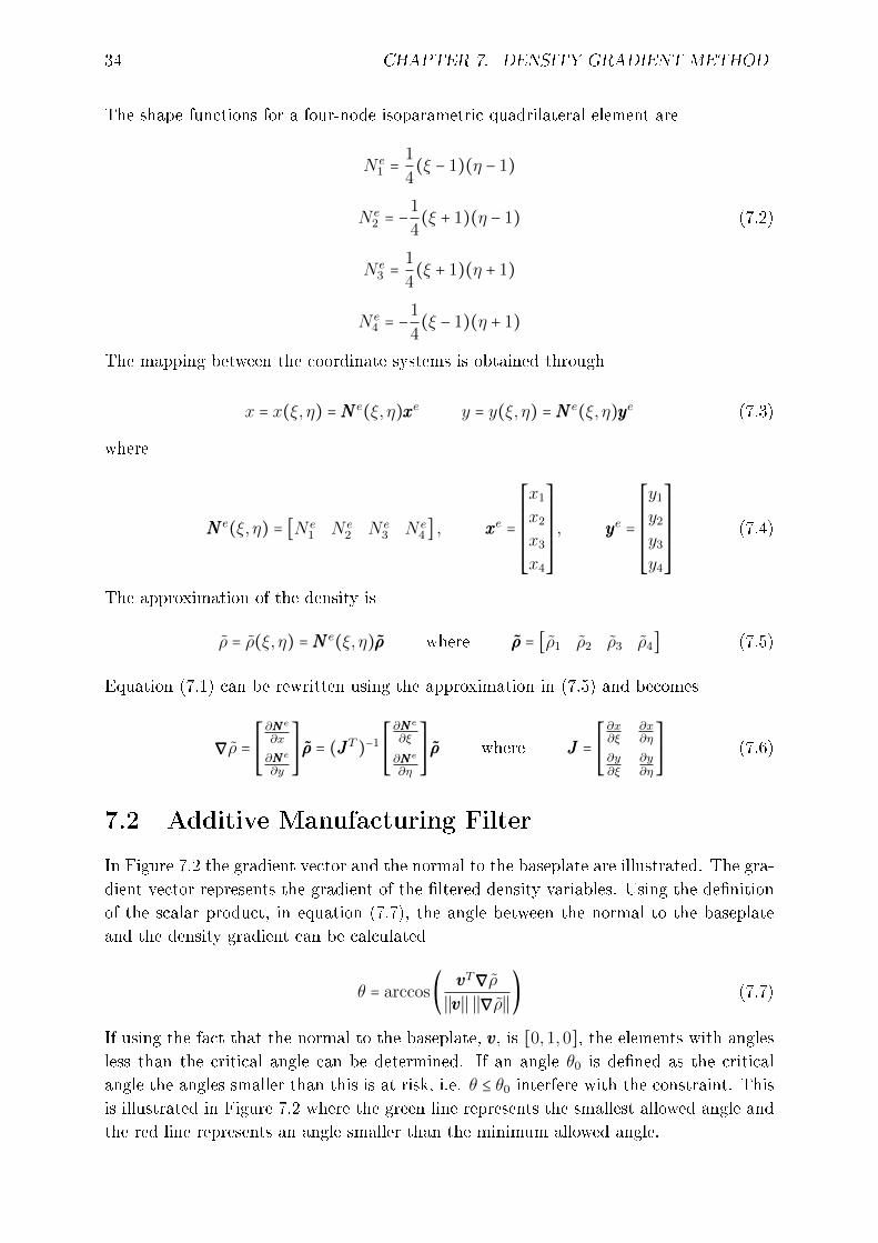
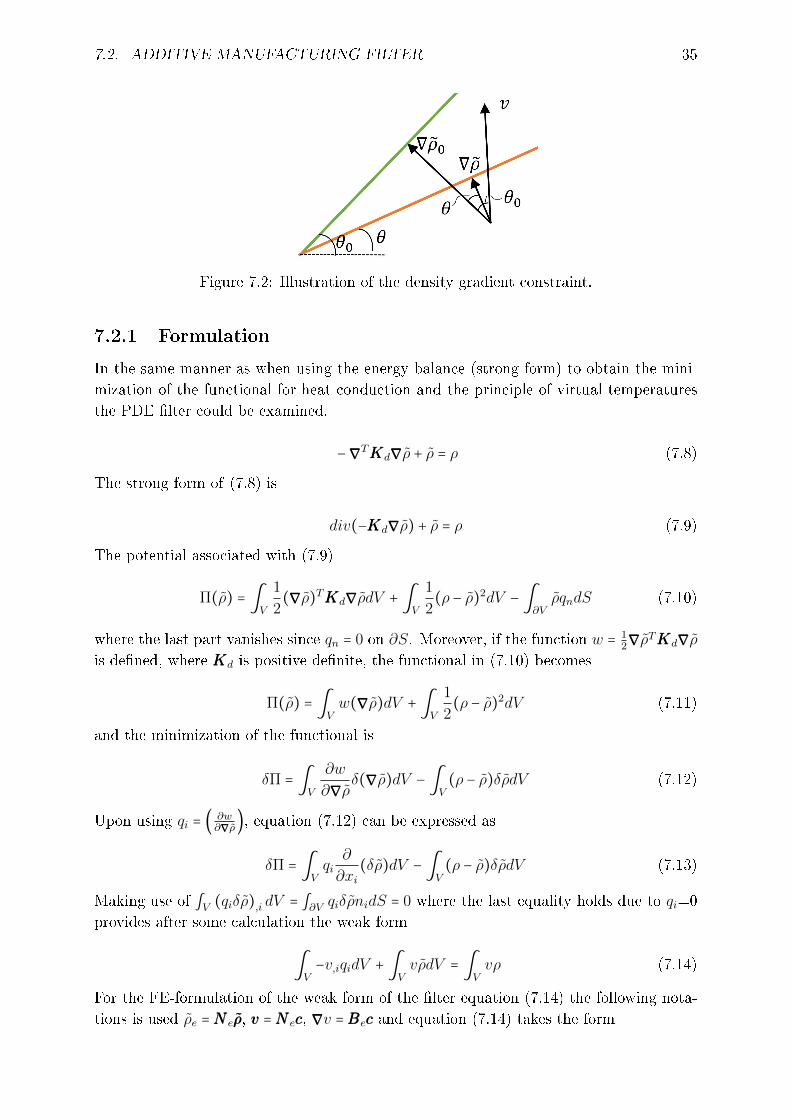
7.2 Illustration of the density gradient constraint. . . . . . . . . . . . . . . . . . 35
7.3 Filter equation w(∇∇∇ρ). . . . . . . . . . . . . . . . . . . . . . . . . . . . . . . . 39
7.4 Illustration of the geometry and boundary conditions. . . . . . . . . . . . . . 39
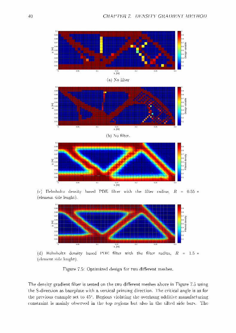
7.5 Optimized design for two dierent meshes. . . . . . . . . . . . . . . . . . . . 40
7.6 Density gradient lter coarse mesh. . . . . . . . . . . . . . . . . . . . . . . . . 42
7.7 Density gradient lter ne mesh. . . . . . . . . . . . . . . . . . . . . . . . . . 43
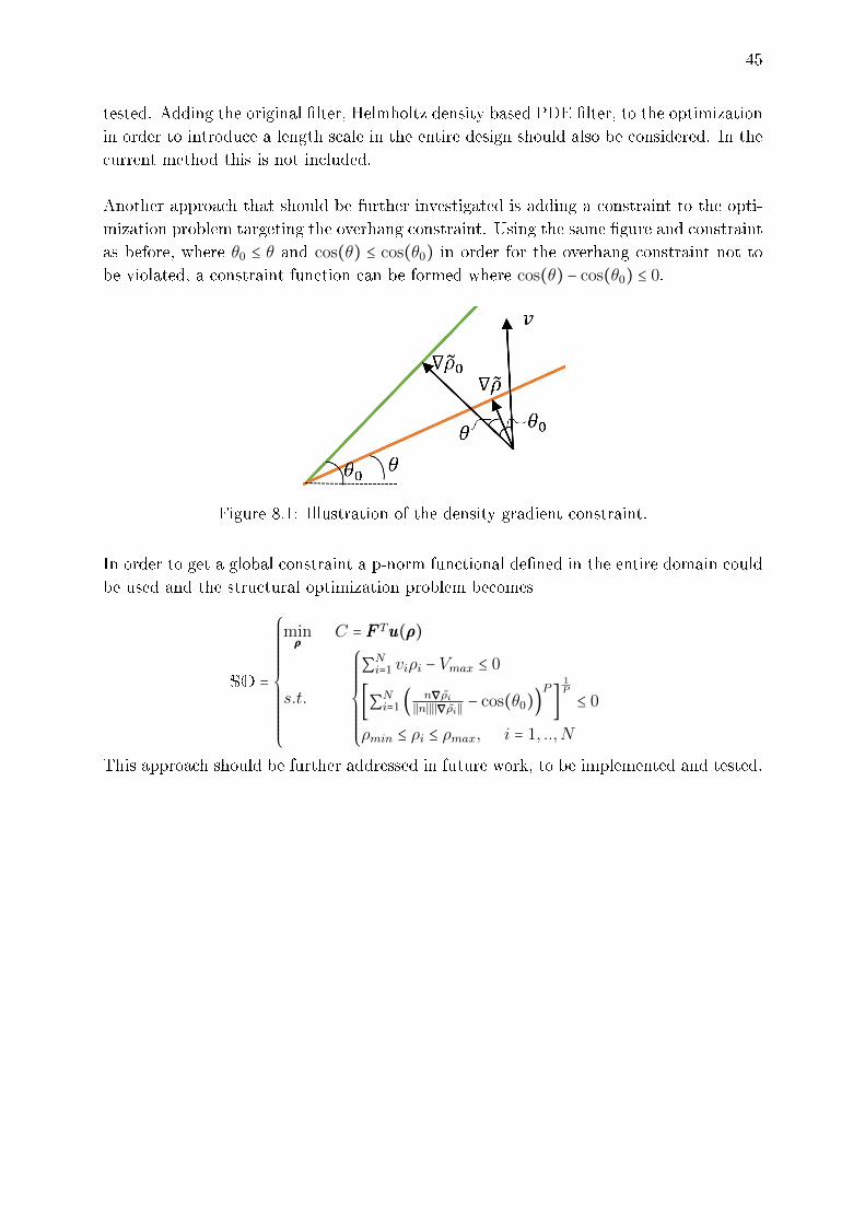
8.1 Illustration of the density gradient constraint. . . . . . . . . . . . . . . . . . 45
iii
Page 12
List of Tables
6.1 Relative compliance for the method by Langelaar (2017) . . . . . . . . . . . 31
iv
Page 14
Chapter 1
Introduction
1.1 Background
In the industry, rapid prototyping, RP, is a term that describes a process that rapidly
creates a system or a part representation, i.e. creating something fast that will result
in a prototype. Additive manufacturing, AM, is a formalized term and was previously
denoted rapid prototyping. Additive manufacturing works by creating the part from eg.
CAD data adding the material in layers, contrary to the more traditional procedure where
material is subtracted. This can be used to shorten the product development times and
cost and can be manufactured using both plastic and a variety of metals (Gibson et al.,
2015).
Structural optimization focus on making an assemblage of materials sustain loads in the
"best" way. The objective could for an example be maximizing the stiness of a struc-
ture. A structural optimization problem consists of an objective function that classies
designs, design variables that describe the design and state variables that represent the
response of a structure. There are dierent types of structural optimization problems and
these are sizing optimization, shape optimization and topology optimization. Topology
optimization optimizes the material layout in the design space allowing design variables to
take the value zero (Christensen et al., 2008). The method is today used in the industry
early in the product development to allow designers to investigate structurally ecient
concepts. It is integrated in some of the leading FEM softwares today such as ANSYS
Mechanical (ANSYS, 2017) and OptiStruct by Altair (OptiStruct, 2017).
The ability of additive manufacturing to manufacture very complex topology, which often
is the outcome from topology optimization, makes topology optimization a good design
tool for additive manufacturing. In order to ensure manufacturability using additive
manufacturing, support material is often necessary to overcome certain constraints such
as overhang, minimum feature size, anisotropy to prevent collapsing during fabrication
(Clausen, 2016).
This work will target the overhang constraint where the goal is to achieve self-supporting
structures without support material. Usually support material is used during manufac-
1
Page 15
2 CHAPTER 1. INTRODUCTION
turing which will increase the print time, the material cost and resources to remove the
support structures. Instead of using support structures one could modify the optimal
topology to not interfere with the overhang constraint. Leary et al., (2014) proposed
a novel method that modies the optimal topology to enable additive manufacturing.
Gaynor and Guest (2016) proposed a method where a combination of local projection to
enforce minimum length scale and support region projection address both the minimum
feature size constraint and the overhang constraint. Langelaar (2017) presents a method
that can be included in conventional density based topology optimization and is imple-
mented with a density lter. The method proposed by Langelaar (2017) comes with many
advantages such as time eciency and the production of self supporting structures. How-
ever, in this approach the self-supporting angle is tied to the aspect ratio of the elements
and the method requires information about neighbouring elements which for ne meshes
or complex domains and geometries become an expensive operation.
The density lter as a solution of Helmholtz PDE by Lazarov and Sigmund (2011) does
not require information about the neighbouring elements, thus could become more ad-
vantageous to use for ner or more complicated meshes. Another advantageous property
with Helmholtz PDE lter is that the method provides nodal values of the ltered de-
sign variable. Using the nodal values it becomes simple to calculate the density gradient
which in turn could provide an angle between the element gradient and another vector,
for example the baseplate vector.
1.2 Aim
The aim of this master thesis is to further examine the method proposed by Langelaar
(2017) and to examine the possibility to extend the Helmholtz PDE lter to include the
density gradients in the formulation such that a self supporting structure is obtained.
Isotropic and linear elastic material will be considered throughout the report and the
optimization problem will be solved using the optimality criteria with a density lter for
the method proposed by Langelaar (2017). The additive manufacturing lter is provided
by Langelaar (2017) and is implemented in MATLAB. The proposed method will be
solved using the method of moving asymptotes by Svanberg (1987) with an augmented
Helmholtz PDE lter and is implemented in MATLAB and Fortran.
1.3 Structure of Report
The rst chapters in the thesis will provide the necessary theory needed for the research.
Chapter 2 will derive the nite element formulation. Chapter 3 will provide the necessary
information in order to solve the optimization problem. Beginning with the general infor-
mation regarding structural optimization with focus on topology optimization continuing
with solution strategies for the topology optimization problem and ltering techniques. In
Chapter 4 the concept of additive manufacturing will be presented. For readers familiar
with these subjects it is recommended to move on to Chapter 5. In Chapter 5 state-of-the
Page 16
1.3. STRUCTURE OF REPORT 3
art methods regarding constraints for additive manufacturing in topology optimization
are presented. In Chapter 6 the method proposed by Langelaar (2017) is examined by
presenting the theory regarding the method, testing the method and discussing the result.
Chapter 7 proposes a method using an altered Helmholtz PDE lter. The chapter will
start by formulating the problem, the topology optimization and ltering. The chapter
continues with integrating the overhang constraint into the Helmholtz-type PDE lter
and presenting the result. The nal chapter, Chapter 8, will discuss the obtained result
and further work.
Page 17
Chapter 2
Finite Element Method
The nite element formulation follows the derivation according to Saabye Ottosen and
Ristinmaa (2005). The nite element formulation is based on the weak form which is
derived from the equation of balance of linear momentum
∫VρuidV = ∫
VtidS + ∫
Vbidv (2.1)
where ρ = ρ(xi, t) is the mass density, ui = u(xi, t) is the acceleration eld, ti = ti(xi, t)
is the traction vector and bi = bi(xi, t) is the body force vector. Using the divergence
theorem and that the relation hold for any volume provides the strong form of equation
of motion
σij,j + bi = ρui (2.2)
To obtain the weak form equation (2.2) is expressed as
∫V[(σijvi),j − σijvi,j]dV + ∫
V[vibi − ρviui]dV = 0 (2.3)
Using the divergence theorem and the fact that vi is an arbitrary vector not related to ui,
and dening εvij =12(vi,j + vj,i) where εvij is related to the weight function vi in the same
manner as εij is related to the displacement ui as well as symmetry of the stress tensor
σij provides
∫VρviuidV + ∫
Vvi,jσijdV = ∫
SvitidS + ∫
VvibidV (2.4)
Exploring the symmetry of σij yields
vi,jσij = εvijσij (2.5)
which enables (2.4) to be formulated as the principle of virtual work
∫VρviuidV + ∫
VεvijσijdV = ∫
SvitidS + ∫
VvibidV (2.6)
Rewriting this to voigt form provides the following expression
∫VρvvvT uuudV + ∫
V(εεεv)TσσσdV = ∫
SvvvTtttdS + ∫
VvvvTbbbdV (2.7)
4
Page 18
5
To be able to express the displacement as an approximation through the entire body
using the nite element method, some notations needs to be established. uuu = uuu(xi, t) is
the displacement vector, NNN = NNN(xi) is the global shape function, aaa = aaa(t) is the nodal
displacement, vvv is the weight function according to the Galerkin method. From this it
follows
uuu =NNNaaa BBB =BBB(xi) =∂NNN
∂xiεεε =BBBaaa vvv =NNNccc (2.8)
The notations in (2.8) put into (2.7) and stating that ccc is arbitrary provides the notation
for the nite element method. Assuming static conditions uuu = 000 will result in that the
equation of motion is reduced to the equilibrium conditions and becomes
∫VBBBTσσσdV = ∫
SNNNTtttdS + ∫
VNNNTbbbdV (2.9)
For a linear elastic material the stress tensor can be approximated as σσσ =DDDεεε =DDDBBBaaa where
DDD is the constitutive matrix. For isotropic materials the constitutive matrix DDD becomes
DDD =E
(1 + v)(1 − 2v)
⎡⎢⎢⎢⎢⎢⎢⎢⎢⎢⎢⎢⎢⎢⎣
1 − v v v 0 0 0
v 1 − v v 0 0 0
v v 1 − v 0 0 0
0 0 0 12(1 − 2v) 0 0
0 0 0 0 12(1 − 2v) 0
0 0 0 0 0 12(1 − 2v)
⎤⎥⎥⎥⎥⎥⎥⎥⎥⎥⎥⎥⎥⎥⎦
(2.10)
where E is the modulus of elasticity and v is Poisson's ratio. Inserting (2.9) into (2.10)
result in
(∫VBBBTDDDBBBdV )aaa = ∫
SNNNTtttdS + ∫
VNNNbbbdV (2.11)
To simplify the method, the stiness matrix KKK, the load vector fff are dened as
KKK = ∫VBBBTDDDBBBdV fff = ∫
SNNNTtttdS + ∫
VNNNbbbdV (2.12)
Combining (2.11) and (2.12) provide
KKKaaa = fff (2.13)
Page 19
Chapter 3
Optimization
3.1 Structural Optimization
Structural optimization means making a structure sustain loads in the best way. The
general mathematical form of a structural optimization problem is usually written as
(SO)
⎧⎪⎪⎪⎪⎪⎪⎪⎪⎨⎪⎪⎪⎪⎪⎪⎪⎪⎩
minimize g0(xxx,yyy) with respect to xxx and yyy
subject to
⎧⎪⎪⎪⎪⎪⎨⎪⎪⎪⎪⎪⎩
behaviorial constraints on yyy
design constraints on xxx
equilibrium constraint
(3.1)
where g0 is the objective function which is usually chosen as a minimization problem, i.e.
choose g0 such that a small value is better than a large. The variable that describes the
design is the design variable, xxx, which can be changed during the optimization. The last
variable, yyy, is called the state variable and represents the response of the structure. There
are several types of structural optimization problems: rst sizing optimization where the
design variable represents a kind of structural thickness, shape optimization where the
design variable represents the form or contour of a boundary, and topology optimization.
Topology optimization provides an answer to "How to place the material within a pre-
scribed design domain in order to obtain the best structural performance?". It was rst
introduced in a seminal paper by Bendsøe and Kikuchi (1988) where a homogenization
method produced an optimal shape as well as topology of a mechanical element. Since
its introduction, topology optimization has undergone a huge development in various di-
rections such as density approach, phase eld approach and several others.
The formulation in (3.1) is usually referred to as simultaneous formulation since the equi-
librium equation is solved simultaneously with the the optimization. If the state variable
is uniquely dened for a given design variable, e.g. ifKKK(xxx) is invertible for all xxx such that
uuu = uuu(xxx) =KKK(xxx)−1FFF , the equilibrium equation can be eliminated from equation (3.1) by
treating uuu(xxx) as a given function and equation (3.1) instead becomes (Christensen et al.,
2008)
6
Page 20
3.1. STRUCTURAL OPTIMIZATION 7
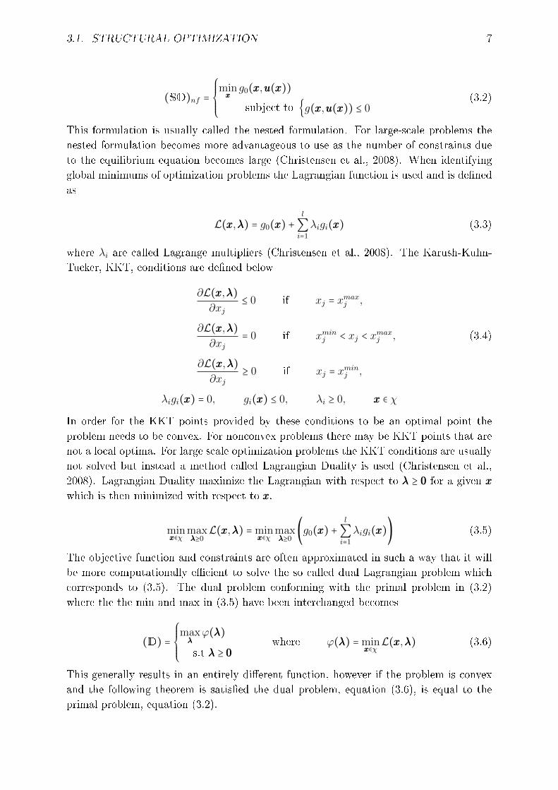
(SO)nf =
⎧⎪⎪⎪⎨⎪⎪⎪⎩
minxxxg0(xxx,uuu(xxx))
subject to g(xxx,uuu(xxx)) ≤ 0(3.2)
This formulation is usually called the nested formulation. For large-scale problems the
nested formulation becomes more advantageous to use as the number of constraints due
to the equilibrium equation becomes large (Christensen et al., 2008). When identifying
global minimums of optimization problems the Lagrangian function is used and is dened
as
L(xxx,λλλ) = g0(xxx) +l
∑i=1
λigi(xxx) (3.3)
where λi are called Lagrange multipliers (Christensen et al., 2008). The Karush-Kuhn-
Tucker, KKT, conditions are dened below
∂L(xxx,λλλ)
∂xj≤ 0 if xj = x
maxj ,
∂L(xxx,λλλ)
∂xj= 0 if xminj < xj < x
maxj , (3.4)
∂L(xxx,λλλ)
∂xj≥ 0 if xj = x
minj ,
λigi(xxx) = 0, gi(xxx) ≤ 0, λi ≥ 0, xxx ∈ χ
In order for the KKT points provided by these conditions to be an optimal point the
problem needs to be convex. For nonconvex problems there may be KKT points that are
not a local optima. For large scale optimization problems the KKT conditions are usually
not solved but instead a method called Lagrangian Duality is used (Christensen et al.,
2008). Lagrangian Duality maximize the Lagrangian with respect to λλλ ≥ 000 for a given xxx
which is then minimized with respect to xxx.
minxxx∈χ max
λλλ≥0L(xxx,λλλ) = min
xxx∈χ maxλλλ≥0
(g0(xxx) +l
∑i=1
λigi(xxx)) (3.5)
The objective function and constraints are often approximated in such a way that it will
be more computationally ecient to solve the so called dual Lagrangian problem which
corresponds to (3.5). The dual problem conforming with the primal problem in (3.2)
where the the min and max in (3.5) have been interchanged becomes
(D) =
⎧⎪⎪⎪⎨⎪⎪⎪⎩
maxλλλ
ϕ(λλλ)
s.t λλλ ≥ 000where ϕ(λλλ) = min
xxx∈χ L(xxx,λλλ) (3.6)
This generally results in an entirely dierent function, however if the problem is convex
and the following theorem is satised the dual problem, equation (3.6), is equal to the
primal problem, equation (3.2).
Page 21
8 CHAPTER 3. OPTIMIZATION
Let the problem be convex and satisfy Slater's constraint qualication (CQ), i.e. there
exists a point xxx ∈ χ such that gi(xxx) < 0, i = 1, ...l. Let x∗ be a local (i.e. also global)
minimum of the problem. Then there exists a λλλ∗ such that (xxx∗,λλλ∗) is a KKT point of the
problem. (Christensen et al., 2008)
The dual objective function, ϕ, is always concave which means that it is easy to maximize.
If minxxx∈χ L(xxx,λλλ) has one solution for a given λλλ then ϕ is dierentiable at λλλ and can be solved
through
∂ϕ(λλλ)
∂λi= gi(xxx
∗(λλλ)) i = 1, ..l where xxx∗(λλλ) = minxxx∈χ L(xxx,λλλ) (3.7)
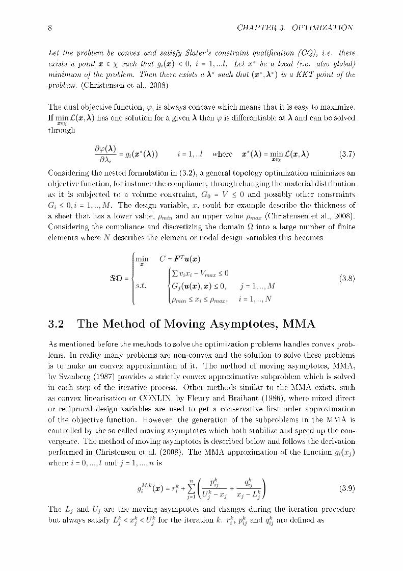
Considering the nested formulation in (3.2), a general topology optimization minimizes an
objective function, for instance the compliance, through changing the material distribution
as it is subjected to a volume constraint, G0 = V ≤ 0 and possibly other constraints
Gi ≤ 0, i = 1, ..,M . The design variable, x, could for example describe the thickness of
a sheet that has a lower value, ρmin and an upper value ρmax (Christensen et al., 2008).
Considering the compliance and discretizing the domain Ω into a large number of nite
elements where N describes the element or nodal design variables this becomes
SO =
⎧⎪⎪⎪⎪⎪⎪⎪⎪⎪⎨⎪⎪⎪⎪⎪⎪⎪⎪⎪⎩
minxxx
C = FFF Tuuu(xxx)
s.t.
⎧⎪⎪⎪⎪⎪⎨⎪⎪⎪⎪⎪⎩
∑ vixi − Vmax ≤ 0
Gj(uuu(xxx),xxx) ≤ 0, j = 1, ..,M
ρmin ≤ xi ≤ ρmax, i = 1, ..,N
(3.8)
3.2 The Method of Moving Asymptotes, MMA
As mentioned before the methods to solve the optimization problems handles convex prob-
lems. In reality many problems are non-convex and the solution to solve these problems
is to make an convex approximation of it. The method of moving asymptotes, MMA,
by Svanberg (1987) provides a strictly convex approximative subproblem which is solved
in each step of the iterative process. Other methods similar to the MMA exists, such
as convex linearisation or CONLIN, by Fleury and Braibant (1986), where mixed direct
or reciprocal design variables are used to get a conservative rst order approximation
of the objective function. However, the generation of the subproblems in the MMA is
controlled by the so called moving asymptotes which both stabilize and speed up the con-
vergence. The method of moving asymptotes is described below and follows the derivation
performed in Christensen et al. (2008). The MMA approximation of the function gi(xj)
where i = 0, ..., l and j = 1, ..., n is
gM,ki (xxx) = rki +
n
∑j=1
(pkij
Ukj − xj
+qkij
xj −Lkj) (3.9)
The Lj and Uj are the moving asymptotes and changes during the iteration procedure
but always satisfy Lkj < xkj < U
kj for the iteration k. rki , p
kij and q
kij are dened as
Page 22
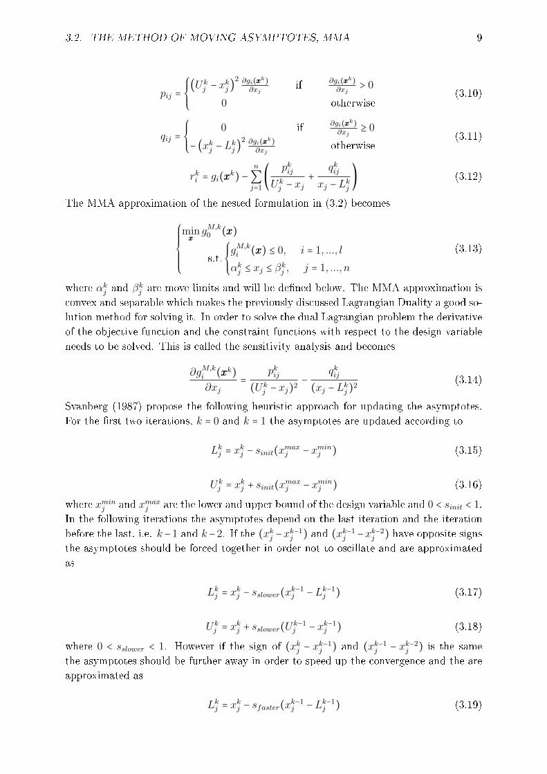
3.2. THE METHOD OF MOVING ASYMPTOTES, MMA 9
pij =
⎧⎪⎪⎨⎪⎪⎩
(Ukj − x
kj )
2 ∂gi(xxxk)∂xj
if ∂gi(xxxk)∂xj
> 0
0 otherwise(3.10)
qij =
⎧⎪⎪⎨⎪⎪⎩
0 if ∂gi(xxxk)∂xj
≥ 0
− (xkj −Lkj )
2 ∂gi(xxxk)∂xj
otherwise(3.11)
rki = gi(xxxk) −
n
∑j=1
(pkij
Ukj − xj
+qkij
xj −Lkj) (3.12)
The MMA approximation of the nested formulation in (3.2) becomes
⎧⎪⎪⎪⎪⎪⎨⎪⎪⎪⎪⎪⎩
minxxxgM,k
0 (xxx)
s.t.
⎧⎪⎪⎨⎪⎪⎩
gM,ki (xxx) ≤ 0, i = 1, ..., l
αkj ≤ xj ≤ βkj , j = 1, ..., n
(3.13)
where αkj and βkj are move limits and will be dened below. The MMA approximation is
convex and separable which makes the previously discussed Lagrangian Duality a good so-
lution method for solving it. In order to solve the dual Lagrangian problem the derivative
of the objective function and the constraint functions with respect to the design variable
needs to be solved. This is called the sensitivity analysis and becomes
∂gM,ki (xxxk)
∂xj=
pkij(Uk
j − xj)2−
qkij(xj −Lkj )
2(3.14)
Svanberg (1987) propose the following heuristic approach for updating the asymptotes.
For the rst two iterations, k = 0 and k = 1 the asymptotes are updated according to
Lkj = xkj − sinit(x
maxj − xminj ) (3.15)
Ukj = x
kj + sinit(x
maxj − xminj ) (3.16)
where xminj and xmaxj are the lower and upper bound of the design variable and 0 < sinit < 1.
In the following iterations the asymptotes depend on the last iteration and the iteration
before the last, i.e. k−1 and k−2. If the (xkj −xk−1j ) and (xk−1
j −xk−2j ) have opposite signs
the asymptotes should be forced together in order not to oscillate and are approximated
as
Lkj = xkj − sslower(x
k−1j −Lk−1
j ) (3.17)
Ukj = x
kj + sslower(U
k−1j − xk−1
j ) (3.18)
where 0 < sslower < 1. However if the sign of (xkj − xk−1j ) and (xk−1
j − xk−2j ) is the same
the asymptotes should be further away in order to speed up the convergence and the are
approximated as
Lkj = xkj − sfaster(x
k−1j −Lk−1
j ) (3.19)
Page 23
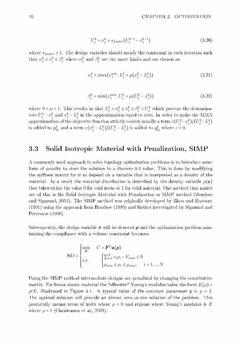
10 CHAPTER 3. OPTIMIZATION
Ukj = x
kj + sfaster(U
k−1j − xk−1
j ) (3.20)
where sfaster > 1. The design variables should satisfy the constraint in each iteration such
that αkj ≤ xkj ≤ β
kj where αkj and β
kj are the move limits and are chosen as
αkj = max(xminj , Lkj + µ(x
kj −L
kj )) (3.21)
βkj = min(xmaxj , Uk
j + µ(Ukj − x
kj )) (3.22)
where 0 < µ < 1. This results in that Lkj < αkj ≤ x
kj ≤ β
kj < U
kj which prevent the denomina-
tors Ukj − x
kj and x
kj −L
kj in the approximation equal to zero. In order to make the MMA
approximation of the objective function strictly convex usually a term ε(Ukj −x
kj )/(U
kj −L
kj )
is added to pk0j and a term ε(xkj −Lkj )/(U
kj −L
kj ) is added to qk0j where ε > 0.
3.3 Solid Isotropic Material with Penalization, SIMP
A commonly used approach to solve topology optimization problems is to introduce some
form of penalty to steer the solution to a discrete 0-1 value. This is done by modifying
the stiness matrix for it to depend on a variable that is interpreted as a density of the
material. As a result the material distribution is described by the density variable ρ(xxx)
that takes either the value 0 for void areas or 1 for solid material. One method that makes
use of this is the Solid Isotropic Material with Penalization or SIMP method (Bendsøe
and Sigmund, 2004). The SIMP method was originally developed by Zhou and Rozvany
(1991) using the approach from Bendsøe (1989) and further investigated by Sigmund and
Petersson (1998).
Subsequently, the design variable xxx will be denoted ρρρ and the optimization problem min-
imizing the compliance with a volume constraint becomes
SO =
⎧⎪⎪⎪⎪⎪⎪⎨⎪⎪⎪⎪⎪⎪⎩
minρρρ
C = FFF Tuuu(ρρρ)
s.t.
⎧⎪⎪⎨⎪⎪⎩
∑Ni=1 viρi − Vmax ≤ 0
ρmin ≤ ρi ≤ ρmax, i = 1, ..,N
Using the SIMP method intermediate designs are penalized by changing the constitutive
matrix. For linear elastic material the "eective" Young's modulus takes the form E(ρ) =
ρpE, illustrated in Figure 3.1. A typical value of the constant parameter p is p = 3.
The optimal solution will provide an almost zero to one solution of the problem. This
practically means areas of holes where ρ = 0 and regions where Young's modulus is E
where ρ = 1 (Christensen et al., 2008).
Page 24
3.3. SOLID ISOTROPIC MATERIAL WITH PENALIZATION, SIMP 11
Figure 3.1: The eectiv Young's modulus as a function of ρp (Christensen et al., 2008)
In the classical SIMP approach described above the elements with no stiness is taken
into account by the fact that the lower limit, ρmin, imposes a value slightly larger than
zero. Instead of this consideration, the modied SIMP approach could be used. Young's
modulus instead takes the form
Ee(ρe) = Emin + ρpe(E0 −Emin) ρe ∈ [0,1] (3.23)
The extra variable Emin is the stiness of the void material, still dierent from zero to
avoid singularity of the stiness matrix. The modied SIMP compared with the classical
SIMP comes with a number of benets, such as covering two-phase design problems and
providing a straightforward implementation of additional lters (Sigmund, 2007).
3.3.1 The optimality criteria method, OC, using SIMP
The topology optimization problem could be solved using the MMA approximation but
also with the optimality criteria method, or OC method. The OC method is described
below and follows the derivation performed in Christensen et al. (2008). The OC method is
based on a truncated Taylor approximation of the objective function, here the compliance,
which can be expressed as
C(ρρρ) ≈ C(ρρρk) +n
∑e=1
∂C
∂ye∣ρρρ=ρρρk
(ye − yke ) (3.24)
The intervening variable for the optimality criteria method is ye = ρ−αe where α > 0. Using
this, the derivative of the compliance becomes
∂C(ρρρ)
∂ρe= −(uuuke)
T ∂KKKM
∂ρρρuuu0e at ρρρ = ρρρk (3.25)
where uuu(ρρρk) = KKKM(ρρρk)−1FFF . Using the SIMP approach, the global stiness matrix is
calculated using the eective Young's modulus. Evaluation of ∂C∂ye
with (3.24) and (3.25)
provides the subproblem:
SO =
⎧⎪⎪⎪⎪⎪⎪⎨⎪⎪⎪⎪⎪⎪⎩
minρρρ
n
∑e=1
(ρke)1+αα ((uuuke)
Tp(ρke)p−1 ∂KKKM
∂ρρρ uuuke)ρ
−αe
s.t
⎧⎪⎪⎨⎪⎪⎩
ρρρTaaa = V
ρmin ≤ ρe ≤ ρmax, e = 1, ..., n
(3.26)
Page 25
12 CHAPTER 3. OPTIMIZATION
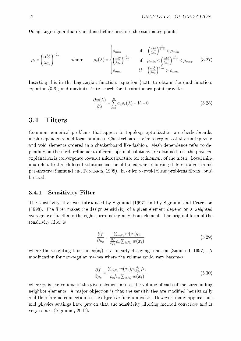
Using Lagrangian duality as done before provides the stationary points.
ρe = (αbkeλae
)
11+α
where ρe(λ) =
⎧⎪⎪⎪⎪⎪⎪⎪⎪⎨⎪⎪⎪⎪⎪⎪⎪⎪⎩
ρmin if (αbkeλae
)
11+α
< ρmin
(αbkeλae
)
11+α
if ρmin ≤ (αbkeλae
)
11+α
≤ ρmax
ρmax if (αbkeλae
)
11+α
> ρmax
(3.27)
Inserting this in the Lagrangian function, equation (3.3), to obtain the dual function,
equation (3.6), and maximize it to search for it's stationary point provides
∂ϕ(λ)
∂λ=
n
∑e=1
aeρe(λ) − V = 0 (3.28)
3.4 Filters
Common numerical problems that appear in topology optimization are checkerboards,
mesh dependency and local minimas. Checkerboards refer to regions of alternating solid
and void elements ordered in a checkerboard like fashion. Mesh dependence refer to de-
pending on the mesh renement dierent optimal solutions are obtained, i.e. the physical
explanation is convergence towards microstructure for renement of the mesh. Local min-
ima refers to that dierent solutions can be obtained when choosing dierent algorithmic
parameters (Sigmund and Petersson, 1998). In order to avoid these problems lters could
be used.
3.4.1 Sensitivity Filter
The sensitivity lter was introduced by Sigmund (1997) and by Sigmund and Petersson
(1998). The lter makes the design sensitivity of a given element depend on a weighted
average over itself and the eight surrounding neighbour element. The original form of the
sensitivity lter is
∂f
∂ρe=∑i∈Ne w(xxxi)ρi
∂f∂ρiρe∑i∈Ne w(xxxi)
(3.29)
where the weighting function w(xxxi) is a linearly decaying function (Sigmund, 1997). A
modication for non-regular meshes where the volume could vary becomes
∂f
∂ρe=∑i∈Ne w(xxxi)ρi
∂f∂ρi
/vi
ρe/ve∑i∈Ne w(xxxi)(3.30)
where ve is the volume of the given element and vi the volume of each of the surrounding
neighbor elements. A major objection is that the sensitivities are modied heuristically
and therefore no connection to the objective function exists. However, many applications
and physics settings have proven that the sensitivity ltering method converges and is
very robust (Sigmund, 2007).
Page 26
3.4. FILTERS 13
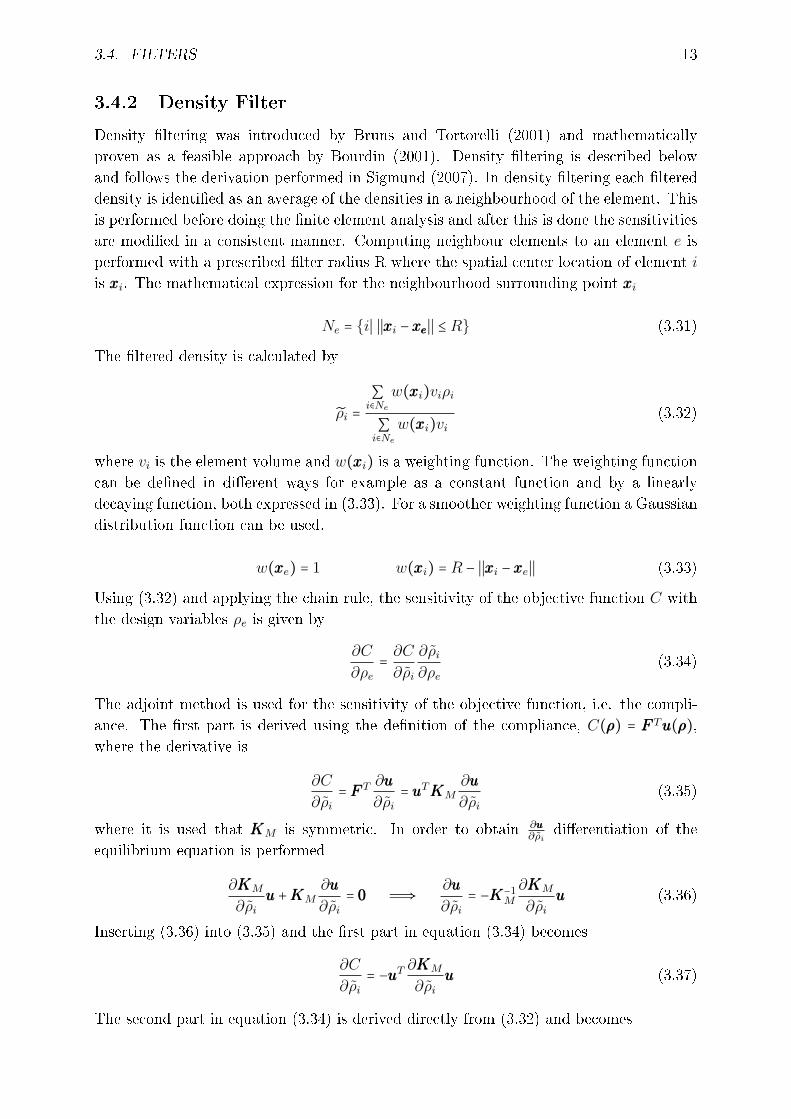
3.4.2 Density Filter
Density ltering was introduced by Bruns and Tortorelli (2001) and mathematically
proven as a feasible approach by Bourdin (2001). Density ltering is described below
and follows the derivation performed in Sigmund (2007). In density ltering each ltered
density is identied as an average of the densities in a neighbourhood of the element. This
is performed before doing the nite element analysis and after this is done the sensitivities
are modied in a consistent manner. Computing neighbour elements to an element e is
performed with a prescribed lter radius R where the spatial center location of element i
is xxxi. The mathematical expression for the neighbourhood surrounding point xxxi
Ne = i∣ ∣∣xxxi −xexexe∣∣ ≤ R (3.31)
The ltered density is calculated by
ρi =
∑i∈Ne
w(xxxi)viρi
∑i∈Ne
w(xxxi)vi(3.32)
where vi is the element volume and w(xxxi) is a weighting function. The weighting function
can be dened in dierent ways for example as a constant function and by a linearly
decaying function, both expressed in (3.33). For a smoother weighting function a Gaussian
distribution function can be used.
w(xxxe) = 1 w(xxxi) = R − ∣∣xxxi −xxxe∣∣ (3.33)
Using (3.32) and applying the chain rule, the sensitivity of the objective function C with
the design variables ρe is given by
∂C
∂ρe=∂C
∂ρi
∂ρi∂ρe
(3.34)
The adjoint method is used for the sensitivity of the objective function, i.e. the compli-
ance. The rst part is derived using the denition of the compliance, C(ρρρ) = FFF Tuuu(ρρρ),
where the derivative is
∂C
∂ρi= FFF T ∂uuu
∂ρi= uuuTKKKM
∂uuu
∂ρi(3.35)
where it is used that KKKM is symmetric. In order to obtain ∂uuu∂ρi
dierentiation of the
equilibrium equation is performed
∂KKKM
∂ρiuuu +KKKM
∂uuu
∂ρi= 000 Ô⇒
∂uuu
∂ρi= −KKK−1
M
∂KKKM
∂ρiuuu (3.36)
Inserting (3.36) into (3.35) and the rst part in equation (3.34) becomes
∂C
∂ρi= −uuuT
∂KKKM
∂ρiuuu (3.37)
The second part in equation (3.34) is derived directly from (3.32) and becomes
Page 27
14 CHAPTER 3. OPTIMIZATION
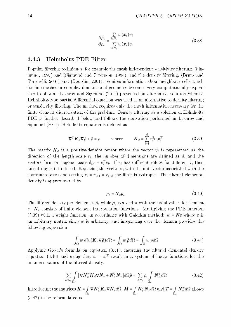
∂ρi∂ρe
=
∑i∈Ne
w(xxxi)vi
∑i∈Ne
w(xxxi)vi(3.38)
3.4.3 Helmholtz PDE Filter
Popular ltering techniques, for example the mesh independent sensitivity ltering, (Sig-
mund, 1997) and (Sigmund and Petersson, 1998), and the density ltering, (Bruns and
Tortorelli, 2001) and (Bourdin, 2001), requires information about neighbour cells which
for ne meshes or complex domains and geometry becomes very computationally expen-
sive to obtain. Lazarov and Sigmund (2011) presented an alternative solution where a
Helmholtz-type partial dierential equation was used as an alternative to density ltering
or sensitivity ltering. The method requires only the mesh information necessary for the
nite element discretization of the problem. Density ltering as a solution of Helmholtz
PDE is further described below and follows the derivation performed in Lazarov and
Sigmund (2011). Helmholtz equation is dened as
∇∇∇TKKKd∇∇∇ρ + ρ = ρ where KKKd =d
∑i=1
r2i vvvivvv
Ti (3.39)
The matrix KKKd is a positive-denite tensor where the vector vvvi is represented as the
direction of the length scale ri, the number of dimensions are dened as d, and the
vectors form orthogonal basis δi,j = vTi vi. If ri has dierent values for dierent i, then
anisotropy is introduced. Replacing the vector vvvi with the unit vector associated with the
coordinate axes and setting ri = ri+1 = ri+d the lter is isotropic. The ltered elemental
density is approximated by
ρe =NNN eρρρe (3.40)
The ltered density per element is ρe while ρρρe is a vector with the nodal values for element
e. NNN e consists of nite element interpolation functions. Multiplying the PDE function
(3.39) with a weight function, in accordance with Galerkin method: w = NNNccc where ccc is
an arbitrary matrix since w is arbitrary, and integrating over the domain provides the
following expression
∫Ωw div(KKKd∇∇∇ρρρ)dΩ + ∫
Ωw ρρρdΩ = ∫
Ωw ρdΩ (3.41)
Applying Green's formula on equation (3.41), inserting the ltered elemental density
equation (3.40) and using that w = wT result in a system of linear functions for the
unknown values of the ltered density.
∑i∈Ne∫Ωi
[∇∇∇NNNTeKKKd∇∇∇NNN e +NNN
TeNNN e]dΩρρρ = ∑
i∈Neρi∫
Ωe
NNNTe dΩ (3.42)
Introducing the matricesKKK = ∫Ωi
∇∇∇NNNTeKKKd∇∇∇NNN edΩ,MMM = ∫
Ωi
NNNTeNNN edΩ and TTT = ∫
Ωe
NNNTe dΩ allows
(3.42) to be reformulated as
Page 28
3.5. THRESHOLDING 15
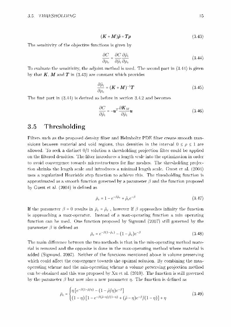
(KKK +MMM)ρρρ = TTTρρρ (3.43)
The sensitivity of the objective functions is given by
∂C
∂ρe=∂C
∂ρi
∂ρi∂ρe
(3.44)
To evaluate the sensitivity, the adjoint method is used. The second part in (3.44) is given
by that KKK, MMM and TTT in (3.43) are constant which provides
∂ρi∂ρe
= (KKK +MMM)−1TTT (3.45)
The rst part in (3.44) is derived as before in section 3.4.2 and becomes
∂C
∂ρi= −uuuT
∂KKKM
∂ρiuuu (3.46)
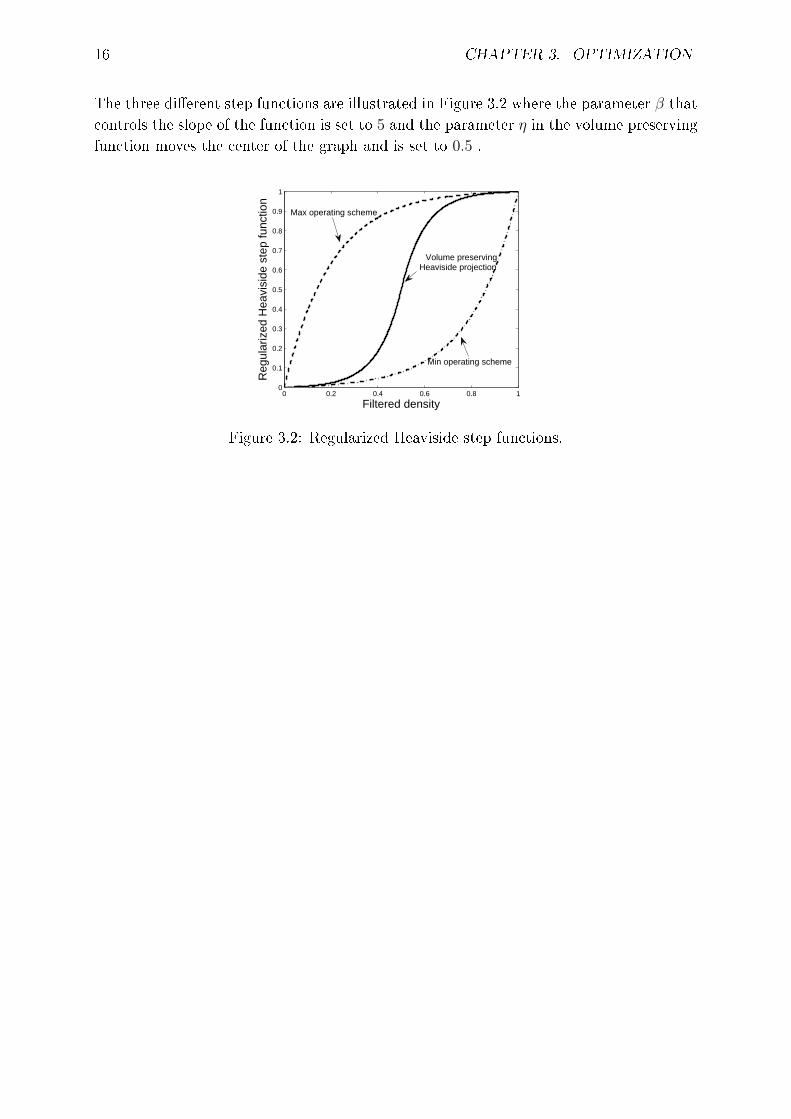
3.5 Thresholding
Filters such as the proposed density lter and Helmholtz PDE lter create smooth tran-
sitions between material and void regions, thus densities in the interval 0 ≤ ρ ≤ 1 are
allowed. To seek a distinct 0/1 solution a thresholding projection lter could be applied
on the ltered densities. The lter introduces a length scale into the optimization in order
to avoid convergence towards microstructures for ne meshes. The thresholding projec-
tion shrinks the length scale and introduces a minimal length scale. Guest et al. (2004)
uses a regularized Heaviside step function to achieve this. The thresholding function is
approximated as a smooth function governed by a parameter β and the function proposed
by Guest et al. (2004) is dened as
ρe = 1 − e−βρe + ρee−β (3.47)
If the parameter β = 0 results in ρe = ρe , however if β approaches innity the function
is approaching a max-operator. Instead of a max-operating function a min operating
function can be used. One function proposed by Sigmund (2007) still governed by the
parameter β is dened as
ρe = e−β(1−ρe) − (1 − ρe)e
−β (3.48)
The main dierence between the two methods is that in the min-operating method mate-
rial is removed and the opposite is done in the max-operating method where material is
added (Sigmund, 2007). Neither of the functions mentioned above is volume preserving
which could aect the convergence towards the optimal solution. By combining the max-
operating scheme and the min-operating scheme a volume preserving projection method
can be obtained and this was proposed by Xu et al. (2010). The function is still governed
by the parameter β but now also a new parameter η. The function is dened as
ρe =
⎧⎪⎪⎨⎪⎪⎩
η [e−β(1−ρ/η) − (1 − ρ/η)e−β]
(1 − η) [1 − e−β(ρ−η)/(1−η) + (ρ − η)e−β/(1 − η)] + η(3.49)
Page 29
16 CHAPTER 3. OPTIMIZATION
The three dierent step functions are illustrated in Figure 3.2 where the parameter β that
controls the slope of the function is set to 5 and the parameter η in the volume preserving
function moves the center of the graph and is set to 0.5 .
0 0.2 0.4 0.6 0.8 10
0.1
0.2
0.3
0.4
0.5
0.6
0.7
0.8
0.9
1
Filtered density
Reg
ular
ized
Hea
visi
de s
tep
func
tion
Volume preserving Heaviside projection
Min operating scheme
Max operating scheme
Figure 3.2: Regularized Heaviside step functions.
Page 30
Chapter 4
Additive Manufacturing
4.1 Rapid Prototyping to Additive Manufacturing
In the industry, rapid prototyping, RP, is a term that describes a process that rapidly
creates a system or a part representation, i.e. creating something fast that will result in a
prototype. As of today many parts manufactured using the rapid prototyping techniques
are directly created and used and we should no longer label these as prototypes. Instead
the term additive manufacturing, referred to in short as AM, is used. Additive manufac-
turing works by creating the parts from three-dimensional Computer-Aided Design, 3D
CAD, adding the material in layers, contrary to the more traditional way where material
is subtracted instead such as turning or milling. Each layer is a thin cross-section of the
part from the original CAD data and the thinner the layer is the closer the result will be
to the original. This can be used to shorten the product development times and cost and
can be made from both plastic and a variety of metals (Gibson et al., 2015).
4.2 Additive Manufacturing Technologies
The rst method to create an object from CAD data was developed in the 1980s. As
mentioned before it was mainly used to create prototypes, but as the technology has
advanced it is now used to create small series of products. The evolution of additive
manufacturing technologies leads to new solutions and methods which also broadens the
application areas (Gibson et al., 2015). The additive manufacturing technologies can be
divided into laser technologies, ash technologies, extrusion technologies, jet technologies,
and lamination and cutting technologies (Gardan, 2016).
The laser technologies include Stereolithography (SLA), Selective Laser Melting (SLM),
Selective Laser Sintering (SLS), and Direct Metal Laser sintering (DMLS). In SLA the
models are dened by scanning a laser beam over a photopolymer surface. In SLM a thin
layer of powder material is applied and a laser beam is projected on lines or points which
fuses the powder together by melting the metal. SLS and DMLS works in a similar way as
SLM but the sintering process does not fully melt the powder, instead the particles fuses
together. In DMLS a laser selectively melts or sinter a thin layer of powder fusing them
17
Page 31
18 CHAPTER 4. ADDITIVE MANUFACTURING
together and once the powder is fused the platform moves down and the powder bed is
recoated and the process is repeated. A method similar to SLM is Electron-beam melting
(EBM) as it also uses powder that melts layer-by-layer. EBM generally has superior build
rate compared to SLM due to higher energy density and scanning rate (Gardan, 2016).
The ash technology is derived from the SLA technology in order to reduce lead time
and increase build speed. The laser is projected on the entire layer which increases the
building speed. Extrusion technologies include Fused Deposition Modelling (FDM), Di-
rected Energy Deposition (DED), and Dough Deposition Modelling (DDM). FDM uses
thermoplastic lament extruded from a nozzle to print one cross section of an object.
DED is a more complex method usually used to repair or add additional material to ex-
isting surfaces and covers laser engineered net shaping, directed light fabrication, direct
metal deposition and 3D laser cladding. DDM groups the processes which le dierent
doughs, for instance are a few technologies based on the FDM method but uses a syringe
to deposit a dough material. Jet technologies include methods such as Multi Jet Mod-
elling (MJM) and Three-Dimensional printing (3DP) also known as Colour Jet Printing
(CJP). MJM uses two dierent photopolymers when building the part; one is used for
the actual model and another for supporting. The supporting material is later removed.
Similarly with MJM the 3DP uses powder, for instance metal, that are glued together.
The part is later solidied by for example sintering where the glue is removed. Lamination
and cutting technologies such as Laminated Object Manufacturing (LOM) is a process
where the part is built from layers of paper and uses thermal adhesive bonding and laser
patterning (Gardan, 2016).
4.3 Material and Process
A large variety of materials can be used in the dierent additive manufacturing tech-
nologies. Commercial additive manufacturing machines including sheet lamination can
process polymers, metals, ceramic materials, paper, wood, cork, foam and rubber. Ex-
amples of dierent materials that can be used can be observed in Figure 4.1 (Clausen,
2016).
Figure 4.1: Commonly used materials in additive manufacturing.
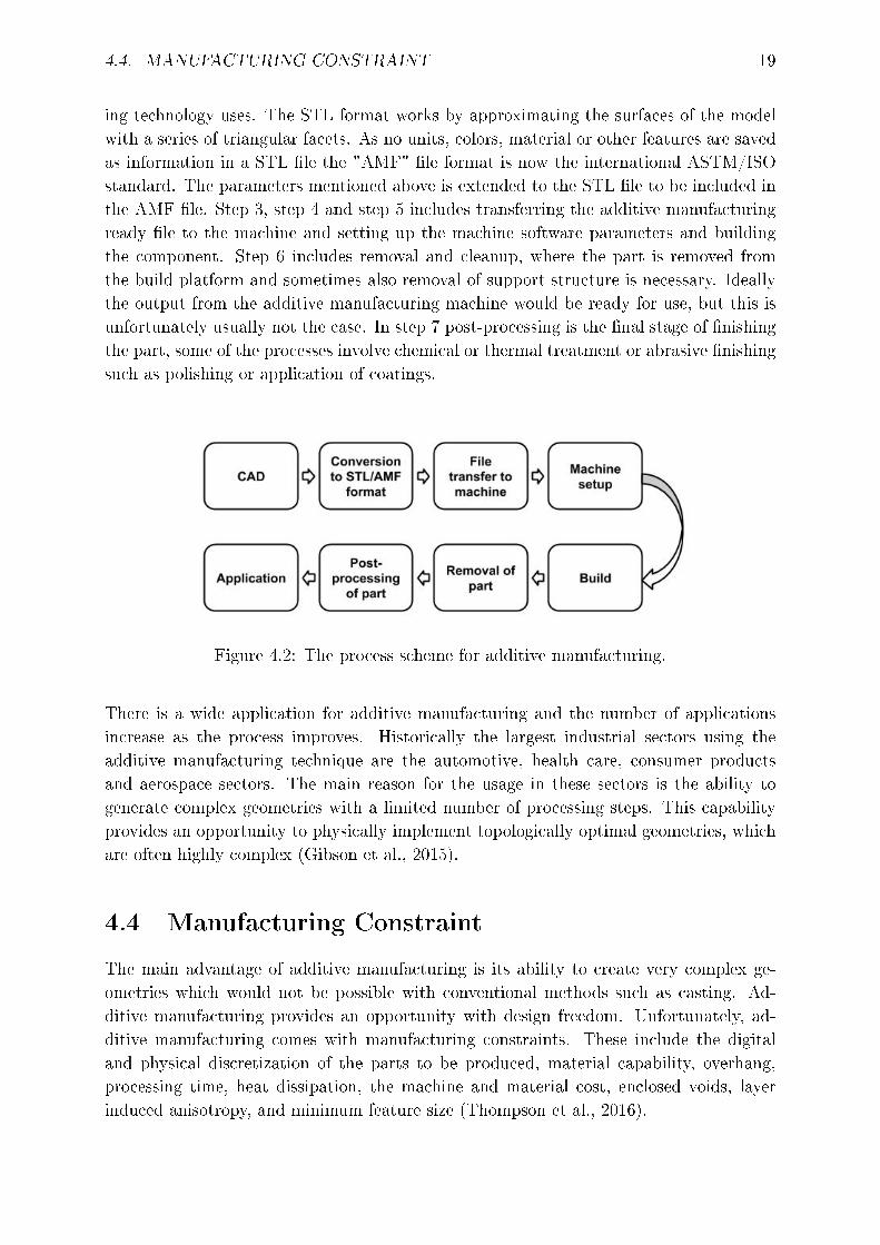
Gibson et al. (2015) have divided the general process chain for additive manufacturing
into eight steps. The process scheme can be observed in Figure 4.2. The rst step is to
obtain 3D CAD for instance through using a 3D CAD software. The next step will be to
convert the 3D CAD data to a STL le format, which nearly every additive manufactur-
Page 32
4.4. MANUFACTURING CONSTRAINT 19
ing technology uses. The STL format works by approximating the surfaces of the model
with a series of triangular facets. As no units, colors, material or other features are saved
as information in a STL le the "AMF" le format is now the international ASTM/ISO
standard. The parameters mentioned above is extended to the STL le to be included in
the AMF le. Step 3, step 4 and step 5 includes transferring the additive manufacturing
ready le to the machine and setting up the machine software parameters and building
the component. Step 6 includes removal and cleanup, where the part is removed from
the build platform and sometimes also removal of support structure is necessary. Ideally
the output from the additive manufacturing machine would be ready for use, but this is
unfortunately usually not the case. In step 7 post-processing is the nal stage of nishing
the part, some of the processes involve chemical or thermal treatment or abrasive nishing
such as polishing or application of coatings.
Figure 4.2: The process scheme for additive manufacturing.
There is a wide application for additive manufacturing and the number of applications
increase as the process improves. Historically the largest industrial sectors using the
additive manufacturing technique are the automotive, health care, consumer products
and aerospace sectors. The main reason for the usage in these sectors is the ability to
generate complex geometries with a limited number of processing steps. This capability
provides an opportunity to physically implement topologically optimal geometries, which
are often highly complex (Gibson et al., 2015).
4.4 Manufacturing Constraint
The main advantage of additive manufacturing is its ability to create very complex ge-
ometries which would not be possible with conventional methods such as casting. Ad-
ditive manufacturing provides an opportunity with design freedom. Unfortunately, ad-
ditive manufacturing comes with manufacturing constraints. These include the digital
and physical discretization of the parts to be produced, material capability, overhang,
processing time, heat dissipation, the machine and material cost, enclosed voids, layer
induced anisotropy, and minimum feature size (Thompson et al., 2016).
Page 33
20 CHAPTER 4. ADDITIVE MANUFACTURING
Both polymer based processes and powdered metal based processes require support ma-
terial in order to ensure manufacturability for certain topologies. For example the FDM
method, the DMLS method and the SLM method require support structures in order
to be able to manufacture certain topologies. In the FDM method support structures
surround the the part. It prevents the structural material from distorting for instance
through curling because of residual stresses or sagging due to unsupported regions. The
support material is removed in a post-print chemical bath. The usage of support struc-
tures increase the material usage, print time and require a chemical bath for removal
(Vanek et al., 2014). Vanek et al. (2014) denes the critical angle for the FDM process
where support structures are needed to 45, i.e. the printing faces may deviate up to 45
from the printing direction vector in order to be printable without support structures. It
is however pointed out that the exact value of the critical angle varies from printer to
printer and is not generally accessible.
Metal additive manufacturing, MAM, usually requires support structures to hold the
part during the process. The thermal gradient from the selective heating and solidica-
tion processes creates residual stresses that leads to signicant distortions such as curing
and warping in the part (Thomas, 2010). It has been shown that overhanging surfaces
warp easier when the inclined angle is smaller. Other parameters such as scanning speed
and laser power also aect warping (Wang et al., 2013). The aect of the need of support
structures for MAM is similar to when using polymers, it increases the material usage,
the print time and the post-fabrication time. The support structures connect the build
platform to the part which provides structural resistance against distortion and help with
the heat dissipation. By preventing overhang features in the design one might be able
to be avoided support stuctures (Thomas, 2010). Thomas (2010) identies the typical
critical angle as to 45 in the DMLS process and Wang et al. (2013) identies the critical
angle to 45 in the SLM process.
Page 34
Chapter 5
Topology Optimization for Additive
Manufacturing
Topology optimization results in an optimal material distribution that is independent of
a priori assumption of domain connectivity, and therefore provides an opportunity for
innovative structural design. The design obtained from topology optimization is usually
very complex. Traditional manufacturing techniques are expensive, and will in some cases
even fail, with higher demands on the complexity of the structure. However, when using
additive manufacturing this is not the case. Due to the many manufacturing constraints
using conventional manufacturing processes the optimized topology requires simplication
or constraining of the design space. Combining topology optimization with the design
freedom that comes with additive manufacturing could create the perfect couple. Even
though the number of constraints in additive manufacturing is not as many as with con-
ventional manufacturing methods they still need to be taken into account. Clausen (2016)
divides the constraints into two categories for additive manufacturing oriented topology
optimization. The rst one is the non-directional constraints which include enclosed voids
and minimum feature size. The second category are the directional constraints, charac-
terized by being related to the print direction. Examples of the directional constraints
are the layer induced anisotropy, thermal warping and overhang support. There are a
few methods where the topology optimization algorithm is combined with constraints
regarding additive manufacturing.
5.1 Non-directional constraints
Enclosed voids is a constraint for certain additive manufacturing technologies, eg. SLM
and SLS, where powder gets trapped inside the void or FDM. In the FDM method sup-
port structures are usually necessary inside a part which are needed to be removed after
manufacturing. Various approaches have been suggested to implement this constraint
in topology optimization. Shutian et al. (2015) suggested an approach named virtual
temperature method (VTM). The voids in the structure are lled with a virtual heating
material with high heat conductivity and solid areas are lled with a virtual material with
low heat conductivity. The constraint is integrated as a maximum temperature constraint
21
Page 35
22CHAPTER 5. TOPOLOGYOPTIMIZATION FORADDITIVEMANUFACTURING
and can be used as a constraint in topology optimization. Quhao et al. (2016) continues
on this approach proposing the generalized method, virtual scalar eld method (VSFM)
where the temperature eld could be one of the scalar elds.
The minimum feature size constraint in additive manufacturing could be compared with
the minimum member thickness constraint investigated by Guest et al. (2004) and Poulsen
(2003). Poulsen (2003) presents a scheme to implement a minimum length scale in topol-
ogy optimization. It depends on testing for monotonicity of the restriction of the density
function to test lines and is formulated as one constraint. Guest et al. (2004) uses nodal
design variables projected by functions based on the minimum length scale onto element
space determining the element volume fraction. A more recent publication by Zhou et al.
(2015) have presented an approach to achieve minimum length scale based on geometric
constraints in a ltering-threshold topology optimization scheme. The approach is based
on a density lter combined with a projection scheme. This sort of constraint is also
found in commercial softwares such as in OptiStruct by Altair (OptiStruct, 2017).
5.2 Directional constraints
The so called directional constraints dened by Clausen (2016) cause a bit more incon-
venience because the print direction plays a huge roll. According to Clausen (2016) the
print direction should also be optimized. All the directional constraints such as layer
induced anisotropy, thermal warping and overhang should be included to optimize the
orientation in which the part should be printed. Thermally induced residual stresses, or
thermal warping, come from local melting and nonuniform cooling of the part. The need
for support structures in metal printing is mainly due to thermal induced residual stresses
and heat dissipation. Li et al. (2016) developed two multiscale modeling methods to be
able to predict residual stresses in the parts. The proposed methods are however not
validated in reality. The result of layer induced anisotropy is that for certain additive
manufacturing methods the print direction will be weaker than the in-plane direction.
This could be included in topology optimization using an orthotropic material with one
weaker direction and one stier direction which is not a problem if the print direction is
predened (Clausen, 2016).
There are a few methods including a constraint to achieve self-supporting structures
without support structures. Brackett et al. (2011) provided an overview of the issues
and opportunities for application of topology optimization for additive manufacturing. It
was proposed that an overhang detection procedure was to be integrated in the topology
optimization but no result was reported. Leary et al. (2014) presented a novel method
that modies the theoretically optimal topology to enable additive manufacturing. The
method focus on the FDM method which has a problem with overhang. The inclina-
tion angle between the plate and the surface was divided into three zones; robust zone
(40 ≤ θ), compromised zone (30 ≤ θ < 40) and failed zone (θ < 30). The reported result
ensured manufacturability without support material.
Page 36
5.2. DIRECTIONAL CONSTRAINTS 23
Gaynor and Guest (2016) embedded a minimum allowable self-supporting angle extend-
ing the ltering procedure, through a series of projection operations, making the part self
supporting. A combination of local projection to enforce minimum length scale and sup-
port region projection address both the minimum feature size constraint and the overhang
constraint. The lter mimics the actual additive manufacturing process as it is applied in
a layer-wise manner which according to Gaynor and Guest (2016) is one of two primary
disadvantages. This generally result in computational ineciency since ecient parallel
processing can not be utilized with this approach. The method is based on the regularized
Heaviside projection method by Guest et al. (2004). It uses two neighbourhood sets, one
with the local neighbourhood within a distance, rmin, of the element centroid and one set
related to the overhang conditions dened as the region that must contain some material
for the point to be considered supported. The latter set is limited to those points within
a distance, rs, below the design variable i creating a wedge-shaped region. The ltered
density variables are a function of embedded non-linear functions which lead to the sec-
ond primary disadvantage with the method according to Gaynor and Guest (2016). Thus
it leads to convergence issues for more dicult design problems. The published result
show that the generated designs are self supporting. However, in need of an additional
projection step to remove intermediate densities.
Langelaar (2017) presents a method that can be included in conventional density-based
topology optimization. All the elements in the mesh is associated with a blueprint density
and gets printed if they are suciently supported. Langelaar (2017) targets the SLM and
EBM additive manufacturing process where, as mentioned before, the critical angle is
αc = 45. The supported region for a element for the two dimensional case is the three
elements below it. This result in that if the angle is set to 45 it has to be square elements.The lter works in a way such that the printed density can't be larger than the maxi-
mum density in the supporting region. This results in elements that are not suciently
supported do not get printed. The reported result show that the models become self
supporting but some regions contain intermediate densities and an additional projection
step is necessary to get rid of these regions. The additive manufacturing lter has also
been extended to the three dimensional case by Langelaar (2016). It works in a similar
way as for the two dimensional case, however, the support region now contain the nine
elements below. The method presented in Langelaar (2017) for the two dimensional case
will be further evaluated in Chapter 6.
Page 37
Chapter 6
Evaluation of Existing Method
Langelaar (2017) presents a method that can very easily be integrated in a density-
based topology optimization algorithm. The method takes the overhang constraint into
account, especially targeting SLM and EBM additive manufacturing processes, and the
lter mimics the additive manufacturing process by being applied in a layer-by-layer
manner.
6.1 Method and Derivation
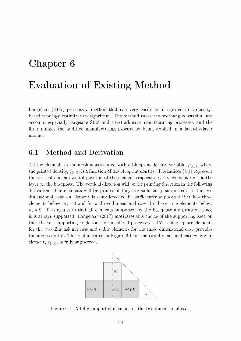
All the elements in the mesh is associated with a blueprint density variable, ρ(i,j), wherethe printed density, ξ(i,j), is a function of the blueprint density. The indices (i, j) representthe vertical and horizontal position of the element respectively, i.e. element i = 1 is the
layer on the baseplate. The vertical direction will be the printing direction in the following
derivation. The elements will be printed if they are suciently supported. In the two
dimensional case an element is considered to be suciently supported if it has three
elements below, ns = 3 and for a three dimensional case if it have nine elements below,
ns = 9. This results in that all elements supported by the baseplate are printable since
it is always supported. Langelaar (2017) motivates this choice of the supporting area on
that the self supporting angle for the considered processes is 45. Using square elements
for the two dimensional case and cubic elements for the three dimensional case provides
the angle α = 45. This is illustrated in Figure 6.1 for the two dimensional case where an
element, e(i,j), is fully supported.
Figure 6.1: A fully supported element for the two dimensional case.
24
Page 38
6.1. METHOD AND DERIVATION 25
Elements located on the far left or far right edge will be taken into account for in the
implementation as they are supported with two elements for the two dimensional case.
This is done by adding an extra element with the value zero on each side. For elements
i ≠ 1, i.e. not on the baseplate, the element printed density is dened through that it
can't be higher than the maximum printed density Ξ(i,j) in the supporting region. This
is expressed as
ξ(i,j) =min (ρ(i,j),Ξ(i,j)) (6.1)
Ξ(i,j) =max (ξ(i−1,j−1), ξ(i−1,j), ξ(i−1,j+1)) (6.2)
As gradient information is essential in the topology optimization, Langelaar (2017) ap-
proximate the non-smooth functions in (6.1) and (6.2) as
smin(ρ(i,j),Ξ(i,j)) ≡1
2(ρ(i,j) +Ξ(i,j) − ((ρ(i,j) −Ξ(i,j))
2+ ε)
12+√ε) = ξ(i,j) (6.3)
smax(ξ(i−1,j−1), ξ(i−1,j), ξ(i−1,j+1)) ≡ (ξP(i−1,j−1) + ξP(i−1,j) + ξ
P(i−1,j+1))
1Q= Ξ(i,j) (6.4)
where Q = P +log(ns)
log(ξ0)
The parameters P and ε in (6.3) and (6.4) controls the smoothness and accuracy of the
approximation. If the parameters ε → 0 and P → ∞ the exact minimum and maximum
operators are obtained. The default values for the parameters are set to ε = 10−4, P = 40
and ξ0 = 0.5. Consider an objective function to be minimized with a given constraint.
The objective function depend on the printed geometry which in turn depend on the blue
print design, C(ξξξ(ρρρ)). The chain rule provides
∂C
∂ρρρ= [
∂C
∂ξξξ
∂ξξξ
∂ρρρ]∂ρρρ
∂ρρρ(6.5)
The ltered blueprint design eld using a density lter is dened according to equation
(3.32) and here becomes
ρρρe =∑we,iviρi
∑we,ivi(6.6)
The rst two parts in (6.5) are derived by combining (6.3) and (6.4), such that smin (ρρρi, ξξξi−1)−
ξξξi = 0, and using this as the constraint equation. ξξξi−1 is used because the printed density
depend on the supporting region below. For eciency the adjoint method is utilized.
The augmented response of the objective function, C(ξξξ(ρρρ)), and the constraint function
becomes
C = C(ξξξ(ρρρ)) +ni
∑i=1
λλλTi (smin(ρρρi, ξξξi−1) − ξξξi) (6.7)
Page 39
26 CHAPTER 6. EVALUATION OF EXISTING METHOD
where λλλi are the adjoint vectors. At the rst layer, right above the baseplate, dierentia-
tion of equation (6.7) and dening ξξξ1 = smin,1 ≡ ρρρ1 provides the following expression
∂C
∂ρρρj=
ni
∑i=1
[∂C
∂ξξξi
∂ξξξi∂ρρρj
+λλλTi (∂smin,i∂ρρρj
δij +∂smin,i∂ξξξi−1
∂ξξξi−1
∂ρρρj−∂ξξξi∂ρρρj
)] (6.8)
The printed densities only depend on the blueprint density and the result of this is ∂ξξξi∂ρρρj
= 0
for i < j. Using the constraint mentioned above, moving terms with i = j outside of the
summation and writing the last term in the summation as a separate sum provides
∂C
∂ρρρj=∂C
∂ξξξj
∂ξξξj∂ρρρj
+ni
∑i=j+1
(∂C
∂ξξξi−λλλi)
∂ξξξi∂ρρρj
+ni
∑i=j+1
(λλλTi∂smin,i∂ξξξi−1
∂ξξξi−1
∂ρρρj) (6.9)
From the second summation the rst term i = j + 1 is moved outside of the summation.
The remaining is reindexed and the last term in the rst sum is moved outside of the
summation making the two sums regain the same limits. Again using the constraint
mentioned above, equation (6.9) becomes
∂C
∂ρρρj= (
∂C
∂ξξξj+λλλTj+1
∂smin,j+1
∂ξξξj)∂smin,j∂ρρρj
+(∂C
∂ξξξni−λλλTni)
∂ξξξni∂ρρρj
+ni−1
∑i=j+1
(∂C
∂ξξξi−λλλTi +λλλ
Ti+1
∂smin,i+1
∂ξξξi)∂ξξξi∂ρρρj
(6.10)
Equation (6.10) holds for 1 ≤ j ≤ ni and in order to simplify the calculations λλλi and λλλniare chosen in the following manner
λλλTj =∂C
∂ξξξj+λλλTj+1
∂smin,j+1
∂ξξξjfor 1 ≤ j < ni λλλTni =
∂C
∂ξξξni(6.11)
The multipliers above avoids calculations of the term ∂ξξξi∂ρρρ . The term
∂C∂ξξξj
will be similar to
the rst part in (3.34) but with respect to the printed density, ξj, if the SIMP method is
used. Equation(6.10) together with the multipliers in (6.11) becomes
∂C
∂ρρρj=∂C
∂ρρρj= (
∂C
∂ξξξj+λλλTj+1
∂smin,j+1
∂ξξξj)∂smin,j∂ρρρj
= λλλTj∂smin,j∂ρρρj
(6.12)
It can be observed that each multiplier depend on the layer above. This results in that
the algorithm start at the top layer and moves down. The following expressions are used
when calculating the derivatives of smin in (6.12) and are derived using (6.3), and (6.4).
∂smin(x,Ξ)
∂ρ=
1
2(1 − (ρ −Ξ) ((ρ −Ξ)2 + ε)
− 12) (6.13)
∂smin∂ξ
=∂smin∂Ξ
∂Ξ
∂ξwhere
⎧⎪⎪⎪⎨⎪⎪⎪⎩
∂smin(ρ,Ξ)∂Ξ = 1
2 (1 + (ρ −Ξ) ((ρ −Ξ)2 + ε)− 1
2)
∂Ξ(ξ1,ξ2,ξ3)∂ξi
=PξP−1i
Q(∑
nsk=1 ξ
Pk )
1Q−1 (6.14)
The last part in (6.5) is the same expression calculated in the sensitivity analysis for the
density lter in Section 3.4, i.e. the second part in (3.34), and is derived from equation
Page 40
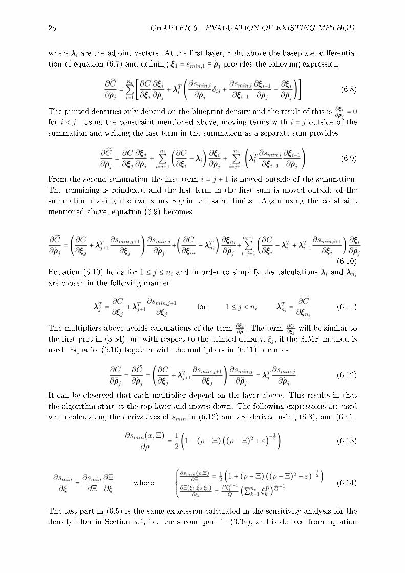
6.2. PERFORMANCE AND RESULT 27
(6.6). With the considered method four dierent printing directions can be examined due
to the denition of the supported region. These are depicted in Figure 6.2.
Figure 6.2: Baseplates for the additive manufacturing lter.
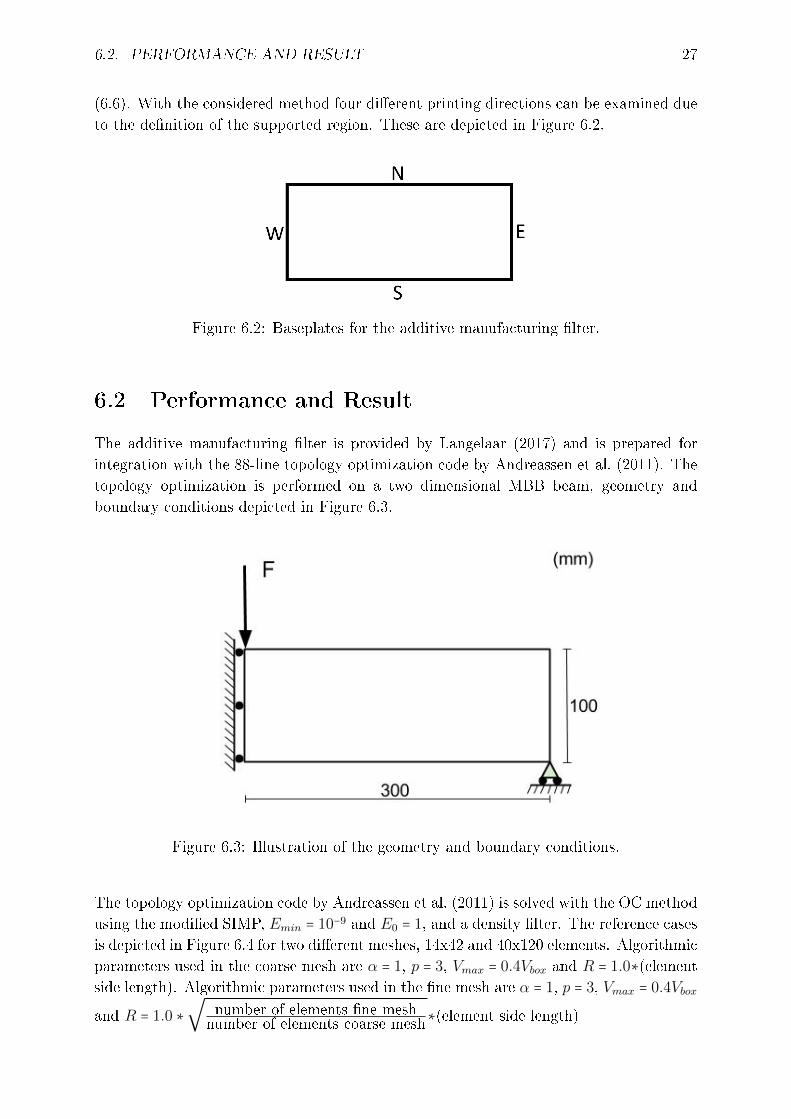
6.2 Performance and Result
The additive manufacturing lter is provided by Langelaar (2017) and is prepared for
integration with the 88-line topology optimization code by Andreassen et al. (2011). The
topology optimization is performed on a two dimensional MBB beam, geometry and
boundary conditions depicted in Figure 6.3.
Figure 6.3: Illustration of the geometry and boundary conditions.
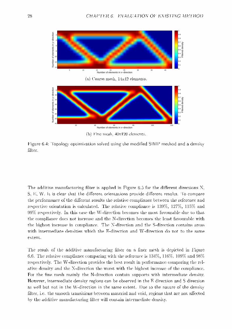
The topology optimization code by Andreassen et al. (2011) is solved with the OC method
using the modied SIMP, Emin = 10−9 and E0 = 1, and a density lter. The reference cases
is depicted in Figure 6.4 for two dierent meshes, 14x42 and 40x120 elements. Algorithmic
parameters used in the coarse mesh are α = 1, p = 3, Vmax = 0.4Vbox and R = 1.0∗(element
side length). Algorithmic parameters used in the ne mesh are α = 1, p = 3, Vmax = 0.4Vbox
and R = 1.0 ∗
√number of elements ne meshnumber of elements coarse mesh∗(element side length)
Page 41
28 CHAPTER 6. EVALUATION OF EXISTING METHOD
Number of elements in x−direction
Num
ber
of e
lem
ents
in y
−di
rect
ion
5 10 15 20 25 30 35 40
2
4
6
8
10
12
14
Filt
ered
den
sity
0
0.1
0.2
0.3
0.4
0.5
0.6
0.7
0.8
0.9
1
(a) Coarse mesh, 14x42 elements.
Number of elements in x−direction
Num
ber
of e
lem
ents
in y
−di
rect
ion
20 40 60 80 100 120
5
10
15
20
25
30
35
40
Filt
ered
den
sity
0
0.1
0.2
0.3
0.4
0.5
0.6
0.7
0.8
0.9
1
(b) Fine mesh, 40x120 elements.
Figure 6.4: Topology optimization solved using the modied SIMP method and a density
lter.
The additive manufacturing lter is applied in Figure 6.5 for the dierent directions N,
S, E, W. It is clear that the dierent orientations provide dierent results. To compare
the performance of the dierent results the relative compliance between the reference and
respective orientation is calculated. The relative compliance is 139%, 127%, 115% and
99% respectively. In this case the W-direction becomes the most favourable due to that
the compliance does not increase and the N-direction becomes the least favourable with
the highest increase in compliance. The N-direction and the S-direction contains areas
with intermediate densities which the E-direction and W-direction do not to the same
extent.
The result of the additive manufacturing lter on a ner mesh is depicted in Figure
6.6. The relative compliance comparing with the reference is 134%, 116%, 109% and 98%
respectively. The W-direction provides the best result in performance comparing the rel-
ative density and the N-direction the worst with the highest increase of the compliance.
For the ne mesh mainly the N-direction contain supports with intermediate density.
However, intermediate density regions can be observed in the E-direction and S-direction
as well but not in the W-direction in the same extent. Due to the nature of the density
lter, i.e. the smooth transitions between material and void, regions that are not aected
by the additive manufacturing lter will contain intermediate density.
Page 42
6.2. PERFORMANCE AND RESULT 29
Number of elements in x−direction
Num
ber
of e
lem
ents
in y
−di
rect
ion
5 10 15 20 25 30 35 40
2
4
6
8
10
12
14
Filt
ered
den
sity
0
0.1
0.2
0.3
0.4
0.5
0.6
0.7
0.8
0.9
1
(a) Coarse mesh, N-direction. CCref
= 1.39
Number of elements in x−direction
Num
ber
of e
lem
ents
in y
−di
rect
ion
5 10 15 20 25 30 35 40
2
4
6
8
10
12
14
Filt
ered
den
sity
0
0.1
0.2
0.3
0.4
0.5
0.6
0.7
0.8
0.9
1
(b) Coarse mesh, S-direction. CCref
= 1.27
Number of elements in x−direction
Num
ber
of e
lem
ents
in y
−di
rect
ion
5 10 15 20 25 30 35 40
2
4
6
8
10
12
14
Filt
ered
den
sity
0
0.1
0.2
0.3
0.4
0.5
0.6
0.7
0.8
0.9
1
(c) Coarse mesh, E-direction. CCref
= 1.15
Number of elements in x−direction
Num
ber
of e
lem
ents
in y
−di
rect
ion
5 10 15 20 25 30 35 40
2
4
6
8
10
12
14
Filt
ered
den
sity
0
0.1
0.2
0.3
0.4
0.5
0.6
0.7
0.8
0.9
1
(d) Coarse mesh, W-direction. CCref
= 0.99
Figure 6.5: Additive manufacturing lter by Langelaar (2017) applied on the coarse mesh.
Page 43
30 CHAPTER 6. EVALUATION OF EXISTING METHOD
Number of elements in x−direction
Num
ber
of e
lem
ents
in y
−di
rect
ion
20 40 60 80 100 120
5
10
15
20
25
30
35
40
Filt
ered
den
sity
0
0.1
0.2
0.3
0.4
0.5
0.6
0.7
0.8
0.9
1
(a) Fine mesh, N-direction. CCref
= 1.34
Number of elements in x−direction
Num
ber
of e
lem
ents
in y
−di
rect
ion
20 40 60 80 100 120
5
10
15
20
25
30
35
40
Filt
ered
den
sity
0
0.1
0.2
0.3
0.4
0.5
0.6
0.7
0.8
0.9
1
(b) Fine mesh, S-direction. CCref
= 1.16
Number of elements in x−direction
Num
ber
of e
lem
ents
in y
−di
rect
ion
20 40 60 80 100 120
5
10
15
20
25
30
35
40F
ilter
ed d
ensi
ty0
0.1
0.2
0.3
0.4
0.5
0.6
0.7
0.8
0.9
1
(c) Fine mesh, E-direction. CCref
= 1.09
Number of elements in x−direction
Num
ber
of e
lem
ents
in y
−di
rect
ion
20 40 60 80 100 120
5
10
15
20
25
30
35
40
Filt
ered
den
sity
0
0.1
0.2
0.3
0.4
0.5
0.6
0.7
0.8
0.9
1
(d) Fine mesh, W-direction. CCref
= 0.99
Figure 6.6: Additive manufacturing lter by Langelaar (2017) applied on the ne mesh.
A dierent topology can be observed for each direction comparing with the topology in
the coarse mesh. This is probably the eect of how an element is distinguished to be
supported. A compiled result of the relative compliance for the two meshes is presented
in Table 6.1. The W-direction provides the best result and the N-direction the worst
result regarding the relative compliance in both meshes. The relative compliance for the
Page 44
6.2. PERFORMANCE AND RESULT 31
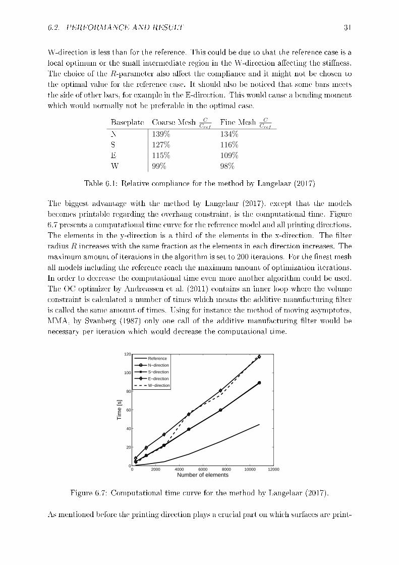
W-direction is less than for the reference. This could be due to that the reference case is a
local optimum or the small intermediate region in the W-direction aecting the stiness.
The choice of the R-parameter also aect the compliance and it might not be chosen to
the optimal value for the reference case. It should also be noticed that some bars meets
the side of other bars, for example in the E-direction. This would cause a bending moment
which would normally not be preferable in the optimal case.
Baseplate Coarse Mesh CCref
Fine Mesh CCref
N 139% 134%
S 127% 116%
E 115% 109%
W 99% 98%
Table 6.1: Relative compliance for the method by Langelaar (2017)
The biggest advantage with the method by Langelaar (2017), except that the models
becomes printable regarding the overhang constraint, is the computational time. Figure
6.7 presents a computational time curve for the reference model and all printing directions.
The elements in the y-direction is a third of the elements in the x-direction. The lter
radius R increases with the same fraction as the elements in each direction increases. The
maximum amount of iterations in the algorithm is set to 200 iterations. For the nest mesh
all models including the reference reach the maximum amount of optimization iterations.
In order to decrease the computational time even more another algorithm could be used.
The OC optimizer by Andreassen et al. (2011) contains an inner loop where the volume
constraint is calculated a number of times which means the additive manufacturing lter
is called the same amount of times. Using for instance the method of moving asymptotes,
MMA, by Svanberg (1987) only one call of the additive manufacturing lter would be
necessary per iteration which would decrease the computational time.
0 2000 4000 6000 8000 10000 120000
20
40
60
80
100
120
Number of elements
Tim
e [s
]
Reference
N−direction
S−direction
E−direction
W−direction
Figure 6.7: Computational time curve for the method by Langelaar (2017).
As mentioned before the printing direction plays a crucial part on which surfaces are print-
Page 45
32 CHAPTER 6. EVALUATION OF EXISTING METHOD
able. This is very easily veried when comparing the relative compliance and topologies
for the dierent directions retrieved with the additive manufacturing lter. This leads
to a major disadvantage of this method where the additive manufacturing lter requires
the print direction to be axiparallel to the coordinate axis. This might be circumvented
through isoparametric formulation and element mapping, but would complicate the calcu-
lations and consequently the computation time would increase. The same constraint, i.e.
the support region tied to the element discretization, leads to the next big disadvantage.
The self supporting angle is tied to the aspect ratio of the elements. In order to analyze
an angle dierent from 45 the ratio between the element sides need to be changed. The
nature of the additive manufacturing lter lead to mesh dependence which is not desired.
To overcome this the denition of the supporting region need to be changed. The density
in an element should not only be dened by the density in adjacent elements. These
disadvantages should be further addressed to increase the usage of the lter. Finally, the
method requires information about neighbour elements which for ne meshes or complex
domains and geometries become very dicult to obtain thus it is an expensive operation.
During parallel computing, where the design domain is decomposed into partitions, the
complexity of problem increases further.
Page 46
Chapter 7
Density Gradient Method
The disadvantages regarding that the critical angle being tied to the aspect ratio of the
element, or the axiparallel print direction in the additive manufacturing lter by Langelaar
(2017) could be further addressed using the same method. However, in order to address
the constraint with the requirement of neighbour elements the entire formulation needs
to be changed. As mentioned before the density lter as a solution of Helmholtz PDE by
Lazarov and Sigmund (2011) does not require this sort of information about the neighbour
elements, thus could become more advantageous to use for a ner or more complicated
mesh.
7.1 Density Gradient
The same idea as when calculating the temperature gradient in two dimensional heat ow
is used when calculating the density gradient. For a four-node rectangular element the
boundaries must be parallel to the coordinate system. In order to get a more generalized
formulation the density gradient is derived for a four-node isoparametric quadrilateral
element and the mapping is illustrated in Figure 7.1.
Figure 7.1: Illustation of an element mapping.
The density gradient in two dimensions is
∇∇∇ρ =
⎡⎢⎢⎢⎢⎣
∂ρ∂x
∂ρ∂y
⎤⎥⎥⎥⎥⎦
(7.1)
33
Page 47
34 CHAPTER 7. DENSITY GRADIENT METHOD
The shape functions for a four-node isoparametric quadrilateral element are
N e1 =
1
4(ξ − 1)(η − 1)
N e2 = −
1
4(ξ + 1)(η − 1) (7.2)
N e3 =
1
4(ξ + 1)(η + 1)
N e4 = −
1
4(ξ − 1)(η + 1)
The mapping between the coordinate systems is obtained through
x = x(ξ, η) =NNN e(ξ, η)xxxe y = y(ξ, η) =NNN e(ξ, η)yyye (7.3)
where
NNN e(ξ, η) = [N e1 N e
2 N e3 N e
4 ] , xxxe =
⎡⎢⎢⎢⎢⎢⎢⎢⎢⎣
x1
x2
x3
x4
⎤⎥⎥⎥⎥⎥⎥⎥⎥⎦
, yyye =
⎡⎢⎢⎢⎢⎢⎢⎢⎢⎣
y1
y2
y3
y4
⎤⎥⎥⎥⎥⎥⎥⎥⎥⎦
(7.4)
The approximation of the density is
ρ = ρ(ξ, η) =NNN e(ξ, η)ρρρ where ρρρ = [ρ1 ρ2 ρ3 ρ4] (7.5)
Equation (7.1) can be rewritten using the approximation in (7.5) and becomes
∇∇∇ρ =
⎡⎢⎢⎢⎢⎣
∂NNNe
∂x
∂NNNe
∂y
⎤⎥⎥⎥⎥⎦
ρρρ = (JJJT )−1
⎡⎢⎢⎢⎢⎣
∂NNNe
∂ξ
∂NNNe
∂η
⎤⎥⎥⎥⎥⎦
ρρρ where JJJ =
⎡⎢⎢⎢⎢⎣
∂x∂ξ
∂x∂η
∂y∂ξ
∂y∂η
⎤⎥⎥⎥⎥⎦
(7.6)
7.2 Additive Manufacturing Filter
In Figure 7.2 the gradient vector and the normal to the baseplate are illustrated. The gra-
dient vector represents the gradient of the ltered density variables. Using the denition
of the scalar product, in equation (7.7), the angle between the normal to the baseplate
and the density gradient can be calculated
θ = arccos(vvvT∇∇∇ρ
∣∣vvv∣∣ ∣∣∇∇∇ρ∣∣) (7.7)
If using the fact that the normal to the baseplate, vvv, is [0,1,0], the elements with angles
less than the critical angle can be determined. If an angle θ0 is dened as the critical
angle the angles smaller than this is at risk, i.e. θ ≤ θ0 interfere with the constraint. This
is illustrated in Figure 7.2 where the green line represents the smallest allowed angle and
the red line represents an angle smaller than the minimum allowed angle.
Page 48
7.2. ADDITIVE MANUFACTURING FILTER 35
Figure 7.2: Illustration of the density gradient constraint.
7.2.1 Formulation
In the same manner as when using the energy balance (strong form) to obtain the mini-
mization of the functional for heat conduction and the principle of virtual temperatures
the PDE lter could be examined.
−∇∇∇TKKKd∇∇∇ρ + ρ = ρ (7.8)
The strong form of (7.8) is
div(−KKKd∇∇∇ρ) + ρ = ρ (7.9)
The potential associated with (7.9)
Π(ρ) = ∫V
1
2(∇∇∇ρ)TKKKd∇∇∇ρdV + ∫
V
1
2(ρ − ρ)2dV − ∫
∂VρqndS (7.10)
where the last part vanishes since qn = 0 on ∂S. Moreover, if the function w = 12∇∇∇ρ
TKKKd∇∇∇ρ
is dened, where KKKd is positive denite, the functional in (7.10) becomes
Π(ρ) = ∫Vw(∇∇∇ρ)dV + ∫
V
1
2(ρ − ρ)2dV (7.11)
and the minimization of the functional is
δΠ = ∫V
∂w
∂∇∇∇ρδ(∇∇∇ρ)dV − ∫
V(ρ − ρ)δρdV (7.12)
Upon using qi = ( ∂w∂∇∇∇ρ), equation (7.12) can be expressed as
δΠ = ∫Vqi∂
∂xi(δρ)dV − ∫
V(ρ − ρ)δρdV (7.13)
Making use of ∫V (qiδρ),i dV = ∫∂V qiδρnidS = 0 where the last equality holds due to qi=0
provides after some calculation the weak form
∫V−v,iqidV + ∫
VvρdV = ∫
Vvρ (7.14)
For the FE-formulation of the weak form of the lter equation (7.14) the following nota-
tions is used ρe =NNN eρρρ, vvv =NNN eccc, ∇∇∇v =BBBeccc and equation (7.14) takes the form
Page 49
36 CHAPTER 7. DENSITY GRADIENT METHOD
∫VBBBTqqqdV + ∫
VNNNTNNNdV ρρρ = ∫
VNNNTdV ρρρ (7.15)
With MMM = ∫V NNNTNNNdV and TTT = ∫V NNN
TdV equation (7.15) becomes
RRR(ρρρ,ρρρ) = ∫VBBBTqqqdV +MMMρρρ −TTTρρρ = 000 (7.16)
In order to change the nature of the lter the function w(∇∇∇ρ) could be changed, for in-
stance to a non-linear function.
To solve this system of potentially non-linear equations Newton Raphson's method could
be used. Newton Raphson's method makes use of the known solution from the previous
iteration, n, to solve the current iteration, n+1. Taylor's rst order approximation of the
residual function is
RRRn+1(ρρρn+1,ρρρ) =RRRn(ρρρn,ρρρ) +∂RRRn(ρρρn,ρρρ)
∂ρρρn(ρρρn+1 − ρρρn) = 000 (7.17)
Using that the residual in the updated state, RRRn+1(ρρρn+1,ρρρ), is small compared with the
previous state , RRRn(ρρρn,ρρρ), the ltered densities from the current iteration can be solved
from
ρρρn+1 = ρρρn − (∂RRRn(ρρρn,ρρρ)
∂ρρρn)
−1
RRRn(ρρρn,ρρρ) (7.18)
The residual function can be updated using the new ρρρn+1. If RRRn+1(ρρρn+1,ρρρ) > tolerance
the next iteration, n = n + 1, will be calculated. The derivative of the lter function with
respect to the ltered density, ρρρ, needs to be calculated and becomes
∂RRR(ρρρ,ρρρ)
∂ρρρ= ∫
VBBBT ∂qqq
∂ρρρdV +MMM = 000 (7.19)
With KKKd =∂qi∂∇∇∇ρρρ equation (7.19) becomes
∂RRR(ρρρ,ρρρ)
∂ρρρ= ∫
VBBBTKKKdBBBdV +MMM = 000 (7.20)
7.2.2 Sensitivity Analysis
The lter is expressed as
RRR(ρρρ,ρρρ) = 000 (7.21)
The sensitivity analysis is performed using the adjoint method. The objective function,
g, including the non linear lter can be written as
g = FFF Tuuu(ρρρ) +λλλT (KKKuuu −FFF ) +ΛΛΛTRRR(ρρρ,ρρρ) (7.22)
where λλλ is the linear Lagrange multiplier and ΛΛΛ is the non linear Lagrange multiplier.
Dierentiation of (7.22) becomes
Page 50
7.2. ADDITIVE MANUFACTURING FILTER 37
∂g
∂ρρρ= FFF T ∂uuu
∂ρρρ+λλλT [
∂KKK
∂ρρρ
∂ρρρ
∂ρρρuuu +KKK
∂uuu
∂ρρρ] +ΛΛΛT [
∂RRR(ρρρ,ρρρ)
∂ρρρ
∂ρρρ
∂ρρρ+∂RRR(ρρρ,ρρρ)
∂ρρρ] (7.23)
In order to simplify the expression in (7.23) and to avoid calculations of the terms ∂uuu∂ρρρ and
∂ρρρ∂ρρρ it is rewritten to
∂g
∂ρρρ= [FFF T +λλλTKKK]
´¹¹¹¹¹¹¹¹¹¹¹¹¹¹¹¹¹¹¹¹¹¹¹¹¹¹¹¸¹¹¹¹¹¹¹¹¹¹¹¹¹¹¹¹¹¹¹¹¹¹¹¹¹¹¹¶=000
∂uuu
∂ρρρ+ [λλλT
∂KKK
∂ρρρuuu +ΛΛΛT ∂RRR(ρρρ,ρρρ)
∂ρρρ]
´¹¹¹¹¹¹¹¹¹¹¹¹¹¹¹¹¹¹¹¹¹¹¹¹¹¹¹¹¹¹¹¹¹¹¹¹¹¹¹¹¹¹¹¹¹¹¹¹¹¹¹¹¹¹¹¹¹¹¹¹¹¹¹¹¹¹¹¹¹¹¹¹¹¹¹¸¹¹¹¹¹¹¹¹¹¹¹¹¹¹¹¹¹¹¹¹¹¹¹¹¹¹¹¹¹¹¹¹¹¹¹¹¹¹¹¹¹¹¹¹¹¹¹¹¹¹¹¹¹¹¹¹¹¹¹¹¹¹¹¹¹¹¹¹¹¹¹¹¹¹¹¶=000
∂ρρρ
∂ρρρ+ΛΛΛT ∂RRR(ρρρ,ρρρ)
∂ρρρ(7.24)
Using the equilibrium equation the rst part provide the linear multiplier
FFF T +λλλTKKK = 000 Ô⇒ λλλT = −uuuT (7.25)
Using the linear multiplier in the second part provides the non linear multiplier
λλλT∂KKK
∂ρρρuuu +ΛΛΛT ∂RRR(ρρρ,ρρρ)
∂ρρρ= 000
Ô⇒ −uuuT∂KKK
∂ρρρuuu +ΛΛΛT ∂RRR(ρρρ,ρρρ)
∂ρρρ= 000
⇐⇒ ΛΛΛT = uuuT∂KKK
∂ρρρuuu(
∂RRR(ρρρ,ρρρ)
∂ρρρ)
−1
(7.26)
Now the sensitivity can be calculated and the only remaining part is the third part thus
it becomes
∂g
∂ρρρ= ΛΛΛT ∂RRR(ρρρ,ρρρ)
∂ρρρ(7.27)
For the conventional lter the function w(∇∇∇ρ) is
w =1
2∇∇∇ρρρTKKKd∇∇∇ρρρ (7.28)
The derivatives become
qi =∂w
∂∇∇∇ρρρ=KKKd∇ρ∇ρ∇ρ = r
2III∇ρ∇ρ∇ρ (7.29)
KKKd =∂qi∂∇∇∇ρρρ
=∂2w
∂∇∇∇ρρρ2= r2III (7.30)
The sensitivity using these functions become
∂g
∂ρ= ΛΛΛT ∂RRR(ρρρ, ρ)
∂ρ= −uuuT
∂KKK
∂ρρρuuu(KKK +MMM)−1TTT (7.31)
where KKK = ∫V
BBBTKKKdBBBdV ,MMM = ∫V
NNNTNNNdV and TTT = ∫V
NNNTdV . When comparing the expres-
sion in (7.31) with (3.45) and (3.46) in the regular density lter as a solution of Helmholtz
PDE these are the same, i.e. .
Page 51
38 CHAPTER 7. DENSITY GRADIENT METHOD
7.2.3 The Function w(∇∇∇ρ)
As mentioned before the nature of the lter could be changed by changing the function
w(∇∇∇ρ). It is dependent on the gradient of the ltered densities and using the denition
of the scalar product
cos(θ) = (vvvT∇∇∇ρ
∣∣vvv∣∣ ∣∣∇ρ∇ρ∇ρ∣∣) (7.32)
provides an expression depending on the gradient of the ltered densities and a vector,
vvvT = [x, y, z], describing a direction. An expression using the scalar product with a
function that reacts on for instance the critical angle and penalize angles below 45 couldbe formed. The function should almost act as a step function where if the angle between
the gradient and the baseplate is below a certain critical angle it should be penalized. To
get a smooth continuous function the following expression could be used
w(∇∇∇ρ) = r2 [arctan(z) + ez] where z = β [c + (vvv∇∇∇ρ
∣∣vvv∣∣ ∣∣∇∇∇ρ∣∣)] (7.33)
where β and c are constants used to control the position and rate of the function could be
chosen and the parameter r2 scales down the functions and could be related to the size
of the elements. The derivatives becomes
qi =∂w(∇∇∇ρ)
∂∇∇∇ρ= r3 [
1
1 + z2
∂z
∂∇∇∇ρ+ ez
∂z
∂∇∇∇ρ] (7.34)
KKKd =∂qi∂∇∇∇ρ
=∂2w(∇∇∇ρ)
∂∇∇∇ρ2= r3 [
1
1 + z2
∂2z
∂∇∇∇ρ2−
2 ∗ z
(1 + z2)2
∂z
∂∇∇∇ρ(∂z
∂∇∇∇ρ)
T
+
ez∂z
∂∇∇∇ρ(∂z
∂∇∇∇ρ)
T
+ ez∂2z
∂∇∇∇ρ2]
(7.35)
where
∂z
∂∇∇∇ρ= α [
vvv
∣∣vvv∣∣ ∣∣∇∇∇ρ∣∣−
(∇∇∇ρ)Tvvv(∇∇∇ρ)
∣∣vvv∣∣ ∣∣∇∇∇ρ∣∣3] (7.36)
∂2z
∂∇∇∇ρ2= −α [
vvv(∇∇∇ρ)T
∣∣vvv∣∣ ∣∣∇∇∇ρ∣∣3+
(∇∇∇ρ)vvvT
∣∣vvv∣∣ ∣∣∇∇∇ρ∣∣3+
(∇∇∇ρ)TvvvIII
∣∣vvv∣∣ ∣∣∇∇∇ρ∣∣3− 3
(∇∇∇ρ)Tvvv(∇∇∇ρ)(∇∇∇ρ)T
∣∣vvv∣∣ ∣∣∇∇∇ρ∣∣5] (7.37)
By choosing the function w(∇∇∇ρ) as in equation (7.33) it acts as a step-function similar
to the thresholding functions. Increasing the parameter β will provide a steeper slope
thus aect the function more. The parameter c acts as the thresholding parameter and
could be chosen to the value of the critical angle. From Figure 7.2 it is clear that in
order to not violate the overhang constraint θ0 ≤ θ which leads to cos(θ) ≤ cos(θ0) which
is illustrated in Figure 7.3a. In Figure 7.3b the function w(∇∇∇ρ) is plotted according to
equation (7.33) with the parameters: vvvT = [0,1], c = − cos(45) and, β = 10 for the lower
curve and vvvT = [0,1], c = − cos(45) and, β = 11 for the higher curve.
Page 52
7.3. RESULT AND PERFORMANCE 39
-200 -150 -100 -50 0 50 100 150 200
Angle, θ
-1
-0.8
-0.6
-0.4
-0.2
0
0.2
0.4
0.6
0.8
1co
s(θ)
(a) cos(θ)
0 20 40 60 80 100 120 140 160 180−2
0
2
4
6
8
10
12
14
16x 10
7
Angle
W
(b) The function w(∇∇∇ρ)
Figure 7.3: Filter equation w(∇∇∇ρ).
7.3 Result and performance
The topology optimization is performed on a two dimensional MBB beam, where ge-
ometry and boundary conditions are depicted in Figure 7.4. The compliance is to be
minimized with a volume constraint. The element discretization is performed with four-
node rectangular elements.
Figure 7.4: Illustration of the geometry and boundary conditions.
Figure 7.5a and Figure 7.5b show the result from the topology optimization solved using
the MMA described in Section 3.2 for two dierent meshes, 14x42 and 40x120 elements.
It has been solved using the SIMP approach described in Section 3.3 with the algorithmic
parameter p = 3 and with modulus of elasticity E = 1. It can be observed that the numer-
ical problems mentioned in Section 3.4 do appear in the solution. There are checkerboard
regions where the solid and void alternates, mainly observed with the ner mesh in Fig-
ure 7.5b. Figure 7.5c and Figure 7.5d depicts the ltered design using Helmholtz density
based PDE lter. The lter removes checkerboard pattern and introduces a length scale.
The ltered designs will act as reference designs.
Page 53
40 CHAPTER 7. DENSITY GRADIENT METHOD
0 0.05 0.1 0.15 0.2 0.25 0.30
0.01
0.02
0.03
0.04
0.05
0.06
0.07
0.08
0.09
0.1
x, [m]
y, [m
]
Des
ign
varia
ble
0.1
0.2
0.3
0.4
0.5
0.6
0.7
0.8
0.9
1
(a) No lter
0 0.05 0.1 0.15 0.2 0.25 0.30
0.01
0.02
0.03
0.04
0.05
0.06
0.07
0.08
0.09
0.1
x, [m]
y, [m
]
Des
ign
varia
ble
0.1
0.2
0.3
0.4
0.5
0.6
0.7
0.8
0.9
1
(b) No lter.
0 0.05 0.1 0.15 0.2 0.25 0.30
0.01
0.02
0.03
0.04
0.05
0.06
0.07
0.08
0.09
0.1
x, [m]
y, [m
]
Filt
ered
den
sity
0.1
0.2
0.3
0.4
0.5
0.6
0.7
0.8
0.9
(c) Helmholtz density based PDE lter with the lter radius, R = 0.55 ∗
(element side lenght).
0 0.05 0.1 0.15 0.2 0.25 0.30
0.01
0.02
0.03
0.04
0.05
0.06
0.07
0.08
0.09
0.1
x, [m]
y, [m
]
Filt
ered
den
sity
0.1
0.2
0.3
0.4
0.5
0.6
0.7
0.8
0.9
(d) Helmholtz density based PDE lter with the lter radius, R = 1.5 ∗
(element side lenght).
Figure 7.5: Optimized design for two dierent meshes.
The density gradient lter is tested on the two dierent meshes above in Figure 7.5 using
the S-direction as baseplate with a vertical printing direction. The critical angle is as for
the previous example set to 45. Regions violating the overhang additive manufacturing
constraint is mainly observed in the top regions but also in the tilted side bars. The
Page 54
7.3. RESULT AND PERFORMANCE 41
designs using dierent parameter values in the lter can be observed in Figure 7.6 for the
coarse mesh and in Figure 7.7 for the ne mesh.
Starting with the coarse mesh, comparing Figure 7.6a , Figure 7.6b and, Figure 7.6c
it can be observed that increasing the value of the β-parameter increases the aect of
the lter as more bars, mainly leading from the upper regions is inserted. In the far left
region the top region violating the overhang constraint is removed, however, a few of the
inserted bars is on the verge of violating the angle of 45. Increasing only the value of ther-parameter aect the design but not to the same extent as increasing the β-parameter,
which is a reasonable result since the β-parameter increases the w(∇∇∇ρ)-function exponen-
tially. Continuing with the ne mesh in Figure 7.7 similar result is obtained, i.e. increasing
the value of the β-parameter increases the aect of the lter as more bars, mainly lead-
ing from the upper regions is inserted. Increasing the value of the r-parameter aect
the design but not to the same extent as increasing the β-parameter, mainly seen as the
upper regions are not aected as much. In the ne mesh it is more clear that a few of
the inserted bars either is on the verge of violating or violates the angle of 45, mainlyobserved in Figure 7.7c. In all cases for both of the meshes it can be observed that the
ltered densities obtain values greater than 1 and negative values in certain spots. In case
3 and case 4 in the ne mesh this was very extensive and was therefore scaled in order to
obtain a more distinct structure. Neither of the cases in the ne or coarse mesh provides
completely self supporting designs regarding the overhang constraint.
Page 55
42 CHAPTER 7. DENSITY GRADIENT METHOD
0 0.05 0.1 0.15 0.2 0.25 0.30
0.01
0.02
0.03
0.04
0.05
0.06
0.07
0.08
0.09
0.1
x, [m]
y, [m
]
Filt
ered
den
sity
−0.4
−0.2
0
0.2
0.4
0.6
0.8
1
1.2
(a) Case 1 coarse mesh.
Parameters: β = 40, r = 0.1∗(element side) and c = − cos(45). CCref
= 0.861
0 0.05 0.1 0.15 0.2 0.25 0.30
0.01
0.02
0.03
0.04
0.05
0.06
0.07
0.08
0.09
0.1
x, [m]
y, [m
]
Filt
ered
den
sity
−0.4
−0.2
0
0.2
0.4
0.6
0.8
1
1.2
(b) Case 2 coarse mesh.
Parameters: β = 50, r = 0.1∗(element side) and c = − cos(45). CCref
= 0.927
0 0.05 0.1 0.15 0.2 0.25 0.30
0.01
0.02
0.03
0.04
0.05
0.06
0.07
0.08
0.09
0.1
x, [m]
y, [m
]
Filt
ered
den
sity
−0.4
−0.2
0
0.2
0.4
0.6
0.8
1
1.2
1.4
(c) Case 3 coarse mesh.
Parameters: β = 60, r = 0.1∗(element side) and c = − cos(45). CCref
= 0.893
0 0.05 0.1 0.15 0.2 0.25 0.30
0.01
0.02
0.03
0.04
0.05
0.06
0.07
0.08
0.09
0.1
x, [m]
y, [m
]
Filt
ered
den
sity
−0.4
−0.2
0
0.2
0.4
0.6
0.8
1
1.2
(d) Case 4 coarse mesh.
Parameters: β = 20, r = 0.6∗(element side) and c = − cos(45). CCref
= 0.902
Figure 7.6: Density gradient lter coarse mesh.
Page 56
7.3. RESULT AND PERFORMANCE 43
0 0.05 0.1 0.15 0.2 0.25 0.30
0.01
0.02
0.03
0.04
0.05
0.06
0.07
0.08
0.09
0.1
x, [m]
y, [m
]
Filt
ered
den
sity
−0.2
0
0.2
0.4
0.6
0.8
1
1.2
1.4
(a) Case 1 ne mesh.
Parameters: β = 30, r = 0.1∗(element side) and c = − cos(45). CCref
= 0.945
0 0.05 0.1 0.15 0.2 0.25 0.30
0.01
0.02
0.03
0.04
0.05
0.06
0.07
0.08
0.09
0.1
x, [m]
y, [m
]
Filt
ered
den
sity
−0.4
−0.2
0
0.2
0.4
0.6
0.8
1
1.2
1.4
(b) Case 2 ne mesh.
Parameters: β = 45, r = 0.1∗(element side) and c = − cos(45). CCref
= 0.962
0 0.05 0.1 0.15 0.2 0.25 0.30
0.01
0.02
0.03
0.04
0.05
0.06
0.07
0.08
0.09
0.1
x, [m]
y, [m
]
Filt
ered
den
sity
0
0.1
0.2
0.3
0.4
0.5
0.6
0.7
0.8
0.9
1
(c) Case 3 ne mesh.
Parameters: β = 60, r = 0.1∗(element side) and c = − cos(45). CCref
= 0.947
0 0.05 0.1 0.15 0.2 0.25 0.30
0.01
0.02
0.03
0.04
0.05
0.06
0.07
0.08
0.09
0.1
x, [m]
y, [m
]
Filt
ered
den
sity
0
0.1
0.2
0.3
0.4
0.5
0.6
0.7
0.8
0.9
1
(d) Case 4 ne mesh.
Parameters β = 40, r = 0.5∗(element side) and c = − cos(45). CCref
= 1.078
Figure 7.7: Density gradient lter ne mesh.
Page 57
Chapter 8
Discussion and Further Work
The method proposed by Langelaar (2017) provides a self supporting design regarding the
considered overhang constraint and is computationally ecient. However, the application
becomes limited by the fact that the overhang angle is tied to the element discretization,
and that the printing directions need to be axiparallel to the coordinate axis. The method
is based on the neighbouring elements which result in that these either have to be reg-
istered and saved or be found in each iteration. Both become expensive operations for
ne meshes or complex domains. In order to address these limitations a new method is
proposed using Helmholtz density based PDE lter. Using the nodal values the density
gradient of each element can be calculated and used to prevent undesirable designs.
The method uses the density gradient to alter the lter which aect the design and
provides a dierent solution to the optimization problem. Certain regions violating the
overhang constraints are changed for the better but the obtained design is still not com-
pletely self supporting. As shown in the previous examples the lter is very sensitive to
the parameters, especially r and β. In order to obtain a more self supporting structure the
parameter β is increased which causes numerical diculties when solving the lter equa-
tion, leading to spots where the ltered density is much higher than 1 or even negative
in some regions. However, if not increasing the parameter a self supporting design is not
obtained. A thresholding lter, for instance the volume preserving Heaviside projection
lter described in Section 3.5, would likely x this problem and provide densities 0/1.
Comparing the meshes would be hard as the parameters used are not optimized for each
mesh respectively, but it can be concluded that the designs are aected similarly in both
cases regarding the change of the parameters β and r. Similar to the previously discussed
method proposed by Langelaar (2017) there are bars going into the side of other bars.
This would as mentioned before cause a bending moment which would usually not be
preferred in an optimal structure.
It would be more convenient to only use one parameter, i.e. reducing the formulation
to only use the β-parameter to aect the design. However, the r-parameter is necessary
to scale down the lter function in order for the residual function to be solved. Using only
the β-parameter does not provide a self supporting design with the function w(∇∇∇ρ) used
in the proposed method. Other lter functions w(∇∇∇ρ) should be further implemented and
44
Page 58
45
tested. Adding the original lter, Helmholtz density based PDE lter, to the optimization
in order to introduce a length scale in the entire design should also be considered. In the
current method this is not included.
Another approach that should be further investigated is adding a constraint to the opti-
mization problem targeting the overhang constraint. Using the same gure and constraint
as before, where θ0 ≤ θ and cos(θ) ≤ cos(θ0) in order for the overhang constraint not to
be violated, a constraint function can be formed where cos(θ) − cos(θ0) ≤ 0.
Figure 8.1: Illustration of the density gradient constraint.
In order to get a global constraint a p-norm functional dened in the entire domain could
be used and the structural optimization problem becomes
SO =
⎧⎪⎪⎪⎪⎪⎪⎪⎪⎪⎪⎪⎨⎪⎪⎪⎪⎪⎪⎪⎪⎪⎪⎪⎩
minρρρ
C = FFF Tuuu(ρρρ)
s.t.
⎧⎪⎪⎪⎪⎪⎪⎪⎨⎪⎪⎪⎪⎪⎪⎪⎩
∑Ni=1 viρi − Vmax ≤ 0
[∑Ni=1 (
n∇∇∇ρi∣∣n∣∣∣∣∇∇∇ρi∣∣ − cos(θ0))
P]
1P
≤ 0
ρmin ≤ ρi ≤ ρmax, i = 1, ..,N
This approach should be further addressed in future work, to be implemented and tested.
Page 59
Bibliography
Andreassen, E., Clausen, A., Schevenels, M., Lazarov, B. S., and Sigmund, O. (2011).
Ecient topology optimization in matlab using 88 lines of code. Structural and Multi-
disciplinary Optimization, 43(1):116.
ANSYS (12/10-2017). Ansys mechanical. http://www.ansys.com/products/structures/topology-
optimization.
Bendsøe, M. P. and Kikuchi, N. (1988). Generating optimal topologies in structural
design using a homogenization method. Computer Methods in Applied Mechanics and
Engineering, 71(2):197 224.
Bendsøe, M. P. and Sigmund, O. (2004). Topology optimization : theory, methods and
applications. Berlin : Springer, c2004.
Bendsøe, M. P. (1989). Optimal shape design as a material distribution problem. Struc-
tural optimization, 1(4):193202.
Bourdin, B. (2001). Filters in topology optimization. International Journal for Numerical
Methods in Engineering, 50(9):21432158.
Brackett, D., Ashcroft, I., and Hague, R. (2011). Topology optimization for additive
manufacturing. In Proceedings of the solid freeform fabrication symposium, Austin,
TX, volume 1, pages 348362. S.
Bruns, T. E. and Tortorelli, D. A. (2001). Topology optimization of non-linear elastic
structures and compliant mechanisms. Computer Methods in Applied Mechanics and
Engineering, 190(26):3443 3459.
Christensen, P. W., Gladwell, G. M. L., and Klarbring, A. (2008). An introduction
to structural optimization. Solid Mechanics and Its Applications: 153. Dordrecht :
Springer Netherlands, 2008.
Clausen, A. (2016). Topology Optimization for Additive Manufacturing. PhD thesis,
Technical University of Denmark.
Fleury, C. and Braibant, V. (1986). Structural optimization: a new dual method using
mixed variables. International journal for numerical methods in engineering, 23(3):409
428.
46
Page 60
BIBLIOGRAPHY 47
Gardan, J. (2016). Additive manufacturing technologies: state of the art and trends.
International Journal of Production Research, 54(10):31183132.
Gaynor, A. T. and Guest, J. K. (2016). Topology optimization considering overhang
constraints: eliminating sacricial support material in additive manufacturing through
design. Structural and Multidisciplinary Optimization, 54(5):1157.
Gibson, I., Rosen, D., and Stucker, B. (2015). Additive Manufacturing Technologies.
[Elektronisk resurs] : 3D Printing, Rapid Prototyping, and Direct Digital Manufactur-
ing. New York, NY : Springer New York : Imprint: Springer, 2015.
Guest, J. K., Prévost, J. H., and Belytschko, T. (2004). Achieving minimum length
scale in topology optimization using nodal design variables and projection functions.
International Journal for Numerical Methods in Engineering, 61(2):238254.
Langelaar, M. (2016). Topology optimization of 3d self-supporting structures for additive
manufacturing. Additive Manufacturing, 12:60 70.
Langelaar, M. (2017). An additive manufacturing lter for topology optimization of print-
ready designs. Structural and Multidisciplinary Optimization, 55(3):871883.
Lazarov, B. S. and Sigmund, O. (2011). Filters in topology optimization based on
helmholtz-type dierential equations. International Journal for Numerical Methods
in Engineering, 86(6):765781.
Leary, M., Merli, L., Torti, F., Mazur, M., and Brandt, M. (2014). Optimal topology
for additive manufacture: A method for enabling additive manufacture of support-free
optimal structures. Materials and Design, 63(1):678.
Li, C., Liu, J., and Guo, Y. (2016). Prediction of residual stress and part distortion in
selective laser melting. Procedia CIRP, 45:171 174. 3rd CIRP Conference on Surface
Integrity.
OptiStruct, A. (04/07-2017). Optistruct overview.
http://www.altairhyperworks.com/Product/OptiStruct.
Poulsen, T. A. (2003). A new scheme for imposing a minimum length scale in topology
optimization. International Journal for Numerical Methods in Engineering, 57(6):741
760.
Quhao, L., Wenjiong, C., Shutian, L., and Liyong, T. (2016). Structural topology op-
timization considering connectivity constraint. Structural and Multidisciplinary Opti-
mization, 54(4):971 984.
Saabye Ottosen, N. and Ristinmaa, M. (2005). The mechanics of constitutive modeling.
[Elektronisk resurs]. Amsterdam : Elsevier, cop. 2005.
Shutian, L., Quhao, L., Wenjiong, C., Liyong, T., and Gengdong, C. (2015). An identi-
cation method for enclosed voids restriction in manufacturability design for additive
manufacturing structures. Frontiers of Mechanical Engineering, 10(2):126 137.
Page 61
48 BIBLIOGRAPHY
Sigmund, O. (1997). On the design of compliant mechanisms using topology optimization.
Mechanics of Structures and Machines, 25(4):493524.
Sigmund, O. (2007). Morphology-based black and white lters for topology optimization.
Structural and Multidisciplinary Optimization, 33(4):401424.
Sigmund, O. and Petersson, J. (1998). Numerical instabilities in topology optimization: A
survey on procedures dealing with checkerboards, mesh-dependencies and local minima.
Structural optimization, 16(1):6875.
Svanberg, K. (1987). The method of moving asymptotesa new method for structural
optimization. International Journal for Numerical Methods in Engineering, 24(2):359
373.
Thomas, D. (2010). The development of design rules for selective laser melting. PhD
thesis, University of Wales Institute, Cardi.
Thompson, M. K., Moroni, G., Vaneker, T., Fadel, G., Campbell, R. I., Gibson, I.,
Bernard, A., Schulz, J., Graf, P., Ahuja, B., and Martina, F. (2016). Design for additive
manufacturing: Trends, opportunities, considerations, and constraints. CIRP Annals -
Manufacturing Technology, 65(2):737 760.
Vanek, J., Galicia, J., and Benes, B. (2014). Clever support: Ecient support structure
generation for digital fabrication. Computer Graphics Forum, 33(5):117 125.
Wang, D., Yang, Y., Yi, Z., and Su, X. (2013). Research on the fabricating quality
optimization of the overhanging surface in slm process. The International Journal of
Advanced Manufacturing Technology, 65(9):14711484.
Xu, S., Cai, Y., and Cheng, G. (2010). Volume preserving nonlinear density lter based
on heaviside functions. Structural and Multidisciplinary Optimization, 41(4):495505.
Zhou, M., Lazarov, B., Wang, F., and Sigmund, O. (2015). Minimum length scale in topol-
ogy optimization by geometric constraints. Computer Methods in Applied Mechanics
and Engineering, 293:266282.
Zhou, M. and Rozvany, G. (1991). The coc algorithm, part ii: Topological, geometrical
and generalized shape optimization. Computer Methods in Applied Mechanics and
Engineering, 89(1):309 336. Second World Congress on Computational Mechanics.