183
| Date post: | 16-May-2018 |
| Category: |
Documents |
| Upload: | phungnguyet |
| View: | 243 times |
| Download: | 0 times |

TOPOLOGY OPTIMIZATION OF ENGINE EXHAUST-WASHED STRUCTURES
A dissertation submitted in partial fulfillment of the requirements for the degree of
Doctor of Philosophy
By
Mark A. Haney B.S., Arkansas State University, 1991
M.S., University of Illinois, 1994
____________________________________________
2006 Wright State University
WRIGHT STATE UNIVERSITY
SCHOOL OF GRADUATE STUDIES
November 7, 2006
I HEREBY RECOMMEND THAT THE DISSERTATION PREPARED UNDER MY SUPERVISION BY Mark A. Haney ENTITLED Topology Optimization of Engine Exhaust-Washed Structures BE ACCEPTED IN PARTIAL FULFILLMENT OF THE REQUIREMENTS FOR THE DEGREE OF Doctor of Philosophy.
____________________________ Ramana V. Grandhi, Ph.D. Dissertation Director
____________________________ Ramana V. Grandhi, Ph.D. Director, Ph.D. Program
____________________________ Joseph F. Thomas, Jr., Ph.D. Dean, School of Graduate Studies
Committee on Final Examination____________________________ Ramana V. Grandhi, Ph.D.,WSU
____________________________ Ravinder Chona, Ph.D.,WPAFB
____________________________ David F. Thompson, Ph.D.,UC
____________________________ Kenneth Cornelius, Ph.D.,WSU
____________________________ Ravi Penmetsa, Ph.D.,WSU
ABSTRACT
Haney, Mark, Ph.D., Department of Mechanical and Materials Engineering, College of Engineering and Computer Science, 2006. Topology Optimization of Engine Exhaust-Washed Structures.
Aircraft structure subjected to elevated temperature and acoustic loading present a
challenging design environment. Thermal stress in a structural component has typically
been alleviated by allowing thermal expansion. However, very little work has been done
which directly addresses the situation where such a prescription is not possible. When a
structural component has failed due to thermally-induced tensile stresses, the answer to the
question of how best to stiffen the structure is far from trivial. In this work, we demonstrate
that conventional stiffening techniques, for example, those which add material to the
thickness of a failing panel, may actually increase the rate of damage as well as increasing
load into sub- and surrounding structure. The typical compliance minimization topology
optimization formulation is applied to a thermally-loaded panel resulting in extremely non-
optimal configurations. To generate successful thermal stress designs where the objectives
are to lower the tensile stresses while simultaneously limiting the amount of additional load
into sub- and surrounding structures, a well-known characteristic of topology optimization
for a single-load case mechanical loading is exploited which by construction limits
additional load into surrounding structure. Acoustic loading is also a major concern as
exhaust gases with random frequency content impinge on aircraft structure in the vicinity of
iii
the engines. An evolutionary structural optimization algorithm is developed which
addresses both the maximum von-Mises stress and minimum natural frequency for a generic
thermal protection system. The similarities between the two approaches are demonstrated.
iv
Table of Contents
Abstract ............................................................................................................................. iii
List of Figures ...................................................................................................................
List of Tables ....................................................................................................................
Acknowledgments ............................................................................................................
1 Introduction .................................................................................................................... 1
1.1 Motivation ................................................................................................................. 1
1.2 Research Objectives .................................................................................................. 7
1.3 Chapter Outline ......................................................................................................... 8
2 Thermal Structures Review ......................................................................................... 10
2.1 Historical Perspective .............................................................................................. 10
2.2 Plates and Shells ...................................................................................................... 14
2.3 Straight Beam Model ............................................................................................... 34
2.4 Curved Beam Model ................................................................................................ 52
2.5 Chapter Summary .................................................................................................... 58
3 Topology Optimization ................................................................................................. 60
3.1 Overview .................................................................................................................. 60
3.2 The Homogenization Method .................................................................................. 62
3.3 Solid Isotropic Material with Penalization (SIMP) ................................................. 65
3.4 Level Set Method .................................................................................................... 66
3.5 Evolutionary Structural Optimization (ESO) .......................................................... 70
v
3.6 Formulations ............................................................................................................ 72
3.7 Summary .................................................................................................................. 92
4 SIMP Approach to the Stiffening of Thermally-Loaded Curved Shells .................. 93
4.1 Introduction .............................................................................................................. 93
4.2 Problem Definition ................................................................................................... 95
4.3 Bowing or Buckling? ............................................................................................... 97
4.4 Strip Model ............................................................................................................ 100
4.5 Conventional Stiffening ......................................................................................... 103
4.6 Topology Optimization of Thermally-loaded Curved Shells ................................ 105
4.7 Conclusions ............................................................................................................ 114
5 Multi-objective Evolutionary Structural Optimization Using Combined Static/Dynamic Control Parameters for Design of Thermal Protection Systems . 115
5.1 Nomenclature ......................................................................................................... 115
5.2 Introduction ............................................................................................................ 117
5.3 Sensitivity Analysis ............................................................................................... 121
5.4 Multi-Objective Optimization Technique .............................................................. 126
5.5 Evolutionary Structural Optimization Algorithm .................................................. 127
5.6 Thermal Protection System Design ....................................................................... 128
5.7 Conclusions ........................................................................................................... 144
6 Summary and Future Work ...................................................................................... 146
6.1 Summary ................................................................................................................ 146
6.2 Future Work Introduction ...................................................................................... 146
6.3 Adjoint Topology Formulation for Direct Consideration of Load-Stress Trade Space ............................................................. 147
References .......................................................................................................................... 157
vi
List of Figures
Figure 1.1 Location of Aft Deck Structure Relative to B-2 Aircraft ..................................... 1
Figure 1.2 Side View of Aft Deck Structure .......................................................................... 2
Figure 1.3 Discontinuity Formation due to Knife-Edge Seal ................................................ 4
Figure 1.4 B-2 Aft Deck Detailed Damage Location ............................................................ 6
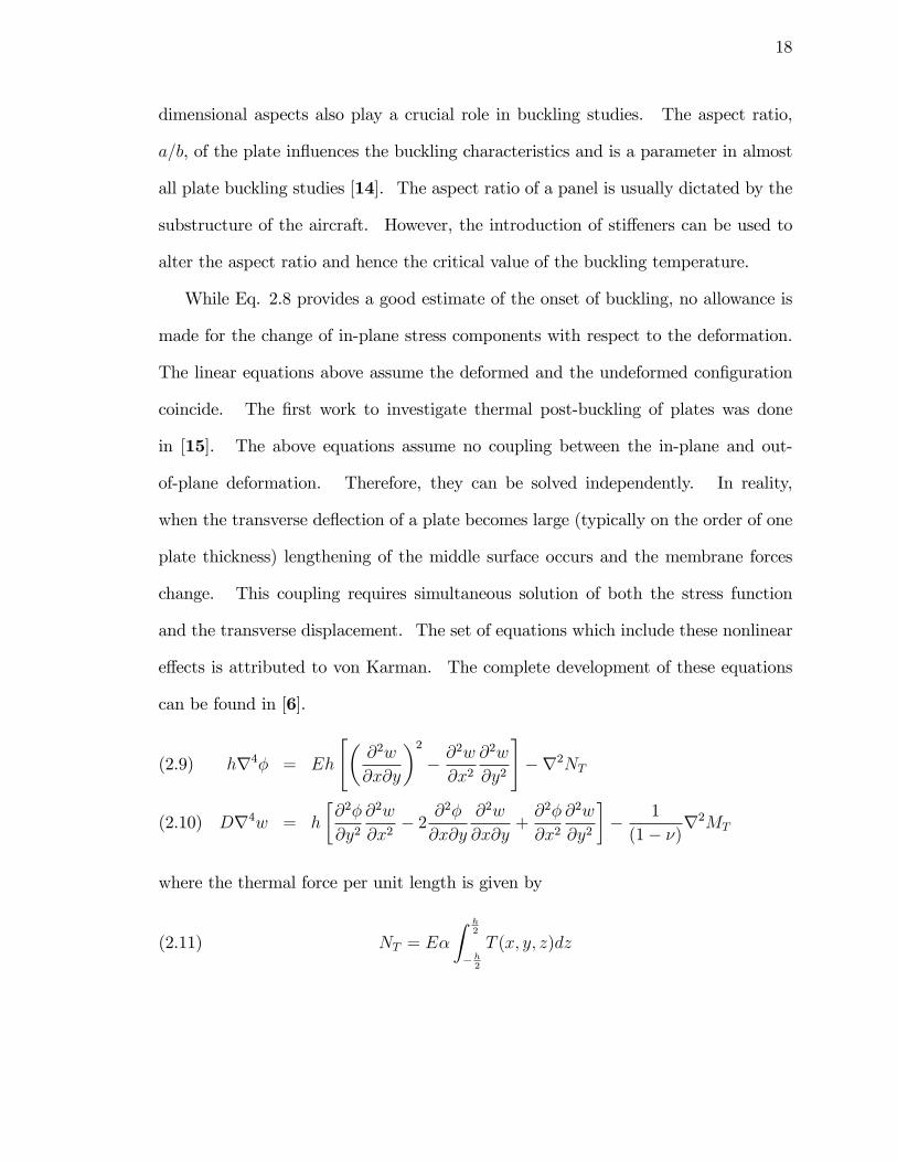
Figure 2.1 Rectangular Plate Dimensions .............................................................................16
Figure 2.2 Rectangular Plate with Edge Restraint ............................................................... 20
Figure 2.3 Spring Stiffness verses Buckling Temperature Ratio ......................................... 21
Figure 2.4 Geometry and Coordinates of a Typical Doubly-Curved Shell ......................... 22
Figure 2.5 Load Deflection Curve for Singly-Curved Shell
with Fixed Aspect Ratio and Free In-Plane Expansion ...................................... 28
Figure 2.6 Load Deflection Curve for Singly-Curved Shell
with Fixed Radius of Curvature and Free In-Plane Expansion .......................... 29
Figure 2.7 Critical Buckling Temperature Difference verses Circumferential Distance ..... 30
Figure 2.8 Load Deflection Curve for Singly-Curved Shell
with Fixed Aspect Ratio and In-Plane Restraint ..................................................32
Figure 2.9 Load Deflection Curve for Singly-Curved Shell
with Fixed Radius of Curvature and In-Plane Restraint ..................................... 32
vii
Figure 2.10 Load Deflection Curve for Singly-Curved Shell
with Fixed Curvature, Fixed Aspect Ratio, and
In-Plane Restraint .............................................................................................. 33
Figure 2.11 Unit Width Strip Beam Model .......................................................................... 35
Figure 2.12 Undeformed and Deformed Configurations of Thermally-Loaded,
Clamped-Clamped Beam ................................................................................. 36
Figure 2.13 Free-body Diagram of Deformed, Thermally-Loaded, Strip Model ................ 36
Figure 2.14 Post-buckled Configurations for Various Values of τ ...................................... 42
Figure 2.15 Maximum Mechanical Strain verses Normalized Thickness ........................... 43
Figure 2.16 Effect of Increasing Thickness on Non-dimensional Load Factor ................... 44
Figure 2.17 Undeformed and Deformed Configurations of Thermally-Loaded,
with Spring Supports ....................................................................................... 46
Figure 2.18 Buckling Temperature Ratio verses Non-dimensional Thickness
for Finite Stiffness Edge Conditions ............................................................... 47
Figure 2.19 Reaction Force Increase verses Thickness Increase for
Finite Stiffness Edge Conditions ...................................................................... 49
Figure 2.20 Moment Increase verses Thickness Increase for
Finite Stiffness Edge Conditions ...................................................................... 50
viii
Figure 2.21 Stress Ratio verses Thickness Ratio for
Finite Stiffness Edge Conditions ...................................................................... 51
Figure 2.22 Curved Beam Geometry and Reaction Forces ................................................. 53
Figure 2.23 Strain verses Non-dimensional Depth for δ/L = 0.083 ..................................... 54
Figure 2.24 Strain verses Non-dimensional Depth for δ/L = 0.042 ..................................... 54
Figure 2.25 Strain verses Non-dimensional Depth for δ/L = 0.0083 ................................... 55
Figure 2.26 Strain verses Non-dimensional Depth for δ/L = 0.0042 ................................... 56
Figure 2.27 Maximum Strain of Curved Beam verses Initial Out-of-Plane Distance ......... 56
Figure 2.28 Curved Panel Reaction Force verses Thickness for Different Values
of Initial Out-of-Plane Distance ........................................................................ 57
Figure 3.1 Variable Definitions for Homogenization Model ............................................... 63
Figure 3.2 Tip-loaded Cantilever Beam with Severe Checkerboarding Instability ............. 64
Figure 3.3 Effect of SIMP Penalty Parameter ...................................................................... 67
Figure 3.4 Minimum Compliance Example for Level Set Method ..................................... 69
Figure 3.5 Initial Design Domain Thermoelastic Topology Example ................................. 77
ix
Figure 3.6 Optimal Thermal Topology Example with ΔT = 0 ............................................ 78
Figure 3.7 Optimal Thermal Topology Example with Four-noded Elements and ΔT = 1 ...79
Figure 3.8 Optimal Thermal Topology Example with Nine-noded Elements and ΔT = 1 ...80
Figure 3.9 Optimal Thermal Topology Example with Four-noded Elements and ΔT = 4 ...81
Figure 3.10 Optimized Thickness Design for Displacement Minimization ........................ 84
Figure 3.11 Evolution History of Displacement verses Volume Ratio ............................... 84
Figure 3.12 Design Domain for a Compliant Thermal Actuator Mechanism ..................... 88
Figure 3.13 Optimized Compliant Topologies for Various Output Spring Stiffnesses ....... 89
Figure 3.14 Load and Design Domain of Thermal Snap-Fit Mechanism ............................ 89
Figure 3.15 Result for Snap-Fit Thermal Transient Actuator .............................................. 90
Figure 4.1 Initial Geometry of Curved Shell with Clamped Boundary ............................... 96
Figure 4.2 Curved Plane Stress Model of Constrained Skin ............................................... 97
Figure 4.3 Nonlinear Stress Response of Thermally-Loaded Shell with Clamped Edges .. 98
Figure 4.4 Buckling Modes of Thermally-Loaded Shell ..................................................... 99
x
Figure 4.5 Post-Buckled, Nonlinear Stress Response of Thermally-Loaded Shell
with Clamped Edges ........................................................................................ 100
Figure 4.6 Plane Strain Model of Curved Shell ................................................................. 101
Figure 4.7 Venn Diagram of Design Space Intersection Between
Axial Stress and Reaction Force ....................................................................... 102
Figure 4.8 Plane Strain Model of Curved Shell with Enforced Boundary Condition ....... 103
Figure 4.9 Axial Stress verses Out-of-Plane Displacement for Plane Model .................... 104
Figure 4.10 Reaction Force verses Out-of-Plane Displacement for Plane Model ............ 105
Figure 4.11 Reaction Force verses Out-of-Plane Displacement for Plane Model ............ 106
Figure 4.12 Curved Shell with Conventional Stiffening ................................................... 107
Figure 4.13 Initial Design Domain Featuring Fixed and Designable Regions .................. 107
Figure 4.14 Minimum Compliance Topology Design for Thermal Load
of 900ºF and 15% Volume Constraint ............................................................ 108
Figure 4.15 Minimum Compliance Topology Design for Thermal Load
of 900ºF and 30% Volume Constraint ............................................................ 108
Figure 4.16 Initial Design Domain with Mechanical Loads .............................................. 109
Figure 4.17 Stiffener Generated from Mechanical Loading
xi
with 30% Volume Constraint ......................................................................... 110
Figure 4.18 Stiffener Generated from Mechanical Loading
with 15% Volume Constraint ......................................................................... 110
Figure 4.19 Reaction Force Comparisons for Thermally and Mechanically
Derived Stiffeners ........................................................................................... 111
Figure 4.20 Reaction Moment Comparisons for Thermally and Mechanically
Derived Stiffeners ........................................................................................... 111
Figure 4.21 Deformed and Undeformed Configurations for
Mechanically-Derived Stiffener ..................................................................... 112
Figure 4.22 Principal Stress Contours for Mechanically-Derived
Stiffener/Skin Combination ............................................................................ 113
Figure 5.1 An Initial Metallic Thermal Protection System .................................................129
Figure 5.2 Relationship Between Fundamental Frequency and Maximum Stress ............ 131
Figure 5.3 Evolutionary Histories of the Fundamental Frequencies
and Maximum Thermal Stress .......................................................................... 135
Figure 5.4 Resultant TPS Models with 900 Hz Natural Frequency .................................. 138
Figure 5.5 Initial Model for Design of TPS Support ......................................................... 140
xii
Figure 5.6 Evolutionary Histories for TPS Support Design .............................................. 141
Figure 5.7 Optimum TPS Support ..................................................................................... 142
Figure 5.8 Evolutionary History of Fundamental Frequency for TPS Frame ................... 143
Figure 5.9 Optimum TPS Model Including Heat Transfer Effects .................................... 145
xiii
Acknowledgments
I would like to take this opportunity to thank all the people who have given up so
much to allow me the opportunity to fulfill my dreams. First and foremost, I want to thank
my wife Jennifer who has been there to support me in every way possible. She has kept our
family running the last few years while “Daddy was busy.” I will spend the rest of my life
making up for the sacrifices she has made. To my two children, Taylor and Sara, thank you
for understanding when Dad couldn't give you all the time you deserved and for the many
times you both cut the grass so Dad could work. I want to thank my father, Terry, for being
an incredible inspiration to me. Anyone who has pursued an advanced degree in engineering
has, at some point, entertained the thought of quitting. When these thoughts entered my
mind, my father's example of toughness and persistence have given me the strength to
persevere. Thanks also to my mother, Margaret, for all the years of unconditional love and
support. I would also like to thank my father and mother-in-law, Bill and Paula, for their
love and faith in me.
A special thanks must be given to my advisor, Dr. Ramana Grandhi. Dr. Grandhi has
demonstrated great patience over the last three years in accommodating my busy work
schedule at the Air Force Research Lab. I want to thank him especially for his encouraging
words that have, on many occasions, reassured me that I am “Ph.D. Material.” As a world-
renown researcher, Dr. Grandhi has afforded me, as well as his other students, opportunities
that do not exist but to an elite few. The opportunity to publish with Dr. Grandhi has been
xiv
one of my proudest achievements and I look forward to continuing the tradition of high
quality publications as a product of Dr. Grandhi's research circle. Thanks are also extended
to my co-advisor, Dr. Ravinder Chona. Dr. Chona, as the leader of the Structural Sciences
Center of the Air Force Research Lab, has constantly provided me excellent career advice as
well as encouragement throughout this endeavor. His greetings of “Dr. Haney” have been
an affirmation of his belief in my ability and I look forward to years of service in the
Structural Sciences Center, under Dr. Chona, as we produce the technologies that will enable
the U.S. Air Force to meet the challenges of the future. I would also like to thank the other
members of my committee, Drs. Penmetsa, Cornelius and Thompson for their participation
in the Ph.D. candidacy process as well as the review of this manuscript. Having been
involved in several Masters students' theses, I appreciate the commitment made by all the
members of my committee.
I now want to take this opportunity to thank the Air Force Research Lab Air Vehicles
Directorate and in particular the Structures Division for their commitment to this process. I
would never have been able to accomplish this task without being given the time by my
management to focus almost solely on this work. Dr. Kristina Langer, Chief of the
Analytical Structural Mechanics Branch, has played a very important role in my success at
AFRL. Dr. Langer was first to involve the Structures Division in the root cause analysis of
the B-2 aft deck. I am thankful that I was chosen as a member of that award-winning team
as that difficult problem became the inspiration for much of this work. Dr. Langer has been
xv

a good friend to me and has given me countless encouraging words along with any tool
needed to complete this work. She never hesitated in pulling whatever strings were needed
to assure that I had adequate time to achieve this goal. I also want to take this opportunity to
thank Mr. Michael Camden. Mike served as the technical leader in thermal structures for
several years in the Structures Division. I had the great opportunity of working with Mike
and having him serve as my mentor over the past two years. Mike has been a constant
source of encouragement to me and without his initiative, I would not have completed this
work. Mike petitioned our management to pay more than lip service to the time
commitment necessary for this undertaking. He was successful and I am the benefactor. I
also want to thank Mr. John Bowlus, Chief of the Structures Division. As many who know
me are aware, my personality rarely allows me to say “no” when presented with exciting
work. Mr. Bowlus took on this responsibility for me. He reassigned people to take on my
other responsibilities and supported me in countless other ways. I would also like to thank
AFRL/VAS Division for providing my salary as I completed this work.
I want to acknowledge a few of my co-workers who have contributed to this work by
being excellent sounding boards for my ideas. In particular, I want to thank Dr. Thomas
Eason for his advice and encouragement over the past year. Special thanks also goes to Mr.
Brett Hauber who has provided many insights into thermal structures from his propulsion
perspective. I would also like to thank Dr. Steven Spottswood for our interesting
conversations and for his willingness to provide insights into acoustic response of structures.
xvi

I also want to thank Dr. Anthony Ingraffea of Cornell University for his career advice and
for the rounds of golf that provided a much needed distraction. Thanks also goes to Dr.
Joseph Hollkamp for our discussions of panel buckling and dynamic response. I would also
like to express my appreciation to Mr. Robert Gordon for his many insights into dynamic
and acoustic response of thin panels. And lastly, I want to thank Dr. Larry Byrd. Larry has
been a great friend for the last 17 years. So many of the world's problems have been solved
on our lunchtime walks. Larry has seen me through the lows and highs of the Ph.D. Process.
He has taught me patience and endurance. About three years ago, Larry faced a debilitating
disease which left much of this body paralyzed. I visited Larry in the hospital and witnessed
his relentless fight to recover. When he could only move his arms, he moved them
continuously. He refused to surrender to the effects of this disease. Larry's struggle and
subsequent victory over this condition have been a tremendous source of encouragement to
me and have given me strength. Larry recently shared with me a quote from The Alchemist,
“if you pursue your dreams, the whole universe conspires in helping you achieve it.”[1]
There is no better quote to sum up the experiences of my life.
xvii
CHAPTER 1
Introduction
1.1. Motivation
The age-old adage "necessity is the mother of invention" is appropriate in describ-
ing the genesis of this work. Over the past three years the author along with other
members of the Air Force Research Lab Structures Division (AFRL/VA) have been
involved in the root cause investigation of premature cracking of the aft deck of the
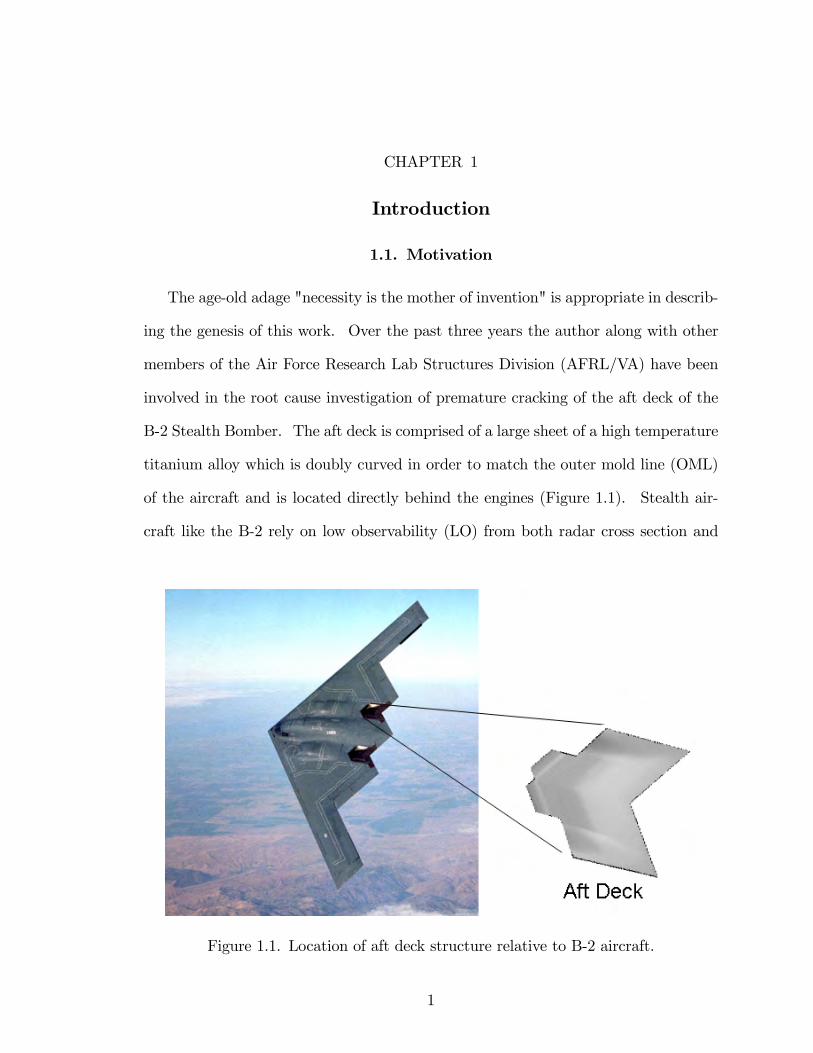
B-2 Stealth Bomber. The aft deck is comprised of a large sheet of a high temperature
titanium alloy which is doubly curved in order to match the outer mold line (OML)
of the aircraft and is located directly behind the engines (Figure 1.1). Stealth air-
craft like the B-2 rely on low observability (LO) from both radar cross section and
Figure 1.1. Location of aft deck structure relative to B-2 aircraft.
1
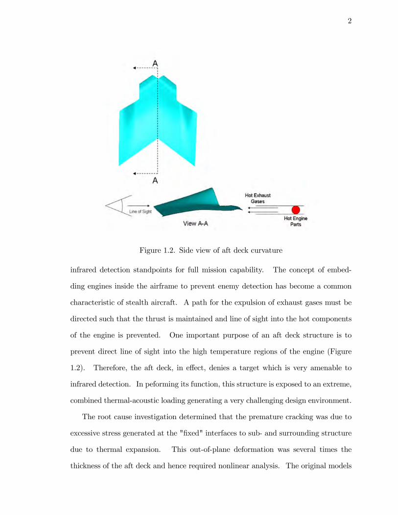
2
Figure 1.2. Side view of aft deck curvature
infrared detection standpoints for full mission capability. The concept of embed-
ding engines inside the airframe to prevent enemy detection has become a common
characteristic of stealth aircraft. A path for the expulsion of exhaust gases must be
directed such that the thrust is maintained and line of sight into the hot components
of the engine is prevented. One important purpose of an aft deck structure is to
prevent direct line of sight into the high temperature regions of the engine (Figure
1.2). Therefore, the aft deck, in e¤ect, denies a target which is very amenable to
infrared detection. In peforming its function, this structure is exposed to an extreme,
combined thermal-acoustic loading generating a very challenging design environment.
The root cause investigation determined that the premature cracking was due to
excessive stress generated at the "�xed" interfaces to sub- and surrounding structure
due to thermal expansion. This out-of-plane deformation was several times the
thickness of the aft deck and hence required nonlinear analysis. The original models
3
were analyzed using MSC/Nastran linear static analysis and therefore did not predict
the failure condition. As cracks formed and grew to appreciable lengths, the natural
frequency of the structure decreased. With wide-band random noise impinging on
the structure from the engine exhaust, this frequency drop resulted in additional high
cycle fatigue damage which accelerated the crack growth rate.
The traditional approach to the design of thermal structures typically includes
a prescription for allowing thermal expansion. Thermal stresses result when this
expansion is inhibited. Aerospace examples of this approach to hot structures can
be found in engine liners, tailpipes and the well-known example of the fuel system
of the SR-71 [1]. This concept is not, however, unique to the aerospace industry as
very familiar examples are found in expansion joints in concrete sections and in the
slotted attachment of vinyl siding for home exterior.
An approach that allowed for thermal expansion was investigated for the long-
term solution of the engine exhaust-washed structure (EEWS) of the B-2. There were
several considerations that made this solution unworkable. Firstly, the aft deck, while
not being in the primary �ight load path, does, in fact, carry a small but signi�cant
share of the �ight loads. Removing the attachment to surrounding structure and
implementing a "�oating" design which was free to expand would, indeed, reduce the
aft deck thermal stress; however, �ight load would be reacted in structure not designed
for this purpose. Secondly, a concern was raised with respect to an increase in radar
cross section. An expansion joint would introduce a discontinuity in the outer mold
line of the aircraft and could potentially impact the mission capability of the plane.
A cover seal that is used at other junctures of the plane to conceal stationary gaps was
investigated as a potential solution. These knife-edge seals (Figure 1.3) were found
to be inadequate for a sliding interface due to potential curling of the edges resulting
from the stick-slip nature of frictional contact. A cavity similar to that shown in
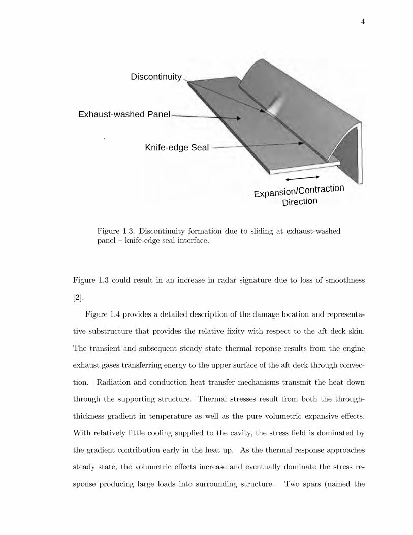
4
Knifeedge Seal
Expansion/Contraction
Direction
Exhaustwashed Panel
Discontinuity
Knifeedge Seal
Expansion/Contraction
Direction
Exhaustwashed Panel
Discontinuity
Figure 1.3. Discontinuity formation due to sliding at exhaust-washedpanel �knife-edge seal interface.
Figure 1.3 could result in an increase in radar signature due to loss of smoothness
[2].
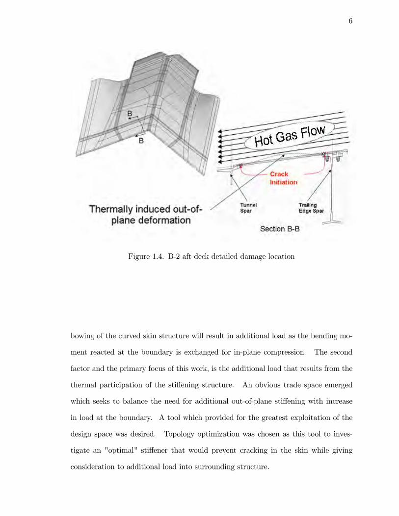
Figure 1.4 provides a detailed description of the damage location and representa-
tive substructure that provides the relative �xity with respect to the aft deck skin.
The transient and subsequent steady state thermal reponse results from the engine
exhaust gases transferring energy to the upper surface of the aft deck through convec-
tion. Radiation and conduction heat transfer mechanisms transmit the heat down
through the supporting structure. Thermal stresses result from both the through-
thickness gradient in temperature as well as the pure volumetric expansive e¤ects.
With relatively little cooling supplied to the cavity, the stress �eld is dominated by
the gradient contribution early in the heat up. As the thermal response approaches
steady state, the volumetric e¤ects increase and eventually dominate the stress re-
sponse producing large loads into surrounding structure. Two spars (named the
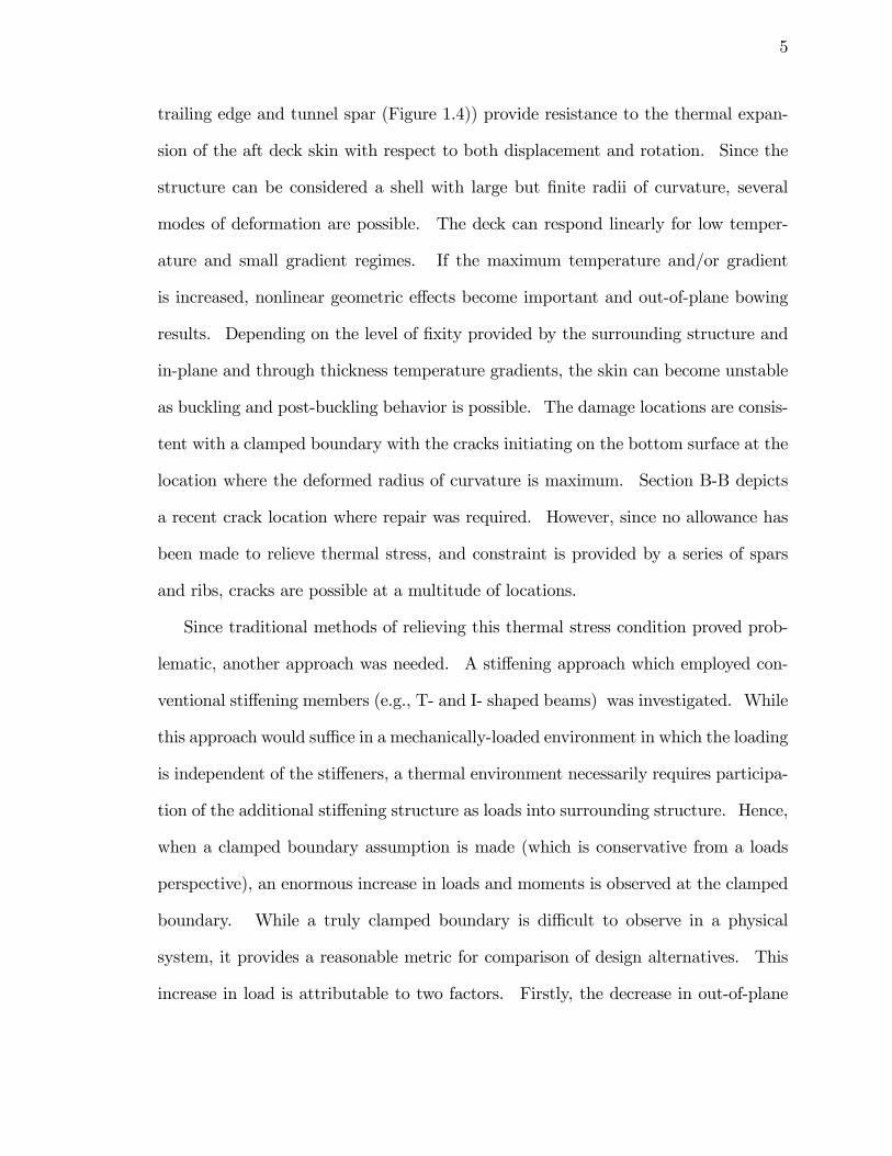
5
trailing edge and tunnel spar (Figure 1.4)) provide resistance to the thermal expan-
sion of the aft deck skin with respect to both displacement and rotation. Since the
structure can be considered a shell with large but �nite radii of curvature, several
modes of deformation are possible. The deck can respond linearly for low temper-
ature and small gradient regimes. If the maximum temperature and/or gradient
is increased, nonlinear geometric e¤ects become important and out-of-plane bowing
results. Depending on the level of �xity provided by the surrounding structure and
in-plane and through thickness temperature gradients, the skin can become unstable
as buckling and post-buckling behavior is possible. The damage locations are consis-
tent with a clamped boundary with the cracks initiating on the bottom surface at the
location where the deformed radius of curvature is maximum. Section B-B depicts
a recent crack location where repair was required. However, since no allowance has
been made to relieve thermal stress, and constraint is provided by a series of spars
and ribs, cracks are possible at a multitude of locations.
Since traditional methods of relieving this thermal stress condition proved prob-
lematic, another approach was needed. A sti¤ening approach which employed con-
ventional sti¤ening members (e.g., T- and I- shaped beams) was investigated. While
this approach would su¢ ce in a mechanically-loaded environment in which the loading
is independent of the sti¤eners, a thermal environment necessarily requires participa-
tion of the additional sti¤ening structure as loads into surrounding structure. Hence,
when a clamped boundary assumption is made (which is conservative from a loads
perspective), an enormous increase in loads and moments is observed at the clamped
boundary. While a truly clamped boundary is di¢ cult to observe in a physical
system, it provides a reasonable metric for comparison of design alternatives. This
increase in load is attributable to two factors. Firstly, the decrease in out-of-plane
6
Figure 1.4. B-2 aft deck detailed damage location
bowing of the curved skin structure will result in additional load as the bending mo-
ment reacted at the boundary is exchanged for in-plane compression. The second
factor and the primary focus of this work, is the additional load that results from the
thermal participation of the sti¤ening structure. An obvious trade space emerged
which seeks to balance the need for additional out-of-plane sti¤ening with increase
in load at the boundary. A tool which provided for the greatest exploitation of the
design space was desired. Topology optimization was chosen as this tool to inves-
tigate an "optimal" sti¤ener that would prevent cracking in the skin while giving
consideration to additional load into surrounding structure.
7
1.2. Research Objectives
It should be emphasized that while a recent failure investigation provided the
motivation for this work, the implications are much broader. When possible, tradi-
tional methods of alleviating thermal stress should be employed, namely, permitting
the expansion to take place. For example in the B-2 aft deck investigation, in the
regions where damage was observed initially, the stresses could be practically elimi-
nated if a few hundreths of an inch expansion were permitted over length scales of 10
to 12 inches. However, any situation which does not permit the alleviation of ther-
mal stress by expansion can bene�t from the concepts revealed in this dissertation.
Hence, future stealth aircraft with embedded engines will undoubtable encounter si-
miliar design di¢ culties. Therefore, this work addresses a class of problems where
design solutions will continue to be extremely important to the long-term vision of
the Air Force. Since the exact geometry of future aircraft will di¤er from that en-
countered on the B-2, without loss of generality, simple, single-curved shells and beam
strips are used in this work to demonstrate the salient features of the tools developed
in this dissertation.
The research objectives in this work are threefold. The �rst is to identify the
non-intuitive nature of the problem being addressed. Examples will be presented
which demonstrate how the structural analyst, who is familiar with the design of
mechanically-loaded structures, must use extreme caution when applying this "room
temperature" mentality to constrained thermal structures. Secondly, well-established
topology methods will be utilized to evolve a structure which balances the two objec-
tives of stress reduction in the skin and load into surrounding strucuture by taking
advantage of a de�ciency in the classical, minimum compliance topology optimization
formulation. And lastly, a novel evolutionary structural optimization (ESO) method
is developed which simultaneously addresses von-Mises stress and frequency for the
8
more general application of thermal protection systems. Since the environment under
consideration contains acoustic as well as thermal energy, maintaining fundamental
frequency at high levels reduces the potential damage from acoustic loading.
1.3. Chapter Outline
This work begins with a review of previous e¤orts relevant to this development.
Chapter 2 is a review of thermal structures relevant to this development. Since
plane stress shells are used to model the skin response and are the focus of the failure
location, the thermal structures chapter provides a literature review which includes
a survey of previous work in thermally loaded shell geometries. The nature of the
di¢ culty in sti¤ening thermally loaded structures is illustrated by a series of sim-
ple, but revealing, examples. These results provide additional motivation for the
current work as well as demonstrating the necessity of advanced analysis and opti-
mization tools for robust designs in this environment. With topology optimization
being a primary focus of this work, Chapter 3 is devoted to providing an historical
perspective of this subject beginning with the discrete nature of the problem and the
mathematical ill-posedness of the formulation. Relaxation methods such as homog-
enization and the widely used SIMP (Simple Isotropic Material with Penalization)
are introduced to overcome the di¢ culties associated with �0-1�nature of the integer
programming problem. A less mathematically rigorous topology formulation known
as evolutionary structural optimization (ESO) is then introduced which does address
the discrete problem directly through a slow process of �nite element removal. The
ESO method provides the framework for the topology formulation in Chapter 4 which
simultaneously treats thermal stress and fundamental frequency. And lastly, a rela-
tive new-comer to the world of topology optimization formulations is brie�y discussed
in the Level-Set method.
9
Topology optimization began as a tool exclusively applied to solid mechanics.
Since that time, many formulations have evolved which apply topology optimization
to the energy equation [3], Stoke�s �ow [4], and multi-physics applications [5]. In this
work, the focus is exclusive to solid mechanics so the review provided begins with the
minimum compliance formulation for mechanically-loaded structures and eventually
narrows the focus to nonlinear thermoelasticity.
In Chapter 4, conventional minimum compliance topology optimization is applied
to the sti¤ening of a thin, shallow shell geometry in an elevated temperature environ-
ment by taking advantage of a known de�ciency in topology optimization associated
with single load case mechanical loadings. A novel multi-objective ESO topology
method which seeks to minimize thermal stress while simultaneously increasing the
fundamental frequency of a thermal protection system (TPS) panel is developed in
Chapter 5. Chapter 5 provides paths for future work including a formulation which
directly addresses the reaction force vs out-of-plane deformation trade space.
CHAPTER 2
Thermal Structures Review
2.1. Historical Perspective
When one begins a study of thermal structures and thermal stress response, two
classic texts on the topic should be thoroughly reviewed. The �rst, Boley and Weiner
[6], provides a very rigorous mathematical treatment of the subject matter for linear
thermoelasticity. The coupled treatment of both the energy equation and elastic
equilibrium is developed. Guidelines for when the equations must be solved in a
coupled fashion and when a sequential, weak coupling of the thermal and structural
solutions is adequate are presented. Linear buckling of plates is addressed and solu-
tions for various boundary conditions are provided. The inclusion of nonlinear strain
coupling between the membrane and bending e¤ects is developed and an analytical
solution is provided for the unrestrained condition. Many of the analytical solutions
presented in [6] examine the unconstrained case in which stresses result from in-plane
and through-thickness temperature gradients. The stresses generated from this type
of loading are, in practice, smaller than those observed when overall volumetric ex-
pansion of prevented, i.e., clamped boundaries, except in the case of thermal shock
where very localized heating takes place.
The second text, which has a slightly more applied �avor, in particular, to the
aerospace industry, is the text by Gatewood [7]. Analytical and semi-analytical
solutions are presented for skin-stringer combinations and other familiar aerospace
constructs. Common to both references is the treatment of both transient and
steady state e¤ects. Gatewood provides a more thorough treatment of temperature
10
11
dependent material properties which over large temperature ranges, can be quite
pronounced and if neglected can lead to misleading results.
The impetus for our ability to simulate the response of structures to thermal
loading began in the early 1950�s with the breaking of the sound barrier in the X-
1A experimental aircraft program. Compressible gas dynamics predicts that large
temperature increases can accompany frictional e¤ects from the conversion of kinetic
energy in the �owstream to internal energy (in the form of heat) at the �uid-structure
interface. The generated heat �ux inpinges on the surface of the vehicle and causes an
accompanying temperature increase. The second mechanism associated with super-
sonic �ight which can potentially generate very high temperatures in localized areas
is that of shock wave generation. Shocks are typically produced when supersonic
�ow is reduced to subsonic �ow at a point of stagnation such as a leading edge of a
wing or other control surface on the vehicle. The �rst vehicle on which aerothermal
heating was studied was the X-1B [8]. The X-1B was a more sophisticated version
of Captain Charles E. Yeager�s initial supersonic vehicle. Mach numbers reached by
the X-1B were just under Mach 2. The aerodynamic heating e¤ects for the given air
velocity and altitude resulted in skin temperatures of approximately 2000F . Con-
ventional aluminum airframes were capable of surviving this environment, however,
higher temperature material systems would be vital to enable higher speed vehicles.
As technology advanced in propulsion systems, supersonic speeds increased rapidly,
and aerodynamic heating e¤ects began to dominate the designs. The challenges of
managing the thermal environment and the associated di¢ culties became known as
the thermal barrier [1].
The X-2 was the �rst aircraft designed in which aerodynamic heating e¤ects were
given full consideration [9]. Up to this point, speeds had not been large enough for
aerodynamic heating to adversely a¤ect the aircraft performance. In 1956, the X-2
12
achieved a Mach number of 2.5. This capability was realized through high temper-
ature material systems. The fuselage was constructed from K-Monel with the skins
consisting of stainless steel. These heavier materials systems were a penalty from
a payload and performance perspective when compared with aluminum. However,
they were an enabling component of high speed �ight. This trade-o¤ between pay-
load and thermal protection continues to be an important trade space. These e¤orts
are well documented in [10].
The next signi�cant achievement in the realm of thermal structures occured with
the establishment of the X-15 program. One of the many X planes that furthered
American aviation supremacy, the X-15 consisted of a thick-skinned vehicle made of
high temperature, nickel-based alloys (Inconel-X). The �ights were short in duration
typically lasting from 10 to 12 minutes [11]. The maximum temperature reached on
the vehicle occured at one of the primary stagnation points (the wing leading edges)
and exceeded 13000F . One of the principal events of the twentieth century with re-
spect to the so-called race to space was the success of the Sputnik I program After
the Soviets successfully orbited the world�s �rst man-made satellite (Sputnik I), the
X-15 program became a very important national priority with regard to the unde-
standing of aerothermal structures. The X-15 made many signi�cant contributions
to the understanding of hypersonic �ight including the design of thermal structures.
The success of Sputnik forced United States hypersonic �ight research to change
focus and to make space access its number one priority. Along with this change
of focus, came an even more challenging thermal-structural environment. With
Mach numbers approaching twenty, the maximum temperatures predicted on the
lifting bodies were in excess of 30000F . Two approaches were taken to mitigate this
extreme environment. The cool structures approach sought to insulate the primary
load bearing structure from the intense heat by means of a thermal shield. These
13
barriers were made of high temperature metals, ceramic or ablative material and
carried virtually no �ight load. Hence, their weight was parasitic, penalizing the
mission payload. These type of systems are designed for transient thermal loads
that are associated with re-entry. The insulation layer is designed such that the
low-temperature airframe never reaches some speci�ed critical temperature. If no
active cooling is provided, these structures cannot operate at a steady state condtion
as the backing structure would eventually reach a temperature above its usage. This
cool structures approach has been somewhat successfully demonstrated on the space
shuttle, but the fragililty of the thermal protection system (TPS) has resulted in
costly losses including loss of life in the case of the Columbia tragedy.
An alternative approach to successful operation in the elevated temperature envi-
ronment is often referred to as hot structures. Hot structures are designed to operate
at or near the skin temperature. Hot structures are intended to participate in the
load path reaction and are integral to the airframe. The obvious advantage of hot
structure is that its weight is non-parasitic. This bene�t can potentially reduce the
cost to achieve lower earth orbit (LEO) with a payload. The challenges associated
with this approach make this area an active research �eld. The material systems
that can tolerate the high temperature environment are inherently brittle and have
low damage tolerance. Therefore, to use these materials as load carrying structure
is extremely challenging. The material science community has attempted to incor-
porate acceptable damage tolerance characteristics into ceramic-like material systems
by resorting to high-temperature composites. The combination of ceramic �bers with
a damage tolerant matrix has generated some success. Another approach to mitigat-
ing the risk associated with these materials is to employ structural health monitoring
(SHM). Since small cracks in brittle materials can cause catastrophic failure, embed-
ded sensors to detect damage before it becomes critical are being pursued to mitigate
14
this risk. SHM is an active area of research and is one of the primary foci of research
funding of the Department of Defense and the Air Force Research Lab.
Engine exhaust-washed structures can be categorized as hot structure given that
they are exposed directly to a high temperature environment absent a thermal barrier
coating or insulation. Since the EEWS is expected to operate continuously for long
periods of time, a low-conductivity coating would only succeed in smoothing out the
early transients and delaying the heat transfer through the thickness. After a period
of time, the skin EEWS would come up to temperature as steady state conditions
dominate. While much of the work in hot structures assumes the high temperature
environment is a result of aerodynamic heating and Chapter 5 of this work examines
this case, an additional high temperature environment exists due to exhaust wash from
embedded engines in low-observable aircraft. And hence, the structure is exposed to
overall sound pressure levels (OSPL) that can potentially result in acoustic excitation
and additional damage accumulation.
2.2. Plates and Shells
Since the structure considered here can best be idealized as a shell, [12] is useful
in studying the past work in themal-mechancial response of plate and shell struc-
tures. Plates and shells exposed to thermal energy can respond in several di¤erent
ways depending on the in-plane temperature variation, through-thickness temperature
gradient, and essential boundary conditions. Depending on these inputs, the panel
may continuously deform out-of-plane (bowing); however, under appropriate condi-
tions, buckling and subsequent post-buckling response does occur. When studying
�at plates subjected to thermal loading, buckling is the primary response and occurs
at relatively low temperatures. As initial curvature is introduced into the geometry,
a shell geometry results and the buckling temperature increases [12]. This result
15
is intuitive as buckling occurs due to instability which forces the structure to follow
bifurcated equlibrium paths. If the structure contains intial curvature, a smooth equi-
librium path may exist independent of buckling which allows for thermal expansion
albeit out-of-plane.
2.2.1. Flat Plate Response
Plates and shells can be categorized more broadly as plane stress structural elements.
In plane stress, the deformation is assumed to be a function of the in-plane coordinates
only. As the name implies, a plane state of stress exists such that the transverse
components of stress are assumed to be zero. Plane stress is identi�ed with thin sheets
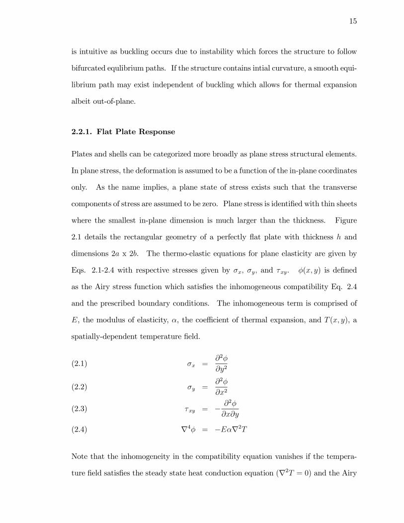
where the smallest in-plane dimension is much larger than the thickness. Figure
2.1 details the rectangular geometry of a perfectly �at plate with thickness h and
dimensions 2a x 2b. The thermo-elastic equations for plane elasticity are given by
Eqs. 2.1-2.4 with respective stresses given by �x; �y; and �xy. �(x; y) is de�ned
as the Airy stress function which satis�es the inhomogeneous compatibility Eq. 2.4
and the prescribed boundary conditions. The inhomogeneous term is comprised of
E, the modulus of elasticity, �, the coe¢ cient of thermal expansion, and T (x; y), a
spatially-dependent temperature �eld.
�x =@2�
@y2(2.1)
�y =@2�
@x2(2.2)
�xy = � @2�
@x@y(2.3)
r4� = �E�r2T(2.4)
Note that the inhomogeneity in the compatibility equation vanishes if the tempera-
ture �eld satis�es the steady state heat conduction equation (r2T = 0) and the Airy
16
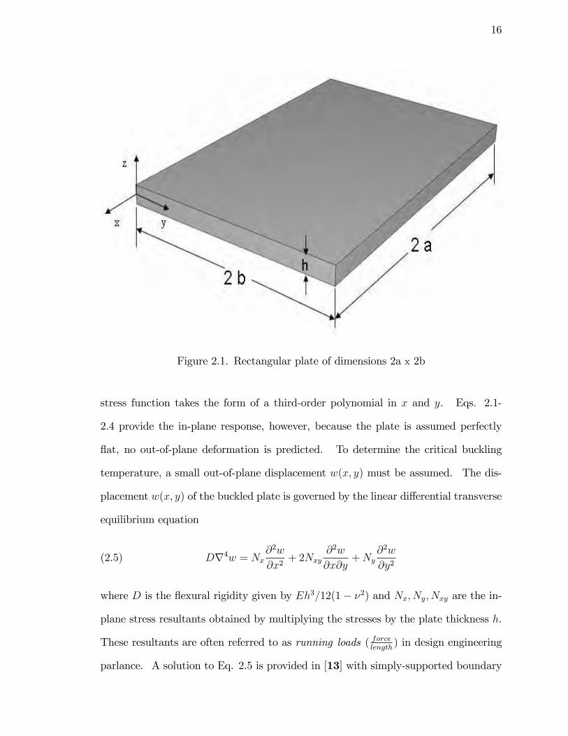
Figure 2.1. Rectangular plate of dimensions 2a x 2b
stress function takes the form of a third-order polynomial in x and y. Eqs. 2.1-
2.4 provide the in-plane response, however, because the plate is assumed perfectly
�at, no out-of-plane deformation is predicted. To determine the critical buckling
temperature, a small out-of-plane displacement w(x; y) must be assumed. The dis-
placement w(x; y) of the buckled plate is governed by the linear di¤erential transverse
equilibrium equation
(2.5) Dr4w = Nx@2w
@x2+ 2Nxy
@2w
@x@y+Ny
@2w
@y2
where D is the �exural rigidity given by Eh3=12(1� �2) and Nx; Ny; Nxy are the in-
plane stress resultants obtained by multiplying the stresses by the plate thickness h.
These resultants are often referred to as running loads ( forcelength
) in design engineering
parlance. A solution to Eq. 2.5 is provided in [13] with simply-supported boundary
17
conditions and is given by
(2.6) Nxm2�2
(2a)2+Ny
n2�2
(2b)2= D
�m2�2
(2a)2+n2�2
(2b)2
�2where m and n represent the number of waves in the x and y directions, respectively.
For a 2a x 2b �at plate, the in-plane running loads for the uniform thermal loading,
�T , are given by
(2.7) Nx = Ny =� �T E h
(1� �)
Substituting these force expressions into Eq. 2.6 along with the expression for D, and
using the minimum values of m and n (=1), the critical buckling temperature change
is given by
(2.8) �Tcr =�2h2
48(1 + �)�(1
a2+1
b2)
One important conclusion drawn from Eq. 2.8 is the independence of modulus of
elasticity. This is unique to thermal buckling as buckling caused by mechanical
loading is a function of material sti¤ness [13]. Eq. 2.8 predicts extremely small
buckling temperature changes. For example, an aluminum plate with a = 18 in,
b = 12 in, and h = 0:25 in with � = 13:0 � in/in��F buckles at a temperature
change above room temperature of 7.5�F . The most obvious parameter to increase if
thermal buckling is a concern is the thickness. This quadratic dependence increases
the buckling temperature by a factor four each time the thickness is doubled. Also
note that the buckling dependence is inversely proportional the coe¢ cient of thermal
expansion (CTE). Therefore, if several materials are being considered for a high
temperature application, the material with the lowest CTE should be chosen provided
the material properties remain stable at the desired operational temperature. The
18
dimensional aspects also play a crucial role in buckling studies. The aspect ratio,
a=b, of the plate in�uences the buckling characteristics and is a parameter in almost
all plate buckling studies [14]. The aspect ratio of a panel is usually dictated by the
substructure of the aircraft. However, the introduction of sti¤eners can be used to
alter the aspect ratio and hence the critical value of the buckling temperature.
While Eq. 2.8 provides a good estimate of the onset of buckling, no allowance is
made for the change of in-plane stress components with respect to the deformation.
The linear equations above assume the deformed and the undeformed con�guration
coincide. The �rst work to investigate thermal post-buckling of plates was done
in [15]. The above equations assume no coupling between the in-plane and out-
of-plane deformation. Therefore, they can be solved independently. In reality,
when the transverse de�ection of a plate becomes large (typically on the order of one
plate thickness) lengthening of the middle surface occurs and the membrane forces
change. This coupling requires simultaneous solution of both the stress function
and the transverse displacement. The set of equations which include these nonlinear
e¤ects is attributed to von Karman. The complete development of these equations
can be found in [6].
hr4� = Eh
"�@2w
@x@y
�2� @
2w
@x2@2w
@y2
#�r2NT(2.9)
Dr4w = h
�@2�
@y2@2w
@x2� 2 @
2�
@x@y
@2w
@x@y+@2�
@x2@2w
@y2
�� 1
(1� �)r2MT(2.10)
where the thermal force per unit length is given by
(2.11) NT = E�
Z h2
�h2
T (x; y; z)dz

19
and the thermal moment per unit length is given by
(2.12) MT = E�
Z h2
�h2
T (x; y; z)zdz
Insight may be gained into Eqs. 2.11-2.12 by considering a temperature �eld inde-
pendent of the normal coordinate z. Being an even function, the thermal force has
a contribution to the solution, whereas, the thermal moment vanishes identically.
While the boundary conditions are not explicity stated in the above formulation, it is
understood that the functions � and w, must satisfy the prescribed essential and/or
natural boundary conditions. Most thermal stress problems of interest are associated
with constraint of the expansion, in fact, for a steady state temperature �eld in an
isotropic body with an unconstrained boundary, no thermal stress exists [7]. This,
however, does not hold true for arbritary temperature �elds.
2.2.2. Simply-Supported Finite Sti¤ness Boundary
Because thermal stress is a function of restrained thermal expansion, the thermoelastic
response is highly dependent on the boundary conditions. As was stated previously,
for certain temperature distributions, the thermal stress response is zero if the body
is unconstrained. As the level of constraint is increased, the potential for higher
stresses and larger reaction loads into surrounding structure exists. An investigation
of the e¤ects of varying boundary sti¤nesses on thermally loaded, simple-supported
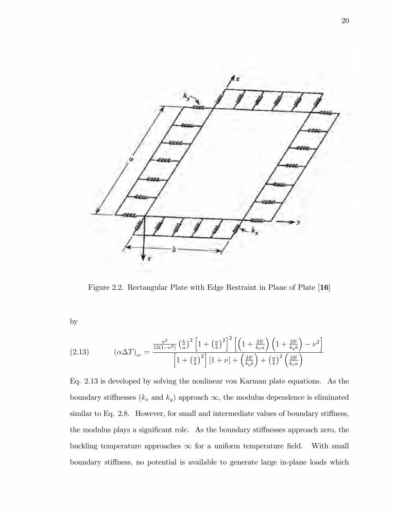
�at plates was conducted in [16]. Figure 2.2 illustrates the boundary sti¤nesses in the
x and y directions supporting a �at plate in the plane. For a �at plate, elastic tensile
stresses capable of producing failure can only be generated if panel buckling occurs.
The critical buckling temperature which incorporates the boundary sti¤nesses is given
20
Figure 2.2. Rectangular Plate with Edge Restraint in Plane of Plate [16]
by
(2.13) (��T )cr =
�2
12(1��2)�ha
�2 h1 +
�ab
�2i2 h�1 + 2E
kxa
��1 + 2E
kyb
�� �2
ih1 +
�ab
�2i[1 + �] +
�2Ekyb
�+�ab
�2 � 2Ekxa
�Eq. 2.13 is developed by solving the nonlinear von Karman plate equations. As the
boundary sti¤nesses (kx and ky) approach 1; the modulus dependence is eliminated
similar to Eq. 2.8. However, for small and intermediate values of boundary sti¤ness,
the modulus plays a signi�cant role. As the boundary sti¤nesses approach zero, the
buckling temperature approaches 1 for a uniform temperature �eld. With small
boundary sti¤ness, no potential is available to generate large in-plane loads which
21
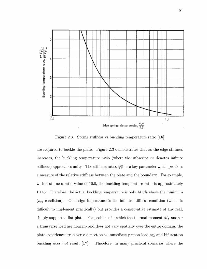
Figure 2.3. Spring sti¤ness vs buckling temperature ratio [16]
are required to buckle the plate. Figure 2.3 demonstrates that as the edge sti¤ness
increases, the buckling temperature ratio (where the subscript 1 denotes in�nite
sti¤ness) approaches unity. The sti¤ness ratio, kxa2E, is a key parameter which provides
a measure of the relative sti¤ness between the plate and the boundary. For example,
with a sti¤ness ratio value of 10.0, the buckling temperature ratio is approximately
1.145. Therefore, the actual buckling temperature is only 14.5% above the minimum
(k1 condition). Of design importance is the in�nite sti¤ness condition (which is
di¢ cult to implement practically) but provides a conservative estimate of any real,
simply-supported �at plate. For problems in which the thermal moment MT and/or
a transverse load are nonzero and does not vary spatially over the entire domain, the
plate experiences transverse de�ection w immediately upon loading, and bifurcation
buckling does not result [17]. Therefore, in many practical scenarios where the
22
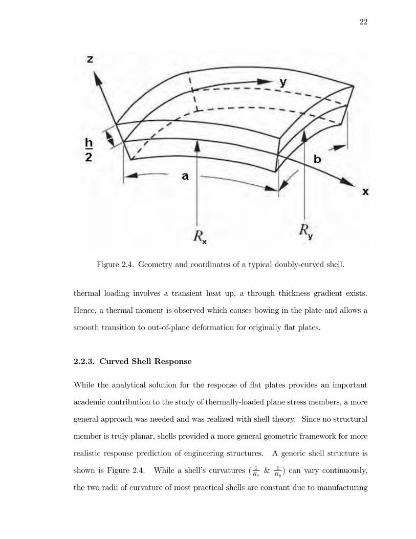
Figure 2.4. Geometry and coordinates of a typical doubly-curved shell.
thermal loading involves a transient heat up, a through thickness gradient exists.
Hence, a thermal moment is observed which causes bowing in the plate and allows a
smooth transition to out-of-plane deformation for originally �at plates.
2.2.3. Curved Shell Response
While the analytical solution for the response of �at plates provides an important
academic contribution to the study of thermally-loaded plane stress members, a more
general approach was needed and was realized with shell theory. Since no structural
member is truly planar, shells provided a more general geometric framework for more
realistic response prediction of engineering structures. A generic shell structure is
shown is Figure 2.4. While a shell�s curvatures ( 1Rx& 1
Ry) can vary continuously,
the two radii of curvature of most practical shells are constant due to manufacturing
23
constraints. As both radii approach in�nity, the �at plate solution is recovered.
Moreover, as a single radius is increased, the geometry approaches that of a cylinder.
The nonlinear equations for the response of the shell are more complicated than that
of the �at plate due to the presence of the initial curvature. The compatibility and
transverse equilibrium equations for a thermally loaded shell are given by Eqs. 2.14
and 2.15, respectively.
1
Ehr4� =
�@2w
@x@y
�2� @
2w
@x2� @
2w
@y2�(2.14)
1
Rx
@2w
@y2� 1
Ry
@2w
@x2� 1
Ehr2NT
Dr4w =@2w
@x2� @
2�
@y2+@2w
@y2� @
2�
@x2� 2 @
2�
@x@y� @
2w
@x@y+(2.15)
1
Rx
@2�
@y2+1
Ry
@2�
@x2� 1
(1� �)r2MT
The Airy stress function, �, as well as NT and MT are identical to that employed in
the �at plate equations. Many texts and articles exist which address the formulation
and solution of shell equations for mechanical, transverse loading. Some of the
earliest works can be found in [18],[19],[20],[21],and [22]. However, with respect to
thermal loading, the number of publications is more limited. The text by Langhaar
[23] is one of the few which includes the thermal load terms in the development
of the equations for shell theory. Most references to thermally loaded structures
which include instabilities are found in articles. Some of the �rst publications which
addressed thermoelastic response and stability of shells are found in the works by
Ho¤ [24], [25], and [26]. In these articles, geometric symmetry is used to reduce
the computational burden as the solution domains are chosen to be cylindrical and
conical.
24
2.2.3.1. In-plane Temperature Gradient. More applicable to the current work
with respect to geometry is the article by Mahayni [27]. Mahayni investigated the
thermal stability of isotropic nonlinear shallow shells subjected to an in-plane tem-
perature gradient. A sinusoidal solution is assumed for the transverse displacement,
w, which satis�es the zero displacement condition. A stress function is proposed
which satis�es Eq. 2.14 exactly. The transverse equilibrium Eq. 2.15 is then solved
by employing a Galerkin method to approximate the solution. Rx in Figure 2.4 is
chosen to be 1, so that the shell panel is singly-curved. Mahayni�s geometry di¤ers
slightly from that in Figure 2.4 in that the origin of the coordinate axes are located at
the center of the �gure with domain described by �a=2 � x � a=2, �b=2 � y � b=2,
and �h=2 � z � h=2. The positive direction of z is also reversed such that it points
toward the center of curvature. With u, v, and w as the displacement components
of a point on the middle surface, the internal forces can be represented by integrating
the stresses through the thickness,
Nx =
Z h=2
�h=2�xdz = [
Eh
1� �2@u
@x� kxw +
1
2(@w
@x)2(2.16)
+�
�@v
@y� kyw +
1
2(@w
@y)2�]� NT
1� �
Ny =
Z h=2
�h=2�ydz = [
Eh
1� �2@v
@y� kyw +
1
2(@w
@y)2(2.17)
+�
�@u
@x� kxw +
1
2(@w
@x)2�]� NT
1� �
Nxy =
Z h=2
�h=2�xydz =
Eh
2(1 + �)
�@u
@y+@v
@x+@w
@x
@w
@y
�(2.18)
25
and
Mx = �D(@2w
@x2+ �
@2w
@y2)� MT
(1� �)(2.19)
My = �D(@2w
@y2+ �
@2w
@x2)� MT
(1� �)(2.20)
Mxy = (1� �)D @2w
@x@y(2.21)
The temperature distribution is assumed constant through the thickness and circum-
ferential directions but varies parabolically from x = 0 to a such that
(2.22) T = [f + k(x� a)2]
where
k =e� fa2
=�T
a2
�T = Temperature di¤erence
f = Tx=a
e = Tx=0
A solution for the transverse displacement which satis�es the prescribed boundary
condition is given by
(2.23) w =
1Xn=1;2;3;:::
An(cos�x
acos
�y
b)n =
1XAn
n=1;2;3;:::
n
26
where An are undetermined coe¢ cients. The solution of equation 2.14 with Rx !1
and Ry = R, is given by
� = Eh
��2
ab
�2��A12
�(cos 2�x
a�2�a
�4 + cos 2�yb�2�b
�4)
(2.24)
+Eh
R
��a
�2A1
8><>: cos �xacos �y
bh��a
�2+��b
�2i29>=>;� � y
2
2� � x
2
2� Ehck
12x4
The solution presented in Mahayni contains a 24 in the denominator of the last term
instead of the 12 used in this work. In fact, the stress function in [27] does not
satisfy equation 2.14. Therefore the equations derived from this point forward in
this development will di¤er from that found in [27]. Also, note that � is used in this
section to denote a reaction force as opposed its typical use as coe¢ cient of thermal
expansion. The variables used in this section were employed to permit the interested
reader to most easily compare results with the original work
The Galerkin method is used to determine the unknown coe¢ cient, A1. A residual
equation is formed from the transverse equilibrium equation, 2.15, by rearranging such
that the right hand side of the equation is zero. Denoting this residual by Q, the
error is minimized by determining A1 such that
(2.25)Z a=2
�a=2
Z b=2
�b=2Q n dx dy = 0
The following dimensionless quantities are de�ned to facilitate the solution,
Ky =b2
R h; � =
a
b; Z1 =
A1h
(2.26)
K =a2b2
h2ck; Px =
�b2
Eh3; and Py =
�a2
Eh3
where c is the coe¢ cient of thermal expansion
27
Upon completing the integration in Eq. 2.25, and incorporating the non-dimensional
quantities Eq. 2.26, a cubic equation in Z1 is obtained.
�3�8(1 + �2)2(1 + �4)
�Z31 �
�32 Ky�
4�4(17 + 2�2 + �4)�Z21 + [�
4�8(1 + �2)4
(�2 � 1)
(2.27)
+48 K2y�
4�4 + 24 K �4�4 � 4�6(12 Px + 12 Py +K �2)(�+ �3)2] Z1
�1536 K Ky�4(1 + �2)2 + 192 Ky�
2(4 Py +K �2)(�+ �3)2 = 0
It should be noted here that the non-dimensional quantities for Px and Py again di¤er
from that published in [27]. In this work, both Px and Py contain an additional power
of h in their de�nition making the quantities dimensionless. Without this de�nition
of dimensionless force, Eq. 2.27 would contain both dimensionless and dimensional
quantities (e.g., h). These discrepancies do alter the results presented in [27] and
are therefore presented in this work for completeness.
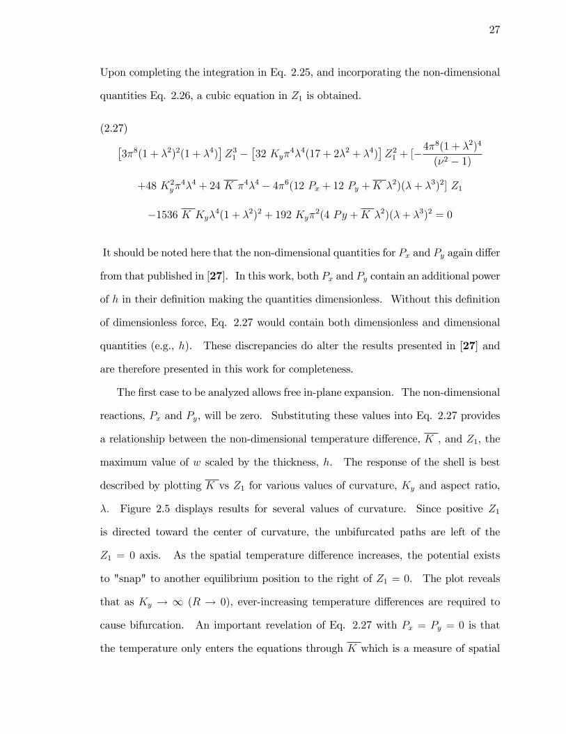
The �rst case to be analyzed allows free in-plane expansion. The non-dimensional
reactions, Px and Py, will be zero. Substituting these values into Eq. 2.27 provides
a relationship between the non-dimensional temperature di¤erence, K , and Z1, the
maximum value of w scaled by the thickness, h. The response of the shell is best
described by plotting K vs Z1 for various values of curvature, Ky and aspect ratio,
�: Figure 2.5 displays results for several values of curvature. Since positive Z1
is directed toward the center of curvature, the unbifurcated paths are left of the
Z1 = 0 axis. As the spatial temperature di¤erence increases, the potential exists
to "snap" to another equilibrium position to the right of Z1 = 0. The plot reveals
that as Ky ! 1 (R ! 0), ever-increasing temperature di¤erences are required to
cause bifurcation. An important revelation of Eq. 2.27 with Px = Py = 0 is that
the temperature only enters the equations through K which is a measure of spatial
28
Figure 2.5. Load de�ection curve for � = :30, � = 1, and Px = Py = 0.
temperature di¤erence. Therefore, if a constant temperature of any magnitude is
prescribed, buckling is not predicted for this set of boundary conditions for �nite
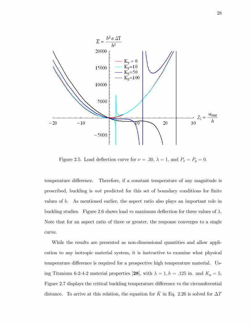
values of b. As mentioned earlier, the aspect ratio also plays an important role in
buckling studies. Figure 2.6 shows load vs maximum de�ection for three values of �.
Note that for an aspect ratio of three or greater, the response converges to a single
curve.
While the results are presented as non-dimensional quantities and allow appli-
cation to any isotropic material system, it is instructive to examine what physical
temperature di¤erence is required for a prospective high temperature material. Us-
ing Titanium 6-2-4-2 material properties [28], with � = 1; h = :125 in. and Ky = 5,
Figure 2.7 displays the critical buckling temperature di¤erence vs the circumferential
distance. To arrive at this relation, the equation for �K in Eq. 2.26 is solved for �T
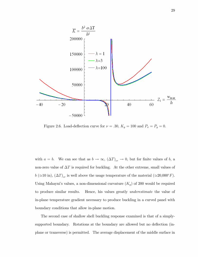
29
Figure 2.6. Load-de�ection curve for � = :30, Ky = 100 and Px = Py = 0.
with a = b. We can see that as b ! 1, (�T )cr ! 0, but for �nite values of b, a
non-zero value of �T is required for buckling. At the other extreme, small values of
b ('10 in), (�T )cr is well above the usage temperature of the material ('20,000�F ).
Using Mahayni�s values, a non-dimensional curvature (Ky) of 200 would be required
to produce similar results. Hence, his values greatly underestimate the value of
in-plane temperature gradient necessary to produce buckling in a curved panel with
boundary conditions that allow in-plane motion.
The second case of shallow shell buckling response examined is that of a simply-
supported boundary. Rotations at the boundary are allowed but no de�ection (in-
plane or transverse) is permitted. The average displacement of the middle surface in
30
Figure 2.7. Critical spatial temperature di¤erence �T vs circumferen-tial distance b for titanium alloy with Ky=5 and � = 1
the x-direction is given by the integral
(2.28) ex = �1
a
Z a=2
�a=2
@u
@xdx
However, this average varies in the y-direction. Hence, the integral average over the
y-coordinate is
(2.29) �ex =1
b
Z b=2
�b=2exdy
The constitutive equation provides a relation between @u@xand the dependent variables
(equation 2.30).
(2.30)@u
@x=
1
Eh(@2�
@y2� � @
2�
@x2)� 1
2(@w
@x)2 + cT
31
Carrying out the integrations in Eqs. 2.28 and 2.29, and equating �ex = 0, an equation
containing Px and Py is generated. This process is similarly carried out for �ey = 0
resulting in a second equation containing Px and Py. This system is solved for Px
and Py and substituted into Eq. 2.27. The governing equation for the panel with
restrained edges is given by
3�8(1 + �2)2(�3� 4�2� + �2 + �4(�3 + �2))Z31+(2.31)
32 Ky�4�2(3� + �2(8 + 6� � 5�2) + �4(8 + 3� � 2�2)� �6(�4 + �2))Z21+
(�4�8(1 + �2)4 + 48 �f �6(1 + �2)3(1 + �) + 52 �K�6�2(1 + �2)3(1 + �)�
3072 K2y�
4(�2 � 1) + 48 K2y�
4�4(�2 � 1) + 24 �K�4�2(�+ �3)2(�2 � 1))Z1�
768 �f Ky�2�2(1 + �2)2(1 + �)� 1536 �K Ky�
4(1 + �2)2(�2 � 1)+
64 �K Ky�2�4(1 + �2)2(�15� 13� + 2�2) = 0
where
�f =cfa2
h2
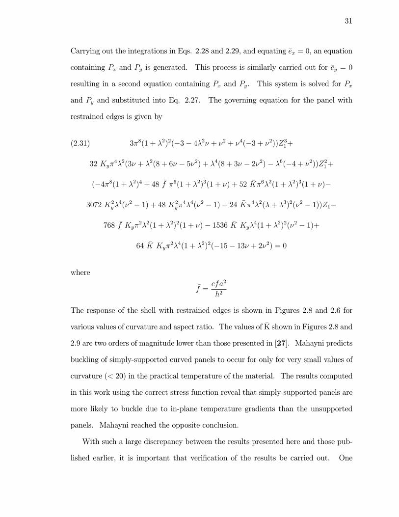
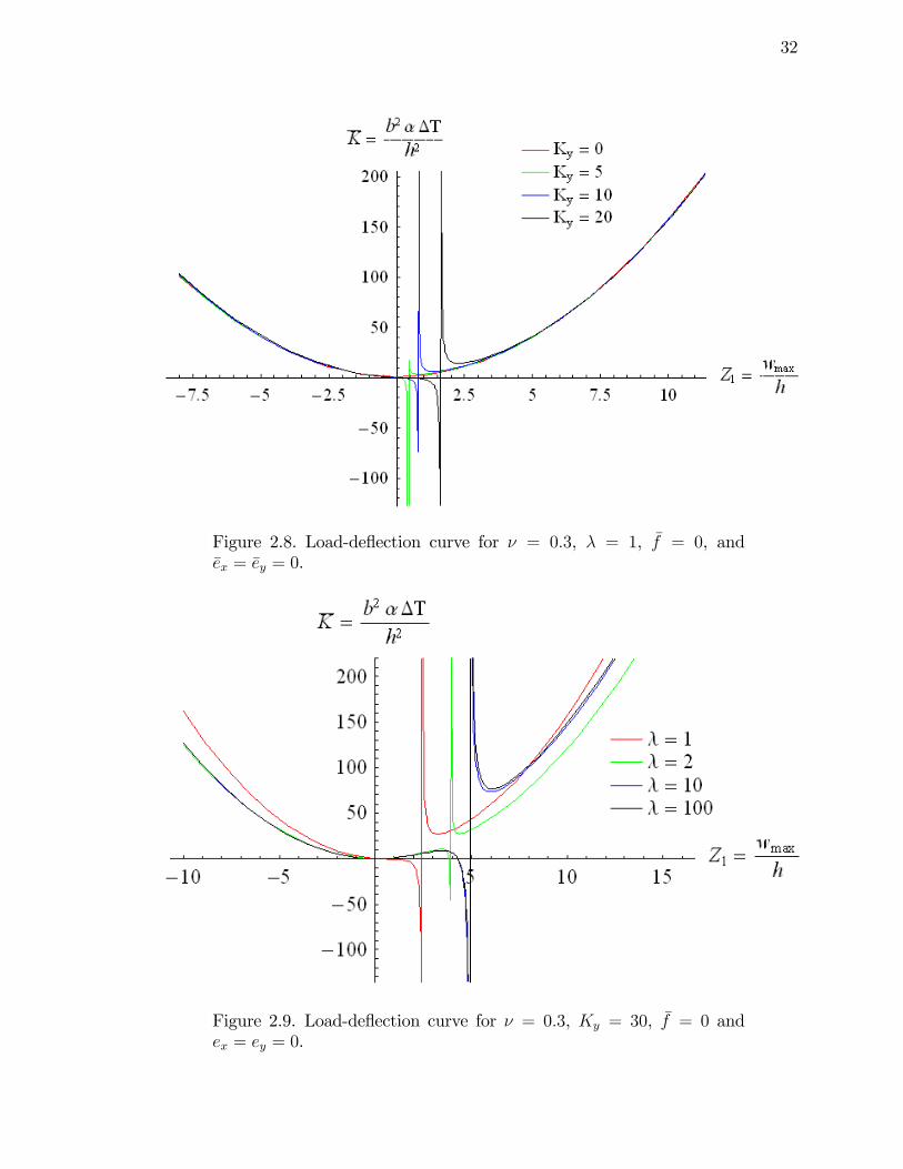
The response of the shell with restrained edges is shown in Figures 2.8 and 2.6 for
various values of curvature and aspect ratio. The values of K̄ shown in Figures 2.8 and
2.9 are two orders of magnitude lower than those presented in [27]. Mahayni predicts
buckling of simply-supported curved panels to occur for only for very small values of
curvature (< 20) in the practical temperature of the material. The results computed
in this work using the correct stress function reveal that simply-supported panels are
more likely to buckle due to in-plane temperature gradients than the unsupported
panels. Mahayni reached the opposite conclusion.
With such a large discrepancy between the results presented here and those pub-
lished earlier, it is important that veri�cation of the results be carried out. One
32
Figure 2.8. Load-de�ection curve for � = 0:3, � = 1, �f = 0, and�ex = �ey = 0.
Figure 2.9. Load-de�ection curve for � = 0:3, Ky = 30, �f = 0 andex = ey = 0.
33
Figure 2.10. Load-de�ection curve for � = 1, � = 0:3, Ky = 0, K = 0,and �ex = �ey = 0.
important di¤erence between the unrestrained and simply-supported conditions is the
presence of �f . Since �f contains an explicit reference to the temperature, buckling can
occur devoid of an in-plane temperature gradient. Since other, independent analyt-
ical solutions exist for constant temperature buckling solutions of simply-supported
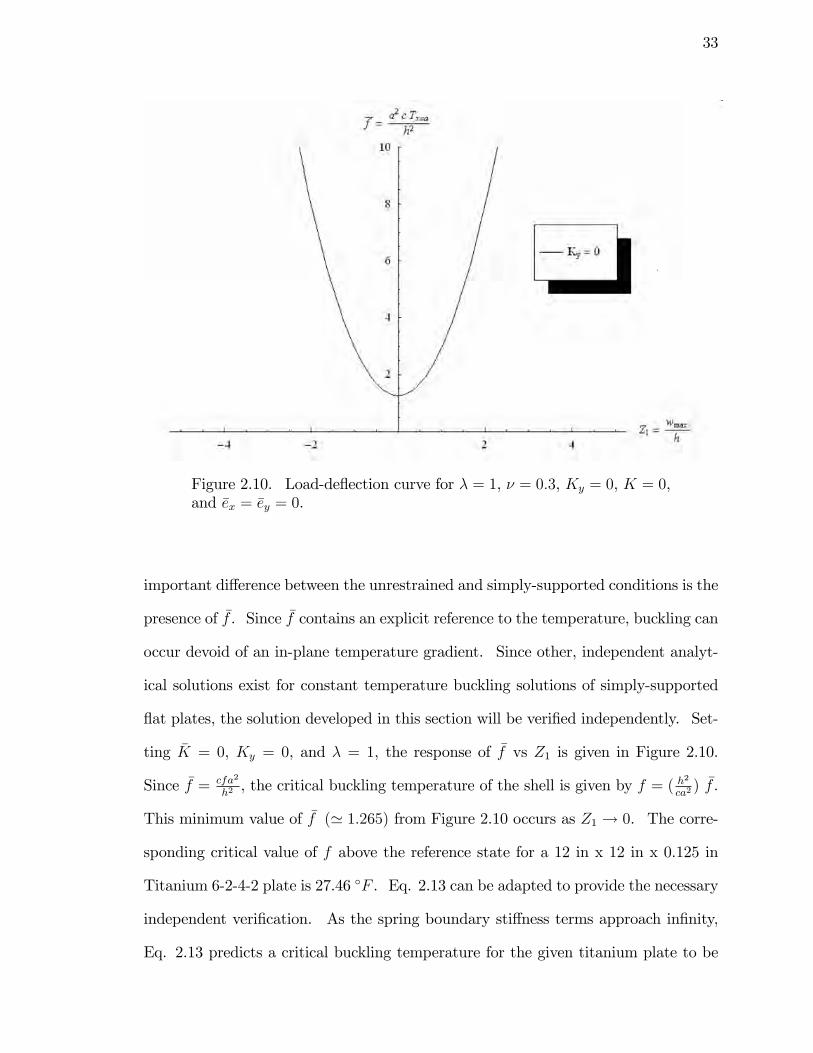
�at plates, the solution developed in this section will be veri�ed independently. Set-
ting �K = 0, Ky = 0, and � = 1, the response of �f vs Z1 is given in Figure 2.10.
Since �f = cfa2
h2, the critical buckling temperature of the shell is given by f = ( h
2
ca2) �f .
This minimum value of �f (' 1:265) from Figure 2.10 occurs as Z1 ! 0. The corre-
sponding critical value of f above the reference state for a 12 in x 12 in x 0.125 in
Titanium 6-2-4-2 plate is 27.46 �F . Eq. 2.13 can be adapted to provide the necessary
independent veri�cation. As the spring boundary sti¤ness terms approach in�nity,
Eq. 2.13 predicts a critical buckling temperature for the given titanium plate to be
34
T =27.46 �F . Therefore, the equations derived in this section reduce to the classical
�at plate buckling solution and provide a measure of veri�cation.
The major conclusions that can be deduced from this study are (i) as initial cur-
vature increases, larger spatial gradients and/or higher temperatures are required to
initiate buckling for both cases; (ii) much larger temperature di¤erences are required
to initiate buckling in the unrestrained case than in the simply-supported scenario,
and (iii) the aspect ratio in�uences the response to a much greater degree in the
simply-supported case.
While the previous study provides insight into the onset of buckling and post-
buckling response of a curved panel, stresses obtained from such a model are highly
inaccurate. The one-term approximation of the transverse displacement is not su¢ -
cient to resolve stresses accurately. Even though de�ections may be fairly accurate,
the second derivatives of the approximate de�ections may deviate widely from their
proper values. Consequently, when de�ections are used to calculate stresses, a high
degree of accuracy may be required [23]. This is not unlike the displacement �nite
element formulation where higher mesh density and/or higher order polynomials are
needed for stress convergence [29]. Since two and three-dimensional nonlinear prob-
lems typically require approximate methods like the Galerkin method used above, in
the next section a one-dimensional nonlinear model is solved to gain insight into the
stress behavior of thermally-loaded shell structures and the boundary loads generated
from employing common sti¤ening methods.
2.3. Straight Beam Model
2.3.1. Fixed End Conditions
A unit width strip model (Figure 2.11), will be used to demonstrate the non-intuitive
nature of sti¤ening in an elevated temperature thermoelastic environment. The strip
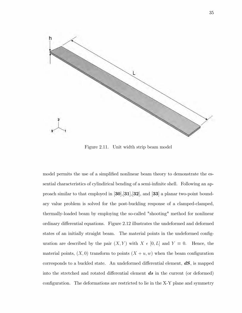
35
Figure 2.11. Unit width strip beam model
model permits the use of a simpli�ed nonlinear beam theory to demonstrate the es-
sential characteristics of cylindirical bending of a semi-in�nite shell. Following an ap-
proach similar to that employed in [30],[31],[32], and [33] a planar two-point bound-
ary value problem is solved for the post-buckling response of a clamped-clamped,
thermally-loaded beam by employing the so-called "shooting" method for nonlinear
ordinary di¤erential equations. Figure 2.12 illustrates the undeformed and deformed
states of an initially straight beam. The material points in the undeformed con�g-
uration are described by the pair (X;Y ) with X � [0; L] and Y � 0. Hence, the
material points, (X; 0) transform to points (X + u;w) when the beam con�guration
corresponds to a buckled state. An undeformed di¤erential element, dS, is mapped
into the stretched and rotated di¤erential element ds in the current (or deformed)
con�guration. The deformations are restricted to lie in the X-Y plane and symmetry
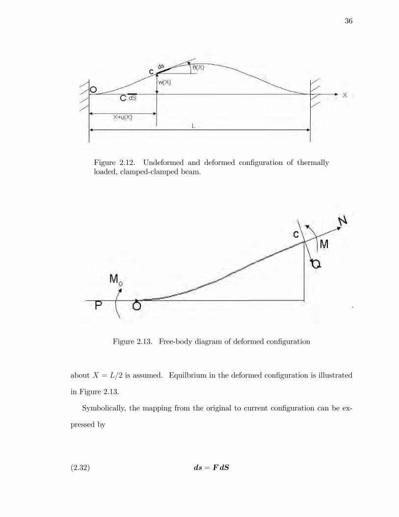
36
Figure 2.12. Undeformed and deformed con�guration of thermallyloaded, clamped-clamped beam.
Figure 2.13. Free-body diagram of deformed con�guration
about X = L=2 is assumed. Equilbrium in the deformed con�guration is illustrated
in Figure 2.13.
Symbolically, the mapping from the original to current con�guration can be ex-
pressed by
(2.32) ds = FdS
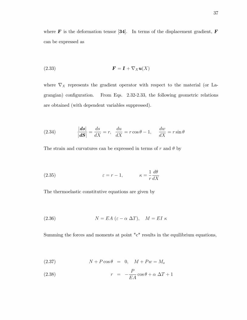
37
where F is the deformation tensor [34]. In terms of the displacement gradient, F
can be expressed as
(2.33) F = I +rXu(X)
where rX represents the gradient operator with respect to the material (or La-
grangian) con�guration. From Eqs. 2.32-2.33, the following geometric relations
are obtained (with dependent variables suppressed).
(2.34)jdsjjdSj =
ds
dX= r;
du
dX= r cos � � 1; dw
dX= r sin �
The strain and curvatures can be expressed in terms of r and � by
(2.35) " = r � 1; � =1
r
d�
dX
The thermoelastic constitutive equations are given by
(2.36) N = EA ("� � �T ); M = EI �
Summing the forces and moments at point "c" results in the equilibrium equations,
N + P cos � = 0; M + Pw =Mo(2.37)
r = � P
EAcos � + � �T + 1(2.38)
38
where s(X) is the arc length of the de�ected curve, r(X) is the stretch ratio of the
axial line, and �(X) is the cross-section rotation; N(X) is the axial internal force,
and M(X) is the internal bending moment; P is the constraint reaction force at
the clamped boundary; MO is the reaction moment at the constrained ends; E is
the Young�s modulus; � is the linear thermal expansion coe¢ cient; A is the cross-
sectional area; I is the second moment of area of the cross-section and �T is the
change in temperature of the uniform �eld. For this study, the material properties
will be assumed independent of the temperature.
For solution convenience, the following dimensionless variables will be used,
(�; bs; bu; bw;bh) =1
L(X; s; u; w; h); � = 2� �T;(2.39)
= L
rA
I; p =
PL2
EI; m =
MOL
EI(2.40)
the nonlinear system of dimensionless equations are given by
bs0(�) = r; bu0(�) = r cos � � 1;(2.41)
bw0(�) = r sin �; �
0(�) = r (m� p bw)(2.42)
p0(�) = m0(�) = 0(2.43)
where r = (�p cos �+ �)= 2+1 along with the following symmetric boundary condi-
tions,
39
bs(0) = bu(0) = bw(0) = �(0) = 0(2.44)
bu(12) = �(
1
2) = 0(2.45)
The dimensionless temperature � is treated as a prescribed parameter in the solu-
tion process. For values of � greater than 4�2, buckling occurs. To compute the large
displacement, out-of-plane deformation, a shooting method for solving nonlinear ordi-
nary di¤erential equations is utilized to solve the system of equations. Symbolically,
the system can be expressed as
dY (�)
d�= H(�;Y ; �) (0 < � <
1
2)(2.46)
B1Y (0) = f0 0 0 0gT ; B2Y (1
2) = f0 0gT
Y = fy1 y2 y3 y4 y5 y6 gT = fbs bu bw � m p gT
H = fr r cos y4 � 1 r sin y4 r(y5 � y3y6) 0 0gT
B1 =
2666666664
1 0 0 0 0 0
0 1 0 0 0 0
0 0 1 0 0 0
0 0 0 1 0 0
3777777775;B2 =
2640 1 0 0 0 0
0 0 0 1 0 0
375
In actuality, m and p are problem parameters. These load parameters are treated
as unknown functions of � forming a standard problem statement for accomodating
nonlinear boundary value problems with multiple parameters [35].
40
The shooting method for the solution of nonlinear ordinary di¤erential equations
involves reformulating the problem in terms of an initial value problem.
d eY (�)d�
= H(�; eY ; �) (0 < � <1
2)(2.47)
eY (0) = f0 0 0 0 m(0) p(0)gT
The initial value problem is iteratively solved using an appropriate integrator (i.e.,
4th-order Runka-Kutta) until the conditions at � = 1=2; match the prescribed values.
This problem can be treated as an optimization problem with the objective being
satisfaction of the end conditions while the unprescribed values at � = 0, m(0) =
p(0); are treated as design variables. If we de�ne the design variable vector dT =
fy5(0) y6(0)g ; then the current estimate of the initial value problem can be treated
as a function of the design variables,
d eY (�;d)d�
= H(�; eY (�; d); �)(2.48)
eY (0) = f0 0 0 0 d1 d2gT
The primal problem can be di¤erentiated to compute analytical sensitivities of
the response with respect to the design variables. This direct di¤erentiation method
is given by the two following pseudo problems. d eY (�;d)d�
!;d1
= H ; eY (�; eY (�; d); �) eY ;d1(2.49)
eY ;d1(0) = f0 0 0 0 1 0gT d eY (�;d)d�
!;d2
= H ; eY (�; eY (�; d); �) eY ;d2(2.50)
eY ;d2(0) = f0 0 0 0 0 1gT
41
The residual system of equations to be solved is expressed by
(2.51) �(d�) =� eY (�;d�)�B2Y (�)
��= 1
2
= 0
where d� denotes the optimal value of d. Expanding Eq. 2.51 in a �rst-order Taylor
series expansion,
�(d�) = �(di) +
�@�(d)
@d
�d=di
�di � 0(2.52)
�di � ��@�(d)
@d
��1d=di
�(di)(2.53)
di+1 = di +�di(2.54)
facilitates application of Newton�s method for the solution of the nonlinear system
with di the current estimate of the design variables.
Thermally buckled con�gurations are shown in Figure 2.14 for various values of � .
For a clamped-clamped isotropic beam, the maximum tensile stress will occur at the
clamped edge at the outermost �bers opposite the displacement. Hence for the case
under consideration, the maximum stress occurs at point "O" (Figure 2.13) on the
bottom side of the beam. One of the most common approaches to alleviating thermal
buckling is to increase the thickness of the panel. The minimal value of � for which
buckling occurs is computed by solution of the linearized eigenvalue problem in Eq.
2.46. The critical value of � at which buckling occurs is 4�2. From Eq. 2.39, with
� = 4�2 = 2� (�T )cr a decrease in increases the temperature change required for
buckling to occur. The non-dimensional thickness is related to 2 by
(2.55) 2 = L2A
I= L2
�h112h3
�=
12�h2
L2
� = 12bh2
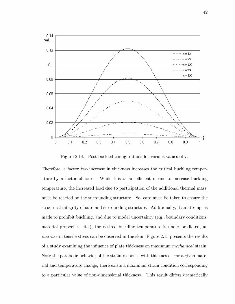
42
Figure 2.14. Post-buckled con�gurations for various values of � :
Therefore, a factor two increase in thickness increases the critical buckling temper-
ature by a factor of four. While this is an e¢ cient means to increase buckling
temperature, the increased load due to participation of the additional thermal mass,
must be reacted by the surrounding structure. So, care must be taken to ensure the
structural integrity of sub- and surrounding structure. Additionally, if an attempt is
made to prohibit buckling, and due to model uncertainty (e.g., boundary conditions,
material properties, etc.), the desired buckling temperature is under predicted, an
increase in tensile stress can be observed in the skin. Figure 2.15 presents the results
of a study examining the in�uence of plate thickness on maximum mechanical strain.
Note the parabolic behavior of the strain response with thickness. For a given mate-
rial and temperature change, there exists a maximum strain condition corresponding
to a particular value of non-dimensional thickness. This result di¤ers dramatically
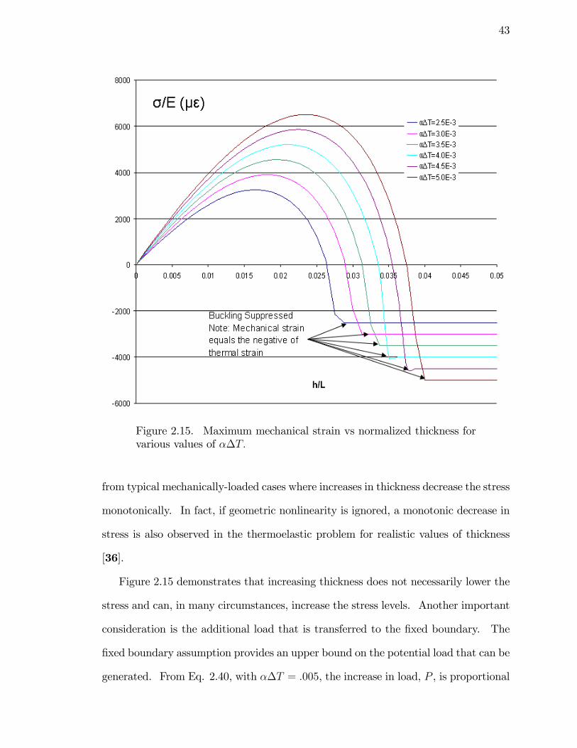
43
Figure 2.15. Maximum mechanical strain vs normalized thickness forvarious values of ��T:
from typical mechanically-loaded cases where increases in thickness decrease the stress
monotonically. In fact, if geometric nonlinearity is ignored, a monotonic decrease in
stress is also observed in the thermoelastic problem for realistic values of thickness
[36].
Figure 2.15 demonstrates that increasing thickness does not necessarily lower the
stress and can, in many circumstances, increase the stress levels. Another important
consideration is the additional load that is transferred to the �xed boundary. The
�xed boundary assumption provides an upper bound on the potential load that can be
generated. From Eq. 2.40, with ��T = :005, the increase in load, P , is proportional
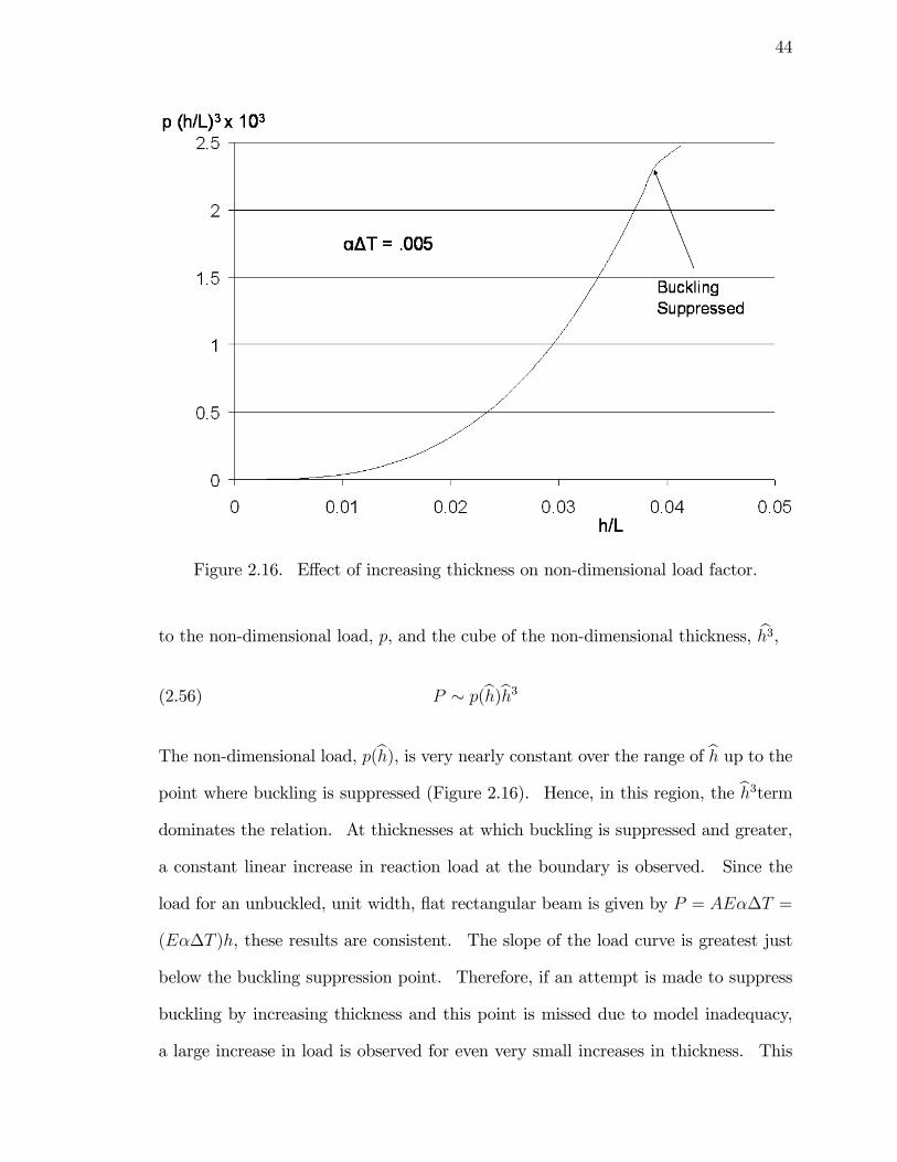
44
Figure 2.16. E¤ect of increasing thickness on non-dimensional load factor.
to the non-dimensional load, p, and the cube of the non-dimensional thickness, bh3,(2.56) P � p(bh)bh3The non-dimensional load, p(bh), is very nearly constant over the range of bh up to thepoint where buckling is suppressed (Figure 2.16). Hence, in this region, the bh3termdominates the relation. At thicknesses at which buckling is suppressed and greater,
a constant linear increase in reaction load at the boundary is observed. Since the
load for an unbuckled, unit width, �at rectangular beam is given by P = AE��T =
(E��T )h, these results are consistent. The slope of the load curve is greatest just
below the buckling suppression point. Therefore, if an attempt is made to suppress
buckling by increasing thickness and this point is missed due to model inadequacy,
a large increase in load is observed for even very small increases in thickness. This
45
behavior is similar to what was observed in the strain verses thickness behavior. The
primary conclusion to be drawn is that an increase in thickness results in a monotonic
increase in load to the boundary which, in a realistic structure, will be reacted by
sub- and surrounding structure. So material, being used to sti¤en a structure in a
thermal environment, should be used sparingly and judicously to accomplish the two
objectives of minimal boundary load increase and stress reduction.
2.3.2. Elastic End Conditions
In the previous section, �xed end conditions were exclusively considered. In this
section the in�uence of �exibility at the boundary will be addressed. With �exible
end conditions, the possibility exists that the results of the previous section could
be called into question. However, one indication that the conclusions reached in
the �xed end condition case will remain valid is given by the curve in Figure 2.3.
Note that at large values of relative spring sti¤ness, the curve is rather �at. This
implies that decreases in relative spring sti¤ness between the panel and the boundary
have little e¤ect on the buckling temperature when the boundary sti¤nesses are large.
Therefore, as the sti¤ness of the panel is increased (e.g., increasing thickness) relative
to the boundary sti¤ness, the initial indication is that stresses may not be reduced
until a given ratio of sti¤ness is obtained. This phenomenon is investigated in this
section.
Since the damage location of interest is coincident with the boundary, edge rota-
tions will again be suppressed, however, �nite edge displacements will be permitted as
thermal expansion takes place. Figure 2.17 illustrates the geometry in which linear
springs are placed at X = 0 and X = L. This choice of placement maintains symme-
try in the problem formulation. In [33], Vaz and Solano introduce a spring at X = 0
but maintain a simple-supported boundary at X = L which destroys symmetry in
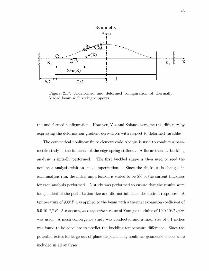
46
Figure 2.17. Undeformed and deformed con�guration of thermallyloaded beam with spring supports.
the undeformed con�guration. However, Vaz and Solano overcome this di¢ culty by
expressing the deformation gradient derivatives with respect to deformed variables.
The commerical nonlinear �nite element code Abaqus is used to conduct a para-
metric study of the in�uence of the edge spring sti¤ness. A linear thermal buckling
analysis is initially performed. The �rst buckled shape is then used to seed the
nonlinear analysis with an small imperfection. Since the thickness is changed in
each analysis run, the initial imperfection is scaled to be 5% of the current thickness
for each analysis performed. A study was performed to ensure that the results were
independent of the perturbation size and did not in�uence the desired responses. A
temperature of 900�F was applied to the beam with a thermal expansion coe¢ cient of
5.0�10�6=�F: A constant, at-temperature value of Young�s modulus of 10.0�106lbf=in2
was used. A mesh convergence study was conducted and a mesh size of 0.1 inches
was found to be adequate to predict the buckling temperature di¤erence. Since the
potential exists for large out-of-plane displacement, nonlinear geometric e¤ects were
included in all analyses.
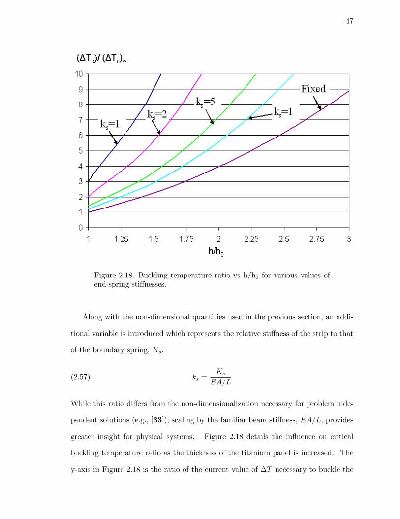
47
Figure 2.18. Buckling temperature ratio vs h/h0 for various values ofend spring sti¤nesses.
Along with the non-dimensional quantities used in the previous section, an addi-
tional variable is introduced which represents the relative sti¤ness of the strip to that
of the boundary spring, Ks.
(2.57) ks =Ks
EA=L
While this ratio di¤ers from the non-dimensionalization necessary for problem inde-
pendent solutions (e.g., [33]), scaling by the familiar beam sti¤ness, EA=L, provides
greater insight for physical systems. Figure 2.18 details the in�uence on critical
buckling temperature ratio as the thickness of the titanium panel is increased. The
y-axis in Figure 2.18 is the ratio of the current value of �T necessary to buckle the
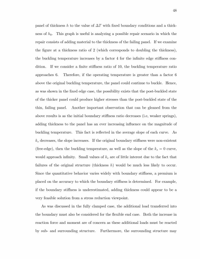
48
panel of thickness h to the value of �T with �xed boundary conditions and a thick-
ness of h0. This graph is useful is analyzing a possible repair scenario in which the
repair consists of adding material to the thickness of the failing panel. If we examine
the �gure at a thickness ratio of 2 (which corresponds to doubling the thickness),
the buckling temperature increases by a factor 4 for the in�nite edge sti¤ness con-
dition. If we consider a �nite sti¤ness ratio of 10, the buckling temperature ratio
approaches 6. Therefore, if the operating temperature is greater than a factor 6
above the original buckling temperature, the panel could continue to buckle. Hence,
as was shown in the �xed edge case, the possibility exists that the post-buckled state
of the thicker panel could produce higher stresses than the post-buckled state of the
thin, failing panel. Another important observation that can be gleaned from the
above results is as the initial boundary sti¤ness ratio decreases (i.e, weaker springs),
adding thickness to the panel has an ever increasing in�uence on the magnitude of
buckling temperature. This fact is re�ected in the average slope of each curve. As
ks decreases, the slope increases. If the original boundary sti¤ness were non-existent
(free-edge), then the buckling temperature, as well as the slope of the ks = 0 curve,
would approach in�nity. Small values of ks are of little interest due to the fact that
failures of the original structure (thickness h) would be much less likely to occur.
Since the quantitative behavior varies widely with boundary sti¤ness, a premium is
placed on the accuracy to which the boundary sti¤ness is determined. For example,
if the boundary sti¤ness is underestimated, adding thickness could appear to be a
very feasible solution from a stress reduction viewpoint.
As was discussed in the fully clamped case, the additional load transferred into
the boundary must also be considered for the �exible end case. Both the increase in
reaction force and moment are of concern as these additional loads must be reacted
by sub- and surrounding structure. Furthermore, the surrounding structure may
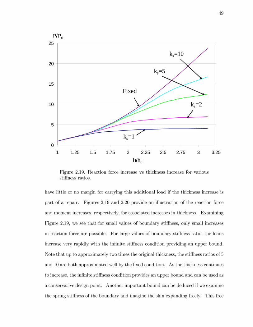
49
0
5
10
15
20
25
1 1.25 1.5 1.75 2 2.25 2.5 2.75 3 3.25
Fixed
ks=10
ks=5
ks=2
ks=1
h/h0
P/P0
0
5
10
15
20
25
1 1.25 1.5 1.75 2 2.25 2.5 2.75 3 3.25
Fixed
ks=10
ks=5
ks=2
ks=1
h/h0
P/P0
Figure 2.19. Reaction force increase vs thickness increase for varioussti¤ness ratios.
have little or no margin for carrying this additional load if the thickness increase is
part of a repair. Figures 2.19 and 2.20 provide an illustration of the reaction force
and moment increases, respectively, for associated increases in thickness. Examining
Figure 2.19, we see that for small values of boundary sti¤ness, only small increases
in reaction force are possible. For large values of boundary sti¤ness ratio, the loads
increase very rapidly with the in�nite sti¤ness condition providing an upper bound.
Note that up to approximately two times the original thickness, the sti¤ness ratios of 5
and 10 are both approximated well by the �xed condition. As the thickness continues
to increase, the in�nite sti¤ness condition provides an upper bound and can be used as
a conservative design point. Another important bound can be deduced if we examine
the spring sti¤ness of the boundary and imagine the skin expanding freely. This free
50
0
2
4
6
8
10
12
1 1.25 1.5 1.75 2 2.25 2.5 2.75 3 3.25
Fixed
ks=2
ks=5
ks=10
ks=1
h/h0
M/M0
0
2
4
6
8
10
12
1 1.25 1.5 1.75 2 2.25 2.5 2.75 3 3.25
Fixed
ks=2
ks=5
ks=10
ks=1
h/h0
M/M0
Figure 2.20. Moment increase vs thickness increase for various sti¤ness ratios
in-plane expansion multiplied by the spring sti¤ness provides an upper bound on the
reaction force produced. While this load is not theoretically possible since the skin
is not free to expand unabated, it does provide a useful metric for comparison if the
boundary sti¤ness ratio is available to the analysis.
The moment curves in Figure 2.20 demonstrate similar behavior to that found
in the previous clamped beam study. The moment initially increases with increas-
ing thickness, reaches a maximum and then tails o¤ as out-of-plane deformation is
eventually suppressed due to the buckling temperature exceeding the operation tem-
perature. Again we notice that as the boundary sti¤ness is reduced, less potential
exists for generating large moments. And as in the reaction force, the in�nite sti¤ness
case provides an upper bound on possible moment increases. Also, the sti¤ness ratio
of 10 is su¢ ciently approximated by the �xed case up to thickness ratios of 2.
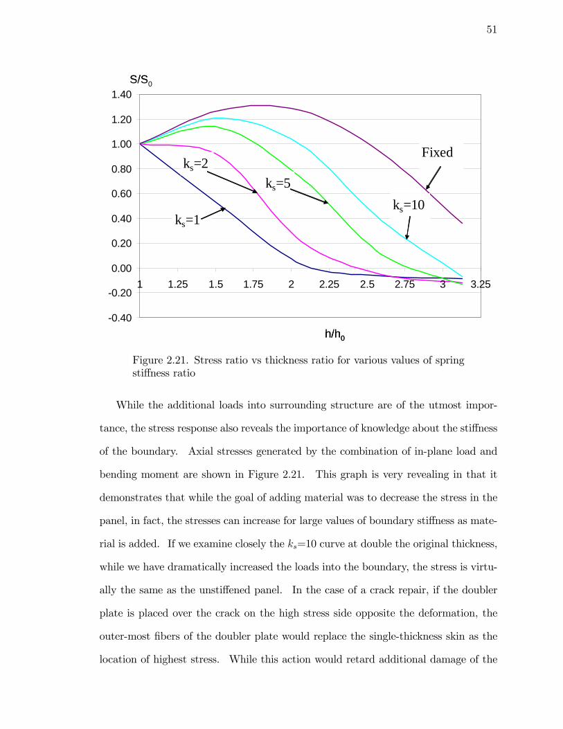
51
0.40
0.20
0.00
0.20
0.40
0.60
0.80
1.00
1.20
1.40
1 1.25 1.5 1.75 2 2.25 2.5 2.75 3 3.25
ks=2Fixed
ks=5ks=10
ks=1
S/S0
h/h0
0.40
0.20
0.00
0.20
0.40
0.60
0.80
1.00
1.20
1.40
1 1.25 1.5 1.75 2 2.25 2.5 2.75 3 3.25
ks=2Fixed
ks=5ks=10
ks=1
S/S0
h/h0
Figure 2.21. Stress ratio vs thickness ratio for various values of springsti¤ness ratio
While the additional loads into surrounding structure are of the utmost impor-
tance, the stress response also reveals the importance of knowledge about the sti¤ness
of the boundary. Axial stresses generated by the combination of in-plane load and
bending moment are shown in Figure 2.21. This graph is very revealing in that it
demonstrates that while the goal of adding material was to decrease the stress in the
panel, in fact, the stresses can increase for large values of boundary sti¤ness as mate-
rial is added. If we examine closely the ks=10 curve at double the original thickness,
while we have dramatically increased the loads into the boundary, the stress is virtu-
ally the same as the unsti¤ened panel. In the case of a crack repair, if the doubler
plate is placed over the crack on the high stress side opposite the deformation, the
outer-most �bers of the doubler plate would replace the single-thickness skin as the
location of highest stress. While this action would retard additional damage of the
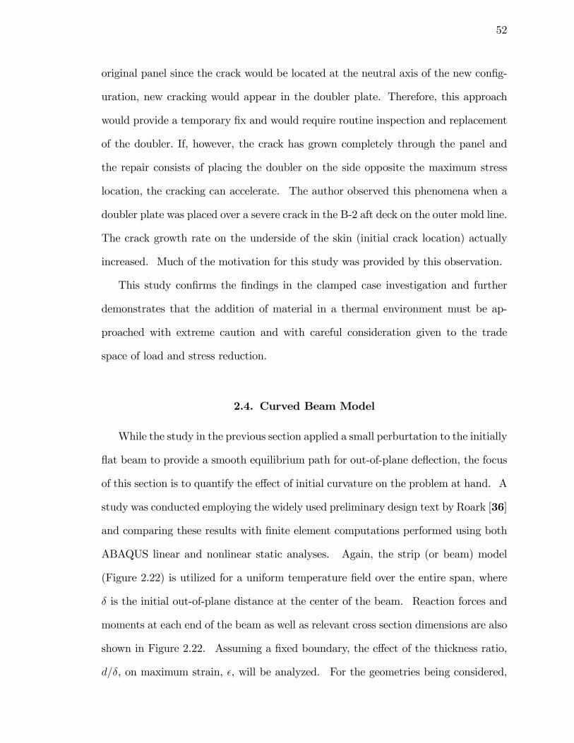
52
original panel since the crack would be located at the neutral axis of the new con�g-
uration, new cracking would appear in the doubler plate. Therefore, this approach
would provide a temporary �x and would require routine inspection and replacement
of the doubler. If, however, the crack has grown completely through the panel and
the repair consists of placing the doubler on the side opposite the maximum stress
location, the cracking can accelerate. The author observed this phenomena when a
doubler plate was placed over a severe crack in the B-2 aft deck on the outer mold line.
The crack growth rate on the underside of the skin (initial crack location) actually
increased. Much of the motivation for this study was provided by this observation.
This study con�rms the �ndings in the clamped case investigation and further
demonstrates that the addition of material in a thermal environment must be ap-
proached with extreme caution and with careful consideration given to the trade
space of load and stress reduction.
2.4. Curved Beam Model
While the study in the previous section applied a small perburtation to the initially
�at beam to provide a smooth equilibrium path for out-of-plane de�ection, the focus
of this section is to quantify the e¤ect of initial curvature on the problem at hand. A
study was conducted employing the widely used preliminary design text by Roark [36]
and comparing these results with �nite element computations performed using both
ABAQUS linear and nonlinear static analyses. Again, the strip (or beam) model
(Figure 2.22) is utilized for a uniform temperature �eld over the entire span, where
� is the initial out-of-plane distance at the center of the beam. Reaction forces and
moments at each end of the beam as well as relevant cross section dimensions are also
shown in Figure 2.22. Assuming a �xed boundary, the e¤ect of the thickness ratio,
d=�, on maximum strain, �, will be analyzed. For the geometries being considered,
53
Figure 2.22. Curved beam geometry and reaction forces.
the maximum strain will again occur at the clamped edges. With L = 12 inches (and
the values of � also in inches), Figures 2.23 - 2.26 detail the results of the investigation
for various values of an initial out-of-plane curvature of the panel which is described
by the �=L ratio. The linear �nite element solution and the Roark solution coincide
precisely. To achieve this agreement, a mesh density of 0.01 inches was required
(~1200 two-noded linear elements). For very small values of � (Figures 2.25 - 2.26)
there are large di¤erences between the linear solution (Roark�s or linear FEA) and the
nonlinear �nite element solution. The linear solutions make no distinction between
the deformed and undeformed con�guration. Therefore, as the two con�gurations
diverge, nonlinear geometric e¤ects must be included. The out-of-plane deformation
in these two cases is greater than the thickness and hence requires nonlinear analyses.
As the initial out-of-plane distance of the curved panel is increased (Figures 2.23
- 2.24), the out-of-plane deformation decreases which results in coalescence of the
linear and nonlinear solutions. Another important observation is that the maximum
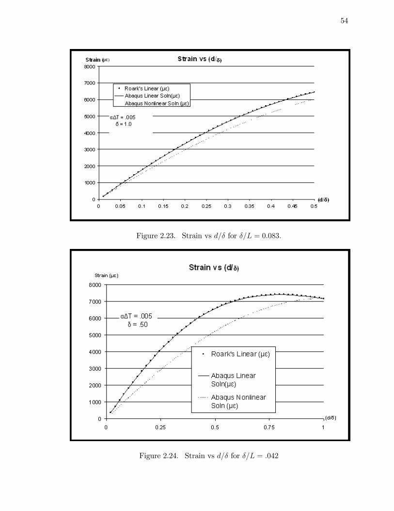
54
Figure 2.23. Strain vs d=� for �=L = 0:083:
Figure 2.24. Strain vs d=� for �=L = :042
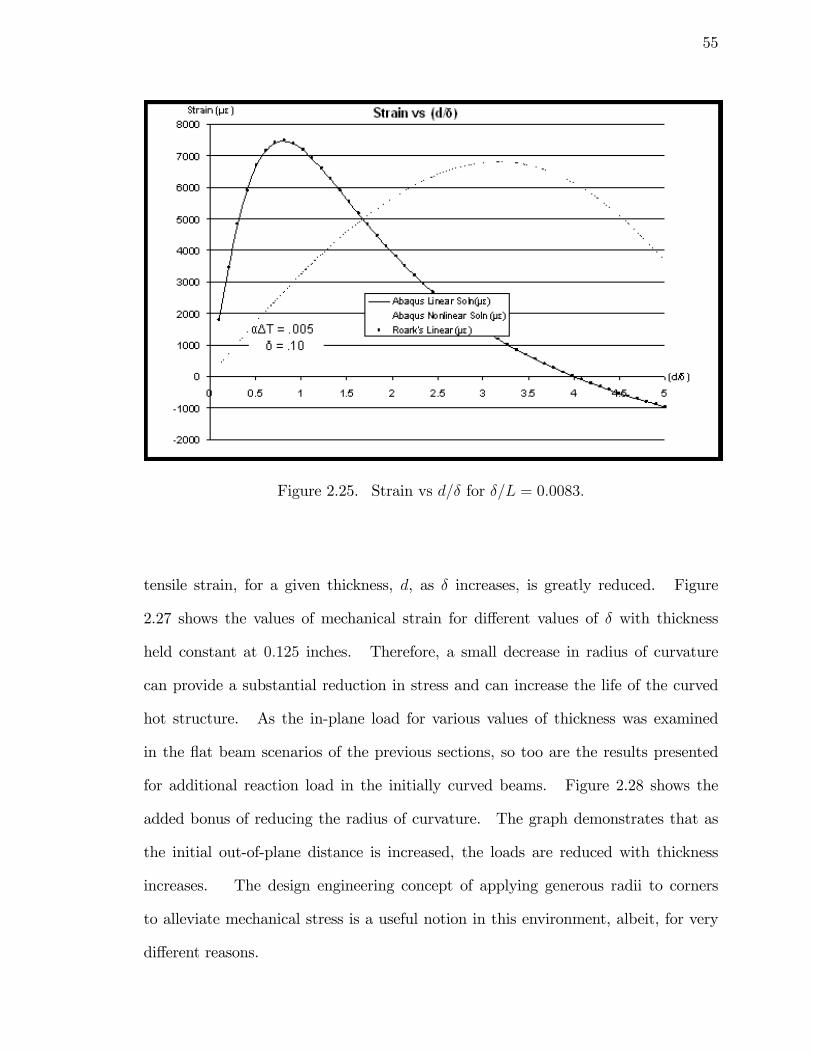
55
Figure 2.25. Strain vs d=� for �=L = 0:0083:
tensile strain, for a given thickness, d, as � increases, is greatly reduced. Figure
2.27 shows the values of mechanical strain for di¤erent values of � with thickness
held constant at 0:125 inches. Therefore, a small decrease in radius of curvature
can provide a substantial reduction in stress and can increase the life of the curved
hot structure. As the in-plane load for various values of thickness was examined
in the �at beam scenarios of the previous sections, so too are the results presented
for additional reaction load in the initially curved beams. Figure 2.28 shows the
added bonus of reducing the radius of curvature. The graph demonstrates that as
the initial out-of-plane distance is increased, the loads are reduced with thickness
increases. The design engineering concept of applying generous radii to corners
to alleviate mechanical stress is a useful notion in this environment, albeit, for very
di¤erent reasons.
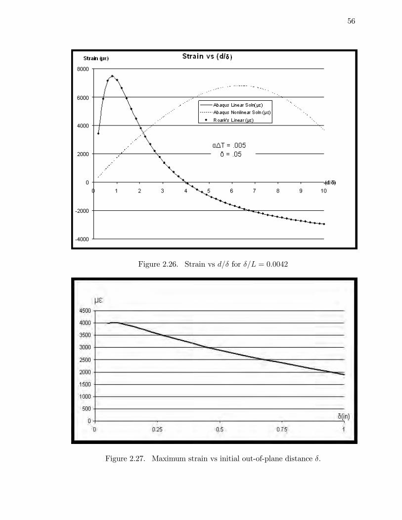
56
Figure 2.26. Strain vs d=� for �=L = 0:0042
Figure 2.27. Maximum strain vs initial out-of-plane distance �:
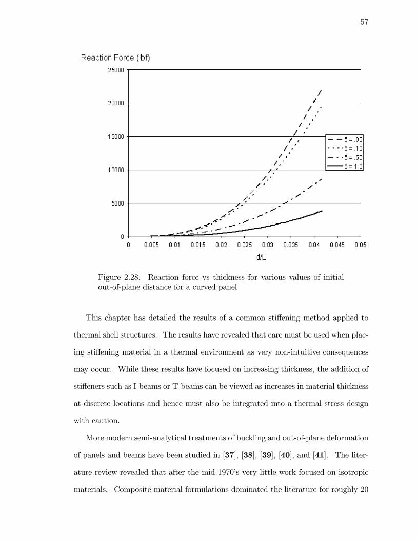
57
Figure 2.28. Reaction force vs thickness for various values of initialout-of-plane distance for a curved panel
This chapter has detailed the results of a common sti¤ening method applied to
thermal shell structures. The results have revealed that care must be used when plac-
ing sti¤ening material in a thermal environment as very non-intuitive consequences
may occur. While these results have focused on increasing thickness, the addition of
sti¤eners such as I-beams or T-beams can be viewed as increases in material thickness
at discrete locations and hence must also be integrated into a thermal stress design
with caution.
More modern semi-analytical treatments of buckling and out-of-plane deformation
of panels and beams have been studied in [37], [38], [39], [40], and [41]. The liter-
ature review revealed that after the mid 1970�s very little work focused on isotropic
materials. Composite material formulations dominated the literature for roughly 20
58
years while very recent work has focused on functionally-graded materials that al-
low very rapid (approaching continuous) material changes based on the local desired
properties. It is the author�s opinion that the particular revelations regarding the
thickness parameter that are the focus of much of this chapter were not produced
earlier due to two factors. Firstly, from a design standpoint, the solution to ther-
mally constrained structures is to permit expansion so the necessity of sti¤ening was
avoided. Secondly, when the focus of the research community turned toward com-
posite structures, the sti¤ness of the panel could now be in�uenced by a multitude
of material properties. To sti¤en a particular panel, attention was focused on the
reduced sti¤nesses of individual layers of the composite [42] as opposed to a simple
increase in cross section.
2.5. Chapter Summary
In this chapter we have detailed the inherent di¢ culties associated with thermo-
elastic design. Many of the traditional design concepts that designers are familiar
and comfortable with in a purely mechanically-loaded setting are highly non-optimal
when applied to structures whose response is due to thermal energy input. Sev-
eral examples of common aerospace structures were presented to demonstrate the
non-intuitive nature of sti¤ening strucures subjected to elevated temperature. The
entire concept of sti¤ening must be perceived di¤erently in this environment. Typ-
ically, when a designer intends to sti¤en a failing part, the intention is to reduce
the damage at that location by adding material. The conclusions in this chapter
reveal that sti¤ening thin shells in a thermal environment by adding material to the
damage location can actually increase the rate of damage. Therefore, to refer to this
process as sti¤ening is a misnomer. Because thermally-loaded structures in essence
provide their own loading through material expansion, the addition of material must
59
be approached cautiously. For additional material to provide a bene�cial outcome,
it must participate in the reaction of the original loading more than it contributes to
additional load in the vicinity of the critical design region. The other major concern
that was investigated in this chapter was the additional load that is reacted at the
idealized boundary conditions. While in this work, the boundaries are assumed both
clamped and simply-supported, in reality, sub- and surrounding structure provide the
constraint. When additional material is added to prevent damage or for restoration
of a damaged component, additional load is introduced and will be reacted by the
surrounding structure. This additional load must be managed and therefore provides
an upper bound on what is possible from a sti¤ening approach.
CHAPTER 3
Topology Optimization
3.1. Overview
Topology optimization of continuum structures has been an area of active research
for more than a decade. The topology optimization formulation seeks to determine
the optimal distribution of material and void within an initial design region. To
prevent the trivial solution for a sti¤ness objective (i.e., no void regions), a resource
constraint on the volume of material is generally enforced. Topology optimization
is distinguished from both sizing and shape optimization in that the �layout�of the
structure is unknown a priori. In fact, the structural layout is the computed quantity.
A sizing optimization problem commonly has as its design variables, parameters
such as thickness, area, or moment of area of a structural member. Sizing optimization
has the most straightforward implementation and has numerous analytical solutions
[43]. Sizing optimization has been incorporated in several structural mechanics codes
�two of which are ASTROS [44] and GENESIS [45].
Increasing in level of complexity, shape optimization involves the determination
of the boundary of a structure or structural member. Variational calculus provides a
framework for analytical solutions to shape optimization problems (e.g., the brachis-
tochrone function [46]). In a �nite element or boundary element formulation, the
boundary node locations are commonly taken as design variables [47]. Other vari-
ants parameterize the boundary by a conveniently chosen basis of B-splines [48] or
structural frequency mode shapes obtained from a former analysis. While shape opti-
mization provides the designer with greater �exibility than simple sizing, the locations
60
61
of material and void are necessarily speci�ed by the designer at the preliminary design
stage which limits the possible topologies generated.
A plethora of various methods have appeared in the literature which address the
topology optimization . Since the topology problem can be formulated as a combi-
natorial optimization problem with each material point potentially having a value of
0 (void) or 1 (material), genetic algorithms (GA�s) [49] and [50] and heuristic meth-
ods [51] have been used to determine global optima. Combinatorial (or zeroth order)
methods which do not require gradient information are somewhat limited with respect
to problem size and will not be pursued in this work. The most popular methods
are based on gradient search algorithms (also known as mathematical programming
methods). These gradient search methods can be further subdivided based on how
the discrete design variable is treated. The discrete problem can be transformed to a
continuous representation by either introducing a microscopically composite material
using the homogenization method [52] or employing an interpolation based on the
Simpli�ed Isotropic Material with Penalization (SIMP) method [53]. In contrast,
other methods such as the evolutionary structural optimization (ESO) method [54],
more directly address the discrete variable problem by removing elements from the
�nite element mesh. One relatively new approach which does not require a discrete
to continuous transformation is the Level Set Method [55]. This method embeds a
series of macroscopic holes in a topological domain. These embedded boundaries can
move and resize based on the solution to a �Hamilton-Jacobi-type�equation [56].
In the following sections, previous work in the area of topology optimization will
be detailed. The subsequent summaries are by no means exhaustive but provide a
general overview of the subject areas along with references for the interested reader
to gain further insight.
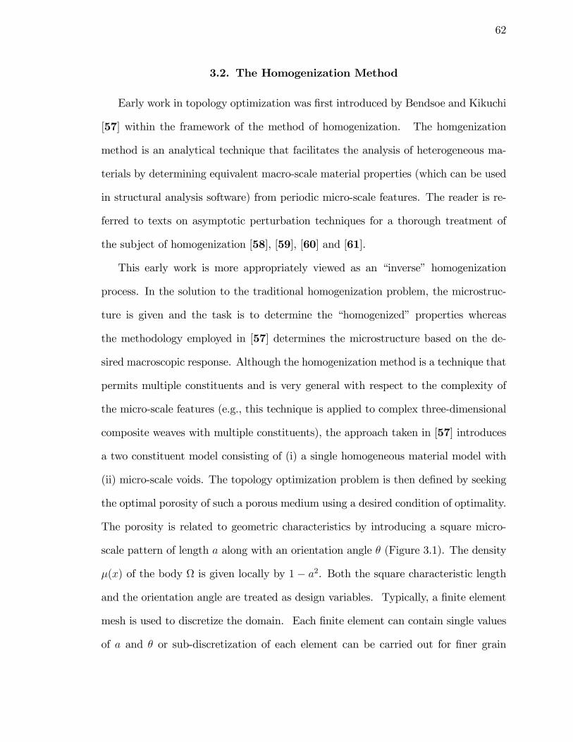
62
3.2. The Homogenization Method
Early work in topology optimization was �rst introduced by Bendsoe and Kikuchi
[57] within the framework of the method of homogenization. The homgenization
method is an analytical technique that facilitates the analysis of heterogeneous ma-
terials by determining equivalent macro-scale material properties (which can be used
in structural analysis software) from periodic micro-scale features. The reader is re-
ferred to texts on asymptotic perturbation techniques for a thorough treatment of
the subject of homogenization [58], [59], [60] and [61].
This early work is more appropriately viewed as an �inverse� homogenization
process. In the solution to the traditional homogenization problem, the microstruc-
ture is given and the task is to determine the �homogenized� properties whereas
the methodology employed in [57] determines the microstructure based on the de-
sired macroscopic response. Although the homogenization method is a technique that
permits multiple constituents and is very general with respect to the complexity of
the micro-scale features (e.g., this technique is applied to complex three-dimensional
composite weaves with multiple constituents), the approach taken in [57] introduces
a two constituent model consisting of (i) a single homogeneous material model with
(ii) micro-scale voids. The topology optimization problem is then de�ned by seeking
the optimal porosity of such a porous medium using a desired condition of optimality.
The porosity is related to geometric characteristics by introducing a square micro-
scale pattern of length a along with an orientation angle � (Figure 3.1). The density
�(x) of the body is given locally by 1 � a2. Both the square characteristic length
and the orientation angle are treated as design variables. Typically, a �nite element
mesh is used to discretize the domain. Each �nite element can contain single values
of a and � or sub-discretization of each element can be carried out for �ner grain
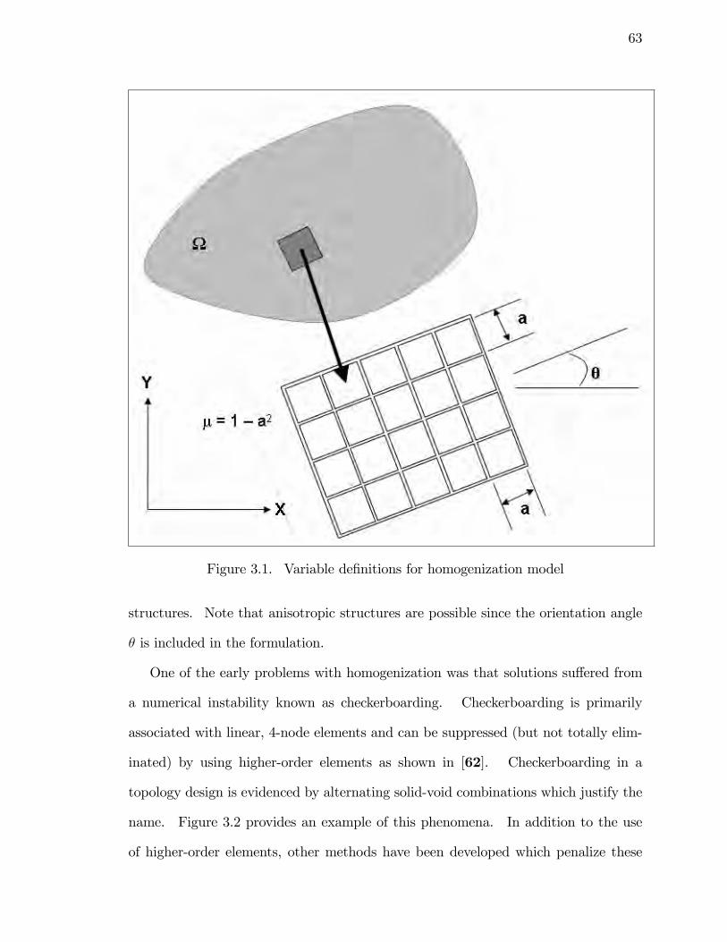
63
Figure 3.1. Variable de�nitions for homogenization model
structures. Note that anisotropic structures are possible since the orientation angle
� is included in the formulation.
One of the early problems with homogenization was that solutions su¤ered from
a numerical instability known as checkerboarding. Checkerboarding is primarily
associated with linear, 4-node elements and can be suppressed (but not totally elim-
inated) by using higher-order elements as shown in [62]. Checkerboarding in a
topology design is evidenced by alternating solid-void combinations which justify the
name. Figure 3.2 provides an example of this phenomena. In addition to the use
of higher-order elements, other methods have been developed which penalize these
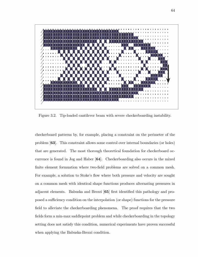
64
Figure 3.2. Tip-loaded cantilever beam with severe checkerboarding instability.
checkerboard patterns by, for example, placing a constraint on the perimeter of the
problem [63]. This constraint allows some control over internal boundaries (or holes)
that are generated. The most thorough theoretical foundation for checkerboard oc-
currence is found in Jog and Haber [64]. Checkerboarding also occurs in the mixed
�nite element formuation where two-�eld problems are solved on a common mesh.
For example, a solution to Stoke�s �ow where both pressure and velocity are sought
on a common mesh with identical shape functions produces alternating pressures in
adjacent elements. Babuska and Brezzi [65] �rst identi�ed this pathology and pro-
posed a su¢ ciency condition on the interpolation (or shape) functions for the pressure
�eld to alleviate the checkerboarding phenomena. The proof requires that the two
�elds form a min-max saddlepoint problem and while checkerboarding in the topology
setting does not satisfy this condition, numerical experiments have proven successful
when applying the Babuska-Brezzi condition.
65
3.3. Solid Isotropic Material with Penalization (SIMP)
Another method which relaxes the �0-1�design space is the "solid isotropic ma-
terial with penalization" (or SIMP) method. One of the primary advantages of the
SIMP method is its conceptual simplicity [66] and [67]. The SIMP method allows
intermediate densities to exist in a domain as opposed to the all or nothing approach
of material or void. In the typical SIMP approach, material properties are assumed
constant within each �nite element used to discretize the design domain (although
this assumption is not essential to the development) with the design variables being
the element "densities". This density �eld variable does not have to represent the
true mass density of the material. Instead it can be a user-de�ned �eld variable that
is used simply as a multiplier to adjust the modulus. The material properties are
modeled to be proportional to the relative density raised to a power. For example,
the fourth-order elasticity tensor is given by Eq. 3.1,
(3.1) Eijkl (x) =
�� (x)
�0 (x)
�pE0ijkl (x)
where Eijkl is the scaled value of the elasticity tensor �eld, E0ijkl is the initial value of
the elasticity tensor, � is the density, �0 is the initial density and p an integer power.
The e¤ect of the exponent p is to penalize intermediate densities (Figure 3.3). Since
intermediate densities are permitted in this method, a penalization of intermediate
densities is necessary to prevent so-called "grey" designs from evolving as they are
not manufacturable from a two-constituent (material or void) model. The problem
with penalizing intermediate densities is that the di¢ culties associated with the �0-1�
problem (e.g., checkerboarding) return as the penalty becomes large. In Figure 3.3,
we can see that as the exponent increases, fewer and fewer intermediate modulus ratio
values are possible. The value of p is typically chosen to be approximately three. To
66
circumvent the problems associated with the �0-1�highly penalized behavior and still
arrive at designs which contain very little intermediate density, the value of p can be
chosen small initially and increased as the optimization proceeds. This approach is
known as a continuation method [68]. The power-law based approach to topology
optimization has been widely applied to problems with multiple constraints, multiple
physics and multiple materials. In fact, all (to the author�s knowledge) commercial
topology optimization codes include a SIMP implementation. This method is chosen
primarily for its ease of implementation into a �nite element framework. However, the
close association of the SIMP topology optimization method with the �nite element
discretization also limits the topologies generated and can cause mesh dependency
issues which much be addressed through �ltering techniques [69], [70] and [71].
3.4. Level Set Method
The most recent technique for addressing the structural topology optimization
problem is known as the level set model. This model combines level set methods [72]
and a mathematical programming method for optimization. The level set method uses
implicit, moving boundaries for topology optimization. The structural boundaries are
viewed as moving during the optimization process. Interior boundaries (or holes) may
merge with each other or with the exterior boundary and new holes may be created.
A level set model speci�es a surface in an implicit form as an iso-surface of a scalar
function, � : R3 �! R, embedded in 3D, i.e.,
(3.2) S = fx : � (x) = kg
where k is the iso-value and is arbitrary, and x is a point in space on the iso-surface
�. x is the set of points in R3 that composes the kth iso-surface of �. The embedded
� can be speci�ed in any speci�c form, e.g., as a regular sampling on a rectilinear
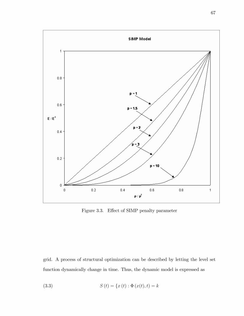
67
Figure 3.3. E¤ect of SIMP penalty parameter
grid. A process of structural optimization can be described by letting the level set
function dynamically change in time. Thus, the dynamic model is expressed as
(3.3) S (t) = fx (t) : � (x(t); t) = k
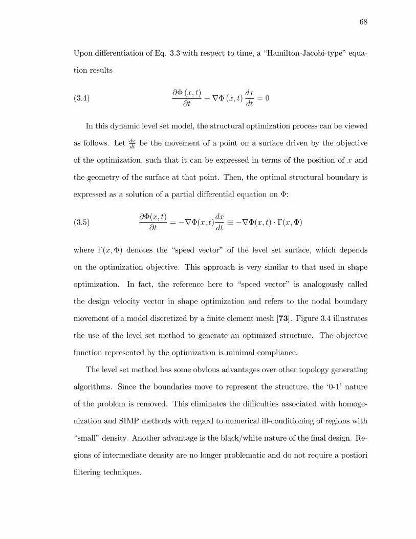
68
Upon di¤erentiation of Eq. 3.3 with respect to time, a �Hamilton-Jacobi-type�equa-
tion results
(3.4)@� (x; t)
@t+r� (x; t) dx
dt= 0
In this dynamic level set model, the structural optimization process can be viewed
as follows. Let dxdtbe the movement of a point on a surface driven by the objective
of the optimization, such that it can be expressed in terms of the position of x and
the geometry of the surface at that point. Then, the optimal structural boundary is
expressed as a solution of a partial di¤erential equation on �:
(3.5)@�(x; t)
@t= �r�(x; t)dx
dt� �r�(x; t) � �(x;�)
where �(x;�) denotes the �speed vector� of the level set surface, which depends
on the optimization objective. This approach is very similar to that used in shape
optimization. In fact, the reference here to �speed vector� is analogously called
the design velocity vector in shape optimization and refers to the nodal boundary
movement of a model discretized by a �nite element mesh [73]. Figure 3.4 illustrates
the use of the level set method to generate an optimized structure. The objective
function represented by the optimization is minimal compliance.
The level set method has some obvious advantages over other topology generating
algorithms. Since the boundaries move to represent the structure, the �0-1�nature
of the problem is removed. This eliminates the di¢ culties associated with homoge-
nization and SIMP methods with regard to numerical ill-conditioning of regions with
�small�density. Another advantage is the black/white nature of the �nal design. Re-
gions of intermediate density are no longer problematic and do not require a postiori
�ltering techniques.
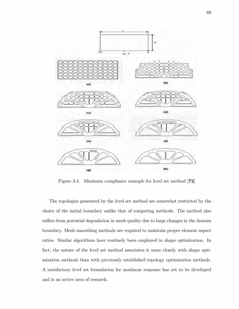
69
Figure 3.4. Minimum compliance example for level set method [72]
The topologies generated by the level set method are somewhat restricted by the
choice of the initial boundary unlike that of competing methods. The method also
su¤ers from potential degradation in mesh quality due to large changes in the domain
boundary. Mesh smoothing methods are required to maintain proper element aspect
ratios. Similar algorithms have routinely been employed in shape optimization. In
fact, the nature of the level set method associates it more closely with shape opti-
mization methods than with previously established topology optimization methods.
A satisfactory level set formulation for nonlinear response has yet to be developed
and is an active area of research.
70
3.5. Evolutionary Structural Optimization (ESO)
The Evolutionary Structural Optimization (ESO) method for topology optimiza-
tion was �rst introduced in 1993 in [74]. The genesis for the method has its origins in
the well-known optimality criteria concept in structural optimization known as �fully-
stressed design.�A fully stressed design (FSD) is de�ned as one in which each point
in the body is fully utilized with respect to stress allowables[75]. In application, the
FSD method usually takes the form of driving the structure toward a uniform stress
state. To accomplish the objective, ine¢ cient material is slowly removed from the
body over many iterations for the given loading. This slow removal of material sub-
stantiates the �evolution�reference in the method title, i.e., the structure �evolves�
toward an �optimal�con�guration.
There are obvious similarities between the SIMP and ESO methods. In the SIMP
method, ine¢ cient material is, in essence, removed by adjusting the modulus down-
ward. In the ESO method, a more discrete methodology is employed which literally
removes the ine¢ cient material. Just as the SIMP method is closely tied to the �-
nite element method with regard to material discretization, so is the ESO method.
Therefore, ine¢ cient elements are removed from the initial structure generating in-
ternal surfaces.
The ESOmethod is similar to the aforementioned methods in that a design domain
is chosen large enough to cover the area of the �nal design. The design domain
is discretized by a �ne mesh of �nite elements. Loads and boundary conditions
are applied and a stress analysis is performed. The stress response is interrogated
comparing the lowly stressed regions to the rest of the structure. An appropriate
rejection criterion is chosen and is used to remove ine¢ cient material, i.e., elements.
An average stress value is computed for each element using the components of the
stress tensor. For this purpose the von Mises stress has been one of the most widely
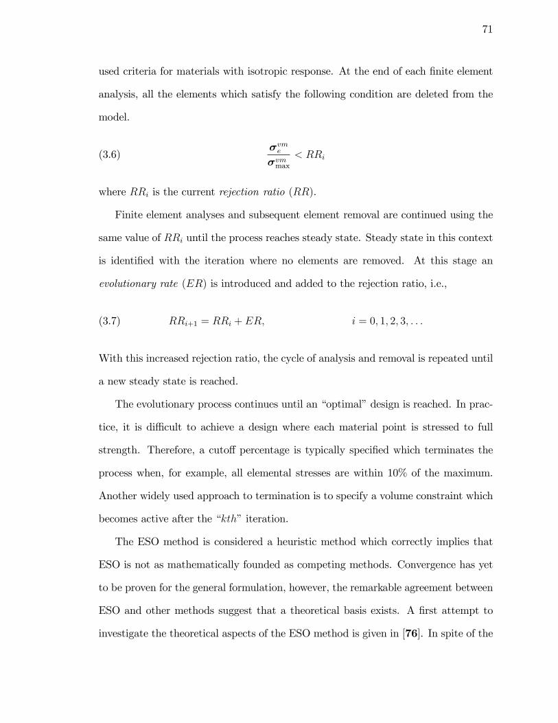
71
used criteria for materials with isotropic response. At the end of each �nite element
analysis, all the elements which satisfy the following condition are deleted from the
model.
(3.6)�vme�vmmax
< RRi
where RRi is the current rejection ratio (RR).
Finite element analyses and subsequent element removal are continued using the
same value of RRi until the process reaches steady state. Steady state in this context
is identi�ed with the iteration where no elements are removed. At this stage an
evolutionary rate (ER) is introduced and added to the rejection ratio, i.e.,
(3.7) RRi+1 = RRi + ER; i = 0; 1; 2; 3; : : :
With this increased rejection ratio, the cycle of analysis and removal is repeated until
a new steady state is reached.
The evolutionary process continues until an �optimal�design is reached. In prac-
tice, it is di¢ cult to achieve a design where each material point is stressed to full
strength. Therefore, a cuto¤ percentage is typically speci�ed which terminates the
process when, for example, all elemental stresses are within 10% of the maximum.
Another widely used approach to termination is to specify a volume constraint which
becomes active after the �kth�iteration.
The ESO method is considered a heuristic method which correctly implies that
ESO is not as mathematically founded as competing methods. Convergence has yet
to be proven for the general formulation, however, the remarkable agreement between
ESO and other methods suggest that a theoretical basis exists. A �rst attempt to
investigate the theoretical aspects of the ESO method is given in [76]. In spite of the
72
infancy of the theoretical foundation, the ease with which the ESO formulation can
be incorporated into a commercial �nite element code makes it a formidable tool for
design optimization.
Checkerboarding does occur in ESO designs similar to highly penalized SIMP
models. A scheme to suppress these unwanted topologies is presented in [77]. The
method replaces the raw elemental stress response from the analysis with an averaged
value based on neighboring element values.
3.6. Formulations
In this section, the formulations for topology optimization applications speci�c
to solid mechanics will be presented. While topology optimization is not limited to
structural applications, the overwhelming majority of work has been in this area.
The scope of this section begins very broadly eventually narrowing to the topic of
nonlinear thermoelastic applications.
3.6.1. Minimum Compliance Design
When a topology optimization problem is formulated, a design objective must be
chosen. A seemingly obvious choice is to minimize volume subject to local stress
constraints on each �nite element. While this objective/constraint combination has
been pursued in the literature, a fully satisfactory, robust formulation has yet to be
accomplished [78]. Having a local stress constraint on each element destroys the
e¢ ciency of the widely used adjoint sensitivity method. The adjoint method can
accomodate a large number of design variables very e¢ ciently, but its advantages are
diminished as the number of response equations increases. Another consideration
when attempting to apply local stress constraints is the limit state value. If we
specify that the von-Mises stress, �kvm, in element k should remain less than some
73
value (e.g, yield stress, �y),
(3.8) �kvm < �y
as the optimization proceeds, the density of each element will undoubtedly change.
The question arises as to what value of �y should be used for these intermediate den-
sities. The so-called "singularity" problem associated with stress constraints requires
special consideration in topology optimization [78]. The design space de�ned by the
constraint equations su¤ers from an "irregularity" that produces degenerated appen-
dices in which the Slater condition does not hold. The result of this pathology renders
algorithms based on Kuhn-Tucker conditions ill-equipped to locate the optima. Mild
success in this area has been achieved by prescribing stress constraints over regions
of the model (groups of elements) which converts the local stress constraints to a
global quantity and renders the design space more amenable to conventional opti-
mization methods. By not being able to address the stress issue directly, there is
no guarantee that an "optimal" topology will be a useful structural design. The
study of stress constraints remains a very active area of research as the solution to
this problem would make the critical connection between topology optimization and
robust structures.
An objective function which does not su¤er from the pathologies of the stress
objective while producing useful structures is given by the compliance. Minimiza-
tion of compliance subject to a volume constraint is the most widely used topology
optimization formulation in literature. For linear elastic structures, the minimum
compliance formulation takes the following form where the objective is to determine
the sti¤ness tensor Eijkl(x) as a �eld variable over the entire domain, . Introducing
74
the energy bilinear form:
(3.9) a (u; v) =
Z
Eijkl (x) "ij (u) "kl (v) d
with linearized strains
(3.10) "ij (u) =1
2
�@ui@xj
+@uj
@xi
�
and the load linear form
(3.11) l(u) =
Z
b u d +
Z�T
t u ds
the minimum compliance or maximum global sti¤ness problem is given by
minu�U;E
l(u)(3.12)
s:t: : aE (u; v) = l(v); for all v � U
The equilibrium equation is expressed in weak form with U denoting the space of
kinematically admissible displacement �elds, b, the body forces and t, the tractions
on the prescribed traction portion of the boundary, �T . The subscript E in the
bilinear form denotes the dependence on the sti¤ness tensor.
If the domain of the bilinear form is discretized into a �nite element mesh with
appropriate basis functions, the familiar �nite element statement of equilibrium is
given by
(3.13) [K] fug = ffg
where [K] is the global sti¤ness matrix, fug is the vector of nodal displacements, and
ffg is the nodal force vector. Also in discretized form, the compliance is the nodal
75
force vector multiplied by the nodal displacements,
(3.14) l(u) = ffgT fug
Combining equations 3.13 and 3.14, the compliance is given by
l(u) = ([K] fug)T fug(3.15)
= fugT [K]T fug(3.16)
The reader familiar with strain energy concepts will recognize equation 3.16 as two
times the strain energy of a linear elastic structure provided the sti¤ness matrix is
symmetric. Therefore, minimization of strain energy ensures minimum compliance
(or maximum sti¤ness) of a linear elastic structure.
3.6.2. Linear Thermoelasticity
The �rst work which addressed the minimum compliance problem for thermoelastic
structures was the journal article by Rodrigues, et. al. [79]. The development
presented in this paper extended the material-based formulation presented by Bend-
søe and Kikuchi [57], to include the e¤ect of temperature di¤erential. The material
e¤ective (homogenized) properties for both the elastic moduli and the thermal expan-
sion coe¢ cient are computed using the homogenization method. The mathematical
statement of the compliance objective is given by
(3.17) min(0 � �(x) � 1; �(x)
�Z
b � u d +Z
�H(�; �)"(u)�T d +
Z�
t � u d��
subjected to the isoperimetric constraint on volume,
(3.18)Z
�(x) d � �V
76
assuming the constitutive law of linear thermoelasticity,
(3.19) � = EH"(u)� �H�T
whereEH(�; �) is the homogenized fourth-order elasticity tensor, �H(�; �) the second-
order, diagonal, homogenized thermal expansion coe¢ cient tensor, �H(�; �) = EH(�; �)�H(�; �),
and u is the solution of the equilibrium equation, in weak form,
Z
EH(�; �)"(u)"(w)� �H(�; �)"(u)�T � b � u d�Z�
t � u d� = 0;(3.20)
8 w admissible
The equations in this section are combined into a single Lagrangian equation which
facilitates the derivation of the optimality conditions. These equations are then
solved numerically to arrive at optimal topologies.
It should be noticed that for structural problems in thermoelasticity, the work
done by the loads includes the contribution from the thermal expansion terms (Eq.
3.17) and is explicitly dependent on the design via the thermal property tensor, �H .
One implication of this compliance de�nition is, as the temperature increases, the
optimal structure may fail to use all available material, (i.e., the volume constraint
will be inactive). Rodriguez, et. al. demonstrates this fact with a combined thermo-
mechanically loaded two-dimensional example problem. The inital design domain
(Figure 3.5) and the resulting topologies are shown for a constant mechanical loading
and �T = 0 (Figure 3.6) and �T = 1� using 4-noded elements (Figure 3.7). The
results of using higher-order elements (9-noded) are are shown in Figure 3.8. In
the �gures below, the darker areas indicate �xed regions. For the mechanical-only
loading, the volume constraint is active providing the most material to resist the
displacement in the direction of loading. In Figure 3.7 we see that supports are
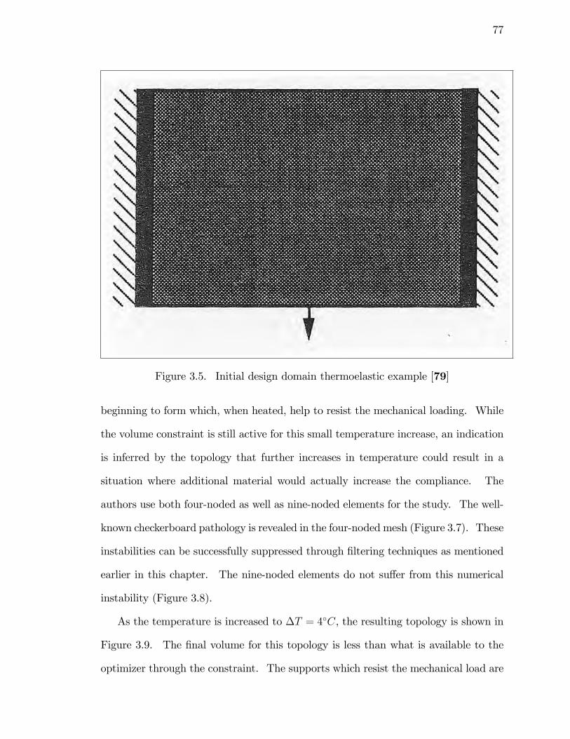
77
Figure 3.5. Initial design domain thermoelastic example [79]
beginning to form which, when heated, help to resist the mechanical loading. While
the volume constraint is still active for this small temperature increase, an indication
is inferred by the topology that further increases in temperature could result in a
situation where additional material would actually increase the compliance. The
authors use both four-noded as well as nine-noded elements for the study. The well-
known checkerboard pathology is revealed in the four-noded mesh (Figure 3.7). These
instabilities can be successfully suppressed through �ltering techniques as mentioned
earlier in this chapter. The nine-noded elements do not su¤er from this numerical
instability (Figure 3.8).
As the temperature is increased to �T = 4�C, the resulting topology is shown in
Figure 3.9. The �nal volume for this topology is less than what is available to the
optimizer through the constraint. The supports which resist the mechanical load are
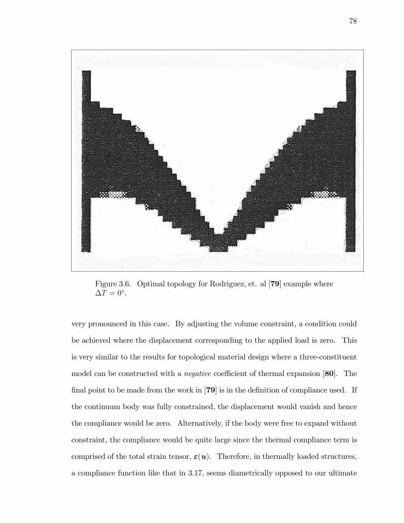
78
Figure 3.6. Optimal topology for Rodriguez, et. al [79] example where�T = 0�.
very pronounced in this case. By adjusting the volume constraint, a condition could
be achieved where the displacement corresponding to the applied load is zero. This
is very similar to the results for topological material design where a three-constituent
model can be constructed with a negative coe¢ cient of thermal expansion [80]. The
�nal point to be made from the work in [79] is in the de�nition of compliance used. If
the continuum body was fully constrained, the displacement would vanish and hence
the compliance would be zero. Alternatively, if the body were free to expand without
constraint, the compliance would be quite large since the thermal compliance term is
comprised of the total strain tensor, "(u). Therefore, in thermally loaded structures,
a compliance function like that in 3.17, seems diametrically opposed to our ultimate
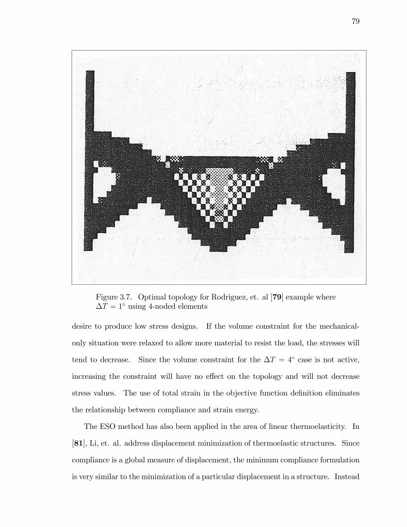
79
Figure 3.7. Optimal topology for Rodriguez, et. al [79] example where�T = 1� using 4-noded elements
desire to produce low stress designs. If the volume constraint for the mechanical-
only situation were relaxed to allow more material to resist the load, the stresses will
tend to decrease. Since the volume constraint for the �T = 4� case is not active,
increasing the constraint will have no e¤ect on the topology and will not decrease
stress values. The use of total strain in the objective function de�nition eliminates
the relationship between compliance and strain energy.
The ESO method has also been applied in the area of linear thermoelasticity. In
[81], Li, et. al. address displacement minimization of thermoelastic structures. Since
compliance is a global measure of displacement, the minimum compliance formulation
is very similar to the minimization of a particular displacement in a structure. Instead
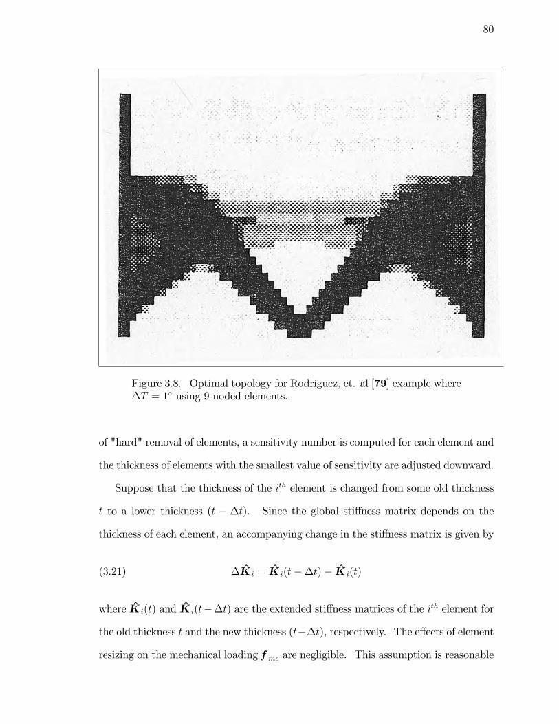
80
Figure 3.8. Optimal topology for Rodriguez, et. al [79] example where�T = 1� using 9-noded elements.
of "hard" removal of elements, a sensitivity number is computed for each element and
the thickness of elements with the smallest value of sensitivity are adjusted downward.
Suppose that the thickness of the ith element is changed from some old thickness
t to a lower thickness (t � �t). Since the global sti¤ness matrix depends on the
thickness of each element, an accompanying change in the sti¤ness matrix is given by
(3.21) �K̂i = K̂i(t��t)� K̂i(t)
where K̂i(t) and K̂i(t��t) are the extended sti¤ness matrices of the ith element for
the old thickness t and the new thickness (t��t), respectively. The e¤ects of element
resizing on the mechanical loading fme are negligible. This assumption is reasonable
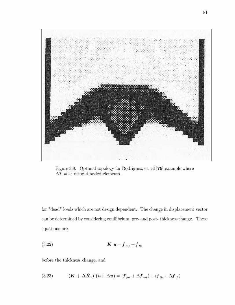
81
Figure 3.9. Optimal topology for Rodriguez, et. al [79] example where�T = 4� using 4-noded elements.
for "dead" loads which are not design dependent. The change in displacement vector
can be determined by considering equilibrium, pre- and post- thickness change. These
equations are
(3.22) K u = fme + f th
before the thickness change, and
(3.23) (K +�K̂i) (u+ �u) = (fme +�fme) + (f th +�f th)
82
after the thickness change where fme and f th denote the mechanical and thermal
loads, �fme(= 0) and �f th denote the changes in mechanical and thermal loads,
respectively. By subtracting Eq. 3.22 from Eq. 3.23 and ignoring higher order
terms, the �rst order change in displacement vector is given by
(3.24) �u = K�1(�f th ��K̂iu)
To �nd the change in a given jth displacement component uj, a virtual mechanical
load vector f j is introduced, in which the jth component is equal to one and all others
are equal to zero. Taking the scalar product of Eq. 3.24 with the transpose of f j, the
change �uj in the speci�ed jth displacement component due to the thickness change
in the ith element is determined as
�uj = fTj ��u = fTj �K�1(�f th ��K̂iu)(3.25)
= uTj ��f th � uTj ��K̂i u
where uj is the displacement solution of the virtual system K u = f j. The reader
familiar with the adjoint sensitivity method will see the similarity between the "vir-
tual" load and the pseudo-load of the adjoint approach. Since Eq. 3.25 is a scalar
value, the calculations may be computed at the element level. For the ith element,
(3.26) �uj = uTij ��f i;th � uTj ��Ki ui
where �Ki denotes the change in element sti¤ness matrix due to its respective thick-
ness change, ui and uij represent, respectively, the entries from global solution vectors
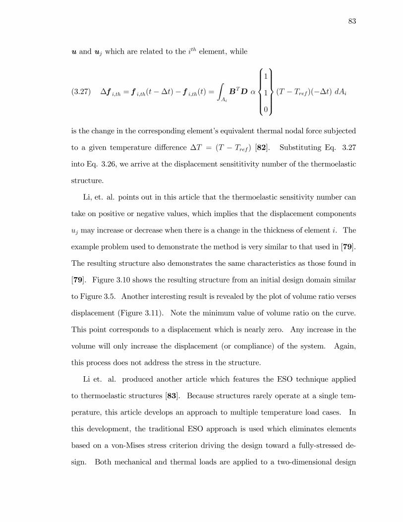
83
u and uj which are related to the ith element, while
(3.27) �f i;th = f i;th(t��t)� f i;th(t) =ZAi
BTD �
8>>>><>>>>:1
1
0
9>>>>=>>>>; (T � Tref )(��t) dAi
is the change in the corresponding element�s equivalent thermal nodal force subjected
to a given temperature di¤erence �T = (T � Tref ) [82]. Substituting Eq. 3.27
into Eq. 3.26, we arrive at the displacement sensititivity number of the thermoelastic
structure.
Li, et. al. points out in this article that the thermoelastic sensitivity number can
take on positive or negative values, which implies that the displacement components
uj may increase or decrease when there is a change in the thickness of element i. The
example problem used to demonstrate the method is very similar to that used in [79].
The resulting structure also demonstrates the same characteristics as those found in
[79]. Figure 3.10 shows the resulting structure from an initial design domain similar
to Figure 3.5. Another interesting result is revealed by the plot of volume ratio verses
displacement (Figure 3.11). Note the minimum value of volume ratio on the curve.
This point corresponds to a displacement which is nearly zero. Any increase in the
volume will only increase the displacement (or compliance) of the system. Again,
this process does not address the stress in the structure.
Li et. al. produced another article which features the ESO technique applied
to thermoelastic structures [83]. Because structures rarely operate at a single tem-
perature, this article develops an approach to multiple temperature load cases. In
this development, the traditional ESO approach is used which eliminates elements
based on a von-Mises stress criterion driving the design toward a fully-stressed de-
sign. Both mechanical and thermal loads are applied to a two-dimensional design
84
Figure 3.10. Optimized thickness design for displacement minimization(V/Vo=54.7%) [81].
Figure 3.11. Evolution history of displacement vs volume ratio [81].
85
domain, again similar to that used in [79]. The structures generated are also very
similar to the optimized shapes found in the minimum compliance designs of [79].
This is not surprising as the equivalence between the ESO stress criterion and mini-
mum compliance was established in [84]. The concept of fully-stressed design should
not be confused with necessarily producing low stressed designs. Removing lowly
stressed elements does produce e¢ cient designs where very little underutilized mate-
rial remains. However, as material is removed from a mechanically-loaded structure,
the stress will typically increase as a simple appeal to � = P=A; with diminishing A;
reveals. The fact that the temperature load takes the form of a design dependency
is not mentioned in the article. No consideration in the objective function is given
to the fact that thermal stress will be relieved if expansion is allowed.
3.6.3. Nonlinear Thermoelasticity
Linear elasticity has been, by far, the area to which topology optimization has been
most applied. This formulation makes up the foundation of virtually all commercially
available topology codes. The obvious reason for this focus is the relative infancy of
the topology method when compared with other optimization techniques. So as not
to convolute the results of the various topology methods, the simplest response was
chosen, i.e., linear elasticity, as the demonstration tool.
More recent developments have moved beyond the linear elastic model and have
addressed the topology optimization of nonlinear elastic structures [71] and [85]. In
[71], Bruns and Tortorelli solve the minimum compliance objective with a volume
constraint for small strain but allow for large displacement. The authors compare
the results from both linear and nonlinear topology optimization. Their �ndings
indicate that while the compliances between the two approaches were similar, the
resulting topologies were di¤erent.
86
The �rst work to address nonlinear thermoelasticity was by Jog [86]. Jog�s for-
mulation is similar to the SIMP method in which a "density" variable is introduced to
transform the problem from one of integer programming to a continuous variable over
the domain. The variable is penalized to remove intermediate densities. Jog also
introduces a perimeter constraint to eliminate the tendency toward checkerboarding.
Jog makes very precise de�nitions of the equations of motion and energy. These
strong forms of the equations are reproduced from earlier work in linear thermoelas-
ticity [87]. Jog also generalizes the compliance de�nition given in [79]. His topology
optimization statement combines the compliance of the mechanical loading and the
thermal loading through a simple additive equation. Jog, similar to Rodriguez et. al.
[79], uses the total strain, (albeit the Green�s strain due to the nonlinear formulation),
to de�ne the thermal compliance contribution. He summizes that this objective will
not lead necessarily to lower stress designs due to the non-proportionality between
stress and strain. The author concludes that, under combined thermo-mechanical
loading, a di¤erent performance functional would have to be used in order to have a
more even (magnitude-wise) stress distribution in the structure.
3.6.4. Coupled Heat Transfer and Minimum Compliance
Up to this point, we have examined topology optimizations where the temperature
�eld has been treated as a known or given distribution that is independent of the
topology changes that take place. In many real life scenarios, a heat �ux may
be prescribed on a boundary along with convection and radiation conditions also
prescribed on various portions of the domain. Therefore, only a small number of cases
lend themselves to treating the temperature �eld as independent of the topology with
the primary exception being that of uniform temperature. As the topology changes,
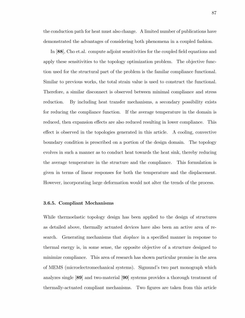
87
the conduction path for heat must also change. A limited number of publications have
demonstrated the advantages of considering both phenomena in a coupled fashion.
In [88], Cho et.al. compute adjoint sensitivities for the coupled �eld equations and
apply these sensitivities to the topology optimization problem. The objective func-
tion used for the structural part of the problem is the familar compliance functional.
Similar to previous works, the total strain value is used to construct the functional.
Therefore, a similar disconnect is observed between minimal compliance and stress
reduction. By including heat transfer mechanisms, a secondary possibility exists
for reducing the compliance function. If the average temperature in the domain is
reduced, then expansion e¤ects are also reduced resulting in lower compliance. This
e¤ect is observed in the topologies generated in this article. A cooling, convective
boundary condition is prescribed on a portion of the design domain. The topology
evolves in such a manner as to conduct heat towards the heat sink, thereby reducing
the average temperature in the structure and the compliance. This formulation is
given in terms of linear responses for both the temperature and the displacement.
However, incorporating large deformation would not alter the trends of the process.
3.6.5. Compliant Mechanisms
While thermoelastic topology design has been applied to the design of structures
as detailed above, thermally actuated devices have also been an active area of re-
search. Generating mechanisms that displace in a speci�ed manner in response to
thermal energy is, in some sense, the opposite objective of a structure designed to
minimize compliance. This area of research has shown particular promise in the area
of MEMS (microelectromechanical systems). Sigmund�s two part monograph which
analyzes single [89] and two-material [90] systems provides a thorough treatment of
thermally-actuated compliant mechanisms. Two �gures are taken from this article
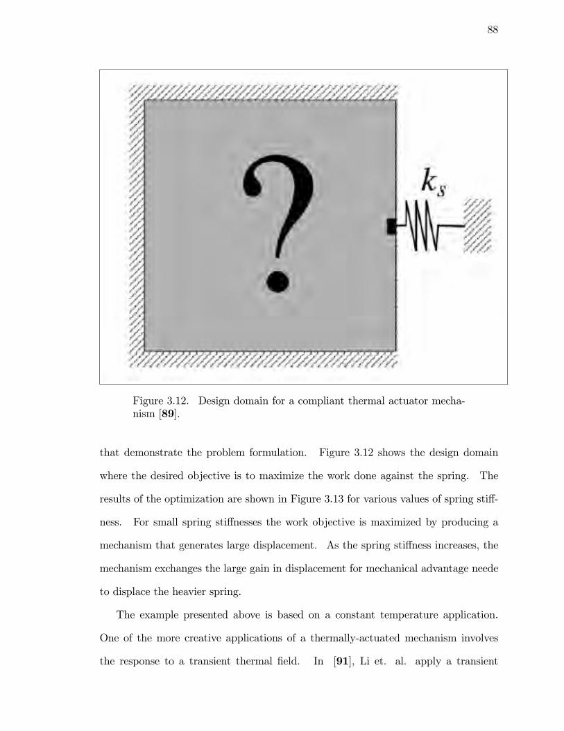
88
Figure 3.12. Design domain for a compliant thermal actuator mecha-nism [89].
that demonstrate the problem formulation. Figure 3.12 shows the design domain
where the desired objective is to maximize the work done against the spring. The
results of the optimization are shown in Figure 3.13 for various values of spring sti¤-
ness. For small spring sti¤nesses the work objective is maximized by producing a
mechanism that generates large displacement. As the spring sti¤ness increases, the
mechanism exchanges the large gain in displacement for mechanical advantage neede
to displace the heavier spring.
The example presented above is based on a constant temperature application.
One of the more creative applications of a thermally-actuated mechanism involves
the response to a transient thermal �eld. In [91], Li et. al. apply a transient
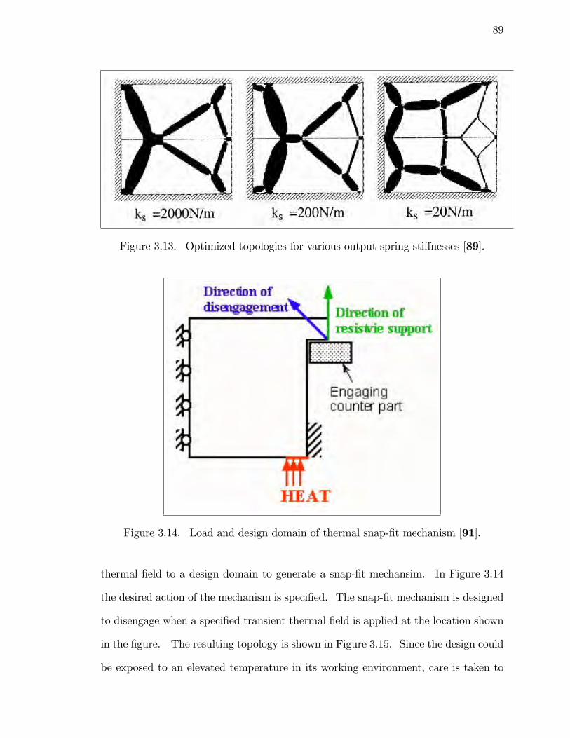
89
Figure 3.13. Optimized topologies for various output spring sti¤nesses [89].
Figure 3.14. Load and design domain of thermal snap-�t mechanism [91].
thermal �eld to a design domain to generate a snap-�t mechansim. In Figure 3.14
the desired action of the mechanism is speci�ed. The snap-�t mechanism is designed
to disengage when a speci�ed transient thermal �eld is applied at the location shown
in the �gure. The resulting topology is shown in Figure 3.15. Since the design could
be exposed to an elevated temperature in its working environment, care is taken to
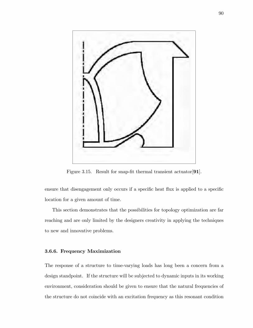
90
Figure 3.15. Result for snap-�t thermal transient actuator[91].
ensure that disengagement only occurs if a speci�c heat �ux is applied to a speci�c
location for a given amount of time.
This section demonstrates that the possibilities for topology optimization are far
reaching and are only limited by the designers creativity in applying the techniques
to new and innovative problems.
3.6.6. Frequency Maximization
The response of a structure to time-varying loads has long been a concern from a
design standpoint. If the structure will be subjected to dynamic inputs in its working
environment, consideration should be given to ensure that the natural frequencies of
the structure do not coincide with an excitation frequency as this resonant condition
91
can result in large amplitude oscillations. Topology optimization, with its inherent
capability for design variation, is ideally suited for frequency optimization. The
problem formulation takes the following form (Eq. 3.28)
max�
(�min = min�i
i=1;:::;Ndof
)(3.28)
s:t: : (K � �iM) �i = 0; i = 1; : : : ; Ndof
NXe=1
ve�e � V; 0 < �min � �e � 1; e = 1; : : : N
whereK andM represent the sti¤ness and mass matrices, respectively and �i is the
eigenvector associated with ith eigenvalue. In practice, only the �rst few modes are
of interest (~10) in determining the dynamic response. One important observation
with regard to the frequency optimization problem (Eq. 3.28) is the existence of a
trivial solution. As stated, (Eq. 3.28) will attain an in�nite frequency by removing
the entire structure. Hence, the eigenvalue formulation is primarily used to reinforce
an existing structure with regions that are �xed (or non-designable) due to other
problem constraints.
Homogenization, SIMP and ESO have all been successfully applied to frequency
optimization. One di¢ culty that arises when the optimizer is attemping to drive a
freqency to a target value is the phenomena known as mode-switching [54]. This
phenomena manifests itself when (as the name implies) a mode shape that was orig-
inally associated with a large eigenvalue exchanges with an initially low frequency
mode shape. This phenomena causes problems for the optimizer as the active con-
straint can be switching at each iteration. Variants of the formulation have been
developed which place an additional constraint on eigenvalue separation to eliminate
the problematic condition from occuring [92].
92
3.7. Summary
The intent of this chapter was to provide the reader with enough information to
appreciate previous e¤orts in topology optimization of thermo-elastic structures. The
body of work in this area is relatively sparse as most topological designs address the
mechanically-loaded situation. We have shown the most common objective function,
compliance, is not a good objective when attempting to sti¤en structure that is failing
due to thermally-induced loads. A satisfying approach which can sti¤en curved or
�at panels without unduly supplying load to the boundary has yet to be developed.
In the next chapter an approach to this end is proposed.
CHAPTER 4
SIMP Approach to Sti¤ening of Thermally-Loaded Curved
Shells
4.1. Introduction
In this chapter a simple but e¤ective procedure for developing topology designs in
constrained thermal environments will be presented. As was demonstrated in Chapter
2, the trade space that develops when attempting to alleviate high edge stresses in
thermally-loaded shallow shells is one of tensile stress reduction verses increased load
into supporting structure. A conventional approach to failures resulting from out-of-
plane bending would appear to require the addition of structural members with large
moments of inertia. Typical structural members of this variety include I- or T-shaped
beams. In a loading scenario in which the loads are independent of the structure, this
approach has proven successful in many applications. However, when the loading
becomes dependent on the structure, as is the case in a thermal environment, the
e¤ect of the sti¤ener on the load must be considered.
Stresses in thin, thermally-loaded shells result primarily from the inhibition of
thermal expansion. Due to the skin�s inability to expand su¢ ciently against the sti¤
boundaries, out-of-plane deformation results either through buckling (for a �at plate)
or through bowing in the case of an initially curved panel. Two approaches can be
taken to diminish the tensile stresses in the panel. The �rst approach involves the
addition of sti¤eners large enough to provide motion at the sti¤ boundaries. This
approach essentially forces expansion of the boundary creating additional space for
the expansion of the skin with little or no resistance. Structural members designed
93
94
for bending are not necessary since the primary load being carried is compression
(provided buckling is inhibited). In this scenario, the skin will be virtually load and
stress free. The newly-added structural members support the load and the thin skin
simply follows the large stuctural members as they expand. The di¢ culty with this
approach is obtaining accurate information regarding the sti¤ness of the boundary.
As was demonstrated in Chapter 2, the additional force resulting from sti¤ening the
skin varies widely depending on the boundary sti¤ness. If model inaccuracies and
assumptions predict a softer boundary than actually exist in the structure, loads
into the boundary as well as stresses in the sti¤ened shell will be underpredicted.
If the structure is placed back in service, failures in adjacent structure and/or the
original panel could result. So while this approach can produce satisfactory designs,
it requires a high level of �delity in the model. A model to produce this level of
predictive capability would require experimental validation of the boundary sti¤nesses
at each location where the skin is attached to sub- and surrounding structure.
The second approach and the one followed in this work is to provide just enough
out-of-plane sti¤ening to enable the skin to carry greater compressive load without
resorting to excessive out-of-plane deformation. Since the material will be placed in
such a manner as to prohibit only transverse de�ection, a minimal increase in load is
expected from the expansion of the additional, sti¤ening structure. As was demon-
strated in Chapter 3, the minimum compliance topology formulation for structures
whose primary loads are due to thermal expansion does not ensure lower stresses as
the volume constraint is relaxed. While this behavior is intuitive and observed in
structures whose function is to support mechanical loads, increasing volume in a ther-
mal stress problem can actually increase compliance. And since thermal expansion
e¤ects are related to the volume of the material, as volume increases so too does the
potential for larger stresses and reaction loads. To circumvent the problematic issues
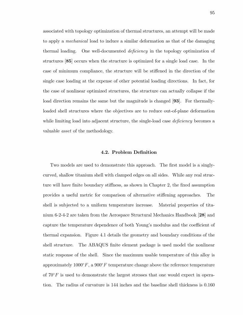
95
associated with topology optimization of thermal structures, an attempt will be made
to apply a mechanical load to induce a similar deformation as that of the damaging
thermal loading. One well-documented de�ciency in the topology optimization of
structures [85] occurs when the structure is optimized for a single load case. In the
case of minimum compliance, the structure will be sti¤ened in the direction of the
single case loading at the expense of other potential loading directions. In fact, for
the case of nonlinear optimized structures, the structure can actually collapse if the
load direction remains the same but the magnitude is changed [93]. For thermally-
loaded shell structures where the objectives are to reduce out-of-plane deformation
while limiting load into adjacent structure, the single-load case de�ciency becomes a
valuable asset of the methodology.
4.2. Problem De�nition
Two models are used to demonstrate this approach. The �rst model is a singly-
curved, shallow titanium shell with clamped edges on all sides. While any real struc-
ture will have �nite boundary sti¤ness, as shown in Chapter 2, the �xed assumption
provides a useful metric for comparison of alternative sti¤ening approaches. The
shell is subjected to a uniform temperature increase. Material properties of tita-
nium 6-2-4-2 are taken from the Aerospace Structural Mechanics Handbook [28] and
capture the temperature dependence of both Young�s modulus and the coe¢ cient of
thermal expansion. Figure 4.1 details the geometry and boundary conditions of the
shell structure. The ABAQUS �nite element package is used model the nonlinear
static response of the shell. Since the maximum usable temperature of this alloy is
approximately 1000�F , a 900�F temperature change above the reference temperature
of 70�F is used to demonstrate the largest stresses that one would expect in opera-
tion. The radius of curvature is 144 inches and the baseline shell thickness is 0.160
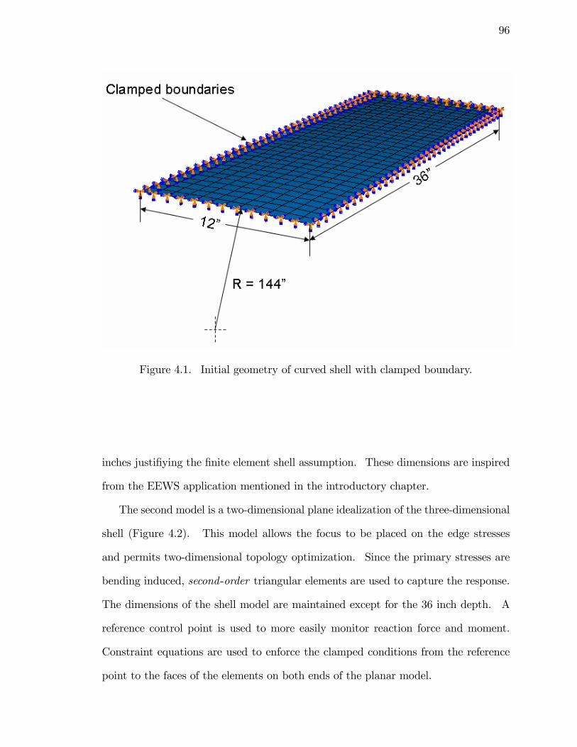
96
Figure 4.1. Initial geometry of curved shell with clamped boundary.
inches justi�ying the �nite element shell assumption. These dimensions are inspired
from the EEWS application mentioned in the introductory chapter.
The second model is a two-dimensional plane idealization of the three-dimensional
shell (Figure 4.2). This model allows the focus to be placed on the edge stresses
and permits two-dimensional topology optimization. Since the primary stresses are
bending induced, second-order triangular elements are used to capture the response.
The dimensions of the shell model are maintained except for the 36 inch depth. A
reference control point is used to more easily monitor reaction force and moment.
Constraint equations are used to enforce the clamped conditions from the reference
point to the faces of the elements on both ends of the planar model.
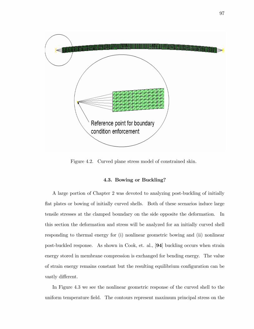
97
Figure 4.2. Curved plane stress model of constrained skin.
4.3. Bowing or Buckling?
A large portion of Chapter 2 was devoted to analyzing post-buckling of initially
�at plates or bowing of initially curved shells. Both of these scenarios induce large
tensile stresses at the clamped boundary on the side opposite the deformation. In
this section the deformation and stress will be analyzed for an initially curved shell
responding to thermal energy for (i) nonlinear geometric bowing and (ii) nonlinear
post-buckled response. As shown in Cook, et. al., [94] buckling occurs when strain
energy stored in membrane compression is exchanged for bending energy. The value
of strain energy remains constant but the resulting equilibrium con�guration can be
vastly di¤erent.
In Figure 4.3 we see the nonlinear geometric response of the curved shell to the
uniform temperature �eld. The contours represent maximum principal stress on the
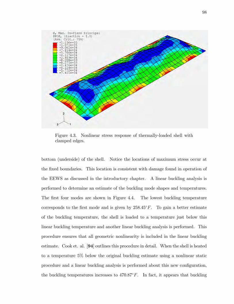
98
Figure 4.3. Nonlinear stress response of thermally-loaded shell withclamped edges.
bottom (underside) of the shell. Notice the locations of maximum stress occur at
the �xed boundaries. This location is consistent with damage found in operation of
the EEWS as discussed in the introductory chapter. A linear buckling analysis is
performed to determine an estimate of the buckling mode shapes and temperatures.
The �rst four modes are shown in Figure 4.4. The lowest buckling temperature
corresponds to the �rst mode and is given by 258.45�F . To gain a better estimate
of the buckling temperature, the shell is loaded to a temperature just below this
linear buckling temperature and another linear buckling analysis is performed. This
procedure ensures that all geometric nonlinearity is included in the linear buckling
estimate. Cook et. al. [94] outlines this procedure in detail. When the shell is heated
to a temperature 5% below the original buckling estimate using a nonlinear static
procedure and a linear buckling analysis is performed about this new con�guration,
the buckling temperatures increases to 470.87�F . In fact, it appears that buckling
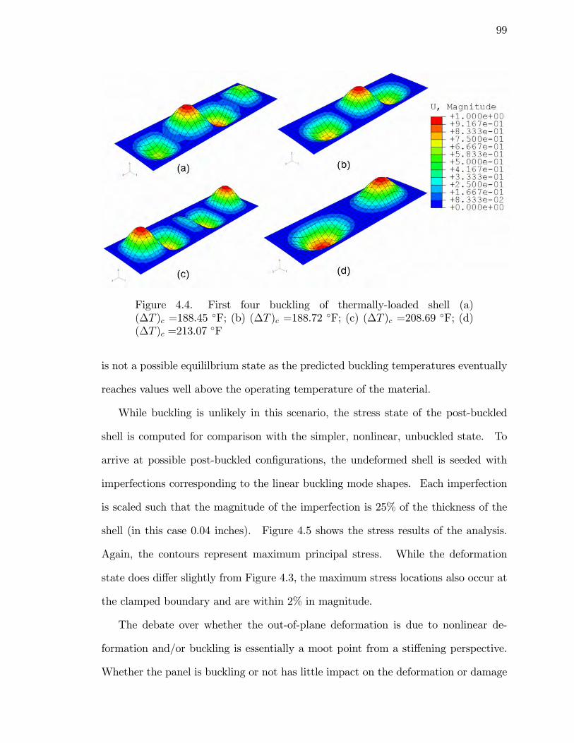
99
Figure 4.4. First four buckling of thermally-loaded shell (a)(�T )c =188.45 �F; (b) (�T )c =188.72 �F; (c) (�T )c =208.69 �F; (d)(�T )c =213.07 �F
is not a possible equililbrium state as the predicted buckling temperatures eventually
reaches values well above the operating temperature of the material.
While buckling is unlikely in this scenario, the stress state of the post-buckled
shell is computed for comparison with the simpler, nonlinear, unbuckled state. To
arrive at possible post-buckled con�gurations, the undeformed shell is seeded with
imperfections corresponding to the linear buckling mode shapes. Each imperfection
is scaled such that the magnitude of the imperfection is 25% of the thickness of the
shell (in this case 0.04 inches). Figure 4.5 shows the stress results of the analysis.
Again, the contours represent maximum principal stress. While the deformation
state does di¤er slightly from Figure 4.3, the maximum stress locations also occur at
the clamped boundary and are within 2% in magnitude.
The debate over whether the out-of-plane deformation is due to nonlinear de-
formation and/or buckling is essentially a moot point from a sti¤ening perspective.
Whether the panel is buckling or not has little impact on the deformation or damage
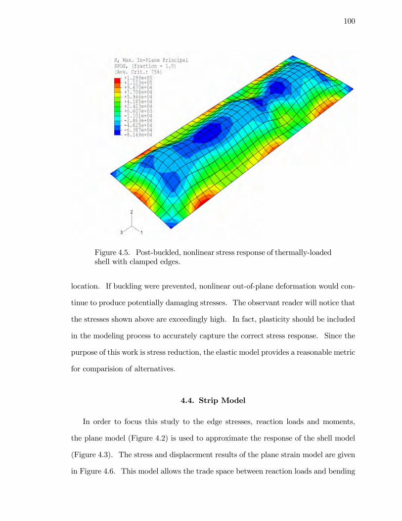
100
Figure 4.5. Post-buckled, nonlinear stress response of thermally-loadedshell with clamped edges.
location. If buckling were prevented, nonlinear out-of-plane deformation would con-
tinue to produce potentially damaging stresses. The observant reader will notice that
the stresses shown above are exceedingly high. In fact, plasticity should be included
in the modeling process to accurately capture the correct stress response. Since the
purpose of this work is stress reduction, the elastic model provides a reasonable metric
for comparision of alternatives.
4.4. Strip Model
In order to focus this study to the edge stresses, reaction loads and moments,
the plane model (Figure 4.2) is used to approximate the response of the shell model
(Figure 4.3). The stress and displacement results of the plane strain model are given
in Figure 4.6. This model allows the trade space between reaction loads and bending
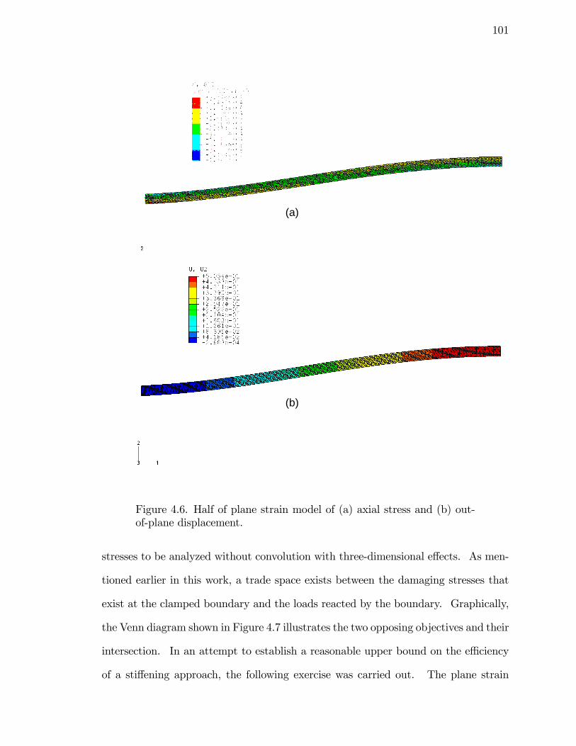
101
(a)
(b)
(a)(a)
(b)
Figure 4.6. Half of plane strain model of (a) axial stress and (b) out-of-plane displacement.
stresses to be analyzed without convolution with three-dimensional e¤ects. As men-
tioned earlier in this work, a trade space exists between the damaging stresses that
exist at the clamped boundary and the loads reacted by the boundary. Graphically,
the Venn diagram shown in Figure 4.7 illustrates the two opposing objectives and their
intersection. In an attempt to establish a reasonable upper bound on the e¢ ciency
of a sti¤ening approach, the following exercise was carried out. The plane strain
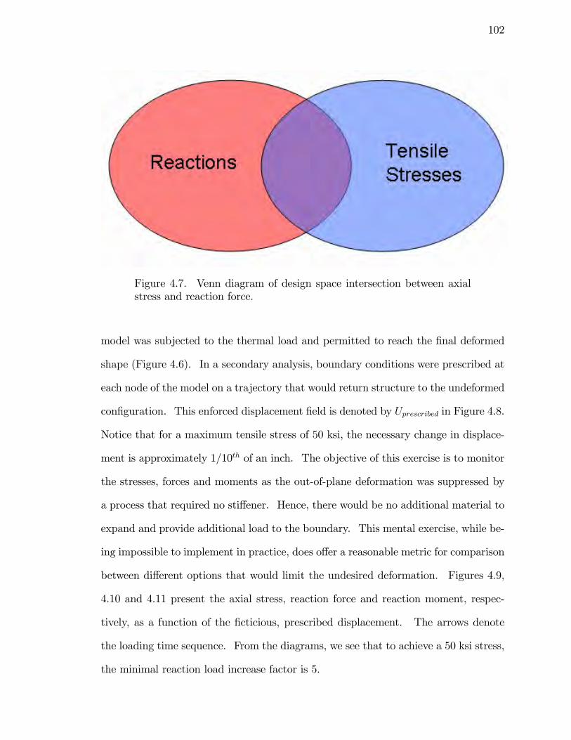
102
Figure 4.7. Venn diagram of design space intersection between axialstress and reaction force.
model was subjected to the thermal load and permitted to reach the �nal deformed
shape (Figure 4.6). In a secondary analysis, boundary conditions were prescribed at
each node of the model on a trajectory that would return structure to the undeformed
con�guration. This enforced displacement �eld is denoted by Uprescribed in Figure 4.8.
Notice that for a maximum tensile stress of 50 ksi, the necessary change in displace-
ment is approximately 1/10th of an inch. The objective of this exercise is to monitor
the stresses, forces and moments as the out-of-plane deformation was suppressed by
a process that required no sti¤ener. Hence, there would be no additional material to
expand and provide additional load to the boundary. This mental exercise, while be-
ing impossible to implement in practice, does o¤er a reasonable metric for comparison
between di¤erent options that would limit the undesired deformation. Figures 4.9,
4.10 and 4.11 present the axial stress, reaction force and reaction moment, respec-
tively, as a function of the �cticious, prescribed displacement. The arrows denote
the loading time sequence. From the diagrams, we see that to achieve a 50 ksi stress,
the minimal reaction load increase factor is 5.
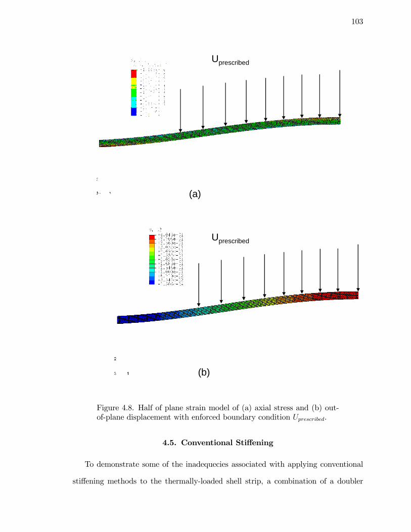
103
(a)
Uprescribed
(b)
Uprescribed
(a)
Uprescribed
(a)
Uprescribed
(b)
Uprescribed
(b)
Uprescribed
Figure 4.8. Half of plane strain model of (a) axial stress and (b) out-of-plane displacement with enforced boundary condition Uprescribed.
4.5. Conventional Sti¤ening
To demonstrate some of the inadequecies associated with applying conventional
sti¤ening methods to the thermally-loaded shell strip, a combination of a doubler
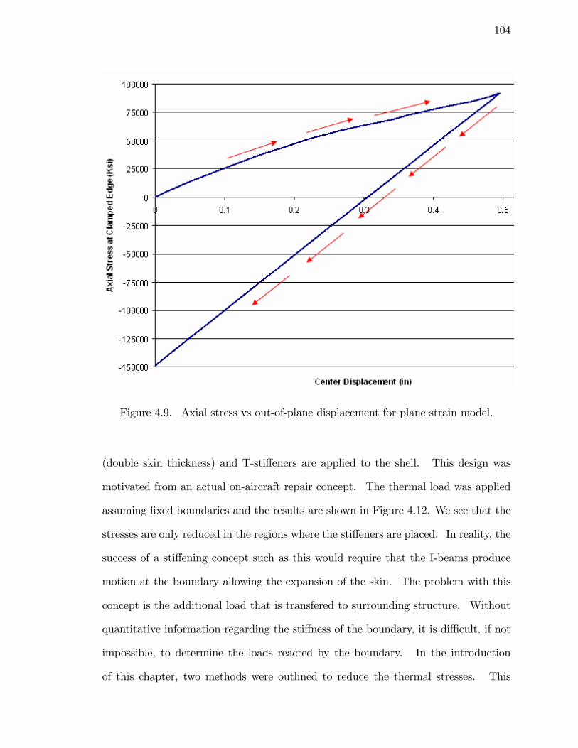
104
Figure 4.9. Axial stress vs out-of-plane displacement for plane strain model.
(double skin thickness) and T-sti¤eners are applied to the shell. This design was
motivated from an actual on-aircraft repair concept. The thermal load was applied
assuming �xed boundaries and the results are shown in Figure 4.12. We see that the
stresses are only reduced in the regions where the sti¤eners are placed. In reality, the
success of a sti¤ening concept such as this would require that the I-beams produce
motion at the boundary allowing the expansion of the skin. The problem with this
concept is the additional load that is transfered to surrounding structure. Without
quantitative information regarding the sti¤ness of the boundary, it is di¢ cult, if not
impossible, to determine the loads reacted by the boundary. In the introduction
of this chapter, two methods were outlined to reduce the thermal stresses. This
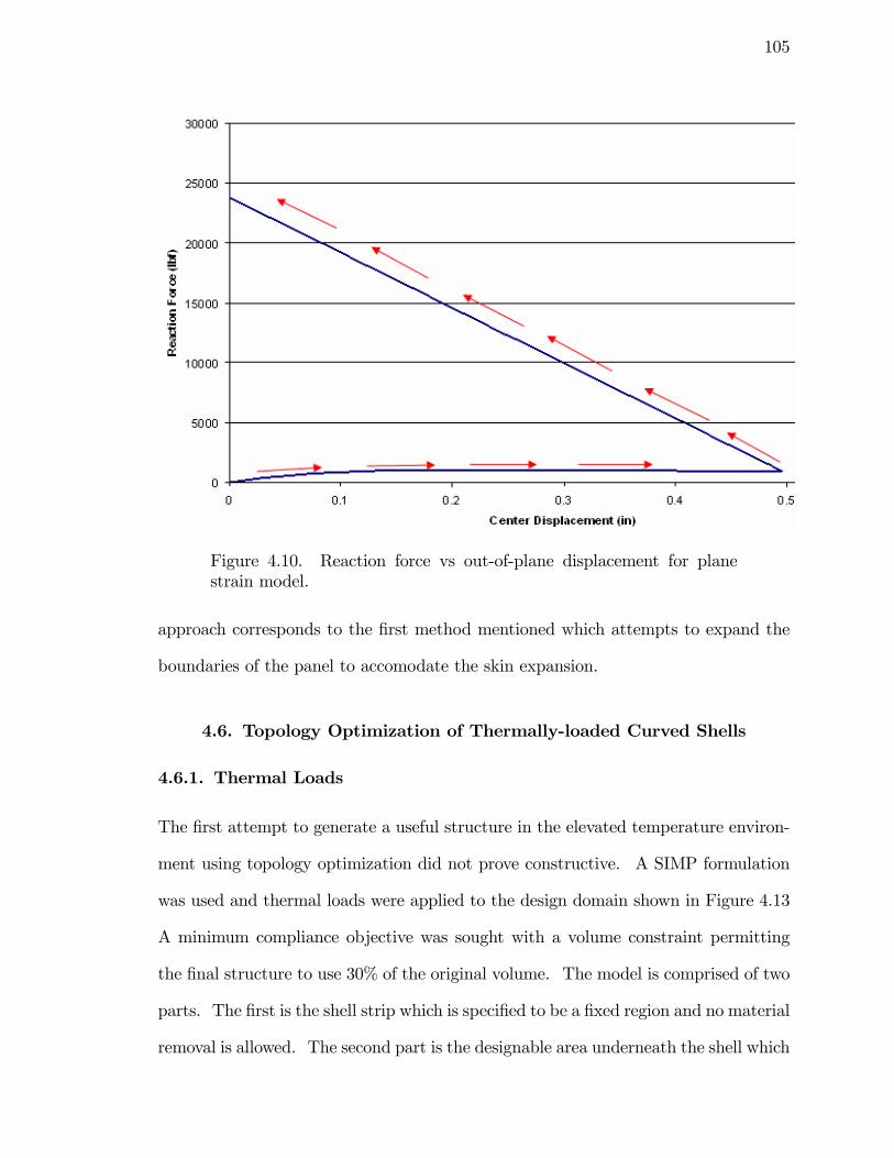
105
Figure 4.10. Reaction force vs out-of-plane displacement for planestrain model.
approach corresponds to the �rst method mentioned which attempts to expand the
boundaries of the panel to accomodate the skin expansion.
4.6. Topology Optimization of Thermally-loaded Curved Shells
4.6.1. Thermal Loads
The �rst attempt to generate a useful structure in the elevated temperature environ-
ment using topology optimization did not prove constructive. A SIMP formulation
was used and thermal loads were applied to the design domain shown in Figure 4.13
A minimum compliance objective was sought with a volume constraint permitting
the �nal structure to use 30% of the original volume. The model is comprised of two
parts. The �rst is the shell strip which is speci�ed to be a �xed region and no material
removal is allowed. The second part is the designable area underneath the shell which
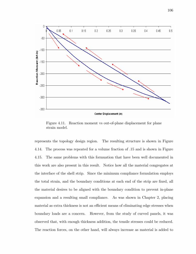
106
Figure 4.11. Reaction moment vs out-of-plane displacement for planestrain model.
represents the topology design region. The resulting structure is shown in Figure
4.14. The process was repeated for a volume fraction of .15 and is shown in Figure
4.15. The same problems with this formuation that have been well documented in
this work are also present in this result. Notice how all the material congregates at
the interface of the shell strip. Since the minimum compliance formulation employs
the total strain, and the boundary conditions at each end of the strip are �xed, all
the material desires to be aligned with the boundary condition to prevent in-plane
expansion and a resulting small compliance. As was shown in Chapter 2, placing
material as extra thickness is not an e¢ cient means of eliminating edge stresses when
boundary loads are a concern. However, from the study of curved panels, it was
observed that, with enough thickness addition, the tensile stresses could be reduced.
The reaction forces, on the other hand, will always increase as material is added to
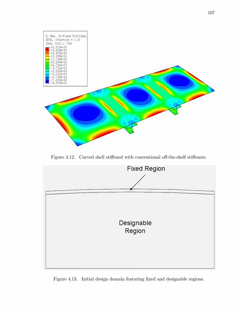
107
Figure 4.12. Curved shell sti¤ened with conventional o¤-the-shelf sti¤eners.
Figure 4.13. Initial design domain featuring �xed and designable regions.
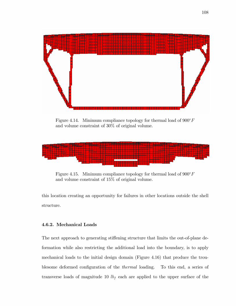
108
Figure 4.14. Minimum compliance topology for thermal load of 900�Fand volume constraint of 30% of original volume.
Figure 4.15. Minimum compliance topology for thermal load of 900�Fand volume constraint of 15% of original volume.
this location creating an opportunity for failures in other locations outside the shell
structure.
4.6.2. Mechanical Loads
The next approach to generating sti¤ening structure that limits the out-of-plane de-
formation while also restricting the additional load into the boundary, is to apply
mechanical loads to the initial design domain (Figure 4.16) that produce the trou-
blesome deformed con�guration of the thermal loading. To this end, a series of
transverse loads of magnitude 10 lbf each are applied to the upper surface of the
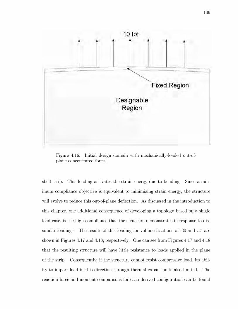
109
Figure 4.16. Initial design domain with mechanically-loaded out-of-plane concentrated forces.
shell strip. This loading activates the strain energy due to bending. Since a min-
imum compliance objective is equivalent to minimizing strain energy, the structure
will evolve to reduce this out-of-plane de�ection. As discussed in the introduction to
this chapter, one additional consequence of developing a topology based on a single
load case, is the high compliance that the structure demonstrates in response to dis-
similar loadings. The results of this loading for volume fractions of .30 and .15 are
shown in Figures 4.17 and 4.18, respectively. One can see from Figures 4.17 and 4.18
that the resulting structure will have little resistance to loads applied in the plane
of the strip. Consequently, if the structure cannot resist compressive load, its abil-
ity to impart load in this direction through thermal expansion is also limited. The
reaction force and moment comparisons for each derived con�guration can be found
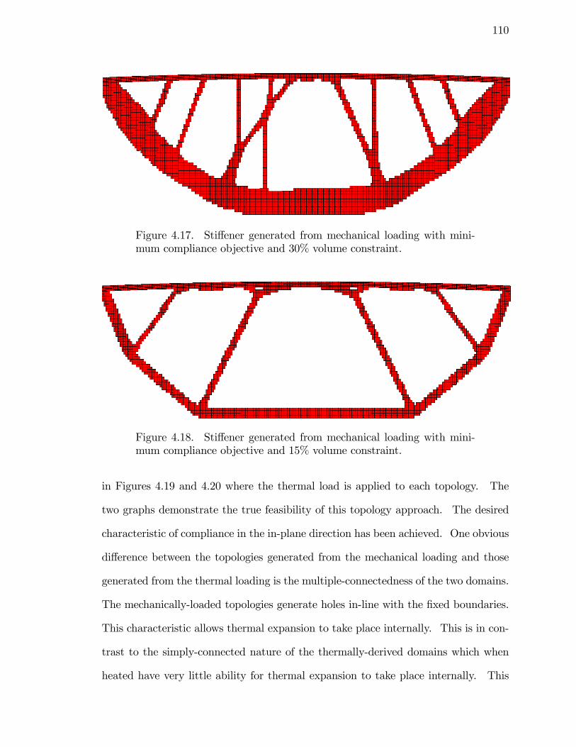
110
Figure 4.17. Sti¤ener generated from mechanical loading with mini-mum compliance objective and 30% volume constraint.
Figure 4.18. Sti¤ener generated from mechanical loading with mini-mum compliance objective and 15% volume constraint.
in Figures 4.19 and 4.20 where the thermal load is applied to each topology. The
two graphs demonstrate the true feasibility of this topology approach. The desired
characteristic of compliance in the in-plane direction has been achieved. One obvious
di¤erence between the topologies generated from the mechanical loading and those
generated from the thermal loading is the multiple-connectedness of the two domains.
The mechanically-loaded topologies generate holes in-line with the �xed boundaries.
This characteristic allows thermal expansion to take place internally. This is in con-
trast to the simply-connected nature of the thermally-derived domains which when
heated have very little ability for thermal expansion to take place internally. This
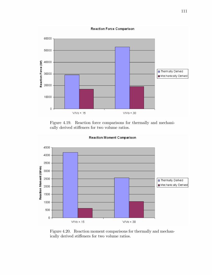
111
Figure 4.19. Reaction force comparisons for thermally and mechani-cally derived sti¤eners for two volume ratios.
Figure 4.20. Reaction moment comparisons for thermally and mechan-ically derived sti¤eners for two volume ratios.
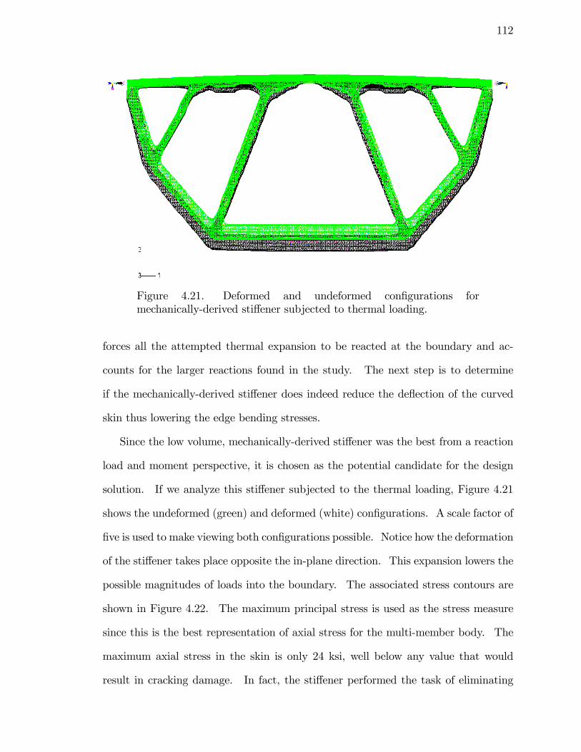
112
Figure 4.21. Deformed and undeformed con�gurations formechanically-derived sti¤ener subjected to thermal loading.
forces all the attempted thermal expansion to be reacted at the boundary and ac-
counts for the larger reactions found in the study. The next step is to determine
if the mechanically-derived sti¤ener does indeed reduce the de�ection of the curved
skin thus lowering the edge bending stresses.
Since the low volume, mechanically-derived sti¤ener was the best from a reaction
load and moment perspective, it is chosen as the potential candidate for the design
solution. If we analyze this sti¤ener subjected to the thermal loading, Figure 4.21
shows the undeformed (green) and deformed (white) con�gurations. A scale factor of
�ve is used to make viewing both con�gurations possible. Notice how the deformation
of the sti¤ener takes place opposite the in-plane direction. This expansion lowers the
possible magnitudes of loads into the boundary. The associated stress contours are
shown in Figure 4.22. The maximum principal stress is used as the stress measure
since this is the best representation of axial stress for the multi-member body. The
maximum axial stress in the skin is only 24 ksi, well below any value that would
result in cracking damage. In fact, the sti¤ener performed the task of eliminating

113
Figure 4.22. Principal stress contours for mechanically-derivedsti¤ener-skin combination.
out-of-plane deformation so well that the thicknesses of the support structure could
be reduced to allow more de�ection and less load and/or moment reaction. If we
compare the axial stress in the skin with the prescribed displacement lower bound
of the previous section, we see that the to obtain this value of axial stress would
result in a reaction force of 7800 lbf . The reaction force in the mechanically-derived
sti¤ener is 13,400 lbf which results in a factor of 1.72. The moment reaction of
the mechanically-derived sti¤ener is 612 in-lbf while the lower bound is given by 225
in-lbf , a factor of 2.27. When compared with the thermally-derived sti¤ener, these
values seem very reasonable. In fact, the thermally-derived sti¤ener resembles most
conventional sti¤ening methods. For example the addition of a doubler sheet and an
I-beam reacts similarly to this type of approach.
114
4.7. Conclusions
In this chapter, a simple method for developing structure which can be used to
sti¤en a curved shell in a thermally-loaded environment was developed. While the
treatment of topology optimization codes is lacking with respect to thermal loadings,
all commercial topology codes can be employed to derive a structure that will perform
well in a thermal environment. By applying mechanical loads in the problematic
direction, structures are evolved which have the property of compliance in dissimilar
loading directions. When sti¤ening a thermally-loaded shell structure that is failing
prematurely, the �rst and most important objective is to do no harm. By generating a
family of designs that, by their construction, limit the load into surrounding structure,
this objective is accomplished.
The methodology presented in this section could obviously be improved through
shape and/or sizing optimization. An objective which attempts to minimize a least
squares error between the desired displacement of the skin and the displacement
resulting from the optimization could be tailored to produce even more optimal solu-
tions. With topology establishing the property connectivity, many, more traditional
approaches are possible. Another concept which could be employed to amplify the
pull-down e¤ect of the sti¤ener is material grading. If, for example, a two material
system were permitted, one consisting of titanium (low CTE) and another consisting
of Inconel (high CTE), the response of the sti¤ener could be tailored to produce the
desired displacement of the skin. Topology optimization will continue to be an active
area of reasearch as it pertains to thermally-loaded structures.
CHAPTER 5
Multi-objective Evolutionary Structural Optimization Using
Combined Static/Dynamic Control Parameters for Design of
Thermal Protection Systems
In the previous chapter the focus was on a very particular geometry (i.e., curved,
clamped shells). In this chapter, a general three-dimensional domain is chosen to
demonstrate the applicability of topology optimization methods to a generic thermal
protection system. Exterior thermal protection systems (TPS) are responsible for
protecting a spacecraft�s structural components from degradation due to elevated
temperatures that result from atomospheric e¤ects that accompany re-entry. The
requirements for a successful thermal protection system should involve a prescription
for maximum thermal stress as well as minimum natural frequency. During launch
conditions, tremendous vibrational loads are generated from engine noise as a result of
multi-stage to orbit propulsion systems as anyone who has attended a space shuttle
launch can attest. Unlike typical vibration suppression approaches where care is
taken to ensure that the fundamental frequency of the structure is lower or higher
than the loading frequency, to alleviate damaging cycles in an acoustic environment,
a lower bound on frequency must be speci�ed. The content of the noise contains
multiple frequencies and is referred to as wide-band random noise. Typical ranges
for frequency are 0 to 2000 Hz. However, for excitation frequencies above 1000
Hz, the strain levels are small enough that damage accumulation is not a major
concern. Due to a transient temperature pro�le and discrete attachments, thermal
stress is also a concern. Thus in the design of TPS, both maximum thermal stress
115
116
and minimum natural frequency should be considered due to the combined thermo-
acoustic environment inherent in high-speed vehicles. In this work, a multi-objective
structural optimization method for three-dimensional acreage TPS design is developed
using an Evolutionary Structural Optimization (ESO) algorithm. A static control
parameter, employed to �nd the optimum in minimum thermal stress design (in the
von-Mises sense), is modi�ed to simultaneously address the irregular mode-switching
phenomenon, as well as improvement in the modal sti¤ness in dynamic analysis. Two
objectives are optimized simultaneously; namely, the maximization of fundamental
natural frequency and the minimization of maximum thermal stress. The proposed
modi�ed control parameter is demonstrated on the design of a metallic TPS using the
method of weighted objectives. The results are then compared with the conventional
ESO sensitivity approach. This work concludes by applying the methodology which
makes use of both topology and shape optimization in the design of an acreage TPS.
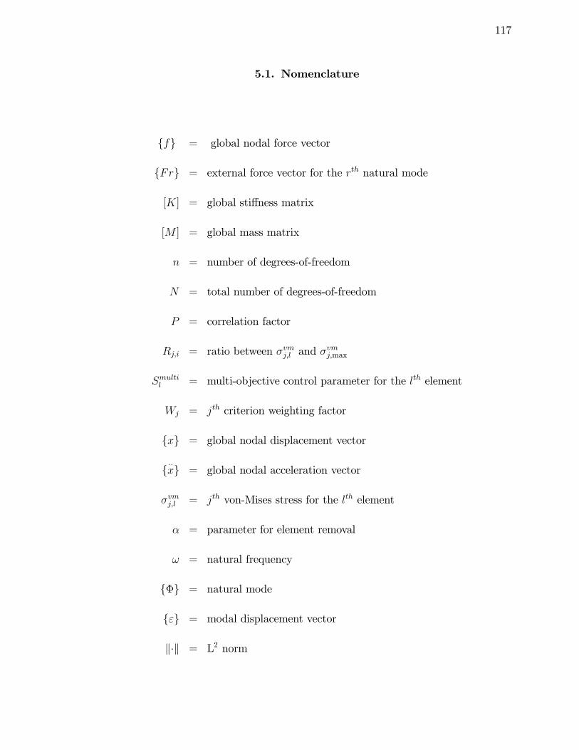
117
5.1. Nomenclature
ffg = global nodal force vector
fFrg = external force vector for the rth natural mode
[K] = global sti¤ness matrix
[M ] = global mass matrix
n = number of degrees-of-freedom
N = total number of degrees-of-freedom
P = correlation factor
Rj;i = ratio between �vmj;l and �vmj;max
Smultil = multi-objective control parameter for the lth element
Wj = jth criterion weighting factor
fxg = global nodal displacement vector
f ��xg = global nodal acceleration vector
�vmj;l = jth von-Mises stress for the lth element
� = parameter for element removal
! = natural frequency
f�g = natural mode
f"g = modal displacement vector
k�k = L2 norm
118
5.2. Introduction
The primary challenges that must be addressed to enable lower-cost access to
space are weight, reusability, and ease of maintenance. The current methodology
for the design of space and high speed air vehicles is to construct a low-temperature
load bearing structure and then apply a thermal protective layer (also known as a
Thermal Protection System (TPS)) whose sole purpose is to shield the low temper-
ature structure. A successful TPS will not only perform its primary function of
maintaining the underlying vehicle structure within acceptable temperature limits,
but must also be durable, operable, cost e¤ective, and lightweight. By construction,
TPS is parasitic with respect to weight. In many situations, the themal insulation
layer is added after the vehicle is sized for structural loads. Typically, the insulation
is attached in such a manner as to permit thermal expansion. When following this
"loose" attachment approach, care must be taken ensure that the random noise from
the engines does not excessively excite the thermal protection system. Current re-
search e¤orts in �hot�structures have investigated the feasibility of using advanced
structural material systems that can function as load bearing structure at elevated
temperature. While hot structures will be important in the future for space and
high-speed air vehicle applications, parasitic TPS remains an enabling technology for
many current applications particularly in the area of re-entry where the heat load is
entirely transient. This work represents a hybrid approach in-between a true "hot"
structure where �ight load and stagnation pressures are reacted as internal loads and
a purely, parasitic TPS where all thermal stress is relieved by expansion joints. In
this work, no attempt is made to apply external �ight loads to the thermal protec-
tion system, however, thermal stresses will result as a "hard" attachment approach
is investigated. By attaching the TPS directly to the low-temperature substructure,
satisfaction of the frequency constraint will be more easily attainable.
119
Existing thermal protection systems consist of various types of materials distrib-
uted over the spacecraft. Thermal insulators used as TPS are comprised of many
material systems including felt blankets, ceramic blankets and tiles, carbon-carbon
leading edges, as well as high temperature metallics. Metallic TPS has some ob-
vious advantages along with several disadvantages. On the plus side, the nature
and response of metals is well understood. Furthermore, the durability and fracture
toughness of metals are typically much greater than that of ceramics. Two important
disadvantages of metallic systems are weight and temperature capability. This work
attempts to mitigate the weight penalty through minimization.
Metallic thermal protection systems for spacecraft operating in an extreme thermal-
acoustic environment is of signi�cant importance [95]. Design considerations for ther-
mal and acoustic loading conditions tend to be diametrically opposed to one another.
So called �oating or compliant designs tend to reduce thermal stresses, whereas sti¤er
designs increase natural frequency and are not as easily excited by wide-band ran-
dom engine noise. To address the TPS design e¢ ciently, optimization methods are
essential from both the standpoint of identifying a potentially small feasible region
as well as driving toward low weight designs.
Traditional structural topology optimization methods, such as the density-based
method, [66], the Homogenization method [57] and [96], and the Evolutionary Struc-
tural Optimization (ESO) method [54] and [97] are applicable to multi-objective op-
timization of static or dynamic (modal) problems. A meaningful multi-objective op-
timization formulation is composed of con�icting objectives in which a compromised,
"best" solution is sought. Hence, multi-objective optimization is the generation of
designs that achieve optimal performance with consideration given to multiple crite-
ria [98] and [99]. Optimization solutions of this nature are known as Pareto optima
120
[99] and [100]. Pareto optima do not produce unique solutions, but rather families
of solutions [101].
The formulation presented in this chapter incorporates a multi-objective optimiza-
tion formulation into the traditional ESO algorithm using the weighted objectives
technique. The ESO method developed by Xie and Steven is based on the princi-
pal that slow removal of ine¢ cient material from a structure evolves the structure
toward an optimum [54]. The ESO procedure addresses the �0-1�problem described
in Chapter 3 more directly than other topology methods. The relaxation that is uti-
lized to render the �0-1�problem well-posed is the small number of elements that are
removed at each iteration. While no proof currently exists, intuitively, the element
removal process in the ESO method can be thought of analogously with the continu-
ation methods used in the SIMP topology approach. Recalling from Chapter 3 that
continuation is achieved by slowly increasing the penalty exponent to approximate
the �0-1�problem at the end of the optimization process.
Traditional ESO procedures do not address the mode-switching phenomenon that
is common in three-dimensional dynamic problems. Mode-switching is a phenomenon
whereby the ordering of natural modes is altered along with structural modi�cation.
The phenomenon often occurs between the natural mode of interest and the neighbor-
ing, orthogonal natural modes. The natural frequency of interest and the modal sti¤-
ness are drastically a¤ected, resulting in convergence di¢ culties and/or non-optimal
con�gurations. In two-dimensional structures, Xie and his colleagues achieved suc-
cess in preventing this pathology by maintaining a prescribed separation between
frequencies [102]. This method, however, is not applicable to three-dimensional
structures in which the phenomenon occurs unpredictably during design iterations.
In addition, as the number of elements eliminated becomes large relative to the initial
design domain, a sudden drop in the natural frequency of interest is observed. This
121
is a direct result of the modal sti¤ness decrease associated with the current level of
element removal. The ESO method and the associated dynamic sensitivity number
[54] fail to consider modal sti¤ness directly. Consequently, these problems make it
harder for the ESO method to determine the Pareto optimum in the multi-objective
optimization [97] that contains dynamic characteristics.
In the next section, control parameters for static and dynamic analysis based on
von-Mises stress are formulated. Section 4 presents the details of the multi-objective
optimization technique. The evolutionary optimization algorithm is described in
Section 5. In section 6, two relevant metallic TPS models with di¤erent load cases
are presented to demonstrate the applicability of the ESO method with the novel
control parameter.
5.3. Sensitivity Analysis
Like most structural optimization methods, many iterations are required for con-
vergence and the ESO procedure is no exception. Therefore, it is important that the
element removal process be e¢ cient and accurate so that the objective is obtained
as quickly as possible. In this section, two control parameters (called sensitivity
numbers [54]), both of which are based on static analyses, are proposed as requisites
for element removal. The static control parameter follows the typical ESO approach,
whereas the modi�ed static control parameter is newly developed and address the
shortcomings of modal sti¤ness reduction and mode-switching phenomenon in nat-
ural frequency optimization.
5.3.1. Control parameter for Static Analysis
To avoid direct consideration of each component of the stress tensor, an average stress
value is assigned to each element. The most common stress measure for this purpose
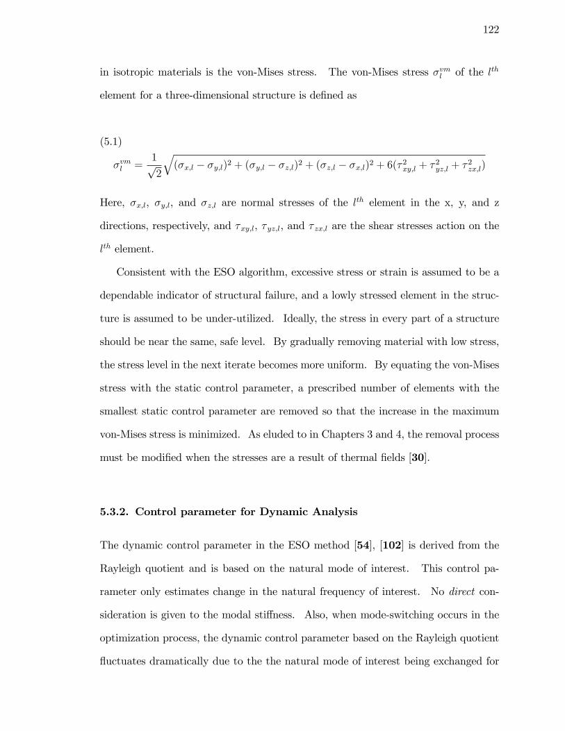
122
in isotropic materials is the von-Mises stress. The von-Mises stress �vml of the lth
element for a three-dimensional structure is de�ned as
(5.1)
�vml =1p2
q(�x;l � �y;l)2 + (�y;l � �z;l)2 + (�z;l � �x;l)2 + 6(� 2xy;l + � 2yz;l + � 2zx;l)
Here, �x;l, �y;l, and �z;l are normal stresses of the lth element in the x, y, and z
directions, respectively, and �xy;l, � yz;l, and � zx;l are the shear stresses action on the
lth element.
Consistent with the ESO algorithm, excessive stress or strain is assumed to be a
dependable indicator of structural failure, and a lowly stressed element in the struc-
ture is assumed to be under-utilized. Ideally, the stress in every part of a structure
should be near the same, safe level. By gradually removing material with low stress,
the stress level in the next iterate becomes more uniform. By equating the von-Mises
stress with the static control parameter, a prescribed number of elements with the
smallest static control parameter are removed so that the increase in the maximum
von-Mises stress is minimized. As eluded to in Chapters 3 and 4, the removal process
must be modi�ed when the stresses are a result of thermal �elds [30].
5.3.2. Control parameter for Dynamic Analysis
The dynamic control parameter in the ESO method [54], [102] is derived from the
Rayleigh quotient and is based on the natural mode of interest. This control pa-
rameter only estimates change in the natural frequency of interest. No direct con-
sideration is given to the modal sti¤ness. Also, when mode-switching occurs in the
optimization process, the dynamic control parameter based on the Rayleigh quotient
�uctuates dramatically due to the the natural mode of interest being exchanged for
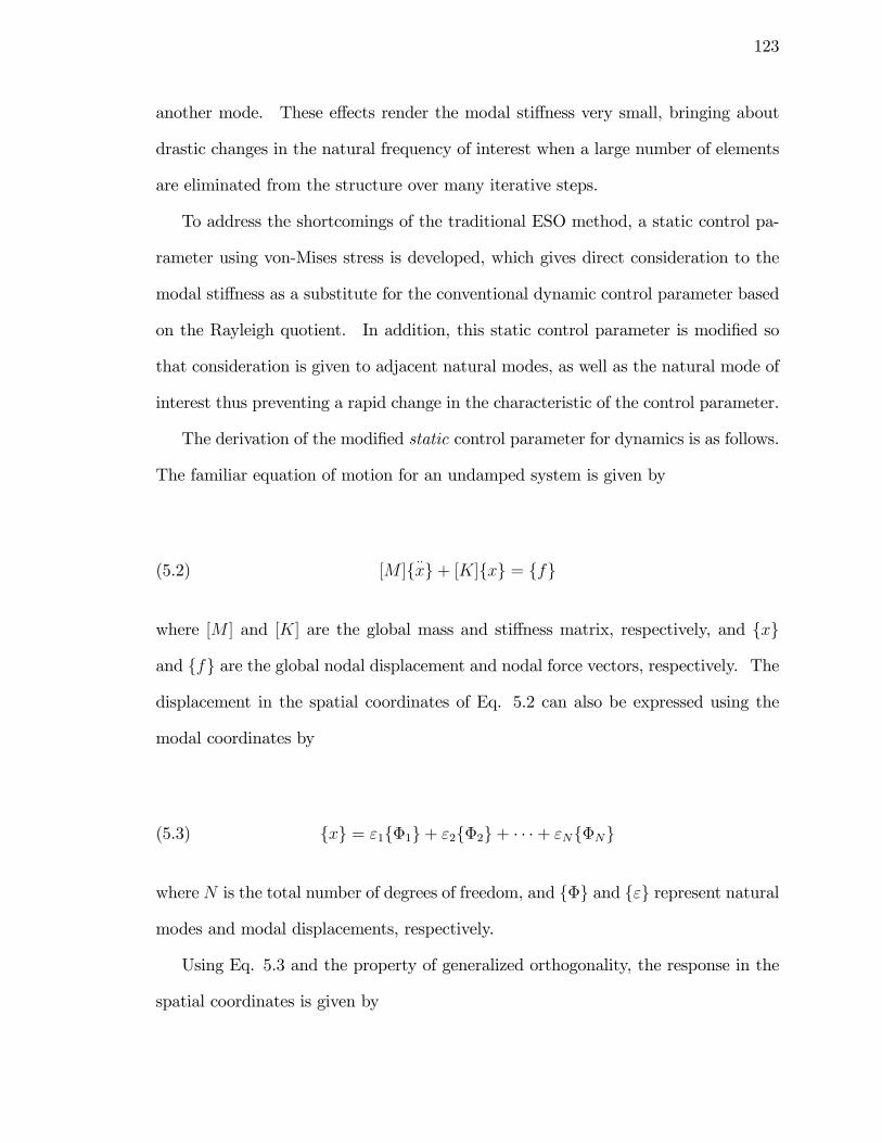
123
another mode. These e¤ects render the modal sti¤ness very small, bringing about
drastic changes in the natural frequency of interest when a large number of elements
are eliminated from the structure over many iterative steps.
To address the shortcomings of the traditional ESO method, a static control pa-
rameter using von-Mises stress is developed, which gives direct consideration to the
modal sti¤ness as a substitute for the conventional dynamic control parameter based
on the Rayleigh quotient. In addition, this static control parameter is modi�ed so
that consideration is given to adjacent natural modes, as well as the natural mode of
interest thus preventing a rapid change in the characteristic of the control parameter.
The derivation of the modi�ed static control parameter for dynamics is as follows.
The familiar equation of motion for an undamped system is given by
(5.2) [M ]f ��xg+ [K]fxg = ffg
where [M ] and [K] are the global mass and sti¤ness matrix, respectively, and fxg
and ffg are the global nodal displacement and nodal force vectors, respectively. The
displacement in the spatial coordinates of Eq. 5.2 can also be expressed using the
modal coordinates by
(5.3) fxg = "1f�1g+ "2f�2g+ � � �+ "Nf�Ng
where N is the total number of degrees of freedom, and f�g and f"g represent natural
modes and modal displacements, respectively.
Using Eq. 5.3 and the property of generalized orthogonality, the response in the
spatial coordinates is given by
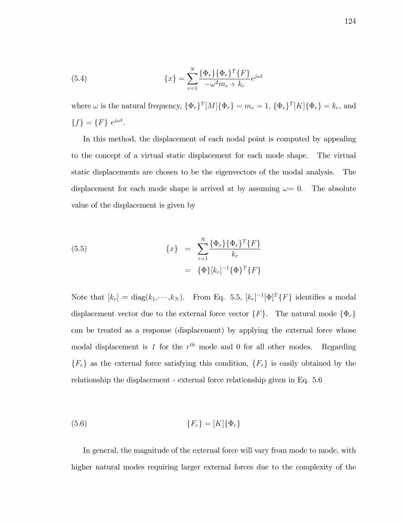
124
(5.4) fxg =NXr=1
f�rgf�rgTfFg�!2mr + kr
ej!t
where ! is the natural frequency, f�rgT [M ]f�rg = mr = 1; f�rgT [K]f�rg = kr, and
ffg = fFg ej!t.
In this method, the displacement of each nodal point is computed by appealing
to the concept of a virtual static displacement for each mode shape. The virtual
static displacements are chosen to be the eigenvectors of the modal analysis. The
displacement for each mode shape is arrived at by assuming != 0. The absolute
value of the displacement is given by
fxg =NXr=1
f�rgf�rgTfFgkr
(5.5)
= f�g[kr]�1f�gTfFg
Note that [kr] = diag(k1,� � � ,kN). From Eq. 5.5, [kr]�1[�]TfFg identi�es a modal
displacement vector due to the external force vector fFg. The natural mode f�rg
can be treated as a response (displacement) by applying the external force whose
modal displacement is 1 for the rth mode and 0 for all other modes. Regarding
fFrg as the external force satisfying this condition, fFrg is easily obtained by the
relationship the displacement - external force relationship given in Eq. 5.6
(5.6) fFrg = [K]f�rg
In general, the magnitude of the external force will vary from mode to mode, with
higher natural modes requiring larger external forces due to the complexity of the
125
higher mode shapes. This tendency is exploited in the development of a novel control
parameter which simultaneously considers all frequencies of interest. This hypothesis
uses relative force magnitudes as a surrogate for �closeness�of natural frequencies.
The nodal force vectors are scaled such that large nodal forces (corresponding to
complicated mode shapes) are reduced by the factor (kFik = kFrk)P . Thus, {Frgnew
is given by Eq. 5.7
(5.7) fFrgnew =�kFikkFrk
�PfFrg
Here, subscript i shows the order of interest, (0 < i << N). Exponent P , which
adjusts the magnitude of the scaling factor between the ith natural mode and the
rth natural mode, is the correlation factor (typically P = 1). A larger value of P
emphasizes the relative importance of the natural mode of interest. Taking advantage
of linearity, the same scaling may be used for the response.
(5.8) f�rgnew =�kFikkFrk
�Pf�rg
These scaled eigenvectors, f�rgnew, are then applied as static displacement �elds.
Using Eqs. 5.1 and 5.8, a series of von-Mises stresses for each element are obtained
corresponding to the ith through nth natural modes. Each natural mode is treated
as a displacement vector, and the corresponding stress components for each natural
mode are obtained via the strain-displacement and constitutive relations. Finally,
for each �nite element, the maximum von-Mises stress value among the ith through
nth natural modes is selected as the new dynamic control parameter. Symbolically,
126
this process is expressed by Eq. 5.9.
(5.9) �vml = max�vmi;l ; �
vmi+1;l; �
vmi+2;l; � � � ; �vmn;l
�(0 < i << n; n < N)
Since Eq. 5.9 considers not only the ith natural frequency, but also neighboring natural
frequencies, a smooth change in natural frequency is possible even if mode-switching
occurs in the iterative process. For example, when other natural frequencies are much
higher than the ith natural frequency, only the maximum von-Mises stress of the ith
natural mode is selected for each �nite element because�kFikkFrk
�Pfor all competing
natural modes is small (<< 1). On the other hand, as the neighboring natural
frequencies approach that of the ith natural frequency during the iterative process,
neighboring natural modes are also considered (i.e.,�kFikkFrk
�P� 1). Note that the
necessity of considering lower frequencies than the ith natural frequency with respect
to mode switching is not crucial as this rarely occurs in most practical scenarios.
Since the proposed dynamic control parameter is derived using the von-Mises
stress, a chosen number of elements with the smallest von-Mises stresses are elim-
inated from the mesh. These elements represent the most ine¢ cient material in
the structural domain. Hence, the dynamic control parameter has been recast as a
familiar ESO static optimization problem.
5.4. Multi-Objective Optimization Technique
Using the method of weighted objectives, the static-dynamic multi-objective prob-
lem is converted to a single-objective problem. That is, the control parameter for
the static characteristic in Eq. 5.1 and the control parameter for the dynamic char-
acteristic in Eq. 5.9 are combined together to form a new single criterion:
(5.10) Fmultil = W1R1;l +W2R2;l =
2Xj=1
WjRj;l
127
where Fmultil is the mult-objective function that determines element removal for each
element l. Wj is the jth criterion weighting factor with constraints 0 � Wj � 1 and2Pj=1
Wj = 1. Rj;l = �vmj;l =�vmj;max is the ratio of the j
th criterion control parameter, �vmj;l
for the lth element, to the maximum value of the jth criterion control parameter �vmj;max.
Since both control parameters possess an associated von-Mises stress, a prescribed
number of elements with the smallest Fmultil are removed so that both characteristics
are improved simultaneously (identical to the conventional ESO method for statics).
5.5. Evolutionary Structural Optimization Algorithm
The weighted objectives ESO algorithm for simultaneous stress and fundamental
frequency consideration is implemented as follows:
(1) Discretize the structure using a �ne mesh of �nite elements.
(2) Solve the linear static analysis problem under thermal loads (or mechanical
loads).
(3) Calculate the von Mises stress by using Eq. 5.1.
(4) Solve the eigenvalue problem.
(5) Calculate the von Mises stress by using Eq. 5.9.
(6) Combine the two control parameters by using Eq. 5.10.
(7) Remove several elements from the current structure that have relatively small
contributions.
(8) Repeat steps 2 to 7 until the weight of the structure reaches some predeter-
mined value.
In the traditional ESO procedure, element removal is controlled by the rejection
ratio (RR). During the iterative process, the rejection ratio is gradually increased by
an evolutionary rate (ER ) [54]. The rejection ratio is obtained by comparing the
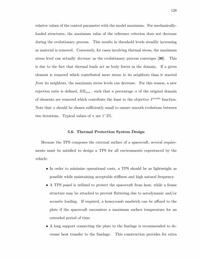
128
relative values of the control parameter with the model maximum. For mechanically-
loaded structures, the maximum value of the reference criterion does not decrease
during the evolutionary process. This results in threshold levels steadily increasing
as material is removed. Conversely, for cases involving thermal stress, the maximum
stress level can actually decrease as the evolutionary process converges [30]. This
is due to the fact that thermal loads act as body forces in the domain. If a given
element is removed which contributed more stress to its neighbors than it reacted
from its neighbors, the maximum stress levels can decrease. For this reason, a new
rejection ratio is de�ned, RRnew , such that a percentage � of the original domain
of elements are removed which contribute the least to the objective Fmulti function.
Note that � should be chosen su¢ ciently small to ensure smooth evolutions between
two iterations. Typical values of � are 1~2%.
5.6. Thermal Protection System Design
Because the TPS composes the external surface of a spacecraft, several require-
ments must be satis�ed to design a TPS for all environments experienced by the
vehicle:
� In order to minimize operational costs, a TPS should be as lightweight as
possible while maintaining acceptable sti¤ness and high natural frequency.
� A TPS panel is utilized to protect the spacecraft from heat, while a frame
structure may be attached to prevent �uttering due to aerodynamic and/or
acoustic loading. If required, a honeycomb sandwich can be a¢ xed to the
plate if the spacecraft encounters a maximum surface temperature for an
extended period of time.
� A long support connecting the plate to the fuselage is recommended to de-
crease heat transfer to the fuselage. This construction provides for extra
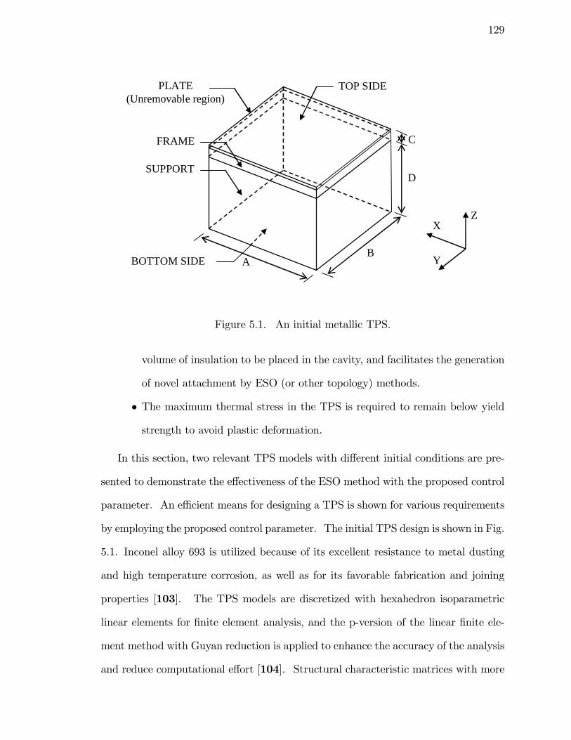
129
PLATE(Unremovable region)
C
D
BA
FRAME
SUPPORT
TOP SIDE
BOTTOM SIDE Y
XZ
Figure 5.1. An initial metallic TPS.
volume of insulation to be placed in the cavity, and facilitates the generation
of novel attachment by ESO (or other topology) methods.
� The maximum thermal stress in the TPS is required to remain below yield
strength to avoid plastic deformation.
In this section, two relevant TPS models with di¤erent initial conditions are pre-
sented to demonstrate the e¤ectiveness of the ESO method with the proposed control
parameter. An e¢ cient means for designing a TPS is shown for various requirements
by employing the proposed control parameter. The initial TPS design is shown in Fig.
5.1. Inconel alloy 693 is utilized because of its excellent resistance to metal dusting
and high temperature corrosion, as well as for its favorable fabrication and joining
properties [103]. The TPS models are discretized with hexahedron isoparametric
linear elements for �nite element analysis, and the p-version of the linear �nite ele-
ment method with Guyan reduction is applied to enhance the accuracy of the analysis
and reduce computational e¤ort [104]. Structural characteristic matrices with more
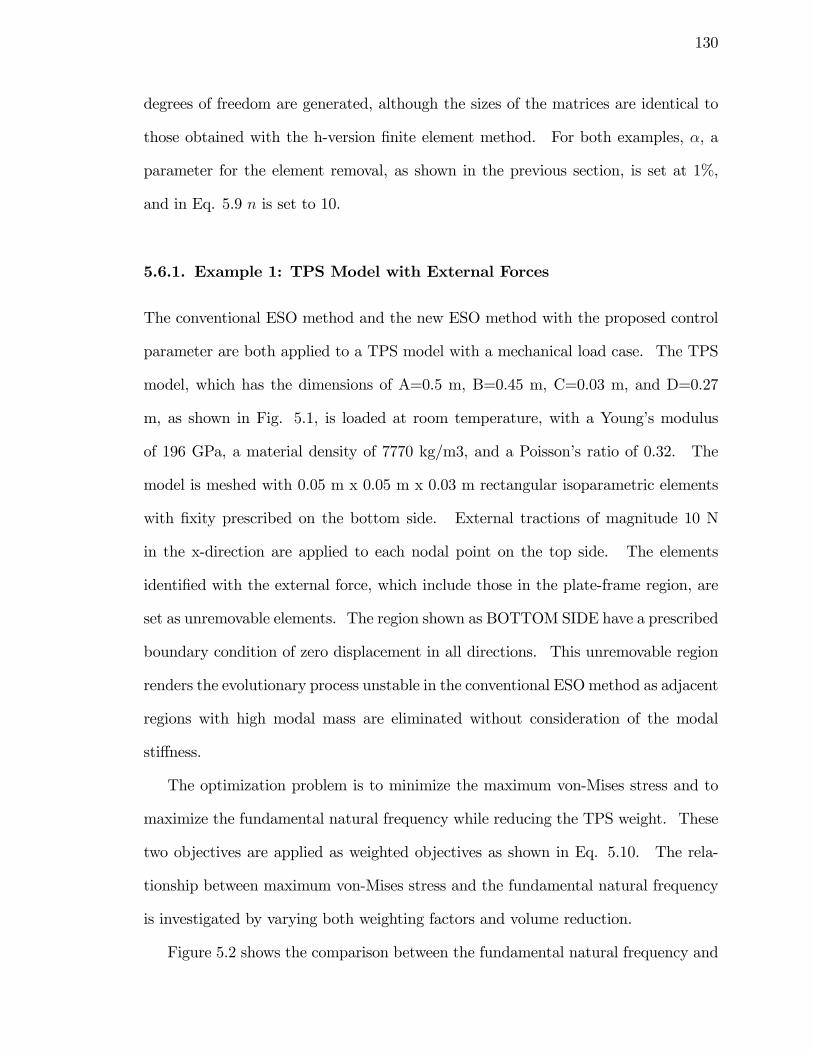
130
degrees of freedom are generated, although the sizes of the matrices are identical to
those obtained with the h-version �nite element method. For both examples, �, a
parameter for the element removal, as shown in the previous section, is set at 1%,
and in Eq. 5.9 n is set to 10.
5.6.1. Example 1: TPS Model with External Forces
The conventional ESO method and the new ESO method with the proposed control
parameter are both applied to a TPS model with a mechanical load case. The TPS
model, which has the dimensions of A=0.5 m, B=0.45 m, C=0.03 m, and D=0.27
m, as shown in Fig. 5.1, is loaded at room temperature, with a Young�s modulus
of 196 GPa, a material density of 7770 kg/m3, and a Poisson�s ratio of 0.32. The
model is meshed with 0.05 m x 0.05 m x 0.03 m rectangular isoparametric elements
with �xity prescribed on the bottom side. External tractions of magnitude 10 N
in the x-direction are applied to each nodal point on the top side. The elements
identi�ed with the external force, which include those in the plate-frame region, are
set as unremovable elements. The region shown as BOTTOM SIDE have a prescribed
boundary condition of zero displacement in all directions. This unremovable region
renders the evolutionary process unstable in the conventional ESOmethod as adjacent
regions with high modal mass are eliminated without consideration of the modal
sti¤ness.
The optimization problem is to minimize the maximum von-Mises stress and to
maximize the fundamental natural frequency while reducing the TPS weight. These
two objectives are applied as weighted objectives as shown in Eq. 5.10. The rela-
tionship between maximum von-Mises stress and the fundamental natural frequency
is investigated by varying both weighting factors and volume reduction.
Figure 5.2 shows the comparison between the fundamental natural frequency and
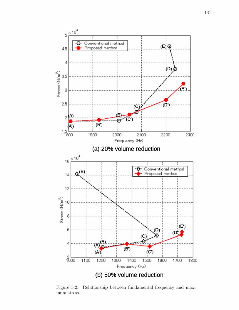
131
(a) 20% volume reduction
(b) 50% volume reduction
(a) 20% volume reduction
(b) 50% volume reduction
Figure 5.2. Relationship between fundamental frequency and maxi-mum stress.
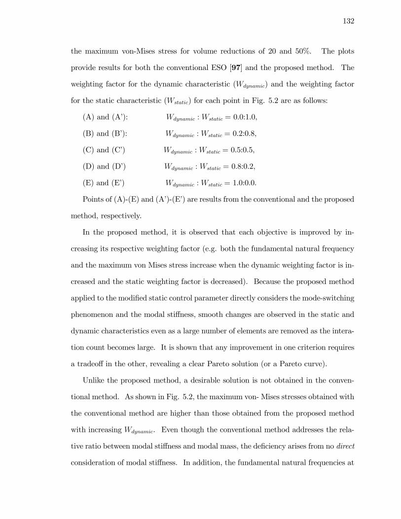
132
the maximum von-Mises stress for volume reductions of 20 and 50%. The plots
provide results for both the conventional ESO [97] and the proposed method. The
weighting factor for the dynamic characteristic (Wdynamic) and the weighting factor
for the static characteristic (Wstatic) for each point in Fig. 5.2 are as follows:
(A) and (A�): Wdynamic : Wstatic = 0.0:1.0,
(B) and (B�): Wdynamic : Wstatic = 0.2:0.8,
(C) and (C�) Wdynamic : Wstatic = 0.5:0.5,
(D) and (D�) Wdynamic : Wstatic = 0.8:0.2,
(E) and (E�) Wdynamic : Wstatic = 1.0:0.0.
Points of (A)-(E) and (A�)-(E�) are results from the conventional and the proposed
method, respectively.
In the proposed method, it is observed that each objective is improved by in-
creasing its respective weighting factor (e.g. both the fundamental natural frequency
and the maximum von Mises stress increase when the dynamic weighting factor is in-
creased and the static weighting factor is decreased). Because the proposed method
applied to the modi�ed static control parameter directly considers the mode-switching
phenomenon and the modal sti¤ness, smooth changes are observed in the static and
dynamic characteristics even as a large number of elements are removed as the intera-
tion count becomes large. It is shown that any improvement in one criterion requires
a tradeo¤ in the other, revealing a clear Pareto solution (or a Pareto curve).
Unlike the proposed method, a desirable solution is not obtained in the conven-
tional method. As shown in Fig. 5.2, the maximum von- Mises stresses obtained with
the conventional method are higher than those obtained from the proposed method
with increasing Wdynamic. Even though the conventional method addresses the rela-
tive ratio between modal sti¤ness and modal mass, the de�ciency arises from no direct
consideration of modal sti¤ness. In addition, the fundamental natural frequencies at
133
Wdynamic:Wstatic =1.0:0.0 are decreased by this lack of modal sti¤ness as well as the
changing control parameter characteristics due to mode-switching. Determining the
trend of the Pareto solution with volume reduction is extremely di¢ cult. However,
in constrast to the conventional method, the proposed control parameter can be used
to design an optimum structure as a large number of elements are eliminated through
many iterations and yet provide constructive dynamic modi�cation.
5.6.2. Example 2: TPS Model with Thermal Loading
When a spacecraft re-enters the atmosphere from Low Earth Orbit (LEO), the tremen-
dous heat �uxes generated produce a non-uniform, transient temperature distribution
in the metallic TPS. Since most metallics demonstate temperature dependence, the
thermal (thermal conductivity and speci�c heat) and mechanical (Young�s modulus
and coe¢ cient of thermal expansion) properties will vary with temperature in the
TPS. This temperature dependence in the thermal problem results in nonlinearity
and necessitates an iterative solution technique.
For the second example, a transient thermal pro�le is applied to the initial TPS
model in Fig. 5.1. The (void) space inside the TPS and the vertical surface bound-
aries (with the exception of the surface of the plate) are treated as insulated. The
plate temperature (Tplate) on the top side varies according to a temperature pro-
�le, as shown in [105]. In this method, the temperature is simply represented as
Tplate = 1:2540t+200 C when (t < 500 sec:), and Tplate = 827 C when (t � 500 sec:),
regardless of the elimination of elements from the structure. This assumption is a
severe restriction. In the true structure, convection and radiation play major roles
in the transfer of energy. For instance, to address the internal radiative heat trans-
fer that will occur as material is removed, an e¢ cient method for constructing view
factors during the iterative process would be needed. Since the purpose of this work
134
was to develop an ESO method for simultaneous consideration of thermal stress and
frequency, prescribed temperature boundary conditions were used to ensure tractabil-
ity.
A numerical time integration scheme,[106] similar to Newmark�s method, is used
to solve the following transient heat transfer problem
(5.11) (1
�t[Mt]+�[Kt])fTi+1g = [
1
�t[Mt]� (1��)[Kt]]fTig+(1��)fFig+�fFi+1g
where [Mt] is the consistent mass matrix; [Kt] is the thermal conductivity matrix; fFig
is the thermal force vector created from heat sources (or heat sinks), heat �uxes, and
convective boundary conditions; �t is the time step; � is an integration parameter
set to 0.5 (Crank-Nicolson rule); and fTig & fTi+1gare the nodal temperatures at
time ti and ti+1, respectively. To reduce the computational time of the transient
analysis, only the tendency of the temperature pro�le at t = 1500 sec is evaluated
by assuming that [Mt] and [Kt] are constant with time as thermal conductivities
(Kxx = Kyy = Kzz = 20 W/(m-C)), density ( �=7770 kg/m3), and speci�c heat
(c =530 J/(kg-C)) are treated as temperature-independent variables. A constant
timestep of �t =10 sec. is considered. The initial temperature distribution fTog for
each iterative process is assumed to be a linear pro�le through the thickness with 127
C on the top side and 27 C on the bottom side.
5.6.2.1. Applicability of the Proposed Control Parameter to a Transient
Thermal Pro�le. Both conventional and proposed methods are compared to demon-
strate the applicability of the proposed control parameter for topology optimization
of a TPS with a non-uniform temperature pro�le. The TPS model has dimensions
A=0.48 m, B=0.42 m, C=0.03m, and D is intentionally set 0.27 m longer than typical
TPS structures [107] to reduce thermal stress in the �xed regions at the bottom side
(interface to low-temperature material). The plate and frame regions are treated as
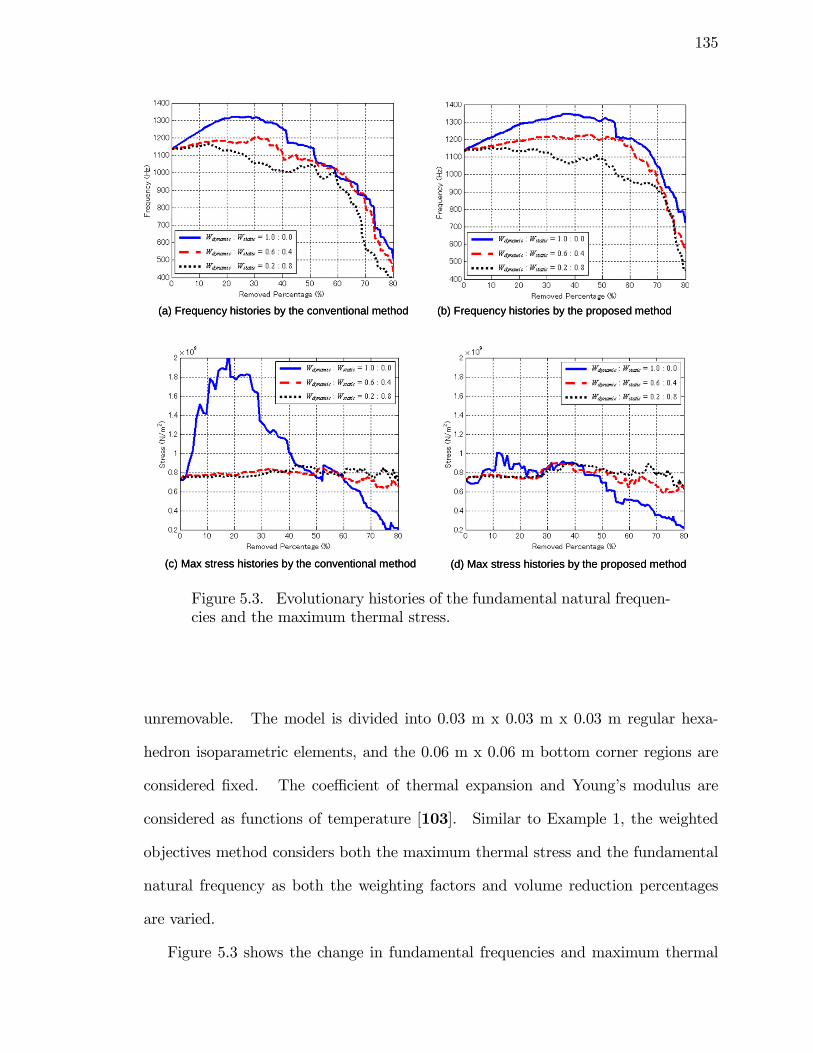
135
(a) Frequency histories by the conventional method (b) Frequency histories by the proposed method
(c) Max stress histories by the conventional method (d) Max stress histories by the proposed method
(a) Frequency histories by the conventional method (b) Frequency histories by the proposed method
(c) Max stress histories by the conventional method (d) Max stress histories by the proposed method
Figure 5.3. Evolutionary histories of the fundamental natural frequen-cies and the maximum thermal stress.
unremovable. The model is divided into 0.03 m x 0.03 m x 0.03 m regular hexa-
hedron isoparametric elements, and the 0.06 m x 0.06 m bottom corner regions are
considered �xed. The coe¢ cient of thermal expansion and Young�s modulus are
considered as functions of temperature [103]. Similar to Example 1, the weighted
objectives method considers both the maximum thermal stress and the fundamental
natural frequency as both the weighting factors and volume reduction percentages
are varied.
Figure 5.3 shows the change in fundamental frequencies and maximum thermal
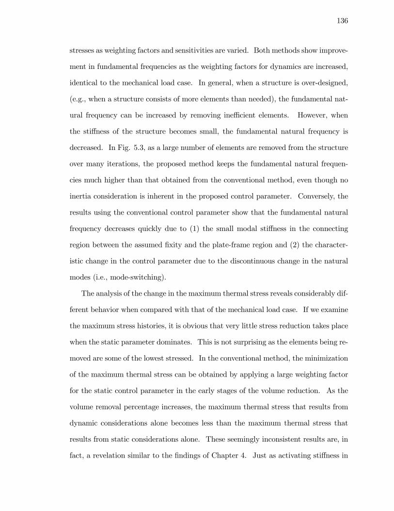
136
stresses as weighting factors and sensitivities are varied. Both methods show improve-
ment in fundamental frequencies as the weighting factors for dynamics are increased,
identical to the mechanical load case. In general, when a structure is over-designed,
(e.g., when a structure consists of more elements than needed), the fundamental nat-
ural frequency can be increased by removing ine¢ cient elements. However, when
the sti¤ness of the structure becomes small, the fundamental natural frequency is
decreased. In Fig. 5.3, as a large number of elements are removed from the structure
over many iterations, the proposed method keeps the fundamental natural frequen-
cies much higher than that obtained from the conventional method, even though no
inertia consideration is inherent in the proposed control parameter. Conversely, the
results using the conventional control parameter show that the fundamental natural
frequency decreases quickly due to (1) the small modal sti¤ness in the connecting
region between the assumed �xity and the plate-frame region and (2) the character-
istic change in the control parameter due to the discontinuous change in the natural
modes (i.e., mode-switching).
The analysis of the change in the maximum thermal stress reveals considerably dif-
ferent behavior when compared with that of the mechanical load case. If we examine
the maximum stress histories, it is obvious that very little stress reduction takes place
when the static parameter dominates. This is not surprising as the elements being re-
moved are some of the lowest stressed. In the conventional method, the minimization
of the maximum thermal stress can be obtained by applying a large weighting factor
for the static control parameter in the early stages of the volume reduction. As the
volume removal percentage increases, the maximum thermal stress that results from
dynamic considerations alone becomes less than the maximum thermal stress that
results from static considerations alone. These seemingly inconsistent results are, in
fact, a revelation similar to the �ndings of Chapter 4. Just as activating sti¤ness in
137
a direction orthogonal to the in-plane direction to minimize in-plane load, was shown
to be a successful approach to minimize boundary loads (Chapter 4), when the modal
sti¤ness is biased toward the out-of-plane direction (i.e., bending of the top plate),
stress reduction occurs. The von-Mises stress measure does not distinguish between
tension or compression. When the optimizer is removing material for all modes ex-
cept the out-of-plane direction, the other frequencies are being reduced. Granted
they are still higher than the mode of interest, but they will approach the bending
mode in the limit. The modal sti¤ness in these other orthgonal modes correspond
to static sti¤ness as well. Hence, this e¤ect renders the structure less equipped to
support high compression loads (or reaction forces) for the in-plane directions. As
the volume reduction proceeds, to maintain high frequency, the material is focused
on suppressing bending in the un-removeable plate region. By focusing material in
such a manner, the sti¤ness is focused directly into the out-of-plane bending mode at
the expense of the other modes. Since no mechanical boundary condition constrains
the thermal expansion of the TPS in the Z-direction, thermal stress is relieved as
frequency remains high even for large values of volume reduction.
Figure 5.4 shows resulting models close to 900 Hz in fundamental natural fre-
quency by both the conventional and proposed methods. Each model is developed
using solely dynamic considerations, that is, Wdynamic : Wstatic = 1:0 : 0:0. The
fundamental natural frequency, maximum stress, and the number of elements result
in 933.6 Hz, 0.523 GPa, and 740 (155.2 kg) using the conventional method, and 906.8
Hz, 0.330 GPa, and 568 (119.2 kg) by the proposed method. The main di¤erence
between the two resulting topologies is the location of the elements that are adjacent
to the plate-frame region: one is located towards the center of the plate-frame region,
and the other is located towards the edges of the plate-frame region. The conclusion
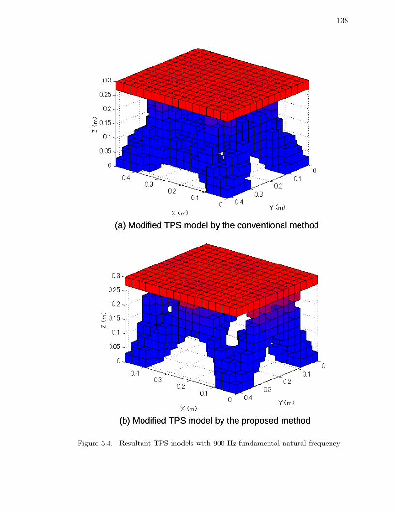
138
(a) Modified TPS model by the conventional method
(b) Modified TPS model by the proposed method
(a) Modified TPS model by the conventional method
(b) Modified TPS model by the proposed method
Figure 5.4. Resultant TPS models with 900 Hz fundamental natural frequency
139
to be drawn from this study is the proposed method is superior to the conventional
method in both maintaining high fundamental frequency and reducing thermal stress.
From the above results, the ESO method with the proposed control parameter
can be used to design a lightweight TPS model with a high fundamental natural
frequency and a low maximum thermal stress. Using the assumption that only
conduction a¤ects the support region, a practical TPS design is developed by using
Wdynamic : Wstatic = 1:0 : 0:0 in the next section.
5.6.2.2. Detailed TPS Design with Thermal Transient Pro�le. In contrast
to the static case, the convergence of the eigenvalue maximization problem presents
a more daunting task. In an evolutionary procedure that requires a large number
of element removals over many iterations, the ordering of natural modes may be
altered by selection of the initial geometry. Considering the initial geometry as an
input, considerable variations in structural characteristics (i.e. neighboring natural
frequencies, weight of the structure, etc.) can result. Therefore, appealing to the
topology results of the previous section (Fig. 5.4 (b)), the initial TPS model is
chosen to be that of Fig. 5.4 (b) with a slight modi�cation. Element removal is only
permitted on the inside of the structure, as shown in Fig. 5.5. A shape optimization
method based on the ESO technique (called �nibbling ESO [54]) is applied to the
support region to avoid the checkerboard pattern that occurred in Fig. 5.4 (b). That
is, only the structural boundaries in the Z direction between Layer 1 and Layer 10
(with the exception of the unremovable Layer 0 region ) are removed from the model.
The frame region, as well as the support region, are designed to reduce the TPS
weight. Using the proposed method, the objectives take the following form:
Minimize TPS weight
subject to
(1) maximization of the fundamental natural frequency (f1 � 900 Hz)
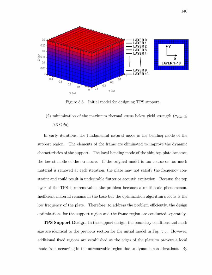
140
Figure 5.5. Initial model for designing TPS support
(2) minimization of the maximum thermal stress below yield strength (�max �
0:3 GPa)
In early iterations, the fundamental natural mode is the bending mode of the
support region. The elements of the frame are eliminated to improve the dynamic
characteristics of the support. The local bending mode of the thin top plate becomes
the lowest mode of the structure. If the original model is too coarse or too much
material is removed at each iteration, the plate may not satisfy the frequency con-
straint and could result in undesirable �utter or acoustic excitation. Because the top
layer of the TPS is unremovable, the problem becomes a multi-scale phenomenon.
Ine¢ cient material remains in the base but the optimization algorithm�s focus is the
low frequency of the plate. Therefore, to address the problem e¢ ciently, the design
optimizations for the support region and the frame region are conducted separately.
TPS Support Design. In the support design, the boundary condtions and mesh
size are identical to the previous section for the initial model in Fig. 5.5. However,
additional �xed regions are established at the edges of the plate to prevent a local
mode from occurring in the unremovable region due to dynamic considerations. By
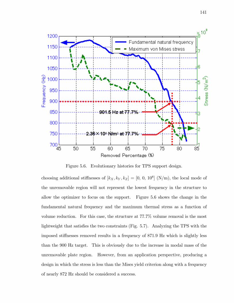
141
Figure 5.6. Evolutionary histories for TPS support design.
choosing additional sti¤nesses of [kX ; kY ; kZ ] = [0, 0, 108] (N/m), the local mode of
the unremovable region will not represent the lowest frequency in the structure to
allow the optimizer to focus on the support. Figure 5.6 shows the change in the
fundamental natural frequency and the maximum thermal stress as a function of
volume reduction. For this case, the structure at 77.7% volume removal is the most
lightweight that satis�es the two constraints (Fig. 5.7). Analyzing the TPS with the
imposed sti¤nesses removed results in a frequency of 871.9 Hz which is slightly less
than the 900 Hz target. This is obviously due to the increase in modal mass of the
unremovable plate region. However, from an application perspective, producing a
design in which the stress is less than the Mises yield criterion along with a frequency
of nearly 872 Hz should be considered a success.
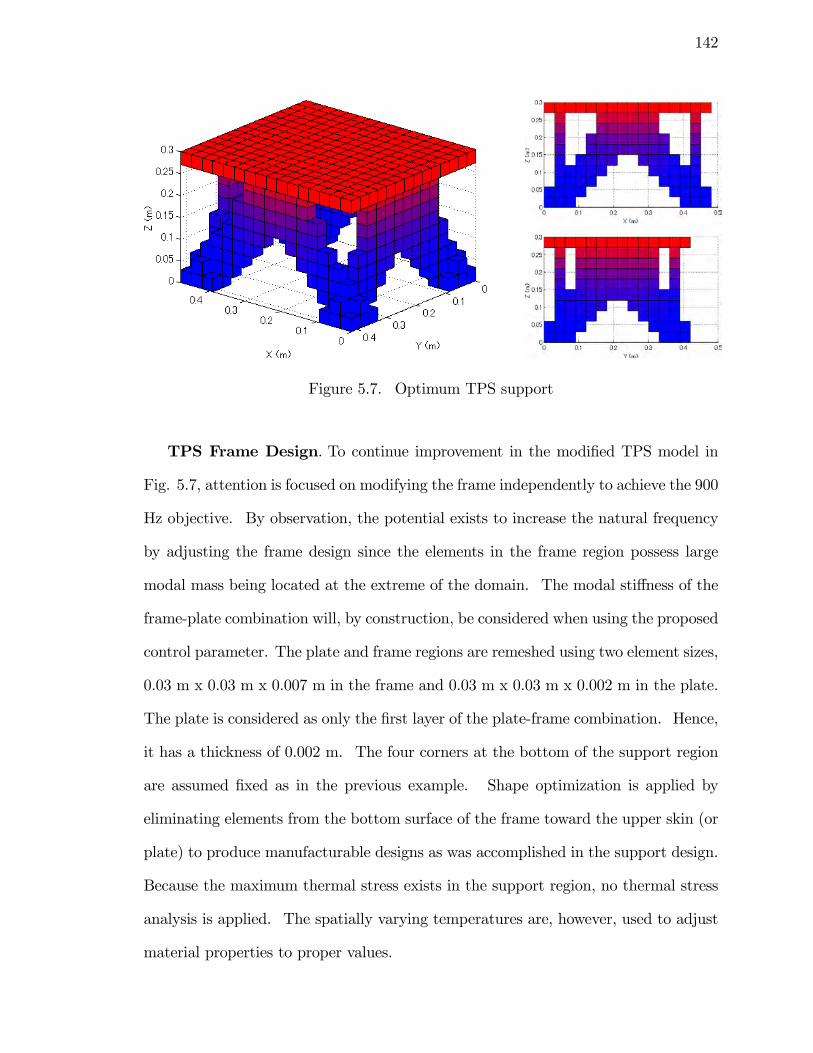
142
Figure 5.7. Optimum TPS support
TPS Frame Design. To continue improvement in the modi�ed TPS model in
Fig. 5.7, attention is focused on modifying the frame independently to achieve the 900
Hz objective. By observation, the potential exists to increase the natural frequency
by adjusting the frame design since the elements in the frame region possess large
modal mass being located at the extreme of the domain. The modal sti¤ness of the
frame-plate combination will, by construction, be considered when using the proposed
control parameter. The plate and frame regions are remeshed using two element sizes,
0.03 m x 0.03 m x 0.007 m in the frame and 0.03 m x 0.03 m x 0.002 m in the plate.
The plate is considered as only the �rst layer of the plate-frame combination. Hence,
it has a thickness of 0.002 m. The four corners at the bottom of the support region
are assumed �xed as in the previous example. Shape optimization is applied by
eliminating elements from the bottom surface of the frame toward the upper skin (or
plate) to produce manufacturable designs as was accomplished in the support design.
Because the maximum thermal stress exists in the support region, no thermal stress
analysis is applied. The spatially varying temperatures are, however, used to adjust
material properties to proper values.
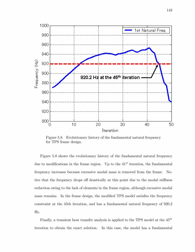
143
Figure 5.8. Evolutionary history of the fundamental natural frequencyfor TPS frame design.
Figure 5.8 shows the evolutionary history of the fundamental natural frequency
due to modi�cations in the frame region. Up to the 41st iteration, the fundamental
frequency increases because excessive modal mass is removed from the frame. No-
tice that the frequency drops o¤ drastically at this point due to the modal sti¤ness
reduction owing to the lack of elements in the frame region, although excessive modal
mass remains. In the frame design, the modi�ed TPS model satis�es the frequency
constraint at the 45th iteration, and has a fundamental natural frequency of 920.2
Hz.
Finally, a transient heat transfer analysis is applied to the TPS model at the 45th
iteration to obtain the exact solution. In this case, the model has a fundamental
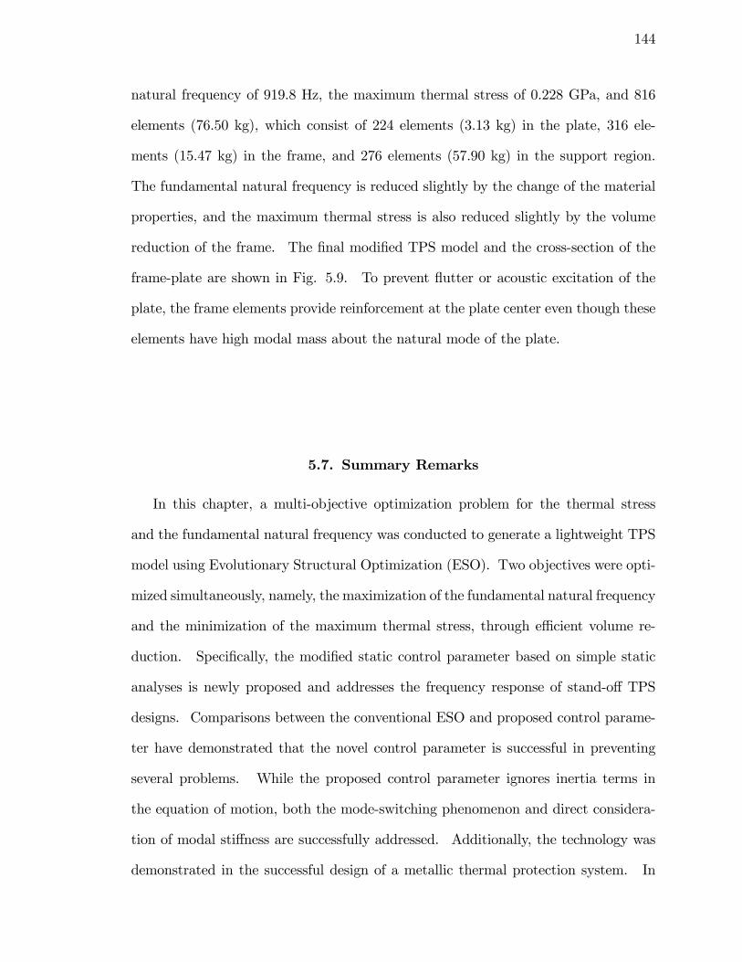
144
natural frequency of 919.8 Hz, the maximum thermal stress of 0.228 GPa, and 816
elements (76.50 kg), which consist of 224 elements (3.13 kg) in the plate, 316 ele-
ments (15.47 kg) in the frame, and 276 elements (57.90 kg) in the support region.
The fundamental natural frequency is reduced slightly by the change of the material
properties, and the maximum thermal stress is also reduced slightly by the volume
reduction of the frame. The �nal modi�ed TPS model and the cross-section of the
frame-plate are shown in Fig. 5.9. To prevent �utter or acoustic excitation of the
plate, the frame elements provide reinforcement at the plate center even though these
elements have high modal mass about the natural mode of the plate.
5.7. Summary Remarks
In this chapter, a multi-objective optimization problem for the thermal stress
and the fundamental natural frequency was conducted to generate a lightweight TPS
model using Evolutionary Structural Optimization (ESO). Two objectives were opti-
mized simultaneously, namely, the maximization of the fundamental natural frequency
and the minimization of the maximum thermal stress, through e¢ cient volume re-
duction. Speci�cally, the modi�ed static control parameter based on simple static
analyses is newly proposed and addresses the frequency response of stand-o¤ TPS
designs. Comparisons between the conventional ESO and proposed control parame-
ter have demonstrated that the novel control parameter is successful in preventing
several problems. While the proposed control parameter ignores inertia terms in
the equation of motion, both the mode-switching phenomenon and direct considera-
tion of modal sti¤ness are successfully addressed. Additionally, the technology was
demonstrated in the successful design of a metallic thermal protection system. In
145
(a) Optimum TPS model
(i) Z = 0.270 m (ii) Z = 0.277 m (iii) Z = 0.284 m
(iv) Z = 0.291 m (v) Z = 0.298 m (vi) Z = 0.3 m (Plate)
(b) Crosssection in the plateframe region
(a) Optimum TPS model
(i) Z = 0.270 m (ii) Z = 0.277 m (iii) Z = 0.284 m
(iv) Z = 0.291 m (v) Z = 0.298 m (vi) Z = 0.3 m (Plate)
(b) Crosssection in the plateframe region
Figure 5.9. Optimum TPS model including heat transfer e¤ects.
future work, consideration will be given to more realistic thermal conditions. Inclu-
sion of convection and radiation as well as a maximum temperature constraint could
potentially result in new and innovative designs.
CHAPTER 6
Summary and Future Work
6.1. Summary
In this work, the design of thermal structures using topology optimization is ex-
plored. The primary motivation for this work rests in the design of low-observable,
engine exhaust-washed structures. Embedded engines require a surface on which
to expel exhaust gases. This protective covering must survive the thermal stresses
while performing its function of shielding the lower temperature substructure from
the extreme thermal environment. Of particular concern is the out-of-plane defor-
mation of the thin covering. Conventional sti¤ening methods are demonstrated to
be problematic as tremendous additional loads into sub and surrounding structure
can occur. The non-intuitive nature of sti¤ening thin panels (both �at and curved)
in a thermal environment are explored in detail. The �ndings reveal that adding to
the thickness of a panel will not only increase load into surrounding structure, but
can also increase the maximum tensile stress in the panel.
The Simple Isotropic Material with Penalization (or SIMP) minimum compli-
ance topology optimization is applied to the thermally-loaded problem and found be
highly non-optimal as material is distributed close to the original thickness of the
panel. However, a minimum compliance formulation is presented which applies me-
chanical loads in such a way as to activate sti¤ness only in the out-of-plane direction.
This formulation renders the design incapable of producing large loads in the in-plane
146

147
direction when heated. The bridge-type sti¤ening structures generated share a com-
mon characteristic in that internal thermal expansion can occur, limiting the reaction
load.
A novel ESO control parameter is developed to address both sti¤ness and fre-
quency simultaneously. Mises stress and fundamental frequency are combined in a
weighted objective formulation while volume is reduced to achieve acceptability in
both responses. Similar to the exhaust-washed structure, a generic, metallic thermal
protection system is designed. A non-uniform temperature pro�le is applied to the
structure and a successful evolutionary design is achieved with von-Mises stress less
than yield and �rst fundamental frequency above 900 Hz. The novel control para-
meter addresses two major concerns in frequency optimization. The �rst remedies
the three-dimensional e¤ect where the mode of interest exchanges with a di¤erent
mode which is much lower after structural modi�cation. The second pathology that
is mitigated is the inadequacy of previous ESO frequency optimization schemes to
directly address modal sti¤ness. The newly-derived control parameter achieves this
end. The ESO method applied to TPS design demonstrates the same characteris-
tics as the SIMP formulation in that lower stress (or lower reaction force) designs are
achieved when only frequency optimization is the goal and that frequency corresponds
to an out-of-plane mode.
6.2. Adjoint Topology Formulation for Direct Consideration of
Load-Stress Trade Space
While the two topology optimization formulations given above produce reason-
able designs and extend the knowledge base of thermoelastic topology optimization,
a more direct approach to reducing stress and limiting reaction load is needed. The
148
procedure presented in Chapter 4 does limit the load into the boundary by construc-
tion, but further methods (shape and sizing optimization) are required to satisfy a
stress objective. The ESO method presented in Chapter 5 limits the von-Mises stress
(and hence the reaction load) to some degree but no direct prescription is made. In
this section, a methodology will be presented which directly exposes the stress-load
trade space and no restriction is made regarding the linearity of the analysis.
This development follows closely to that presented in [108] with the inclusion of
the thermal expansion e¤ects. The nonlinear thermo-elastic boundary value problem
is initially posed in the strong form. A reformulation of the problem statement into
the weak form provides a convenient transistion to the �nite element discretization.
A residual equation is presented which is solved by the Newton-Raphson nonlinear
simultaneous equation solver. And �nally, an implementation scheme for incorpo-
rating this capability into the commerical code ABAQUS via a user-de�ned element
(UEL) is discussed.
6.2.1. Thermoelastic Boundary Value Problem
Using the construct for a Lagrangian, material-based formulation as found in [34], a
material point � is located by the position vectorX in the undeformed con�guration
o of the body. Kinematically, the body experiences a displacement �eld u (X)
which results in the mapping f : X �! x where x is the position vector in the
current con�guration of the body. The total strain E is de�ned through the
deformation gradient F ,
(6.1) F (X) = I +ru (X)
149
(6.2) E (X) =1
2
�ru (X) +ruT (X) +ruT (X)ru (X)
�Since thermal expansion e¤ects will be included, we must di¤erentiate between
the total strain and the mechanical strain Emech as the mechanical strain is the
appropriate strain measure for constitutive equation. The total strain is comprised
of both Emech (Eq. 6.3) and the thermal strain Eth
(6.3) Emech = E �Eth
with the thermal strain given by Eq. 6.4
(6.4) Eth (X) = �4T (X)I
The coe¢ cient of thermal expansion, �, can in general be a function of the spatially-
varying temperature di¤erence, 4T (X). The temperature di¤erence �eld, 4T (X) ;
is measured relative to a reference temperature, 4T (X) = T (X)� Tref .
If we assume that inertial e¤ects are negligible (which may not be the case if
thermal transients are large), the system response is treated as quasi-static; therefore,
the strong forms of local linear and angular momentum balance are respectively given
by
div (F (X)T o(X)) + b0(X) = 0(6.5)
T o(X) = T To (X)(6.6)
where T o(X) is the symmetric 2nd Piola-Kirchho¤ stress tensor and b0(X) is the
body force vector de�ned per unit original (undeformed) volume.
150
A hyperelastic material response is assumed which implies path independence
of the material response. The hyperelastic assumption also guarantees that the
stress response can be derived from a strain energy e(X) =�e(Emech (X) ;X) de�ned
on the undeformed con�guration. The 2nd Piola-Kirchho¤ stress tensor T o(X) is
the derivative of the strain energy�e with respect to the mechanical strain tensor
Emech (X) ;i.e.T o(X) = @�e
@Emech: In this work, the materials considered are high tem-
perature, isotropic metallic alloys, and it follows that small strains may be assumed
while the structure may undergo large displacements. The hyperelastic material
model introduced is adequate to describe the material behavior, i.e.
�e =
�E
2 (1 + �)(1� 2�)tr(Emech)2 +
E
2(1 + �)tr(E2
mech)(6.7)
T o =@�e
@Emech
= CEmech(6.8)
where the elasticity tensor C depends on two material parameters, Young�s modulus
E and Poisson�s ratio �. These material constants should be familiar to the reader
as they de�ne the familiar Hooke�s law for a linear isotropic material. Experimental
results have shown Young�s modulus to be a decreasing function of temperature for
most engineering materials. Therefore, if the range of operating temperatures is
signi�cant, E should include the temperature dependence.
A boundary value problem de�nition is incomplete without speci�cation of bound-
ary conditions. Displacement and surface traction boundary conditions are pre-
scribed as uP and tP on the complementary boundariesAu0 andA
t0 of the undeformed
con�guration. The essential and natural boundary conditions are given by
u(X) = up(X) X � Au0(6.9)
F (X)T 0(X)n0(X) = tp(X) X � At0(6.10)
151
The solution to the boundary value problem is known once the displacement �eld is
determined.
6.2.2. Weak Formulation
The thermoelastic boundary value problem is recast into an equivalent variational (or
weak) form. The familiar weak form is generated by multiplying both the equilib-
rium Eq. 6.5 and the natural (traction) boundary condition (Eq. 6.10) by a weight
function v and integrating over the appropriate domains. Satisfaction of the essen-
tial boundary conditions is ensured by restricting u and v to the set of kinematically
admissible displacements. Conservation of angular momentum (Eq. 6.6) is ensured
by the proper choice of material constitutive law. After integration by parts and an
application of the divergence theorem, a residual equation is formed by the equivalent
weak form.
(6.11) g(u) = 0 = �Z0
rv � (FT 0) dv0 +Z0
v � b0dv0 +ZAt0
v � tpda0
The constitutive equation (Eq. 6.8), the strain-displacement relation (Eq. 6.2), and
the mechanical strain (Eq. 6.3) are substituted into Eq. 6.11.
g(u) = 0 = �Z0
rv � (FC (E � Eth)) dv0 +
Z0
v � b0dv0 +ZAt0
v � tpda0(6.12)
= 0 = �Z0
rv � (F (CE))dv0 +Z0
rv � (F (CEth)) dv0 +Z0
v � b0dv0 +ZAt0
v � tpda0
One important observation should be noted in Eq. 6.12 is the resemblence of the
thermal stress work to a body force. In fact, the thermal-elasic equations are identical
to the elastic relations with the work of the thermal stress included as a volume
152
integral over the reference volume. The solution of the responses are found by
discretizing the domain and applying the Galerkin �nite element method.
The system version of the Newton-Raphson nonlinear equation solver is used to
solve the nonlinear algebraic �nite element equations. The Newton-Raphson solver
is characterized by second-order convergence and the formation of a tangent matrix
which is used in subsequent design sensitivity analysis. The nonlinlear �nite element
equation G, expressed as a function of the nodal response vector U , is given in
residual form by
(6.13) G(U) = 0
The development of the Newton-Raphson method follows from a �rst-order Taylor
series expansion of Eq. 6.13. The expansion is performed about the current solution
U i
(6.14) G(U i+1) � G(U i )+DG
DU(U i) �U = 0
where �U = U i+1�U i represents the update to the response vector. Rearrangement
of Eq. 6.14 gives the familiar �nite element form
(6.15) KT (U i) �U = G(U i)
where KT (U i) � �DGDU
(U i) is the tangent (sti¤ness) matrix. Iterative is continued
until either (or both) the magnitudes of the residual and response update is less than
a speci�ed value.
153
6.2.3. Finite Element Formulation
For solution expediency, the residual �nite element equations are decomposed into
internal and external force vectors,
(6.16) G(U) = 0 = S(U) + F
where
(6.17) S = �Z0
rv � (FT 0) dv0
is the virtual work of the internal force vector and
(6.18) F =
Z0
rv � (F (CEth)) dv0 +
Z0
v � b0dv0 +ZAt0
v � tpda0
is the virtual work done by the external forces. The displacement vector is partitioned
into an unknown free displacement vector U f and a known prescribed displacement
vector U p. In explicit vector form,
(6.19) U =
8><>:Uf
U p
9>=>;Since only the free degrees of freedom will be solved, it is convenient to partition the
residual equation into Gf and Gp vectors as
(6.20) G�U p;U f
�=
8><>:Gf�U p;U f
�Gp�U p;U f
�9>=>; =
8><>:Sf�U p;U f
�Sp�U p;U f
�9>=>;+
8><>:PR9>=>; = 0
where P and R are the applied and reaction force vectors, respectively. In this de-
velopment, P will be independent of the displacement response, however, the thermal
loading will depend on the design.
154
The nonlinear equation Gf is solved for the unknown free displacement vector
U f using the Newton-Raphson method. The tangent sti¤ness matrix in terms of the
solution variables is given by
(6.21) KT = �@Gf
@U f
�U p;U f
�In �nite element parlance, the computation or recovery of the unknown reaction forces
can be accomplished by appealing to the second residual in Eq. 6.20 after the solution
of Uf is obtained.
6.2.4. Topology Optimization
The topology optimization problem is stated as
min �o(d)(6.22)
subject to �i(d) � 0
d¯ j� dj � �dj
where �o is the objective function, �i (i = 1; : : :) are the inequality or equality
constraints and dj (j = 1; : : :) are the design variables that are bounded above and
below by d¯ jand �dj. The design variable in this scenario is taken as a density variable
de�ned over each element. To ensure a mesh independent design, a �lter should be
employed.
6.2.5. Adjoint Sensitivity Analysis
As discussed previously in Chapters 3 and 4, the design variables typically consist
of a density measure de�ned over each element. The most common implementation
employs a single element density variable over each element. Therefore, the number
155
of design variables equals the number of elements. Since the problem under con-
sideration is nonlinear, many iterations will be required for solution and subsequent
convergence. Hence a premium is placed on e¢ cient sensitivity computation.
For systems with large numbers of design variables but few objective and con-
straint equations are most e¢ ciently solved by applying the adjoint sensitivity method
[43] The adjoint formulation for the topology problem is constructed by augmenting
the objective function with the constraint equations via Lagrange multipliers (Eq.
6.23).
�̂k(d)= � k(UP (d);Uf (d);R(d);d) + �f �Gf (UP (d);Uf (d);d)+(6.23)
�f � (SP (UP (d);Uf (d);d) +R(d))
The sensitivities are computed by di¤erentiating Eq. 6.23 with respect to the design
variables d. The result is manipulated such that the coe¢ cients of the response
sensititivies are equated to zero. The enforcement of this side condition results in
the adjoint problem. The Lagrange multipliers are obtained by solving the adjoint
problem for each objective and constraint equation. This process can be very e¢ cient
if the decomposed tangent sti¤ness matrix is available. Assuming this case, the
adjoint solution is obtained by a simple back substitution.
For the case of a clamped, curved panel subjected to thermal loading, the objective
consists of matching the deformed displacement �eld to a prescribed �eld with a more
benign tensile stress response. A single constraint that captures the increase in force
at the clamped boundary would provide the correct trade space.
156
6.2.6. ABAQUS Implementation
To implement this formulation in the commercial package ABAQUS, a user-de�ned
element (UEL) would be necessary. The user would be required to implement the
necessary shape functions and solution residuals desired by the ABAQUS solver. This
step is necessary because the sensitivity arrays would need to be de�ned in the UEL
so that at the end of the analysis, the adjoint problem could be solved by treating
them as additional load cases. By using the load case feature in ABAQUS, the
nonlinear problem would not require multiple solutions. While the tangent sti¤ness
is not directly available to the user, the implementation outlined would possess the
desired e¢ ciency.
References
[1] Earl A. Thornton, editor. Aerospace Thermal Structures and Materials for aNew Era. American Institute of Aeronatics and Astronautics, Inc., 1995.
[2] Shae¤er, Tuley, and Knott. Radar Cross Section. SciTech Publishing, 2004.
[3] J. Goodman, R.V. Kohn, and L. Reyna. Numerical study of a relaxed variationalproblem from optimal design. Computer Methods in Applied Mechanics andEngineering, (57):107�127, 1986.
[4] Thomas Borrvall and Joakim Petersson. Topology optimization of �uids instokes �ow. International Journal for Numerical Methods in Fluids, 41(1):77�107, 2002.
[5] O. Sigmund. Topology optimization in multiphysics problems. InAIAA/USAF/NASA/ISSMO Symposium on Multidisciplinary Analysisand Optimization, St. Louis, MO, September 1998.
[6] B.A. Boley and J.H. Weiner. Theory of Thermal Stresses. John Wiley and Sons,Inc., 1960.
[7] B.E. Gatewood. Thermal Stresses. McGraw-Hill Book Company, Inc., 1957.
[8] R.P. Hallion. Supersonic Flight, The Story of the Bell X-1 and Douglas D-558.Macmillan, New York, 1972.
[9] Jay Miller. The X-Planes, X-1 to X-29. Specialty Press, Marine on St. Croix,MN, 1983.
[10] N.J. Ho¤. High temperature e¤ects in aircraft structures. Applied MechanicsReviews, 8(11):453�456, 1955.
[11] W.H. Stillwell. X-15 research results with selected bibliography. NASA SP-60,1955.
[12] Earl A. Thornton. Thermal buckling of plates and shells. Applied MechanicsReviews, 46(10):485�506, October 1993.
[13] S. Timoshenko and J.S. Gere. Theory of Elastic Stability. McGraw-Hill, 1961.
157
158
[14] Jon Lee. Displacment and strain statistics of thermally buckled plates. InAIAA/ASME/ASCE/AHS/ASC Structures, Structural Dynamics, and Mate-rials Conference, volume 3, St. Louis, MO, April 1999.
[15] M.L. Gossard, P. Seide, and W.M. Roberts. Thermal Buckling of Plates. NACATN 2771, 1952.
[16] MWWilcox and LE Clemmer. Large de�ection analysis of heated plates. Jour-nal of the Engineering Mechanics Division, Proc ASCE, 20:165�189, 1964.
[17] Theodore Tauchert. Thermally induced �exure, buckling and vibration of plates.Applied Mechanics Reviews, 44(8):347�360, August 1991.
[18] P.M. Naghdi. On the theory of thin elastic shells. Quarterly of Applied Mathe-matics, 14:369�380, 1957.
[19] J.L. Ericksen and C. Truesdell. Exact theory of stress and strain in rods andshells. Archive for Rational Mechanics and Analysis, 1:295�323, 1958.
[20] J.L. Sanders. Nonlinear theories for thin shells. Quarterly of Applied Mathemat-ics, 21:21�36, 1963.
[21] H. Kraus. Thin Elastic Shells. Wiley, 1967.
[22] D.O. Brush and B.O. Almroth. Buckling of Bars, Plates, and Shells. McGraw-Hill, New York, 1975.
[23] Henry L. Langhaar. Energy Methods in Applied Mechanics. Robert E. KriegerPublishing Company, Malabar, FL, 1989.
[24] N.J. Ho¤. Thermal buckling of supersonic wing panels. Journal of AeronauticalSciences, 23:1019�1028, 1956.
[25] N.J. Ho¤. Buckling of a thin-walled circular cylindrical shell heated along anaxial strip. Journal of Applied Mechanics, 31:253�258, 1964.
[26] N.J. Ho¤. A nonlinear model study of the thermal buckling of thin elastic shells.Journal of Applied Mechanics, 32:71�75, 1965.
[27] M.A. Mahayni. Thermal buckling of shallow shells. International Journal ofSolids and Structures, 2:167�180, 1966.
[28] J. Wolf and W.F. Brown. Aerospace structual metals handbook. Technical Re-port AFML-TR-68-115, Air Force Materials Lab, 1974.
[29] O.C. Zienkiewicz and R.L. Taylor. The Finite Element Method, Vol 1: BasicFormulation and Linear Problems. McGraw-Hill Book Company (UK) Limited,London, 1989.
159
[30] Li Shirong and Cheng Changjun. Analysis of thermal post-buckling of heatedelastic rods. Applied Mathematics and Mechanics, 21:133�140, 2000.
[31] Li Shirong, You-He Zhou, and Xiaojing Zheng. Thermal post-buckling of aheated elastic rod with pinned-�xed ends. Journal of Thermal Stresses, 25:45�56, 2002.
[32] M.A. Vaz and R.F. Solano. Postbuckling analysis of slender elastic rods sub-jected to uniform thermal loads. Journal of Thermal Stresses, 26:847�860, 2003.
[33] M.A. Vaz and R.F. Solano. Thermal postbuckling of slender elastic rods withhinged ends constrained by a linear spring. Journal of Thermal Stresses, 27:367�380, 2004.
[34] Morton E. Gurtin. An Introduction to Continuum Mechanics. Academic Press,1981.
[35] William H. Press, Brian P. Flannery, Saul A. Teukolsky, and William T. Vet-terling. Numerical Recipes - The Art of Scienti�c Computing. Cambridge Uni-versity Press, New York, 1989.
[36] Warren C. Young. Roark�s Formulas for Stress and Strain,Sixth Edition.McGraw-Hill, Inc, 1989.
[37] J. Yang, K.M. Liew, Y.F. Wu, and S. Kitipornchai. Thermo-mechanical post-buckling of fgm cylindrical panels with tempertature-dependent properties.Solids and Structures, 43:307�324, 2006.
[38] A. Rastgo, H. Sha�e, and A. Allahverdizadeh. Instability of curved beams madeof functionally graded material under thermal loading. International Journal ofMechanics and Materials in Design, 2:117�128, 2005.
[39] Jon Lee. E¤ects of temperature-dependent physical properties on the responseof thermally postbuckled plates. Journal of Thermal Stresses, 24:1117�1135,2001.
[40] J. Woo, S.A. Meguid, and K.M. Liew. Thermomechanical postbuckling analysisof functionally graded plates and shallow cylindrical shells. Acta Mechanica,165:99�115, 2003.
[41] J. Woo and S.A. Meguid. Nonlinear analysis of functionally graded plates andshallow shells. Solids and Structures, 38:7409�7421, 2001.
[42] J.W. Whitney. Structural Analysis of Laminated Anisotropic Plates. TechnomicPublishing Company, Inc., 1987.
[43] Raphael T. Haftka and Zafer Gurdal. Elements of Structural Optimization, 3rdedition. Kluwer Academic Publishers, The Netherlands, 1991.
160
[44] Universal Analytics, Inc, Torrance, CA. Astros User�s Reference Manual forVolume 20, 20 edition, 1999.
[45] Vanderplaats Research and Development, Inc., Colorado Springs, CO. GenesisStructural Optimization Software, Version 7.3 User�s Manual, 7.3 edition, 2003.
[46] Charles Fox. An Introduction to the Calculus of Variations. Dover Publications,New York, 1987.
[47] S. Zhang and A.D. Belegundu. A systematic approach for generating veloc-ity �elds in shape optimization. Structural and Multidisciplinary Optimization,5:84�94, 1992.
[48] Carl De Boor. A Practical Guide to Splines. Springer, New York, 2001.
[49] D. Goldberg. Genetic Algorithms in Search, Optimization, and Machine Learn-ing. Addison-Wesley, Reading, MA, 1989.
[50] M.J. Jakiela. Continuum structural topology design with genetic algorithms.Computational Methods in Applied Mechanics and Engineering, 186:339�356,2000.
[51] Karim Hamza, Haitham Mahmoud, and Kazuhiro Saitou. Design optimizationof n-shaped roof trusses using reactive taboo search. Applied Soft Computing,3:221�235, 2003.
[52] S. Ghosh, K. Lee, and S. Moorthy. Multiple scale analysis of heterogeneouselastic structures using homogenization theory and voronoi cell �nite elementmethod. International Journal of Solids and Structures, 32:27�62, 1995.
[53] M.P. Bendsoe and O. Sigmund. Material interpolation schemes in topology op-timization. Archives of Applied Mechanics, 69:635�654, 1999.
[54] Y.M. Xie and G.P. Steven. Evolutionary Structural Optimization. Springer-Verlag London Limited, 1997.
[55] M.Y. Wang, X.M. Wang, and D.M. Guo. A level set method for structuraltopology optimization. Computer Methods in Applied Mechanics and Engineer-ing, 192:227�246, 2003.
[56] S. Osher and J.A. Sethian. Front propogating with curvature-dependent speed:Algorithms based on hamilton-jacobi formulations. Journal of ComputationalPhysics, 79:12�49, 1988.
[57] M. Bendsoe and N. Kikuchi. Generating optimal topologies in structural designusing a homogenization method. Comp. Meth. Appl. Mech. Eng., 71:197�224,1988.
161
[58] A.H. Nayfeh. Introduction to Perturbation Techniques. John Wiley and Sons,Inc., 1993.
[59] Milton Van Dyke. Perturbation Methods in Fluid Mechanics. The ParabolicPress, 1975.
[60] A.H. Nayfeh. Problems in Perturbations. John Wiley and Sons, Inc., 1985.
[61] E.J. Hinch. Perturbation Methods. Cambridge University Press, 1991.
[62] O. Sigmund and J. Petersson. Numerical instabilities in topology optimization:A survey on procedures dealing with checkerboards, mesh-dependecies and localminima. Structural Optimization, 16:68�75, 1998.
[63] R.B. Haber, C.S. Jog, and M.P. Bendsoe. New approach to variable-topologyshape design using a constraint on perimeter. Structural Optimization, 11:1�12,1996.
[64] C.S. Jog and R.B. Haber. Stability of �nite element models for distributedparameter optimization and topology design. Computer Methods in AppliedMechanics and Engineering, 130:203�226, 1996.
[65] F. Brezzi and M. Fortin. Mixed and Hybrid Finite Element Methods. SpringerVerlag, New York, 1991.
[66] M.P. Bendsoe. Optimal shape design as a material distribution problem. Struc-tural Optimization, 1:193�202, 1989.
[67] R. J. Yang and C.-H. Chuang. Optimal topology design using linear program-ming. Computers and Structures, 52:265�276, 1994.
[68] M. Stolpe and K. Svanberg. On the trajectories of penalization methods fortopology optimization. Structural and Multidisciplinary Optimization, 21:128�139, 2001.
[69] J. Petersson and O. Sigmund. Slope constrained topology optimization. Inter-national Journal for Numerical Methods in Engineering, 41:1417�1434, 1998.
[70] T. Borrvall. Topology optimization of elastic continua using restriction.Archivesof Computational Methods in Engineering, 8:351�385, 2001.
[71] Tyler Bruns and Daniel Tortorelli. Topology optimization of non-linear elasticstructures and compliant mechanisms. Computer Methods in Applied Mechanicsand Engineering, 190:3443�3459, 2001.
[72] S. Osher and J.A. Sethian. Fronts propogating with curvature-dependent speed:Algorithms based on hamilton-jacobi formulations. Journal of ComputationPhysics, 79:12�49, 1988.
162
[73] J.H. Choi, R.C. Penmetsa, and R.V. Grandhi. Shape optimization of the cavita-tor for a supercavitating torpedo. Stuctural and Multidisciplinary Optimization,29:159�167, 2004.
[74] Y.M. Xie and G.P. Steven. A simple evolutionary procedure for structural op-timization. Computers and Structures, 49:885�896, 1993.
[75] Geir A. Gunnlaugsson and John B. Martin. Optimality conditions for fullystressed designs. SIAM Journal of Applied Mathematics, 25:474�482, 1973.
[76] Pasi Tanskanen. The evolutionary structural optimization method: theoreticalaspects. Computer methods in applied mechanics and engineering, 191:5485�5498, 2002.
[77] Q. Li, G.P. Steven, and Y.M. Xie. A simple checkerboard suppression algorithmfor evolutionary structural optimization. Structural and Multidisciplinary Opti-mization, 22:230�239, 2001.
[78] G.D. Cheng and Z. Jiang. Study on topology optimization with stress con-straints. Engineering Optimization, 20:129�148, 1992.
[79] H.C. Rodrigues and P. Fernandes. A material based model for topology opti-mization of thermoelastic structures. International Journal for Numerical Meth-ods in Engineering, 38:1951�1965, 1995.
[80] O. Sigmund and S. Torquato. Design of materials with extreme thermal expan-sion using a three-phase topology optimization method. Journal of the Mechan-ics and Physics of Solids, 45:1037�1067, 1997.
[81] Qing Li, Grant P. Steven, and Y.M. Xie. Displacement minimization of ther-moelastic structures by evolutionary thickness design. Computer Methods inApplied Mechanics and Engineering, 179:361�378, 1999.
[82] K.J. Bathe. Finite Element Procedures in Engineering Analysis. Prentice-Hall,NJ, 1982.
[83] Q. Li, G.P. Steven, and Y.M. Xie. Thermoelastic topology optimization forproblems with varying temperature �elds. Journal of Thermal Stresses, 24:347�366, 2001.
[84] Q. Li, G.P. Steven, and Y.M. Xie. On equivalence between stress criterion andsti¤ness criterion in evolutionary structural optimization. Structural Optimiza-tion, 18:67�73, 1999.
[85] T. Buhl, C.B.W. Pedersen, and O. Sigmund. Sti¤ness design of geometricallynon-linear structures using topology optimization. Structural and Multidiscipli-nary Optimization, 19:93�104, 2000.
163
[86] C.S. Jog. Distributed-parameter optimization and topology design for nonlin-ear thermoelasticity. Computer Methods in Applied Mechanics and Engineering,132:117�134, 1996.
[87] D.E. Carlson. Linear thermoelasticity, in: S. Flugge, ed., Handbuch Der Physik,Volume VIa/2. Springer, Berlin, 1972.
[88] Seonho Cho and Jae-Yeon Choi. E¢ cient topology optimization of thermo-elasticity problems using coupled �eld adjoint sensitivity analysis method. Fi-nite Elements in Analysis and Design, 41:1481�1495, 2005.
[89] O. Sigmund. Design of multiphysics actuators using topology optimization -part i: One-material structures. Computer methods in applied mechanics andengineering, 190:6577�6604, 2001.
[90] O. Sigmund. Design of multiphysics actuators using topology optimization -part ii: One-material structures. Computer methods in applied mechanics andengineering, 190:6605�6627, 2001.
[91] Ying Li, Kazuhiro Saitou, and Noboru Kikuchi. Topology optimization of ther-mally actuated compliant mechanisms considering time-transient e¤ect. FiniteElements in Analysis and Design, 40:1317�1331, 2004.
[92] R.V. Grandhi. Structural optimization with frequency constraints - a review.AIAA J., 31:2296�2303, 1993.
[93] M.P. Bendsoe and O. Sigmund. Topology Optimization - Theory, Methods andApplications. Springer-Verlag, New York, 2003.
[94] R.D. Cook, David S. Malkus, and Michael E. Plesha. Concepts and Applicationsof Finite Element Analysis. John Wiley and Sons, 1989.
[95] R.C. Penmetsa, R.V. Grandhi, and M.A. Haney. Topology optimization forevolutionary design of thermal protection system. AIAA Journal of Spacecraftand Rockets, submitted 2004.
[96] Z.D. Ma, N. Kikuchi, and H.C. Chang. Topological design for vibrating struc-tures. Computer Methods in Applied Mechanics and Engineering, 121:259�280,1995.
[97] K.A. Proos, G.P. Steven, O.M. Querin, and Y.M. Xie. Multicriterion evolu-tionary structural optimization using global criterion methods. AIAA Journal,39:2006�2012, 2001.
[98] R.V. Grandhi, G. Bharatram, and V.B. Venkayya. Multiobjective optimizationof large scale structures. AIAA Journal, 31:1329�1337, 1993.
164
[99] D.G. Carmichael. Computation of pareto optima in structural design. Interna-tional Journal for Numerical Methods in Engineering, 15:925�952, 1980.
[100] I. Das and J.E. Dennis. A closer look at drawbacks of minimizing weighted sumsof objectives for pareto set generation on multicriteria optimization problems.Structural Optimization, 14:63�69, 1997.
[101] J. Pietrzak. Pareto optimum tests. Computers and Structures, 71:35�42, 1999.
[102] Y.M. Xie and G.P. Steven. Evolutionary structural optimization for dynamicsproblems. Computers and Structures, 58:1067�1073, 1996.
[103] Inconel alloy 693 - Excellent Resistance to Metal Dusting and High TemperatureCorrosion,. http://www.specialmetals.com/documents/Inconel, 2005.
[104] W.Y. Kim, T. Nakahara, and M. Okuma. An evolutionary optimization methodfor designing three-dimensional structures. Transactions of Japan Society forComputational Engineering and Science, 5:25�31, 2003.
[105] M.L. Blosser. Thermal Protection Systems for Reusable Launch Vehicles. 14thAnnual Thermal and Fluids Analysis Workshop, 2003.
[106] D.L. Logan. A First Course in the Finite Element Method-3rd ed. Brooks/Cole:USA, 2000.
[107] M.L. Blosser, C.J. Martin, K. Daryabeigi, and C.C. Poteet. Reusable Metal-lic Thermal Protection Systems Development. Third European Workshop onThermal Protection Systems, Noordwijk, The Netherlands, March 25-27, 1988.
[108] Tyler Eilert Bruns. Topology Optimization of Nonlinear Elastic Structures andCompliant Mechanics. PhD thesis, University of Illinois, 2001.


