TOTAL, DIRECT, AND INDIRECT EFFECTS IN STRUCTURAL

TOTAL, DIRECT, AND INDIRECT EFFECTS

IN STRUCTURAL EQUATION MODELS

Kenneth A. Bollen UNIVERSITY OF NORTH CAROLINA

Decomposing the total effects of one variable on another into direct and indirect effects has long been of interest to researchers who use path analysis. In this paper, I review the decomposition of effects in general structural equation models with latent and observed variables. I present the two approaches to defining total effects. One is based on sums of powers of coefficient matrices. The other defines total effects as reduced-

form coefficients. I show the conditions under which these two definitions are equivalent. I also compare the different types of specific indirect

effects. These are the influences that are transmitted through particular

I wish to thank Barbara Entwisle, John Fox, Clifford Clogg, and the anonymous referees for valuable comments on previous drafts of this paper.

37

variables in a model. Finally, I propose a more general definition of specific effects that includes the effects transmitted by any path or combination of paths. I also include a section on computing standard errors for all types of effects.

Since its introduction into sociology, path analysis has been used to decompose the influences of one variable on another into total, direct, and indirect effects (Duncan 1966, 1975; Finney 1972; Alwin and Hauser 1975; Greene 1977; Fox 1980). Several researchers have

generalized the decomposition procedures from observed variable models to structural equations with latent variables (Schmidt 1978; Graff and Schmidt 1982; Jbreskog and S6rbom 1981, 1982). This latter

development opens up new applications. For instance, the total effects of a second-order factor on indicators can reveal which measures are most closely related to it. Or, if a measure has a factor complexity of two or more, an effect decomposition can show which latent variable has the greatest effect on the measure, not just the largest direct effect. The first purpose of this paper is to review the decomposition of effects for these general models.

The second purpose is to clarify the definitions of total effects. Some have defined total effects as sums of powers of the coefficient

matrices; these effects are defined only if certain stability conditions are met (Bentler and Freeman 1983; Joreskog and Sorbom 1981). Others have used the reduced-form coefficients to define total effects (Alwin and Hauser 1975). Most researchers have used some combination of these (e.g., Graff and Schmidt 1982). In this paper, I will explain the

relationship between both definitions.

Decompositions typically provide the total indirect effects, which consist of all paths from one variable to another mediated by at least one additional variable. Alwin and Hauser (1975), Greene (1977), and Fox (1985) provide techniques to estimate specific indirect effects that are transmitted by selected variables rather than by all variables.

Although they use the same term, their definitions of specific effects differ both conceptually and operationally. As these techniques become more widely used, this is sure to be a source of confusion, since estimates of specific indirect effects will differ depending on the definition. The third purpose of this paper is to describe the alternative

meanings of specific indirect effects and the techniques for calculating them.

38 KENNETH A. BOLLEN


The final purpose of the paper is to propose a more general definition of specific effects, a definition that includes the effects transmitted by any path or combination of paths in a model. This definition encompasses all the previously proposed specific indirect effects plus a new set of specific effects. The approach is unlike the others in that it is path-oriented rather than variable-oriented. I

develop and illustrate a simple technique for estimating all these effects. I also draw on the work of Folmer (1981, pp. 1440-42) and Sobel (1982, 1986) to demonstrate the use of the delta method to

compute standard errors for these decompositions.

DECOMPOSITION OF EFFECTS

I discuss total, direct, and indirect effects in a structural equation model with latent variables, often referred to as the LISREL model (see Joreskog and Sorbom 1981; Wiley 1973). This model consists of a latent variable equation and two measurement equations. The latent variable model is

1 = BTi + rI + (, (1)

where q is an m X 1 vector of latent endogenous variables, B is an m X m matrix of the coefficients linking the 11 variables, i is an n X 1 vector of latent exogenous variables, F is an m X n matrix of coefficients relating t to i1, and S is an m x 1 vector of errors in the equation or disturbance terms. It is assumed that g is uncorrelated with i, that

E(r) is zero, that (I-B) is nonsingular,1 and that aI and t are deviated from their means. The measurement equations are

X=A^x ,+8, (2)

y = Ay + , (3)

where x and y denote observed variables, Ax is a q x n coefficient matrix relating x to i, A is a p x m coefficient matrix of the effects of

T1 on y. It is assumed that E(8) and E(e) equal zero, that 8 and e are uncorrelated with each other and with i, 1, and S, and that x and y are written in deviation form.

1 Readers familiar with LISREL versions I-IV will note the different definitions of B in versions V and VI. The new B matrix equals the m-order identity matrix minus the old B: Bne = (I - Bld).

39

In all decompositions, the total effects are equal to the direct effects plus the indirect effects. The direct effects are those influences unmediated by any other variable in the model. The coefficient matrices in the structural equations (1), (2), and (3) are the direct effects. For

instance, (1) shows the direct effects of i on a1 as F. Equation (3) gives the direct effects of t on x as Ax. Indirect effects are mediated by at least one intervening variable. They are determined by subtracting the direct effects from the total effects.

Total effects are defined in two ways. Some researchers define them as the sum of powers of coefficient matrices. Others define them

using reduced-form coefficients. I examine both approaches in this

section, starting with the infinite-sum definition. Fox (1980, p. 12) defines the total effects of T1 on ql or T,' as

00

T = B. (4) k=l

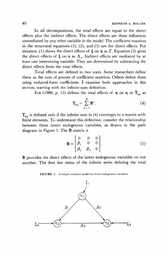
Tn is defined only if the infinite sum in (4) converges to a matrix with finite elements. To understand this definition, consider the relationship between three latent endogenous variables, as drawn in the path diagram in Figure 1. The B matrix is

0 0 0 B= 1 0 0 . (5)

2 /33 0

B provides the direct effects of the latent endogenous variables on one another. The first few terms of the infinite series defining the total

FIGURE 1. A simple recursive model for three endogenous variables.

'i


TOTAL, DIRECT, AND INDIRECT EFFECTS 41

effects of T1 on Tr are

T = B + B2 + B3 +

O O O O O (6) = , 0 0 + 0 0 0 +0+ ...

f2 i3 0 _13) 0 0

Clearly, since all Bk for k > 3 equal zero, the series converges and the total effects are defined. The first term in the series represents the direct effects of X1 on i1. The second and higher-power terms represent the indirect effects of varying lengths. In Figure 1, the only indirect effect of length 2 is , j83, the influence of ql on 73 mediated by l2. The zero values for B3 and the higher-power terms indicate that all indirect effects of length 3 or greater equal zero. Summing the right-hand side of (6) gives

0 0 0

T,,= 3 A 0 0 . (7) _2 +tjM13 3 0

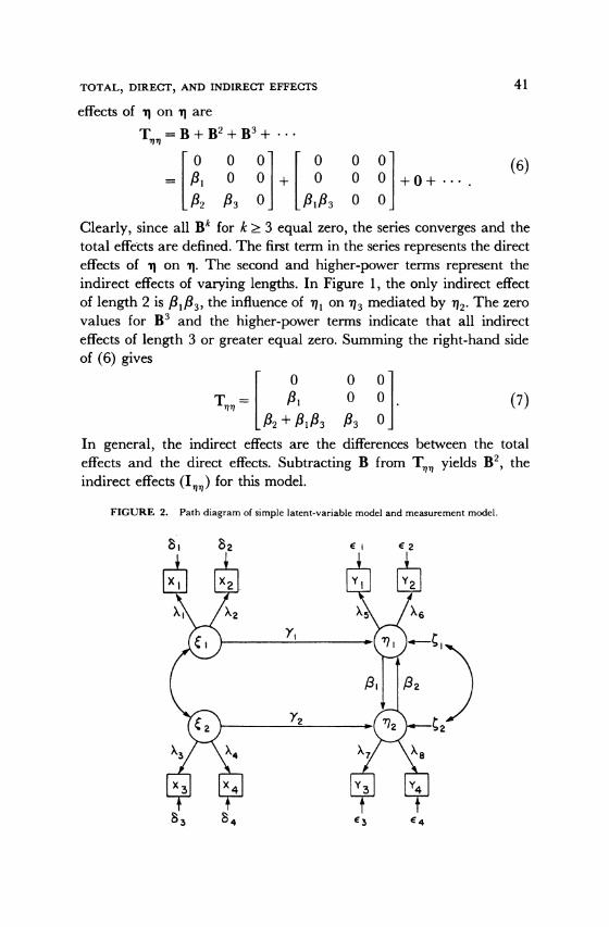
In general, the indirect effects are the differences between the total effects and the direct effects. Subtracting B from T,, yields B2, the indirect effects (I,,) for this model.

FIGURE 2. Path diagram of simple latent-variable model and measurement model.

This result generalizes. For recursive systems in which B can be written as a lower triangular matrix, Bk equals zero for k > m (where m is the number of q 's). Thus, B converges and the total effects are defined. These total effects equal Em-l' Bk. It then follows that the indirect effects are Tn

- B, or -m=2 Bk. Nonrecursive models are more complicated. Consider the exam-

ple in Figure 2:

B= 1 1o2] B-[? r'}.

(8)

where i,B represents the direct effect of 17 on 92 and 12 represents the direct effect of 72 on 1. The indirect effects of T on q of particular lengths can be determined by raising B to the appropriate powers. The indirect effects for lengths 2, 3, and 4 are

B2= Pf1f2 0

B4= 08,

0

B 2 0 ]

22 2

Unlike Bk in recursive models, Bk in nonrecursive models is not

necessarily zero for k > m. Also, as B2 and B4 illustrate, an endogenous variable can have an indirect effect on itself. For instance, , changes 12 by P1 units, but the PI change in T2 leads to a /f/I2 shift in j1. To

determine the total effects, T,,, we let k - coo and sum all Bk:

OC x

T,= L Bk= x k=l E iL(j-1 )

j=l '=1

E= ( Ei(Z()a(

= 1

L (3I12) 2 E (1 ) j=1 i=l

(10)

Each element of T, involves an infinite sum. For instance, the (1,1)

(9)



element is

00

Z (9Il2)i= 3112 + (132)2+ (2 132)3 + ** (ii) i=1

The total effect of j1 on itself is defined if (11) converges. To determine the conditions for convergence and the value to which it

converges, first add (P,132)? to both sides of (11): 00

E (PIP2)Y= (13I2) + (P12)1 + (1332)2 + * . (12) i=0

Equation (12) is a geometric series. For this series to converge, (13112)' must go to zero as i approaches infinity. This occurs only if 1f i 121 is less than one.

To find the convergent value, multiply the right-hand side of

(12) by (1 - 1312):

(1 - 13 (2)(1 + 1332 + (132)2 + .* * + (1l2)i) = 1 - (213i2)+l.

(13)

Since 11l1,21 is less than one, (#l,#2)i+ goes to zero as i goes to infinity. This leaves one on the right-hand side of (13). For the product on the left-hand side to equal one, (1 + P12 + (31132)2 + ... +(332)i) (1 - 1 2) -

1 as i oo. Thus, 00

E (f1 Y=2)= (1- -

2)Y1 for 11821 < 1 and i- o. (14) 0=o

To obtain the original series in equation (11), subtract 1(= (l3,12)0)

from both sides of (14): oo

E0 1A i 313 (15) i=l 1

-- PIPl2

This is the convergent value for equation (11) and the total effect of 1 on itself. To sum up, if 131f321 < 1, the (1,1) element of (10) converges to 1i1i2/(1 - f1fi2). Since the (1,1) and (2,2) elements are identical, the (2, 2) element also converges to this value. When we apply a similar argument to the other elements of (10), we see that under the same condition of f1,81i 21 < 1, the (1,2) element converges to 32/(1 - 3112) and the (2,1) element converges to Al/(1 - 1312). Thus, the total

43

effects of X on TI are

T 1 P12 2 T, = ZB =(11,132)) 12 (16) k=1 L 1 P1P-2J

and the indirect effects are

I,,r,=T-,,,,B=(1-/12) [ 122 1 2] (17) [/l12 P132J

If l/3l121 equals or exceeds unity, then the total and indirect effects

among the latent endogenous variables in Figure 2 are not defined. In general, for the total effects T,, (= EI= Bk) to be defined, Bk

must converge to zero as k -* oo (Ben-Israel and Greville 1974). The matrix is convergent if and only if the modulus or absolute value of the

largest eigenvalue of B is less than one (Bentler and Freeman 1983, p. 144).2 To continue the generalization of the previous results, we next search for the value to which T, converges. First, we add I (= B?) to

T,n and then premultiply the sum I + B + B2 + . - + Bk by (I- B):

(I- B)(I + B + B2 + * + Bk) = I- Bk+l. (18)

Since Bk+ - 0 as k -oo, the last term in (18) approaches zero,

leaving I. For the product of the two left-hand terms in (18) to equal I, (I + B + B2 + * +BBk) must converge to (I- B)

- as k - oo. If I is

subtracted from this value, T,, results:

Tn, = (I- B)- -. (19)

The indirect effects are

I,, = (I- B)- - I - B. (20)

The above shows the decomposition of effects for the latent

endogenous variables on one another using the infinite-sum definition.

Decompositions of the latent exogenous variables on the latent endogenous variables are closely related. Following Bentler and Freeman

(1983, p. 143), we can determine the total effects of t on 1 by

2 The similar canonical form of B is useful in studying Bk and in under-

standing the justification for placing this condition on the eigenvalues of B. See Searle (1982, pp. 282-89) and Luenberger (1979) for further discussion.



repeatedly substituting equation (1) for ri into the right-hand side of

(1):

-= Bi +r +

= B(Bq + rE + ) + rP + = B2i + (I + B)(rF + {) = B2(BI + rt + ) + (I + B)(rt + ) (21) = B3l + (I + B + B2)(F + {)

= B*k + (I + B + B2 + ... + Bk-)(r + ).

The total effects of t on 1 are in the coefficient matrix for t in the last line of (21): (I + B + B2 + *- +Bk-')r. The (I + B + B2 + * * +B*-1) term is an infinite sum that converges to (I - B) -1 under

the same conditions stated above. That is, the absolute value or modulus of the largest eigenvalue of B must be less than one. The T,} matrix under this condition is

T, = (I- B)-'F. (22)

Since the direct effects of t on T1 are in r, the indirect effects of t on T are

I (=(I-B)-F- r = ((I- B) 1-)l)r. (23)

Equation (23) shows that the indirect effects of t on T equal the

product of the total effects of rl on 11 and the direct effects of t on tI. The derivation of the total and indirect effects of i on y follows

a similar strategy. Repeated substitution of equation (1) for T1 in the measurement equation for y yields

y = AyBk*, + Ay(I + B + B2 + * - . + Bk- l)

(24) +A (I+B+B2+ *- +Bk-'1)+e.

For convergent B, the total effects Ty are

Tyf =Ay(I- B)-Ir. (25)

45

The indirect effects also equal (25), since t has no direct effects on y.3 By the same logic, the total effects of '1 on y are

T, =A (I+B+B2 + +Bk) (26)

= Ay(I- B)-,

and the indirect effects are

Iy = Ay(I - B)-' - Ay= A((I - - I). (27)

Total and indirect effects are defined only under certain conditions, i.e., when the absolute value or modulus of the eigenvalues of B is less than one.4 The eigenvalues are not always readily available. However, two shortcuts can identify convergent B. I have already discussed the first: If B is a lower triangular matrix, then Bk is zero for k > m. The second applies to nonrecursive models: If the elements of B are positive and the sum of the elements in each column is less than one, the absolute values of the eigenvalues are less than one (Goldberg 1958, pp. 237-38). This is a sufficient condition, but it is not necessary for

stability. Given its ease of calculation, it should prove useful in many situations.

The preceding approach defines the total effects as infinite sums of functions of the coefficient matrices, and it requires that stability conditions be met for these effects to exist. A second strategy uses reduced-form equations to identify total effects (Alwin and Hauser

1975; Fox 1980, p. 25; Graff and Schmidt 1982). In classical econometric models, reduced form refers to solutions of structural equations in which all endogenous variables are written as functions of only exogenous (or predetermined) variables, structural coefficients, and dis- turbances. My use of the concept of reduced forms is similar to Graff

and Schmidt's (1982). It differs from the classical econometric concept in that i, the vector of exogenous variables, is a vector of latent variables rather than directly observed variables.

3J6reskog and Sorbom (1981, p. 39; 1982, p. 409) incorrectly list the direct effect of i on y as Ay and the indirect effects as AY(I

- B)- F - Ayr. Freeman

(1982), in his dissertation, also notes this error. 4 This condition is also necessary for the existence of T,,, but it is not

necessary for the existence of Ty,, Ty1, and T, (see Sobel 1986, p. 166). In

practice, we would rarely, if ever, be interested in these latter total effects if T,, did not exist.



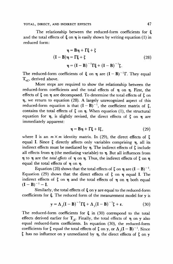
The relationship between the reduced-form coefficients for i and the total effects of t on aq is easily shown by writing equation (1) in reduced form:

T = Bq + rF +

(I - B)n = rt + t (28)

on = (I- B)-'r + (I- B)-1 .

The reduced-form coefficients of t on a are (I- B) -1. They equal T.f, derived above.

More steps are required to show the relationship between the reduced-form coefficients and the total effects of l on Tq. First, the effects of t on X are decomposed. To determine the total effects of S on TI, we return to equation (28). A largely unrecognized aspect of this reduced-form equation is that (I- B)-1, the coefficient matrix of g, contains the total effects of t on T. When equation (1), the structural equation for 71, is slightly revised, the direct effects of { on 11 are immediately apparent:

X1 = Bi + rQ + It, (29)

where I is an m X m identity matrix. In (29), the direct effects of C

equal I. Since t directly affects only variables comprising T1, all its indirect effects must be mediated by 1. The indirect effects of S include all effects from a (the mediating variable) to rj. But all influences from TI to 1 are the total effects of al on -. Thus, the indirect effects of S on a

equal the total effects of X1 on -i.

Equation (28) shows that the total effects of S on q are (I - B)- . Equation (29) shows that the direct effects of S on T1 equal I. The indirect effects of S on 1 and the total effects of 1 on l both equal (I- B)- - I.

Similarly, the total effects of t on y are equal to the reduced-form coefficients for 1. The reduced form of the measurement model for y is

y = A,(I - B) - rF + A(I - B) -{ + E. (30)

The reduced-form coefficients for t in (30) correspond to the total effects derived earlier for Ty. Finally, the total effects of Ta on y also equal reduced-form coefficients. In equation (30), the reduced-form coefficients for { equal the total effects of ; on y, or Ay(I - B)-1. Since S has no influence on y unmediated by -q, the direct effects of { on y

47

are zero, and the indirect and total effects are equal. The indirect effects of 1 on y are all the influences that T exerts on y; therefore, Ty is A (I - B) -. Thus, when the reduced-form and structural equations are used, all the total and indirect effects can be identified.

Defining total effects as the sum of an infinite series and

defining them in terms of reduced-form coefficients appear to yield the same results. However, there is one important difference. To illustrate, consider T . For the total effects E k=Bk to be defined, the conver-

gence condition for B must be met. To write the structural equation for

i1 in reduced form, (I - B)-1 must exist. The existence of (I- B)-' need not imply the convergence condition. For example, specify B as

B=[ 0 ] (31)

The matrix (I - B) is nonsingular with an inverse of 1 1 2]

(I-B)1 =- ]. (32)

Nevertheless, IPf, ,i21 (= 4) exceeds one, so the convergence condition is not met. In this example, the total effects would be defined by the reduced-form coefficients, although they would be nonexistent because of the convergence criterion. In such a situation, it is questionable whether the reduced-form coefficients can be interpreted as total effects. Since the convergence condition is sufficient for (I - B)-1 to exist (Goldberg 1958, p. 238), it makes sense to require convergence even if the decomposition of effects is approached via reduced-form

equations. To illustrate the decomposition, I again refer to Figure 2. Here,

l and 52 are latent exogenous variables, ml and T2 are latent

endogenous variables, and there are two indicators each for , , 12, 1,l

and T/2. The matrix representation for the latent variable model is

N::1-[? 1[::1? ^ h T'l ++H (33)

12 K 0 [jq ][Y2 [42] J2Y The equations for the measurement models are

x,- A, 0O ~1 x1

X3 = 0X A [ A+ 2 (34)

X4- 0 8 4- 4~



and

y,~ X5 0 e

Y2 X6 _ 0 rl +2 -

+ .(35) Y3 0 7 2 3 * (35)3

Y4. 0 X8 -4-

In equations (9) through (16), I derived the total, direct, and indirect effects of q1 on r for this model. I now do the same for the effects of t on 1l. According to the formula above, the total effects of t on '1 equal (I - B)- 1. When this result is applied to the model shown in Figure 2, we get

T, -(I-B) -r (1-=A) [:2 l 1 ][ y]

(36) -(i A2) 11Y1 [ 2Y2 ]

The first term on the right-hand side of this expression, (1 - fi1 2)-1, results from the reciprocal relationship between 71 and 21, which may be activated by the effect of ^l (or 2) on 'll (or q2)' For this feedback

loop to converge, 1Af21 must be less than one. The direct effects of t on aq appear as coefficients in F. The indirect effects of t on 1 equal ((I - B)-1 - I)r, which for Figure 2 are

I,}=(i-= (- 3) 1 :)l [1 2Y2Y

(37)

Similarly, the total and indirect effects for the remaining variables can be determined by substituting the B, F, and Ay in Figure 2 into the

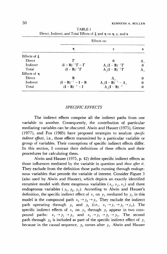
appropriate decomposition formula derived above. Table 1 summarizes the decomposition of effects for the general

structural equation model with latent variables. It is well known that the classical econometric simultaneous equation model, confirmatory factor analysis, and the MIMIC model are special cases of the LISREL model (Joreskog and S6rbom 1982; Joreskog and Goldberger 1975). Thus, Table 1 can be applied to these models given the appropriate substitutions. For example, if x were substituted for i, and y for al, the decomposition of effects in Table 1 would match those in Fox (1980), except for a slight difference in notation.

49

TABLE 1 Direct, Indirect, and Total Effects of E and n on XI, y, and x

Effects on:

1 y x

Effects of i

Direct r 0 A, Indirect (I-B)-r- r Ay(I-B)-r 0 Total (I - B)- Ay(I - B)- A,

Effects of ii

Direct B Ay 0 Indirect (I-B)- '-I-B A,(I- Bf)- -Ay 0 Total (I-B)- -I Ay(I-B)-1 0

SPECIFIC EFFECTS

The indirect effects comprise all the indirect paths from one variable to another. Consequently, the contribution of particular mediating variables can be obscured. Alwin and Hauser (1975), Greene

(1977), and Fox (1985) have proposed strategies to analyze specific indirect effects, i.e., those effects transmitted by a particular variable or

group of variables. Their conceptions of specific indirect effects differ. In this section, I contrast their definitions of these effects and their

procedures for calculating them. Alwin and Hauser (1975, p. 42) define specific indirect effects as

those influences mediated by the variable in question and those after it.

They exclude from the definition those paths running through endogenous variables that precede the variable of interest. Consider Figure 3

(also used by Alwin and Hauser), which depicts an exactly identified recursive model with three exogenous variables (x1, x2, x3) and three

endogenous variables (y, Y2, Y3). According to Alwin and Hauser's definition, the specific indirect effect of xl on Y3 mediated by Y2 in this model is the compound path x, - Y2 -* y3. They exclude the indirect

path operating through y, and Y2 (i.e., x -y-*Yl - -Y2 3). The

specific indirect effects of xl on Y3 through y, appear in two com-

pound paths: x~~y~ - Y 3 and x,- y-y Y2 *-> 3. The second

path through y2 is included as part of the specific indirect effect of y, because in the causal sequence, Y2 comes after yl. Alwin and Hauser



FIGURE 3. Alwin and Hauser's (1975) recursive model.

X23Y3

conceptualize specific indirect effects as increments in the causal se-

quence of variables in a model. I call these indirect effects incremental

specific efects. Incremental specific effects are restrictive, i.e., they do not

include compound paths operating through prior endogenous variables. Greene's (1977) idea of specific effects is even more restrictive. It includes as specific effects only those influences mediated by the

intervening variable or variables of interest.5 For instance, according to his definition, the specific effect of x1 on y3 operating through Yl is the

compound path x1 - yI ->Y3 (see Figure 3). This differs from the incremental specific effects for Yl because it excludes the path going through Y2 (i.e., x, -, y - y 32 3). Greene's notion of specific indirect effects focuses on those effects that operate through Yl but no other

endogenous variable. Alwin and Hauser's concept of incremental

specific effects includes all compound paths subsequent to the endogenous variable of interest. I call Greene's specific indirect effect exclusive

specific effects.

5 Greene's (pp. 377-78) emphasis is on presenting a computational method for computing specific effects for recursive systems. He does not give a detailed definition of specific effects nor does he explain how his use of the term differs from Alwin and Hauser's. Greene's computation method suggests a particular definition of specific effects, which is what I discuss.

51

Fox's (1985) definition of specific effects is more inclusive than Greene's or Alwin and Hauser's. Fox defines a specific indirect effect as all compound paths that traverse a particular intervening variable. For instance, Fox's definition implies that the specific effect of xi on )3 through Y2 consists of two compound paths: x1 -> y, -Y2 y-3 and xl -Y2 y3 (see Figure 3). The incremental and the exclusive specific effects in this case include only a single path: xl -o Y2 -Y3. According to Fox's definition, the specific effect of x1 on Y3 by way of y, incorporates x~ -Yl -Y3 and x~ -yl -y2 ->Y3. The incremental specific effect is identical to this, but the exclusive specific effect is not. The latter is composed of a single path: xi -'yl --y3. Fox includes as specific indirect effects all paths coming into or going out of a particular variable. I call these inclusive specific efects.

Each definition of specific indirect effects is tied closely to a particular method for decomposing effects. Alwin and Hauser (1975, p. 42) summarize their procedure as follows:6

For each endogenous (dependent) variable in the model, obtain the successive reduced-form equations, beginning with that containing only exogenous (predetermined) variables, then adding intervening variables in sequence from cause to effect. The total effect of a variable is its coefficient in the first reduced-form equation in which it appears as a regres- sor.... Indirect components of effects are given by differences between coefficients of a causal variable in two equations in the sequence, where the mediating variable (or variables) is that which appears as regres- sor in one equation and not in the other. However, it must be understood that indirect effects so computed will include those mediated by the intervening variable(s) in question and later variables.

Greene's procedure, unlike Alwin and Hauser's, requires matrix manipulations. The first step is to form a square matrix with a row to represent each variable and a column to do the same. If one variable

6 Their procedure is designed for exactly identified, recursive models.



affects another, its coefficient is listed in its row and in the column of the variable it affects. To determine an exclusive specific effect, the rows and columns corresponding to endogenous variables other than those of interest are first removed, creating a new and smaller square matrix. This new matrix is premultiplied by itself again and again until the resulting matrix is null. When each matrix product, beginning with the first, is summed, the end result is a matrix of the exclusive specific effects.

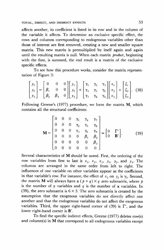
To see how this procedure works, consider the matrix representation of Figure 3:

Yl 0 0 0 Yl Yi 72 73 X1 '1

Y2 = Al 0 Y 4 75 + 42 . (38)

Y3 _2 3 0 Y3 77 Ys 9s X3 J3

Following Greene's (1977) procedure, we form the matrix M, which contains all the structural coefficients:

0 0 0 y1 y, Y7

O 0 0 Y2 75 78

O O O 3 Y, 79 , [0 I'] (39) o0 0 0 0 1 2 [0 B' i3 00 0 0 0 0 3

0 0 0 0 0 _

Several characteristics of M should be noted. First, the ordering of the row variables from first to last is x1, x2, x3, y, Y2, and Y3. The columns are arranged in the same order from left to right. The influences of one variable on other variables appear as the coefficients in that variable's row. For instance, the effect of x2 on Y2 is 75. Second, the matrix M will always have a (p + q) x q zero submatrix, where p is the number of y variables and q is the number of x variables. In (39), the zero submatrix is 6 X 3. The zero submatrix is created by the assumption that the exogenous variables do not directly affect one another and that the endogenous variables do not affect the exogenous variables. Third, the upper right-hand corner of (39) is F', and the lower right-hand corner is B'.

To find the specific indirect effects, Greene (1977) deletes row(s) and column(s) in M that correspond to all endogenous variables except

53

those whose exclusive specific effects he wants to estimate. He also

keeps the rows and columns of the exogenous variables. To determine the exclusive specific effect of xl on Y3 mediated by Yl, he removes the row and column corresponding to Y2, the only other intervening variable in the model. Thus, he forms M* by removing the fifth row and fifth column from M:

0 0 0 y, y7

0 0 0 Y2 Y8

0 0 0 0 2

M*= O O O '3 59 ' (40)

?0 0 0 0

Next, he premultiplies M* by itself, yielding

0 0 0 0 Y1I2 0 0 0 0 Y2fi2

M*2^ =0 0 O O y/A2 (41)

0000 0 0000 0

As is easily verified, further premultiplication will result in a matrix of zeros. Therefore, the only nonzero matrix in the sum of product matrices is (41). Thus, the element in the first row and last column of M*2 gives the exclusive specific effect of x, on y, through Y,. In this case, this effect equals Y/l2.

In recursive systems with even a moderate number of endogenous variables, Greene's procedure may generate a number of terms to

multiply and sum. Furthermore, his discussion and examples of exclusive specific indirect effects do not treat nonrecursive systems. Recently, Fox (1985) proposed a procedure for deriving inclusive specific indirect effects that is computationally similar to Greene's method but avoids the summing of a power series of matrices. It is also more general than either Greene's or Alwin and Hauser's methods. Fox assumes a classical econometric model in which x = - and y = T. Computations start with

TV,x the total effects of x on y, formed as (I - B)-l. From T,x he deletes the row(s) of the variable(s) whose specific effects he wishes to

analyze. Next, he removes the row(s) and column(s) of B and the

row(s) of r corresponding to the variable(s) of interest, leading to F*



and B*, where the "*" indicates the matrices with the proper row(s) or

column(s) absent. Then, he forms a new total effects matrix, (I* - B*)-'1*. He subtracts the (I* - B*)-1'* matrix from the original Tyx matrix with the appropriate row(s) removed to determine inclusive specific effects through the variable(s) being analyzed.7 He follows a similar series of steps to find the inclusive specific effects of y on y.

A generalization of specific effects. The procedures reviewed above share one limitation: They are oriented toward variables rather than

paths. Suppose we want to know that part of the indirect or total effects transmitted by a path or combination of individual paths. The preceding methods would be helpful only if these paths happened to corre-

spond to incremental, exclusive, or inclusive specific indirect effects. This need not be the case, of course. In this subsection, I explain a

technique that is coefficient (or path) oriented. Since the coefficient or

path is a more elementary unit than the variable, this procedure is more general than the existing procedures. By choosing appropriate combinations of paths, we can determine the specific indirect effects of variables. In the next few pages, I use this idea to show that the specific indirect effects proposed by Alwin and Hauser, Greene, and Fox are

special cases of effects estimated with this alternative method. Then, I

apply this method to a type of specific effect that falls outside the scope of these other procedures. Unlike Alwin and Hauser's procedures for

estimating specific indirect effects, this method is not restricted to

exactly identified recursive models nor to incremental specific effects. Like Greene's and Fox's procedures, it uses matrix operations; but unlike their procedures, it does not require row and column removal.

The method has several steps. The last is optional.

1. Identify the changes needed in the coefficient matrices. 2. Modify the coefficient matrices. 3. If B is changed, check the modulus or absolute value of the largest

eigenvalue of the new B to insure that it is less than one. 4. Calculate the direct, indirect, or total effects with the modified

matrices. 5. Subtract the new decompositions from the old.

7 Fox also shows how Alwin and Hauser's incremental specific effects can be computed with his procedure.

55

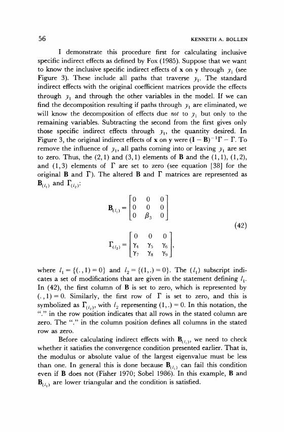
I demonstrate this procedure first for calculating inclusive specific indirect effects as defined by Fox (1985). Suppose that we want to know the inclusive specific indirect effects of x on y through y, (see Figure 3). These include all paths that traverse y1. The standard indirect effects with the original coefficient matrices provide the effects

through y, and through the other variables in the model. If we can find the decomposition resulting if paths through y, are eliminated, we will know the decomposition of effects due not to y, but only to the

remaining variables. Subtracting the second from the first gives only those specific indirect effects through y,, the quantity desired. In

Figure 3, the original indirect effects of x on y were (I - B) -r - r. To remove the influence of y,, all paths coming into or leaving y, are set to zero. Thus, the (2,1) and (3,1) elements of B and the (1,1), (1,2), and (1,3) elements of F are set to zero (see equation [38] for the

original B and F). The altered B and F matrices are represented as

B(/,) and r(2):

0 0 0

B()= 0 0 0 0 /33 0

(42) 0 0 0

r(/2)= Y4 Y5 Y6 Y7 Y8 Y9

where 1 = {(., 1) = 0} and 12 = {(1,.) = 0}. The (11) subscript indicates a set of modifications that are given in the statement defining /1. In (42), the first column of B is set to zero, which is represented by (., 1) = 0. Similarly, the first row of r is set to zero, and this is

symbolized as Fr2), with 12 representing (1,.) = 0. In this notation, the "." in the row position indicates that all rows in the stated column are zero. The "." in the column position defines all columns in the stated row as zero.

Before calculating indirect effects with B(, ), we need to check whether it satisfies the convergence condition presented earlier. That is, the modulus or absolute value of the largest eigenvalue must be less than one. In general this is done because B(/) can fail this condition even if B does not (Fisher 1970; Sobel 1986). In this example, B and

B(/I) are lower triangular and the condition is satisfied.



The indirect effects Iyx based on the original B and F (see [38]) are

(I-B)-'F- =

fiYi i(Y2 1Y3

(32 + PI33)Y1 + f3Y4 (32 + 1i3)Y2 + ?3Y5 (32 + 31/3)Y3 + P3Y6

(43)

The indirect effects based on the B(1,) and F(12) of (42), in which those paths into or out of y, have been eliminated, are

0 0 0

(I-B(1) I2)-(2= 0 0 0 . (44) Bi374 3Y75 f3Y6

Equation (44) reveals that the indirect effects of x on y that remain after those passing through y, have been eliminated are limited to indirect effects of x on Y3 operating through Y2. Subtracting (44) from

(43) produces the inclusive specific effects of yi:

0 0 0

flY,I f1Y2 l1Y3 . (45)

(2 + 133)Y1 (2 + 1/i3)Y2 (2 + ?1f3)Y3

These results match those obtained using Fox's (1985) procedure. In

general, to calculate inclusive specific effects, we first form the indirect effects with the original matrices. Second, we alter the B and r matrices so that all paths leading to or from the variable or variables of interest are set to zero. Third, assuming that the new B meets the convergence condition, we recalculate the indirect effects with these modified matrices. Finally, we subtract the modified indirect effects from the original effects to obtain the inclusive specific effects.

Greene (1977) limited his discussion of exclusive specific effects to recursive models with observed variables. The alternative procedure I have proposed can handle exclusive specific effects for these types of models and for nonrecursive or latent variable models. The first step is to determine the changes needed in the coefficient matrices for exclusive specific effects. Greene's specific effects include only those paths through a particular endogenous variable. Excluded are paths to the

57

selected endogenous variable from the other endogenous variables. Also excluded are the paths from the exogenous variables to the endogenous variables not of interest. All columns of B are set to zero except those representing the influence of the endogenous variable(s) whose exclusive specific effects are to be calculated. This modification forces to zero the direct effects of the excluded endogenous variables. For F, all rows are set to zero except those corresponding to the effects of the exogenous variables on the endogenous variable(s) selected. The indirect effects are formed using these modified matrices. The equation for indirect effects is computed by substituting the modified matrices for the original matrices. This creates exclusive specific effects. An example will help clarify this procedure.

In Figure 3, suppose that we want to know the exclusive specific indirect effects of Yl The modified B and F are

0 0 0 Y1 Y2 Y3

B(,)0= , 0 0 r(2)

0 0, (46)

2 0 0 0 0 0

where I/=((.,2)=0, (.,3)=0} and 12={(2,.)=0, (3,.)=0}. The

only nonzero elements in B(l,) appear in the first column and represent the direct effects of y, on Y2 and Y3. The nonzero elements in r(l2) denote effects of the exogenous variables on y. The modified versions of the coefficient matrices replace the original matrices in the indirect effects formula, yielding

0 0 0

(I- B(,,) -r12)- r(2)= 1IYI1 17Y2 /,Y3 . (47)

fiY21 f2Y2 A2Y3

As the first row of (47) shows, x has no exclusive specific indirect effects on y1; all its effects are direct. The second row contains the specific effects of x on Y2 exclusively through y,, and the third row contains the exclusive specific effects of x on Y3. The procedure illustrated above can be applied to other types of models and can be used to find the exclusive specific effects of more than one endogenous variable at a time.8

8 Alwin and Hauser's (1975) incremental specific effects can also be calculated with this method. However, these effects are not clearly defined when a nonrecursive model is analyzed because with a feedback or reciprocal relationship, it is unclear which variable precedes or follows in the causal hierarchy.



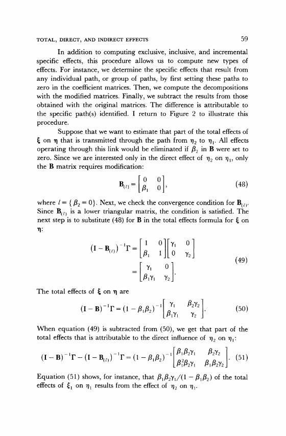
In addition to computing exclusive, inclusive, and incremental

specific effects, this procedure allows us to compute new types of effects. For instance, we determine the specific effects that result from

any individual path, or group of paths, by first setting these paths to zero in the coefficient matrices. Then, we compute the decompositions with the modified matrices. Finally, we subtract the results from those obtained with the original matrices. The difference is attributable to the specific path(s) identified. I return to Figure 2 to illustrate this

procedure. Suppose that we want to estimate that part of the total effects of

on '1 that is transmitted through the path from %2 to 1 . All effects

operating through this link would be eliminated if /2 in B were set to zero. Since we are interested only in the direct effect of T2 on / 1, only the B matrix requires modification:

B(, [ 0 (48)

where / = { f2 = 0}. Next, we check the convergence condition for B(t). Since B(/) is a lower triangular matrix, the condition is satisfied. The next step is to substitute (48) for B in the total effects formula for t on

1:

(49)

~lB Y2 '

The total effects of t on 1t are

(I-B)- r=( - 2) [Yi 12Y21 (50)

When equation (49) is subtracted from (50), we get that part of the total effects that is attributable to the direct influence of '2 on / 1:

(I- B)-lr- (IB(l,)) r=(l-l( 2)- [f ,f2?1 2( ]. (51)

Equation (51) shows, for instance, that //lfl2Y/(l -

f1I2) of the total effects of (l on /l results from the effect of 112 on 1,.

59

The decompositions I have discussed can be calculated in several

ways. The formulas in Table 1 can be programmed using software that has matrix capabilities. For instance, APL, GAUSS, the PROC MATRIX procedure in SAS, or SAS/IML can perform the required matrix algebra. The alternative is to use LISREL V or VI. Each of these versions calculates the estimated total effects of 5 and 'l. The estimated direct effects are the structural coefficients in Ax, A y, , and B. The indirect effects can be obtained by subtracting the direct effects from the total effects. Finally, for simple models, the decomposition of effects can be calculated with a hand calculator when the structural coefficient estimates are available. The more complicated the model, the less practical is this option.

ASYMPTOTIC VARIANCES OF EFFECTS

So far, I have limited my discussion to methods of decomposing various types of effects. Once these effects are in hand, the question of their statistical significance arises. This section briefly describes the means of obtaining estimated asymptotic variances and tests of significance for all types of effects.

The asymptotic variances of the direct effects are readily available for maximum likelihood (ML) estimators when y and x have multinormal distribution (Joreskog 1978, p. 447) and for generalized least squares (GLS) estimators under suitable conditions (Browne 1984). Significance testing of the indirect, total, and specific effects is more

complicated, since it typically involves obtaining the variances of

products of coefficient estimates. For instance, we can estimate the

asymptotic variance of an ML estimator of a direct effect (e.g., /), but the asymptotic variance of an indirect effect (e.g., flxh) is less straight- forward. The multivariate delta method (Bishop, Fienberg, and Holland 1975, pp. 486-500; Rao 1973, pp. 385-89) proves helpful in this situation. The delta method begins with the assumption that a

parameter estimator has an asymptotically normal distribution with a mean of the parameter and an asymptotic covariance matrix. It then

provides a method of estimating the asymptotic covariance matrix of functions of the parameter.

Folmer (1981, pp. 1440-42) and Sobel (1982, 1986) suggested

applying the delta method to estimate the asymptotic variances of



total, indirect, and other types of effects. The procedure is as follows. First, define 0 as an s-dimensional vector of the unknown elements in B, r, and Ay, and define oN as the corresponding sample estimator of 0 for a sample of size N. Choose an estimator so that ON has an asymptotically normal distribution with a mean of 0 and an asymptotic covariance matrix, N-'V(0). Under appropriate assumptions, the ML and GLS estimators of 0 satisfy these conditions (Joreskog 1978, p. 447; Browne 1984).

Next, define an r-dimensional vector f(0) that is a differentiable function of 0. In this case, f(0) contains the indirect (or total) effects that are functions of the direct effects. Under these conditions, the multivariate delta method states that the asymptotic distribution of

f(ON) is normal, with a mean of f(0) and an asymptotic covariance matrix of N- ( f/dO)'V(0) ( f/d0).9 The first row of af/0e is

df,/dl,, af2/a01,..., afr/O,, where f/ is the ith element of f(0). The second row is df,/d02, af2/ 02,..., dfr/O 2, and so on, so that

f/dO is an s x r matrix. For large samples, ON is substituted for 0 to obtain an estimate of the asymptotic covariance matrix for f(ON):

__9 'a / df _"Ij (df J ( f j (52)

To illustrate this procedure, consider the simple casual chain model:

T1 = Y1ii +

~2 = '1'1 + ~2' 312 h8171 + ~2 ~(53)

In (53), assume that l, and '2 are uncorrelated with each other and with ~,, that E('i) is zero, and that /1, 2, and l, are deviated from their means. Define y,fi, the indirect effect of ~l on 12, as the single element of f(O), with 0 containing y, and p,. The df/0O is [/P, y,]',

9 In addition to requiring a consistent and asymptotically normal estimator of 0, f(O) must be continuously differentiable with respect to 0 in the neighborhood of the true parameter, and I assume the continuity of N-1V(0) with respect to 0 in the neighborhood of the true parameter. See Bishop et al. (1975) for additional discussion of these conditions.

61

and the asymptotic covariance matrix of the estimator of 0 is

N-V(J) v( I (54)

The main diagonal of (54) contains the asymptotic variances of Y1N and ,BN. The off-diagonal elements are zero, since these two coefficients are uncorrelated in a recursive system. When these matrices are combined using the multivariate delta method, the asymptotic variance of y,i/l is the scalar:

^I [ 2V(-y) + yl V(#i)]. (55)

If /, and Y1 are zero, the delta method cannot be applied. Otherwise, by substituting the sample estimates into (55), we can obtain an estimate of the asymptotic variance of 'YIvN/1 for large samples.

Considering each element of the indirect (or total) effects in the above fashion for more complicated models is extremely tedious. Sobel

(1986) proposes a matrix formulation that is a far more efficient means of finding df(O)/dO, which is required for the covariance matrix of

f(O). In the appendix, I list the df(O)/d0 for the indirect effects and use them to estimate the standard errors of effects reported in the next section.

EMPIRICAL ILLUSTRATION

To illustrate the preceding methods, I utilize a model relating objective and subjective components of stratification for individuals.

Figure 4 depicts this model. Define xl as income, x2 as occupational prestige, -/l as subjective income, r7, as subjective occupational prestige, and 773 as subjective overall class ranking. Let yl, Y2, and Y3 be measures of the 771, 12, and r/3 latent variables. In the model, subjective income (/1)) and subjective occupational prestige (772) are

dependent upon their objective counterparts and are reciprocally related to each other. In turn, the subjective income and occupation variables (7q1 and /2) have direct effects on overall subjective class

(173). The data are taken from a white subsample of 432 individuals from Indianapolis, Indiana (Kluegal, Singleton, and Starnes 1977).



FIGURE 4. A model of objective and subjective stratification.

E }I EI

i E2

The ML estimates based on the covariance matrix of these five variables give

0 .288 0

(.168) .101 0

.330 0 0 (.016) B= (.090) r= 0 .007 . (56)

.399 .535 0 (001)

(.139) (.201) - ? ?

The standard errors are in parentheses. All coefficient estimates carry the expected positive signs, and all are statistically significant (p < .05, one-tailed test), though /? is barely significant. The goodness of fit of the overall model is excellent (X2 = 0.27, df= 1, GFI = 1.00, AFGI =

.996). The estimated indirect effects of 'q on '1 and x on 1 are10

.105 .030 0 .011 .0022

(.067) (.036) (.006) (.0014) .035 .105 0 . 037 .0007 (

T1q (.026) (.067) (.011) (.0004) (57)

.237 .183 0 .064 .0048

(.105) (.127) (.013) (.0014) 10 In this model, x is equivalent to i, and Iy, and I.x are of little interest,

since AY is an identity matrix. Also, the estimate of the eigenvalues for B are

considerably less than one. Therefore, the convergence condition is met.

63


In the I1x matrix, all the indirect effects of x on q except the indirect effect of occupational prestige (x2) on subjective income (71l) are

statistically significant (p < .05, one-tailed test). In the IT, matrix, in

contrast, none of the indirect effects of T] on i1 except the effect of

subjective income (-/1) on subjective overall class (7q3) are statistically significant. This suggests that with one exception, the most significant effects of the subjective variables on one another are direct, not indirect. Statistically significant direct effects need not be accompanied by significant indirect effects.

To explain the largely nonsignificant indirect effects of q1 on q, we can begin with ,l, the coefficient of the path from subjective occupational prestige (r2) to subjective income (Xq1). Relative to 2,, the influence of subjective income on prestige, /l is somewhat weak. In substantive terms, people who perceive their income as high are likely to perceive their occupational prestige as higher than those who

perceive their income as low. Yet, individuals with positions they perceive as prestigious are less likely to believe that their incomes are

high. Since the /, path channels a portion of the indirect effects, this

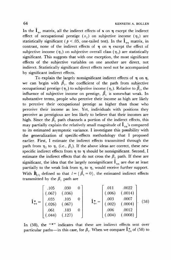
may partially explain the relatively small magnitude of I 's compared to its estimated asymptotic variance. I investigate this possibility with the generalization of specific-effects methodology that I proposed earlier. First, I estimate the indirect effects transmitted through the

path from r/2 to m/1 (i.e., 1P). If the above ideas are correct, these new

specific indirect effects from 1 to i1 should be nonsignificant. Second, I estimate the indirect effects that do not cross the /, path. If these are

significant, the idea that the largely nonsignificant IT, are due at least

partially to the weak link from T2 to r1i would receive further support. With B(/) defined so that l= { / = 0}, the estimated indirect effects transmitted by the P, path are

.105 .030 0 .011 .0022

(.067) (.036) (.006) (.0014) . 035 .105 0 ^ .003 .0007

(.026) (.067) nx (.002) (.0004) (8)

.061 .183 0 .006 .0012

(.044) (.127) (.004) (.0008)

In (58), the "*" indicates that these are indirect effects sent over

particular paths-in this case, for I,. When we compare I* of (58) to ? ~~~~~~T/r


I1, of (57), we see that all the indirect effects of T1 on Tq except the indirect effects of subjective income (q1,) on subjective overall class ('q3) are transmitted through the P, path. The indirect effect of 71T on 73 passed through the P, path is not statistically significant, although as shown in (57), the total indirect effect of m on i3 is statistically significant.

The indirect effects of x on q through the /,l path are even more

revealing. As I* shows, the only indirect effects through the ll path that are statistically significant are the effect of income (xl) on subjective income (q71) and the effect of occupational prestige (x2) on its subjective counterpart (q2). The remaining indirect effects of income and occupational prestige via the P, path are not significant. When I *

A 7x

is contrasted with I,X in (57), the secondary role that the influence of

subjective occupational prestige on subjective income plays in gener- ating total indirect effects of x on T is highlighted.

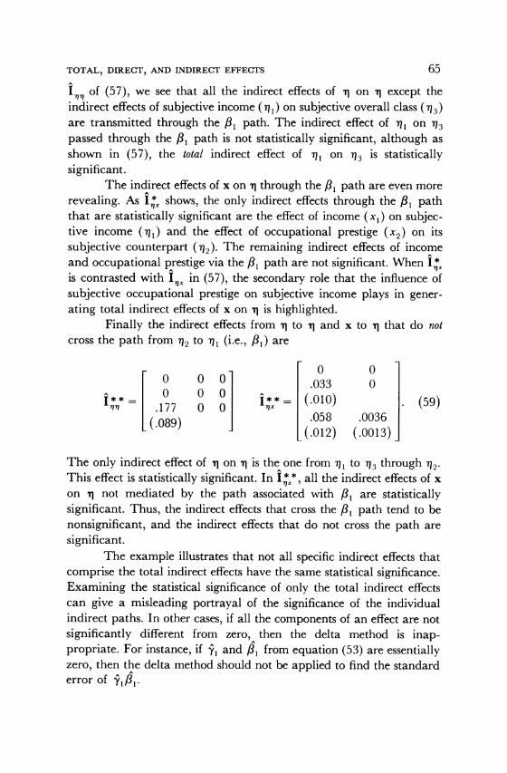
Finally the indirect effects from T to T and x to 1 that do not cross the path from q2 to m, (i.e., fl) are

0 0 0 0 0 .033 0

I - .7 0 0 I* (.010) . (59) A^7 .177 0 0 x

(.089) .058 .0036 (-.09 (.012) (.0013)

The only indirect effect of T on T is the one from m71 to 73 through iq2. This effect is statistically significant. In ,* , all the indirect effects of x on T not mediated by the path associated with fl are statistically significant. Thus, the indirect effects that cross the ,l path tend to be nonsignificant, and the indirect effects that do not cross the path are significant.

The example illustrates that not all specific indirect effects that comprise the total indirect effects have the same statistical significance. Examining the statistical significance of only the total indirect effects can give a misleading portrayal of the significance of the individual indirect paths. In other cases, if all the components of an effect are not significantly different from zero, then the delta method is inap- propriate. For instance, if Y, and P, from equation (53) are essentially zero, then the delta method should not be applied to find the standard error of 'Yl 1.

65

A final point bears repeating. The delta method is designed for

large-sample problems. The accuracy of the method for small samples is not known.

SUMMARY

Path analysis decomposition techniques have developed on a number of fronts, and the results are dispersed throughout the social science literature. In this paper, I have attempted to consolidate some of these findings. Drawing on earlier literature, I derived the total, indirect, and direct effects for the general LISREL model. I showed that to estimate total effects, whether defined as an infinite sum or as reduced-form coefficients, the convergence condition must be met. I reviewed the existing techniques for determining specific indirect effects, and I proposed a new procedure to estimate all types of specific effects. More generally, this procedure allows the researcher to trace the influence of any path or combination of paths in a model. Finally, using results from Folmer (1981) and Sobel (1982, 1986), I presented the standard errors for the various decompositions.

APPENDIX

To utilize the delta method for computing the asymptotic variance of the indirect effects, we must use the df(O)/d0. To simplify the results for the indirect effects, I define 0 to include only those unrestricted elements in B, r, and Ay. Each indirect effect is treated

separately. Sobel (1986, pp. 170-72) lists the partial derivatives for the indirect effects as

d vec I(A

do 1

= V( (I-B) r ((I-B)-1)) I) do V (A2)

d veclr I~

ado A) \ /(A3)

+Vr( ? ((I- -B) - I)')

' - Vy(((I- B)-- I) ?

Ip| (A3)

+V((I- B)-' ?(Ay(I-B)-')')


TOTAL, DIRECT, AND INDIRECT EFFECTS 67

dey = VB((I-B)-lr (A^y(I-B)-l)')

+VIr(I (AY(I-B)- )') (A4)

+V%((I-B) 11?Ir )

where

[ B dB aB1 VB = vecl , vec d vec-

a[ r ar Vr = vec --, vec ,...,vec -

[ A d02 dos VA = vec vec ... vec - A [ dO, 80, 0 9 O

vec = vec operator,

? = Kronecker's product.

For the empirical illustration in Figure 4, 0 = [f /i2 /,3 /34 ,1 y2]'. The VB and Vr matrices for I, and I1x are

O O O O O O 0 1 0 0 0 0 O 0 1 0 0 0 1 0 0 0 0 0

VB= o o o o o o (A5) O O 0 1 0 0 O O O O O O O O O O O O

,0 0 0 0 0 0

and

O O O 0 1 0 0 0 0 0 0 0(A 0 0 0 00 0 0 0 0 0 0 0 (A6) 0 0 0 0 0 1

_0 0 0 0 0 0

These are used to estimate the standard errors for I and Ix. The standard errors of the specific effects were estimated with appropriate modifications.


REFERENCES

ALWIN, DUANE F., AND ROBERT M. HAUSER. 1975. "The Decomposition of Effects in Path Analysis." American Sociological Review 40:37-47.

BEN-ISRAEL, A., AND T. N. E. GREVILLE. 1974. Generalized Inverses: Theory and

Applications. New York: Wiley.

BENTLER, PETER M., AND EDWARD H. FREEMAN. 1983. "Tests for Stability in Linear Structural Equation Systems." Psychometrika 48:143-45.

BISHOP, YVONNE M. M., STEPHEN E. FIENBERG, AND PAUL W. HOLLAND. 1975. Discrete Multivariate Analysis: Theory and Practice. Cambridge, MA: MIT Press.

BROWNE, M. W. 1984. "Asymptotic Distribution Free Methods in the Analysis of Covariance Structures." British Journal of Mathematical and Statistical Psychology 37:62-83.

DUNCAN, OTIS D. 1966. "Path Analysis: Sociological Examples." American Journal of Sociology 72:1-16.

.1975. Introduction to Structural Equation Models. New York: Academic Press.

FINNEY, J. M. 1972. "Indirect Effects in Path Analysis." Sociological Methods and Research 1:175-86.

FISHER, FRANKLIN M. 1970. "A Correspondence Principle for Simultaneous Equa- tion Models." Econometrica 38:73-92.

FOLMER, H. 1981. "Measurement of the Effects of Regional Policy Instruments by Means of Linear Structural Equation Models and Panel Data." Environment and

Planning 13:1435-48.

FOX, JOHN. 1980. "Effects Analysis in Structural Equation Models." Sociological Methods and Research 9:3-28.

1985. "Effects Analysis in Structural Equation Models II: Calculation of Specific Indirect Effects." Sociological Methods and Research 14:81-95.

FREEMAN, EDWARD H. 1982. "The Implementation of Effect Decomposition Meth- ods for Two General Structural Covariance Modeling Systems." Ph.D. diss., University of California at Los Angeles.

GOLDBERG, S. 1958. Introduction to Diference Equations. New York: Wiley.

GRAFF, j., AND P. SCHMIDT. 1982. "A General Model for Decomposition of Effects."

Pp. 131-48 in System Under Indirect Observation: Causality, Structure, and Prediction, edited by Karl G. Joreskog and Herman Wold. Amsterdam: North-Holland.

GREENE, VERNON L. 1977. "An Algorithm for Total and Indirect Causal Effects." Political Methodology 44:369-81.

JORESKOG, KARL G. 1978. "Structural Analysis of Covariance and Correlation Matrices." Psychometrika 43:443-77.

JORESKOG, KARL G., AND ARTHUR S. GOLDBERGER. 1975. "Estimation of a Model with

Multiple Indicators and Multiple Causes of a Single Latent Variable." Journal of the American Statistical Association 70:631-39.


JORESKOG, KARL G., AND DAG SORBOM. 1981. LISREL. Analysis of Linear Structural

Relationships by the Method of Maximum Likelihood. Version V. User's Guide. Chicago: National Educational Resources.

.1982. "Recent Developments in Structural Equation Modeling." Journal of Marketing Research 19:404-16.

KLUEGAL, JAMES R., ROYCE SINGLETON, JR., AND CHARLES E. STARNES. 1977. "Subjec- tive Class Identification: A Multiple Indicators Approach." American Sociological Review 42:599-611.

LUENBERGER, DAVID G. 1979. Introduction to Dynamic Systems. New York: Wiley. RAO, C. R. 1973. Linear Statistical Inference and its Applications. New York: Wiley.

SCHMIDT, PETER. 1978. "Decomposition of Effects in Causal Models." Revised version. Paper presented at the annual meetings of the Psychometric Society, Uppsala, Sweden.

SEARLE, SHAYLE R. 1982. Matrix Algebra Useful for Statistics. New York: Wiley.

SOBEL, MICHAEL. 1982. "Asymptotic Confidence Intervals for Indirect Effects in Structural Equation Models." Pp. 290-312 in Sociological Methodology 1982, edited by Samuel Leinhardt. San Francisco: Jossey-Bass.

.1986. "Some New Results on Indirect Effects and their Stan- dard Errors in Covariance Structure Models." Pp. 159-86 in Sociological Method- ology 1986, edited by Nancy B. Tuma. Washington, DC: American Sociological Association.

WILEY, DAVID E. 1973. "The Identification Problem for Structural Equation Models with Unmeasured Variables." Pp. 69-83 in Structural Equation Models in the Social Sciences, edited by Arthur S. Goldberger and Otis D. Duncan. New York: Seminar Press.

69

Date post:	11-Feb-2022
Category:	Documents
Upload:	others
View:	9 times
Download:	0 times

TOTAL, DIRECT, AND INDIRECT EFFECTS IN STRUCTURAL

Documents