Total Internal Reflection Fluorescence Cross-Correlation ... · Total Internal Reflection...

Total Internal Reflection Fluorescence

Cross-Correlation Spectroscopy: theory and

application for studying boundary slip

phenomenon

Dissertation zur Erlangung des Grades

“Doktor der Naturwissenschaften”

(Dr. rer. nat.)

im Promotionsfach Physik

am Fachbereich Physik, Mathematik und Informatik

der Johannes Gutenberg-Universität Mainz

vorgelegt von

Herrn Mast.-Phys. Stoyan Yordanov

geboren in Krumovgrad, Bulgaria

Mainz, 2011

ii

iii

Die vorliegende Arbeit wurde im Zeitraum von Oktober 2007 bis Juli 2011 am Max-Planck-

Institut für Polymerforschung in Mainz angefertigt.

Abgabedatum: 21.07.2011

Dekan:

Erster Berichterstatter:

Zweiter Berichterstatter:

Tag der mündlichen Prüfung: 30.09.2011

Angabe D77 Mainzer Dissertation

iv

v

Contents

Abstract 1

1. Introduction and Motivation 4

2. Overview of Fluorescence Correlation Spectroscopy (FCS) Technique 8

2.1. Conventional Fluorescence Correlation Spectroscopy 8

2.1.1. History of FCS 8

2.1.2. Experimental realization 9

2.1.3. Theory and data analysis 10

2.1.4. Limitation of the confocal FCS 19

2.2. Total Internal Reflection FCS (TIR-FCS) 20

2.2.1. Basic principles and concept 21

2.2.2. Experimental realization 27

2.2.3. Theory and data analysis 29

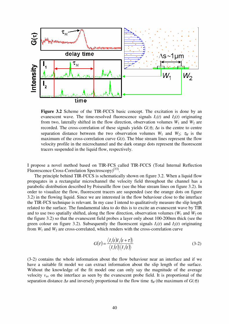
3. Total Internal Reflection Fluorescence Cross-Correlation Spectroscopy (TIR-FCCS)

– a novel approach to study flow near to an interface 39 3.1. Introduction to TIR-FCCS 39

3.2. Setup description 41

3.3. Analysis and simulations 43

3.3.1. Correlation functions 44

3.3.2. Algorithm description 47

3.3.3. Parameter space and dimensionless units 49

3.3.4. Numerical test – comparison of simulation with analytic solution 50

3.3.5. Statistical data analysis 51

3.3.5.1. Comparison of experiment and simulation 51

3.3.5.2. Determining good parameters and their statistical errors 53

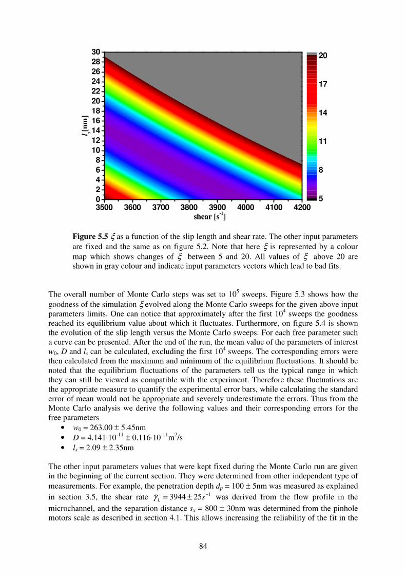
3.4. Estimation of the slip length accuracy 55

3.5. Penetration depth determination 61

4. Methods and Materials 65

4.1. TIR-FCCS equipment 65

4.2. Microchannel fabrication 70

4.3. Glass surface preparation 71

4.3.1. Hydrophilic surface 71

4.3.2. Hydrophobic surface 72

4.4. Fluorescence tracers 74

vi

5. Results and Discussion 78

5.1. Flow close to the interface and the slip problem 78

5.2. Flow on hydrophilic surface 80

5.3. Flow on hydrophobic surface 86

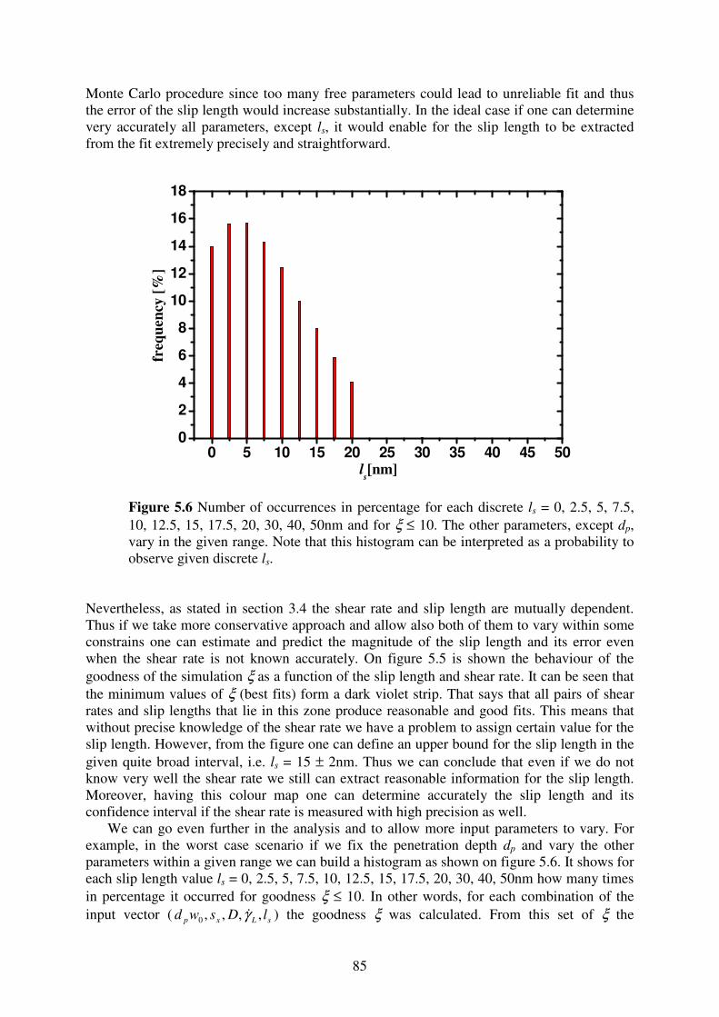
5.4. Discussion 93

Summary and Conclusion 100

A. Appendix 105

A.1. Approximation of Poiseuille flow with a linear function 105

A.2. Poiseuille flow with slip and non-slip boundary condition 108

List of symbols 117

List of abbreviations 120

References 121

Acknowledgements 129

Curriculum vitae 131

vii

Zusammenfassung

Im Rahmen dieser Arbeit wird die neue experimentelle Technik der Totalen Internen Reflexions Fluoreszenz-Kreuz-Korrelations-Spektroskopie (TIR-FKKS) vorgestellt. Mit dieser Methode können hydrodynamische Strömungen in Längenskalen von bis zu einigen 10-nm zu Festkörperoberflächen untersucht werden. Fluoreszierende Farbstoffe strömen mit der Flüssigkeit und werden mit evaneszentem Licht, welches mit Hilfe eines konfokalen Mikroskops und einem Öl-Immersions Objektiv mit einer hohen numerischen Apertur erzeugt wird, angeregt. Auf Grund des schnellen Abklingens der evaneszenten Welle tritt Fluoreszenz nur in unmittelbarer Nähe von etwa 100 nm zur Oberfläche auf, was eine sehr hohe Auflösung zur Folge hat. Die zeitaufgelösten Fluoreszenzsignale von zwei in Strömugsrichtung lateral verschobenen Detektionsvolumina, welche durch zwei konfokale Lochblenden erzeugt werden, werden unabhängig voneinander gemessen und aufgezeichnet. Die Kreuz-Korrelation dieser Signale liefert wichtige Informationen über die Bewegung der Farbstoffe und daher ihrer Strömungsgeschwindigkeit. Auf Grund der hohen Sensitivität der Methode können fluoreszierende Sorten von Farbstoffen, bis hin zu einzelnen Farbstoffmolekülen verwendet werden. Das Ziel dieser Arbeit war es den experimentellen Aufbau für TIR-FKKS zu konstruieren und damit die Scher-Rate und das Abgleiten von strömendem Wasser an hydrophilen, als auch hydrophoben Oberflächen zu messen. Um diese Informationen aus den gemessenen Korrelationskurven zu erhalten ist eine quantitative Datenanalyse notwendig. Dies ist nicht unkomliziert, wegen der Komplexität des Problems, die dass Ableiten einer analytische Lösung zur Bescheibung der Korrelationsfunktionen unmöglich macht. Um die experimentellen Daten zu bearbeiten und zu interpretieren, wird im Rahmen dieser Arbeit auch eine neue numerische Methode der Datenanalyse der erhaltenen Auto- und Kreuz-Korrelationskurven vorgestellt. Simulation von Brownschen Dynamiken werden benutzt um simulierte Auto- und Kreuzkorrelationsfunktionen zu erzeugen und die dazugehörigen experimentellen Daten zu beschreiben. Ich zeige wie detailierte und realistische theoretische Modelle des Phänomens mit genauen Messungen der Korrelationskurven kombiniert werden müssen um eine vollständig quantitative Methode zu entwickeln um die Ströumgeigenschaften aus dem Experiment abzuleiten. Eine Monte Carlo Simulation wird angewendet um die Exprimente zu beschreiben. Diese liefert die optimalen Parameterwerte und den statistischen Fehler. Diese Anwendung is sowohl geeignet für moderne Desktop PC‘s, als auch für parallel geschaltete Supercomputer. Der Letzere ermöglicht die Datenanalyse innerhalb kurzer Rechenzeiten. Ich habe diese Methode angewendet um die Strömungen von wässirigen Elektrolytlösungen in der Nähe von glatten hydrophilen und hydrophoben Oberflächen zu untersuchen. Im Allgemeinen wird an hydrophilen Oberflächen kein Abgleiten erwartet, während an hydrophoben Oberflächen Abgleiten auftreten kann. Unsere Ergebnisse zeigen, dass die Längen des Abgleitens etwa 10-15 nm oder geringer sind, sowohl auf hydrophilen als auch auf moderat hydrophoben (Kontaktwinkel etwa 85°) Oberflächen und damit im Rahmen der Fehler der Experimente nicht unterscheidbar von null.

2

Abstract I present a new experimental method called Total Internal Reflection Fluorescence Cross-Correlation Spectroscopy (TIR-FCCS). It is a method that can probe hydrodynamic flows near solid surfaces, on length scales of tens of nanometres. Fluorescent tracers flowing with the liquid are excited by evanescent light, produced by epi-illumination through the periphery of a high NA oil-immersion objective. Due to the fast decay of the evanescent wave, fluorescence only occurs for tracers in the ~100 nm proximity of the surface, thus resulting in very high normal resolution. The time-resolved fluorescence intensity signals from two laterally shifted (in flow direction) observation volumes, created by two confocal pinholes are independently measured and recorded. The cross-correlation of these signals provides important information for the tracers’ motion and thus their flow velocity. Due to the high sensitivity of the method, fluorescent species with different size, down to single dye molecules can be used as tracers. The aim of my work was to build an experimental setup for TIR-FCCS and use it to experimentally measure the shear rate and slip length of water flowing on hydrophilic and hydrophobic surfaces. However, in order to extract these parameters from the measured correlation curves a quantitative data analysis is needed. This is not straightforward task due to the complexity of the problem, which makes the derivation of analytical expressions for the correlation functions needed to fit the experimental data, impossible. Therefore in order to process and interpret the experimental results I also describe a new numerical method of data analysis of the acquired auto- and cross-correlation curves – Brownian Dynamics techniques are used to produce simulated auto- and cross-correlation functions and to fit the corresponding experimental data. I show how to combine detailed and fairly realistic theoretical modelling of the phenomena with accurate measurements of the correlation functions, in order to establish a fully quantitative method to retrieve the flow properties from the experiments. An importance-sampling Monte Carlo procedure is employed in order to fit the experiments. This provides the optimum parameter values together with their statistical error bars. The approach is well suited for both modern desktop PC machines and massively parallel computers. The latter allows making the data analysis within short computing times. I applied this method to study flow of aqueous electrolyte solution near smooth hydrophilic and hydrophobic surfaces. Generally on hydrophilic surface slip is not expected, while on hydrophobic surface some slippage may exists. Our results show that on both hydrophilic and moderately hydrophobic (contact angle ~85°) surfaces the slip length is ~10-15nm or lower, and within the limitations of the experiments and the model, indistinguishable from zero.

3

4

1. Introduction and Motivation A good understanding of the liquid flow in confined geometries is not only of fundamental interest but is also very important for a number of industrial and technological processes, such as flow in porous media, electro-osmotic flow, particle aggregation or sedimentation, extrusion and lubrication. It is also essential for the design of micro- and nano-fluidic devices, e.g. in a lab-on-chip applications. In all these cases, however, an accurate quantitative description can be done only if the flow at the interface between the fluid and the solid is thoroughly understood[1],[2],[3],[4],[5],[6],[7],[8],[9],[10]. While for many years the so called no-slip boundary condition (velocity equals to zero on the interface) was applied to describe macroscopic flows, recently it has been recognized that this condition does not always apply when flows through channels with micro- and nano-sizes are considered[4],[5]. In such channels the fluid may slip over the solid surface. This effect is usually described by the so called slip boundary condition, characterized by a non vanishing slip length ls which is defined as the ratio of the dynamic viscosity and the friction coefficient of the liquid at the surface, or equivalently as the ratio of the finite flow velocity at the surface, so called slip velocity vs, and the shear rate at the surface

( )0=

∂∂=

z

ss

zv

vl

where z is the spatial direction, perpendicular to the surface. Experimental approaches allowing determination of this slip length, however, are very challenging, since very high resolution techniques are needed to gain any information close to the interface. Hence, the existence and the extent of a slip in real physical systems as well as its possible dependence on the surface properties are highly debated in the community and no consensus has been reached so far. Clearly, to rationalize this controversy, further refinement of the experimental techniques is required. To date, two major types of experimental methods, often called direct and indirect, were applied to study boundary slip phenomena. In the indirect approach, an atomic force microscope or a surface force apparatus, is used to record the hydrodynamic drainage force necessary to push a micron-sized colloidal particle versus a flat surface as a function of their separation[11],[12]. The separation can be measured with sub-nanometre resolution, and the force with a resolution in the pN range. A higher force is necessary to squeeze the liquid out of the gap if the mobility of the liquid is small. Instead, if the liquid close to the surface can easily slip on it, then a smaller force is necessary. From this empirical observation a quantitative value of the slip length can be deduced using an appropriate theoretical model[2]

,[6],[13]. While this approach is extremely accurate at the nanoscale, it does not measure directly the flow profile and rely on a theoretical modelling. Direct experimental approaches to flow profiling in microchannels, are commonly based on various optical methods to monitor fluorescent tracers flowing with the liquid. Basically they can be divided in two sub categories. The imaging based methods use high resolution optical microscopes and sensitive cameras to track the movement of individual tracer particles on a series of images[14],[15],[16],[17],[18],[19],[20]. While providing a real “picture” of the flow, the imaging methods have also some disadvantages related mainly to the limited speed and sensitivity of the cameras: relatively big tracers are needed, the statistic is rather poor, high tracer velocities cannot be easily measured.

5

In Fluorescence Correlation Spectroscopy (FCS) based methods the fluctuations of the fluorescent light emitted by tracers passing through a very small observation volume (typically the focus of a confocal microscope) is measured[21]. Using correlation analysis and an appropriate mathematical model the tracers’ diffusion coefficient and flow velocity can be evaluated[22],[23],[24],[25]. In particular, the so called double-focus fluorescence cross-correlation spectroscopy (DF-FCS) that employs two observation volumes (laterally shifted in flow direction) is a very powerful tool for flow profiling in microchannels[26],[27],[28],[29]. Due to the very high sensitivity and speed of the used photo detectors (typically avalanche photodiodes) in FCS based methods even single molecules can be used as tracers. Furthermore, the evaluation of the velocity is based on large statistics and high tracer velocities can be measured. During the last two decades both the imaging and the FCS methods were well developed to the current state that allows fast and accurate measurements of flow velocity profiles in microchannels. The situation, however, is different when the issue of boundary slip is considered. Due to the limited optical resolution imposed by the diffraction limit, it is commonly considered that these methods are less accurate than the force methods discussed above and cannot detect a slip length in the tens of nanometres range. On the other hand the possibility to directly visualize the flow makes the optical methods still very attractive and thus continuous efforts were undertaken to improve their resolution. One of the most successful approaches in this endeavour is Total Internal Reflection Microscopy (TIRM)[30]. In TIRM the effect of total internal reflection on the interface between two media with different refractive indices (e.g. glass and water) is used to create an evanescent wave that extends (and therefore can excite the fluorescent tracers) only in a tunable region of less than 200nm from the interface. During the last few years TIRM was successfully applied for improving the normal resolution of the particle imaging velocimetry close to solid interfaces[17],[18],[19],[20] and slip lengths in the order of tens of nanometres were evaluated. With respect to FCS, however, TIR illumination was limited to diffusion studies only[31],[32] and there are no reports for TIR-FCS based velocimetry and slip length measurements. Therefore, the main aim of this thesis is to propose a new experimental setup that combines for the first time TIR illumination with double-focus fluorescence cross-correlation spectroscopy for monitoring a liquid flow in the very close proximity of a solid surface[33]. Such combination offers very high normal resolution, extreme sensitivity (down to single molecules), very good statistic obtained for relatively short measurement times and the possibility to study very fast flows. Our initial studies have shown, however, that the accurate quantitative evaluation of the experimental data obtained with this TIR-FCCS setup is not straightforward because the model functions needed to fit the measured auto- and cross-correlation curves (and extract the flow velocity profile) are not readily available. The standard analytical procedure to derive these functions is[26],[27],[28]:

1. Solve the diffusion-convection equation with respect to the concentration correlation function (see eq. (3-11))

2. Insert the derived solution in the corresponding correlation integral (see eq. (3-8)) 3. Solve it to finally get the explicit form of the correlation functions

This procedure was successfully used by Brinkmeier et al [26] to derive analytical expressions for the auto- and cross-correlation functions obtained with double focus confocal FCCS (i.e. with focused laser beam illumination as opposed to the evanescent wave illumination in my case) assuming that the local flow velocity and tracers concentration do not depend on the normal coordinate z, i.e. an average velocity can be used for all tracers inside the observation volume. Such an assumption is reasonable only if the observation volumes (laser foci) are far away from the channel walls. In the case of TIR-FCCS, however,

6

the situation is different as the experiments are performed in the very proximity of the channel wall and the distribution of the flow velocity inside the observation volume has to be considered. Furthermore, the concentration of tracers may also depend on z due to the electrostatic repulsion or hydrodynamic effects. Finally the presence of a boundary, which must be also taken into account in the theoretical treatment, further complicates the problem. All this effects would likely render the convection-diffusion equation (CDE) unsolvable in the case of TIR-FCCS. But even if an analytical solution of CDE can be found it would be complicated and the solution of the correlation integral hardly achieved. Therefore as an alternative of the above described analytical approach in this thesis I also describe a novel numerical method for quantitative data analysis of TIR-FCCS correlation curves in the presence of an external flow. I employ Brownian-Dynamics techniques to simulate the tracers’ motion through the observation volumes and generate “numerical” auto- and cross-correlation curves that are consequently used to fit the corresponding experimental data. Moreover, a Monte Carlo method is employed for a systematic data analysis. This numerical approach overcomes all the problems posed to the analytical solution by the complicated experimental geometry. Furthermore, it has the potential to easily include effects such as hydrodynamic slow down of tracers’ diffusion and their electrostatic interaction with the channel wall as well as to account for different geometry of the observation volumes. I used, in particular, the newly developed TIR-FCCS experimental setup and the numerical data evaluation procedure to study aqueous flow near a smooth hydrophilic surface and evaluated the slip length to be between 0 and 10nm. As it is commonly accepted[16],[18],[19],[20],[34],[35],[36] that the boundary slip should be zero in the situation of hydrophilic surface, my results indicate that the TIR-FCCS offers an unprecedented for an optical method accuracy in the nanometre range – down to few nanometres. The structure of the thesis is organized as follows: Chapter 2 is dedicated to the basic theory and concept of Fluorescence Correlation Spectroscopy (FCS). It gives a short overview of the technique, its applications and experimental realization. Furthermore, the fundamentals of so called Total Internal Reflection Fluorescence Correlation Spectroscopy (TIR-FCS) are described. This technique is the base of the proposed in the thesis TIR-FCCS method. Therefore, it is important for the understanding of the remaining of the thesis. Chapter 3 explains the principles, the concept and the setup of the newly proposed TIR-FCCS technique. Likewise, it presents a numerical model that employs Brownian Dynamics in order to quantitatively process the experimental data; the limitations and the accuracy of the technique are also analyzed. Chapter 4 contains technical information about the materials and equipment that were used in the study – equipment description, microchannel fabrication, hydrophilic/hydrophobic surface preparation, as well as discussion on the fluorescence tracers. Finally Chapter 5 presents the experimental results obtain with TIR-FCCS technique. A detail analysis and discussion about the measured slip on hydrophilic and hydrophobic surfaces is also presented. The boundary-slip issue and the physical origin of the slip are also discussed.

7

8

2. Overview of Fluorescence Correlation Spectroscopy (FCS) Technique

2.1. Conventional Fluorescence Correlation Spectroscopy Fluorescence Correlation Spectroscopy (FCS) is a highly spatial and time resolution technique which uses the fluctuations in the light intensity signal to analyze the dynamic properties and behaviour of fluorescent or fluorescently labelled single molecules, macromolecules, nanoparticles etc. in solution. The fluctuations in the light intensity are typically due to the statistical nature of the undergoing process such as Brownian motion, thermal noise, a chemical reaction and so on. Generally any physical parameter that causes intensity fluctuations can be monitored and hence studied by FCS. For example, FCS is widely used to study the diffusion of fluorescent species in a system. When an appropriate physical model of the fluctuations is known, quantitative information for the following physical parameters can be extracted:

• diffusion coefficient • hydrodynamic radius • average concentration

A sensitive detector records the fluctuation in the intensity emitted by fluorescent markers. It results in intensity vs. time trace representing random noise. From this data a correlation function is generated and the following information extracted - diffusion time, respectively the hydrodynamic radius, and the number of molecules, equivalent to the concentration in the sample. Besides the Brownian motion, as mentioned above, FCS can analyze other sources of fluorescence fluctuations, including electronic properties of dyes (e.g. triplet states), hindered diffusion, active transport and changes in FRET signals due to conformational changes of molecules. When only one kind of fluorescent marker and one detector are used, the method is named auto-correlation. In order to distinguish between two different types of molecules or a small molecule bound to a big one a difference of mass of at least 1.4 is required. Thus to increase the sensitivity of the method, two markers and detectors can be used. This method is called cross-correlation. Other common methods to use fluorescence fluctuations to probe molecular interactions include Photon Counting Histograms (PCH) and Fluorescence Intensity Distribution Analysis (FIDA). Coincidence Analysis is used to probe rare events in the femto-molar range.

2.1.1. History of FCS FCS was introduced for first time in the early 1970s in a series of publications[37],[38],[39] by Madge, Elson and Webb. In these papers they present the basic concept and theory of FCS as well as its potential to measure the chemical rate constants and diffusion coefficients of fluorescently labelled molecules. For example, they reported data for binding of ethidium bromide (a fluorescent tag) to DNA. Later on in 1978 they published a paper[22] that described the abilities of FCS to measure uniform translation or laminar flow in a sample cell. However, in the early times of FCS era the measurements suffered from low signal-to-noise ratios due

9

to the high number of observed molecules, intensity instability in the laser light sources, low quantum yield fluorophores and low detector efficiency. Unlike the pure fluorescence intensity measurements, where a solution with high fluorophores concentration is needed, FCS measurements are best realized when the average number of fluorescent tracers in the observation volume does not exceed 5-10. Typical concentrations of fluorophores in the nowadays FCS experiments are in the nanomolar range. Since all these requirements and drawbacks FCS was not widely used for 20 years. However, in the early 1990s number of technical improvements helped to refine the FCS technique. The major improvement was achieved by Rigler and his co-workers[40] (in 1993) by introducing of so called confocal detection scheme (for details see the next section), which helped to decrease significantly the observation volume and increase dramatically the S/N (signal-to-noise ratio). Subsequently the improvement of the laser source stability as well as the detection efficiency by using of avalanche photodiodes (APD) and high numerical aperture microscope objectives led to even single photon sensitivity. This extended the range of application of FCS to conformational changes in biomolecules and photo dynamical properties of fluorescent dyes. Other prominent applications of FCS are to investigate protein association reactions, DNA hybridization, immunoassays, binding to membrane receptors, gene expression, diffusion in hydrogels, diffusion in polymer melts, microflows and so on. In all these cases FCS offers extremely high selectivity and sensitivity (down to single molecule level) combined with very small probing volume of less than 1µm3.

2.1.2. Experimental realization A scheme of typical FCS setup is shown on figure 2.1. It consists of a light source, usually laser which is fibre coupled to a microscope, dichroic mirror, emission filter, adjustable pinhole, and detection unit (usually APD or photo multiplayer). The excitation laser beam (blue on the figure 2.1) is expanded and collimated in order to fill in the objective aperture, then it is reflected by the dichroic mirror and focused by a high numerical aperture (typically NA>1) objective to a diffraction limited spot (<0.5µm) in the sample space. The fluorescent light (the green on figure 2.1) originating from the focus is collected back by the same microscope objective, passes through the dichroic mirror, emission filter and confocal pinhole and is finally recorded by a detector, typically an avalanche photodiode (APD). The recorded signal is correlated by software or hardware correlator and a correlation curve is produced. In most cases the correlation curve is monitored on a computer screen in real time during the measurement, which allows better control and adjustment of the system. The data usually can be stored in ASCII format for easy processing and analyzing later with the available mathematical software. The wavelength of the laser is chosen in such a way that the fluorophores can be excited efficiently, respectively, the dichroic mirror, which is kind of wavelength beam splitter must be transparent for the fluorescence and to reflect the excitation light. Also the emission filter must stop completely the scattered excitation light and to be transparent for the fluorescence emission. On the other hand the role of the pinhole is to cut-off the light coming out of the focus, which in turn significantly increases both the S/N and the axial as well as lateral resolution of the system. Thus the typical confocal observation volume of the FCS system is as small as 1µm3 (≤1fL). This allows measurements to be performed with high spatial resolution and in small samples, e.g. even in living cells.

10

Figure 2.1 Scheme of a typical FCS setup. The magnified image on the right shows zoom in view of the confocal volume (green) and the excitation envelope (cyan) in the objective’s focus.

2.1.3. Theory and data analysis In order to extract quantitative information about a system under investigation we need an appropriate model that describes the correlation function observed in an FCS experiment. Since there are broad ranges of systems, and the equations that govern the underlying physical processes can be quite complex, here I describe only the fundamental cases of translational free three-dimensional diffusion and directed flow, which are important for understanding of my study. In the most general case the auto-correlation function of the intensity fluctuations (see figure 2.2) is given by the mean of the following product[38],[39],[41]

( ) ( ) ( ) ( ) ( )∫ +=+=T

dttItIT

tItIg0

1τττ (2-1)

where I(t) is the time dependent fluorescence intensity due to the fluorescent molecules, τ is the delay time, and T is the measurement time. In practice the more convenient form of a normalized auto-correlation function by the squared intensity is used

11

( ) ( )( ) ( )

( ) ( )( ) ( )

( ) ( )2

01

I

II

tItI

tItI

tItI

gG

τδδτττ +=

+== (2-2)

Here in order to get equation (2-2) one uses the fact that the quantity of interest is the fluctuation in the light intensity δI(t)

( ) ( ) ( )tItItI −=δ , (2-3)

as well for ergodic systems

( ) 0=tIδ , (2-4)

and that delay time τ is always relative to an earlier moment, so only the difference τ makes sense, hence the substitution t = 0 is justified[41].

Figure 2.2 Fluorescence intensity fluctuations due to the particles’ Brownian motion. As one can see from the magnified fluorescence vs. time trace on figure 2.2, the fluctuations δI(t) in the fluorescent intensity are due to changes in the local concentration of the fluorescent species in the observation volume. Mathematically this is expressed with the following equation[41]

( ) ( ) ( )( )dVtrBCrWtIV

,rr

δδ ∫= (2-5a)

As well as the intensity I(t) is given by

12

( ) ( ) ( )( )dVtrBCrWtIV

,rr

∫= (2-5b)

where B is a parameter called molecular brightness, and it describes the properties of the fluorophores and the FCS system such as the quantum efficiency for detection of the emitted photons, quantum yield for emission of photons, and the cross-section for absorption. Usually within a FCS experiment this parameter is assumed to be a constant so that equation (2-5) can be rewritten as

( ) ( ) ( )dVtrCrWBtIV

,rr

δδ ∫= (2-6a)

and


,rr

∫= (2-6b)

( )rWr

is the so called molecular detection efficiency MDE function and describes the

excitation intensity distribution in the focal volume V and the collection efficiency of the objective plus detector system. In practice for small pinholes, in the order of or smaller than the Airy unit (AU) of the objective, this function can be very well approximated with three-dimensional Gaussian function[41],[21] with characteristic size in x-y plane r0 and axial size along z-axis z0 (see figure 2.3)

( )

−

+−=

20

2

20

22

0 2exp2expz

z

r

yxIrW

r (2-7)

I0 is the intensity amplitude. The last term in (2-6a), ( )τδ ,rC

r, refers to the local fluctuations in

the concentration ( )τ,rCr

due to the particles’ Brownian motion, i.e. ( ) ( )ττδ ,, rCCrCrr

−= .

Substituting (2-6) in (2-2) yields the integral representation of the normalized auto-correlation function

( )( ) ( ) ( ) ( )

( )2

2 ,0,

1

′′′

+=

∫

∫ ∫′

V

V V

dVrWBC

VdVdrCrCrWrWB

G

r

rrrrτδδ

τ (2-8)

We can simplify the latter expression by cancelling out the B term

( )( ) ( ) ( )

( )2

2

,,

1

′′′

+=

∫

∫ ∫′

V

V V

dVrWC

VdVdrrrWrW

G

r

rrrrτφ

τ (2-9)

and making a substitution according

13

Figure 2.3 Schematic drawing of the FCS observation volume and the excitation beam – r0 and z0 denote the lateral, respectively, axial size of the observation volume.

( ) ( ) ( )τδδτφ ,0,,, rCrCrrrrrr

′=′ (2-10)

The last step towards the integration of (2-9) is to find the explicit form of (2-10) which is called concentration correlation function and contains the dynamic behaviour of our system. This function represents the correlation between two particle’s positions in space and time, if at time t = 0 the particle is at ( )zyxr ′′′=′ ,,

r then it shows the probability to find the particle at

( )zyxr ,,=r

at time t = τ. C is the average concentration of the fluorescent particles. In

order to find ( )τφ ,, rr ′rr

we have to solve the equation that govern the dynamics of the system.

In the case of free three-dimensional diffusion it is the diffusion equation

( ) ( )τδτ

τδ,

,rCD

rC rr

∆=∂

∂ (2-11)

Multiplying this equation with ( )0,rC ′

rδ , and taking into account (2-10), gives an equation for

( )τφ ,, rr ′rr

( ) ( )τφ

ττφ

,,,,

rrDrr ′∆=

∂

′∂ rrrr

(2-12)

The latter equation can be solved by Fourier Transform and has a closed-form[38],[22],[41] solution, namely

14

10-6

10-5

10-4

10-3

10-2

10-1

100

1.0

1.1

1.2

1.3

1.4

1.5

Experimental data Fit yields: τ

D = 232µs, N = 2.12

G( ττ ττ

)

ττττ [s]

Figure 2.4 a) Example of an auto-correlation curve and its development; b) Example of a fit of an auto-correlation curve – solid red line is the fit with (2-19) and circles are the experimental points. Note that the tracers used were Qdots585 and S = 6 (fixed).

a)

b)

15

( )( )

′−−=′

ττπτφ

D

rr

D

Crr

4exp

4,,

2

2

3

rrrr

(2-13)

with initial condition at τ = 0

( ) ( )rrCrr ′−=′rrrr

δφ 0,, (2-14)

where D is the diffusion coefficient. Having in hands (2-13) and (2-7), and substituting them in (2-9), and doing some exhaustive mathematical calculations we finally get for G(τ)

( )( ) 2

02

02

3

44

11

zDrDC

G

++

+=

ττπτ (2-15)

If we rewrite the upper expression in the following form

( )20

20

02

02

34

14

1

11

z

D

r

DzrC

Gττ

πτ

+

+

+= (2-16)

and insert

D

rD

4

20=τ (2-17)

as well

0

0

r

zS = (2-18)

we get the widely used in practice, and more convenient in form, auto-correlation function[41]

( )

DD SN

G

ττ

ττ

τ

211

11

+

+

+= (2-19)

N is the average number of particles in the observation volume and is derived from

NVCzrC eff ==02

02

3

π , where 02

02

3

zrVeff π= has the dimension of volume and is called

effective volume; τD is the so called diffusion time – it can be thought as the average time that a particle needs to cross the observation volume; S is the so called structure parameter – the ratio between axial and lateral extent of the observation volume (see (2-18)). Equation (2-19) is important because it describes the observed experimental auto-correlation curve and is used in the data fitting analysis in order to extract the diffusion time τD and the number of particles N (see figure 2.4). Thus using (2-17) one can derive the

16

diffusion coefficient and through Einstein-Stokes equation, the hydrodynamic radius of the particle

D

kTRh πη6

= (2-20)

where Rh – hydrodynamic radius; k – Boltzmann’s constant; η - viscosity of the medium; T – temperature. In case when there is a directed flow presented, e.g. along x axis (see figure 2.5), we have to modify (2-11), (2-12) in such a way that to account for that. Therefore the concentration fluctuations ( )τδ ,rC

r and concentration correlation function ( )τφ ,, rr ′

rr, in case of flow, obey

to the following differential equations

( ) ( ) ( )

x

rCVrCD

rCx ∂

∂−∆=

∂∂ τδ

τδτ

τδ ,,

,r

rr

(2-21)

( ) ( ) ( )

x

rrVrrD

rrx ∂

′∂−′∆=

∂

′∂ τφτφ

ττφ ,,

,,,,

rrrr

rr

(2-22)

Vx denotes the flow velocity, which in our case of directed uniform flow is a constant. The solution of the latter differential equation is known[22],[24] and has the following form

( )( )

( ) ( ) ( )

′−+′−+−′−−=′

ττ

τπτφ

D

zzyyVxx

D

Crr x

4exp

4,,

222

2

3

rr (2-23)

Substituting this function in (2-9) and taking into account (2-10) and (2-14) one can derive the corresponding auto-correlation function in the flow case. It has similar form like (2-19), but additional exponential term appears that accounts for the presence of flow[22],[24]

( )

+

−

+

+

+=

D

f

DD SN

G

τττ

τ

ττ

ττ

τ1

1exp

11

11

2

2

(2-24)

where τf is the flow time, and is defined as follows

x

fV

r0=τ (2-25)

i.e. the average time that a particle needs to travel a distance equal to the radius of the observation volume.

17

Figure 2.5 Scheme of the FCS observation volume and directed flow along x axis. This closed-form view of the auto-correlation function (2-24) allows straightforward fitting of the experimental data and hence easy measurement of a flow profile throughout a micro channel, which is important part from the method I have developed. So far we have assumed that the observed intensity fluctuations were caused by the random walk of the fluorescent particles throughout the confocal FCS volume. However due to the physical nature of the particles they may change their intrinsic fluorescence properties during the observation. For instance, many fluorescence molecules such as Alexa488, Rh6G, green fluorescent protein etc. can be excited in triplet state (see figure 2.6).

a) b)

Figure 2.6 Scheme of light absorption that excites a fluorophore to singlet state S1 and the relaxation a) from singlet to ground state S1 S0, and b) relaxation from singlet to ground state through triplet state S1 T1 S0.

18

Fraction of the excited molecules relaxes to the ground state through the triplet state. This fact leads to additional raise in the auto-correlation curve caused by the triplet relaxation process which is observed at short times, usually about few microseconds[42] (see figure 2.7). In order to account for this process, and when we cannot avoid the triplet in our data analysis, the so called triplet correction term is added to the auto-correlation fit function[42],[43]

p

p

Trtr

−

−

+=1

exp

1ττ

(2-25)

where p is the percentage of molecules that has entered in triplet state, and τtr is the triplet decay time. Thus the corresponding auto-correlation reads

10-9

10-8

10-7

10-6

10-5

10-4

10-3

10-2

10-1

100

1.0

1.2

1.4

1.6

1.8

Antibunching

Rotational Diffusion

Triplet

Diffusion

Au

to-c

orre

lati

on

ττττ [s]

Figure 2.7 Time scale of different photo-physical processes observed by FCS

( )

DD

tr

SN

p

p

G

ττ

ττ

ττ

τ

211

1

1

exp

11

+

+

−

−

++= (2-26)

Note that for processes where the dynamics is not as fast as the triplet decay time, the triplet term can be neglected. There are other short time processes that can give raise in the auto-correlation curve and can be eventually monitored by FCS[21], e.g. rotational diffusion, antibunching etc. However in most cases of diffusion measurements these processes occur at very short time scales and can be neglected.

19

2.1.4. Limitation of the confocal FCS FCS has proved to be a versatile and powerful tool to study great number of phenomena ranging from biology and chemistry to physics. For example, due to the small observation volume (<1fL) FCS is widely used in biology in order to study intracellular interactions as well as transport of biomolecules in living cells. Moreover, this advantage of such a small confocal volume and its non-invasive capability allow in situ to probe various kind of interactions in living cells so that the mechanism of important biochemical and biophysical processes can be revealed. Even though the conventional FCS presented in the latter section has certain limitations inherited by the requirement to use optical wavelengths to create and record the fluorescence signal. Therefore due to the diffraction of the light with conventional means one cannot achieve lateral size of the observation volume smaller than the half of the wavelength of the light used[44]

objNA

r2

22.10

λ= (2-27)

Furthermore, in axial direction the resolution is even worse[44]

20

5.1

objNA

nz

λ= (2-28)

where λ – wavelength of the light, NAobj – numerical aperture of the objective, n – refractive index of the medium. The latter two expressions are derived taking into account the so called diffraction limit of the light and typically in the FCS case the corresponding values are about r0 ~250nm in lateral and z0 ~700nm in normal direction, respectively (as λ = 488nm, NAobj = 1.2, n = 1.33). As a direct consequence of this, number of important phenomena becomes inaccessible by the conventional FCS technique. Moreover, when one applies FCS to study surface phenomena quantitative results are either difficult to get or impossible. Thus when one investigates flow near a solid interface, and essentially so called boundary slip phenomenon, better axial resolution is required. In order to achieve it I used another technique called Total Internal Reflection Fluorescence Correlation Spectroscopy (TIR-FCS). TIR-FCS is further development of FCS technique, based on Total Internal Reflection effect that may be used to address the boundary slip issue. In next section I describe the basic concept and idea behind TIR-FCS, and why it can be useful to study processes that take place near an interface. As well as I present the theory of evanescent wave and data analysis approach in TIR-FCS. This is an important step towards the understanding of the next chapters where I describe my contribution by proposing Total Internal Reflection Fluorescence Cross-Correlation Spectroscopy (TIR-FCCS) in order to study the boundary slip phenomenon. So in summary the TIR-FCS aims to overcome the following basic problems that occur in conventional FCS technique:

• FCS observation volume is too big along the normal to the surface • FCS observation volumes is not well defined on the surface • The S/N is not as good as in TIR-FCS

20

2.2. Total Internal Reflection FCS (TIR-FCS) The effect of Total Internal Reflection takes place on the interface between two media with different refractive indices and result in the appearance of an evanescent (fast decaying) wave in the low refractive index media. The so called Total Internal Reflection Spectroscopy for optical absorption studies (called also attenuated total reflection or ATR) a has been developed in the early 60s and widely used in surface chemistry studies[45]. A book that describes in details this method is “Internal Reflection Spectroscopy” by Harrick[46]. As a technique for selective surface illumination in fluorescence studies, Total Internal Reflection Fluorescence (TIRF) was first introduced by Hirschfeld[47] for solid-liquid interfaces, Tweet et al.[48] for liquid-air interfaces, and Carniglia et al.[49] for high refractive index liquid-solid interfaces. TIRF has been combined with variety of other conventional fluorescence techniques (polarization, Fröster energy transfer, microscopy, spectral analysis, photo-bleaching recovery, and correlation spectroscopy) for a variety of reasons (detection of molecular adsorption, measurement of adsorption equilibrium constants, kinetic rates, surface diffusion etc.). Total Internal Reflection optics have also been combined with Raman spectroscopy[50],[51], infrared absorption spectroscopy[52], and light scattering[53],[54]. Total Internal Reflection Fluorescence Microscopy (TIRFM) is other prominent domain where TIR effect is applied[55]. Its aim is to visualize objects and events near a surface with higher axial resolution and as well as higher contrast. For example, a popular application is selectively to image structures in living cells, excite fluorophores close to the cover slip, and track surface dynamics of cell’s membrane[56]. For example, TIR generates rapidly decaying evanescent field near the surface so that a thin illuminated layer (~100nm) close to the interface is visualized, such as basal plasma membrane (~8nm thick) of living cells. The combination of TIRF with correlation spectroscopy led to TIR-FCS. It is an optical technique based on FCS, which is intended to study phenomena at solid-liquid interfaces. Similar to FCS, it uses the light fluctuations and correlation analysis in order to extract information about the dynamic properties of a system under investigation, such as a diffusion coefficient, concentration of the fluorescent species etc. It was introduced in the early 1980s by Thomson et al.[57],[58] who employed TIR effect to FCS in order to improve the S/N of the FCS technique. At that time the confocal principle was still unknown and this was useful approach to reduce the background noise in a FCS experiment. Likewise the axial resolution of FCS was increased, which allowed selective excitation of fluorescent samples in very proximity to the surface (~100nm). Such studies are important to a broad range of scientific and industrial processes – specific or non-specific binding to an interface, blood coagulation at foreign surfaces, diffusion in cell’s membrane etc. Although the fundamentals of TIR-FCS theory were established in the beginning of 1980s, the technique did not spread much in the next years. Increased number of publications that showed experimentally the application of the method to other fields in life science followed exclusively in the late 1990s. For example, Hansen et al.[59] investigated reversible adsorption kinetics of the cationic dye Rh6G to modified silica surfaces. TIR-FCS was also used to investigate molecular transport in thin sol-gel (porous silicon oxide) films[60].

21

2.2.1. Basic principles and concept a) b)

c)

As mentioned in the latter section TIR-FCS is technique developed to improve the axial resolution of the confocal FCS as well as to address the questions related to studies on the interface. Employing Total Internal Reflection (TIR) effect to FCS technique leads to higher axial resolution of the system. Thus the main difference between confocal-FCS and TIR-FCS technique is the way in which the excitation is realized. In TIR-FCS the excitation is done by evanescent field when Total Internal Reflection takes place. The phenomenon occurs on the border of two media with different refractive indexes when the light beam comes from higher refractive index medium to lower refractive index medium at angle of incident exceeding the so called critical angle (see figure 2.8). Then the so called evanescent field arises in the medium with lower refractive index n2 and excites the fluorophores only in proximity of the interface within a layer typically 60nm to 250nm thick. The axial extend of this layer (so called penetration depth dp) is governed by laser beam angle of incidence (see figure 2.9b) as well as the refractive indexes of the media. When a plain electromagnetic wave propagates and reaches the interface between two media it undergoes refraction described by Snell’s law

Figure 2.8 Scheme illustrating Total Internal Reflection effect and the excited evanescent field – a) α1 < αc – angle of incidence α1 bellow the critical angle αc; b) α1 = αc – angle of incidence α1 equal to the critical angle αc; c) α1 > αc – angle of incidence α1 above the critical angle αc - Total Internal Reflection occurs as well as evanescent wave arises in the medium with lower refractive index n2.

22

1

2

2

1

sin

sin

n

n=

αα

(2-29)

where α1 – angle of incidence, α2 – angle of refraction, n1 – refractive index of medium 1, n2 – refractive index of medium 2. In our case in order to achieve TIR we impose n2 < n1, i.e. the first medium is optically denser than the second medium – a requirement for Total Internal Reflection to be observed. Thus the critical angle αc, the smallest angle when TIR occurs, is defined as the angle of incidence α1 where the angle of refraction α2 becomes 90°, i.e. refracted beam propagates parallel to the interface (see also figure 2.8b)

=⇒=

°−

1

21

1

2 sin90sin

sin

n

n

n

nc

c αα

(2-30)

For example, on glass-water interface, n1 = 1.52, n2 = 1.33, the respective critical angle equals αc = 61.04°. Hence for all incident angles α1 > αc the incoming light will be totally reflected back into the denser medium n1. Measurement of the critical angle αc gives a convenient and accurate way of determining the index of refraction sin αc = n2/n1. Instruments used for this purpose are called refractometers. Complete description of TIR phenomenon is given by the Maxwell’s theory of the electromagnetic field. It shows that due to the continuity, even though the light is totally reflected, in the second medium there is still present a decaying electromagnetic field called evanescent field or evanescent wave[61]. Indeed the existence of evanescent field was proved by number of experiments, for example Raman used a sharp metal tip placed near an interface (in the medium with lower refractive index) but not in contact with the interface, then a scattering from the metal tip was observed regardless of the totally reflected light. The existence of the evanescent field can be understood by considering the electric vector of the transmitted wave[62]

( )[ ]trkiEE trtr ω−⋅=rrrr

exp0 (2-31)

0Er

– amplitude and trkr

– wave vector of the transmitted wave, rr

– coordinates, ω – angular

frequency, t – time. Taking into account the chosen coordinate axes (figure 2.8) as well as the Snell’s law (eq. (2-29)) one can write

1sin

sincossin22

122

1222 −−=−=⋅

n

nzikxkzkxkrk trtrtrtrtr

αααα

rr (2-32)

In the last step we also take into account that above the critical angle at Total Internal Reflection

1sinsin 1

2

12 >= αα

n

n (2-33)

So that the cos α2 in (2-32) is an imaginary value, and we cannot get real value for the angle of refraction α2. In the early days of Optics this case was interpreted as being unphysical but later it was realized that it could explain the existence of the evanescent field as described

23

0 100 200 300 400 5000.0

0.2

0.4

0.6

0.8

1.0

Nor

mal

ized

In

ten

sity

z [nm]

I(z)=exp(-z/dp)

I = 1/e

dp = 100nm

60 65 70 75 80 85 900

50

100

150

200

dp [

nm

]

α1[°]

αc

a) b)

Figure 2.9 Evanescent field properties for λ0 = 488nm, n1 = 1.52 (glass), n2 = 1.33 (water) – a) normalized intensity of the evanescent field as a function of z at fixed angle of incidence α1 = 65.71° and corresponding dp = 100nm; b) penetration depth dp of the evanescent field as a function of the angle of incidence α1, αc denotes the critical angle.

here. Inserting (2-32) into (2-31) leads to the following expression for the electric vector of the transmitted wave

( ) ( )[ ]txkizEE evantr ωσ −−= expexp0

rr (2-34)

where

1sin

2

122

122

1 −==n

nk

dtr

p

ασ (2-35)

and

1

2

1 sinαtrevan kn

nk = (2-36)

The evanescent wave vector kevan in (2-36) manifests that the evanescent wave (2-34) propagates parallel to the boundary (see figure 2.8c) and can be described in terms of surfaces of constant phase moving parallel to the interface with speed ω/kevan. It is straightforward to show that this is greater by a factor of 1/sin α1 than the phase velocity of ordinary plane waves in the optically denser medium. Likewise the equation (2-35) indicates that though this wave propagates without attenuation along the boundary surface, its intensity in the medium with refractive index n2 decreases exponentially with respect to the distance z from the interface, hence[62],[30]

( )

−=

pd

zIzI exp0 (2-37)

24

where I0 is the intensity at z = 0 and dp is the so called penetration depth, a characteristic length at which the initial intensity I0 drops down to 1/e (figure 2.9a). This characteristic length dp depends on the refractive indexes of both media (n1 and n2), the angle of incidence α1 as well as the wavelength of the incident light λ0, and is given by the following relationship[62],[30]

221

221

0

sin42

1

nnd p

−==

απ

λσ

(2-38)

Thus dp doesn’t depend on the polarization of the incoming light and decreases with increasing the incidence angle α1 (figure 2.9b). Usually dp is smaller than the wavelength of the light and only at the limiting case α1 ≈ αc (dp → ∞) the penetration depth is in the order of the wavelength or bigger. The fast exponential decay (2-37) and the dependence of dp on the incidence angle α1 (2-38), describe the most important properties of the evanescent wave which are utilized in TIR-FCS technique in order to achieve a superior axial resolution compare to conventional FCS. For example, the penetration depth dp in a typical TIR-FCS experiment can be set up to 100nm, which defines a layer with thickness ~ λ0/5 of the wavelength (in case λ0 = 500nm is used). On figure 2.9 are shown graphs of Intensity vs. z dependence (figure 2.9a), and dp vs. incidence angle α1 (figure 2.9b) for certain TIR-FCS experimental conditions. Note that by changing the incidence angle α1 the penetration depth can be varied in a certain range depending on the experimental conditions. This allows different distances form the surface to be probed and the influence closer or farther away from the interface to be investigated. However, we should also point out that the initial intensity I0 at z = 0 depends on the polarization of the incoming light as well as the incident angle α1, i.e. it’s not always constant. In order to find this dependence we need to explicitly know the components of the electromagnetic field on the solid-liquid interface. Let’s consider a plane wave undergoing Total Internal Reflection on such an interface, the corresponding amplitudes of the electric as well as magnetic field at z = 0 (and α1 > αc) are given by the following relations[61],[30]

+−

−+

−=

2exp

sincos

sincos2||||2

12

124

21

21 π

δαα

ααiA

nn

nE x (2-39)

[ ]⊥⊥ −

−= δ

αiA

nE y exp

1

cos22

1 (2-40)

[ ]||||21

21

24

11 expsincos

sincos2δ

αα

ααiA

nnE z −

−+= (2-41)

Respectively the magnetic field amplitude components are

( )[ ]πδαα

−−

−

−= ⊥⊥ iA

n

nH x exp

1

sincos22

21

21 (2-42)

25

60 65 70 75 80 85 900

1

2

3

4

5

6

Nor

mal

ized

In

ten

sity

α1 [°]

Ι||

0/a

||

Ι⊥

0/a

⊥

αc

Figure 2.10 Intensity as a function of the incident angle α1 for parallel ||0I and

perpendicular ⊥0I components of the evanescent wave. Normalization is done with

respect to the incoming wave intensity a||,⊥. The optical properties of the media are as follows – n1 = 1.33 (water) and n2 = 1.52 (glass); the wavelength of the incoming light is λ = 488nm, the corresponding critical angle is αc = 61.04°, respectively.

−−

−+=

2exp

sincos

cos2||||2

12

124

12 π

δαα

αiA

nn

nH y (2-44)

[ ]⊥⊥ −

−= δ

ααiA

nH z exp

1

sincos22

11 (2-45)

where

11

2 <=n

nn (2-46)

−= −

12

21

21

|| cos

sintan

αα

δn

n (2-47)

−= −

⊥1

21

21

cos

sintan

αα

δn

(2-48)

A|| is the parallel to the incidence plane electric wave vector (p-polarized), and A⊥ is the perpendicular to the incidence plane electric wave vector (s-polarized), respectively; n denotes the relative refractive index; δ|| and δ⊥ are the respective phases of the corresponding

26

waves. The angular dependence of the phase factors (2-47) and (2-48) gives rise to a measurable longitudinal shift of a finite size incident beam, known as the Goos-Hänchen shift[63]. Viewed physically, some of the energy of a finite-width beam crosses the interface into the lower refractive index material, skims along the surface for a Goos-Hänchen shift distance ranging from a fraction of wavelength (at α1 = 90°) to infinite (at α1 = αc), and then re-enters the higher refractive index material. This dependence of the phase on the incident angle is used in so called Fresnel’s rhomb, a specially designed piece of glass block, to produce circular or elliptically polarized light from linearly polarized light (and vice versa) by two successive total internal reflections.

The intensity of the evanescent wave is given by[64] 2

Er

. It is a superposition of the

contribution from the parallel ||0I and perpendicular ⊥

0I polarized electromagnetic fields

⊥+= 0||00 III (2-49)

where

( )

||21

21

24

21

21

2||0 sincos

sin2cos4a

nn

nIII zx

−+−

=+=αα

αα (2-50)

⊥⊥

−== a

nII y 2

12

0 1

cos4 α (2-51)

Ix = |Ex|

2 and Iz = |Ez|2 are the evanescent intensities at z = 0 for the components parallel of the

incident plane, and Iy = |Ey|2 is the intensity for the component perpendicular to the incident

plane, respectively. a||,⊥ = |A||,⊥|2 is the corresponding incoming intensity. On figure 2.10 one can see the dependence of I0 as a function of the incident angle for its parallel and perpendicular components. From the given figure can be noted that the intensity at certain angles, especially at α1 ≈ αc (z = 0), for both components exceed the incident intensity by a factor of 4-5. Analyzing the energy flux of an electromagnetic field given by the real part of the Poynting vector

HESrrr

×= (2-52) we can conclude that though there is a field in the second medium, it can be shown that no energy flows across the boundary[61]. In fact the component of the Poynting vector normal to the boundary is generally finite, but its time average vanishes. On the other hand the time average of the other two components Sx and Sy is found to be finite. Hence the energy flux doesn’t penetrate into the second medium but flows along the boundary in the plane of incidence. The analysis so far is based on the assumption of infinite boundary surface and infinite wave fronts as well. It doesn’t explain how the energy initially comes into the second medium. In a real experiment, the incident beam will be bounded both in space and time, i.e. in the beginning of the process a small amount of energy will penetrate into the second medium and will give rise to the field there[61]. In many TIRF experiments, an incident laser beam has a Gaussian intensity profile. The nature of the evanescent field produced by such a finite size beam has been investigated in general[64]. For typical experimental conditions, the evanescent illumination is of an elliptical

27

Gaussian profile and the polarization and penetration depth are approximately equal to those of a plane wave. The angular distribution of the fluorescence excited by the evanescent field when viewed through a higher refractive index medium is anisotropic. A detail discussion is presented from Lee et al[65].

2.2.2. Experimental realization

Figure 2.11 Schematic drawing of a typical Total Internal Reflection Fluorescence Correlation Spectroscopy setup. BFP – back focal plane; DM – dichroic mirror; EF – emission filter; PH – pinhole; L1 – lens; L2 – collimator lens; M – collimator mirror; APD – avalanche photodiode.

28

In FCS the excitation is realized by focusing a light beam in a diffraction limited spot. Unlike this in TIR-FCS the excitation is done by an evanescent field when TIR occurs on the border between two media with different refractive indexes. Therefore according the way TIR is achieved one can divide TIR-FCS systems into two major groups[30] – objective type and prism type setups. The term objective type denotes that in such setups the illumination and collection of light is performed with the help of an objective (see figure 2.11). Whereas in the so called prism type TIR-FCS setups the evanescent wave is created with the help of a prism and the collection of the fluorescent light can be realized by an objective or other optical system such as optical fibre etc. The main advantages of objective type systems, compare to the prism ones, are – higher light collection efficiency and easier to handle setup[31]. The main disadvantages, respectively, are – not all angles of incidence are accessible due to the finite aperture of the microscope objective which limits the angle of incidence up to the value indicated from the numerical aperture of the objective NAobj, and in this way the minimum possible dp; more expensive high numerical aperture oil immersion objective is needed. Since in the present thesis I describe an objective based setup, the prism based setups will not be discussed further, for more details on the latter one can refer to [30]. On figure 2.11 one can see a typical realization of an objective type TIR-FCS setup, as it is done in practice. An excitation beam (blue on the figure 2.11) from a laser source is coupled through a fibre and guided to a collimator. Then the beam passes through the collimator which is aligned in such a manner that all the light coming out is focused by the lens L1, reflected by the dichroic mirror DM and focused on the back focal plane BFP of a high numerical aperture objective (NAobj ≈ 1.45). This results in a parallel beam emerging out of the objective and falling under a certain angle on a glass surface of a sample chamber. Adjusting the alignment and the magnification of the collimator one is able to vary the angle of incidence and the spot size of the beam after the objective. If the angle of incident beam exceeds the critical angle TIR effect occurs and an evanescent wave (cyan in the sample chamber on figure 2.11) is excited in the sample space. Since the axial extend of this wave is usually within the range of 50-250nm away from the interface only fluorophores in proximity of the surface are excited. The axial extend of the layer, the penetration depth dp, is controlled by laser beam angle of incidence. The fluorophores that pass along the illumination volume are excited by the evanescent field (see the yellow particles in the sample on figure 2.11). Thus the fluorescent light (the green on figure 2.11) originating from the observation volume is collected back by the same microscope objective, passes through the dichroic mirror DM, the emission filter EF and the pinhole PH, and is finally recorded by a detector, typically an avalanche photodiode (APD). The recorded signal of the time trace of the intensity fluctuations is auto-correlated by software or hardware correlator and afterwards fitted with a model fit function in order to extract a number of parameters that characterize the properties of the fluorescent species inside the observation volume – diffusion coefficient, concentration, etc. The data usually can be stored in ASCII format for easy processing and analyzing later with the available mathematical software. The wavelength of the laser is chosen in such a way that the fluorophores can be excited efficiently. The dichroic mirror DM must be transparent for the fluorescence and to reflect the excitation light. Also the emission filter EF must stop completely the scattered excitation light and to be transparent for the fluorescence emission. Note that in TIR-FCS the illumination region is much bigger than the observation volume (see figure 2.12) defined by the pinhole PH placed in the image plane of the microscope objective, so that the usage of a pinhole decreases substantially the lateral size of the observation volume. This in turn significantly increases both the signal-to-noise ratio and the resolution of the system. For example, the size of an illumination beam emerging out of an objective and falling on a surface can be 30µm in

29

diameter while the pinhole PH can confine an observation area within this illumination spot about 0.5µm in diameter. Thus the typical observation volume of a TIR-FCS system can be as small as 0.05fL, smaller than in FCS (~0.5fL). This allows measurements to be performed with high resolution on the surface, so that TIR-FCS technique is capable to monitor processes that take place near an interface.

2.2.3. Theory and data analysis As we have mentioned many times TIR-FCS technique is further extension of the FCS technique which aims to address questions related to interface studies and to improve the axial resolution of the conventional FCS technique. In such a view the theory behind TIR-FCS is closely related to the FCS one. Similar to FCS, one needs to explicitly know the corresponding to the experimental situation correlation function, which describes the dynamic behaviour of the system under investigation. Hence a number of unknown parameters can be understood quantitatively and their values obtained, e.g. the concentration, diffusion etc can be extracted from the raw data. Since to obtain the unknown parameters a fit of the experimental correlation curve must be performed using a model function, here I present several key cases of such correlation fit functions. They cover important cases of free three-dimensional translational diffusion near an interface, convection-diffusion in presence of uniform flow as well as the very important issue of convection-diffusion in a liner flow velocity field, which will also be further considered in details in the next chapter (see Chapter 3). The latter case is essentially important since my study is based on this approach to measure and get information about the slip length of a flow in a microchannel. Hence the explicit knowledge of the correlation functions is from a great interest. Note that in order to treat theoretically the TIR-FCS case one must take into account the presence of a solid boundary. In TIR-FCS experiments the measurements always occur on the interface, which from theoretical point of view imposes a boundary condition to the diffusion or convection-diffusion process. The corresponding differential equation, which describes the behaviour of the concentration or concentration correlation function, is employed in the calculation of the correlation integrals.

Free three-dimensional translational diffusion As mentioned above for an evaluation of the experimental data in case of free three-dimensional translational diffusion an autocorrelation analysis is used. The general form of the autocorrelation function of the intensity fluctuations is as follows[41],[21]

( ) ( ) ( ) ( ) ( )∫ +=+=T

dttItIT

tItIg0

1τττ (2-53)

where I(t) is the time dependent fluorescence intensity due to the fluorescent tracers, τ is the delay time, and T is the measurement time. The upper equation is absolutely identical to (2-1), the difference comes from the fact that this integral renders more complicated to solve

30

Figure 2.12 Schematic drawing of the TIR-FCS observation volume and the excitation region – W (in green) is the observation volume; Illumination area is in light blue; w0 and dp denote the lateral, respectively, axial extend of the observation volume. Note that the recorded by the detector signal originates only from the observation volume; the rest of excitation is cut due to the presence of a pinhole.

compare the conventional FCS case due to the solid interface boundary. However, in practice mostly the normalized by the squared intensity form of (2-53) is used

( ) ( )( ) ( )

( ) ( )( ) ( )

( ) ( )2

01

I

II

tItI

tItI

tItI

gG

τδδτττ +=

+== (2-54)

In the last step we used (2-3) and the fact that system is ergodic, i.e. (2-4) holds. Also the delay time τ is always relative to an earlier moment, so only the difference τ makes sense, hence the substitution t = 0 is justified[41]. As one can notice we are closely following the derivation presented in section 2.1.3, the FCS section. Since the present theory steps on the same approach, some of the details mentioned already will be skipped in the subsequent derivation. The quantities of interest, the fluorescent intensity δI(t) and its fluctuations δI(t), can be expressed mathematically by the equation (2-5) or (2-6), i.e.


,rr

δδ ∫= (2-55a)

31


,rr

∫= (2-55b)

( )rWr

is the molecular detection efficiency MDE function of the system. In case of TIR-FCS

due to the TIR effect and the presence of a solid boundary, the MDE function has slightly different form compare in FCS (see for comparison (2-7)). For small pinholes, in the order of or smaller than the AU of the objective, this function can be very well approximated in x-y plane with a Gaussian profile with radius w0 (on 1/e2). Whereas along z-axis, due to the evanescent wave, MDE function depends exponentially on z with decay length dp

[31] (see

figure 2.12)

( )

−

+−=

pd

z

w

yxIrW exp2exp

20

22

0

r (2-56)

I0 is the intensity amplitude. The last term in (2-55a), ( )τδ ,rC

r, refers to the local fluctuations

in the concentration due to the particles’ Brownian motion, i.e. ( ) ( )ττδ ,, rCCrCrr

−= .

Substituting (2-55) in (2-54) yields the integral representation of the normalized auto-correlation function

( )( ) ( ) ( )

( )2

2

,,

1

′′′

+=

∫

∫ ∫′

V

V V

dVrWC

VdVdrrrWrW

G

r

rrrrτφ

τ (2-57)

In the latter expression we used


′=′ (2-58)

It must be noted that to account for the boundary the integration over the space (V ,V ′ ) is taken in the positive half space, i.e. 0≥z and 0≥′z . The last step to obtain the explicit form of (2-57) is to find the expression for the concentration correlation function (2-58). It contains the dynamic behaviour of our system and represents the correlation between two particle’s positions in space and time. In order to find ( )τφ ,, rr ′

rr we must solve the equation for free three-dimensional diffusion process,

namely

( ) ( )τδτ

τδ,

,rCD

rC rr

∆=∂

∂ (2-59)

Multiplying this equation with ( )0,rC ′

rδ , and taking into account (2-58), gives an equation for

( )τφ ,, rr ′rr

( ) ( )τφ

ττφ

,,,,

rrDrr ′∆=

∂

′∂ rrrr

(2-60)

32

In case the concentration of fluorescent species is low and the system is far from the state of phase transition, the equilibrium concentration fluctuations are spatially uncorrelated, so the following initial condition (τ = 0) holds


δδφ 20,, (2-61a)

Furthermore, if one assumes that the concentration of diffusing fluorescent species is low enough so that they do not affect the motion of each other, then the number of tracers in any finite volume is a Poisson variable, and hence


δφ 0,, (2-61b)

CC =2δ (2-61c)

In order to handle the presence of a solid wall we must introduce a boundary condition to (2-60). In the case of free three-dimensional diffusion near an interface without absorption, the non-flux boundary condition is kept

( )

0,,

0

=∂

′∂

=zz

rrD

τφrr

(2-62)

It implies that there is no flux of particles across the interface, so that the diffusion process only occurs in the positive half space ( 0≥z , 0≥′z .) Another boundary condition can be derived from the requirement the concentration correlation function to have physical sense, i.e. to be zero at infinity

( ) 0,, =′∞→r

rr r

rrτφ (2-63)

We should make few remarks – first the diffusion equation (2-59) is derived at the assumption of no dependence of the diffusion coefficient D on the distance z to the surface. Second important assumption we do neglect in the theoretical treatment the influence of the particle size over the auto-correlation function (2-57). It also means that the hydrodynamic interactions between the bottom wall and the diffusing particles are neglected. Thus a constant diffusion coefficient is assumed everywhere in V space. Although such assumption cannot be valid for finite size particles it is still valid for small molecules and it simplifies the finding of a solution of (2-59) as well as (2-60). This in turn allows the auto-correlation integral (2-57) to be solved analytically. From this point of view D can be seen as an effective diffusion coefficient, which would describe the diffusion process within the evanescent field in such a manner that it will produce the same auto-correlation curve as if D was not a constant. Generally if one seeks a more accurate description of the auto-correlation function near an interface, the hydrodynamic interactions which alter the diffusion coefficient must be taken into account. Hence D is not a constant anymore but rather a tensor quantity[66]. Since there is no anisotropy of the diffusion in x-y plane the diffusion tensor can be described with the help of a diagonal matrix

33

=

zz

yy

xx

D

D

D

D

00

00

00t

(2-64a)

and due to the symmetry in x-y plane, respectively, the following holds yyxx DD = (2-64b)

Brenner et al[67], Goldman et al[68],[69] and Faxen et al[70] showed that a hard sphere diffusing close to a wall has mobility that depends only on z. Therefore the hydrodynamic correction of the diffusion coefficients in x-y plane[66],[68],[70]

and along z[67],[71] read

( ) ( )

+

−

−

+

−==

6543

0 16

1

256

45

8

1

16

91

z

rO

z

r

z

r

z

r

z

rDzDzD

ppppp

yyxx (2-64c)

( )( ) ( )

( ) ( )( )

( )

−+

−+

−+

=

+−+−

−+−=

2022

2

0

3

1

2

31

3

11

296

26

p

p

p

p

p

p

ppp

pp

zz

rz

r

rz

r

rz

r

Drrzrrz

rzrrzDzD (2-64d)

Both equations are approximations of the real infinite series solutions but represent the diffusion behaviour very well in all possible particle-wall separation distances z. D0 is the diffusion coefficient in bulk, i.e. far away from the interface; rp stands for the particle’s radius, and z is the distance from the interface to the centre of the particle. Thus the following more complicated form of the diffusion equation must be solved in order to reflect the hydrodynamic interactions with the wall

( ) ( ) ( ) ( ) ( ) ( ) ( )

∂∂

∂∂

+∂

∂+

∂∂

=∂

∂z

rCzD

zy

rCzD

x

rCzD

rCzzyyxx

τδτδτδτ

τδ ,,,,2

2

2

2 rrrr

(2-65a)

( ) ( ) ( ) ( ) zDzDzDzD zzyyxx ++=3

1 (2-65b)

Due to the complex dependence of Dxx, Dyy, Dzz on z the upper equation (2-65a) can hardly be solved analytically. To date in the literature there is no analytical solution of (2-65a). Therefore for the data analysis we will stick to (2-59) and (2-60). This allows straightforward way to get the corresponding solution, at the assumption we observe a constant effective diffusion coefficient within the evanescent field. Furthermore, in the next chapter (Chapter 3) I show that the numerical method which we have developed can be easily extended to account for other effects, including hydrodynamic and electrostatic interactions of a spherical particle with a wall. The corresponding to the diffusion equation (2-59), equation for the concentration correlation function (2-60), can be solved by applying Fourier Transform and Green functions method as well as method of images to account for the boundary condition (2-62), so that eventually one obtains the following closed-form solution[72]

34

( )( )

′+−+

′−−

′−+′−−=′

ττττπτφ

D

zz

D

zz

D

yyxx

D

Crr

4

)(exp

4

)(exp

4

)()(exp

4,,

2222

2

3

rr (2-66)

Having in hands (2-56) and (2-66), and substituting them in (2-57), and doing some exhaustive mathematical calculations we finally get for G(τ)[31],[73]

( )

+

−

+

+=zzzz

xy

erfc

N

Gπττ

ττ

ττ

ττ

ττ

γτ

44exp

21

1

1 (2-67)

Where N is the average number of particles in the observation volume and equals effVCN = ;

γ is a correction factor which describes the deviation of the effective volume Veff from Vol1[31]

( )∫=V

n

n rdrMDEVolrr

(2-68)

4

1

1

2 ==Vol

Volγ (2-69)

( )( )( ) p

V

Veff dw

rdrMDE

rdrMDE

Vol

VolV 2

02

2

2

21 2π===

∫∫

rr

rr

(2-70)

τxy is the lateral diffusion time and τz is the axial diffusion time, respectively, i.e.

D

wxy

4

20=τ (2-71)

D

d p

z4

2

=τ (2-72)

Since we neglected the hydrodynamic interactions with the wall, the diffusion D in the above two expressions is the same in x-y-z direction. erfc(x) is the complementary error function )(1)( xerfxerfc −= (2-73)

and erf(x) is the error function, respectively. Defining the ratio between axial and lateral extent of the observation volume, so called structure parameter

0w

dS

p= (2-74)

and taking into account the relations (2-71) and (2-72) we ca rewrite the expression (2-67) in the following more convenient form

35

( )

+

−

+

+=zzzz

z

erfcS

N

Gπττ

ττ

ττ

ττ

ττ

τ44

exp2

1

14

11

2 (2-75)

Note that the triplet term (2-25) that accounts for the triplet dynamics is omitted in the last equation. Anyway, it can be added in the same manner as in (2-26). Although the fit function (2-75) is very convenient and widely used it has several disadvantages – first the fit error increases as the pinhole size exceeds the AU of the objective, and for pinhole sizes much greater than AU the error renders a large value. The reason is that MDE function (2-56) in x-y plane cannot be expressed accurately in terms of a Gaussian anymore, so that another model function is necessary. Second in order to get a reliable value for the fit parameter τz one must do a calibration measurement with a known dye prior to the actual measurement, so that the structure parameter S can be precisely defined. Even then the calibration procedure may not be simple due to the presence of an interface which induces different type of forces, e.g. hydrodynamic and electrostatic interactions can alter the diffusive behaviour of the fluorescent species near the surface. However, recently a more general form of the auto-correlation fit function has been proposed that solves these problems[32]. In principle it relies on the precise knowledge of the parameters of the optical system that is employed in TIR-FCS experiment, i.e. the knowledge of numerical aperture of the objective NA, pinhole size and the wavelength of the emitted light λem. Thus the following auto-correlation fit function is valid for arbitrary pinhole sizes[32]

( ) ( )

p

pppp

daC

d

Derfc

d

D

d

D

d

Derf

G2

2222

22

2

exp2

141exp

1)(

−+

+−−

+=

τττπ

τµ

πµµ

τ (2-76)

where the following substitution is applied

τσ

µD

a

+=

22 (2-77)

NA

emλσ 21.0= (2-78)

σ is the width of the point spread function PSF of the objective, well approximated with a Gaussian function

( ) ( )

−−=−

2

2

00

2exp

2

1

σσπxx

xxPSF (2-79)

a is the image of the pinhole in the sample’s space, i.e. the pinhole size divided to the total magnification of the optical system

totM

epinholesiza = (2-80)

36

Note that the fit function (2-76) is derived at the assumption of rectangular pinhole shape. Thus the detection profile can be derived by imaging of the pinhole in the sample space through a convolution with the PSF of the objective, which finally yields the lateral shape of MDE function[32]

( )

++

−

++

−=

σσσσ 22

22

22

22

4

1,

2

ya

erf

ya

erf

xa

erf

xa

erfa

yxLxy (2-81)

Whereas in case circular pinhole is used, Lxy(x, y) is given by[32]

( ) ( ) ( )

+++

+−=

σσ 224

1,

2222

2

yxRerf

yxRerf

RyxLxy (2-82)

where R is the pinhole radius divided by the magnification Mtot of the optical system. The latter equation makes the auto-correlation integral (2-57) unsolvable analytically, so that it must be numerically computed. Another approach is to approximate the circular profile with an effective square profile[32] and fit the curves with (2-76). This works reasonably well if aRfa 2= (2-83)

is used. The correction factor fa = f(R/σ) is a function on the ratio between R and σ (dependence shown in [32]). The resulting error in the diffusion coefficient is less than 0.2% for any pinhole size, the error in the concentration is less than 5%[32]. However, the shapes of the correlation functions for square pinhole and a corresponding circular pinhole are not the same. This deviation can lead to wrong parameter estimates if additional fit parameters are used, e.g. if binding kinetics are considered[32]. Nevertheless, in both cases the observation volume, i.e. MDE function reads

( ) ( )

−=

p

xyd

zyxLIrW exp,0

r (2-84)

The advantage of (2-76) model fit function is that it involves a term that accounts explicitly for the geometry and the properties of the optical system, which are well-known so that the free fitting parameters decrease and more reliable results can be extracted from the experimental data.

Free three-dimensional translational diffusion plus directed flow (for detail discussion see Chapter 3) Free three-dimensional translational diffusion plus directed flow is another important case from fundamental interest in TIR-FCS. Since in my particular study this case is the base of the new method that I propose, I will consider it in details in the next chapter. Here I will only mention the particular problem which I aim to solve in the next chapter.

37

As we have seen so far the knowledge of the correlation function allows one to reliably fit and interpret the experimental data. Unfortunately very often when more complex diffusion models are involved, a closed-form solution of the concentration correlation function and subsequently the correlation integral (2-57) cannot be found. Thus the processing of data in a robust way is hindered. As we will see in the next chapter such a problem occurs when slip boundary phenomenon is considered. Since my goal is to experimentally measure the so called slip length which characterizes the slip or non-slip boundary condition, this is an issue. In a rectangular microchannel the flow velocity obeys Poiseuille profile, but even if the Poiseuille flow is approximated by a linear flow in proximity of an interface, an analytical solution of the correlation integral can not be found. This simplified treatment of the flow profile is relevant due to the small penetration depth used in the experiment. In any case I solve this problem by introducing a novel numeric algorithm, which is capable to process the raw data in quantitative way.

38

39

3. Total Internal Reflection Fluorescence Cross-Correlation Spectroscopy (TIR-FCCS) – a novel approach to study flow near to an interface

3.1. Introduction to TIR-FCCS

-20 0 20 40 60 80 100 1200

20

40

60

80

100

120

140

flow

vel

ocit

y [m

m/s

]

z [µm]

wall wall

-20 0 20 40 60 80 100 120

0

20

40

60

80

100

120

140

flow

vel

ocit

y [m

m/s

]

z [µm]

wall wall

a) b)

Figure 3.1 Example of a flow velocity profile in a microchannel of 100µm height and width much greater than the height: a) Poiseuille flow with no-slip boundary condition – note that in such a case the flow velocity at the wall is vs = 0; b) Poiseuille flow with slip boundary condition – note that in such a case the flow velocity vs at the wall differs than zero.

When studying a liquid flow near an interface of a macroscopic channel, the assumption of no-slip boundary condition, i.e. vanishing flow velocity at the wall, is very convenient and adequate (see figure 3.1a). Nevertheless, such condition is not always sufficient when channels of micrometre or even nanometre size are considered[4]. In such channels the possible effect of fluid slippage over the surface may not be negligible (see figure 3.1b). This effect is usually described by the so called slip boundary condition, characterized by non-zero slip length ls which is defined as the ratio of the dynamic viscosity η and the friction coefficient ζ of the liquid at the surface, or equivalently as the ratio of the finite flow velocity at the surface, so called slip velocity vs, and the shear rate at the wall

( ) 0=

=z

ss

dzdv

vl (3-1)

where z is the spatial direction, perpendicular to the surface. Experimental approaches for measuring the slip length are very challenging, since a very high resolution technique is needed to gain any information close to an interface. Due to this, the existence and the magnitude of the slip length in real physical systems and its dependence on surface properties are highly debated in the community. In order to address these questions

40

Figure 3.2 Scheme of the TIR-FCCS basic concept. The excitation is done by an evanescent wave. The time-resolved fluorescence signals I1(t) and I2(t) originating from two, laterally shifted in the flow direction, observation volumes W1 and W2 are recorded. The cross-correlation of these signals yields G(τ); ∆s is the centre to centre separation distance between the two observation volumes W1 and W2; τM is the maximum of the cross-correlation curve G(t). The blue stream lines represent the flow velocity profile in the microchannel and the dark orange dots represent the fluorescent tracers suspended in the liquid flow, respectively.

I propose a novel method based on TIR-FCS called TIR-FCCS (Total Internal Reflection Fluorescence Cross-Correlation Spectroscopy)[33]. The principle behind TIR-FCCS is schematically shown on figure 3.2. When a liquid flow propagates in a rectangular microchannel the velocity field throughout the channel has a parabolic distribution described by Poiseuille flow (see the blue stream lines on figure 3.2). In order to visualize the flow, fluorescent tracers are suspended (see the orange dots on figure 3.2) in the flowing liquid. Since we are interested in the flow behaviour close to the interface the TIR-FCS technique is relevant. In my case I intend to qualitatively measure the slip length related to the surface. The fundamental idea to do this is to excite an evanescent wave by TIR and to use two spatially shifted, along the flow direction, observation volumes (W1 and W2 on the figure 3.2) so that the evanescent field probes a layer only about 100-200nm thick (see the green colour on figure 3.2). Subsequently the fluorescent signals I1(t) and I2(t) originating from W1 and W2 are cross-correlated, which renders with the cross-correlation curve

( ) ( ) ( )( ) ( )tItI

tItIG

21

21 ττ

+= (3-2)

(3-2) contains the whole information about the flow behaviour near an interface and if we have a suitable fit model we can extract information about the slip length of the surface. Without the knowledge of the fit model one can only say the magnitude of the average velocity vav on the interface as seen by the evanescent probe field. It is proportional of the separation distance ∆s and inversely proportional to the flow time τM (the maximum of G(τ))

41

M

av

sv

τ∆

= (3-3)

The delay time τM can be thought as the average time a fluorescence tracer need to pass from observation volume W1 to observation volume W2.

3.2. Setup description

Figure 3.3 Scheme of the experimental TIR-FCCS setup. BFP – back focal plane of the objective; DM – dichroic mirror; M50/50 – neutral 50% beam splitter; EF1, EF2 – emission filters; PH1, PH2 – pinholes; APD1, APD2 – avalanche photodiodes; L1 – tube lens; L2 – collimator lens; M – collimator’s prism based mirror. Note that the two spatially separated observation volumes are created by shifting the pinholes PH1/PH2 in x-y plane. The cyan colour indicates the excitation wavelength and the yellow-green colour the fluorescence light, respectively.

42

The realization in practice of the proposed TIR-FCCS technique in the latter section is shown on figure 3.3[33], and the configuration of the observation volumes plus the flow can be seen on figure 3.4, respectively. The setup is based on a commercial confocal FCS device (Carl Zeiss, Jena, Germany). It consists of the module ConfoCor2 and an inverted microscope model Axiovert 200. For the evanescent wave excitation I used the 488nm line of an Argon laser, fibre coupled to a collimator. With the help of the collimator the laser beam is focused on the back focal plane (BFP) of an oil immersion microscope objective (α Plan-Apochromat 100x/1.46 Oil, Zeiss). It leads to a parallel beam emerging out of the objective, which enters a rectangular flow channel through its bottom wall. By changing the tilt of the reflecting element (M), the angle of incidence on the interface can be adjusted in the range from 0 to 73°. If this angle exceeds the so called critical angle (≈61° for a glass-water interface) Total Internal Reflection (TIR) occurs producing an evanescent field in the liquid medium. The intensity distribution of this field in the x-y plane (parallel to the interface) is Gaussian. In the direction normal to the surface (z direction), along the optical axis, the intensity I(z) decays exponentially (2-37) with a characteristic penetration depth dp. By changing the angle of incidence α1 the penetration depth can be adjusted according to (2-38). For a given position of the reflecting element M the angle of incidence is measured by out-coupling the laser beam using a glass prism mounted on the top of the objective (for more details see section 3.4.). Then eq. (2-38) is applied to determine the evanescent wave penetration depth. Under the experimental conditions dp could be varied between 80nm and 200nm.

Figure 3.4 The coordinate system and the linear flow field employed in the TIR-FCCS experiment. W1 and W2 denote the shape and location of the observation volumes as seen by pinhole PH1 and PH2, respectively; dp is the penetration depth which define the axial extend of the observation volume; w0 is the e-2 radius in x-y plane of the observation volumes; sx indicates the observation volumes separation, centre to centre distance; vx is the velocity field in positive x direction, which depends linearly on z and with other velocity components equal vy,z = 0, respectively.

43

Tracer particles are suspended in the fluid and emit fluorescence light when excited by the laser beam. This fluorescence light is then collected by the same objective. After passing through the dichroic mirror (DM) it is equally split to enter two independent detection channels using a neutral 50:50 beam splitter (M50/50). In each channel the fluorescent light passes through an emission filter and a confocal pinhole to finally reach the detectors, two fibre coupled single photon avalanche photodiodes (APD1, APD2). Each of the confocal pinholes PH1 and PH2 defines its own observation volume, whose lateral extend and position are determined by the size and position of the respective pinhole. By proper adjustment of the pinholes, the two observation volumes can be laterally shifted from each other by a distance ∆s = sx (see figure 3.4). The confocal pinholes are mounted on high precision motorized translation stages. After an initial calibration of the separation distance by monitoring the reflection profile of a golden stripe with well defined width (2µm) deposited on a glass substrate, the distance ∆s can be easily and reliably adjusted. In my case the experimental setup allows tuning of ∆s in the range from 0 up to 3µm. As the tracer particles, moving with the flow liquid, pass consecutively through the two observation volumes, they will produce the time resolved fluorescence intensities I1(t) and I2(t) that are independently recorded (see figure 3.2). Afterwards the signals are correlated to finally yield the auto- and cross-correlation curves which contain the entire information about the flow properties – slip length and shear rate close to the interface. The spot size of the beam is in the order of 30-35µm at e-1 and laser power about 20mW. The spot size and the laser power are chosen in such a manner that the respective intensity must be enough to effectively excite the fluorescence tracers and detect the fluorescence signal, so that the signal-to-noise ratio is sufficient to produce a smooth correlation curve.

3.3. Analysis and simulations I would like to grant my acknowledgement to Roman Schmitz who is the main contributor to current section and in particular for his efforts to develop the numerical algorithm to process the experimental TIR-FCCS data. In the previous two sections I described the principle of the novel TIR-FCCS based method to study externally driven flows near an interface. It is capable to reconstruct the flow profile near a solid surface by measuring the shear rate as well as the slip length of the flow. However, the quantitative data analysis in such case is not straightforward due to the complexity of the problem, i.e. the flow close to an interface cannot be assumed constant. In a rectangular microchannel the flow velocity obeys Poiseuille profile (see figure 3.1a)

−−=

2

2

2 2

4

1

2 z

z

z

p

xL

Lz

Lf

vη

(3-4)

where fp is the pressure gradient or density acting on the fluid in x direction, and Lz is the height of the channel. Note that (3-4) describes the Poiseuille flow with zero slip velocity, and it is assumed that the width of the rectangular channel is much greater than its height. The other velocity components are vy,z = 0, respectively. Furthermore, the corresponding shear rate, which is defined as the derivative of (3-4) with respect to z, reads

44

−−=∂∂

=2

zpxP

Lz

f

z

v

ηγ& (3-5)

It can be shown that Poiseuille flow (3-4) can be very well approximated by a linear function with respect to the distance z to the interface (see appendix A.1. for more details). This simplified treatment of the flow velocity profile is relevant due to the small penetration depth used in the experiments. An important step towards the measurement of the slip length and shear rate is to derive the corresponding fit model which explains the experimentally observed auto- and cross-correlation curves. As shown in Chapter 2 a standard procedure to derive them is to first solve the diffusion equation with respect to the concentration correlation function, and second insert the derived solution in the corresponding correlation integral and solve it to eventually obtain the explicit form of the correlation functions. As shown in the previous Chapter 2 in case of TIR-FCS with free three-dimensional diffusion close to the surface analytical solutions exist[31],[73],[32] (see eq. (2-75) and (2-76)). Moreover an analytical solution for the FCS case of free three-dimensional diffusion in bulk and a linear flow throughout a microchannel can be easily derived starting from [28]. However, in the corresponding TIR-FCCS case plus flow such approach would likely render the convection diffusion equation (CDE) unsolvable due to the presence of a solid boundary, which must be taken into account in the theoretical treatment of the problem. Even though if an analytical solution can be found it would be complicated and the solution of the correlation integral hardly achieved. Therefore in this contribution I describe the first approach to a novel numerical method of quantitative data analysis of TIR-FCCS correlation curves in presence of a linear external flow. The algorithm has the potential to easily include other effects such as hydrodynamic slow down of the diffusion as well as electrostatic interactions with the wall. In fact the algorithm is so flexible that it is not only limited to linear flows but with some modifications can include any flow velocity profile. Anyway, as mentioned previously the linear flow approximation has the advantage to be simple and to save computational time, while representing very well the Poiseuille flow in proximity to the surface.

3.3.1. Correlation functions Due to diffusion motion in the presence of flow the fluorescence particles pass consecutively through the two observation volumes W1 and W2 (see figure 3.2 and 3.4). The observation volume of each pinhole is defined by the space dependent molecular detection efficiency function (MDE). It depends on the excitation intensity profile I(z) (2-37), and the collection efficiency of the objective plus detector system. For pinhole sizes around and smaller then the Airy Unit of the optical system MDE function can be well approximated with a Gaussian shape in x-y plane, which along with the z-dependence of the evanescent intensity yields

( )

−

+−=

pd

z

w

yxIrW exp2exp

20

22

011

r (3-6a)

( ) ( )

−

+−−=

p

x

d

z

w

ysxIrW exp2exp

20

22

022

r (3-6b)

45

where W1, W2 are the MDEs of pinhole 1 and pinhole 2, respectively. The factor I01,02 is the initial intensity at z = 0. In the present treatment of the problem I assume equal pinhole sizes and constant intensity amplitudes normalized to unity for simplicity, i.e. I01 = I02 ≡ 1. sx is the pinhole separation in the sample space, i.e. centre to centre distance between the two observation volumes along the flow axis. The lateral radius of the observation volume is given by w0. The motion of the fluorescence tracers results in two time-resolved fluorescence intensities I1(t) and I2(t) (see figure 3.2). From the fluctuations of these quantities the time dependant auto- and cross-correlation functions can be calculated as

( )( ) ( ) ( )( ) 2tI

tItIG

i

iiiτδδ

τ+

= , (i = 1, 2) (3-7a)

( ) ( ) ( )( ) ( )tItI

tItIG

21

21 τδδτ

+= (3-7b)

where denotes the time average or, when ergodicity is assumed, an ensemble average.

Note that in (3-7) the factor of 1 on the right hand side is omitted for convenience (e.g. compare with (2-54)). Furthermore, eq. (3-7b) represents eq. (3-7a) in the limit sx → 0 so that δI2 → δI1. As described in [21], a theoretical expression for this correlation function can be calculated from

( )( ) ( ) ( )

( ) ( )

′′

′′′

=

∫∫

∫ ∫

′

′

VV

V V

rdrWrdrWC

rdrdrrrWrW

G3

23

1

2

3321 ,,

rr

rrrrτφ

τ (3-8)

where rr ′rr

, are spatial positions, and C indicates the average concentration in the solution.

Since the denominator influences only the height of the correlation but not the shape, in the further treatment of the problem, for simplicity, it will be skipped. The last term in eq. (3-8)

( )τφ ,, rr ′rr

, i.e. the concentration correlation function, contains the dynamics of the system and

reads

( ) ( ) ( )τδδτφ +′=′ trCtrCrr ,,,,rrrr

(3-9)

Since for ergodic systems the delay time τ is always relative to a data point at an earlier moment, only the difference τ is relevant, hence the substitution t = 0 is justified[41]


′=′ (3-10)

where ( ) ( )ττδ ,, rCCrCrr

−= is the fluctuation in the concentration ( )τ,rCr

of the fluorescent

tracers, respectively. The tracer particles undergo a diffusion process and move in an externally driven flow field v

r. Hence, the concentration correlation function is described by a

convection diffusion equation (CDE) of the form

46

( ) ( ) ( ) ( )τφτφ

ττφ

,,,,,, 2

rrrvrrDrr

rr′∇⋅−′∇=

∂

′∂ rrrrrrrr

rr , (3-11)

with initial condition


δφ 0,, , (3-12)

and the no-flux boundary condition

( ) 0,,0

=′∂∂

=z

rrz

D τφrr

(3-13)

The first condition states that the equilibrium concentration fluctuations are spatially uncorrelated, i.e. there is no correlation between the locations of two particles. The second, there is no flux of particles across the bottom wall of the channel, no absorption and the convection-diffusion process occurs in the positive half space, i.e. z ≥ 0, z’ ≥ 0. For simplicity reasons, the hydrodynamic interactions with the surface are neglected, and hence, the diffusive term is described only by an isotropic diffusion constant D. As mentioned previously, for some special cases the CDE can be solved analytically, for example in the case of uniform flow in bulk, i. e. far away from surfaces[28],[26] (see eq. (2-23)), for pure diffusion close to the wall, but without any flow field[72] (see eq. (2-66)). Although it can be shown that an analytical solution in terms of uniform flow and diffusion close to the bottom wall exists

( )

( )

′+−+

′−−

′−+−′−−=

=′

ττττ

τπ

τφ

D

zz

D

zz

D

yyVxx

D

C

rr

x

4

)(exp

4

)(exp

4

)()(exp

4

,,

2222

2

3

rr

, (3-14)

it is not very accurate approximation to describe the flow velocity and derive the slip length. Since in the experiment the exponential decay length of the spatial detection volume normal to the surface is in the range of 100-200nm, while the channel size is few orders of magnitude larger, it is justified to assume the flow field to be approximately linear in the proximity to the interface (see appendix A.1.). Although it is possible to obtain an analytic solution for the CDE with a linear flow profile in bulk[28],[74],[75]

( )

( )

( ) ( )( )

+

′+−′−

−

′−+′−−

+

=

=′

1214

2exp

4exp

1214

,,

22

2

22

2

122

2

3t

Dt

tzzxx

Dt

zzyy

tDt

C

rr

L

L

L

γ

γ

γπ

τφ

&

&

&

rr

, (3-15)

where Lγ& is the shear rate of the linear flow, it is hard or even impossible to find such a

solution if a wall breaks spatial symmetry. Therefore the aim of the next sections will be to solve the latter problem by a novel numerical method which can explain and process TIR-FCCS data as well as to test this new method with respect to an analytical correlation function.

47

3.3.2. Algorithm description The convection-diffusion equation for concentration fields has the same form as a Fokker-Planck equation for Brownian particles. This equivalence allows us to use a stochastic method, i.e. a Brownian Dynamics (BD) algorithm, to solve CDE[76],[77]. The idea is to simulate a random walk and to follow the trajectory of a single Brownian particle taking into account the velocity field, then repeat the procedure until we acquire enough statistics, which samples the solution of eq. (3-11) by means of a high number of such trajectories. In the first step we re-interpret some parameters in terms of stochastic variables. The concentration correlation function can be interpreted as a probability and hence ( )τφ ,, rr ′

rr is replaced by

( )trtrP ′′,|,rr

, which is the propagator of a Brownian particle from the spatial position r ′r

at

time t’ to position rr

at time t. Thus the propagator ( )trtrP ′′,|,rr

is the distribution function

for the locations of Brownian particle. Furthermore, W1 can be considered as a kind of detection probability which acts as a production probability density for a Brownian particle and W2 is just an observable at time moment t > 0. Generally it means we generate particles according the probability distribution W1 and observe them in the intensity field described by W2. This ansatz has all advantages of an importance sampling algorithm[78] and reduces the noise in the final results. The isomorphism between the Fokker-Planck picture and the Langevin picture[79],[80],[81] allows to describe the convection-diffusion process in terms of Langevin equation. Thus an equivalent stochastic differential equation for the spatial position of the particle ( )tr

r reads

( ) ( )( ) ( )ttrvtr ηrrr&r += (3-16)

Here ( )tr&r

is the tracer velocity, vr

is the deterministic (external) velocity and ηr

is a

stochastic noise term (due to the diffusion) with mean zero and second moment defined by the fluctuation-dissipation theorem

( ) 0=tαη (3-17a)

( ) ( ) ( )ttDtt −′=′ δδηη αββα 2 (3-17b)

Here α, β = x, y, z are Cartesian indices and αβδ is the Kronecker delta. In the case of

constant shear flow in the x-z plane with slip length ls, the deterministic part has the form ( )( ) ( )( )zsL eltrtrv ˆ+=

rt&

rrεγ (3-18)

where zvxL ∂∂=γ& is the constant shear rate related to the linear flow, ze denotes the unit

vector in z direction and εt

is the dimensionless rate-of-strain tensor, which in terms of linear flow close to the wall has the following form

=

000

000

100

εt

(3-19)

48

This implies that the only non-zero velocity component is vx, which depends linearly on z, i.e. ( )( ) ( )( )sLx ltztzv += γ& (3-20)

The propagation by a small time step is performed by a formal integration of eq. (3-16)

( ) ( ) ( ) ( )( ) sto

zsL

tt

t

tt

t

reltrttrtdvtdtrttrrrt

&rrrrr

∆++∆+=′+′+=∆+ ∫∫∆+∆+

ˆεγη (3-21)

According to eq. (3-17), the stochastic displacements have to satisfy the moment conditions

0=∆ storα (3-22a)

( ) ( ) αββαβα δηη tDtttdtdrr

tt

t

tt

t

stosto ∆=′′′′′′=∆∆ ∫∫∆+∆+

2 (3-22b)

Thus we write

( ) ( ) ( )( ) χεγrrt

&rr

tDeltrttrttr zsL ∆++∆+=∆+ 2ˆ (3-23)

where ( )

zyx χχχχ ,,=r

is a vector of mutually independent random numbers with mean 0 and

variance 1. Eq. (3-23) is the well known first order Euler update and the simplest Brownian Dynamic algorithm. In terms of each coordinate eq. (3-23) reads

( ) ( ) ( )( )xsL tDltzttxttx χγ ∆++∆+=∆+ 2& (3-24a)

( ) ( )ytDtytty χ∆+=∆+ 2 (3-24b)

( ) ( ) ztDtzttz χ∆+=∆+ 2 (3-24c)

Thus the algorithm consists of the production of a particle with initial position 1r

r at time t1 = 0

with probability ( )11 rWr

and the propagation for n time steps via ( )0,|, 12 rrPrr

τ , τ = n∆t. Then in

each point ( )τ2rr

the particle is observed in the intensity field ( )22 rWr

, for cross-correlation,

and ( )21 rWr

, for auto-correlation, respectively.

This allows the correlation function to be expressed as the mean value of the functions W1, W2 at a certain time τ = n∆t over different and statistical independent trajectories N. Taking into account that eq. (3-23) samples the propagator ( )0,|, 12 rtnrP

rr∆ , averaging an arbitrary

observable A, one obtains

( ) ( )( ) ( ) ( ) ( )∫∫∑ ′′∆′′′′′′′=∆=∆=

∞→rWrtnrPrArdrdtnrA

NtnA

N

j

j

N

rrrr1

33

1

0,|,1

lim (3-25)

49

However, in practice, the number of trajectories N, cannot approach infinity, but can be chosen to such a value that assures enough statistics and a smooth correlation curve. Thus the desired cross-correlation function is computed by the substitution ( ) ( )rWrA

rr2= ,

which up to a constant prefactor yields

( )( ) ( )

( )( )

( ) ( ) ( )∫∫

∑

′′′′′′′′′=

==

==

=∞→

rWrrPrWrdrdc

rWN

c

WcG

c

N

j

j

Nc

c

s

rrr

r

1233

12

2

0,|,

1lim

τ

τ

ττ

(3-26)

G

(s) denotes the simulated correlation curve and cc is a scaling constant. Analogously the auto-correlation function is produced by setting ( ) ( )rWrA

rr1= .

The boundary condition at the wall is taken into account by reflection of the particles at position z = 0, i.e. the z component in the random walk is replaced by its absolute value z(t) ≡ | z(t)|, to guarantee that the solution is only sampled in the positive half space, z > 0.

3.3.3. Parameter space and dimensionless units For the purpose of numerical calculations, one may rewrite the problem in dimensionless units. Therefore we should first identify the whole parameter space. The observation volume of the system is defined by Gaussians in the x-y plane with radius (on 1/e2) w0 and a penetration depth dp for the exponential decay perpendicular to the surface. Furthermore, the centres of the observation volumes are separated by a length sx along the x axis, i.e. in flow direction. For the flow and the dynamics of the particles three additional intrinsic parameters occur, namely the diffusion constant D, the shear rate Lγ& and the slip

length ls. For the discretization in the time domain, we further have to choose a time step ∆t. The height of auto- and cross-correlation functions also depends on the average concentration of tracer particles. Since the simulation method carries no information about this concentration, three additional unknowns have to be taken into account, which are the prefactors of the double integral of eq. (3-26), c1, c2 accounting for the auto-correlation functions, respectively, and cc adjusting the height of the cross-correlation function. To re-formulate the problem in terms of dimensionless units, one should identify some intrinsic time and length scale. The most natural time scale of a diffusive system, independent of any flow velocity, is the diffusion constant divided by the square of a typical length scale. Choosing the penetration depth as intrinsic length scale, all time and space parameters are transformed via

pd

rr =~ (3-27a)

2

~

pd

Dtt = (3-27b)

50

Hence, we have to replace pdww 00~= ,

2

~

p

LLd

Dγγ && = , pss dll

~= , pxx dss ~= and

2

~

pd

Dtt ∆=∆ .

Introducing this dimensionless formulation, one may write the Euler update, eq. (3-23)

( ) ( ) ( )( ) χεγrrt

&rr

teltrttrttr zsL

~2ˆ~~~~~~~~~~

∆++∆+=∆+ (3-28)

and the MDEs can be written as

( )zw

yxW ~exp~

~~2exp

20

22

1 −

+−= (3-29a)

( ) ( )z

w

ysxW x ~exp~

~~~2exp

20

22

2 −

+−−= (3-29b)

Thus the simulation is completely defined by the parameters 0~w , Lγ

~& , sl

~, xs~ and t

~∆ . The

prefactors ci can be seen as scaling parameters and have no direct influence on the results of the simulation. Similarly dp and D define the spatial and time units, but do not occur in the equations for the computational method.

3.3.4. Numerical test – comparison of simulation with analytic solution

1E-3 0.01 0.1 1 10 1000.0

0.2

0.4

0.6

0.8

1.0

103 trajectories analytic

G(

ττ ττ)

ττττ 1E-3 0.01 0.1 1 10 100

-0.05

-0.04

-0.03

-0.02

-0.01

0.00

0.01

103 trajectories

104 trajectories

105 trajectories

ER

RO

R

ττττ a) b)

Figure 3.5 a) The analytical solution (3-30) and the simulated curve for the average of 103 trajectories; b) Deviation from analytic curve for 103, 104 and 105 trajectories.

In order to demonstrate that the described numerical algorithm works I perform a numerical fit of a known analytical auto-correlation function. In case of zero shear flow, i.e. the tracer particles are only subject to free diffusion, the CDE (3-11), with the constraint that the particles must be located in the positive half space (z > 0), can be solved analytically.

51

Furthermore, the correlation integral for the auto-correlation function can be performed[73],[32]. Up to some constant prefactors, the dimensionless auto-correlation function (based on eq. (2-75)) is given by

( )( ) ( ) [ ] [ ]

+−+

= τπ

ττττ

τ ~4~~exp~21

~

~41

1~

2

erfc

w

G

i

a (3-30)

The superscript index (a) denotes the analytical auto-correlation fit function. Since the Langevin and Fokker-Planck picture are rigorously equivalent, the simulated curve must coincide with this analytic expression (3-30). Indeed I find that this is the case. Figure 3.5a shows the analytic auto-correlation function with 5.2~

0 =w and its simulated counterpart

averaged over 103 independent trajectories. The time step used in this simulation was set to 310.4~ −=∆t . In Figure 3.5b is shown the deviation of the simulated curve from the analytic

expression

( ) ( ) ( )( ) ( )( )ττττ ~~~~ as GGresidualerror −== (3-31)

3.3.5. Statistical data analysis

3.3.5.1. Comparison of experiment and simulation Within this section I investigate a method for the quantitative comparison of the experimentally measured correlation data to the simulation results. A central part of the approach is the fact that both the experimental data and the simulation results have been obtained with good statistical accuracy. Each simulated data point is a mean value Si, averaged over mS ≈ 2.5⋅105 independent trajectories and each experimental data point Ei is the mean of mE = 40 independent measurements. This does not only allow us to obtain rather small statistical error bars, but also (even more importantly) to rely on the asymptotic of the Central Limit Theorem, i.e. to assume Gaussian statistics throughout. The index i = 1,…,M enumerates the data points according to the time scale of the three different correlation curves (two auto- and one cross-correlation curve). From the statistical point of view, both mS as well as mE can be viewed as a large number, such that Si

and Ei are assumed to be Gaussian distributed around S , E with variance SiSiS ms2

,2

, =σ

and EiEiE ms2

,2

, =σ , respectively. Here 2is is the spread of the independent data

( )∑=

−−

=Sm

j

i

j

i

S

iS SSm

s1

22,

1

1 (3-32a)

( )∑=

−−

=Em

j

i

j

i

E

iE EEm

s1

22,

1

1 (3-32b)

52

In order to measure the “goodness” of simulation we define the weighted deviation between the experimental and the simulated data points

2

,2

, iEiS

iii

ES

σσα

+

−= (3-33)

Due to the statistical independence of experiment and simulation, the Gaussian distribution of the data points, αi, is also distributed normally

( ) ( ) ( )

( ) ( ) ∫∫ ∫

∫ ∫

∞

∞−

∞

∞−

∞

∞−

∞

∞−

∞

∞−

+

−−−=

=

+

−−=

2,

2,

2,

2,

exp2

1

iEiS

iEiS

ESikdkEPSdEPdS

ESEPSdEPdSP

σσα

π

σσαδα

(3-34)

and with

( ) ( )

−−=

2

2

2 2exp

2

1

SS

SSSP

σπσ (3-35a)

( ) ( )

−−=

2

2

2 2exp

2

1

EE

EEEP

σπσ (3-35b)

integration yields

( )

+

−−−=

2

222

1exp

2

1

ES

ESP

σσα

πα (3-36)

Since the simulation should match the experimental results, we test for

0=− ES (3-37)

and hence

( )

−= 2

2

1exp

2

1α

παP (3-38)

Furthermore, we define the goodness of simulation as the mean square weighted distance of simulation to the experiment data curves

53

∑=

=M

i

iM 1

21αξ (3-39)

Making use of eq. (3-38), one obtains for a perfect match of both data curves

12

exp2

11 222

1

2 =

−⋅=== ∫∑

∞

∞−=

ααα

πααξ d

M

M

i

i (3-40)

It should be noted that if mE is small, ( ) EEE σ− is not distributed normally anymore, but

rather follows a χ2 distribution[82]. Even worse, if also mS is not large, one has to think about the (yet unsolved) problem of comparing two random variables with different variances[83]. It is at this point where the statistical quality of the data clearly becomes important.

3.3.5.2. Determining good parameters and their statistical errors For the model that is considered in the present thesis, the parameter space is nine dimensional. We have three lengths that define the geometry of the optical setup, dp, w0, and sx. Three further parameters define the properties of the flow and the diffusive dynamics of the tracers; these are the diffusion constant D, the shear rate Lγ& , and the slip length ls. Finally,

there are another three normalization constants c1, c2, and cc for the three experimental curves that needs to be fitted simultaneously: the auto-correlation function of pinhole 1 and 2, respectively, and the cross-correlation function. The strategy that is developed in the present section aims at adjusting all parameters simultaneously in order to obtain optimum fits. For the further development, it will be useful to combine all the input parameters into one vector

( )sLxpc lDswdccc ,,,,,,,, 021 γ&=Π . Furthermore, for each parameter we can, from various

physical considerations, define an interval within which it is allowed to vary (because values outside that interval would be highly unreasonable or outright unphysical). This means that we restrict the consideration to a finite nine-dimensional box ΩΠ in parameter space. If M is the total number of data points, then

∑=

=M

i

iH1

2

2

1α (3-41)

is obviously a quantity that measures rather well the deviation between experiment and simulation. In principle, the task is to pick the parameter vector Π in such a way that H is minimized. I have deliberately chosen the symbol H in order to point out the analogy to the problem of finding the ground state of a statistical mechanical Hamiltonian. In case of a

perfect fit, we have ii ES = or 0=iα , implying 2MH = . In the standard

nomenclature of fitting problems, 2H is called “chi squared”. Thus taking into account (3-39) we can write that the goodness of simulation is MH2=ξ , which in the standard

nomenclature is called “chi squared per degree of freedom”. For optimizing Π, we obviously need to consider H as a function of Π. In this context, it turns out that it is important to be able to consider it as a function of only Π, and to make sure that this dependence is smooth. For this reason, I use the same number of trajectories when

54

going from one parameter set to another, and use exactly the same set of random numbers to generate the trajectories. In other words, the trajectories differ only due to the fact that the parameters were changed. Therefore, both Si and sS,i are smooth functions of the parameters, and H is as well. In order to find the optimum parameter set, one could, in principle, construct a regular grid in ΩΠ and then evaluate H for every point. However, for high dimensional spaces (and nine should in this context be viewed as already a fairly large number, in particular when taking into account that it is bound to increase further as soon as more refined models are studied), it is usually more efficient to scan the space by an importance-sampling Monte Carlo procedure based upon a Markov chain[78]. Applying the standard Metropolis scheme[78], we thus arrive at the following algorithm:

1. Chose some start vector Π. This should be a reasonable set of parameters, perhaps pre-optimized by simple visual fitting or calculation with bigger step in ΩΠ.

2. From the previous set of parameters, generate a trial set via ∆Π+Π=Π′ (3-42)

where ∆Π is a random vector chosen from an uniform distribution from a small sub-box aligned with ΩΠ.

3. If the new vector is not within ΩΠ, reject the trial set and go to step 2. 4. Otherwise, calculate both ( )Π′

eqP and ( )ΠeqP as well as the Metropolis function

( )( )

Π

Π′=

eq

eq

P

Pm ,1min (3-43)

where eqP is the “equilibrium” probability density of Π, i.e. the desired probability

density towards which the Markov chain converges (more about this below). 5. Accept the trial move with probability m (reject it with probability 1 – m ), count

either the accepted or the old set as a new set in the Markov chain, and go to step 2. 6. After relaxation into equilibrium, sample desired properties of the distribution of Π,

like mean values, variances, covariances, etc, by simple arithmetic means over the parameter sets that have been generated by the Markov chain. This allows the estimation of not only the physical parameters, but at the same time also their statistical error bars.

The scheme is defined as soon as eqP is specified. Now from the considerations above, we

know that in case of a perfect fit the variables αi are independent Gaussians with zero mean and unit variance. This implies (ignoring constant prefactors which anyway cancel out in the Metropolis function)

( )HPi

i

i

ieq −=

−=

−∝ ∑∏ exp2

1exp

2

1exp 22 αα (3-44)

which makes the interpretation in terms of statistical mechanics obvious. Clearly, this form for eqP is the only reasonable choice for implementing the Monte Carlo algorithm. After

relaxation into equilibrium, one should observe a ξ value of roughly unity, while larger numbers indicate a non perfect fit (even after exhaustive Monte Carlo search), and thus

55

deficiencies in the theoretical model. One should also be aware that the equilibrium fluctuations of ξ are expected to be quite small, since ξ is the arithmetic mean of a fairly large number (M, the number of experimental data points) of independent random variables. In practice, I adjusted ∆Π in order to obtain a reasonable acceptance rate of roughly 0.6. It should be noted that the equilibrium fluctuations of the parameters tell us the typical range in which they can still be viewed as compatible with the experiment. Therefore these fluctuations are the appropriate measure to quantify the experimental error bars, while calculating a standard error of mean (or a similar quantity) would not be appropriate and severely underestimate the errors. Finally, it should be noted that the approach allows in principle to analyze the mutual dependence of the parameters as well, by sampling the corresponding covariances; this however was not done in the present study.

3.4. Estimation of the slip length accuracy

a) b)

Figure 3.6 Comparison of the experiment and simulations for 619.01 =′c , 616.02 =′c ,

0554.0=′cc , w0 = 245.71nm, dp = 98.05nm, D = 36.38 µm2/s, sx = 753.34nm,

13800 −= sLγ& and ls = 6.26nm. The goodness of simulation was calculated to be ξ ≈

2.5: a) Auto-correlation functions; b) Cross-correlation function. The purpose of this section is to estimate the accuracy of the slip length we obtain by the proposed TIR-FCCS technique in terms of the capabilities of our state of the art apparatus and the numerical analysis of the data. Generally the accuracy of the slip length depends on how precisely we can define the input parameters in the simulation ( Lxp Dswd γ&,,,, 0 ), which have

direct impact at the numerical estimation of the slip length ls. A smaller error in the value of each of these parameters results in better accuracy for ls. The following is an estimation of the slip length accuracy at the typical experimental conditions at which the experiments have been conducted. Figure 3.6a and 3.6b present typical experimental TIR-FCCS data and the corresponding simulated auto- and cross-

56

correlation curves. In the experiments, the penetration depth of the evanescent field is fixed to dp ≈ 100nm, the lateral size of the observation volume is w0 ≈ 260nm and the separation distance sx ≈ 800nm, respectively. These values were used as input parameters for the simulated curves. Furthermore, every data point is an average of approximately 2.5⋅105 trajectories. The simulation results have been rescaled such that the maximum values of the correlation curves are set to 1. The parameters ic′ then coincide with the heights of the

experimental data curves. In a first run, all input parameters kept fixed, except the shear rate and the slip length, and the landscape of ξ was computed (see figure 3.7). We see that varying the slip length and the shear rate is not independent in terms of auto- and cross-correlation curves. Increasing ls has the same effect on the shape of these curves as decreasing Lγ& and vice versa. Thus the slip

length and the shear rate cannot be obtained simultaneously through a pure TIR-FCCS measurement.

Figure 3.7 ξ as a function of the slip length and shear rate calculated according the parameters given in figure 3.6.

Nevertheless several Monte Carlo runs have been performed for various, but fixed, values of shear rate. The MC runs were computed on 512 nodes (2048 processes) on the IBM Blue

Gene-P in the Rechenzentrum Garching. Each sampling has been run for more than 5⋅105 MC sweeps. The mean values of the parameters and their standard deviations were calculated, excluding the first 5⋅104 configurations.

57

a) b)

Figure 3.8 a) Slip length as a function of the number of MC steps for 13800 −= sLγ& ;

b) Goodness of simulation ξ as a function of the number of MC steps for 13800 −= sLγ& .

Figure 3.8a presents a typical fluctuation of the slip length as function of the MC step and Figure 3.8b shows ξ for the first 103 sweeps. For both examples I chose the MC results for

13800 −= sLγ& . Although the ξ landscape is rather sharp, resulting in small fluctuations of ξ

during the MC procedure, the best fits only reached values beyond ξ ≥ 2.5, i.e. larger than the expected value for a perfect matching of experiment and simulation. This indicates that some systematic errors occur. Indeed we find that although the auto-correlation curves match very well (see figure 3.6a), and the cross-correlation curve matches over a wide range, there is still a small gap between experimentally measured and simulated cross-correlation curves (see the left shoulder in figure 3.6b). I assume that this is an artefact, arising from the simplification of the model we used, not enough statistics or eventual side effects such as blinking due to the quantum dots etc, and that an extension of this procedure would eliminates this small systematic discrepancy. Calculating the means and the statistical errors, we are able to obtain a relation between the shear rate and the slip length (see figure 3.9). It shows the magnitude of uncertainty of the slip length when the shear rate is not defined precisely. Since on the left hand side of the graph, the points can go to infinity it is from a great importance that the shear rate is to be measured with relatively good accuracy. As mention above the TIR-FCCS technique cannot provide such accuracy. However, one can still use other similar techniques, such as single focus FCS[27],[24] or double-focus confocal FCCS[28],[26], in order to measure independently the shear rate. Due to the simplicity of the single focus FCS, which can be easily performed along with a TIR-FCCS measurement, I chose namely this approach to get an independent value for the shear rate by measuring the flow profile across a microchannel. An example of such a measurement, done at the same conditions as the TIR-FCCS experiment, is shown on figure 3.10. Each blue experimental point is obtained by a fit of the resulting auto-correlation function of the fluorescence tracers in the presence of flow. The fit with eq. (2-24) gives the flow time τf and applying eq. (2-25) one gets the flow velocity at certain elevation from the bottom wall. After getting a sufficient number of points one can recover the flow profile in the microchannel. As mentioned previously such a flow profile in a rectangular channel obeys Poiseuille flow, which allows by using eq. (3-4) and (3-5) the shear rate on the wall to be

58

3500 3600 3700 3800 3900 40000

2

4

6

8

10

12

14

16

slip

len

gth

[n

m]

shear rate [1/s]

Figure 3.9 Averaged slip length ls as a function of the shear rate Lγ& , calculated from

the MC results. deduced. Even though the slip length in this Poiseuille fit is not taken into account the fit can be performed since the slip length has negligible influence on the flow profile in the microchannel, and in turn, on the shear rate (detailed discussion about this issue is presented in appendix A.2.). Now let’s assume that the shear rate obtained at the bottom channel wall was 3800=Lγ& ,

as in figure 3.6. Thus with the help of figure 3.9 one can derive the slip length at the surface to be ls ≈ 6.26 ± 1nm. However, due to the uncertainty in the shear rate the experimental slip length uncertainty is higher than the statistical one taken from the fit. An estimation of this uncertainty can be done by taking into account that the velocity in each blue point (see figure 3.10) was calculated through (2-25), namely

f

x

rv

τ0= (3-45)

r0 is the lateral size of the FCS observation volume which is measured by a calibration with fluorescence tracers with known diffusion in bulk, and in my case, 40x/1.2 water immersion objective, has the value of r0 ≈ 205 ± 20nm. On the other hand the flow time τf taken from that fit has statistical error about 0.5 ÷ 1%. Hence the absolute error in the flow velocity reads

f

ff

x

rrv τ

ττ∆+∆=∆

20

0

1 (3-46)

and the relative error is given by

f

f

x

x

r

r

v

v

τ

τ∆+

∆=

∆

0

0 (3-47)

59

0 20 40 60 80 1000

20

40

60

80

100

Experimental data Fit with Poiseuille flow

flow

vel

ocit

y [m

m/s

]

z [µµµµm]

wall wall

Figure 3.10 Flow profile and Poiseuille fit with eq. (3-4) along z-direction (surface of measurement is located at z ≈ 0µm). Afterwards the value for the shear rate Lγ& can be

obtained by using eq. (3-5), i.e. 0=

=zPL γγ && . The best fit is performed only if the points

close to the respective surface at z ≈ 0µm are taken into account in the fit. The flow profile is usually measured prior to the actual TIR-FCCS experiment.

Hence the relative error for the flow velocity can be evaluated approximately as ∆vx/vx ≈ 10.8%. The other important parameter that would define the error in the shear rate is the precision with which one can measure the elevation of the objective’s focus, i.e. the precision in z position. However, the precise value of this parameter is not straightforward but my estimations show the maximum absolute error ∆z should not exceed ∆z ≈ 0.1÷0.25µm. Then for the shear rate one can conclude a relative error similar to ∆vx/vx, i.e. %1211−≈∆ LL γγ && .

Related to the given example, see figure 3.6, it means that the shear rate along with the

confidence interval is 14003800 −±= sLγ& . This in turn implies that the respective slip length

confidence interval, according figure 3.9, is ls ≈ 6.26 ± 10nm. Even if we know the shear rate

extremely precisely, e.g. 103800 −±= sLγ& , wide range of slip length values can render with

reasonable goodness of simulation ξ, i.e. still good estimation for the slip would be a value of ls ≈ 6.26 ± 5nm. Nevertheless, there are a lot of things that can be improved, and the latter result for the slip must be considered as a current limit of the presented TIR-FCCS technique. For example in our simplified model we neglect the following things which certainly can influence the presented in this thesis results:

• The tracers have finite size, which is neglected in the numerical model • The tracers may exhibit blinking, triplet or other short-term effects which influences

the observed auto-correlation curve and give raise in the goodness of the simulation ξ • There is a cross-talk between the channels, which even removed from the experiment

still exist in the simulations, and depends on separation distance sx

60

• The observation volume in the numerical algorithm is approximated in x-y with Gaussian function and exponential function in z, which is not completely true and can slightly influence the fit of the experimentally observed correlation curves

• The observation volumes W1 and W2, defined by pinhole PH1 and PH2, may differ in size to each other due to optical distortions caused by slight misalignment or introducing of optical elements along the optical axis of the microscope as well as different emission filters used in both channels. The latter can be observed in my experiments, and it impacts the lateral size of the observation volumes, e.g. the effect is such that W1 can be slightly bigger in x-y plane than W2 or vice versa

• The observation volumes W1 and W2, defined by pinhole PH1 and PH2, may be slightly misalignment along y axis, which can influence the observed correlation curves. Since this effect is not very pronounced in my experiments I neglect it. However, in order to account for this in the numerical model one can introduce sy separation distance parameter

• Distortion of the TIR-FCCS observation volume can occur due to the low frequencies vibrations of the interface, e.g. when the glass bottom wall interacts with the immersion oil of the objective

• Surface roughness can also play a role, if the root-mean-square roughness become comparable with the slip length value

• Surface generated fluorescence may be presented depending on the tracers used, especially when dyes molecules are used. This effect in turn shortened the effective penetration depth of the evanescent field

• Polydispersity of the tracers can alter the observed correlation curves, which is not taken into account in the numerical model

• Electrostatic and hydrodynamic interaction between the tracers and the wall can also change the results from the fit of the data. These effects are not accounted in the numerical model

The separation distance sx is also defined with finite precision, which affects the fit, in particular the cross-correlation curve. In all cases the estimation of the absolute error for sx is about or smaller than 30-40nm, and the typical used in my experiments separation distance is sx = 800 ± 30nm. Anyway, the precise knowledge of sx would decrease the number of free parameters in the numerical fit, and in turn it would increase the reliability of the numerical fit. On the other hand the diffusion coefficient D is always free parameter restricted within a certain range (usually ±10-20% from the mean value). Also a free parameter is w0, because its uncertainty is about ±10%, i.e. w0 = 260 ± 20nm. Anyway, if one finds a way to measure w0 precisely, this parameter can be kept fixed during the simulation, which in turn would increase the reliability of the numerical fit as well as slip length. However, one way to improve the accuracy is to get better estimation for r0 and in turn for the flow velocity vx. It would improve the shear rate accuracy and consequently the slip length uncertainty will decrease. Such a better estimation of r0 can be achieved using the following method – using single focus FCS one measures the flow time τf in the center of a microchannel, where the flow velocity is relatively high (i.e.τf << τD). Thus we can neglect the influence of the diffusion over the auto-correlation curve, and imposing the limit τD → ∞ to (2-24) yields

( )

−+=

2

exp1

1fN

Gττ

τ (3-48a)

61

Hence τf can be derived straightforward from the fit of the auto-correlation curve with (3-48a). Taking into account that τf is defined according (2-25), and if we measure Vx precisely, e.g. with double-focus FCCS, we can obtain accurate estimation for r0 through xfVr τ=0 (3-48b)

Thus, there will be not need of using a dye with known diffusion in order to define r0, which actually avoids the problems with the accuracy when the dye’s diffusion is also not known very well. The second way to increase the accuracy affects the numerical model, a step towards the improvement of the numerical model, and consequently the accuracy of the fit, is to account in the model explicitly for the particles-wall electrostatic interactions and the hydrodynamic slow down of the diffusion coefficient of the tracers as well as taking into account the finite particle size. Anyway, this is out of the scope of the present thesis and is just suggested as a future improvement for the proposed TIR-FCCS technique.

3.5. Penetration depth determination An important part from each TIR-FCCS measurement is the determination of the penetration depth dp. The accurate knowledge of dp allows a reliable fit of the experimental data to be performed because the fit function becomes with less free parameters. It also affects the simulation – the numerical generation of correlation curves and the comparison with the experimental data becomes straightforward and less computationally expensive. Since the direct measurement of penetration depth is too difficult, in my experiments I rather use the theoretical expression for dp dependence on the angle of incidence (2-38), or with little change (α1 → α) we get

22

221

0

sin4 nnd p

−=

απ

λ (3-49)

Hence the determination of dp can be realized by measuring of this angle α and knowing the refractive indexes n1, e.g. glass, and n2, e.g. water. In fact, since the geometry of the experiment and the need of immersion oil the incidence angle α is measured not directly but by out-coupling the laser beam using a glass prism mounted on the top of the objective (see figure 3.11a). Note that for this kind of measurement I have chosen a glass prism whose angle at the top is 90° degrees. Thus the determination of α can be done by measuring the distance wall-prism, denoted with x, and the vertical displacement of the laser beam spot on the wall, denoted with z. Hence applying few simple geometrical rules and the Snell’s law (2-29) one can precisely define the angle of incidence α. The derivation of an expression for α can be done in the following manner – from geometrical point of view a relation between z and x holds, namely

62

a) b)

Figure 3.11 Measuring the penetration depth dp by out-coupling the laser beam using a glass prism mounted on the top of the objective: a) Scheme of an experimental TIR-FCS setup; b) Zoomed-in view of the prism mounted on the top of the objective – α is the angle incidence, x is the distance to the prism, and z is the vertical displacement of the laser spot; nprism – refractive index of the glass prism, noil – refractive index of the immersion oil, nair – refractive index of the air.

x

ztg =γ , (3-50a)

and thus for β one can write

x

zarctg−°=−°= 4545 γβ (3-50b)

as well as applying the Snell’s law to δ and β we get

prism

air

n

n=

βδ

sin

sin, (3-50c)

hence substituting β, the expression (3-50b), into (3-50c) and after some mathematical simplifications one obtains

−°=

=

x

zarctg

n

n

n

n

prism

air

prism

air 45sinarcsinsinarcsin βδ (3-50d)

The angle of refraction σ can be expressed through δδσ +°=+°−°= 454590 , (3-50e)

63

hence along with (3-50d) one writes

−°+°=x

zarctg

n

n

prism

air 45sinarcsin45σ (3-50f)

The Snell’s law for the incidence angle α and σ reads

oil

prism

n

n=

σα

sin

sin (3-50g)

hence an expression only for α equals

= σα sinarcsin

oil

prism

n

n (3-50h)

Finally taking into account (3-50f) the latter equation modifies as follows

−°+°=x

zarctg

n

n

n

n

prism

air

oil

prism 45sinarcsin45sinarcsinα (3-51)

The above equation is most general relation with respect to α, which in practice can be simplified. For example, in my experiments the prism and the immersion oil have the same refractive indexes, i.e. nprism = noil, and the refractive index of air at room temperature can be assumed nair = 1 with high accuracy. Therefore a more convenient expression for the incidence angle α can be written, namely

−°+°=x

zarctg

nprism

45sin1

arcsin45α (3-52)

Then the calculation of dp consists in measuring x and z, substituting them into (3-52) and getting the value of α. Afterwards knowing the refractive index of the glass substrate n1 and the solution n2, for example water, one can calculate dp by using (3-49).

64

65

4. Methods and Materials

4.1. TIR-FCCS equipment The proposed TIR-FCCS technique was realized by using the following commercial devices:

• Axiovert 200 Microscope (Carl Zeiss, Jena, Germany) • ConfoCor2 FCS Unit (Carl Zeiss, Jena, Germany) • LSM510 Laser Scanning Module (Carl Zeiss, Jena, Germany) • 200mW tunable 454-514nm Ar-Ion laser (CVI Melles Griot, USA) • 60FC-0-M8-33 Collimator (Schäfter + Kirchhoff, Hamburg, Germany)

Axiovert 200, ConfoCor2 FCS Unit and LSM510 are part of the standard FCS Zeiss equipment system. In order to build a TIR-FCCS setup I added an additional external laser (LAP 431-230, 200mW tunable Ar-Ion laser, λ[nm]/Pmax[mW] = 457/26, 465/18, 472/18, 476/28, 488/125, 496/24, 502/12, 514/130) and a commercial collimator 60FC-0-M8-33 (focus 8.1mm/NA 0.17/Clear aperture max. 2.5mm/Spectral range 390-670nm) mounted on a home made collimator stage. A scheme of all these modules, as well as the optical beam paths, can be seen on figure 4.1. A real picture of the setup is shown on figure 4.2 as well. Axiovert 200 microscope comprises three major modules – an objective stage, dichroic beam splitter wheel W2-DBS and a prism P1 (see figure 4.1). The objective stage can hold an array of up to six objectives. As in the experiments I used two types of objectives – α Plan-Apochromat 100x/1.46 Oil and C-Apochromat 40x/1.2 Water (Carl Zeiss, Jena, Germany). The former one is intended for TIR-FCS and the latter for standard FCS measurements, respectively. The second module, W2-DBS, is used to switch between FCS and TIR-FCS mode. When FCS mode is used the wheel W2-DBS is adjusted to an empty position so that the light coming from the FCS Unit and the back collected light can pass without losses through the microscope. The third module P1 is used whenever a laser scanning must be accomplished. LSM510 can run by introducing P1 onto the optical beam path. In all other cases P1 goes into empty position. The FCS Unit is attached to the base port of Axiovert 200. There are three different lasers available for FCS measurements. They are coupled to the FCS Unit through an optical fibre. Note that in my experiments I used only 488nm wavelength of the Ar-Ion laser (see the Laser Unit on figure 4.1). The transmission intensity and the wavelength can be tuned through the AOTF device. The light guided to the FCS Unit is then collimated by a lens L3, reflected by W1-DBS, and then focused by an objective into the Sample. The fluorescence light from the Sample is then collected from the objective and guided by the optics to channel 1 (PH1) or channel 2 (PH2). If both channels are used, e.g. in cases of cross-correlation measurements, a sub beam splitter SBS is placed into the optical beam path. It splits the light in two equal fractions, which are then filtered by the emission filters (EF1, EF2). Finally the light which passes through the pinhole (PH1, PH2) is collected by a fibre and guided to the respective detector (see APD Unit on figure 4.1). Note that it may happen that the emission filters are not good quality, which leads to a leakage of a small part of the excitation intensity, especially when measuring on the surface. This in turn can affect the recorded signal and make the correlation curve too noisy to obtain any meaningful data. The solution is then to use filters which are proved to have sharp and good transmission for the given fluorescence spectra.

66

Figure 4.1 Scheme of the experimental setup with the optical beam paths. The modules in the system are – Axiovert 200 microscope, LSM510, Laser Unit, FCS Unit, APD Unit, TIR-FCS Collimator, 200mW Ar-Ion laser. W1-DBS, W2-DBS2 – wheel with dichroic beam splitters; P1 – prism; PH1, PH2 – pinholes; EF1, EF2 – emission filters; L1 – tube lens; L2 – lens; L3 – collimator lens; L4 – pinhole optics; L5 – tube lens; M1 – TV mirror; SBS – sub beam splitter; BFP – back focal plane; APD1, APD2 – avalanche photodiodes; AOTF – acousto-optical tunable filter.

In the FCS Unit there is a TV camera mounted. It serves as a good tool to find out the surface of the glass coverslip and hence to position the focus of the objective in the sample. It is especially helpful when TIR-FCS measurements are conducted – it allows quickly to introduce the TV mirror M1 into the beam path and to check, by imaging the reflections,

67

whether the surface is still on focus. When the checking or the readjustment of the focus position finishes the mirror M1 is switched off and the actual measurement can continue. The FCS optical beam path is usually used in my measurements when single focus FCS is needed, for example when the flow velocity throughout the channel is measured and the flow profile in the microchannel mapped. For this type of measurements one usually uses the C-Apochromat 40x/1.2 Water immersion objective. The TIR-FCS measurements are done with the help of TIR-FCS Collimator. It is coupled to the back port of Axiovert 200. The laser beam coming from the Collimator is guided to the objective by inserting the W1-DBS2 onto the optical beam path. The Collimator is mounted on a home made translational-rotational stage which provides all necessary degrees of freedom so that the alignment can be done properly. For the geometry of the TIR-FCS setup I found most suitable, in terms of spot size and beam divergence, a collimator that has focal length about 8mm. Thus for my purpose the following collimator is used – 60FC-0-M8-33 (Schäfter + Kirchhoff, Hamburg, Germany). In order to achieve TIR effect and to excite an evanescent wave one shifts the collimator along the vertical direction (z-direction on figure 4.1). If the shift is towards the positive z-direction then the angle of incidence on the Sample’s glass coverslip increases and if it exceeds the critical angle for TIR, an evanescent field is generated. Hence tuning the vertical position of the Collimator one can change the angle of incidence, and thus to control the resulting penetration depth dp of the evanescent wave. The shift of the Collimator’s stage along x-direction (see also figure 4.2) changes the TIR spot size on the coverslip and in this manner the light intensity of the excitation. For my purposes I found that a spot diameter of ~35µm (on 1/e) was optimum for the fluorescent tracers used, as well as to keep the laser power of the 200mW Ar-Ion laser as low as possible (in order to maximize its lifetime). Once the appropriate x-position of the Collimator’s stage is found, I fix it and do not change it unless another TIR spot size is needed. The spot size is important from the intensity prospective. In some cases when more intensity is needed the increase in the intensity can be done either by increasing the laser power or decreasing the spot size. Since the change in the spot size is accompanied with re-alignment of the TIR-FCS Collimator, which may be tedious task, in order to avoid it when I need more intensity, I just increase the laser power. The Collimator itself has also an adjustment screw that can control its focal length, which in turn facilitates the alignment of the system. The point is that the desired TIR spot size is achieved by tuning the divergence of the beam coming out from the Collimator, and the adjustment screw can control it by moving the lenses it comprises. Afterwards the laser light reaches the tube lens L5 mounted on the back port of Axiovert 200. Then it is focused on the BFP of the objective, which results in a parallel beam emerging out of the objective and falling on the surface of the glass coverslip under certain angle. The LSM510 module plays major role at the alignment of the TIR-FCS collimator. In fact, it facilitates greatly the adjustment of the TIR-FCS setup because it can visualize very well the beam spot on the glass-water interface. This in turn also allows the size of the TIRF spot to be measured precisely by taking simple laser scanning image. On the other hand the need of an external, more powerful, laser is due to the fact that the provided by the manufacture Ar-Ion laser cannot supply enough intensity in order to excite efficiently small tracers, e.g. such as dyes molecules or quantum dots. The latter I used extensively in my flow experiments. Moreover, I found that the AOTF in the Laser Unit did not block perfectly the 514nm wavelength of the Ar-Ion laser, which embarrasses the usage of several of the available emission filters. Since the built in Ar-Ion laser is a multiline laser it has all wavelength presented in the beam, as the selection of a single wavelength is done by the AOTF. But due to the not perfect blocking a leakage of the 514nm occurs in the detection path. Thus the background from 514nm can be so strong that it can completely screen the useful fluorescent signal. One solution is to use cleanup optical filter for 488nm wavelength, placed in front the

68

Figure 4.2 Real picture of the TIR-FCCS setup a) General view of the TIR-FCCS setup – Axiovert 200 Microscope, LSM510, FCS Unit, and TIR-FCS Collimator; b) Beakers and Pump used to create and maintain a constant flow throughout the microchannel; c) Objective stage – it holds objectives and control their position; d) TIR-FCS Collimator – side view; e) TIR-FCS Collimator – back view;

a)

b) c)

d) e)

69

TIR-FCS Collimator, which blocks all other wavelength but transmits 488nm wavelength. The solution I finally chose was to use an external more powerful laser, which allows flexibility in terms of the possibility to excite any kind of alike single molecule fluorescence species, plus the ability to tune and have as an excitation source only one of the few wavelengths provided by the laser, i.e. no need of cleanup filter. Since many steps are needed to conduct TIR-FCCS flow experiment it is worth to describe in brief the most important ones. For instance, one typical TIR-FCCS flow experiment consists of the following basic steps:

• Assemble the microchannel • Mount the microchannel onto its holder • Test the microchannel against leakage by applying flow of pure aqueous solution • Prepare ~50-100mL of aqueous solution of quantum dots • Add an electrolyte or buffer to the quantum dots solution • Place the microchannel in the microscopy stage so that a flow measurement can be

performed • Switch to the 40x/1.2 Water immersion objective in order to acquire the flow velocity

profile throughout the microchannel and select the desired shear rate • Adjust the shear rate value at the wall (within the first 10µm) by changing the

elevation of the top beaker (see figure 4.2b). For this purpose, repeating measurements with the 40x/1.2 Water immersion objective may be necessary

• If the desired shear rate is obtained then measure the flow velocity profile throughout the microchannel

• Switch to 100x/1.46 Oil immersion objective in order to perform TIR-FCCS flow measurements on the interface

• Calibration of the penetration depth dp of TIR-FCS Collimator by out-coupling of the laser light with a prism on the top of the microscope objective (see section 3.5)

*Note: if the temperature in the room is not stable this can influences dp due to the thermal expansion/shrinking of the TIR-FCS Collimator stage.

• Switch to the FCS beam path • Calibration of the pinhole position of Channel 1 and Channel 2 *Note: this calibration is done in FCS mode (488nm of the Ar-Ion laser from the Laser Unit) and in bulk, so that the two observation volumes defined by PH1 and PH2 point to the same spatial location.

• Locate the focus on the interface by monitoring the image on the TV camera • Switch to the TIR-FCS Collimator beam path *Note: due to the interaction of the immersion oil with the glass surface the focus of the objective must be checked from time to time (usually between each measurement or if significant change in the height of the correlation curves is observed). Change in the location of the interface happens always when the flow is switched on and off. Thus usually and in order to avoid changes in the flow profile, once the flow is on, it is kept on until the end of the entire flow experiment.

• Fine recalibration of the pinholes location to point to the same observation volume. *Note: this sort of calibration is done by monitoring all four correlation curves in TIR-FCS mode. One makes sure that we observe in the same spatial spot, and then all correlation curves nearly coincide. This calibration is very effective in presence of flow since it makes significant difference between the forward and backward cross-correlation curves, and in case the observation volumes do not coincide this can be seen easily.

• Displace one of the pinholes (or both) along the flow direction so that a certain separation distance between the pinholes is created

*Note: the pinhole position scope in xy plane equals 500 units of the scale of its motor (2µm per unit). One unit from this scale corresponds to 6nm displacement in the objective’s plane (2µm/Mtot), i.e. the whole range within which the pinhole can be moved equals of 3µm. For the Zeiss Axiovert 200 microscope and the α Plan-Apochromat 100x/1.46 Oil objective the total magnification is Mtot = 333. • Adjust the penetration depth dp to the desired value, usually dp = 100nm

70

• Check by laser scanning if the TIR spot is on the surface and aligned well • Setup the laser power to the desired level • Start the TIR-FCCS measurement – measure the flow near the interface with the help

of the evanescent wave generated at TIR *Note: in order to get enough data for the statistical analysis later on, it is recommended to acquire at least 30-40 good cross-correlation as well as auto-correlation curves. The time frame of each measurement is usually fixed to 30s; normally one does 5-10 such measurements per run, but due to interaction of the immersion oil with the interface the focus of the objective goes away from the surface. Then in order to bring the focus back on the surface the current measurement must be stopped and the objective’s position corrected. Thus many of the measurements must be repeated, which in turn may extend greatly the time of the flow experiment. One solution also is to accomplish an entire run and then select the “good” curves, and if the number of “good” curves is equal or bigger than 50% of the total number of measurements we save this data file, if not we discard the current run and repeat it again.

• Perform a TIR-FCS measurement (flow is off) if information about the diffusion coefficient near to the interface is needed

• Prior to the end of the entire experiment check if the penetration depth is still the same so that its value is really this we setup

4.2. Microchannel fabrication

a) b)

Figure 4.3 a) Real picture of the microchannel; b) Scheme of the microchannel: 1 – aluminium support, 2 – coverslip (170µm thick), 3 – spacer layer (100µm thick), 4 – microscope slide (1mm thick), 5 – polycarbonate block.

Important part of the experiment is the microchannel. In my experiments I used the microchannel shown on figure 4.3. The microchannel is fabricated using a three-layer sandwich construction (see figure 4.3b). The lowest layer is microscope coverslip made of borosilicate glass with a thickness of 170µm. Depending on whether a hydrophilic or hydrophobic surface is desired one treats the glass surface in different ways (for more details see the next section). However, the channel itself is created by cutting out a strip in an adhesive polymer film (Tessa, Germany) with a thickness of 100µm. Finally the top layer is a microscope slide with a thickness of 1mm. In this way a flow channel with dimensions 50mm x 4mm x 100µm is formed. This channel is hold by a chamber made from an aluminum support and a polycarbonate block. The flow throughout the channel is induced by a hydrostatic pressure gradient created via two beakers of different elevation (see figure 4.2b). This allows me to vary the shear rate near the wall in the range 0-6000s-1.

71

4.3. Glass surface preparation

4.3.1. Hydrophilic surface

Figure 4.4 AFM height and phase pictures of a typical hydrophilic surface used in the experiment. The measured root-mean-square roughness equals RMS = 0.397nm. The imaged area is 10x10µm and the scale bar of the height/phase is on the right hand side.

As mentioned in the previous section the microscope coverslip is made of borosilicate glass with thickness of 170µm. In order to achieve a good enough hydrophilic surface I clean the coverslip in the following manner:

• Rinse out the coverslip with ultrapure deionized water, ultrapure ethanol and again ultrapure deionized water in order to remove the big dust particles from its surfaces

• Immerse the coverslip/coverslips in 2% aqueous solution of Hellmanex and sonicate it for 15 minutes

• Dispose the Hellmanex solution and rinse the coverslips several times with ultrapure deionized water

• Immerse second time the coverslip/coverslips in 2% aqueous solution of Hellmanex and sonicate it for another 15 minutes

• Dispose the Hellmanex solution and rinse the coverslips at least ten times • Immerse the coverslip/coverslips in ultrapure deionized water and sonicate it for 15

minutes • Dispose the water solution and rinse the coverslips at least ten times with ultrapure

deionized water • Immerse second time the coverslip/coverslips in ultrapure deionized water and

sonicate it for another 15 minutes • Dispose the water solution and rinse the coverslips at least ten times with ultrapure

deionized water

72

• Prior to the experiment treat the glass surface with Argon plasma in order to finally achieve a highly cleaned and hydrophilic surface. The plasma exposure time vary between 5-20minutes. I found that the optimum time for my purposes is about 15minutes

Note that although the cleaning with Hellmanex is good procedure it may not the best way to get hydrophilic surface especially when the measurements take place on the interface, as in TIR-FCS spectroscopy. The reason is that the Hellmanex is a surfactant and it goes, and sticks on the surface. So in order to get rid of the Hellmanex remains the rinsing with ultrapure water must be good enough as well as the treatment with Argon plasma must be for at least 10 minutes. Another approach is to substitute the Hellmanex step with two steps that include ethanol and acetone. Nevertheless, at the end the root-mean-square roughness of the glass surface is in the range of 0.4nm and the water advancing contact angle below 5° (see figure 4.4). This means one obtains suitable for TIR-FCCS flow experiments hydrophilic surface.

4.3.2. Hydrophobic surface The preparation of the hydrophobic surface follows some of the steps of the hydrophilic one. It starts with the same borosilicate glass substrate, which is cleaned in the same way, including the plasma treatment process. The difference comes from the fact that in case of a hydrophobic surface one makes the so called hydrophobization in order to turn the hydrophilic surface into a hydrophobic one. In my experiments I used the following procedure to obtain a hydrophobic surface with contact angle about 82-85°:

• Prepare a hydrophilic surface as described in section 4.3.2 • Get the chemical HMDS (Hexamethyldisilazane), C6H19NSi2 • Put the glass slide and 50-100µL from HMDS inside a glass container • Close the glass container very well – no vapour from HDMS must be able to come out

from the container • Put the container in an oven and heat it up to 80°C temperature • Keep the temperature at 80°C for four hours • After this four hours switch off the oven and wait one hour for the temperature to go

down • Open the container in the hood and wait 30 minutes for the vapour to disappear • At this stage the glass substrate is hydrophobized, and further option is to put it in a

vacuum for two hours for the non-reacted molecules to disappear After this procedure the hydrophobic surface is stable and can be used even at later times for TIR-FCCS flow measurements. The typical root-mean-square roughness of the surface is in the range of 0.3nm and the water advancing contact angle ~82° (see figure 4.5).

73

a)

b)

Figure 4.5 a) AFM height and phase pictures of a typical hydrophobic surface used in the TIR-FCCS flow experiments. The measured root-mean-square roughness equals RMS = 0.308nm. The imaged area is 10x10µm and the scale bar of the height/phase is on the right hand side; b) Contact angle measurement performed on the prepared by HMDS hydrophobic surface. The contact angle in this case was measured to by CA = 81.7°. The size of the droplet is ~2µL, and the fit model used is Laplace-Ying fit.

74

4.4. Fluorescence tracers The usage of tracers is an important part from a FCS experiment. Since TIR-FCCS is fluorescent based technique the employment of fluorescence labels is mandatory. Moreover, in case of TIR-FCCS flow measurements the fluorescence species help to visualize the flow velocity field near an interface. Furthermore, in the specific study of the boundary slip phenomenon the choice of suitable tracers is crucial. The ideal fluorescence tracer would obey the following basic characteristics

1) High quantum yield and photo stability 2) Negligible triplet 3) Negligible hydrodynamic radius 4) Low polydispersity index 5) Small diffusion coefficient 6) Low magnitude of the electrostatic interactions with the interface

The first characteristic is easy to find out in sufficiently high number of fluorescent tracers. The second one, the triplet, is almost intrinsic property of every fluorescence tag, especially the dye molecules so that it is hard to avoid it, but in most cases it can be neglected. The dyes molecules also meet the rest of the requirements except one – 5). Therefore they or not suitable at all for TIR-FCCS flow measurements – the change of their location due to the diffusion process is much faster than this induced by the flow. Thus the presence of flow does not affect in a detectable way the motion of a dye type of molecules. In other words the diffusion screens the flow process. Hence in order for a trace to be suitable for flow measurements its average diffusion time τD as well as flow time tf must obey the following relationship

D

d

v

wt

p

D

x

f4

2

0 ≡≤≡ τ (4.1)

For typical dye molecules, e.g. Alexa488 (D = 4⋅10-10 m2/s), and common experimental conditions (w0 = 245nm, vx = 1mm/s, dp = 100nm) one calculates tf/τD = 38.4. So the diffusion time is about 38 times shorter than the average flow time tf. Obviously in this situation one will hardly observe any impact of the flow over the diffusion process. The particles are just too fast. In order to verify this I conducted several TIR-FCCS flow experiments with Alexa514 as a fluorescence tracer (Molecular Probes, Inc.). They showed that it was nearly impossible to detect any significant change in the correlation curves due to the flow[33]. So far we concluded dye tracers are not appropriate for TIR-FCCS flow measurements because of their big diffusion coefficients. If we look for other tracers we may find huge variety each one with different characteristics. Among the tracers I tested whether they are good or not for TIR-FCCS flow studies were carboxylate-modified latex nanoparticles with hydrodynamic radius of 22nm and 60nm (FluoSpheres 505/515, size 0.02µm and 0.1µm, Molecular Probes, Inc.) and carboxylate-modified quantum dots Qdot585 (Molecular Probes, Inc.). The former ones are quite bright particles but they have several disadvantages with regard to the TIR-FCCS boundary slip studies – the 22nm beads are too polydisperse, and the hydrodynamic interactions with the wall are stronger than respective dye molecules; the 60nm are too big, which decreases the resolution if the expected slip length is much smaller than particle’s radius, as well as they exhibit much stronger hydrodynamic interactions than dye molecules, this cannot be neglected in the simulation model, and finally they are also

75

extremely bright when used with the 200mW Ar-Ion laser, this may cause problems with their proper detection. Therefore for my purposes I found most suitable the quantum dots Qdot585, which have hydrodynamic radius of 6.89nm. The carboxylate-modified quantum dots Qdot585 have the following properties, which make them appropriate for TIR-FCCS experiments:

• No triplet exhibited • Small hydrodynamic radius, and in turn still negligible hydrodynamic interactions

with the wall compare to 22nm and 60nm nanobeads for example • Very low polydispersity – the polydispersity cannot be observed within the

experimental measurements. This decreases the overall error of the measured slip length

• Few times brighter than a dye molecule, e.g. Alexa488 – so that it is easy to detect the emitted fluorescence light

• High photo stability – there is no occurrence of photobleaching within the time frame of the measurements

However, the Qdot585 have two drawbacks – they exhibit so called blinking phenomenon[84],[85] and they posses a net negative charge. The former one is a phenomenon that causes the quantum dots to go into metastable dark state. When this occurs it induces additional intensity fluctuations which influence the correlation curves throughout the time scale of the measurement. The effect is especially pronounced at short correlation times and manifests as a triplet in the auto-correlation curves. Anyway, if the excitation intensity is moderate and we are looking at times bigger than few microseconds this effect can be neglected. The second drawback causes the equilibrium concentration of quantum dots to shifts away from the interface. In other words the negatively charged quantum dots are repelled from the negatively charged glass surface. The impact of this phenomenon on the correlation curves is dramatic so that without special measures it can make impossible the experimental observations. In order to overcome the problem one can add to the solution an electrolyte which screens the electrostatic interactions. It is known from the Gouy-Chapman model that objects suspended in liquid media become charged. So do the quantum dots, and moreover their surface is intentionally functionalized to become negatively charged in aqueous solution. Actually this electrostatic effect stabilizes the colloidal quantum dots solution and prevents them from aggregation. Hence the effect is not a pure drawback. Nevertheless, since we would like our quantum dots to approach the interfaces as close as possible one must control the repulsion. In my experiments this is done by adding a small amount of dipotassium phosphate salt (K2HPO4). It occurs to do both – screen the electrostatic effects and maintain the proper pH of the solution (in case of Qdots585 a pH ≥ 7.0 is needed). In such case the quantum dots can easily approach the interface and thus probe the flow velocity field very near the surface. It also simplifies the simulation model, no need to include electrostatics in the model. In fact depending on the salt concentration one can control the ionic strength of the solution and thus the Debye length of the surface. The ionic strength of the solution is determined by the requirement of the Debye length λD to be sufficiently smaller so that the electrostatics interactions do not affect the correlation curves[33]. However, it should not exceed certain value otherwise it starts to affect the stability of the colloidal tracer’s solution and may cause aggregation as well. With respect to Qdot585 I usually used electrolyte concentrations, which yield ionic strengths within 1mM up to 30mM range. The following relationship can be used to calculate the resulting Debye length[86]

76

∑

== −202

1

ii

Dzne

kTεκλ (4.2)

Where ε is the electric constant of the medium, e is the elementary charge, and 0in the bulk

concentration of ions type i, and iz is their valency. The latter equation can be rewritten in

more convenient form, namely

sA

rD

INe

kT2

01

2000

εεκλ == − (4.3)

Where Is denotes the ionic strength of the solution in units of mol/L, and NA is the Avogadro’s number. For water at T = 25°C the latter equation reduces to

[ ]nmI s

D

307.01 == −κλ (4.4)

Hence if the ionic strength is Is = 10-3mM, then for the Debye length one obtains the value of λD = 9.71nm. So that varying the concentration of the electrolyte one can govern the Debye length as well as screen the electrostatic repulsion between the particles and the wall. This in turn allows the TIR-FCCS flow measurements to be performed with sufficient accuracy, down to several nanometres. Two basic reasons enable us to employ quantum dots for studying boundary slip phenomenon – their high monodispersity and slower than dyes diffusion coefficient. For example, Qdot585 has approximately 10 times smaller diffusion coefficient than Alexa488 at room temperature. This leads to a ratio of the flow time over diffusion time equal to tf/τD ≈ 3.8. In this way the influence of the flow field over the diffusion process is high enough that one can observe significant changes in the observed correlation curves with and without flow. In next chapter we will see how this is applied with respect to the slip length measurements.

77

78

5. Results and Discussion

5.1. Flow close to the interface and the slip problem For the past two centuries hydrodynamics have assumed that when a liquid flows over a solid surface, the flow velocity in proximity to the interface vanishes. This so called no-slip boundary condition has been used successfully to explain great number of macroscopic experiments, but has no microscopic justification. Recently there has been an increased interest in determining the appropriate boundary conditions for the flow of Newtonian liquids in confined geometries. It is to some extent due to the progress in the area of microfluidic and nanofluidic devices and essentially because novel and more accurate measurement techniques have emerged. This attracts numerous research groups to the investigation of flow at solid interfaces, which leads to many experimental as well as theoretical studies. The dynamics of flow in confined geometries, such as in microfluidic devices, can be accurately described only if the physics of the flow at the interface between the fluid and the solid is thoroughly understood. One of the most important steps towards this understanding lies in determining the correct boundary conditions for the system being studied. The choice of boundary conditions for a fluid flowing over a solid surface has been heavily debated over the past two centuries, but a convincing conclusion is still lacking. Finding the correct boundary conditions that apply to flow in confined geometries is not only of great interest to the scientific community, but would also improve our understanding of a number of technological processes[87],[88],[89],[90],[91],[92]. It would also provide a fundamental advance in understanding physics of flow in microfluidic devices and biological processes[93],[94]. A fundamental concept in hydrodynamics is the assumption of the no-slip boundary condition. It implies that the last layer of liquid which lies on a solid surface propagates with the same velocity as the surface. In principle, the no-slip boundary condition cannot be extracted based on hydrodynamic considerations. However, this behaviour has been observed in a great number of macroscopic flow experiments. The physical origin of such a boundary condition is thought to be mostly due to trapping of liquid molecules in pits located on the solid surface and the attractive forces between the liquid molecules and the solid ones. In general the no-slip boundary condition is widely accepted and it is a product of the debate among the scientists for the last several centuries. Nowadays this assumption lies in the fundament of most continuum-based computations. Nevertheless, lately the topic of the flow of Newtonian liquids in confined geometries has acquired new attention. For example, many researchers disagree on the universal nature of the no-slip boundary condition. They stated that under some conditions the fluid indeed slips over the solid wall. Some of the early experiments, performed with flow of liquids through thin lyophobic capillaries showed slip[2],[95],[96]. A number of new experiments, conducted with more advanced techniques, have also indicated evidence of boundary slip[6],[14],[97],[98],[99]. However, there are basically two phenomenological models available that try to explain the mechanism of liquid slip and below is presented a short summary of them. In any case one should note that none of these models are believed to be universally correct. In principle, the models tries to explain the observed slip phenomenon by the decrease of the friction force between the liquid on the interface and the solid surface[4]:

1) True slip at a molecular level – in this model the last layer, of liquid molecules, slides effectively over the solid surface. For example, if the viscous friction between liquid molecules at the interface is stronger than between molecules of the liquid and

79

molecules of the solid, then the molecules can slide on the surface. This is true for lyophobic surfaces[2], but might also hold, under certain circumstances, for lyophilic surfaces[100]. Second, if the dimensions of the liquid molecules are of comparable size to the rugosity of the solid surface, the molecules are trapped in the pits on the surface. If their size is much smaller or much larger, they can slide on the surface. This is true for two solids sliding along each other[101], but simulations show that it might also hold for liquids on solids[102],[103]

2) Apparent slip – in this model the slip occurs not exactly at the solid-liquid interface but rather at the liquid-liquid interface. For example, if a thin layer of liquid is strongly bound to the solid surface, and if the velocity gradient close to the solid is very high the molecules beyond this layer may appear to slide over the surface. The size of this layer can be a single monolayer or bigger. In the latter case this layer is known as a stagnant layer (as originally proposed by Girard). In this picture one can also include the situation where slip occurs on top of a static layer of a different phase, for example, of gas or a less dense liquid. For example, at room temperature and pressure, there is always some residual gas dissolved in a liquid. Critical levels of shear might induce cavitations in a liquid and the generated gas bubbles might adhere to the solid surface, forming a layer at the interface onto which the liquid can slip[98],[104],[105],[106]. Second, at a critical shear rate, a microscopic surface roughness or corrugation can favour the generation of a layer of turbulent flow at the interface, and thus modify the viscosity of this layer with respect to the bulk, even if the overall flow is laminar. An example from nature is the so-called shark-skin effect[107]. Third, ordering of liquid molecules at solid surfaces reduces the friction between neighbouring layers and therefore facilitates the sliding of one layer of molecules past the other. The ordering is strongest the closer the molecules are to the solid surface[8],[108]

All measurements of slip length so far rely on indirect measurements. There is no single technique available, which can measure the velocity, viscosity or the drag coefficient of the last layer of liquid molecules lying on the solid surface. Moreover, all models that have been introduced to explain slip are phenomenological and none of them can extract the underlying molecule dynamics and hence to describe the phenomenon thoroughly on molecular level. Nevertheless, macroscopically the no-slip boundary condition will most likely always hold unless the liquid flow is examined on a length scale comparable to the slip length, say ls about at least 5-10% of the smallest channel dimension. For example, most of liquid flow measurements conducted so far shows small magnitude of the slip length – tens of nanometres at most for a hydrophilic surface and hundreds of nanometres for a hydrophobic surface, respectively. Thus very high accuracy flow measurement techniques are required to detect such small slip lengths. From this respect the newly proposed in this thesis TIR-FCCS technique appears to be new and promising tool to probe and study the slip behaviour on various surfaces. It is an optical technique that has high spatial resolution and is capable to detect slips as small as several nanometres. In the present fifth chapter I show new experimental findings acquired with the help of TIR-FCCS technique, which aim to clarify the existence and the magnitude of the boundary slip. The investigation was carried out for aqueous flow on both hydrophilic and moderately hydrophobic glass surfaces.

80

5.2. Flow on hydrophilic surface

0 20 40 60 80 1000

20

40

60

80

100wall


flow

vel

ocit

y [m

m/s

]

z [µµµµm]

wall

Figure 5.1 Flow profile in the microchannel (blue colour) and its fit with Poiseuille flow (red colour). The surface of measurement is located at z ≈ 102µm. The shear rate is obtained by fitting only the points close to the respective surface, i.e.

1253944 −±= sLγ& . The flow profile is measured prior to the actual TIR-FCCS

experiment. In this section results for aqueous flow on hydrophilic surface are presented. In order to prepare highly hydrophilic glass substrate the procedure in section 4.3.1 was followed. Thus the root-mean-square roughness of the surface was approximately 0.4nm and the water advancing contact angle was below 5°, respectively. The measurements were conducted at temperature of 27.5 ± 1°C. The fluorescence tracers were Qdots585 (described in section 4.4). They were suspended in aqueous solution of 6mM K2HPO4 (pH ≈ 8.0). The hydrodynamic radius of the Qdots585, measured by dynamic light scattering, equals 6.89nm. As pointed out previously the raw data from a TIR-FCCS experiment must be analyzed numerically by means of the algorithm described in Chapter 3. This plus the fact that not all experimental parameters from which the slip length depends are known precisely enough, makes the analysis rather tedious. The TIR-FCCS data set was acquired at the following experimental conditions – the penetration depth of the evanescent field was dp = 100 ± 5nm, the lateral size of the observation volume w0 = 260 ± 20nm, the diffusion constant of the Qdots585 tracers D = 3.80⋅10-11 ± 0.4⋅10-11m2/s (measured by dynamic light scattering), the separation distance sx =

800 ± 30nm. The shear rate 1253944 −±= sLγ& was determined independently by measuring

the flow profile in the microchannel with the help of single focus FCS and then fitting the resulting flow profile with Poiseuille flow, see figure 5.1 (for more detail discussion on Poiseuille flow see also section 3.4 and Appendix A.1).

81

10-7

10-6

10-5

10-4

10-3

10-2

0.0

0.1

0.2

0.3

0.4

0.5

0.6

0.7

G( ττ ττ

)

ττττ [s]

Experiment Simulation

10-7

10-6

10-5

10-4

10-3

10-2

-0.01

0.00

0.01

0.02

0.03

0.04

0.05

0.06

G( ττ ττ

)

ττττ [s]

Experiment Simulation

Figure 5.2 Experimental and simulated (a) auto-correlation and (b) cross-correlation curves for the following parameters dp = 100nm, w0 = 263nm, D = 4.141⋅10-11m2/s, sx

= 800nm, 13944 −= sLγ& , ls = 2.09nm. The calculated goodness of simulation equals ξ

≈ 6.000. Note that the parameters that were not fixed during the Monte Carlo were derived from the mean value of their equilibrium fluctuations.

Since the Monte Carlo procedure, as described in section 3.3.5, finds only the local minimum of ξ it is a good approach to first evaluate all ξ that correspond to the parameter space defined by the vector of the input parameters ( sLxp lDswd ,,,,, 0 γ& ). For each point in

this space we can attribute a goodness of simulation ξ. If we partition the space with certain step size and give reasonable limits for the minimum and maximum value of each parameter, we can thus calculate ξ for all points of the defined grid. Thus by selecting the vector

b)

a)

82

( sLxp lDswd ,,,,, 0 γ& ) which gives the smallest ξ we can define good initial values for the

Monte Carlo procedure. The important thing to note here is that in my case from this kind of calculation I only redefine two parameters – w0 and D. The rest of the parameters, except ls which is a subject of calculation via the Monte Carlo procedure, I assume I know precisely enough. Therefore one performs the following analysis described bellow in order to obtain more accurate values for the input parameters vector from the experimental data set and use them afterwards as initial values for the Monte Carlo procedure. First, all input parameters ( sLx lDsw ,,,,0 γ& ), except dp, are allowed to vary with a given

step and within certain range which has a reasonable physical constrains. Hence for each grid point in the parameter space we simulate the corresponding correlation curves and by comparing with the experimental curves we calculate the goodness of simulation ξ. From this set of generated ξ values one picks up such a vector ( sLxp lDswd ,,,,0 γ& ) for which the pair of

values w0 and D minimizes the goodness. In the current case w0 = 260nm and D = 4.1⋅10-

11m2/s. The other parameters are kept fixed to their known and measured values, i.e. dp =

100nm, sx = 800nm, 13944 −= sLγ& . Note that here the value of ls is not taken into account

since it will be determined precisely later from the Monte Carlo analysis. Furthermore, the generated in this way set of ξ will be used to determine the slip length if one considers more conservative approach and assumes that sx and Lγ& also vary within certain range (see figure

5.6). Second step in the data processing is the employment of Monte Carlo analysis – the given parameters from the first step allow starting the Monte Carlo procedure with good initial values. In the present case of flow on hydrophilic surface we assign the following initial parameters for the Monte Carlo procedure:

• dp = 100nm (fixed) • w0 = 260nm (the range of w0 = 240 ÷ 280nm, the maximum step value is ∆w0 = 1nm) • D = 4.1⋅10-11m2/s (the range of D = 3.8⋅10-11 ÷ 4.4⋅10-11m2/s , the maximum step is

∆D = 0.01⋅10-11m2/s) • sx = 800nm (fixed)

• 13944 −= sLγ& (fixed)

• ls = 30nm (the range of ls = 0 ÷ 50nm, the maximum step value of ∆ls = 0.5nm) In general these parameters that are precisely known are kept fixed and the rest, including the slip length, are kept free and extracted from the Monte Carlo analysis. Other specific algorithm settings, which concern the numerical simulations, are

• time step ∆t = 2⋅10-6s • number of time steps nt = 3000, thus the overall simulation time equals ∆t ⋅ nt = 6ms • number of iterations niter = 3.2⋅105, so that each iteration generates an independent

trajectory Figure 5.2 present the experimental TIR-FCCS data and the corresponding simulated auto- and cross-correlation curves. As mentioned above every data point from these curves is an average of 3.2⋅105 independently generated trajectories. The simulation results have been rescaled in order to match the experimental data points. The simulated correlation curves were built upon the resulting mean values of the parameters from the Monte Carlo analysis.

83

Figure 5.3 Goodness of simulation ξ as a function of the number of Monte Carlo steps.

Figure 5.4 Slip length ls as a function of the number of Monte Carlo steps. The equilibrium fluctuations of the slip length allows us to calculate its mean and error, i.e. ls = 2.09 ± 2.35nm. It should be noted that the starting value for the slip length ls = 30nm was chosen in such a manner that the goodness of simulation is away from its minimum so that one can clearly see how the slip length converges to its equilibrium value of ls = 2.09nm.

84

3500 3600 3700 3800 3900 4000 4100 42000

2

4

6

8

10

12

14

16

18

20

22

24

26

28

30

l s[nm

]

shear [s-1]

5

8

11

14

17

20

Figure 5.5 ξ as a function of the slip length and shear rate. The other input parameters are fixed and the same as on figure 5.2. Note that here ξ is represented by a colour map which shows changes of ξ between 5 and 20. All values of ξ above 20 are shown in gray colour and indicate input parameters vectors which lead to bad fits.

The overall number of Monte Carlo steps was set to 105 sweeps. Figure 5.3 shows how the goodness of the simulation ξ evolved along the Monte Carlo sweeps for the given above input parameters limits. One can notice that approximately after the first 104 sweeps the goodness reached its equilibrium value about which it fluctuates. Furthermore, on figure 5.4 is shown the evolution of the slip length versus the Monte Carlo sweeps. For each free parameter such a curve can be presented. After the end of the run, the mean value of the parameters of interest w0, D and ls can be calculated, excluding the first 104 sweeps. The corresponding errors were then calculated from the maximum and minimum of the equilibrium fluctuations. It should be noted that the equilibrium fluctuations of the parameters tell us the typical range in which they can still be viewed as compatible with the experiment. Therefore these fluctuations are the appropriate measure to quantify the experimental error bars, while calculating the standard error of mean would not be appropriate and severely underestimate the errors. Thus from the Monte Carlo analysis we derive the following values and their corresponding errors for the free parameters

• w0 = 263.00 ± 5.45nm • D = 4.141⋅10-11 ± 0.116⋅10-11m2/s • ls = 2.09 ± 2.35nm

The other input parameters values that were kept fixed during the Monte Carlo run are given in the beginning of the current section. They were determined from other independent type of measurements. For example, the penetration depth dp = 100 ± 5nm was measured as explained

in section 3.5, the shear rate 1253944 −±= sLγ& was derived from the flow profile in the

microchannel, and the separation distance sx = 800 ± 30nm was determined from the pinhole motors scale as described in section 4.1. This allows increasing the reliability of the fit in the

85

Monte Carlo procedure since too many free parameters could lead to unreliable fit and thus the error of the slip length would increase substantially. In the ideal case if one can determine very accurately all parameters, except ls, it would enable for the slip length to be extracted from the fit extremely precisely and straightforward.

0 5 10 15 20 25 30 35 40 45 500

2

4

6

8

10

12

14

16

18

freq

uen

cy [

%]

ls[nm]

Figure 5.6 Number of occurrences in percentage for each discrete ls = 0, 2.5, 5, 7.5, 10, 12.5, 15, 17.5, 20, 30, 40, 50nm and for ξ ≤ 10. The other parameters, except dp, vary in the given range. Note that this histogram can be interpreted as a probability to observe given discrete ls.

Nevertheless, as stated in section 3.4 the shear rate and slip length are mutually dependent. Thus if we take more conservative approach and allow also both of them to vary within some constrains one can estimate and predict the magnitude of the slip length and its error even when the shear rate is not known accurately. On figure 5.5 is shown the behaviour of the goodness of the simulation ξ as a function of the slip length and shear rate. It can be seen that the minimum values of ξ (best fits) form a dark violet strip. That says that all pairs of shear rates and slip lengths that lie in this zone produce reasonable and good fits. This means that without precise knowledge of the shear rate we have a problem to assign certain value for the slip length. However, from the figure one can define an upper bound for the slip length in the given quite broad interval, i.e. ls = 15 ± 2nm. Thus we can conclude that even if we do not know very well the shear rate we still can extract reasonable information for the slip length. Moreover, having this colour map one can determine accurately the slip length and its confidence interval if the shear rate is measured with high precision as well. We can go even further in the analysis and to allow more input parameters to vary. For example, in the worst case scenario if we fix the penetration depth dp and vary the other parameters within a given range we can build a histogram as shown on figure 5.6. It shows for each slip length value ls = 0, 2.5, 5, 7.5, 10, 12.5, 15, 17.5, 20, 30, 40, 50nm how many times in percentage it occurred for goodness ξ ≤ 10. In other words, for each combination of the input vector ( sLxp lDswd ,,,,0 γ& ) the goodness ξ was calculated. From this set of ξ the

86

requirement ξ ≤ 10 was imposed so that we assumed everything below this border produced an input parameter vector ( sLxp lDswd ,,,,0 γ& ) which rendered as a good fit. Hence if we count

the number of times a given ls occurred we can produce the histogram shown on figure 5.6. It can be also interpreted as a probability to observe given slip length ls. Furthermore, we can say that even if nearly all parameters are kept free or not known precisely one can still derive a conclusion about the slip length. In this case it can be seen that the majority of the hits are in the range of ls = 0 ÷ 20nm, as around 70% of the hits occur for ls ≤ 10nm. Therefore one can derive an estimate for the slip length ls = 7.5 ± 7.5nm, i.e. with probability about 90% ls is found in this range. In this section I showed results for Newtonian liquid flowing on hydrophilic surface. The magnitude of the respective slip length was obtained by Monte Carlo procedure described in section 3. The processing of the data can be done in various ways so that one can also evaluate the influence of the uncertainty of the input parameters over the slip length. The data analysis showed that the slip length of a hydrophilic surface if exists is very small, in the range of few nanometres. If we would like to be even on the safe side we can give an upper bound for the slip length ls = 10 ± 5nm. As the comprehensive analysis above showed, in the worst case scenario it is very unlikely for the slip length to exceed the latter limit. Thus the main conclusion of this section is that for the given experimental conditions and within the experimental error slip on hydrophilic surface cannot be detected, i.e. the no-slip boundary condition still holds. This is also in consistence with theoretical predictions that slip on hydrophilic surface should not be expected. Other similar experimental studies[19] also showed that slip on hydrophilic surface is either as small as few nanometres or it is not detectable at all.

5.3. Flow on hydrophobic surface While the slip phenomenon related to a hydrophilic surface is more trivial case, the flow on hydrophobic surface is far more interesting and controversial. There are many experiments described in literature for flow on hydrophobic surface but a rigorous conclusion for the slip length is still lacking. Some of the studies report huge slip, in the order of few micrometers, other studies showed that it should be smaller than 100nm[19],[29]. Further treatment of the problem with the means of the proposed TIR-FCCS technique can help to clarify this controversy. As previously pointed out TIR-FCCS technique has high spatial and temporal resolution. In the current stage of the technique it is about few nanometres, and the temporal resolution is about 50ns (limited by the APD photo detector speed). So that it is a suitable tool to probe hydrodynamics on nanometre scale, namely the slip boundary phenomenon on a hydrophobic surface. In the case of flow on hydrophobic surface I conducted two measurements, for two different shear rates. All experimental conditions and data analysis, as well as comments and results are presented below. In this section results for aqueous flow on hydrophobic surface are presented. In order to prepare the hydrophobic glass substrate the procedure in section 4.3.2 was followed. Thus the root-mean-square roughness of the surface was below 1nm and the water advancing contact angle was about 85 ± 5°, respectively. The measurements were conducted at temperature of 27.5 ± 1°C. The fluorescence tracers were Qdots585 (described in section 4.4). They were suspended in aqueous solution of 6mM K2HPO4 (pH ≈ 8.0). The hydrodynamic radius of the Qdots585, measured by dynamic light scattering, equals 6.89nm.

87

0 20 40 60 80 1000

20

40

60

80

100

120

140


flow

vel

ocit

y [m

m/s

]

z [µµµµm]

wall wall

0 20 40 60 80 100

0

20

40

60

80

100

120

140


flow

vel

ocit

y [m

m/s

]

z [µµµµm]

wall wall

a) b)

Figure 5.7 Flow profile in the microchannel (blue colour) and its fit with Poiseuille

flow (red colour): a) shear rate 1273822 −±= sLγ& , the surface of measurement is

located at z ≈ 99.69µm; b) shear rate 1365830 −±= sLγ& , the surface of measurement is

located at z ≈ 0.0µm. The shear rate is obtained by fitting only the points close to the respective surface. The flow profile is measured prior to the actual TIR-FCCS experiment.

As pointed out previously the raw data from a TIR-FCCS experiment must be analyzed numerically by means of the algorithm described in Chapter 3. This plus the fact that not all experimental parameters from which the slip length depends are known precisely enough, makes the analysis much more tedious. The TIR-FCCS data set was acquired at the following experimental conditions – the penetration depth of the evanescent field was dp = 100 ± 5nm, the lateral size of the observation volume w0 = 260 ± 20nm, the diffusion constant of the Qdots585 tracers D = 3.80⋅10-11 ± 0.4⋅10-11m2/s (measured by dynamic light scattering), the separation distance sx =

800 ± 30nm. The shear rates 13822 −= sLγ& and 15830 −= sLγ& were determined independently

by measuring the flow profile in the microchannel with the help of single focus FCS and then fitting the resulting flow profile with Poiseuille flow, see figure 5.7 (for more detail discussion on Poiseuille flow see also section 3.4 and Appendix A.1). The Monte Carlo procedure is described exhaustively in section 3.3.5. I also explained in details in the previous section how one applied it for the TIR-FCCS data analysis. Therefore in the following paragraphs I will only recall most important points. The strategy is to evaluate all ξ that correspond to the parameter space defined by the vector of the input parameters ( sLxp lDswd ,,,,, 0 γ& ). This is done by creating a grid in that space with certain step

size and constrains for each parameter. Then one calculates ξ for all points of the defined grid. By selecting the vector ( sLxp lDswd ,,,,, 0 γ& ) which gives the smallest ξ we can assign good

initial values for the Monte Carlo procedure. Keep in mind that in my case from this kind of computation I only recalculate two parameters – w0 and D. The remaining ones are kept fixed, and I assume I know them precisely enough. The slip length, ls, is a subject of calculation via the Monte Carlo procedure so that it is kept free. Therefore we perform the following analysis described bellow in order to obtain more accurate values for the input parameters vector from the experimental data set and use them afterwards as initial values for the Monte Carlo procedure.

88

10

-710

-610

-510

-410

-310

-2-0.1

0.0

0.1

0.2

0.3

0.4

0.5

0.6

0.7

0.8

G( ττ ττ

)

ττττ [s]

Exp. auto-correlation Exp. cross-correlation Sim. auto-correlation Sim. cross-correlation

10

-710

-610

-510

-410

-310

-2-0.1

0.0

0.1

0.2

0.3

0.4

0.5

0.6

0.7

0.8

Exp. auto-correlation Exp. cross-correlation Sim. auto-correlation Sim. cross-correlation

G( ττ ττ

)

ττττ [s]

Figure 5.8 Experimental and simulated auto- and cross-correlation curves for two

different shear rates: a) 13822 −= sLγ& , the other parameters are dp = 100nm, w0 =

267nm, D = 4.191⋅10-11m2/s, sx = 800nm, ls = 10.62nm, the calculated goodness of

simulation equals ξ ≈ 6.170; b) 15830 −= sLγ& , the other parameters are dp = 100nm, w0

= 272nm, D = 4.159⋅10-11m2/s, sx = 800nm, ls = 0.3nm, the calculated goodness of simulation equals ξ ≈ 8.541. Note that the parameters that were not fixed during the Monte Carlo procedure were derived from the mean value of their equilibrium fluctuations. The cross-correlation curves were multiplied by factor of ten each so that it can scale and be clearly seen when plotted along with the auto-correlation curves.

b)

a)

89

Parameter Fixed Initial value

Max. step

Minimum value

Maximum value

Mean value

Error of mean value

dp [nm] yes 100 --- --- --- --- --- w0 [nm] no 260 1.0 240 280 267 ±4.8

D [⋅10-11m2/s] no 4.1 0.01 3.8 4.4 4.191 ±0.1 sx [nm] yes 800 --- --- --- --- ---

Lγ& [s-1] yes 3822 --- --- --- --- ---

ls [nm] no 30 0.5 0.0 50 10.62 ±2.5

Table 5.1: Shear rate 13822 −= sLγ& , other specific algorithm settings are: ∆t = 1.0⋅10-

6s, nt = 6000, niter = 2.0⋅105. The overall simulation time equals ∆t ⋅ nt = 6ms. Note that the last two columns represent the values of the free parameters (Fixed = no) derived from the Monte Carlo analysis.

Parameter Fixed Initial value

Max. step

Minimum value

Maximum value

Mean value

Error of mean value

dp [nm] yes 100 --- --- --- --- --- w0 [nm] no 270 1.0 250 290 272 ±4.7

D [⋅10-11m2/s] no 4.1 0.01 3.8 4.4 4.159 ±0.1 sx [nm] yes 800 --- --- --- --- ---

Lγ& [s-1] yes 5830 --- --- --- --- ---

ls [nm] no 30 0.5 0.0 50 0.3 ±1.3

Table 5.2: Shear rate 15830 −= sLγ& , other specific algorithm settings are: ∆t = 1.0⋅10-

6s, nt = 6000, niter = 3.2⋅105. The overall simulation time equals ∆t ⋅ nt = 6ms. Note that the last two columns represent the values of the free parameters (Fixed = no) derived from the Monte Carlo analysis.

First, all input parameters ( sLx lDsw ,,,,0 γ& ), except dp, are allowed to vary with a given

step and within certain range which has a reasonable physical constrains. Hence for each grid point in the parameter space we simulate the corresponding correlations and by comparing with the experimental curves we calculate the goodness ξ. From this set of generated ξ values one picks up such a vector ( sLxp lDswd ,,,,0 γ& ) for which the pair of values w0 and D

minimizes the goodness. Table 5.1 and Table 5.2 summarize the values obtained for w0 and D, as well as the other parameters that were kept fixed to their known and measured values (see the column “Initial value” in Table 5.1 and Table 5.2). Note that the value of ls must not be considered since it will be determined precisely later via the Monte Carlo procedure. Remember that the generated in this way set of ξ will be used to roughly estimate the slip length if one considers more conservative approach and assumes that sx and Lγ& also may vary

within certain range (see figure 5.12). Second step in the data processing is to run the Monte Carlo analysis – the given parameters from the first step allow starting the Monte Carlo procedure with good initial values (see Table 5.1 and Table 5.2). In general these parameters that are precisely known are kept fixed and the rest, including the slip length, are kept free and extracted from the Monte

90

Carlo analysis. Figure 5.8 present the experimental TIR-FCCS data and the corresponding simulated auto- and cross-correlation curves. Every data point from these curves is an average of 3.2⋅105 independently generated trajectories. The simulation results have been rescaled in order to match the experimental data points. The simulated correlation curves were built upon the resulting mean values of the parameters from the Monte Carlo analysis.

a) b)

Figure 5.9 Goodness of simulation ξ as a function of the number of Monte Carlo steps

for (a) shear rate 13822 −= sLγ& and (b) shear rate 15830 −= sLγ& .

a) b)

Figure 5.10 Slip length ls as a function of the number of Monte Carlo steps: a) shear

rate 13822 −= sLγ& , the equilibrium fluctuations of the slip length allows us to calculate

its mean and error, i.e. ls = 10.62 ± 2.5nm; b) shear rate 15830 −= sLγ& , the calculated

mean and error of ls = 0.3 ± 1.0nm. It should be noted that the starting value for the slip length ls = 30nm was chosen in such a manner that the goodness of simulation is away from its minimum so that one can clearly see how the slip length converges to its equilibrium state.

91

The overall number of Monte Carlo steps was set to 105 sweeps. Figure 5.9 shows how the goodness of the simulation ξ evolved along the Monte Carlo sweeps for the given input parameters. One can notice that approximately after the first 104 sweeps the goodness reached its equilibrium state about which it fluctuates. Furthermore, on figure 5.10 is shown the evolution of the slip length versus the Monte Carlo sweeps. Note that for each free parameter such a curve can be plotted. After the end of the run, the mean value of the parameters of interest w0, D and ls can be calculated, excluding the first 104 sweeps. The corresponding errors were then calculated from the magnitude of the equilibrium fluctuations. It should be noted that the equilibrium fluctuations of the parameters tell us the typical range in which they can still be viewed as compatible with the experiment. The last two columns of Table 5.1 and Table 5.2 summarize the mean values of the free parameters and their errors as derived from the Monte Carlo analysis. The other input parameters values that were kept fixed during the Monte Carlo run are given in the beginning of the current section (see also Table 5.1 and Table 5.2). They were determined from other independent type of measurements. For example, the penetration depth dp = 100 ± 5nm was measured as explained in section 3.5, the

shear rate 13822 −= sLγ& and 15830 −= sLγ& were derived from the flow profile in the

microchannel, and the separation distance sx = 800 ± 30nm was determined from the pinhole motors scale as described in section 4.1. This allows increasing the reliability of the fit in the Monte Carlo procedure since too many free parameters could lead to unreliable fit and thus the error of the slip length would increase. In the ideal case if one can determine very accurately all parameters, except ls, it would enable for the slip length to be extracted from the fit extremely precisely and straightforward. Nevertheless, as stated in section 3.4 the shear rate and slip length are mutually dependent. Thus if we take more conservative approach and allow also both of them to vary within some constrains one can estimate and predict the magnitude of the slip length and its error even when the shear rate is not known accurately. On figure 5.11 is shown the behaviour of the goodness of the simulation ξ as a function of the slip length and shear rate. It can be seen that the minimum values of ξ (best fits) form a dark violet strip. That says that all pairs of shear rates and slip lengths that lie in this zone produce reasonable and good fits. This means that without precise knowledge of the shear rate we have a problem to assign certain value for the slip. However, one can define an upper bound for the slip length in the given interval, i.e. ls = 20 ± 5nm (figure 5.11a) and ls = 5 ± 3nm (figure 5.11b). This kind of mapping allows us to extract reasonable information about the slip length even if we do not know very well the shear rate. Moreover, having this colour map one can determine accurately the slip length and its confidence interval if the shear rate is measured with high precision. We can go even further in the analysis and to allow more input parameters to vary. For example, in the worst case scenario if we fix the penetration depth dp and vary the other parameters within a given range we can build a histogram as shown on figure 5.12. It shows for each slip length value ls = 0, 2.5, 5, 7.5, 10, 12.5, 15, 17.5, 20, 30, 40, 50nm how many times in percentage it occurred for goodness ξ ≤ 10 (figure 5.12a) or ξ ≤ 15 (figure 5.12b), respectively. In other words, for each combination of the input vector ( sLxp lDswd ,,,,0 γ& ) the

goodness ξ was calculated. From this set of ξ the requirement ξ ≤ x was imposed so that we assumed everything below this border produced an input parameter vector ( sLxp lDswd ,,,,0 γ& )

which rendered as a good fit. Hence if we count the number of times a given ls occurred we can produce the histogram shown on figure 5.12. It can be also interpreted as a probability to observe given discrete slip ls.

92

3500 3600 3700 3800 3900 4000 4100 42000

5

10

15

20

25

30

35

l s[nm

]

shear [s-1]

5

8

11

14

17

20

5500 5600 5700 5800 5900 6000 6100 62000

2

4

6

8

10

12

14

l s[nm

]

shear [s-1]

8

10

13

15

18

20

a) b)

Figure 5.11 ξ as a function of the slip length and shear rate for flow of shear (a) 13822 −= sLγ& and (b) 15830 −= sLγ& . The other input parameters are fixed and the same

as on figure 5.8. Note that here ξ is represented by a colour map which shows changes of ξ between 5-8 and 20, respectively. All values of ξ above 20 are shown in gray colour and indicate input parameters vectors which lead to bad fits.

Furthermore, we can say that even if nearly all parameters are kept free or not known precisely one can still derive a conclusion about the slip length. In this case it can be seen that the majority of the hits are in the range of ls = 0 ÷ 20nm (figure 5.12a) or ls = 0 ÷ 10nm (figure 5.12b). Around 70% of the hits occur for ls ≤ 12.5nm (figure 5.12a) or ls ≤ 5nm (figure 5.12b). Therefore one can derive an estimate for the slip length ls = 10 ± 10nm (figure 5.12a) or ls = 5 ± 5nm (figure 5.12b), i.e. with probability about 90% ls is found in this range.

0 5 10 15 20 25 300

2

4

6

8

10

12

14

freq

uen

cy [

%]

ls[nm]

0 5 10 15 20 25 300

5

10

15

20

25

30

freq

uen

cy [

%]

ls[nm]

a) b)

Figure 5.12 Number of occurrences in percentage for each discrete ls = 0, 2.5, 5, 7.5,

10, 12.5, 15, 17.5, 20, 30, 40, 50nm: a) flow of shear 13822 −= sLγ& and ξ ≤ 10; b) flow

of shear 15830 −= sLγ& and ξ ≤ 15. The other parameters, except dp, vary in the given

range (see Table 5.1 and Table 5.2). Note that this histogram can be interpreted as a probability to observe given discrete ls.

93

In this section I showed results for Newtonian liquid flowing on hydrophobic surface. The magnitude of the respective slip length was obtained by Monte Carlo procedure described in section 3. The processing of the data can be done in various ways so that one can also evaluate the influence of the uncertainty of the input parameters over the slip length. The data analysis showed that the slip length of a hydrophobic surface if exists is small, in the range of few up to ten nanometres. If we would like to be even on the safe side we can give an upper bound for the slip length ls = 10 ± 10nm. As the comprehensive analysis above showed, in the worst case scenario it is very unlikely for the slip length to exceed the limit of ls = 20 ± 5nm. Thus the main conclusion of this section is that for the given experimental conditions and within the experimental error significant slip on moderately hydrophobic surface (contact angle ~85°) cannot be detected, i.e. the no-slip boundary condition still holds. This finding is not in consistence with some theoretical predictions that slip on hydrophobic surface should be expected[2],[109]. On other hand a number of recent experimental studies have also reported either very small or no slip[19],[20],[29] on hydrophobic surfaces.

5.4. Discussion

10-7

10-6

10-5

10-4

10-3

10-2

10-1

100

101

1.0

1.1

1.2

1.3

1.4

1.5

1.6

1.7

Auto-correlation 1 Auto-correlation 2 Forward cross-correlation Backward cross-correlation

G( ττ ττ

)

ττττ [s] a)

10-7

10-6

10-5

10-4

10-3

10-2

10-1

1.00

1.01

1.02

1.03

1.04

1.05

1.06

Forward cross-correlation Backward cross-correlation

G( ττ ττ

)

ττττ [s] 10-7

10-6

10-5

10-4

10-3

10-2

10-1

-0.01

0.00

0.01

0.02

0.03

0.04

0.05

0.06

Corrected cross-correlation

G( ττ ττ

)

ττττ [s] b) c)

Figure 5.13 An example of experimental TIR-FCCS correlation curves: a) All original correlation curves without any modification; b) Forward and backward cross-correlation curves before subtraction; c) Corrected via subtraction forward cross-correlation curve; Note that the subtraction removes the cross-talk effect from the forward cross-correlation.

94

TIR-FCCS technique opens the door for examining the boundary slip phenomenon on various surfaces with nanometre resolution. This in particular allowed me in the present thesis to address and clarify the question about the existence and magnitude of the slip length with respect to two basic types of surfaces – hydrophilic and hydrophobic. Other effects that possibly may influence the slip length were not considered, for example, surface roughness, nanobubbles, viscosity and polarity of the solvent etc. The cost that must be paid in order to benefit from TIR-FCCS technique is the higher complication of the setup than in FCS technique as well as the exhaustive data analysis. However, the fundaments and the principals are established in this thesis and the technique can further develop and improve. Although the technique is not as mature as FCS, reliable enough results are also reported. One also must keep in mind that several problems left to be solved. The most important one is the shape of the lateral observation volume. Although not mentioned in the thesis explicitly it seems that the two detection volumes W1 and W2 cannot be described well by a Gaussian function (see eq. (3.6)). The full description of these volumes must take into account that the point spread function of the objective is not a Gaussian but rather represented by the so called Airy disk (or a Bessel function). Anyway, this problem is beyond the scope of the current thesis and is referred to a future work. One effect due to the Airy type of objective’s point spread function is the increase of the overlap of both observation volumes W1 and W2. That in fact was observed and appeared as a rise in the initial amplitude of both forward and backward cross-correlation curves (see figure 5.13). Since in the outlined data analysis this effect was not taken into account, one way to get rid of it, at least to some extent, is the subtraction of the backward from forward cross-correlation curve as implicitly applied in the last two sections. It means that the presented in this thesis experimental TIR-FCCS correlation curves are corrected in this fashion (see figure 5.13b and 5.13c). There is another important point concerning the processing of the data as well. In principles in the experiment there are two observation volumes which generate eventually two auto-correlation curves. Ideally if we use the same pinholes and emission filters the two curves must be exactly the same. In practice a little difference in the alignment of both channels can introduce slight changes. On the other hand in the simulations both auto-correlation curves are by definition indistinguishable from each other. Hence in general there should be no significant difference between both experimental auto-correlation curves (e.g. see the auto-correlation curves on figure 5.13a). Therefore prior to the data analysis I took the average of the two experimental auto-correlation curves and produced a single one which was used further in the analysis. Furthermore, there is still little discrepancy even when the correction is applied due to the simplified numerical model, which approximates the observation volumes of the objective with Gaussian rather than taking the real detection profile – the convolution of the pinhole’s image with the PSF of the objective. This leads to an increase in value of the goodness of simulation ξ. For example, the gap between the left shoulder of the simulated and experimental cross-correlation curves (figure 5.2b or 5.8) can be explained with this effect. Another effect that certainly influences the goodness ξ, and obviously increases it, is the noise in the short times of a correlation curve (see figure 5.2b or 5.8). Generally one can avoid the contribution of this noise by taking into account only the points after certain initial time, e.g. τ

≥ 1-10µs, but in the present study it was not done. The reason is that this only makes constant shift for each ξ and hence it would not alter at all the derived slip length value. However, the reduction of the noise in short times is mentioned as a suggestion to be implemented in the future version of the software used to analyze the data. Thus the smallest calculated value of the goodness was found to be ξ ≥ 5 (see figure 5.5 and 5.11), which ideally must be ξ = 1 but due to all mentioned already reasons is higher (see sections 3.3.5 and 3.4 for more details).

95

Other important issue is the steric effect, i.e. particle size effect. As already mentioned, in my study I used Qdots585 as fluorescent probes. Their typical hydrodynamic radius is ~7nm. Due to this, one can fairly consider these tracers as point diffusers and get reliable value for the slip length. As shown so far this approach was followed in the thesis. Nevertheless, it would be from great importance if one can quantify the influence of the tracer’s size over the derived slip length. Thus let’s imagine that the diffusing particle approaches the interface. Then we could notice that because it is not a point like particle it will basically never experience a velocity field which is zero, even if ls = 0nm. This is due to the linear dependence of the velocity in proximity of the interface (see appendix A.1), i.e. the velocity can be zero only at the surface level. Thus everything above this level is a subject to the velocity field gradient. Since the particle is with finite size it will obviously experience a non-zero velocity field. In the measurements it would appear as an apparent slip. Hence if the tracer size is not smaller than the expected slip length one can definitely say that the fluorescent species plays a substantial role in determining ls. The good news is that even if we have finite size tracer we can account for this effect. At the closest distance to the interface the particle touches the surface. Then one can prove that by simply shifting the coordinate system of a distance equal to the radius of the tracer, we create a new frame that mimics the same situation as assuming a point particle. If we then go back to the old coordinate system we see that the apparent slip equals the real slip length plus the particle’s radius. Thus the only thing that we do to account for the particle size effect is to subtract from the apparent slip the hydrodynamic radius of the particle. This is indeed very elegant way to incorporate the steric effect in the numerical model present in Chapter 3. One consequence of this is that one can improve the sensitivity of the method through using bigger fluorescent particles as tracers. The bigger fluorescent species have the advantage of slower diffusion compare the smaller ones. Thus little changes in the behaviour of the flow, and hence the slip, are more pronounced in the correlation curves. The only rule here is that after the data analysis a subtraction of the hydrodynamic radius from the derived apparent slip length must be performed. As seen in the previous section the shear rate plays significant role in the precise determination of the slip length (see figure 5.5 and 5.11). If Lγ& is defined precisely an increase

in the slip length accuracy can be achieved. In the current implementation of the technique the shear rate is obtained through measuring the flow velocity profile across the microchannel by means of single focus FCS (see figure 5.1 and 5.7). For a rectangular microchannel, as used in my experiments, one gets Lγ& by fitting the velocity profile with Poiseuille flow (see appendix

A.2 for more details). The important thing to note is that the fit is preferably taken by only fitting the measured data points close to the respective interface. According to my experience this approach seems to give better estimation of the shear than fitting through all data points of the entire velocity profile. The justification is simple – the shear on the interface is defined mostly by those data points next to the interface, and the other far away from the interface must not have impact on the fit result. In fact, in the ideal case it holds but in practice unavoidable noise and errors are presented in the measurements. For example, different points can be measured with different accuracy; the other surface of the channel can introduce some disturbance in the flow profile etc. Hence if we make a fit through the entire flow profile the error in the shear rate increases because the fit procedure will try to fit equally well all points. It results in worse approximation for Lγ& than if we only take into account the very first points

next to the examined surface. Thus for increasing the reliability of the shear rate value it is recommended to use the data points acquired at distances z ≤ 10-20µm away from the considered interface.

96

When talking about the Monte Carlo data analysis it is important to clarify why we keep fixed some of the input fit parameters. Usually we can let free all parameters but then there is no guarantee that the algorithm will not end up in a local minimum which is far from being the best fit. Therefore we need certain constrains which decrease the degree of freedom – less free parameters, less possibility for the fit to go in different directions. This obviously should improve the reliability of the fit and make it converge faster. Usually if we exclude the slip length all other parameters are more or less known or can be determined somehow independently. In my case the decision to keep fixed all parameters but not w0 and D is dictated from the fact that these are the only parameters which are really difficult to obtain with enough precision. For example, w0 can slightly vary depending how the objective focus and its respective observation volume are positioned on the interface. The diffusion coefficient D slows down close to the interface due to hydrodynamic effects. Electrostatic effects due to the presence of the interface can also affect the tracers’ motion. On the other hand the slip length is always free parameter since it is meant to be determined by the numerical data analysis. Thus the Monte Carlo simulations I have done showed that fixing dp, sx, and Lγ& is really helpful and justified. In fact, it decreases the degree of freedom such that

the algorithm can find the right direction easy and to converge relatively quickly. Another important observation, found through the numerical simulations, is with respect to the impact of the shear rate value over the correlation curves at two different slip lengths. It can be proved by the numerical simulations that for two different slip lengths if higher shear rate value is used in an experiment it would make the correlation curves to shift more than if lower value is used. Thus, say, small changes in the slip length are more visible at higher shear rates than at lower ones. This opens a door for further improvement of the accuracy of the derived through the TIR-FCCS technique slip lengths. For example, if experimentally one can apply higher shear rates this would improve the reliability and the accuracy of the derived slip length value. In turn this also means that very small slip lengths can be detect easier at higher shear rates. The choice of the input parameters’ values is crucial for the successful accomplishment of the presented study. Each input parameter can be adjusted in certain range, which depends on the experimental and equipment limitations. Thus the penetration depth dp is limited mainly by the excitation wave length, the refractive indexes of the media and the numerical aperture of the objective, see eq. (2-38). This makes the useful range in the current implementation of the technique to be between dp = 80÷200nm. As one can notice all measurements were done for dp = 100nm. From my experience this seems to be the optimum value for dp because, for example, higher value would increase the error in determination of dp and lower value would go too close to edge of the objectives capabilities, which also shifts the illumination TIRF spot from it original position. The lateral size of the observation volume w0 depends mainly on the size of the pinhole and the optical properties of the objective (e.g. NA). Since the maximum pinhole size is limited by the fibre core diameter (~100µm), which is used to guide the collected light to the detector, the value of w0 equals about 240-250nm. In fact, it seems that this value is also influenced by the position of the objective’s foci on the interface. Therefore if it is not in the optimum position it leads to slightly bigger w0. Hence the lateral size of the observation volume usually occurs between w0 = 240÷300nm and this is the main reason why it is not fixed in the Monte Carlo procedure. The diffusion constant D is defined by the fluorescent tracers used. In my experiments these were Qdots585 tracers with bulk diffusion about ~3.8⋅10-11m2/s (T = 28°C). Next to the interface the diffusing particle is subject to hydrodynamic forces and electrostatic effects, which makes difficult to predict precisely the diffusion coefficient D. Thus in the Monte Carlo analysis this parameter is not kept fixed and the initial value is assigned to be about the bulk diffusion, respectively. The separation distance sx is a parameter which can be tuned in a broad range, from 0 up to 3µm.

97

It should be noted that it affects the cross-correlation curve but not the auto-correlation one. The value of sx = 800 ± 30nm (used in the experiments) is a compromise between the achieved smoothness of the cross-correlation and the relative error of sx. In general any separation distance is a valid value. Only one should keep in mind the following – if the separation distance is too small the overlapping and in turn the channel’s cross-talk increases, so do the relative error of sx. On the other hand if sx is larger, the relative error of sx decreases but the cross-correlation is noisier and thus longer acquisition time is needed in order to get a smooth curve. The role of the shear rate is exhaustively discussed already. Nevertheless, it is worth to mention few more details. For example, the maximum shear achieved so far at this setup is ~6000s-1. It really seems that higher shear rate values lead to more accurate determination of the slip (see the more narrow range of figure 5.11b compare the 5.11a). However, it is easy to explain why such higher shear is more favourable compare smaller one – in proximity to the interface the flow competes with the diffusion process, thus smaller shear rates mean more pronounced diffusion, as at too low shear the diffusion can even screen completely the presence of flow. Whereas higher shear rates would effectively increase the role of the flow, so that ideally at extremely high shear rates the flow must be the very dominant process in the particles motion within the observation volume. Of course this also has noticeable effect on the observed correlation curves, i.e. the higher shear rate causes bigger change than smaller one. This is the reason to fix the shear rate about 4000-6000s-1, i.e. the maximum realized at the described setup. For the numerical algorithm, described in Chapter 3, to work properly, few things must be clarified. First, regarding the time step – smaller time step assure lower error from discretization but if it is too small then the overall simulation time increases. Also take into account that the time step must be much greater than the so called Brownian relaxation time, otherwise we run the stochastic simulation within the time scale of the non Brownian regime, which is not correct. In my case I chose a time step of ~1-2µs, it is small enough so that the particle diffuses sufficient time within the observation volume and in the same time it is much bigger than the non Brownian regime for this particle. Unfortunately if we directly implement the numerical algorithm as described in the third chapter we will obtain long computation time. So two basic tricks are used in the simulation program in order to speed up the calculations – the first one is to use adaptive time step, which means we do a random walk between the experimental points and compute the correlation curves only for simulation points matching the experimental ones; second trick is the usage of fast random number generator as described in [110]. Depending on the overall time that we would like the simulation to cover we adjust accordingly the number of time steps. In my case more than 6ms simulation time for the random walk was not needed since afterwards the correlation curves converged to the minimum values (see figure 5.2 and 5.8). The other important numerical parameter is the number of the Monte Carlo steps – the rule of thumb is that it must be such that one obtains long series of equilibrium fluctuations so that the mean value of each input parameter and its error can be easily and reliably determined. The test simulations showed that the optimum number of Monte Carlo steps was in the scope of 105÷5⋅105, and it should be sufficient to fulfil the requirement for long trace of fluctuations. A nice feature of the numerical algorithm is that it can be easily parallelized, which means it is suitable not only for a single PC but also for the massively parallel systems, such as supercomputers. Another important thing concerning the numerical algorithm is the rescaling of the simulation curves to match the experimental ones (see figure 5.2 and 5.8). The reason for the rescaling is that due to the character of the algorithm the number of particles in the observation volume is always one. On the other hand in the experiment the number of particles can be smaller or bigger. This makes both experimental and simulation curves almost impossible to coincide. Hence it must also be taken into account in the numerical

98

algorithm when calculating the goodness of the simulation. Thus before the actual comparison and calculation of ξ either the simulated or the experimental curves must be rescaled such that both to coincide as good as possible. From the point of view of the algorithm and the presented experimental curves the rescaling is done in two steps. First, in order to minimize the variance, internally in the algorithm, the experimental curves are rescaled to match the simulated ones. After comparison of both and calculation of ξ, the simulated curves are rescaled to match the original experimental ones. The reason for this approach is that in all cases we would like to have the original data intact, thus every final output is scaled according the experimental data not the simulated one. The results in section 5.2 and 5.3 clearly showed similar magnitude of the slip length for both hydrophilic and hydrophobic surfaces. While the result for hydrophilic surface is expected, the one for hydrophobic is somewhat surprising. Indeed, most theoretical treatments of hydrophilic surface so far assume zero boundary slip, which within the experimental error can be proved true in the current study (see section 5.2 for more details). On the other hand the hydrophobic surface is expected to generate noticeable slip, which at least must be easy to distinguish from the hydrophilic one. However, for the studied here HMDS treated glass surfaces (contact angle ~85°) it seems that either there is no slip or it is as small as the hydrophilic one. Moreover, for the hydrophobic surface even the two measurements for the two different shear rates did not show noticeable difference. Although one of the

measurements, 13822 −= sLγ& , showed a slip length bigger than zero, namely ls ~10nm, it is

still within the experimental error and apparently cannot be quantified as huge. Thus within the limitations of the current setup and theoretical model we can conclude that indeed the no-slip boundary conditions is still valid for hydrophilic as well as for moderately hydrophobic surfaces. Clearly, further refinement of the method as well as further studies of hydrophobic surfaces, especially with contact angles above 90° are required in order to get even better inside on the boundary slip phenomenon.

99

100

Summary and Conclusion The phenomenon of hydrodynamic boundary slip of Newtonian liquid on a solid surface has been investigated with the help of the proposed in this thesis TIR-FCCS technique. The technique is based on the measurement of the minute intensity fluctuations caused by fluorescence tracers flowing with the liquid as they pass through two small observation volumes that are laterally shifted in flow direction. A cross-correlation analysis of these fluctuations yields the tracers and therefore the flow velocity. In contrast to existing FCS based techniques for flow studies, the two observation volumes are defined by pair of pinholes and the axial extend of the evanescent field. Thus only tracers flowing within the ~100-200 nm proximity of the solid surface are monitored. These arrangements combined with the high sensitivity of the method makes the TIR-FCCS are powerful and promising tool to probe the slip length in quantitative and robust way with nanometre resolution. Furthermore, to the best of my knowledge, the thesis demonstrated for first time the possibility to combine an evanescent wave excitation with FCS for systematic, quantitative studies of liquid flows. Along with the development of TIR-FCCS technique I developed a new numerical algorithm aimed to process the experimental data and extract the parameters of interest, for example the slip length. It should be pointed out that this algorithm, described in details in Chapter 3, generates correlation curves in fundamentally new way. Therefore it has the feature to speed up the analysis orders of magnitude comparing with eventual direct numerical computation of convection-diffusion equation and the correlation integral. The results from the previous Chapter 5 has shown impressively, that the method of TIR-FCCS in combination with Brownian Dynamics and Monte Carlo based data analysis is a powerful tool for prediction of hydrodynamic effects near solid-fluid interfaces. Already within the presented model one can conclude an upper bound for the slip length at a hydrophilic/hydrophobic surface of ls ≤ 10-20 nm. It should be noted that for both type of surfaces the slip length was either the same or slightly different, and within the current accuracy, say, indistinguishable. The computational method is highly flexible and has the advantage to be easily extensible to include more complex effects. For example, the finite particle size could be taken into account by a modification of the boundary condition at the solid surface (see section 5.4), the hydrodynamic interactions of the particles with the wall would cause an anisotropy in the diffusion tensor and z dependence, electrostatic interactions would give rise to an additional force term in the Langevin equation, while polydispersity could be investigated by randomizing the diffusion constant with a given distribution. While these contributions are expected to yield a further substantial improvement of the method, this was not attempted here, and is rather left to a future investigation. In my opinion, the method is a conceptually simple, fast, robust and reliable approach to process TIR-FCCS data, and I believe it has the potential to become the standard and general tool to process such data. The principle is applicable to all kinds of correlation techniques, such as FCS/TIR–FCS etc., and in general allows simulating the outcome of such an experiment. I think it is the method of choice whenever one investigates a system whose complexity is beyond analytical treatment. However, for an extensive data analysis one may need a super computer in order to obtain highly accurate results in fairly short time, e.g. 1-2 days. Nevertheless, the method still works well even on a single modern desktop machine and quite accurate data analysis can be performed, within reasonable time, on any of the powerful newly emerging GPGPU video cards or any of the available on the market modern multi-core processors.

101

In Chapter 1, a basic introduction of the boundary slip problem was given. Likewise, analysis of the advantages and disadvantages of the current experimental techniques to measure slip length was done. It revealed that although experimental techniques in this area existed, there was still no reliable and straightforward conclusion about the magnitude of the slip on hydrophilic/hydrophobic surface. The major reason was the insufficient accuracy of the techniques, which did not allow probing the slip length with resolution as small as few nanometres. Many of these techniques, e.g. surface force apparatus, have the drawback to rely on indirect flow observation, where the information about the slip is obtained by sophisticated procedure that relies on a certain hydrodynamic model. On the other hand the existing optical techniques, such as FCS, can profile a flow in a microchannel but suffer from lower resolution when applied to interface measurements such as boundary slip phenomenon. Other optical technique such as PIV has the drawback of low sensitivity and slow speed of operation. Thus the proposed in the thesis solution called TIR-FCCS, was aimed to overcome this experimental limits and further increase the time and space resolution. I hope that the results and methods in this thesis will become an integral part of further research in the area of hydrodynamics and interfacial science. Chapter 2 was dedicated to the theory background of FCS and TIR-FCS. The principles behind both techniques lie in the base of TIR-FCCS so that good understanding of this topic was not strictly required but desirable for easy reading of the next chapters. Few historical remarks regarding the invention of FCS were mentioned as well. The chapter itself includes general introduction to Fluorescence Correlation Spectroscopy theory, derivation of the most important and used fit functions, as well as describing of an example of experimental realizations of the technique. The main limitation of FCS technique with respect to the resolution was also discussed in there. Total Internal Reflection Fluorescence Correlation Spectroscopy was introduced with detail derivation of the fundaments of evanescent wave, used in the illumination beam path of the technique. It was stressed that, in fact, this wave increased the axial resolution of the conventional FCS technique and overcome the resolution limit imposed by the diffraction of the light. An example of a common experimental realization of the technique was also given, as well as detail derivation of the analytical fit functions used in the data analysis. Also there, it was pointed out that an analytical fit function for extracting flow data in case of liquid flow in a microchannel was not possible due to the presence of a wall. The numerical solution of the latter problem was referred to the third chapter. Chapter 3 described in details the concept and principles of the new TIR-FCCS technique. The current experimental realization of the technique was also sketched. Unlike TIR-FCS, TIR-FCCS uses not one but two spatially separated pinholes that create two shifted to each other observation volumes. The fluorescent signals from the excited tracers originating from both observation volumes are recorded and auto- as well as cross-correlation curves are generated. These curves contain information about the flow velocity field near to the interface, which in turn allows the slip length to be reliably extracted by fitting those curves with appropriate model function. In this case as stated above the model fit function was realized in terms of numerical algorithm based on Brownian Dynamics and Monte Carlo simulations. The key concept of the algorithm can be expressed as follows – at the initial time moment a particle is generated with the probability distribution of the first observation volume, then it is propagated via a random walk using a simple Brownian Dynamics scheme (so called first order Euler update), at each point in time the particle’s intensity is also observed in the first volume (for the auto-correlation) and the second observation volume (for the cross-correlation), respectively. This is indeed simple and fast way to produce the theoretical correlation curves. The fitting itself is done by an importance sampling Monte Carlo algorithm. Other important points discussed in the chapter were the estimation of the

102

slip length accuracy as well as a reliable procedure to experimentally measure the penetration depth. Chapter 4 comprised technical information for the materials, the equipment and the fluorescence tracers used in the presented thesis. The microchannel fabrication as well as the glass surface preparation was discussed in details. The choice of the fluorescence species was also extensively commented and as most suitable, at that moment, were chosen quantum dots tags with hydrodynamic radius ~7nm. These quantum dots called Qdots585 were chosen for two main reasons – first they were monodispersed and second they were small enough so that one could easily neglect the hydrodynamics effects, e.g. the slow down of the diffusion coefficient near the interface. Short notes on the measurement protocol with most important points were also stated in there. The last Chapter 5 presented the results obtained with the help of the TIR-FCCS technique. First it was briefly discussed the slip issue and possible physical models that explain the origin of the slip length. Two basic types of slip can be derived – true slip and apparent slip. The former one is attributed to real sliding of the liquid over the hard surface, while the latter one could be caused by liquid sliding over liquid layers that are strongly bound to the surface. As expected from the theory the results for slip on hydrophilic surface showed no substantial slip, ls ~ 2-5nm, and within the experimental error indistinguishable from zero. On the other hand the results for hydrophobic surface were a little surprising because they did not show slip much different than that of hydrophilic surface. For example, for one of the measurements the derived slip was ~10nm, and the other even ~0.5nm. So it was an indication that in fact within the experimental condition and the used hydrophobic surface (prepared with the help of HMDS, contact angle ~85°) one cannot distinguish hydrophilic-hydrophobic surface. Nevertheless, the established in the thesis methodology of TIR-FCCS can be further refined in two directions. First, from the point of view of the experiment the technique can be improved in the following fashion:

1. Increasing the shear rate measurement accuracy by calibrating the observation volume in FCS as indicated in section 3.4 (see eq. (3-48)) – this would allow for straightforward fixing of the shear rate during the Monte Carlo fit. That in turn should increase substantially the accuracy and the reliability of the derived slip length

2. Using higher shear rates – as mentioned previously higher shear rate increases the sensitivity and in turn the accuracy of the derived slip length. This is because the increased value of the shear influences stronger the correlation curves, i.e. higher shear rate means higher velocity which obviously would affect the tracer’s motion stronger

3. Using of bigger fluorescence tracers – big fluorescence tracers as stated in section 5.4 would allow for substantial increasing of the sensitivity and consequently the accuracy in the slip length measurements. The reason is that bigger the tracers are slower the diffusion is, and hence the domination of the flow process over the correlation curves increases compare using of smaller tracers with higher diffusion coefficient

4. Other improvements related with the mere using of the equipment such as – improving the stability of the positioning of the objective, the stability in the temperature etc

5. Using hydrophobic surface with contact angle higher than 90° - in order to clarify the existence of slip or no-slip, a study of substrates with higher contact angle than the presented in the thesis would be desirable

6. Introducing of multiple observation volumes – it should improve the quality and the statistics of the acquired correlation curves, and in turn the accuracy of the slip length

7. Measure an electro-osmotic flow in the microchannel – this should create artificial slip, which can also be used to calibrate and test the setup

103

Second, the numerical algorithm described in section 3 can be improved as follows: 1. Include the steric effect – actually it is not necessary to do this since it is intrinsically

presented in the current algorithm, only subtraction of the hydrodynamic radius from the derived slip length must be done

2. Include the observation volume calculated using the convolution with the squared Bessel PSF and the pinhole image rather than its Gaussian approximation as in the current algorithm – as mentioned in section 5.4 it seems that there is bigger overlapping than the one derived through the Gaussian approximation alone

3. Include effects such as hydrodynamics and electrostatics when necessary 4. Include polydispersity if necessary 5. Include if necessary the Poiseuille profile in favour of its linear velocity

approximation I believe that the combination of TIR-FCCS technique and stochastic simulations provide a new powerful methodology for quantitative data analysis and can contribute to the discussion about the differences in the effect of slippage over hydrophilic and hydrophobic surfaces. In particular, I presented a complete and powerful tool to experimentally investigate, with good precision, the slip boundary phenomenon.

104

105

A. Appendix

A.1. Approximation of Poiseuille flow with a linear function This appendix proves the relevance of linear flow approximation with respect to Poiseuille flow when we consider the flow close to the bottom wall. Although laminar flow in rectangular channel is described by Poiseuille flow, due to the character of the evanescent wave, short penetration depth (in all my experiments dp ~ 100nm), the flow close to the interface can be readily approximated with a linear function with respect to the distance to the bottom wall z. The description of the flow velocity field vx in a rectangular microchannel, given by Poiseuille flow (3-4), yields

−−=

2

2

2 2

4

1

2 z

z

z

p

xL

Lz

Lf

vη

(A-1)

and the shear rate at the surface (z = 0, see eq. (3-5)) reads

20

zp

LzP

Lf

ηγγ ==

=&& (A-2)

where Lγ& denotes the shear rate of the linear flow, which is equal of Poiseuille shear rate Pγ&

at the wall, z = 0. Hence we can write down the corresponding linear flow approximation to Poiseuille flow (A-1), namely

zv L

L

x γ&= (A-3)

where L

xv states for linear flow velocity along x axis. Note that for simplicity the other

velocity components, vy and vz, are considered zero (which actually represents the experimental geometry) as well as the slip term is neglected. The latter is justified and consider in details in appendix A.2. For typical experiment conditions one can assign the following value for the shear rate

13800 −= sLγ& , (A-4)

the size of the channel mLz µ100= , (A-5)

and therefore the coefficient fp/η can be derived from (A-2), and taking into account the last two values we get

106

11610762 −−⋅== smL

f

z

Lp γ

η (A-6)

Thus we have all necessary equations and quantities to compare linear and Poiseuille flows

near an interface. So that on figure A.1 are shown the flow velocity profiles, vx and L

xv , for

both flows, on figure A.2 the absolute error and on figure A.3 the relative error respectively.

0.0 0.2 0.4 0.6 0.8 1.0 1.2 1.4 1.6 1.8 2.0 2.20

1

2

3

4

5

6

7

8

flow

vel

ocit

y [m

m/s

]

z [µµµµm]

Poiseuille flow Linear flow

Figure A.1 Poiseuille (blue curve) and linear flow (red curve) close to the interface. Note that in the plotted domain, 0÷2µm, both curves match very well.

0.0 0.2 0.4 0.6 0.8 1.0 1.2 1.4 1.6 1.8 2.0 2.20.00

0.02

0.04

0.06

0.08

0.10

0.12

0.14

0.16

Ab

solu

te e

rror

[m

m/s

]

z [µµµµm]

Absolute error

Figure A.2 Absolute error L

xx vv − of the difference between Poiseuille and linear

flow.

107

0.0 0.2 0.4 0.6 0.8 1.0 1.2 1.4 1.6 1.8 2.0 2.20.00

0.25

0.50

0.75

1.00

1.25

1.50

1.75

2.00

2.25

Rel

ativ

e er

ror

[%]

z [µµµµm]

Relative error

Figure A.3 Relative error x

L

xx vvv − of the difference between Poiseuille and linear

flow. Note that the relative error is calculated with respect to the real flow, i.e. Poiseuille flow vx.

From the figures can be noted that Poiseuille and linear flow matches very well within the domain of interest, i.e. z = 0 up to 1µm (see figure A.1). Even when z goes above 1µm the relative error is still small, and in the whole range plotted on figure A.1 the relative error doesn’t exceed 2% (see figure A.3). This result is very satisfactory and is due to the fact that the evanescent field decays very fast with increasing the distance z to the surface. For example, in typical experimental conditions dp = 100nm, which means that the intensity of the evanescent field at z = dp decreases to 36.7% (or e-1) from the initial intensity at z = 0 (see eq. (2-37)), which is more than two times decreasing with respect to the initial intensity. Furthermore, at z = 2dp = 200nm the decreasing in the intensity is e-2 or to a level of 13.5% from the initial intensity, i.e. the intensity at this distance z is approximately 7 times smaller than the initial intensity. If we continue more we notice that at z = 4dp = 400nm the intensity decreases ~55 times the initial one (e-4), so that the contribution to the eventual fluorescence tracers at distances z > 4dp is so small that TIR-FCCS cannot distinguish whether the flow was linear or Poiseuille. This fact allows the simplified treatment of the Poiseuille flow as a linear approximation, which in turn allows us to deduce the shear rate of the corresponding linear flow through a Poiseuille fit of the profile in the rectangular microchannel.

108

A.2. Poiseuille flow with slip and non-slip boundary condition It is known, from experimental studies, that the influence of non vanishing slip length on the flow profile is only weak, and therefore hard to obtain by direct measurements[16],[29]. However, from theoretical point of view it is yet unclear, how the existence of slip length influences the flow profile in a microchannel, and further, the shear rate at the surface. Lumma et al[28] address the problem very briefly and make a priori the assumption that one dimensional flow profile can be applied to fit their experimental data. However, the accuracy of this crude approximation was not referred. In the present appendix I show that one dimensional Poiseuille flow, with neglecting any possible slip length, is good enough approximation to obtain a proper estimation of the shear rate in a microchannel. The problem I solve in this appendix is the solution of the Stokes equation

( )η

p

x

fzyv

zy−=

∂∂

+∂∂

,2

2

2

2

(A-7)

in a rectangular channel with the dimensions

−×

−

2,

22,

2zzyy LLLL

in the yz plane (see

figure 3.3 and 3.4). In the theoretical treatment below, for simplicity, the beginning of the coordinate system coincide the centre of the channel, so that if Poiseuille flow is considered the maximum velocity occurs at y = 0 and z = 0. The solution of this problem, which can be found in the textbook of Spurk and Askel[111], has the disadvantage that if shows no invariance under exchanging the y and z coordinate, and more important, this solution is only valid in the case of no slip boundary conditions and it is not clear how to modify the formula given there if slip boundary condition is applied. Therefore below I show an alternative solution for (A-7), first with zero slip boundary condition and then discussing the influence of applying slip boundary condition. From this solution the effect of non-zero slip length on the overall flow profile and the shear rate close to the wall are studied.

No slip boundary condition In the first step one can write (A-7) in Dirac’s bra-ket notation

qv −=Η (A-8)

For solving this problem a standard method can be used, well known from quantum

mechanical calculations, namely expanding the function v in terms of eigenfunctions of Η

mnmnmn ψλψ =Η (A-9)

Suppose mnψ is an orthonormal basis of Hilbert space, such that

109

mn

mn

mnmn δψψ =∑ (A-10a)

1=mnmn ψψ (A-10b)

Solving this problem is a standard calculation in quantum mechanics since the operator

2

2

2

2

zy ∂∂

+∂∂

=Η is the Hamilton operator for a free particle in two dimensions, and hence, the

problem reduces to the solution of Schrödinger equation of a free quantum mechanical

particle in a two dimensional box. Knowing that mnψ is an eigenfunction of the

Hamiltonian, one can write down its spectral form

mnmn

mn

mn ψψλ∑=Η (A-11)

and hence also its inverse is known. Along with (A-8) one obtains

qv mn

mn

mn ψλ

ψ1

−= (A-12)

and expanding v with respect to the eigenfunctions, yields

∑−=mn

mnmn

mn

qv ψψλ1

(A-13)

At this point, we reduced the problem to a calculation of eigenvalues and eigenfunctions of Η. Making the product substitution ( ) ( ) ( )zByAzy ≡,ψ (A-14)

and including this into (A-8) one can write down two independent equations for A and B

( ) ( )yAyAy

y

2

2

2

λ−=∂∂

(A-15a)

( ) ( )zBzBz

z

2

2

2

λ−=∂∂

(A-15b)

and

( )22zy λλλ +−≡ (A-16)

This is a well know wave function and can be solved by substituting

( ) yiyi yy eaeayAλλ −+= 21 (A-17)

110

The symmetry of the problem ( ) ( )yAyA −= dictates that only the even parts survive, while

the odd contributions vanish, and therefore 21 aaa =≡ (A-18)

and ( ) ( )yayA yλcos2= (A-19)

The λy is defined by the boundary conditions. As mentioned before and since the effect of the slip length is supposed to be small, we first introduce non-zero slip boundary condition, i.e. the flow velocity should be zero at the walls and hence

02

cos22

=

=

y

y

y La

LA λ (A-20)

It follows that

πλy

nyL

n 12,

+= (A-21)

with n = 0, 1, 2, …. The prefactor a can be extracted from the normalization condition and taking into account (A-21)

( )∫−

==2

2

22 21y

y

L

L

yaLdyyA (A-22)

and therefore

yL

a2

1= (A-23)

Obviously, B(z) can be calculated in the same way. Taking all together, one obtains

+

+== z

L

my

L

n

LL zyzy

mnmn ππψψ12

cos12

cos2

(A-24)

( ) ( ) ( )

++

+−=+−=

2

2

2

222

,2

,

1212

zy

mznymnL

m

L

nπλλλ (A-25)

The scalar product of ψ with q is then given by

111

( )( )( ) 2

2

2

2

2

1212

81

12cos

12cos

2

πη

ππη

ψ

zynmp

L

L z

L

L yzy

p

mn

LL

mn

f

zL

mdzy

L

ndy

LL

fq

z

z

y

y

++−=

=

+

+=

+

−−∫∫

(A-26)

Including (A-24), (A-25) and (A-26) into (A-13), one finally obtains

( )

+

+Λ= ∑ z

L

my

L

nfzyv

zymn

mn

p

x ππη

12cos

12cos, (A-27)

with

( )( ) ( ) ( )( )1212

1

1212

11

16

2

2

2

24 ++++

+−=Λ +

mn

L

m

L

n

zy

nm

mn π (A-28)

This solution has the advantage that if has the correct spatial invariance y and z direction and it is clear how to apply slip boundary conditions by replacing (A-20). In order to obtain the famous one-dimensional Poiseuille profile from (A-27) by ∞→yL , one first cuts the channel

at y = 0, resulting in

( ) ( ) ( )( )

+

+

−

+−

= ∑∑∞→

m z

m

n

n

z

p

xL

zL

m

mnL

fzv

y

πηπ

12cos

12

1

12

116,0lim

3

2

4 (A-29)

The sum over n is known as Leibniz series and has the limit value

( )

412

1 π=

+−

∑∞

n

n

n (A-30)

Evaluation of the sum over m by expansion of the cosine up to quadratic order, results in

( )( )

( )( )

( )

( )R

L

zR

mL

z

RL

zm

mz

L

m

m

zm

m

z

m z

m

m z

m

+−=++

−−=

=+

+−

+

−=

+

+

−

∑

∑∑

2

233

2

223

2

22

2

33

83212

1

232

122

112

112cos

12

1

ππππ

ππ

(A-31)

In the latter the following is taken into account

( )

( ) 3212

1 3

3

π∑ =

+

−

m

m

m (A-32)

112

-0.5 -0.4 -0.3 -0.2 -0.1 0.0 0.1 0.2 0.3 0.4 0.50.00

0.02

0.04

0.06

0.08

0.10

0.12

0.14

v x/((f

pL

z2 )/ηη ηη

)

z/Lz

Ly = L

z

Ly = 2L

z

Ly = 5L

z

Poiseuille flow

Figure A.4 Cross section of the flow profile at y = 0 for no slip boundary condition and several values of the ratio Ly/Lz.

0 2 4 6 8 101E-5

1E-4

1E-3

0.01

0.1

1

10

100

Relative error

Rel

ativ

e er

ror

[%]

Ly/L

z

Figure A.5 Averaged deviation between one dimensional flow (A-27) and Poiseuille solution (A-33) as function of the width-height ratio Ly/Lz of the channel.

113

Substituting (A-31) into (A-29), reproduces the Poiseuille solution plus one correction term

( ) RL

zL

fzv

z

z

p

xLy

′+

−=

∞→ 2

22

4

1

2,0lim

η (A-33)

As shown on figure A.4, the flow profile in z direction converges to ideal Poiseuille solution for increasing width-to-height ratio zy LL of the channel. The averaged deviation from

Poiseuille profile

( ) ( )

( )∑=

−=

N

i iP

iPixrelative

zv

zvzv

Nerror

1

,01 (A-34)

is presented as function of zy LL . Here N is the number of calculated data points. On figure

A.5 can be seen that for width-to-height ratio 4≥zy LL the error is less than 1%. Therefore

in my case, where 40≈zy LL , the Poiseuille approximation of the flow in rectangular

channel is absolutely justified.

Slip boundary condition If the friction ζ of the fluid at the surface has got a finite value, slip boundary condition occurs and have the form

( ) ( )2,0

2,0zx

zxs Lv

z

Lvl ±=

∂±∂

m (A-35)

The same is valid if y direction obeys non-zero slip. Here, ls = η/ζ is the so called slip length. Since eq. (A-19) is independent of the concrete form of the eigenvalues, one can write (A-35) with respect to the positive Lz/2

( )

=∂

∂−

= 2cos2

cos2

2

zz

Lz

zs

La

z

zal

z

λλ

(A-36)

If we further simplify (A-36) we get

=

2cos

2sin z

zz

zzs

LLl λλλ (A-37)

this condition can be written as

02

cos2

sin =

−

zz

zzzs

LLl λλλ (A-38)

This has one unique solution per interval

114

0.00 0.02 0.04 0.06 0.08 0.100.0

0.2

0.4

0.6

0.8

1.0sh

ear

rate

/((L

zf p)/

ηη ηη)

ls/L

z

shear rate vs. slip length

Figure A.6 Shear rate at the wall as function of the slip length. The shear rate is calculated through equation (A-45), and shows the influence of the slip length over the shear rate in a rectangular microchannel. Note that the existence of slip does not affect the shear rate at the given range of ls/Lz.

( )

+

zz

mzL

mL

mππ

λ2

1,2

, , ,...,2,1,0=m (A-39)

which must be evaluated numerically, for example using 4th order Householder’s method. Applying again the normalization condition (A-22) with respect to z, one obtains the constant a

+

=

2sin

22

1

2 zzs

z Ll

La

λ

(A-40)

From this along with (A-19) and (A-23) we get

( ) ( )zyL

lL

L

mzny

zzs

zy

mn ,,

2

coscos

2sin

2

2λλ

λ

ψ

+

= (A-41)

( )2,

2, mznymn λλλ +−= (A-42)

115

and further

+

=

2sin

2

2sin

2sin24

,2

,,

,,

zmzs

zymzny

zmz

y

nys

p

mn

Ll

LL

LLl

fq

λλλ

λλ

ηψ (A-43)

Finally the actual velocity profile in a microchannel for non-zero slip is found to be

( )( ) ( )

( )∑

++

=mn z

mzsz

ymznymzny

mznyz

mz

y

ny

p

xL

lL

L

zyLL

fzyv

2sin

2

coscos2

sin2

sin16

,

,22

,2

,,,

,,,,

λλλλλ

λλλλ

η (A-44)

Hence the shear rate xγ& at the wall can be calculate numerically through substitution of eq.

(A-44) into

( )

2

,0

zLz

xx

z

zv

±=∂∂

=γ& (A-45)

Figure A.6 shows the effect of the slip length on the shear rate xγ& at the wall. The dimensions

of the channel in the experiment are about Ly ≈ 4mm width and Lz ≈ 100µm height, so that we get a ratio of about Ly/Lz ≈ 40. From figure A.5 we know that this ratio is large enough to assume ideal Poiseuille flow behaviour. Furthermore, the slip length is assumed to be maximum in the range of 100nm[16],[29], i.e. a ratio of slip length to channel height of about ls/Lz ≤ 10-3, and according figure A.6, for values of ls/Lz ≤ 0.1, the effect of the slip length is irrelevant for the estimation of the shear rate at the wall from the experimentally measured flow profile.

116

117

List of symbols B molecular brightness g(τ) auto-correlation function G(τ) normalized auto-correlation function r0 lateral size of the observation volume w0 lateral size of the observation volume z0 axial size of the observation volume I(t) fluorescence intensity δI(t) fluctuation in the fluorescence intensity W(r) molecular detection efficiency function C(r,t) concentration distribution function δC(r,t) fluctuations in the concentration distribution function

C average concentration

T measurement time or temperature τ time delay or lag time D diffusion coefficient S structure parameter V volume Veff effective volume φ(r,r´,τ) concentration correlation function N average number of particles τf flow time Vx flow velocity Tr triplet term p percentage of molecules in triplet state τtr triplet decay time η dynamic viscosity NAobj numerical aperture of the objective λ wavelength of the light α1 incident angle α2 angle of refraction αc critical angle n1 index of refraction of medium 1 n2 index of refraction of medium 2 n refractive index

trEr

electric vector of the transmitted wave

0Er

amplitude of the electric vector of the transmitted wave

trkr

wave vector of the transmitted wave

ω angular frequency kevan evanescent wave vector I0 intensity at z = 0 Ix evanescent intensities at z = 0 for the Ex component Iy evanescent intensities at z = 0 for the Ey component Iz evanescent intensities at z = 0 for the Ez component dp penetration depth

118

λ0 wavelength of the incident light in vacuum A|| electric wave vector (p-polarized) A⊥ perpendicular to the incidence plane electric wave vector (s-polarized) δ|| phase factors of the evanescent wave parallel to the incidence plane δ⊥ phase factors of the evanescent wave perpendicular to the incidence

plane a||,⊥ incoming light intensity Ex x component of the evanescent electric vector at z = 0 Ey y component of the evanescent electric vector at z = 0 Ez z component of the evanescent electric vector at z = 0 Hx x component of the evanescent magnetic vector at z = 0 Hy y component of the evanescent magnetic vector at z = 0 Hz z component of the evanescent magnetic vector at z = 0

Sr

Poynting vector

Dt

diffusion tensor Dxx diffusion coefficient along x Dyy diffusion coefficient along y Dzz diffusion coefficient along z D0 diffusion coefficient in bulk

rp radius of the particle γ effective volume correction factor Voln specially defined volume τxy lateral diffusion time and τz axial diffusion time erfc(x) complementary error function erf (x) error function λem emission wavelength σ width of the point spread function of the objective a size of the pinhole in the sample’s space Mtot total magnification of the optical system Lxy(x,y) lateral size of MDE function R radius of the pinhole in the sample’s space fa correction factor related to the pinhole type ls slip length ζ friction coefficient vs flow velocity at the surface or slip velocity vav average flow velocity vx the x component of the flow velocity vy the y component of the flow velocity vz the z component of the flow velocity W1, W2 observation volumes ∆s, sx separation distance between the two observation volumes W1 and W2 τM maximum of the cross-correlation curve I1(t), I2(t) time-resolved fluorescence signals originating from volumes W1 and W2 fp pressure gradient or density acting on the fluid in x direction Lz height of the microchannel

Pγ& shear rate when the Poiseuille flow is applied

Lγ& shear rate of linear flow

( )trtrP ′′,|,rr

propagator of a Brownian particle

119

αβδ Kronecker delta symbol

εt

dimensionless rate-of-strain tensor ( )

zyx χχχχ ,,=r

vector of Gaussian random numbers with mean 0 and variance 1

( )rAr

, ( )tnA ∆ an arbitrary observable

G(s) simulated correlation curve

c1, c2 scaling factors adjusting the height of auto-correlation functions cc scaling factor adjusting the height of the cross-correlation function

0~w dimensionless lateral size of the observation volume

Lγ~& dimensionless shear rate of linear flow

sl~

dimensionless slip length

xs~ dimensionless separation distance

Xi mean value of a simulated data point at certain time delay Yi mean value of an experimental data point at certain time delay mx number of simulated trajectories my number of independent measurements

2,, iESσ variance of the data

2,, iESs spread of the independent data

αi weighted deviation between experimental and simulated data points ξ goodness of simulation noil refractive index of the immersion oil nprism refractive index of the glass prism nair refractive index of the air

120

List of abbreviations AFM Atomic Force Microscope APD Avalanche photodiode ATR Attenuated Total Reflection AU Airy unit BD Brownian Dynamics BFP Back Focal Plane CDE Convection Diffusion Equation DNA Deoxyribonucleic acid DM Dichroic mirror EF Emission filter FCS Fluorescence Correlation Spectroscopy FIDA Fluorescence Intensity Distribution Analysis FRET Förster resonance energy transfer HMDS Hexamethyldisilazane NA Numerical aperture PCH Photon Counting Histograms PH Pinhole PIV Particle Image Velocimetry PSF Point Spread Function RMS Root mean square roughness TIRF Total Internal Reflection Fluorescence TIRFM Total Internal Reflection Fluorescence Microscopy TIR-FCS Total Internal Reflection Fluorescence Correlation Spectroscopy TIR-FCCS Total Internal Reflection Fluorescence Cross-Correlation Spectroscopy S/N Signal-to-noise ratio

121

References 1. Tabeling, P., Introduction to microfluidics. 2006, Oxford [u.a.]: Oxford University

Press.

2. Vinogradova, O.I., Slippage of water over hydrophobic surfaces. International Journal of Mineral Processing, 1999. 56(1-4): p. 31-60.

3. Ellis, J.S. and M. Thompson, Slip and coupling phenomena at the liquid-solid interface. Physical Chemistry Chemical Physics, 2004. 6(21): p. 4928-4938.

4. Neto, C., et al., Boundary slip in Newtonian liquids: a review of experimental studies. Reports on Progress in Physics, 2005. 68(12): p. 2859-2897.

5. Tropea, C., et al. Springer handbook of experimental fluid mechanics. 2007; Available from: http://dx.doi.org/10.1007/978-3-540-30299-5.

6. Bonaccurso, E., M. Kappl, and H.J. Butt, Hydrodynamic force measurements:

Boundary slip of water on hydrophilic surfaces and electrokinetic effects. Physical Review Letters, 2002. 88(7).

7. Stark, R., et al., Quasi-static and hydrodynamic interaction between solid surfaces in

polyisoprene studied by atomic force microscopy. Polymer, 2006. 47(20): p. 7259-7270.

8. Sun, G.X., et al., Confined liquid: Simultaneous observation of a molecularly layered

structure and hydrodynamic slip. Journal of Chemical Physics, 2002. 117(22): p. 10311-10314.

9. Guriyanova, S. and E. Bonaccurso, Influence of wettability and surface charge on the

interaction between an aqueous electrolyte solution and a solid surface. Physical Chemistry Chemical Physics, 2008. 10(32): p. 4871-4878.

10. Feuillebois, F., M.Z. Bazant, and O.I. Vinogradova, Effective Slip over

Superhydrophobic Surfaces in Thin Channels. Physical Review Letters, 2009. 102(2).

11. Butt, H.J., Measuring Electrostatic, Vanderwaals, and Hydration Forces in

Electrolyte-Solutions with an Atomic Force Microscope. Biophysical Journal, 1991. 60(6): p. 1438-1444.

12. Ducker, W.A., T.J. Senden, and R.M. Pashley, Direct Measurement of Colloidal

Forces Using an Atomic Force Microscope. Nature, 1991. 353(6341): p. 239-241.

13. Vinogradova, O.I., Drainage of a Thin Liquid-Film Confined between Hydrophobic

Surfaces. Langmuir, 1995. 11(6): p. 2213-2220.

14. Pit, R., H. Hervet, and L. Leger, Direct experimental evidence of slip in

hexadecane: Solid interfaces. Physical Review Letters, 2000. 85(5): p. 980-983.

15. Tretheway, D.C. and C.D. Meinhart, Apparent fluid slip at hydrophobic

microchannel walls. Physics of Fluids, 2002. 14(3): p. L9-L12.

122

16. Joseph, P. and P. Tabeling, Direct measurement of the apparent slip length. Physical Review E, 2005. 71(3).

17. Huang, P., J.S. Guasto, and K.S. Breuer, Direct measurement of slip velocities

using three-dimensional total internal reflection velocimetry. Journal of Fluid Mechanics, 2006. 566: p. 447-464.

18. Lasne, D., et al., Velocity profiles of water flowing past solid glass surfaces using

fluorescent nanoparticles and molecules as velocity probes. Physical Review Letters, 2008. 100(21).

19. Bouzigues, C.I., P. Tabeling, and L. Bocquet, Nanofluidics in the debye layer at

hydrophilic and hydrophobic surfaces. Physical Review Letters, 2008. 101(11).

20. Li, H.F. and M. Yoda, An experimental study of slip considering the effects of non-

uniform colloidal tracer distributions. Journal of Fluid Mechanics, 2010. 662: p. 269-287.

21. Rigler, R. and E. Elson, Fluorescence correlation spectroscopy : theory and

applications. Springer series in chemical physics, 65. 2001, Berlin; New York: Springer.

22. Magde, D., W.W. Webb, and E.L. Elson, Fluorescence Correlation Spectroscopy

.3. Uniform Translation and Laminar-Flow. Biopolymers, 1978. 17(2): p. 361-376.

23. Van Orden, A. and R.A. Keller, Fluorescence correlation spectroscopy for rapid

multicomponent analysis in a capillary electrophoresis system. Analytical Chemistry, 1998. 70(21): p. 4463-4471.

24. Kohler, R.H., et al., Active protein transport through plastid tubules: velocity

quantified by fluorescence correlation spectroscopy. Journal of Cell Science, 2000. 113(22): p. 3921-3930.

25. Gosch, M., et al., Hydrodynamic flow profiling in microchannel structures by single

molecule fluorescence correlation spectroscopy. Analytical Chemistry, 2000. 72(14): p. 3260-3265.

26. Brinkmeier, M., et al., Two beam cross correlation: A method to characterize

transport phenomena in micrometer-sized structures. Analytical Chemistry, 1999. 71(3): p. 609-616.

27. Dittrich, P.S. and P. Schwille, Spatial two-photon fluorescence cross-correlation

Spectroscopy for controlling molecular transport in microfluidic structures. Analytical Chemistry, 2002. 74(17): p. 4472-4479.

28. Lumma, D., et al., Flow profile near a wall measured by double-focus fluorescence

cross-correlation. Physical Review E, 2003. 67(5).

29. Vinogradova, O.I., et al., Direct Measurements of Hydrophobic Slippage Using

Double-Focus Fluorescence Cross-Correlation. Physical Review Letters, 2009. 102(11).

123

30. Axelrod, D., T.P. Burghardt, and N.L. Thompson, Total Internal-Reflection

Fluorescence. Annual Review of Biophysics and Bioengineering, 1984. 13: p. 247-268.

31. Hassler, K., et al., Total internal reflection fluorescence correlation spectroscopy

(TIR-FCS) with low background and high count-rate per molecule. Optics Express, 2005. 13(19): p. 7415-7423.

32. Ries, J., E.P. Petrov, and P. Schwille, Total internal reflection fluorescence

correlation spectroscopy: Effects of lateral diffusion and surface-generated

fluorescence. Biophysical Journal, 2008. 95(1): p. 390-399.

33. Yordanov, S., et al., Direct studies of liquid flows near solid surfaces by total

internal reflection fluorescence cross-correlation spectroscopy. Optics Express, 2009. 17(23): p. 21149-21158.

34. Cottin-Bizonne, C., et al., Boundary slip on smooth hydrophobic surfaces: Intrinsic

effects and possible artifacts. Physical Review Letters, 2005. 94(5).

35. Joly, L., C. Ybert, and L. Bocquet, Probing the nanohydrodynamics at liquid-solid

interfaces using thermal motion. Physical Review Letters, 2006. 96(4).

36. Idol, W.K. and J.L. Anderson, Effects of Adsorbed Polyelectrolytes on Convective

Flow and Diffusion in Porous Membranes. Journal of Membrane Science, 1986. 28(3): p. 269-286.

37. Magde, D., W.W. Webb, and E. Elson, Thermodynamic Fluctuations in a Reacting

System - Measurement by Fluorescence Correlation Spectroscopy. Physical Review Letters, 1972. 29(11): p. 705-708.

38. Elson, E.L. and D. Magde, Fluorescence Correlation Spectroscopy .1. Conceptual

Basis and Theory. Biopolymers, 1974. 13(1): p. 1-27.

39. Magde, D., E.L. Elson, and W.W. Webb, Fluorescence Correlation Spectroscopy

.2. Experimental Realization. Biopolymers, 1974. 13(1): p. 29-61.

40. Rigler, R., et al., Fluorescence Correlation Spectroscopy with High Count Rate and

Low-Background - Analysis of Translational Diffusion. European Biophysics Journal with Biophysics Letters, 1993. 22(3): p. 169-175.

41. Lakowicz, J.R., Principles of fluorescence spectroscopy. 2006, New York, NY: Springer.

42. Widengren, J., U. Mets, and R. Rigler, Fluorescence Correlation Spectroscopy of

Triplet-States in Solution - a Theoretical and Experimental-Study. Journal of Physical Chemistry, 1995. 99(36): p. 13368-13379.

43. Widengren, J. and P. Schwille, Characterization of photoinduced isomerization and

back-isomerization of the cyanine dye Cy5 by fluorescence correlation spectroscopy. Journal of Physical Chemistry A, 2000. 104(27): p. 6416-6428.

44. Webb, R.H., Confocal optical microscopy. Reports on Progress in Physics, 1996. 59(3): p. 427-471.

124

45. Haller, G.L., R.W. Rice, and Z.C. Wan, APPLICATIONS OF INTERNAL-

REFLECTION SPECTROSCOPY TO SURFACE STUDIES. Catalysis Reviews-Science and Engineering, 1976. 13(2): p. 259-284.

46. Harrick, N.J., Internal reflection spectroscopy. 1967: Wiley.

47. Hirschfeld, T., Total reflection fluorescence (TRF). Can. Spectrosc., 1965. 10(5).

48. Tweet, A.G., W.D. Bellamy, and G.L. Gaines, FLUORESCENCE OF

CHLOROPHYLL ALPHA IN MONOLAYERS. Journal of Chemical Physics, 1964. 40(9): p. 2596-&.

49. Carnigli.Ck, L. Mandel, and K.H. Drexhage, ABSORPTION AND EMISSION OF

EVANESCENT PHOTONS. Journal of the Optical Society of America, 1972. 62(4): p. 479-&.

50. Iwamoto, R., et al., TOTAL INTERNAL-REFLECTION RAMAN-

SPECTROSCOPY. Journal of Chemical Physics, 1981. 74(9): p. 4780-4790.

51. Rabolt, J.F., R. Santo, and J.D. Swalen, RAMAN-SPECTROSCOPY OF THIN

POLYMER-FILMS USING INTEGRATED OPTICAL TECHNIQUES. Applied Spectroscopy, 1979. 33(6): p. 549-551.

52. Fringeli, U.P. and H.H. Gunthard, Infrared membrane spectroscopy. Mol Biol Biochem Biophys, 1981. 31: p. 270-332.

53. Ambrose, E.J., The movements of fibrocytes. Exptl Cell Res Suppl, 1961. 8: p. 54-73.

54. Selser, J.C., et al., STUDY OF MULTILAMELLAR FILMS OF

PHOTORECEPTOR MEMBRANE BY PHOTON-CORRELATION SPECTROSCOPY

COMBINED WITH INTEGRATED-OPTICS. Physical Review Letters, 1982. 48(24): p. 1690-1693.

55. Toomre, D. and J. Bewersdorf, A new wave of cellular imaging. Annu Rev Cell Dev Biol, 2010. 26: p. 285-314.

56. Holz, R.W., Analysis of the late steps of exocytosis: Biochemical and total internal

reflection fluorescence microscopy (TIRFM) studies. Cellular and Molecular Neurobiology, 2006. 26(4-6): p. 439-447.

57. Thompson, N.L., T.P. Burghardt, and D. Axelrod, MEASURING SURFACE

DYNAMICS OF BIOMOLECULES BY TOTAL INTERNAL-REFLECTION

FLUORESCENCE WITH PHOTOBLEACHING RECOVERY OR CORRELATION

SPECTROSCOPY. Biophysical Journal, 1981. 33(3): p. 435-454.

58. Thompson, N.L. and D. Axelrod, TOTAL INTERNAL REFLECTION-

FLUORESCENCE CORRELATION SPECTROSCOPY STUDY OF ANTIBODY

SURFACE BINDING-KINETICS. Biophysical Journal, 1981. 33(2): p. A183-A183.

125

59. Hansen, R.L. and J.M. Harris, Measuring reversible adsorption kinetics of small

molecules at solid/liquid interfaces by total internal reflection fluorescence correlation

spectroscopy. Analytical Chemistry, 1998. 70(20): p. 4247-4256.

60. McCain, K.S. and J.M. Harris, Total internal reflection fluorescence-correlation

spectroscopy study of molecular transport in thin sol-gel films. Analytical Chemistry, 2003. 75(14): p. 3616-3624.

61. Born, M. and E. Wolf, Principles of optics. 1999, Oxford u.a.: Pergamon Pr.

62. Fowles, G.R., Introduction to modern optics. 1989, New York: Dover Publications.

63. McGuirk, M. and C.K. Carniglia, ANGULAR SPECTRUM REPRESENTATION

APPROACH TO GOOS-HANCHEN SHIFT. Journal of the Optical Society of America, 1977. 67(1): p. 103-107.

64. Burghardt, T.P. and N.L. Thompson, EVANESCENT INTENSITY OF A

FOCUSED GAUSSIAN LIGHT-BEAM UNDERGOING TOTAL INTERNAL-

REFLECTION IN A PRISM. Optical Engineering, 1984. 23(1): p. 62-67.

65. Lee, E.H., et al., ANGULAR-DISTRIBUTION OF FLUORESCENCE FROM

LIQUIDS AND MONODISPERSED SPHERES BY EVANESCENT WAVE

EXCITATION. Applied Optics, 1979. 18(6): p. 862-868.

66. Choi, C.K., C.H. Margraves, and K.D. Kihm, Examination of near-wall hindered

Brownian diffusion of nanoparticles: Experimental comparison to theories by Brenner

(1961) and Goldman et al. (1967). Physics of Fluids, 2007. 19(10).

67. Brenner, H., The Slow Motion of a Sphere through a Viscous Fluid Towards a

Plane Surface. Chemical Engineering Science, 1961. 16(3-4): p. 242-251.

68. Goldman, A.J., R.G. Cox, and H. Brenner, Slow Viscous Motion of a Sphere

Parallel to a Plane Wall .I. Motion through a Quiescent Fluid. Chemical Engineering Science, 1967. 22(4): p. 637-&.

69. Goldman, A.J., R.G. Cox, and H. Brenner, Slow Viscous Motion of a Sphere

Parallel to a Plane Wall .2. Couette Flow. Chemical Engineering Science, 1967. 22(4): p. 653-&.

70. Faxen, H., The resistance against the movement of a rigour sphere in viscous fluids,

which is embedded between two parallel layered barriers. Annalen Der Physik, 1922. 68(10): p. 89-119.

71. Bevan, M.A. and D.C. Prieve, Hindered diffusion of colloidal particles very near to

a wall: Revisited. Journal of Chemical Physics, 2000. 113(3): p. 1228-1236.

72. Chandrasekhar, S., Stochastic problems in physics and astronomy. Reviews of Modern Physics, 1943. 15(1): p. 0001-0089.

73. Hassler, K., et al., High count rates with total internal reflection fluorescence

correlation spectroscopy. Biophysical Journal, 2005. 88(1): p. L1-L3.

126

74. Elrick, D.E., Source Functions for Diffusion in Uniform Shear Flow. Australian Journal of Physics, 1962. 15(3): p. 283-&.

75. Foister, R.T. and T.G.M. Vandeven, Diffusion of Brownian Particles in Shear

Flows. Journal of Fluid Mechanics, 1980. 96(Jan): p. 105-132.

76. Szymczak, P. and A.J.C. Ladd, Boundary conditions for stochastic solutions of the

convection-diffusion equation. Physical Review E, 2003. 68(3).

77. Öttinger, H.C., Stochastic processes in polymeric fluids : tools and examples for

developing simulation algorithms. 1996, Berlin; New York: Springer.

78. Landau, D.P. and K. Binder, A guide to Monte Carlo simulations in statistical

physics. 2000, Cambridge; New York: Cambridge University Press.

79. Risken, H., The fokker-planck equation : methods of solution and applications. 1996, Berlin [etc.]: Springer.

80. Mazo, R.M., Brownian motion : fluctuations, dynamics, and applications. 2002, Oxford; New York: Clarendon Press ; Oxford University Press.

81. Honerkamp, J., Stochastic dynamical systems : concepts, numerical methods, data

analysis. 1994, New York: VCH.

82. Barlow, R.J., Statistics. 1989, Chichester: Wiley.

83. Welch, B.L., The significance of the difference between two means when the

population variances are unequal. Biometrika, 1938. 29: p. 350-362.

84. Liedl, T., et al., Fluorescent Nanocrystals as Colloidal Probes in Complex Fluids

Measured by Fluorescence Correlation Spectroscopy. Small, 2005. 1(10): p. 997-1003.

85. Dutta, M., et al., Blinking mechanism of colloidal semiconductor quantum dots:

Blinking mechanisms. Journal of Computational Electronics, 2007. 6(1): p. 301-304.

86. Hunter, R.J. and L.R. White, Foundations of colloid science. 1987, Oxford [Oxfordshire]; New York: Clarendon Press ; Oxford University Press.

87. Suleimanov, B.A., K.F. Azizov, and E.M. Abbasov, Slippage effect during gassed

oil displacement. Energy Sources, 1996. 18(7): p. 773-779.

88. Herr, A.E., et al., Electroosmotic capillary flow with nonuniform zeta potential. Analytical Chemistry, 2000. 72(5): p. 1053-1057.

89. Vinogradova, O.I., Coagulation of Hydrophobic and Hydrophilic Solids under

Dynamic Conditions. Journal of Colloid and Interface Science, 1995. 169(2): p. 306-312.

90. Boehnke, U.C., et al., Partial air wetting on solvophobic surfaces in polar liquids. Journal of Colloid and Interface Science, 1999. 211(2): p. 243-251.

127

91. Denn, M.M., Extrusion instabilities and wall slip. Annual Review of Fluid Mechanics, 2001. 33: p. 265-287.

92. Wu, C.W. and G.J. Ma, On the boundary slip of fluid flow. Science in China Series G-Physics Mechanics & Astronomy, 2005. 48(2): p. 178-187.

93. Stone, H.A., A.D. Stroock, and A. Ajdari, Engineering flows in small devices:

Microfluidics toward a lab-on-a-chip. Annual Review of Fluid Mechanics, 2004. 36: p. 381-411.

94. Beebe, D.J., G.A. Mensing, and G.M. Walker, Physics and applications of

microfluidics in biology. Annual Review of Biomedical Engineering, 2002. 4: p. 261-286.

95. Debye, P. and R.L. Cleland, Flow of Liquid Hydrocarbons in Porous Vycor. Journal of Applied Physics, 1959. 30(6): p. 843-849.

96. Paranjape, B.V., Friction at the Solid Interface in a Fluid-Flow. Physics Letters A, 1989. 137(6): p. 285-286.

97. Craig, V.S.J., C. Neto, and D.R.M. Williams, Shear-dependent boundary slip in an

aqueous Newtonian liquid. Physical Review Letters, 2001. 8705(5).

98. Zhu, Y.X. and S. Granick, Rate-dependent slip of Newtonian liquid at smooth

surfaces. Physical Review Letters, 2001. 8709(9): p. art. no.-096105.

99. Horn, R.G., et al., Hydrodynamic slippage inferred from thin film drainage

measurements in a solution of nonadsorbing polymer. Journal of Chemical Physics, 2000. 112(14): p. 6424-6433.

100. Pit, R., H. Hervet, and L. Leger, Friction and slip of a simple liquid at a solid

surface. Tribology Letters, 1999. 7(2-3): p. 147-152.

101. Krim, J., Resource Letter: FMMLS-1: Friction at macroscopic and microscopic

length scales. American Journal of Physics, 2002. 70(9): p. 890-897.

102. Galea, T.M. and P. Attard, Molecular dynamics study of the effect of atomic

roughness on the slip length at the fluid-solid boundary during shear flow. Langmuir, 2004. 20(8): p. 3477-3482.

103. Gao, J.P., W.D. Luedtke, and U. Landman, Layering transitions and dynamics of

confined liquid films. Physical Review Letters, 1997. 79(4): p. 705-708.

104. Lauga, E. and M.P. Brenner, Dynamic mechanisms for apparent slip on

hydrophobic surfaces. Physical Review E, 2004. 70(2).

105. de Gennes, P.G., On fluid/wall slippage. Langmuir, 2002. 18(9): p. 3413-3414.

106. Williams, P.R. and R.L. Williams, Cavitation and the tensile strength of liquids

under dynamic stressing. Molecular Physics, 2004. 102(19-20): p. 2091-2102.

128

107. Bushnell, D.M. and K.J. Moore, Drag Reduction in Nature. Annual Review of Fluid Mechanics, 1991. 23: p. 65-79.

108. Schmatko, T., H. Hervet, and L. Leger, Friction and slip at simple fluid-solid

interfaces: The roles of the molecular shape and the solid-liquid interaction. Physical Review Letters, 2005. 94(24).

109. Blake, T.D., Slip between a Liquid and a Solid - Tolstoi,D.M. (1952) Theory

Reconsidered. Colloids and Surfaces, 1990. 47: p. 135-145.

110. Ladd, A.J.C., A fast random number generator for stochastic simulations. Computer Physics Communications, 2009. 180(11): p. 2140-2142.

111. Spurk, J.H. and N. Aksel, Fluid mechanics. 2008, Berlin: Springer.

129

Acknowledgements At first I would like to express my acknowledgement to my supervisor who supervised me for the past several years. For me, as a PhD student, it was a big honour to be part of his research group at Max Planck Institute for Polymer Research (MPIP), Mainz, Germany. I am grateful to him for giving me the opportunity and the freedom to do interesting research in area which was new for me, and which I liked. I will remember him with his friendly character, great competence in science and that he was always willing to help me when I needed. When I remember and go back through the past several years of my stay in Mainz, and in particular in MPIP, I realized that doing a PhD there was an eye-opening journey of fascination, beauty and new experience. I sincerely say that I discovered a new amazing scientific world and moreover a new fascinating world around me. The learning and personal experience in these new worlds cannot compare with anything I have experienced before. I met so many new friends and people from many other countries that it made me somehow richer and wiser. I am extremely thankful to all of them for their friendship, continuous support and fruitful discussions about science, life and women. Second I would like to express my deep acknowledgement to my co-supervisor who I think is exceptional person both in scientific and general way. From the scientific point of view I was really happy to be under his guidance, I am grateful to him for his understanding, great support and last but not least that he gave me amazing freedom in doing research in MPIP. All kind of discussions that I had with him were so interesting, encouraging and enriching that I was nicely impressed from his deep knowledge, intuition and skills. His professional advices and comments were important points in my research and significantly helped me to accomplish successfully my scientific project presented in this thesis. From personal perspective, I am happy to know him as well as his nice family who are very friendly and good people. Always when I was a guest at his home I felt their hospitability and friendly company. I am also glad to have him as part of my friendship circle, as well as I really appreciate his efforts and care to help me in solving my scientific and personal problems. Third I would like to give my acknowledgment to our technician for his amazing and great support throughout my PhD years. His technical support was the best I have seen in my life. As a skilful and knowledgeable person his help was crucial for the successful operation of the machinery and the equipment, as well as solving numerous scientific and technical problems that arose along the way. I was also impressed from his nice and friendly personality, which made the collaboration with him fascinating and pleasant experience. I am also very grateful to my collaboration partners from MPIP. Their scientific work on the numerical algorithm presented in Chapter 3 became an important part of my research and integral part of my thesis. Furthermore, all kind of discussion that I had with them gave me deep insight in my understanding of TIR-FCCS technique, as well as improved methodology of the experiment and introduction of quantitative analysis of the experimental data. I think that their work is remarkable and goes far beyond the current study presented in the thesis. I also believe that it has a big potential and opens a new theoretical direction in all kinds of correlation techniques, FCS/TIR-FCS/TIR-FCCS etc, since it allows simple, robust and fast generation of correlation curves especially when the problem is beyond the mere analytical treatment. The hydrophobic substrate used for figure 5.7b, 5.8b, 5.9b, 5.10b, 5.11b, 5.12b was prepared by a colleague of mine from Centre of Smart Interfaces, Technical University of Darmschtadt, Germany. I would like to express my thanks to him.

130

The AFM pictures, figure 4.4 and 4.5a, in section 4.3 concerning the hydrophilic and hydrophobic surfaces were taken by the Spanish guy. Big hug for him for his valuable help, I am very thankful to you muchacho. The funding is important part of the scientific process so that I would like to acknowledge the following organization and programs for their financial support – European Commission for Marie Curie Fellowship for Early Stage Research Training (1st October 2007 until 1st October 2008); International Max Planck Research School (IMPRS) program for the scholarship in the period 1st October 2009 until 1st October 2009; Max Planck Institute for Polymer Research, the rest of the period. I also would like to thank to my colleagues from my subgroup for their collaboration, help, fruitful discussions and support throughout the time I spent in MPIP. Of course I also want to express my deepest respect and acknowledgement to my friends whose help, support and friendship keep me so inspired and energetic throughout my lifetime. With some of you guys I spent exciting and interesting time in Mainz. It was a big fun to do all kind of crazy activities, travelling around, numerous bike trips and just going out for a drink. I will always remember the nice and happy moments with them. I am especially grateful to know the following friends of mine with whom I experienced truly unforgettable and memorable moments in Mainz: the great “voevoda”, “bat Misho”, “backo”, the Bulgarian Tai Chi guy known as the master of Tai-Chi who passed away in an accident but I will always remember him as an extremely kind and good friend, the Polish shisho man known as the Linux hacking guy, the Spanish guy known as the muchacho, the Indian guy known as the yoga master or also Mr India. At the end I would like to express my deepest love to my family – my parents and relatives who always firmly supported me, giving me there wise advices, invaluable care and help. Therefore I want to dedicated this thesis work to them and especially my father who past away during may stay in Mainz and to whom I am very grateful for everything in my life and who I will always remember with the interesting, wise and lively personality he had.

131

Curriculum vitae Personal Information______________________________________________

Name: Stoyan Krasimirov Yordanov Gender: Male Place of birth: Krumovgrad, Bulgaria Nationality: Bulgarian

Education and Career_____________________________________________ 2007-2011 Max Planck Institute for Polymer Research (Mainz, Germany):

Ph.D., Experimental Physics Group.

Research area: FCS (Fluorescence Correlation Spectroscopy), TIR-FCS

(Total Internal Reflection Fluorescence Correlation Spectroscopy),

Microfluidics and Nanofluidics.

Aim: Development of new TIR-FCCS technique, which is capable of

measuring liquid flows in microchannels – slip length measurements.

Thesis title: “Total Internal Reflection Fluorescence Cross-Correlation

Spectroscopy: theory and application for studying boundary slip

phenomenon”.

2005-2007 Sofia University “St. Kliment Ohridski” (Sofia, Bulgaria): M.Sc., Faculty of Physics, Department of Quantum Electronics. Master’s program: Laser Physics and Optics. Thesis in the area of semiconductor lasers, thesis title: “Optical

Characteristics of Quantum Dots VCSELs*”.

*VCSEL – Vertical Cavity Surface Emitting Laser. 2001-2005 Sofia University “St. Kliment Ohridski” (Sofia, Bulgaria):

B.Sc., Faculty of Physics, Department of Quantum Electronics. Bachelor’s program: Quantum Electronics and Laser Technique. Thesis in the area of numerical modelling, thesis title: “A New Numerical

Method for Fast Calculation of Rayleigh-Sommerfeld Diffraction Integral”.

132

Fellowships and Awards___________________________________________

2007.10.01 2008.10.01 Marie Curie Fellowship for Early Stage Research Training

2008.10.01 2009.10.01 IMPRS Scholarship – International Max Planck Research School Scholarship

Publications______________________________________________________ Stoyan Yordanov, Andreas Best, Hans-Jürgen Butt, Kaloian Koynov, “Direct Studies of

Liquid Flows Near Solid Surfaces by Total Internal Reflection Fluorescence Cross-

Correlation Spectroscopy”. Optics Express 17(23), 21149 (2009).

Stoyan Yordanov, Andreas Best, Klaus Weisshart and Kaloian Koynov, “An Easy Way to

Enable Total Internal Reflection Fluorescence Correlation Spectroscopy (TIR-FCS) by

Combining Commercial Devices for FCS and TIR Microscopy”. Review of Scientific

Instruments 82, 036105 (2011).

Roman Schmitz, Stoyan Yordanov, Hans-Jürgen Butt, Kaloian Koynov and Burkhard

Dünweg, “Studying Flow Close to an Interface by Total Internal Reflection Fluorescence

Cross Correlation Spectroscopy: Quantitative Data Analysis”. Physical Review E (2011,

submitted).

Dapeng Wang, Stoyan Yordanov, Harsha Paroor, Ashis Mukhopadhyay, Christopher Li,

Hans-Jürgen Butt, Kaloian Koynov, “Probing diffusion of single nanoparticles at water-oil

interfaces”. Small (2011, accepted).

Conferences Attended_____________________________________________

• 15th International School on Quantum Electronics: “Laser Physics and Applications”. September 5-19, 2008, Bourgas, Bulgaria.

• 44th Biennial Meeting of the German Colloid Society. September 28-30, 2009,

Hamburg, Germany.

• 16th International Workshop on “Single Molecule Spectroscopy and Ultrasensitive Analysis in Life Sciences”. September 15-17, 2010, Berlin, Germany.

133

Scientific Interests________________________________________________

• FCS, TIR-FCS, TIRM Microscopy, Single Molecule Spectroscopy, Super Resolution

Microscopy techniques, SMI, SIM Microscopy, STED Microscopy, Near Field

Optical Microscopy

• Photonics

• Laser Spectroscopy

• Biophysics

• Numerical modelling and simulations

• Data processing and analysis

• Interferometric techniques

• Semiconductor lasers

• Non-linear optics

• Optical computing

• Holography

Date post:	14-Sep-2019
Category:	Documents
Upload:	others
View:	36 times
Download:	0 times

Total Internal Reflection Fluorescence Cross-Correlation ... · Total Internal Reflection...

Documents