TOURISM AS A LONG-RUN ECONOMIC GROWTH FACTOR:

AN EMPIRICAL INVESTIGATION FOR GREECE

USING CAUSALITY ANALYSIS

Nikolaos Dritsakis

Department of Applied Informatics

University of Macedonia

Economics and Social Sciences

156 Egnatia Street

P.O box 1591

540 06 Thessaloniki, Greece

FAX: (2310) 891290

e-mail: drits@uom.gr

2

TOURISM AS A LONG-RUN ECONOMIC GROWTH FACTOR:

AN EMPIRICAL INVESTIGATION FOR GREECE

USING CAUSALITY ANALYSIS

Abstract

This paper examines empirically the tourism impact on the long-run economic growth

of Greece by using the causality analysis among real gross domestic product, real

effective exchange rate and international tourism earnings. A multivariate

autoregressive VAR model is applied for the examined period 1960:Ι – 2000:IV. The

results of cointegration analysis suggested that there is one cointegrated vector among

real gross domestic product, real effective exchange rate and international tourism

earnings. Granger causality tests based on error correction models (ECM), have

indicated that there is a “strong Granger causal” relation between international

tourism earnings and economic growth, there is a “strong causal” relation between

real exchange rate and economic growth, while the relation between economic growth

and international tourism earnings is simply a “causal relation” and lastly the relation

between real exchange rate and international tourism earnings is simply a “causal

relation” as well.

keywords: tourism earnings, economic growth, Granger causality

JEL O10,C22

3

1. Introduction

The growth of tourism in broad terms refers to the gradual evolution of tourism

which is considered to be a factor of the productivity of a country’s economy and it is

being accomplished, basically, with the complete evaluation and the rational

exploitation of tourism resources, with the increase of tourism productivity and its

qualitative improvement, but above all, with its adjustment to the needs or desires of

tourists.

The role of tourism to the economic growth and to the progress of modern societies

has become a common awareness in political authorities worldwide. For this reason

many attempts are being made in order to develop tourism, being amongst the most

important sectors of economic activity, to the benefit of their economies as quickly

and as effectively as possible. The fact that tourism is an economic activity of primary

value and importance for many countries is an accepted fact by all. Developing

countries such as Greece consider tourism as a sector that could potentially cover their

needs in foreign currency Dritsakis and Athanasiadis (2000), Payne and Mervar

(2002).

The contribution of the tourist sector is beneficial for a country’s economy due to its

influence on sectors other than the foreign exchange sector, like:

• The employment sector and especially in the tourist periphery, with the direct

consequence of restraining the propensity to immigrate and keeping the population

in its place.

• The business sector, through the expansion of the industrial and agricultural

production so as to meet the increasing tourist wave, as well as the mobilization of

4

the international and domestic trade and the activities of various service-related

industries like transportation, telecommunications, banking, travel agencies, etc.

• The income sector, through its contribution to the country’s aggregate income.

The tourist income seems to be distributed throughout a wider population stratum,

enhancing the income of residents of less developed areas that rely heavily on

tourism during the summer months. This constitutes a factor of primary

importance towards strengthening the development of the periphery in developing

countries. Undoubtedly, there is a close linkage between employment and income

effects but it is not so ultimate. The direct employment and income can easily be

distinguished from the indirect employment and income. There is a proportionate

relation between income derived from tourism and employment but they are not of

equal magnitude and also they are not created contemporaneously.

• The cultural sector since in addition to the improvement of the living standards of

populations in areas with increased tourism, there is also significant improvement

in their cultural standards.

• In the fiscal sector it must finally be emphasized that the tourist activity exerts

beneficial results on public economics and especially at the local level.

The development of tourism in a country leads to increased income for the

economically active part of the population that is employed in tourist enterprises, as

well as for that part of the population, which is not employed in tourist enterprises

directly but in those enterprises that their economic survival depends on tourism in a

large or small scale.

A balanced and harmonic growth of tourist economy in relation to the others sectors

of economic activity and mainly the most basic sectors, agricultural and industrial

5

economy, ensures with the types of nutrition and the capital equip the production of

tourist products, which are necessary for the satisfaction of tourist needs or wishes.

A characteristic feature that makes Greece so special is its importance as an

international tourist destination as well as the relative weight that foreign exchange

income has in its economy.1 In fact, the earnings from tourism have represented an

important source of compensation to the Greek Foreign Trade Account imbalances in

the last four decades.

Τhe main objective of this paper is to examine to what extent the Greek economic

growth responded to the evolution of external international tourist activity during the

period 1960-2000. The background on this question is referred to the literature of the

export-led growth hypothesis and to the recent theoretical methods, which only

consider non-traded goods such as tourism.

As in the export-led growth hypothesis, a tourism-led growth hypothesis would

postulate the existence of various arguments for which tourism would become a main

determinant of overall long-run economic growth. In a more traditional sense it

should be argued that tourism brings in foreign exchange, which can be used to

import capital goods in order to produce goods and services leading in turn to

economic growth Μckinnon, (1964).

Tourist growth provides a remarkable part of the necessary financing for the country

to import more products than to export ones. If those imports are capital goods or

basic inputs for producing goods in any area of the economy, then it can be said that

earnings from tourism are playing a fundamental role in economic development. On

1 The United States remains as the main recipient of international tourist revenues. Italy, France, Spain and Greece are the other important tourist countries as far as foreign exchange earnings from tourism is concerned. It is important to take into consideration that the relative weight of tourism in the Greek economy is larger than the one in the other three countries. During 1996 for example, the income from tourism represented 0.9% of the United States’ gross domestic product (GDP), 1.9% of France’s, 2.5% of Italy’s, 4.8% of Spain’s whereas for Greece it represented 5.2% of its GDP (World Tourism Organization).

6

the other hand, international tourism would contribute to an income increase as the

export-led growth hypothesis postulates, by enhancing efficiency through competition

between local firms with the ones corresponding to the other international tourist

destinations Bhagwati and Srinivasan, (1979), Krueger (1980) and facilitating the

exploitation of scale economies in local level Ηelpman and Krugman, (1985).

Taking into account that a large proportion of tourist expenditures are spent on the

consumption of nontraded goods and services in the host country, there exist factors,

which can have either a positive role or an unfavorable impact on economic growth.

Non-traded goods and services are not exportable in the traditional sense, because

their price is not determined in the international market, but in the local market

Balaguer and Cantavella (2002).

Despite the fact that tourism industry is, nowadays, of major importance for the world

economy and that for many countries is one of the largest single employers and

exporting services sector, economists have paid little attention to the empirical

examination of possible contributions of this sector to a country’s economy as

Papatheodorou (1999) argues in his paper.

Hazari and Ng (1993) examining the relationship between tourism and welfare

showed that tourism may be welfare reducing in a monopoly power, while Hazari and

Kaur (1995) argued that tourism is always welfare improving using a Komiya (1967)

type first-best model. More recently Hazari and Sgro (1995) developed a dynamic

model in which a favorable impact of a buoyant world demand for tourism would

have a positive effect on the long-run growth of a small open economy. This

favorable impact is generated by tourism behavior as a time saving device, which

allows domestic population to consume today more than in the future, due to the

requirement of a lower saving rate.

7

The aim of this paper is to investigate possible causal relationships between the

examined variables in order to provide plausible answers to the following causal

hypotheses to draw conclusions for economic growth of the studied country.

In this study the causal hypotheses to be tested are:

• Do international tourism earnings cause economic growth?

• Does real effective exchange rate cause international tourism earnings?

• Does economic growth cause real effective exchange rate?

• Do international tourism earnings cause real effective exchange rate?

• Does real effective exchange rate cause economic growth?

• Does economic growth cause international tourism earnings?

The remainder of the paper proceeds as follows: Section 2 describes the data that are

used in causal relationship among gross domestic product, real effective exchange

rate, international tourism earnings of the economy in Greece, as the specification of

the model Section 3 presents the results of unit root tests. Section 4 summarises the

cointegration analysis and Johansen cointegration test. Section 5 analyses the error

correction models. Finally, section 6 provides the final concluding remarks of this

paper.

2. Data specification of the model

In order to test the causal relationships discussed above (introduction) we specify the

following three – variable VAR model2

U = ( GDP, ITR, EXR) (1)

2 The specification of a multivariate equation in a causality analysis is a major departure from the bivariate equations that have been widely used in the literature to examine the causal relationships. The bivariate studies have been considered to suffer from specification error.

8

where

GDP is real gross domestic product

ITR is international tourism earnings in real terms

EXR is the real effective exchange rate (a proxy variable of external competitivity)

Further, based on the results of the above sets of causal hypotheses, the corresponding

bi – directional hypotheses can be examined.

To investigate the causal relationships a vector autoregressive VAR, model

popularized by Sims (1980) is formulated of the vector U defined in equation 13. A

unique advantage of the VAR model is that it treats each variable is the system as

potentially endogenous and relates each variable to its own past values and to past

values of all other variables included in the model.

Engle and Granger (1987) and Granger (1988) pointed out that a VAR model in levels

with nonstationary variables may lead to spurious results and a VAR model in first

differences with cointegrated variables is misspecified. In the latter case the error

correction term, ECT, which represents the long run relationship between the

variables is reintroduced back into the VAR and the resulting model is known as the

vector error correction model VECM.

A three – variable unrestricted VAR model with the deterministic term can be written

as:

Ut = Ao + A(L)Ut + et (2)

where A(L) = [aij(L)] is a 3 X 3 matrix of the polynomial

aij(L) = Σaij1L1

3 Cooley and LeRoy (1985) have criticized the VAR, being a system of unrestricted reduced form equations. See also Runkle (1987) for the controversy surrounding this methodology. However all agree that there are important uses of the VAR model.

9

mij is the degree of the polynomial

A0 = (a10 a20 a30)΄ is a constant

et is a 3 X 1 vector of random errors.

Model (2) can be rewritten as a VECM assuming there exists at least one

cointegrating vector

∆Ut = Α0 + Α(L)∆Ut-1 + δECt-1 + µt (3)

where ECt is the error correction term

µt is a 3 X 1 vector of white noise errors, E(µt) = 0 and (µt µt-1) = Ω, for t = s and zero

otherwise.

After normalizing the cointegrating vector, the economic growth equation can be

written as:

ln GDPt = β1 ln ITRt + β2 ln EXRt (4)

The error correction term is obtained from equation (4) as:

ECt = ln GDPt - β1 ln ITRt - β2 ln EXRt (5)

Finally, the economic growth equation in detailed form for model (3) is written as:

∆LGDPt = a0 + Σa1j∆ LGDPt-j + Σa2j∆ LITRt-j + Σa3j∆ LEXRt-j + δECt-1 + et (6)

where ECt-1 represents the deviation from equilibrium in period t and the coefficient δ

represents the response of the dependent variable in each period to departures from

equilibrium.

In the above model (6) a dummy should be included for seasonal effects. Since the

seasonality is an important factor for tourist arrivals, which in turn effect on economic

10

growth of destination country Lim and McAller (2000). The use of these seasonal

dummies as suggested by Johansen (1995), effects only the mean but not the trend in

tourist arrivals and extensively to economic growth. The dummies are not statistically

significant and for this reason are not included in model (6).

As Granger (1988) pointed out that there are two channels of causality. One channel

is through the lagged values of ∆LITR and ∆LEXR , i.e ., ai1, ai2,…..aim are jointly

significant, and the other is if δ is significant. If δ is significant in equation (5) then

international tourism earnings, and the real effective exchange rate also causes

economic growth the second channel.

The data that are used in this analysis are quarterly, cover the period 1960:Ι-2000:ΙV

regarding 1996 as a base year and are obtained from the database of OECD (Business

Sector Data Base), Νational Statistical Service of Greece, International Monetary

Fund (IMF), and Bank of Greece.

All data are expressed in logarithms in order to include the proliferative effect of time

series and are symbolized with the letter L preceding each variable name. If these

variables share a common stochastic trend and their first differences are stationary,

then they can be cointegrated. Economic theory scarcely provides some guidance for

which variables appear to have a stochastic trend and when these trends are common

among the examined variables as well.

For the analysis of the multivariate time series that include stochastic trends, the

augmented Dickey-Fuller (1979) (ADF) and Kwiatkowski et al. (1992) (KPSS) unit

root tests are used for the estimation of individual time series, with intention to

provide evidence for when the variables are integrated.

11

3. Unit root tests

Many macroeconomic time series contain unit roots dominated by stochastic trends as

developed by Nelson and Plosser (1982). Unit roots are important in examining the

stationarity of a time series because a non-stationary regressor invalidates many

standard empirical results. The presence of a stochastic trend is determined by testing

the presence of unit roots in time series data. In this study unit root test is tested using

Augmented Dickey-Fuller (ADF) (1979, 1981), and Kwiatkowski et al. (1992).

3.1 Augmented Dickey-Fuller (ADF) test

The augmented Dickey-Fuller (ADF) (1979) test is referred to the t-statistic of δ2

coefficient οn the following regression:

∆Xt = δ0 + δ1 t + δ2 Xt-1 + ∑=

− +∆Χk

ititi u

1α (7)

The ADF regression tests for the existence of unit root of Χt, namely in the

logarithm of all model variables at time t. The variable ∆Χt-i expresses the first

differences with k lags and final ut is the variable that adjusts the errors of

autocorrelation. The coefficients δ0, δ1, δ2, and αi are being estimated. The null and

the alternative hypothesis for the existence of unit root in variable Xt is:

Ηο : δ2 = 0 Ηε : δ2 < 0

12

Τhis paper follows the suggestion of Engle and Yoo (1987) using the Akaike

information criterion (AIC) (1974), to determine the optimal specification of Equation

(7). The appropriate order of the model is determined by computing Equation (7) over

a selected grid of values of the number of lags k and finding that value of k at which

the AIC attains its minimum. The distribution of the ADF statistic is non-standard and

the critical values tabulated by Mackinnon (1991) are used.

3.2 Kwiatkowski, Phillips, Schmidt, and Shin’s (KPSS) test

Since the null hypothesis in Augmented Dickey-Fuller test is that a time series

contains a unit root, this hypothesis is accepted unless there is a strong evidence

against it. However, this approach may have low power against stationary near unit

root processes. In contrast Kwiatkowski el al (1992) present a test where the null

hypothesis is that a series is stationary. The KPSS test complements the Augmented

Dickey-Fuller test in that concerns regarding the power of either test can be addressed

by comparing the significance of statistics from both tests. A stationary series has

significant Augmented Dickey-Fuller statistics and insignificant KPSS4 statistics.

4 According to Kwiatkowski et al (1992), the test of ΚPSS assumes that a time series can be composed into three components, a deterministic time trend, a random walk and a stationary error:

yt = δt + rt + εt where rt is a random walk rt = rt-1 + ut.. The ut is iid (0, 2

uσ ).

The stationary hypothesis implies that 2uσ =0.

Under the null, yt, is stationary around a constant (δ=0) or trend-stationary (δ ≠ 0). In practice, one simply runs a regression of yt over a constant (in the case of level-stationarity) ore a constant plus a time trend (in the case of trend-stationary). Using the residuals, ei , from this regression, one computes the LM statistic

∑=

−=T

ttt SSTLM

1

222 / ε

where 2tSε is the estimate of variance of εt.

13

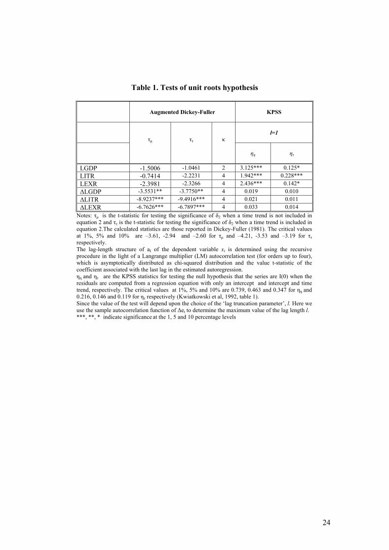
INSERT TABLE 1

Table 1 presents the results of the ADF and KPSS tests of real gross domestic

product, international tourism earnings and the effective real exchange rate. The

results of ADF test are compared with critical values we obtained from Mackinnon

(1991) tables. The results of ADF statistic for the examined time series exceed the

critical values, because the null hypothesis of a unit root is not rejected. Taking first

differences renders each series stationary, with the ADF statistics in all cases being

less than the critical value at the 1%, 5% and 10% level of significance.

The results of KPSS statistics are reported for lag – truncation parameters, since it is

unknown how many lagged residuals should be used to construct a consistent

estimator of the residual variance. The KPSS test rejects the null hypothesis of level

and trend stationarity for lag truncation parameter (l = 1)5. The KPSS statistics does

not reject the I(0) hypothesis for the first differences of the series at different levels of

∑=

=t

iit eS

1, t = 1,2,……T

The distribution of LM is non-standard: the test is an upper tail test and limiting values are provided by Kwiatkowski et al (1992), via Monte Carlo simulation. To allow weaker assumptions about the behaviour of εt, one can rely, following Phillips (1987) and Phillips and Perron (1988) on the Newey and West (1987) estimate of the long-run variance of εt which is defined as:

∑ ∑ ∑= = +=

−−− +=

T

t

l

s

T

stkiii eelswTeTlS

1 1 1

1212 ),(2)(

where w(s,l) = 1 - s / (l+1). In this case the test becomes

∑=

−=T

tt lSST

1

222 )(/ν

which is the one considered here. Obviously the value of the test will depend upon the choice of the ‘lag truncation parameter’, l. Here we use the sample autocorrelation function of ∆et to determine the maximum value of the lag length l. 5 The KPSS statistics are known to be sensitive to the choice of truncation parameter l and tend to decline monotonically as l increases. In addition the test is performed for truncation parameter. Although the statistics may differ in the level of significance, the qualitative result remains the same.

14

significance. Therefore, the combined results from both tests (ADF, KPSS) suggest

that all the series under consideration appear to be integrated of order 1, I(1).

4. Cointegration test

Following the maximum likelihood procedure of Johansen (1988) and Johansen and

Juselious (1990), a p-dimensional (p×1) vector autoregressive model with Gaussian

errors can be expressed by its first-differenced error correction form as:

∆Υt = µ + Γ1 ∆Υt-1+ Γ2 ∆Υt-2 +…..+ Γp-1∆Υt-p+1 + ΠΥt-1 + ut (8)

where:

Υt is a p×1 vector containing the variables.

µ is the p×1 vector of constant terms.

Γi = -I + A1 + A2 +…..+ Ai (i =1,2…,p-1) is the p×p matrix of coefficients.

Π = I - A1 -A2 -…..- Ap is the p×p matrix of coefficients.

ut is the p×1 vector of the disturbance terms coefficients.

The Π matrix conveys information about the long-run relationship between Yt

variables and the rank of Π is the number of linearly independent and stationary linear

combinations of variables studied. Thus, testing for cointegration involves testing for

the rank of Π matrix r by examining whether the eigenvalues of Π are significantly

different from zero. Johansen (1988) and Johansen and Juselious (1990) propose two

test statistics for testing the number of cointegrating vectors (or the rank of Π) in the

15

VAR model. These are the trace (Tr) test and the maximum eigenvalue (L-max) test.

The likelihood ratio statistic for the trace test is:

)ˆ1ln(ln21

i

p

riTQ λ∑

+=

−−=− (9)

where λ r+1, ……., λ p are the estimated p - r smallest eigenvalues. The null hypothesis

to be tested is that there are at most r cointegrating vectors. That is, the number of

cointegrating vectors is less than or equal to r, where r is 0,1, or 2…., and so forth. In

each case, the null hypothesis is tested against the general alternative.

Alternatively, the L-max statistic is:

)ˆ1ln(ln2 1+−−=− rTQ λ (10)

In this test, the null hypothesis of r cointegrating vectors is tested against the

alternative hypothesis of r+1 cointegrating vectors. Thus, the null hypothesis r = 0 is

tested against the alternative that r = 1, r = 1 against the alternative r = 2, and so

forth. It is well known the cointegration tests are very sensitive to the choice of lag

length. The Schwarz Criterion (SC) and the likelihood ratio test are used to select the

number of lags required in the cointegration test.

INSERT TABLE 2

The results that appear in Table 2 suggest that the number of statistically significant

normalized cointegration vectors is equal to 1 and are the following:

16

LGDP = O.31290LITR + 4.8690LEXR (11)

From the above cointegrated vector we can infer that in the long-run tourist earnings

and real exchange rate have a positive effect on gross domestic product. The two

other cointegrated vector models presented the same positive relationship when the

real exchange rate and international tourism earnings were used as a dependent

variable.

According to the signs of the vector cointegration components and based on the basis

of economic theory the above relationships can be used as an error correction

mechanism in a VAR model.

5. A VAR model with an error correction mechanism

After determining that the logarithms of the model variables are cointegrated, we

must estimate then a VAR model in which we shall include a mechanism of error

correction model (MEC). The error correction model (equation 3) is used to

investigate the causal relationships among the variables real gross domestic product,

international tourism earnings and the effective real exchange rate (GDP, ITR, EXR).

Such analysis provides the short – run dynamic adjustment towards the long – run

equilibrium. The significance levels of the F – statistics for the lagged variables and

the t – statistics for the coefficient δ of ECt-1 are used to test for Granger causality.

The numbers in parentheses are the lag lengths determined by using the Akaike

criterion.

17

As discussed earlier in section 2, there are two channels of causality Granger (1988).

These are called channel 1 and channel 2. If lagged values of a variable (except the

lagged value of the dependent variable) on the right hand side in equation 3 are jointly

significant then this is channel 1. On the other hand, if the lagged value of the error

correction term is significant, then this is channel 2. The results are summarized in

table 3.

INSERT TABLE 3

For convenience in discussing the results, let us call the relationships a “strong causal

relation” if it is through both channel 1 and channel 2 and simply a “causal relation” if

it is through either channel 1 or channel 2.

From the results of table 3 we can infer that coefficient δ is statistically significant

only in case we use economic growth as an endogenous variable so we have then the

channel one which means that international tourism earnings and real exchange rate

effect on economic growth. Also, the coefficients of lagged variables are statistically

significant in case that economic growth and international tourism earnings are used

as a dependent variable (channel 1), which means that economic growth and real

exchange rate effect on international tourism earnings.

The results of table 4 present causality test through these channels

INSERT TABLE 4

From the results of Table 4 we can infer that there is a “strong Granger causal”

relation between international tourism earnings and economic growth, there is a

“strong causal” relation between real exchange rate and economic growth, while the

relation between economic growth and international tourism earnings is simply a

18

“causal relation” and lastly the relation between real exchange rate and international

tourism earnings is simply a “causal relation” as well.

6. Concluding remarks

In this paper an effort was made in order to examine the relationship among

international tourism earnings, real exchange rate and economic growth in one tourist

country par excellance, such as Greece, through the analysis of multivariate causality

based on an error correction model. For empirical testing of these variables, we used

the Johansen cointegration test and then Granger causality tests based on a vector

error correction model.

The results of the cointegration analysis suggest the existence of cointegration

relationship between the three variables. This indicates the presence of common trend

or long-run relationships among these variables.

The results of the causality analysis denote that international tourism earnings and real

exchange rate cause economic growth with a “strong causal” relationship, while

economic growth and real exchange rate cause international tourism earnings with a

“simply causal” relationship.

Since the hypotheses set at the beginning of this paper have been answered, as a final

concluding remark we can infer that the significant impact of tourism on the Greek

economy justifies the necessity of public intervention aimed, on the one hand, at

promoting and increasing tourism demand, and, on the other hand, providing and

fostering the development of tourism supply. The intense state intervention for

tourism growth and especially for tourist economy, arises either directly from the

performance of tourist infrastructure works or indirectly from the mechanism of funds

and incentives. Generally, this is a characteristic feature of modern tourism, but also it

19

is factual evidence that the state tries to develop tourism, which is regarded as one of

the most important sectors of economic activity.

ACKNOWLEDGEMENTS The author is very grateful to an anonymous referee for useful suggestions References

Akaike, H. (1974), A New Look at the Statistical Model Identification, IEEE

Transaction on Automatic Control, AC-19, 716 - 723.

Balaguer, J and Cantavella-Jorda, M. (2002), Tourism as a Long-run Economic

Growth Factor: The Spanish Case, Applied Economics, Vol 34, 877 - 884.

Bhagwati, J and Srinivasan, T. (1979), Trade Policy and Development, in

International Economic Policy: Theory and Evidence, (Eds) R. Dornbunsch and J.

Frenkel, Johns Hopkins University Press, Baltimore, 1 - 35.

Cooley, T. F, and LeRoy, S. F. (1985). A Theoretical Macroeconomics: A Critique,

Journal of Monetary Economics, Vol. 16, 283 – 308.

Dickey, D.A., and Fuller, W.A. (1979), Distribution of the Estimators for

Autoregressive Time Series with a Unit Root, Journal of the American Statistical

Association, Vol 74, 427 – 431.

20

Dickey, D.A., and Fuller, W.A. (1981), Likelihood Ratio Statistics for Autoregressive

Time Series with a Unit Root, Econometrica, Vol 49, 1057 – 1072.

Dritsakis, N, and Athanasiadis, S., (2000), An Econometric Model of Tourist

Demand: The Case of Greece, Journal of hospitality & leisure marketing, Vol. 2, 39 -

49.

Engle, R. F, and, C. W. J Granger (1987). Cointegration and Error Correction:

Representation, estimation and testing. Econometrica, 55, 251 – 276.

Engle, R.F. and Yoo, B.S. (1987), Forecasting and Testing in Cointegrated Systems,

Journal of Econometrics, Vol 35, 143 – 159.

Granger, C., (1988), Some Recent Developments in a Concept of Causality. Journal

of Econometrics, Vol 39, 199 – 211.

Hazari, B.R and Kaur, C. (1995), Tourism and Welfare in the Presence of Pure

Monopoly in the Non-traded Goods Sector, International Review of Economics and

Finance, Vol 4, 171 - 177.

Hazari, B.R., and Ng, A. (1993), An Analysis of Tourists’ Consumption of Non-

traded Goods and Services on the Welfare of the Domestic Consumers, International

Review of Economics and Finance, Vol 2, 3 - 58.

21

Hazari, B.R and Sgro, P.M. (1995), Tourism and Growth in a Dynamic Model of

Trade, The Journal of International Trade and Economic Development, Vol 4, 253 -

256.

Ηelpman, E., and Krugman, P. (1985), Market Structure and Foreign Trade, MIT

Press, Cambridge.

Johansen, S (1988), Statistical Analysis of Cointegration Vectors, Journal of

Economic Dynamics and Control, Vol 12, 231 – 254.

Johansen, S., and Juselious, K. (1990), Maximum Likelihood Estimation and

Inference on Cointegration With Applications to the Demand for the Money, Oxford

Bulletin of Economics and Statistics, Vol 52, 169 - 210.

Johansen, S. (1995). Likelihood – Based Inference in Cointegrated Vector

Autoregressive Models, Oxford University Press, Oxford.

Komiya, R. (1967), Non-traded Goods and the Pure Theory of International Trade,

International Economic Review, Vol 8, 132 - 152.

Krueger, Α. (1980), Τrade Policy as an Input to Development, American Economic

Review, Vol 70, 188 - 292.

22

Kwiatkowski, D., Phillips, P.C., Schmidt, P. and Shin, Y. (1992), Testing the Null

Hypothesis of Stationarity Against the Alternative of a Unit Root, Journal of

Econometrics, Vol 54, 159 - 178.

Lim, C. and McAller (2000). A Seasonal Analysis of Asian Tourist Arrivals to

Australia. Applied Economics, 32, 499 – 509.

Μckinnon, R. (1964), Foreign Exchange Constrain in Economic Development and

Efficient Aid Allocation, Economic Journal, Vol 74, 388 - 409.

Mackinnon, J. (1991), Critical Values for Cointegration Tests in Long-run Economic

Relationship in Readings in Cointegration (eds) Engle and Granger, Oxford

University Press, New York, 267 - 276.

Nelson, C.R. and Plosser, C.I. (1982), Trends and Random Walks in Macroeconomic

Time Series: Some Evidence and Implications, Journal of Monetary Economics, Vol

10, 139 - 162.

Newey, W. and West, K. (1987), A Simple, Positive Semi – Definite, Heteroske-

dasticity and Autocorrelation Consistent Covariance Matrix, Econometrica, Vol 55,

703 – 708.

Osterwald – Lenum, M (1992). A Note With Quantiles of the Asymptotic Distribution

of the Maximum Likelihood Cointegration Rank Test Statistics, Oxford Bulletin of

Economics and Statistics, 54, 461 – 472.

23

Papatheodorou, A. (1999), The Demand for International Tourism in the

Mediterranean Region, Applied Economics, Vol 31, 619 – 630.

Payne, J and Mervar, A. (2002), A Note on Modeling Tourism Revenues in Croatia,

Tourism Economics, Vol 8, No 1, 103 - 109.

Phillips, P.C. (1987), Time Series Regression With Unit Roots, Econometrica, Vol 2,

277 – 301.

Phillips., P.C., and Perron, P. (1988), Testing for a Unit Root in Time Series

Regression, Biometrika, Vol 75, 335 - 346.

Runkle, D. (1987). Vector Autoregressive and Reality, Journar of Economic and

Business Statistics, Vol. 5, 437 – 454.

Sims, C. A. (1980). Macroeconomics and Reality. Econometrica, Vol. 48, 1 – 48.

24

Table 1. Tests of unit roots hypothesis

Augmented Dickey-Fuller

KPSS

l=1

τµ

ττ

κ

ηη

ητ

LGDP -1.5006 -1.0461 2 3.125*** 0.125* LITR -0.7414 -2.2231 4 1.942*** 0.228*** LEXR -2.3981 -2.3266 4 2.436*** 0.142* ∆LGDP -3.5531** -3.7750** 4 0.019 0.010 ∆LITR -8.9237*** -9.4916*** 4 0.021 0.011 ∆LEXR -6.7626*** -6.7897*** 4 0.033 0.014

Notes: τµ is the t-statistic for testing the significance of δ2 when a time trend is not included in equation 2 and ττ is the t-statistic for testing the significance of δ2 when a time trend is included in equation 2.The calculated statistics are those reported in Dickey-Fuller (1981). The critical values at 1%, 5% and 10% are –3.61, -2.94 and –2.60 for τµ and –4.21, -3.53 and –3.19 for ττ respectively. The lag-length structure of aΙ of the dependent variable xt is determined using the recursive procedure in the light of a Langrange multiplier (LM) autocorrelation test (for orders up to four), which is asymptotically distributed as chi-squared distribution and the value t-statistic of the coefficient associated with the last lag in the estimated autoregression. ηη and ητ are the KPSS statistics for testing the null hypothesis that the series are I(0) when the residuals are computed from a regression equation with only an intercept and intercept and time trend, respectively. The critical values at 1%, 5% and 10% are 0.739, 0.463 and 0.347 for ηη and 0.216, 0.146 and 0.119 for ητ respectively (Kwiatkowski et al, 1992, table 1). Since the value of the test will depend upon the choice of the ‘lag truncation parameter’, l. Here we use the sample autocorrelation function of ∆et to determine the maximum value of the lag length l. ***, **, * indicate significance at the 1, 5 and 10 percentage levels

25

Table 2. Cointegration tests based on the Johansen and Johansen and Juselious

approach (LGDP, LITR, LEXR, VAR lag = 4) Trace test 5% critical value 10% critical value

H0: r = 0 42.1185 24.0500 21.4600 H0: r ≤ 1 4.3561 12.3600 10.2500 H0: r ≤ 2 1.6837 4.1600 3.04000

Notes: • Critical values are taken from Osterwald – Lenum (1992). • r denote the number of cointegrated vectors. • Schwarz Criteria (SC) was used to select the number of lags required in the cointegration test. The computed

Ljung – Box Q – statistics indicate that the residuals are white noise.

Table 3 – Causality test results based on vector error – correction modeling F – significance level Dependent

Variable ∆LGDP ∆LITR ∆LEXR t – statistic

u t-1

∆LGDP 0.236 (2) 0.001***(2) 0.008*** (1) -4.1763*** ∆LITR 0.013** (3) 0.346 (3) 0.009*** (2) -1.2897 ∆LEXR 0.198 (2) 0.137 (2) 0.145 (1) -1.0845

Notes: * , **, and *** indicate 10%, 5%, and 1% levels of significance. Number in parentheses are lag lengths.

Table 4 – Summary of causal relations LGDP→LITR LGDP →LEXR LITR → LGDP LITR → LEXR LEXR→LGDP LEXR→LITR

1 1,2 1,2 1