Toward Gage R&R Guidelines for - pomsmeetings.org Gauge R&R Guidelines for Statistically Designed...

Bagchi and Rajmani, POMS 2010

1

Toward Gauge R&R Guidelines for Statistically Designed Experiments

Tapan P Bagchi

VGSOM/IEM, IIT Kharagpur, Kharagpur 721302, India

[email protected]

Rajmani Prasad

IEM, IIT Kharagpur, Kharagpur 721302, India

[email protected]

Abstract

With today’s push for Six Sigma, the issue of measurement errors in quality assurance is

now widely discussed and as a result naive to theoretically sophisticated suggestions have

emerged. This has led to formulating Gauge R&R guidelines by AIAG and others for the

recommended choice and use of gauges to measure product characteristics. This paper

extends that effort, linking the overall power of ANOVA tests in DOE to the number of

treatments employed, parts produced in each treatment, and measurements taken on each

part. It invokes Patnaik’s work (1949) to explore how these quantities may be optimized

while conducting DOE to achieve a pre-stated detection power.

1. Introduction

Patnaik (1949) observed that in the Neyman-Pearson theory of testing statistical

hypotheses the efficiency of a statistical test should be judged by its power of detecting

departures from the null hypothesis. Patnaik then presented a methodology that provides

approximate power functions for variance-ratio tests that involve the noncentral F

distribution. These results focused on deriving approximations to the noncentral F (called

F ) distribution to permit one to calculate, for example, the probability of rejecting the

null hypothesis when it is false in a variance-ratio test with specified significance (),

deviation and the number of replicated observations. Subsequently these approximations

led to the development of the Person-Hartley tables and charts that relate the power of the

variance-ratio test to a specified deviation or noncentrality (Pearson and Hartley 1972).

The data are analyzed by ANOVA (Dean and Voss 1999; Montgomery 2007). The

present work extends these results to tackle situations where observations are imperfect

implying that the data are affected by measurement errors.

Applications of statistically designed experiments currently abound, not only in

academic and R&D studies, but also in process improvement practices and approaches

such as the Six Sigma DMAIC (Pyzdek 2000). As Montgomery notes, experiments are

performed as a test or series of tests in which purposeful changes are made to certain

experimental factors with the objective to observe any changes in the output response.

The observed data are statistically analyzed to lead to statistically valid and objective

conclusions at the end of the investigation. Perhaps the only guidelines on judging the

mailto:[email protected]

mailto:[email protected]


2

adequacy of measuring systems that are available to practitioners of quality control are

those by AIAG. To experimentalists the AIAG guidelines are grossly inadequate for they

do not prescribe how data should be collected to lead to credible and statistically

defensible conclusions. As a result, for example, many experiments use as few as only

two replications while some clinical trails may use too many (Donner 1984). The

investigator is generally silent about measurement errors and often uses only a single

measurement per sample.

As Simanek (1996) has said, no measurement is perfectly accurate or exact, hence

even in conducting designed experiments we can never hope to measure true response

values. The true value is the measurement if we could somehow eliminate all errors from

instruments and hold steady all factors other than those being experimentally manipulated.

Generally such observed data combine in them what is commonly called ―experimental

errors‖ that include the effect or influence of all factors—other than factors that the

investigator manipulates. Improperly designed experimental studies conducted in such

operating environment introduce unknown degrees of errors in conclusions drawn from

them. Indeed a measurement or experimental result is of little use if nothing is known

about the size of its error content.

The flaws of the ramshackle ways for conducting multi-factor investigations was

recognized formally by Fisher (1958), who introduced the principles behind planning

experiments that guide empirical studies today. Various enhancements followed Fisher’s

work. Process sample sizes for the ANOVA scheme for measurement error-free

conditions (measurement errors being distinct from the experimental errors noted above)

were studied by Fisher (1928), Tang (1938), Patnaik (1949), and Tiku (1967) and several

others. Sample size specification answers one of the first questions an investigator would

face in designed experimental studies (DOE)—―how many observations do I need to

take?‖ or ―Given my limited budget, how can I gain as much information as possible?‖

However, methods for sample size determination in DOE (that do not explicitly consider

measurement errors) abound. Pearson and Hartley (1972), Dean and Voss (1999) and

Montgomery (2007) describe these. Note the distinction we deliberately make here

between errors in data that are introduced by an imperfect measurement system in use as

opposed to those caused by uncontrolled experimental conditions.

2. A Quick Overview of One-way ANOVA

An investigator in his inquiry about the behavior of how a system, be it in natural or

physical sciences, resorts to experimentation except in two situations. The first are ones

when he is unable to identify the key factors that might be influencing the response, as in

the domains of economics, meteorology or psychology. In these situations a DOE

scheme cannot be set up; one must merely observe the phenomena and look for any

notable relationships. The second situation is when our knowledge has already progressed

to the point that a theoretical model of the cause-effect relationship may be developed

from theoretical considerations alone. This is common, for instance, in electrical

sciences. In the remaining situations whose number is large one approaches the quest

through scientifically planned empirical investigations guided by DOE. Use of DOE is

most common in metallurgy, chemistry, new product development, drug trials, process

yield improvement and in the optimization of computational algorithms (Bagchi 1999).


3

Montgomery (2007) explains the principles (owed to Fisher 1928) of statistically

designed experiments. In such experiments one begins with a statement of the cause-

effect phenomenon to be investigated, a list of factors to be manipulated and their levels

(called treatments), selecting the response variable, and a considered choice of the

experimental design or plan. One then conducts the experiments as guided by the design,

performs data analysis, and sums up the conclusions and recommendations. Numerous

different schemes or designs are now available that can help serve widely varying

investigative purposes, including optimization of the response. Box (1999), Draper

(1982), Taguchi (1987) and many others have proposed some highly useful methods to

study systems for which first principles do not easily lead to determining the input-

response relationship.

The simplest statistical experiment comprises one single factor whose influence on a

response of interest is to be experimentally studied. To do this one conducts trials when

the factor is set at two or more distinct ―treatment‖ levels and the trial is run multiple

times at each treatment level. The corresponding response is observed. Multiple trials

(called replications of the experiment) at each factor treatment are needed here to help

accomplish a statistically sound analysis of the observed data. Replication serves two

purposes. First it allows the investigator to find an estimate of the experimental error—

the influence on the response of all other factors (ambient temperature, vibration,

measurement errors, etc. ) that are not in control during the experiments. The error thus

estimated forms a basic unit of measurement to determine whether the observed

differences among results found at different treatment levels are statistically significant.

The second purpose of replication is to help estimate such treatment or factor effects

more precisely. For details we refer the reader to Montgomery (2007) or Dean and Voss

(1999). For our immediate purpose we outline the data analysis procedure used in single-

factor studies known as one-way ANOVA.

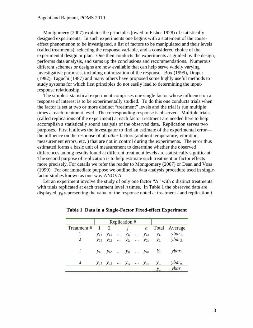
Let an experiment involve the study of only one factor ―A‖ with a distinct treatments

with trials replicated at each treatment level n times. In Table 1 the observed data are

displayed, yij representing the value of the response noted at treatment i and replication j.

Table 1 Data in a Single-Factor Fixed-effect Experiment

Replication #

Treatment # 1 2 j n Total Average

1 y11 y12 … y1j … y1n y1. ybar1.

2 y21 y22 … y2j … y2n y2. ybar2.

.

i yi1 yi2 … yij … yin Yi. ybari.

.

a ya1 ya2 … yaj … yan ya. ybara.

y.. ybar..


4

Table 1 employs the notations

n

j

iji yy1

. nyybar ii /.. i = 1, 2, …, a

n

j

ij

a

i

yy11

.. )/(.... anyybar

The observed response data {yij} are analyzed using the one-way ANOVA procedure

based on the assumption that the response y is affected by the varying treatment levels of

the single experimental factor, and also by the uncontrolled factors. The relationship is

modeled as

yij = i + ij, i = 1, 2, …, a; j = 1, 2, …, n (1)

where i is the treatment mean at the ith

treatment level and ij is a random error

incorporating all other sources of variability including measurement errors and

uncontrolled factors. Relationship (1) may also be written as the means model, i = + i,

i = 1, 2, …, a, a procedure that converts (1) into the ith

treatment model or effects model,

yij = + i,+ ij, i = 1, 2, …, a; j = 1, 2, …, n (2)

Treatment effects of factor A are evaluated by setting up a test of hypothesis, with

H0: 1 = 2 = … = a

H1: j for at least one pair (i, j) of treatment effects.

Since is the overall average, it is easy to see that 1 + 2 + … + a = 0. The hypotheses

H0 and H1 may be then re-stated as

H0: 1 = 2 = … = a = 0

H1: i for at least one i.

The hypotheses are tested for their acceptability by constructing the classical sums-of-

squares and the mean-sums-of-squares quantities in one-way ANOVA. To complete

ANOVA one uses quantities defined and computed as follows.

a

i

iTreatments ybarybarnSS1

2

... )(

MSTreatments = SSTreatments/(a-1)

a

i

ij

n

j

Total ybarySS1

2

..

1

)(


5

SSE = SSTotal – SSTreatments and

MSE = SSE/(n(a – 1))

The test statistic F0 (when hypothesis H0 is true) is defined as MSTreatments/MSE. F0

follows the F distribution with degrees of freedom (a – 1), n(a – 1). If the null hypothesis

were true, this statistic would have a value Fwhen is the significance (the

probability of rejecting H0 when it is true, or a type I error) of the test.

A type II error is committed in the one-way ANOVA procedure when H0 is false, i.e.,

when at least one treatment effecti is not zero, yet due to randomness F0 F. The

probability of committing a type II error is denoted by , and the quantity (1 – ) is called

the detection power of the test. The power of a statistical test is defined as the ability of

the test when it should reject the null hypothesis when the null hypothesis is false. This

present study delves into the evaluation of power in statistical experiments when it is

affected by the number of replicates that reflect process or part variability, as well as the

number of measurements taken on each part experimentally produced under different

treatment conditions.

3. The Issue of Sample Size in One-way DOE

Gill (1968) in establishing sample size for experiments on cow milk yield confronted a

problem typical in sample size determination in designed experiments. Gill’s problem

was a one-way test in which lactational records of Holsteins, Brown Swiss, Ayrshires and

Guernsey cows were used to determine how many cows should be used to establish

differences between the largest and smallest yield means. Two classes could be

identified due to the difference in standard deviations of yield reported—Holsteins and

Brown Swiss had a standard deviation of 4.5 kg, while 3.3 was the number for Guernsey

and Jersey. The goal was to determine the number of cows to be milked to detect true

mean differences between each ―treatment level‖ (cow type) compared. The test should

have 0.5 or 0.8 power (50% or 80% chance) of detecting the specified true mean

difference in daily milk yield. Gill used the Pearson-Hartley tables to resolve that to

achieve a power of 80% 37 cows each of Holsteins and Brown Swiss would be required.

That number for comparing Guernsey and Jersey was 20 cows each, due to the latter

pair’s lower standard deviation. Nevertheless, note that Gill did not have estimates of

milk yield measurement errors when the same cow was milked on different days and milk

yield measured. Thus, he was forced to lump all sources of yield variation including

measurement errors (other than that due to treatment) into error variation. Could the

yield estimates be more precisely compared? We do not have information to answer that.

Sample size specification concerns investigators using DOE for some important

reasons. The study must be of adequate size—big enough so that an effect of scientific

significance will also be statistically significant. If sample size is too small, the

investigative effort can be a waste of resources for not having the power or capability of

producing useful results. If size is too large, however, the study will use more resources

(e.g. cows of each genre) than necessary. Hoenig and Heisy (2001) remark that in public

health and regulation it is often more important to be protected against erroneously

concluding that no difference exists when one does. Lenth (2001) remarks about the


6

relatively small amount of published literature on this issue—other than those applicable

for specific tests. The widely adopted approach for finding sample size uses the test-of-

hypothesis framework. It explicitly attempts to link power with sample size as follows.

1. Specify a hypothesis test on the unknown parameter .

2. Specify the significance level of the test.

3. Specify the effect size the detection of which is of scientific interest.

4. Obtain historical estimates of other parameters (such as experimental error

variance 2 ) needed to compute the power function of the test.

5. Specify a target power (1 - ) that you would like to assure when is outside the ±

range.

Lenth provides an insightful discussion of practical difficulties in operationalizing these

steps. He reminds, for instance, that the answer to ―How big a difference would be

important for you to be able to detect with 90% power using one-way experiments? may

be ―Huh??‖ Instead, he suggests the use of concrete questions such as ―What results

would you expect to see?‖ The answer may lead to upper and lower values of the

required sample size. As far as the method for determining sample size goes, we recall

first the procedure provided by Montgomery (2007) which in turn is based on the

methods given by Pearson and Hartley (1972) and Patnaik (1949), elaborated also by

Dean and Voss (1999) and others.

3.1 Approaches for Sample Size Determination in One-way ANOVA

Montgomery (2007) summarizes the methods for determining sample size for the case of

equal sample sizes (n) per treatment (the ―fixed effects model‖) by invoking the Pearson-

Hartley (1972) power functions as follows. The power of a statistical test (such as

experiments using one-way ANOVA for data analysis) is defined as (1 – ) where is

the probability of committing a type II error, given by

= 1 - P[reject H0 | H0 is false] = 1 – P[F0 > F, a-1,(n-1)a | H0 is false] (3)

A critical need in evaluating (3) is knowing the distribution of the test statistic F0 if the

null hypothesis H0 is false. Patnaik (1949) called the distribution of F0 (=

MSTreatments/MSE when H0 is false) a noncentral F random variable with (a – 1) and (n –

1)a degrees of freedom, and the noncentrality parameter . When = 0, the noncentral F

becomes the usual F distribution. Pearson and Hartley (1972) produced curves that relate

with another noncentrality parameter (which is related to ) defined as

2

1

2

2

a

na

i

i (4)

Pearson-Hartley curves help one determine given = 0.05 and 0.01, and a range of

degrees of freedom for the noncentral F statistic. In determining sample sizes the starting

point is the specification of . The curves also require the specification of experimental

variability 2.


7

In operationalizing the procedure, several alternate methods are adoptable. If one is

aware of the magnitude of the treatment means {i} and an estimate of 2 (as in Gill’s

milk yield tests), one can directly compute 2 and using the degrees of freedom, read off

(hence power of the test) from the Pearson-Hartley curves. If, however, the treatment

means are unknown but one is interested in detecting an increase in the standard

deviation of a randomly chosen experimental observation because of the effect of any

treatment, one may determine from the relationship

n

aa

i

i

/

/1

2

= 1)01.01( 2 Pn (5)

where P is the percent (%) specified for the increase in standard deviation of an

observation due to treatment effect beyond which one wishes to reject H0 (the hypothesis

that all treatment effects are equal). Montgomery (2007) provides several numerical

illustrations, and summarizes methods usable also for two-factor factorial fixed effect

(constant sample size) designs. It is relatively straightforward to determine Gill’s (1968)

number of required cows problem using those curves. For that study, given = 0.05, =

0.8, maximum difference detection capability of 3 kg, two treatment levels and

experimental variability = 4.5 kg one finds that one would require to use 38 cows of

each genre to compare Holsteins and Brown Swiss.

3.2 Patnaik’s (1949) Approximation for the Noncentral F Distribution

Patnaik noted that the power function (1 - in our notation) for the F distribution may be

used to determine in advance the size of experiment (number of samples required) to

ensure that a worthwhile difference () would be established as significant—if it exists.

He further remarked that the mathematical forms of these distributions were long known,

but due to their complexity, computing the power tables based on them was not easy. To

this end Patnaik developed approximations to the probability integrals involved here and

coined the terms noncentral -square and noncentral F.

The noncentral F is denoted by Patnaik as F , which he approximated by fitting an F

distribution whose first two moments are identical to those of F , a procedure that was

subsequently adopted to construct the power and operating characteristic curves of

ANOVA power functions by Pearson and Hartley (1972). Only the parts of Patnaik’s

procedure relevant to the present context are extracted below. For a detailed description

the reader is referred to Patnaik (1949) and to the text portions of Pearson and Hartley.

Before proceeding further, however, we note that in the discussions so far, the well-

known result is established and then invoked multiple times—increase in sample size in

each treatment in a designed experiment increases the power of the test. However,

experimental error variability measured either as standard deviation or experimental

variance 2 is not explicitly considered in any of the data analysis or measurement system

selection procedures while conducting DOE. Their absence in DOE literature is

conspicuous. Rather, although measurement errors are acknowledged, suggestions are

made only to ―keep their impact low‖ wherever measurements are used, be it in


8

manufacturing, process improvement, or in cause-effect studies (Juran and Gryna 1993;

AIAG 2002). What follows is a recap of how measurement errors are estimated and

quantified—hopefully before the instruments are applied in practice to evaluate critical-

to-quality (CTQ) product characteristics. The inadequacy of such suggestions is self

evident if one looks at the different ways the observed experimental data (the input)—

even in a carefully completed one-way ANOVA—can be affected. This is depicted in

Figure 1. The notations used are shown in Table 2. Whether the issue of measurement is

serious enough to be considered in power projections can be inferred from the presently

published prescription (AIAG guidelines) that states that measurement variances

quantified as 2

Gauge R&R ―up to a third of the variance of the process being measured‖ are

―acceptable‖ (AIAG 2002; Wheeler 2009). However, note that at this level of

measurement system performance one has little idea about detectabilty (based on ) and

the extent to which type II errors are committed by plant and R&D staff.

Figure 1 Constituents of Variance in Experimental Data

Table 2 Variability in Experimental data

Variance Source of variability in data 2

variabilitytotal Total data variability resulting from all sources of variation

2

treatment Variability caused by treatment effects

2

variabilityparttoparttrue True process variability

2

variabilityprocessobserved Observed variability in experimental data, 2 in this paper

2

variabilitytmeasuremen Variability caused by the measurement system—includes

repeatability, bias, stability and reproducibility

2

variabilityprocessobserved

2

variabilitytmeasuremen

2

variabilitytotal 2

variabilityprocessorparttoparttrue

2

treatment


9

4. Measurement Errors and Gauge R&R

In experimental investigations one is invariably interested in good precision (defined

as the closeness of repeated evaluation of the same object), which depends on the

variability of the experimental material, number of experimental units (the sample size in

one-way ANOVA), the number of repeated observations per unit and the performance of

the primary instruments. As stated, the ANOVA procedure helps draw inferential

conclusions on the basis of the experimental error, also called the residual error. The raw

data observed contains a total variability that Fisher (1966) showed could be decomposed

into several different sources of variability as indicated by Figure 1 and Table 2. Such

breakdown of variability could be the basis for deciding how to optimally allocate the

available resources to replicated process runs (producing several parts or process samples

at identical experimental or treatment settings) on one hand and repeating measurements

on the same part on the other. The object would be to expend minimum resources that

would ensure that treatment effects the specified detection level are not overlooked.

Note that both replication and/or repetition of measurements at various levels of the

experiment can increase precision, though the cost of an additional experimental unit or

the number of an additional measurement taken would in general not be identical,

begging for their estimation and optimization to provide protection against drawing

wrong conclusions from the experiments run.

Juran and Gryna (1993) remarked that even when used correctly, a measuring

instrument may not give a true reading of a (quality) characteristic. Results may be

affected by precision, and by bias. They note that if measurement errors are large, the

findings of the process must be analyzed before proceeding with interventions such as

quality improvement initiatives. The components of variability in a measurement system,

assuming that one has taken care of bias by calibration and stability by suitable methods,

are gauge repeatability and reproducibility. Such variability may be estimated by

conducting Gauge R&R studies discussed widely in contemporary texts of quality

assurance (Juran and Gryna 1993; Montgomery 2002; Mitra 2009).

The primary aim of these procedures is to help estimate two key components of

measurement errors—gauge repeatability, and gauge reproducibility. The first—

repeatability—represents the inherent variation of the measuring device as it is repeatedly

used by the same operator on the same object. The second error component is

reproducibility, the variability that is observed when different operators measure different

objects with the same gauge. The gauge R&R procedure produces estimates of the total

error variance due to the measurement system comprising measurement methods, gauges

and operators using them. In Figure 1 this variance is represented by 2

variabilitytmeasuremen .

The procedure for estimating this variance follows either the ―range‖ method, or the

ANOVA method, both being well documented (Montgomery 2002).

Gryna, Chua and Defeo (2007) remark that when 2

variabilitytmeasuremen and therefore the

total standard deviation of repeatability and reproducibility is known, one must judge the

adequacy of the measurement process. Authors cite rules-of-thumb that practitioners

commonly use here, such as if 5.15 iabilitytmeasuremen var specification range of the quality

characteristic being measured, the measurement process is acceptable, not otherwise.

However, such rules beg rendering them to be more precise. Similarly, AIAG Guidelines


10

(AIAG 2002) do not indicate the extent of type II errors one is likely to commit if one

follows the stipulated guidelines to plan statistical experiments.

Among other things, the present work uses Patnaik’s approximations to develop the

quantitative link between type II errors and (a) number of treatments used in an

experiment analyzed by one-way ANOVA, (b) the number of replicated process samples

(parts) required at each treatment, and (c) the number of measurements to be made per

part. The outcome is an estimate of the overall risk (1 - ) of failing to find a target

treatment effect that should be detected. It is also shown here that one is often able to

enjoy the overall protection against wrong decisions without upgrading to sophisticated

measurement technologies that give very low iabilitytmeasuremen var —by producing additional

part samples, and/or by making extra measurements per part.

5. A Method for Determining Process and Measurement Sample Sizes

A look at Figure 1 will clarify that the different effects of the constituent variances of

the overall (total) variance of the data produced by a measurement system are additive,

ignoring interaction and higher order effects that may be estimated with appropriately

planned ANOVA when one is thus inclined. Interactions between operators, parts, and

measurements, can actually be estimated, but are typically found to be negligible (see

pages 384-387, Montgomery 2002). For the present we ignore interactions and instead

focus on determining the critical sample sizes for a well-planned set of experiments to

ensure a pre-stated level of protection against wrong conclusions. In the illustrated

derivation that follows we assume that one is conducting a single-factor experiment

utilizing multiple treatments and analyzing the data using one-way ANOVA.

The overall objective in this undertaking is to determine the quantitative dependency

of failing to detect a specified level of treatment effect to the number of process samples

(henceforth called ―parts‖) produced in each treatment in a fixed effect design and to the

number of measurements one would make on each part. The overall protection this

procedure would afford may be written as

Overall Power of the experiment = (1 - treatment)(1 - measurement) (6)

To operationalize this procedure for estimating the overall power one would need to

answer the two questions—(1) how many parts to produce during a treatment, and (2)

how many measurements to take per part. Figure 1 provides the basis for answering

these two questions, if one invokes Patnaik’s approximation for the noncentral F. To

proceed we first set up a table modified over Table 1 to incorporate the measurement

process. In this modified scheme each part produced will be measured m times. Thus,

instead of a single observation yij in the (i, j) cell as shown in Table 1 we shall have m

entries in it as

yijk, i = 1, 2, …, a; j = 1, 2, …, p and k = 1, 2, …, m

Here p parts are produced in each treatment. Thus the two sample sizes of interest here

are p (the number of replicated parts produced in each treatment) and m (the number of


11

measurements made per part). These two quantities are our decision variables in

optimizing the overall type II error or the overall power of the experiment.

Let us now illustrate the well known procedure for estimating the required number of

measurements/part when the measurement system variance 2

variabilitytmeasuremen is not

known. The goal here will be to have sufficient power through a minimum number (m)

of measurements that would be able to detect through measurements a change of P% in

the average of measured data due to variability in measurements. Using (5) which was

obtained from Montgomery (2007, page 109), also given in Pearson and Hartley (1972,

page 159) one finds

1)01.01( 2Pm

For a numerical problem in which the number of parts used in each treatment (p) and

the desired significance are known, for given m and P one can find the corresponding

value of and then the probability of committing a type II error () from the Pearson-

Hartley charts given in Montgomery (2007, page 247 onward), or from Pearson and

Hartley (1972, Table 30). For example, if p = 5, P = 10% and a trial value of m is

assumed to be 5, one computes the degrees of freedom for the noncentral F to be 1 = p –

1 = 4 and 2 = m(p – 1) = 20. These quantities lead to = 1)1.01(5 2 or 1.025.

Let = 0.05. Then from the Pearson-Hartley chart one obtains 1 - = 0.55 yielding a

power of 0.55. Similarly, by assuming m = 10 and visually interpreting the curves one

obtains a power of 0.72. For m = 20 one obtains a power of 0.96. This process of

gradually adjusting the trial value of m can continue till one reaches the target power.

In a similar manner the number of parts required to detect a change in average part

dimension due to treatment effects can be found. Suppose we wish to detect a Q%

increase in the standard deviation of the variability due to treatment effects. The problem

then becomes one of finding the required number of parts. In this case

1)01.01( 2Qp

Again, given the number of treatments a, one finds 1 = a – 1 and 2 = p(a – 1). When

significance is specified, for a starting value for the number of parts (p) one can

calculate , and then the corresponding power of detecting treatment effects (1 - ) from

the Pearson-Hartley charts. The process may be repeated with different values of p till a

value is located that can deliver the required target power.

The procedure described above has one important utility. It assures specified powers

for the experiment’s ability to detect average part size differences, and also separately

detect treatment effects on those parts—without the knowledge of measurement system

variability or process variability. The detection targets embedded in the forms of P or Q

assure catching a relative increase of the standard deviation of observations, separately

for measurements, and for the needed replications. However, frequently it is necessary to

determine the overall error one may commit or the risk () one might be exposed to,

while conducting designed experiments with repeated measurements. For this it is


12

necessary to obtain prior estimates of measurement variability 2

variabilitytmeasuremen and the

observed process or part-to-part variability 2

variabilityprocessobserved . The procedure would be

as follows.

One begins with (4). Montgomery (2003) shows that the smallest value of 2

corresponding to a specified difference D between any two treatment means is given by

2

22

2

a

nD (7)

Dean and Voss (1999, page 52) provide the proof of (7). Recall from Section 3.1 that

that the distribution of F0 (= MSTreatments/MSE when H0 is false) a noncentral F random

variable with (a – 1) and (n – 1)a degrees of freedom. Hence, given the number of

treatments a, the power of the test would depend on sample size n and D and would be

evaluated using the noncentral F distribution, F . Power itself is evaluated as

1 - = P[MSTreatments/MSE > F’a-1, (n – 1)a, ]

Here F a-1, (n – 1)a, is the critical value of the noncentral F random variable for

significance . Thus the steps to determine the power of the one-way ANOVA as a

function of the number (n) of parts or process samples would be as follows.

1. Estimate 2

variabilityprocessobserved , the observed part-to-part variance from historical

data.

2. Decide on number of treatments a, treatment effect detection criterion D and

significance .

3. Select n. Hence for the noncentral F distribution to be used, the degrees of

freedom would be (a – 1), and a(n – 1).

4. Using 2

variabilityprocessobserved for 2 and (7) calculate the noncentral quantity

2, and

hence .

5. Use the appropriate Pearson-Hartley curves (Pearson and Hartley 1972, Table 30)

to read off the power of the test—the probability of rejecting the hypothesis (that

all a treatment effects are identical) at detection criterion D.

In finding the minimum sample size n to achieve a target power (1 - ) of the one-way

ANOVA the steps 3 to 5 are recursively run. One begins with a trial value of n and

determines the corresponding power. If the result is lower than the target power desired,

one increases n in successive iterations of the steps above till the resulting power target

power. Note from Figure 1 that the observed process (i.e., part-to-part) variance 2

variabilityprocessobserved includes the effect of measurement errors, hence the number of parts

thus estimated is conservative (higher than what would result from using true part-to-part

variance).

Patnaik (1949) provided an approximation to the noncentral F (i.e., F ) distribution

that leads one to directly evaluate the critical value of F using statistical built-in


13

functions in software tools such as Excel

for the standard F distribution. This thus

bypasses the need to visually interpret quantities from Table 30 of Pearson and Hartley

(1972). This method, described below, was extensively used in the present study to help

estimate the different required sample sizes.

5.1 Patnaik’s Approximation of the noncentral F Distribution

Patnaik (1949) suggested that the noncentral F distribution ( F ) can be approximated by

a standard F distribution with some small adjustments such that the first two moments of

the two distributions are identical. This approximation saves a great deal of

computational effort, and is almost identical to the original exact quantities for most

practical purposes (Person and Hartlety 1972, page 67; Tiku 1966; Pearson and Tiku

1970). The approximation says

),(),,( 221 kFtoequalnearlyisF

where k and are determined so as to make the first two moments of the approximation

identical. Patnaik determined that

.2

)(

1

2

1

1

1

andk

In these expressions a quantity is used. It is evaluated from the relationship

)1/( 1 as shown in Pearson and Hartley (1972, page 68). Thus we have

)1( 1

2 .

6. Application of Patnaik’s Results to Sample Size Determination

Recall the conditions stated in Section 5 under which the one-way ANOVA is

conducted—the number of treatments is a, the number of replications—process samples

(parts) observed in each treatment in the fixed effect scheme of running the

experiments—is p (p 1), and each part is measured by using the measurement system

available m times (m 1). Our objective presently is to determine the minimum number

of parts that must be produced to assure sufficient power (1 - treatment) at the treatment

effect detection stage, and the number of measurements that must be obtained on each

part to ensure sufficient power (1 - measurement) in correctly determining the size of each

part measured. The two powers when multiplied—each being independent of the other as

they are operationally isolated—result in conservatively estimating the overall power of

the empirical study as stated by (6). Patnaik’s results shown in Section 5.1 may be used

in this process as follows.

Finding the required number of process samples to be collected at each treatment to

assure a power of (1 - treatment) proceeds as follows. To begin one assumes a desired

significance , the number of treatments a, the variance 2

variabilityprocessobserved (estimated

from historical process output data—this includes a small contribution of measurement


14

errors), and the target treatment effect detection capability Dt. Next a trial value of part

number p is assumed and the noncentral quantity 2 (which is based on (7)) is calculated

from the relationship

2

var

2

2

2 iabilityprocessobserved

t

a

pD

Next the degrees of freedom 1 (= a – 1) and 2 (= a(p – 1)), ))1(( 1

2 and then k

and are determined using Patnaik’s relationships

.2

)(

1

2

1

1

1

andk

As the last step, power is calculated using the relationship (Patnaik 1972, equation (66))

),(),()1( 21

1

121 1

FFPower treatment

The quantity ),( 211 F above is the one-sided critical value of the F random variable

from the ),( 211 F distribution that has (1 - ) area under the F-density to the left of

that point. This quantity can be determined, for instance, by the built-in statistical

function FINV(.., .., ..) in Excel

. (We note that in the notations used, the present paper

uses the conventional notation of for P[type II error] (Juran and Gryna 1993) while

Patnaik (1949) and Pearson and Hartley (1972) use ―‖ for power function or the ability

of the test to reject the null hypothesis when it is false.)

Thus, given p, treatment effect detection criterion Dt, significance and observed

historical process variability represented by variance 2

variabilityprocessobserved , one can

approximately calculate the power at the treatment effect detection level. Since

measurement variability is included in the observed process variability, for given p, the

power estimated as above is conservative (lower than what is possible if measurement

variability was eliminated).

The number of measurements (m) required to be taken in on each part produced to

ensure that part sizes are measured with an acceptable level of precision may be similarly

found. The following changes would be necessary. The new quantities are defined as

p = number of parts produced per treatment

Dm = target maximum detectability difference between two measurements on the same

part

a = number of treatments

m = number of measurements to be taken on each part, and 2

variabilitytmeasuremen = variance observed in measured data, estimated from gauge R&R

studies done separately


15

A key change that also occurs is how the noncentral quantity 2 is defined. In this case,

2

var

2

2

2 iabilitytmeasuremen

m

p

Dam

The rest of the procedure parallels the method used for finding the power for a given

number of parts produced in each treatment.

Thus, the present approach would allow an investigator to determine the correct

number of parts to be produced in each treatment in the experiments and the number of

measurements to be taken on each part. These together may be used in combination to

assure an overall target power of the one-way ANOVA.

7. Validation of the Method

We compare a few results of sample size determination in fixed effect one-factor

experiments that are readily available. These determine the number of process samples

(parts or experimental units) that must be used in each treatment to satisfy pre-specified

significance () and power (1 - ).

The milk yield problem of Gill (1968) involved comparison of daily milk yield of

Holstein and Brown Swiss cows (two treatments or a = 2) for whom standard deviation

of milk production (among cows of each genre) was 4.5 kg while the test specified a

detectable difference Dt equal to 3 kg. Significance was 0.05 while the number of

cows to be tested had to meet a target power (1 - ) equal to 0.8 and 0.5 respectively. No

mention was made in the problem about any imperfection in measurement. For the target

power of 0.8 the method described above produced a sample size of 38 to compare

Holsteins with Brown Swiss while Gill reported a size of 37 using plots of the power

curves. For the target power of 0.5 the computed sample size was 19 while Gill reported

18. For another two types—Guernsey and Jersey—compared, standard deviation was

3.3. For a target detectability (Dt) of 3 kg, = 0.05 and power specified at 0.8, sample

size computed was 21 while Gill determined it to be about 20 using his curves.

8. A Practical Example of Sample Size Calculation

We select a problem of sample size selection for a manufacturing process

improvement project that involved a single factor fixed effects statistical design.

Precision ball bearings (Figure 2), in order to deliver trouble-free operation for tens of

thousands of hours unattended, require the execution of very precise manufacturing

processes. Typical among these are the bearings made by SKF, Dynaroll

, and others

who make a wide variety of bearings classified as ABEC models 1 to 9. These models

steadily increase in precision spanning applications from roller skates to supporting

rotating shafts in modern Jets and spacecraft. A plant producing ABEC 5 class of

bearings was incurring about 1% internal failure losses and it felt that it had poor control

on its ring grinding process. A Six Sigma intervention was planned a key step in which

would be to compare three different grinding methods by measuring their relative impact

on unacceptable bearing part production.


16

Figure 2 The parts of a ball bearing

The characteristic chosen to run the designed experiments was the outer dia (OD) of

the bearing’s inner ring with dia of 18 mm and tolerance of ± 0.004 mm or ± 4 micron.

The existing Cpk was 1.5 with the process centered, which led to the estimation of the

observed standard deviation of the track grinding process as 0.89 micron. To conduct the

experiment significance () for ANOVA was chosen to be 0.05. and a power of 0.9 for

detecting a mean shift (Dt) of 2 micron was targeted. The problem thus became that of

determining how many rings must be sampled from the process to give the experimental

study the desired power.

Initially, measurement errors were treated to be negligible and all variability in the

observed ring dimensions was considered to be that due to the variability inherent in the

grinding process. The application of the methodology based on noncentral F led to a

sample size of 7 yielding a power of 0.95. A sample size of 6 indicated a projected

power of 0.89. At this point, since the required sample size turned out to be small, a

gauge R&R study was initiated to check whether the measurement system introduced

significant variability in the observed data.

Whereas this should have been done earlier, the gauge R&R study indicated 2

variabilitytmeasuremen or 2

R&R to be nearly 60% in magnitude of the observed part size

variability or 2

variabilityprocessobserved . This might mean that the plant required to change its

measurement system—perhaps before the process improvement experiments could begin.

The alternate would be to increase the number of measurements per part in order to

ensure that measurement errors did not reduce the overall power of the ANOVA that

would guide experimental data analysis. With 2

R&R fixed at 60% of the observed part

size variability 2

variabilityprocessobserved the effect of various combinations of part sample size

(p) and measurement sample size (m) were studied. In each case the overall power (1 -

treatment)(1 - measurement) was evaluated. Figure 3 shows the contours of the overall power

values generated, with certain combinations of p and m producing overall power 0.90,

the ―sweet spot’ in the sampling space. An examination of the corresponding data (Table

3) revealed that best economy would be achieved either by using the combination 13

parts with 6 measurements of each, or 9 parts with 7 measurements of each part. Such

analysis would not be possible without one’s working with the noncentral F distribution.


17

2 3 4 5 6 7 8 9 10 11 12 13 14 15

2

3

4

5

6

7

8

9

10

11

12

13

14

15

Overall Power

No. of Measurements/Process sample

No. of process samples

or parts

Overall Power Contours(1 - _parts_Observed)(1 - _measrements/part)

0.00-0.10 0.10-0.20 0.20-0.30 0.30-0.40 0.40-0.50 0.50-0.60 0.60-0.70 0.70-0.80 0.80-0.90 0.90-1.00

Figure 3 Overall Power Contours showing dependency of Power on Number of

parts sampled and Number of Measurements taken/part

Table 3 Typical Overall Power as function of Number of parts produced per

treatment and Measurements taken/part

No. of parts

produced (p)

No. of measurements/part (m)

2 3 4 5 6 7 8 9 10 11 12 13 14 15

2 0.04 0.09 0.12 0.14 0.16 0.16 0.16 0.16 0.16 0.16 0.15 0.15 0.15 0.14

3 0.08 0.17 0.23 0.27 0.30 0.31 0.31 0.30 0.30 0.29 0.28 0.28 0.27 0.26

4 0.12 0.25 0.35 0.41 0.45 0.46 0.46 0.45 0.44 0.43 0.42 0.42 0.41 0.40

5 0.16 0.32 0.45 0.52 0.58 0.60 0.60 0.59 0.59 0.58 0.56 0.55 0.54 0.53

6 0.18 0.37 0.52 0.62 0.69 0.71 0.72 0.71 0.71 0.70 0.69 0.67 0.66 0.65

7 0.20 0.41 0.58 0.69 0.77 0.80 0.81 0.81 0.81 0.80 0.78 0.77 0.76 0.75

8 0.21 0.43 0.61 0.74 0.82 0.86 0.87 0.87 0.87 0.87 0.86 0.85 0.84 0.83

9 0.21 0.44 0.63 0.76 0.86 0.90 0.92 0.92 0.92 0.92 0.91 0.90 0.90 0.89

10 0.22 0.45 0.64 0.78 0.88 0.92 0.94 0.95 0.95 0.95 0.95 0.94 0.94 0.93

11 0.22 0.46 0.65 0.79 0.89 0.93 0.96 0.97 0.97 0.97 0.97 0.97 0.96 0.96

12 0.22 0.46 0.65 0.79 0.89 0.94 0.97 0.98 0.98 0.98 0.98 0.98 0.98 0.98

13 0.22 0.46 0.66 0.79 0.90 0.95 0.97 0.98 0.99 0.99 0.99 0.99 0.99 0.99

14 0.22 0.46 0.66 0.80 0.90 0.95 0.97 0.99 0.99 0.99 0.99 0.99 0.99 0.99

15 0.22 0.46 0.66 0.80 0.90 0.95 0.97 0.99 0.99 1.00 1.00 1.00 1.00 1.00


18

9. Sensitivity of the Overall Power to Various Parameters

The overall power of the one-way ANOVA depends on several different factors,

parameters and conditions. These jointly control the extent to which an investigator can

manipulate the operating variables and work out the most sensible economic and

statistical tradeoffs in determining how many process samples (parts) to produce in each

treatment, and how many measurements to take per sample part.

The obvious costs are that of producing extra samples and making extra measurements

of each of the part produced. Then there is the cost of the measurement technology

employed. Lastly, a serious cost of quality issue (often unknown to the producer of those

parts) is the damage cost—the cost incurred when a defective item is installed in a larger

system (Gryna et al 2007, page 495), perhaps at a customer’s location. While an actual

cost optimized solution would require the use of real costs, in this section we explore the

sensitivity of the overall power of one-way ANOVA when the measurement system in

use is imperfect. First we display some of these sensitivities graphically (Figure 4).

Subsequently we attempt orthogonal array experiments to extract insights into the impact

of the different factors on overall power.

It is natural to ask about the sensitivity of the overall power of the one-way ANOVA

to the investigator’s decisions about planning the experiments and those needed for the

ensuing ANOVA. Factors that should have some influence on the overall power are

significance , treatment effect detection target Dt, part size measurement detection target

Dm, observed process variability iabilityprocessobserved var , gauge R&R variability estimated as

iabilitytmeasuremen var , number of parts produced/treatment p, and the number of

measurements taken/part m. Since this dependence is quite complex, this was evaluated

using an orthogonal array experiment. Factor effect interactions are also probable, but

this was not probed. Figure 5 displays the individual factor effects for the case when the

number of treatments was set at 3.

What is apparent from Figure 5 is that the overall power (1 - ) is strongly impacted

by process and measurement variability—the smaller the better. This inference agrees

with one’s expectation. Power is also influenced by the number of parts tested at each

treatment and the number of measurements made per part. However, to attempt an

optimization would be quite complex, as the response cost function would have to

incorporate the cost of measurement, the cost of producing an extra part, the damage that

unacceptable parts might do to the system that subsequently uses them (Gryna et al 2007,

page 495), and the chance () of declaring that a treatment effect is present when there is

none.

Still, we have a mechanism now for scientifically selecting the number of parts to be

made in each treatment in a one-factor DOE, as well as deciding on the number of

measurements to take per part (based on the prior information generated in a gauge R&R

study). Effects of the two decisions interact (see the nonlinearities in Figure 4), therefore

these numbers may have to be jointly determined using the power targeting procedure

shown in this paper. The result would be expending resources just enough to keep

unwarranted risks at acceptable levels.


19

1

23

45

67

89

1011

1213

14

23

45

67

89

1011

1213

1415

0.00

0.10

0.20

0.30

0.40

0.50

0.60

0.70

0.80

0.90

1.00

Overall Power

No. of

Measurements/Process

sampleNo. of process samples

Overall Power as Function of Sampling, = 0.01(1 - _parts_Observed)(1 - _measrements/part)

0.90-1.00

0.80-0.90

0.70-0.80

0.60-0.70

0.50-0.60

0.40-0.50

0.30-0.40

0.20-0.30

0.10-0.20

0.00-0.10

1

23

45

67

89

1011

1213

14

23

45

67

89

1011

1213

1415

0.00

0.10

0.20

0.30

0.40

0.50

0.60

0.70

0.80

0.90

1.00

Overall Power

No. of




0.90-1.00

0.80-0.90

0.70-0.80

0.60-0.70

0.50-0.60

0.40-0.50

0.30-0.40

0.20-0.30

0.10-0.20

0.00-0.10

1

23

45

67

89

1011

1213

14

23

45

67

89

1011

1213

1415

0.00

0.10

0.20

0.30

0.40

0.50

0.60

0.70

0.80

0.90

1.00

Overall Power

No. of




0.90-1.00

0.80-0.90

0.70-0.80

0.60-0.70

0.50-0.60

0.40-0.50

0.30-0.40

0.20-0.30

0.10-0.20

0.00-0.10

Figure 4 Typical Sensitivity of Power Function (1-Overall) to Significance . Note

how the ―sweet spot‖—area with power (1 - ) 0.9—shrinks as decreases.


20

Factor Effects on Overall Power of One-way ANOVA, 3 Treatments case

0.6

0.65

0.7

0.75

0.8

0.85

0.9

0.95

1

a

0.0

1

0.0

5

Dt

2 4

Dm

1 2

s_

pro

c 0

.5 1

s_

R&

R 0

.25

0.7

5

p 5 10

m 5 10

Experimental Design and ANOVA settings

Ov

era

ll P

ow

er

(1 -

)

Figure 5 Effects of DOE and ANOVA settings on Overall Power (1 – )

10. Conclusions

This study has successfully utilized classical results in statistical literature, primarily

the works of Patnaik (1949) on noncentral F distribution and the Pearson-Hartley tables,

to answer questions regarding the correct conduct of statistically designed experiments.

This study uses the single-factor one-way ANOVA procedure to demonstrate the method

for determining sample size and the needed for multiple measurements of the parts

produced—to minimize the chances of drawing wrong conclusions from such

experiments. It uses overall power (the probability of rejecting a hypothesis when it is

false) to assess the need to establish a process’s natural variability, and the capability of

the measurement system applied to measure the response (the outcome) of the

experiments.

Overall power of an experiment appears to be significantly affected by measurement

errors whenever they are significant. Practitioners routinely assess measurement system

capabilities by gauge R&R studies. However, their use in helping refine experimental

plans seems quite limited, a cause of which is the prevailing lack of understanding of the

impact of measurement errors in generating valid experimental data. This work shows

how those effects may be quantified, and how a target overall power can be reached.

This is achieved by jointly determining required number of parts to produce in each

treatment, and the number of measurements that must be obtained on each part.

The study also looks at the sensitivity of the overall power in designed experiments to

factors such as significance, the detectability criteria, process and measurement

variabilities and the number of parts and the number of required measurements. It is

conceivable that from these results tables, charts or nomograms may be prepared to help

practitioners quickly find the correct ―numbers‖ that are perhaps as critical as selecting

the correct experimental toward preventing one from reaching wrong conclusions.


21

11. Acknowledgements

Our colleagues Umesh Gupta and Girja Shukla were the source of major inspiration in

this study. Practical design of experiments and measurement systems analyses to

establish process and QC benchmarks were conducted by Jugal Prasad and Poonam

Sharma. We remain grateful to them.

12. References

1. AIAG (2002). Measurement System Analysis, 3rd

ed., Automotive Industry Action

Group, Automotive Division, ASQ Milwaukee.

2. Bagchi, Tapan P (1999). Multiobjective Scheduling by Genetic Algorithms,

Kluwer.

3. Burdick, R K, Borror, C M and Montgomery, D C (2003). A Review of Methods

for Measurement Systems Capability Analysis, Journal of Quality Technology

Vol. 35, No. 4, October, 342-354.

4. Dean, Angela and Voss Daniel (1999). Design and Analysis of Experiments,

Springer.

5. Donner, A (1984). Approaches to Sample Size Estimnatiho in the Design of

Clinical Studies, Statistics ian Medicione, Vo.l 3, 199-214.

6. Draper N R (1982). Center Points in Second Order Response Surface Designs,

Technometrics, 24, 127-133.

7. Fisher, R A (1928). Proceedings of the Royal Statistical Society A, 121, 654

8. Fisher, R A (1966). The Design of Experiments, 8th

ed., Hafner.

9. Gill, J L (1960). Sample Size for Experiments on Milk Yield, J. Dairy Science,

984-988.

10. Gryna, F M, Chua, R C H and Defeo, J (2007). Juran’s Quality Planning &

Analysis for Enterprise Quality, 5th

ed., Tata McGraw-Hill.

11. Hoenig J M and Heisey D M (2001). The Abuse of Power: The Perceived Fallacy

of Power Calculations for Data Analysis, The American Statistician , Vol 55, 1,

19-24.

12. Juran, J M and Gryna, F M (1993). Quality Planning and Analysis, 3rd

ed.,

McGraw-Hill.

13. Mitra, Amitava (2009). Foundations of Quality Control and Management, 2nd

ed.,

Prentice-Hall.

14. Montgomery, D C (2002). Introduction to Statistical Quality Control, 4th

ed.,

Wiley

15. Montgomery, D C (2007). Design and Analysis of Experiments, 5th

ed., Wiley

16. Neter John, Wasserman William and Kunter, Michael H (1990). Applied Linear

Statistical Models, 3rd

ed., Irwin.

17. Patnaik, P B (1949). The Noncentral Chi-Square and F-Distributions and their

Applications, Biometrika, 36, 202-32.

18. Pearson, E S and Tiku M L (1970). Some Notes on the Relationship between the

Distributions of Central and Noncentral F. Biometrika 57, 175-9.

19. Pearson, E S and Hartley, H O (1972). Biometrika Tables for Statisticians,

Cambridge University Press.


22

20. Pyzdek, Thomas (2009). The Six Sigma Handbook, 3rd

ed., McGraw-Hill

21. Simanek, D E (1996). Error Analysis (Non-Calculus),

http://www.lhup.edu/~dsimanek/errors.htm

22. Taguchi G, Wu Y and Chowdhury S (2007). Taguchi’s Handbook for Quality

Engineering, John Wiley

23. Tang, P C (1938). Statistical Research Mem. 2, 126

24. Tiku, M L (1966). A Note on Approximating the noncentral F Distribution,

Biometrika 53, 415-27.

25. Tiku, M L (1967). Tables of the power of the F-test, Journal of American

Statistical Association, 62, 525

26. Wheeler, D J (2009). An Honest Gauge R&R Study, Manuscript No. 189, 2006

ASQ/ASA Fall Technical Conference.

http://www.lhup.edu/~dsimanek/errors.htm

Date post:	08-May-2018
Category:	Documents
Upload:	duongdan
View:	219 times
Download:	0 times

Toward Gage R&R Guidelines for - pomsmeetings.org Gauge R&R Guidelines for Statistically Designed...

Documents