on June 10, 2016http://rstb.royalsocietypublishing.org/Downloaded from

rstb.royalsocietypublishing.org

ResearchCite this article: Sutton MA et al. 2013

Towards a climate-dependent paradigm of

ammonia emission and deposition. Phil

Trans R Soc B 368: 20130166.

http://dx.doi.org/10.1098/rstb.2013.0166

One contribution of 15 to a Discussion Meeting

Issue ‘The global nitrogen cycle in the twenty-

first century’.

Subject Areas:environmental science

Keywords:ammonia, emission, deposition, atmospheric

modelling

Author for correspondence:Mark A. Sutton

e-mail: ms@ceh.ac.uk

& 2013 The Author(s) Published by the Royal Society. All rights reserved.

Electronic supplementary material is available

at http://dx.doi.org/10.1098/rstb.2013.0166 or

via http://rstb.royalsocietypublishing.org.

Towards a climate-dependent paradigmof ammonia emission and deposition

Mark A. Sutton1, Stefan Reis1, Stuart N. Riddick1,2, Ulrike Dragosits1,Eiko Nemitz1, Mark R. Theobald3, Y. Sim Tang1, Christine F. Braban1,Massimo Vieno1, Anthony J. Dore1, Robert F. Mitchell1, Sarah Wanless1,Francis Daunt1, David Fowler1, Trevor D. Blackall2, Celia Milford4,5,Chris R. Flechard6, Benjamin Loubet7, Raia Massad7, Pierre Cellier7,Erwan Personne7, Pierre F. Coheur8, Lieven Clarisse8, Martin Van Damme8,Yasmine Ngadi8, Cathy Clerbaux8,9, Carsten Ambelas Skjøth10,11,Camilla Geels10, Ole Hertel10, Roy J. Wichink Kruit12, Robert W. Pinder13,Jesse O. Bash13, John T. Walker13, David Simpson14,15, Laszlo Horvath16,Tom H. Misselbrook17, Albert Bleeker18, Frank Dentener19 and Wim de Vries20

1NERC Centre for Ecology & Hydrology Edinburgh, Bush Estate, Penicuik EH26 0QB, UK2Department of Geography, Strand Campus, Kings College London, London WC2R 2LS, UK3Higher Technical School of Agricultural Engineering, Technical University of Madrid, Ciudad Universitaria s/n,28040 Madrid, Spain4Izana Atmospheric Research Center, Meteorological State Agency of Spain (AEMET), Santa Cruz de Tenerife 38071, Spain5University of Huelva, Huelva, Spain6INRA, Agrocampus Ouest, UMR 1069 SAS, 65 rue de St. Brieuc, 35042 Rennes Cedex, France7UMR INRA-AgroParisTech Environnement et Grandes Cultures, 78850 Thiverval-Grignon, France8Spectroscopie de l’atmosphere, Chimie Quantique et Photophysique, Universite Libre de Bruxelles (ULB),50 avenue F. D. Roosevelt, 1050 Brussels, Belgium9Universite Paris 06, Universite Versailles-St. Quentin, UMR8190, CNRS/INSU, LATMOS-IPSL, Paris, France10Department of Environmental Science, Aarhus University, P.O. Box 358, Frederiksborgvej 399, 4000 Roskilde, Denmark11National Pollen and Aerobiology Research Unit, University of Worcester, Henwick Grove, Worcester WR2 6AJ, UK12TNO, Climate, Air & Sustainability, P.O. Box 80015, 3508 TA Utrecht, The Netherlands13US Environmental Protection Agency, Office of Research and Development, Research Triangle Park, 109 T.W.Alexander Drive, Durham, NC 27711, US14Norwegian Meteorological Institute, EMEP MSC-W, P.O. Box 43-Blindern, 0313 Oslo, Norway15Chalmers University of Technology, Department of Earth and Space Science, 412 96 Gothenburg, Sweden16Plant Ecology Research Group of Hungarian Academy of Sciences, Institute of Botany and Ecophysiology, SzentIstvan University, Pater K. utca 1, 2100 Godollo, Hungary17Rothamsted Research, Sustainable Soils and Grassland Systems, North Wyke, Okehampton EX20 2SB, UK18Energy Research Centre of the Netherlands (ECN), P.O. Box 1, 1755 ZG Petten, The Netherlands19European Commission, DG Joint Research Centre, via Enrico Fermi 2749, 21027 Ispra, Italy20Alterra, Wageningen University and Research Centre, Droevendaalsesteeg 4, 6708 PB Wageningen, The Netherlands

Existing descriptions of bi-directional ammonia (NH3) land–atmosphere

exchange incorporate temperature and moisture controls, and are beginning

to be used in regional chemical transport models. However, such models

have typically applied simpler emission factors to upscale the main NH3 emis-

sion terms. While this approach has successfully simulated the main spatial

patterns on local to global scales, it fails to address the environment- and cli-

mate-dependence of emissions. To handle these issues, we outline the basis

for a new modelling paradigm where both NH3 emissions and deposition

are calculated online according to diurnal, seasonal and spatial differences

in meteorology. We show how measurements reveal a strong, but complex

pattern of climatic dependence, which is increasingly being characterized

using ground-based NH3 monitoring and satellite observations, while

advances in process-based modelling are illustrated for agricultural and natu-

ral sources, including a global application for seabird colonies. A future

architecture for NH3 emission–deposition modelling is proposed that inte-

grates the spatio-temporal interactions, and provides the necessary

rstb.royalsocietyp

2

on June 10, 2016http://rstb.royalsocietypublishing.org/Downloaded from

foundation to assess the consequences of climate change.

Based on available measurements, a first empirical estimate

suggests that 58C warming would increase emissions by 42

per cent (28–67%). Together with increased anthropogenic

activity, global NH3 emissions may increase from 65

(45–85) Tg N in 2008 to reach 132 (89–179) Tg by 2100.

ublishing.orgPhilTransR

SocB368:20130166

1. IntroductionAmmonia (NH3) can be considered as representing the primary

form of reactive nitrogen (Nr) input to the environment. In the

human endeavour to produce Nr for fertilizers, munitions and

other products, NH3 is the key manufactured compound, pro-

duced through the Haber–Bosch process [1]. Synthesis of

NH3 is also the central step in the biological fixation of N2 to pro-

duce organic reduced nitrogen compounds (R-NH2), such as

amino acids and proteins. When it comes to the decomposition

of these organic compounds, ammonia and ammonium (NH4þ),

collectively NHx, are again among the first compounds pro-

duced. These changes lead to a cascade of transformations

into different Nr forms, with multiple effects on water, air, soil

quality, climate and biodiversity, until Nr is eventually denitri-

fied back to N2.

Although the behaviour of ammonia has long been of inter-

est at both micro and macro scales [2], recent scientific efforts

and policies have given it much less attention than other Nr

forms. For example, under revision of the UNECE Gothenburg

Protocol in 2012, the controls for NH3 were the least ambitious

of all pollutants considered, with a projected decrease in NH3

emission for the EU (between 2010 and 2020) of only 2 per

cent, compared with reductions of 30 per cent for SO2 and

29 per cent for NOx (based on CEIP [3] and UNECE [4]).

In North America, India and China the expected trends are

even more challenging. Figure 1 shows the relative changes in

atmospheric Nr deposition across the east of North America pro-

jected for 2001–2020 [5]. Despite increases in traffic volume, the

implementation of technical measures to reduce NOx emission

from vehicles contributes an approximately 40 per cent reduction

in oxidized nitrogen (NOy) deposition. By comparison, the mini-

mal adoption of technical measures to reduce NH3 emission

from agriculture is being offset by increased meat and dairy con-

sumption, requiring more livestock and fertilizers, increasing

NHx deposition in some areas by greater than 40 per cent.

The combination of weak international commitments to miti-

gate NH3 and increasing per capita consumption represents one

of the greatest challenges for future management of the nitrogen

cycle [6,7]. The reality is that, rather than needing more Nr to sus-

tain ‘food security’, in developed parts of the world high levels of

Nr consumption are being used to sustain ‘food luxurity’—the

security of our food luxury. Ammonia must be a key part of

the societal debate on these issues, where scientific advances in

understanding and quantification are essential, especially as

NH3 emission is one of the largest Nr losses.

Most NH3 emissions result from agricultural production,and

are strongly influenced by climatic interactions. In principle,

according to solubility and dissociation thermodynamics, NH3

volatilization potential nearly doubles every 58C, equivalent to

a Q10 (the relative increase over a range of 108C) of 3–4. At the

same time, NH3 emission is controlled by water availability,

which allows NHx to dissolve, be taken up by organisms and

be released through decomposition. Considering these

interactions, NH3 emission and deposition are expected to be

extremely climate-sensitive. For example, will climate warming

increase NH3 emissions and their environmental effects, and to

what extent will this hinder NH3 mitigation efforts?

While substantial advances have been made in process-level

understanding of NH3 land–atmosphere exchange [8–14], these

advances have not been fully upscaled at national, continental

and global levels. Bi-directional models using the ‘canopy com-

pensation point’ approach [10,15] have only been included to a

limited extent in a few chemistry and transport models

(CTMs) [5,16–18].

In addition, CTMs are still largely based on precalculated

emission inventories. Under this approach, activity statistics are

combined with emission factors to estimate annual emissions,

which are mapped typically with relatively simple temporal dis-

aggregation. The resulting fixed emission estimates are attractive

to policy users in relation to reporting national emissions com-

mitments. However, the approach fails to recognize that a

warm-dry year would tend to give larger NH3 emissions than

a cold-wet year. At the same time, it does not address the

short-term interactions relevant for risk assessment of NHx

impacts [5,19,20].

To address these issues, this paper examines the relation-

ships between climatic drivers and ammonia exchange

processes. We first consider the magnitude of global NH3 emis-

sions. Following consideration of the process relationships

controlling NH3 exchange, we show how studies of a natural

NH3 source (seabird colonies) can be used to demonstrate the

climatic dependence of emissions and verify a global model.

Finally, we outline a new architecture that sets the challenge

for a new paradigm for regional modelling of atmospheric

NHx as the basis for incorporating the effects of climate

differences and climate change.

2. Ammonia emission inventoriesThe main reasons for constructing NH3 emissions inventories

have been to meet national-scale policy requirements and

provide input to CTMs. Among the best studied national

NH3 inventories are those of the Netherlands [21], Denmark

[22], the UK [23,24], Europe [25] and the US [5].

Although there is frequent debate on the absolute mag-

nitude of national emissions and their consistency with

atmospheric measurements [26], such inventories have allowed

high-resolution CTMs to show a close spatial correlation with

annual atmospheric NH3 and NH4þ concentrations. In Europe,

the inventories have focused especially on livestock housing

and grazing, storage and spreading of manures, and from

mineral fertilizers [27]. Less attention has been given to

non-agricultural emissions including sewage, vehicles, pets,

fish ponds, wild animals and combustion, which can contribute

15 per cent to national totals [28,29].

By comparison with the best national estimates, global NH3

emission inventories are much less certain. This reflects the

wider diversity of sources and fewer underpinning data, com-

bined with a paucity of activity statistics (e.g. animal numbers,

bodyweights, diets, etc.). The contrast is illustrated between Den-

mark, where 1 km resolution data on livestock numbers account

for species sub-classes and abatement techniques [30], and other

parts of the world, where such statistics often do not even exist.

Recent global estimates of annual NH3 emission are sum-

marized in table 1. Dentener & Crutzen [16] were the first to

1.4(a) (b) (c)

NrNHxNOy

1.3

1.21.1

1.0

0.90.8

0.7

0.6

0.50.4

Figure 1. Simulated changes in N deposition in eastern USA, showing the ratios for 2020/2001 (adapted from Pinder et al. [5]). (a) Oxidized N deposition,(b) reduced N deposition and (c) total N deposition.

Table 1. Comparison of global ammonia emission estimates (Tg N yr21).

Dentener& Crutzen[16]

Bouwmanet al. [31]

VanAardenneet al. [32]

Beusenet al. [33]

PBL/JRC[34]EDGAR4.2

PBL/JRC[34]EDGAR4.2

current bestestimates (totalall sources)

year 1990 1990 2000 2000 2000 2008 2000 2008

spatial resolution 108 � 108 18 � 18 18 � 18 0.18 � 0.18 18 � 18 18 � 18

excreta from domestic

animals

22.0a 21.6a 21.1a 21.0a 8.0b 8.7b 8.0b 8.7b

use of synthetic Nr

fertilizers

6.4 9.0 12.6 11.0

agricultural soils and

crops

— 3.6c — — 21.6a 24.7a 25.2a,c 28.3a,c

biomass burningd 2.0 5.9 5.4 — 4.4 5.5 4.4 5.5

industrial and fossil

fuel burninge

— 0.3 0.3 — 1.3 1.6 1.3 1.6

human population and

petsf

— 2.6 — — — — 3.0 3.3

waste composting &

processingf

— — 4.0 — 0.01 0.02 4.0 4.4

soils under natural

vegetation

5.1 2.4 — — — — 2.4 2.4

excreta from wild

animalsg

2.5 0.1 — — — — 2.5 2.5

oceans (and volcanoes) 7.0 8.2 — — — — 8.6h 8.6h

total 45.0 53.6 43.0 — 35.2 40.6 59.3 65.4

total from livestock

and crops

28.4 34.2 33.7 32.0 29.6 33.4 33.2 37.0

aIncludes emissions from grazing and land application of animal manure.bExcludes emissions from land application of animal manure.cIncludes estimated direct crop emissions from foliage and leaf litter.dIncluding savannah, agricultural waste, forest, grassland and peatland burning/fires.eNot including potentially high emissions from low-efficiency domestic coal burning [2].fRescaled by global population increase.gThe estimate of Bouwman et al. [31] is considered low given NH3 emissions from seabird colonies alone of 0.3 Tg N yr21 [35].hIncludes an upper estimate of 0.4 Tg N yr21 as NHx from volcanoes based on an emission ratio of 15% NHx: SO2 [2] and volcanic SO2 emissions of6.7 Tg S yr21 [36].

rstb.royalsocietypublishing.orgPhilTransR

SocB368:20130166

3

on June 10, 2016http://rstb.royalsocietypublishing.org/Downloaded from

60° N

annual ammonia emissionskg N ha–1

<1>1.0–2.5>2.5–5.0>5–10>10–25>25

dominant NH3 sourcebackgroundseabirdsagricultural soilsbiomass and agriculture waste burning other non-agriculturalmanure managementno dominant source

60° N

40° N

20° N

0°

20° S

60° N

40° N

20° N

0°

20° S

40° S

80° S

60° S

60° N

60° S

40° S

60° S

120° E30° W 0° 180°60° E90° W150° W

120° E30° W 0° 180°60° E90° W150° W

80° S

60° S

80° N150° W 90° W30° W 60° E 120° E 180°0°

80° N150° W 90° W 30° W 60° E 120° E 180°0°

Figure 2. Spatial variability in global ammonia emissions based on JRC/PBL [34] (livestock, fertilizers, biomass burning, fuel consumption) and Riddick et al. [35](seabirds). Emissions from oceans, humans, pets, natural soils and other wild animals (table 1) are not mapped. High-resolution maps for the UK are given in theelectronic supplementary material, figure S1.

rstb.royalsocietypublishing.orgPhilTransR

SocB368:20130166

4

on June 10, 2016http://rstb.royalsocietypublishing.org/Downloaded from

derive a global 108�108 NH3 emission inventory for input to

global CTMs. Bouwman et al. [31] made a global NH3 inven-

tory for the main sources at 18� 18 for 1990, while Beusen

et al. [33] extended this for livestock and fertilizers.

One of the first points to note in the global comparison is

that the source nomenclature is not well harmonized. Current

standardization of inventory reporting by EDGAR (Emission

Database for Global Atmospheric Research [34]) and the

UNFCCC (United Nations Framework Convention on Cli-

mate Change) focuses strongly on combustion sources and

is less suited for sector analysis of agricultural emissions.

It is, therefore, not easy to distinguish the main livestock sec-

tors in the most recent inventories. According to Dentener &

Crutzen [16], of 22 Tg NH3–N yr21 emitted from livestock,

65 per cent was from cattle and buffalo, with 13 per cent,

11 per cent, 6 per cent and 5 per cent, from pigs, sheep/

goats, poultry and horses/mules/asses, respectively.

The degree of agreement shown in table 1 (35–54 Tg N yr21)

results partly from dependence on common datasets (e.g.

Food and Agriculture Organization) and partly because of

including different emission terms in each inventory. If all

sources listed among the inventories are combined, this gives a

total of 59 and 65 Tg N yr21 for 2000 and 2008, respectively.

These values are based on the recent estimates of EDGAR,

combined with approximately 8 Tg yr21 from oceans and

approximately 12 Tg yr21 from humans, waste, pets, wild

animals and natural soils.

These estimates should be considered uncertain by at least

+30% (based on propagation of likely ranges for input data,

[33]), indicating an emission range of 46–85 Tg N for 2008,

although a formal uncertainty analysis on the full inventory

has never been conducted. Apart from the uncertainties

related to emission factors and climatic dependence, inaccur-

ate activity data may introduce regional bias. For example,

comparison of NH3 satellite observations (see §4) with a

global CTM showed substantial underestimation by the

CTM in central Asia [37], suggesting an under-reporting of

animal numbers and fertilizer use in these countries.

Figure 2 shows that the regions of the world with highest

emissions are mostly associated with livestock and crops.

Because the available sector categorization does not distinguish

arable and livestock sectors, the orange-shaded areas represent

locations with a very strong livestock dominance. Biomass burn-

ing is the main NH3 source across much of central Africa, where

estimated NH3 emissions reach levels similar to peak agricultural

values of India and China. Inclusion of the recent estimates of

Riddick et al. [35] shows how seabird colonies are a significant

NH3 source for many subpolar locations. These global maps

hide substantial local variability, as illustrated for the UK in the

electronic supplementary material, figure S1.

atmosphere

canopy

scheme 1 scheme 2

Rb

Ra

Rw Rd

CdQd

Rs Rac

ca

cc

cd

rstb.royalsocietypublishing.orgPh

5

on June 10, 2016http://rstb.royalsocietypublishing.org/Downloaded from

It must be emphasized, however, that these global esti-

mates only take climate factors into account in a limited way.

For emissions from fertilizer and manure application, climate

has been partly considered by grouping datasets into major

temperature regions [38], whereas Riddick et al. [35] applied

a simple temperature function. However, the published

global inventories do not model NH3 at a process level in

relation to changing meteorological conditions. In addition,

bi-directional NH3 fluxes from crops, sparsely grazed land

and natural vegetation provide a particular challenge, because

both the magnitude and direction of the flux varies according

to ecosystem, management and environmental variables.

litter/soil

Kr

cI

Gapo

cs

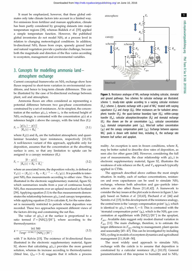
Figure 3. Resistance analogue of NH3 exchange including cuticular, stomataland ground pathways. Two schemes for cuticular exchange are illustrated:scheme 1, steady-state uptake according to a varying cuticular resistance(Rw); scheme 2, dynamic exchange with a pool of NH4

þ treated with varyingcapacitance (Cd) and charge (Qd). Other resistances are for turbulent atmos-pheric transfer (Ra), the quasi-laminar boundary layer (Rb), within-canopytransfer (Rac), cuticular adsorption/desorption (Rd) and stomatal exchange(Rs). Also shown are the air concentration (xa), cuticular concentration(xd), stomatal compensation point (xs), litter/soil surface concentration(xl) and the canopy compensation point (xc). Exchange between aqueousNH4þ pools is shown with dashed lines, including Kr, the exchange rate

between leaf surface and apoplast.

ilTransRSocB

368:20130166

3. Concepts for modelling ammonia land –atmosphere exchange

Current conceptual frameworks on NH3 exchange show how

fluxes respond to short-term variation in environmental con-

ditions, and hence to long-term climate differences. This can

be illustrated by the case of bi-directional exchange between

plant, soil and atmosphere.

Ammonia fluxes are often considered as representing a

potential difference between two gas-phase concentrations

constrained by a set of resistances. At its simplest, the concen-

tration at the surface x(zo0), where zo0 is the notional height of

NH3 exchange, is contrasted with the concentration x(z) at a

reference height z above the canopy, with the total flux (Ft):

Ft ¼½xðzo0 Þ � xðzÞ�½RaðzÞ þ Rb�

; ð3:1Þ

where Ra(z) and Rb are the turbulent atmospheric and quasi-

laminar boundary layer resistances, respectively [10,15].

A well-known variant of this approach, applicable only for

deposition, assumes that the concentration at the absorbing

surface is zero, so that any limitation to uptake can be

assigned to a canopy resistance (Rc):

Ft ¼½0� xðzÞ�

½RaðzÞ þ Rb þ Rc�; ð3:2Þ

where an associated term, the deposition velocity, is defined as

VdðzÞ ¼ ðRaðzÞ þ Rb þ RcÞ�1 ¼ �Ft=xðzÞ: It is possible to inter-

pret NH3 flux measurements according to either view. This is

illustrated in the electronic supplementary material, figure S2,

which summarizes results from a year of continuous hourly

NH3 flux measurements over an upland moorland in Scotland

[39]. Applying equation (3.1) to the flux measurements demon-

strates the relationship between x(zo0) and canopy temperature,

while applying equation (3.2) to calculate Rc for the same data-

set is necessarily restricted to periods where deposition was

recorded. These two approaches represent different views of

the factors driving and constraining the net flux.

The value of x(zo0) at the surface is proportional to a

ratio termed G ¼ [NH4þ]/[Hþ], where according to the

thermodynamics:

x ¼ 161 500

Texpð�10 380=TÞ½NHþ4 �=½Hþ�; ð3:3Þ

with T in Kelvin [15]. The existence of bi-directional fluxes

illustrated in the electronic supplementary material, figure

S2, shows that calculating x(zo0) provides the more general

solution, whereas its increase according to thermodynamics

(fitted line, Q10 ¼ 3–4) suggests that it reflects a process

reality. An exception is seen in frozen conditions, where Rc

may be better suited to describe slow rates of deposition, as

seen also for other gases [40]. However, considering the full

year of measurements, the clear relationship with x(zo0) in

electronic supplementary material, figure S2, illustrates the

weakness of sole reliance on the Rc and Vd approach typically

applied in CTMs.

The approach described above outlines the most simple

situation. In reality, each of surface concentrations, resistan-

ces and even capacitances can be used to simulate NH3

exchange, whereas both advection and gas–particle inter-

actions can also affect fluxes [11,41,42]. A framework to

consider the key issues at the plot scale is shown in figure 3, lar-

gely based on Sutton et al. [10,43], Flechard et al. [44] and

Nemitz et al. [15]. In this development of the resistance analogy,

the central term is the ‘canopy compensation point’ (xc), which

is identical to x(zo0) when Ft ¼ 0. This is contrasted with the

‘stomatal compensation point’ (xs), which is the NH3 gas con-

centration at equilibrium with [NH4þ]/[Hþ] in the apoplast,

Gapo. Available data suggest only modest diurnal variation in

Gapo [11]. The main challenge, therefore, is to estimate the

larger differences in Gapo owing to management, plant species

and seasonality [45–47]. This can be investigated by including

NH3 cycling in models of ecosystem dynamics and agricultural

management [11,18,48–50].

The most widely used approach to simulate NH3

exchange with the cuticle is to assume that deposition is

constrained by a cuticular resistance (Rw) [10,15]. General

parametrizations of this response to humidity and to NH3:

rstb.royalsocietypublishing.orgPhilTransR

SocB368:20130166

6

on June 10, 2016http://rstb.royalsocietypublishing.org/Downloaded from

acid-gas ratios have been developed ([15,46,51]; electronic

supplementary material, figure S3; figure 3, scheme 1).

These approaches have the advantage of relative simplicity,

but only represent a steady-state approximation to a dynamic

reality, where both adsorption (favouring net deposition) and

desorption (favouring emission) occur in practice.

This dynamic view can be addressed by scheme 2 of figure 3.

In the simplest description, a time-constant can be set for

charging and discharging the leaf-surface water/cuticular

pool of NHx (e.g. Rd ¼ 5000/Cd, s m21), combined with a

fixed leaf-surface pH [43]. A more sophisticated approach

solves the ion balance of the leaf-surface water, calculating

cuticular pH according to the concentrations, fluxes and precipi-

tation inputs of all relevant compounds [44,52]. In an extended

application to measurements over forest, Neirynck &

Ceulemans [53] tested the simpler application of scheme 2,

finding it to simulate duirnal to seasonal measured fluxes

much more closely than scheme 1. One of the main uncertain-

ties in applying scheme 2 is the exchange of aqueous NH4þ and

other ions between leaf surface and apoplast.

The last component of figure 3 describes NH3 exchange

with the ground surface. Although flux measurements have

often shown significant emission from soils and especially

with leaf litter [8,11,15], this term remains the most uncertain.

In particular, the extent to which soil pH influences pH at

atmospheric exchange surfaces such as leaf litter and in the

vicinity of applied fertilizer and manure remains poorly quan-

tified, while the liberation of NH3 from organic decomposition

directly influences local substrate pH. Further measurements

are needed to develop simple parametrizations of Gl for litter

and to inform the development of ecosystem models simulating

Gl in relation to litter quality, water availability, mineralization,

immobilization and nitrification rates.

Similar interactions apply to other NH3 volatilization

sources. For example, the VOLT’AIR model provides a process

simulation of NH3 emissions from the land application of

liquid manures [54,55], where manure placement method

and calculated soil infiltration rates inform the calculation of

x(zo0). Empirical approaches have also been used to parame-

trize NH3 emissions directly from manure application, using

regression with experimental studies [56]. Such empirical

relationships have also been applied to estimate NH3 emissions

from animal houses, manure stores and manure spreading (see

the electronic supplementary material, section S3). It remains a

future challenge to develop process models for these sources

based on the principles of equation (3.1).

4. Quantifying environmental relationships withammonia fluxes and concentrations

From the preceding examples it can be seen that temperature

and moisture play a key role in determining the concentra-

tion of NH3 in equilibrium with surface pools and hence

in defining net NH3 fluxes on diurnal to annual scales.

However, the interaction between these and other factors

(e.g. stomatal opening, growth dilution of NHx pools,

soil infiltration and decomposition rates) means that the

temperature-dependence of NH3 emission may not always

follow the thermodynamic response.

These interactions are illustrated in the electronic sup-

plementary material, figure S3b, which shows the values of

xc for periods when the net flux was zero, from NH3 flux

measurements over dry heathland [57]. Under very dry con-

ditions (relative humidity, h , 50%), cuticular fluxes appear

to have been small, so that xc � xs, with a clear temperature

dependence in the range of Q10 2–4. By contrast, at h in the

range 50–70%, there was less relationship to temperature,

pointing to a significant role of cuticular adsorption/

desorption processes.

The way in which plant growth interactions may alter the

temperature response of NH3 fluxes can be illustrated by the

process model PaSim. Based on its application to measured

fluxes over Scottish grassland [48], the model was used to

consider scenarios of altered annual air temperature, keeping

all other factors the same as the original simulation. The effect

of cutting and fertilization on the net NH3 flux and illustra-

tive Nr pools are shown in figure 4. PaSim included the

standard thermodynamic dependence of both xs and xsoil

(equation (3.3)) to simulated values of Gs and Gsoil (combined

with scheme 1 using Rw ¼ 30e(1002h)/7 s m21). It is, therefore,

notable that the net flux showed only a modest temperature-

dependence, with the net flux for the month increasing with

Q10 ¼ 1.5. Only immediately after fertilizer application did

the flux increase with Q10 ¼ 3.2. This can be explained by

the warmer temperatures leading to more rapid grass

growth, decreasing leaf substrate Nr and modelled Gs

(figure 4). Although further measurements have also shown

a role of leaf litter processes not currently treated in PaSim

[11], the simulation demonstrates how growth-related factors

can offset the simple thermodynamic NHx response.

A similar message emerges for NH3 emissions from land-

spreading of manures using the ALFAM multiple regression

model [56], which includes a weak temperature response

(Q10 ¼ 1.25). This broadly agrees with a simple empirical

approach for pig slurry for the UK ammonia inventory [27],

though, for cattle slurry, the distinction between summer

and other months in the inventory equates to Q10 ¼ 2.5. In

this case, the key interaction appears to be between volatiliz-

ation potential and slurry infiltration rate, which can be

limited in both waterlogged and hard–dry soils.

Atmospheric NH3 monitoring can also inform the simula-

tion of seasonal dynamics. In the case of the UK and Danish

ammonia networks, areas dominated by cattle and pig show

peak emissions in spring, which are reproduced by models

accounting for the timing of manure spreading [30,58]. How-

ever, the UK also includes substantial background areas (see

the electronic supplementary material, figure S1) with a

pronounced summer maximum and winter minimum of 0.43

and 0.04 mg NH3 m23, respectively, while sheep-dominated

upland areas show a similar annual cycle (0.95 and

0.17 mg m23, respectively). These seasonal patterns are not

reproduced in CTMs as they do not adequately treat the climatic

dependence of grazing emissions [58]. As the grazing animals

that dominate emissions in these areas are outdoors all year, a

128C difference between the mean temperature of warmest

and coolest month equates to a Q10 of 9.0 and 4.7 for background

and sheep sites, respectively. These large values suggest that

other factors enhance the temperature-dependence of NH3

concentrations, with more rapid scavenging in winter.

Such seasonal differences can also be seen from globally

monitored satellite columns of NH3 at 12� 12 km2 resolution

at nadir, through processing of retrievals from the infrared

atmospheric sounding interferometer on the MetOp platform.

This approach is based on the absorption spectra of NH3 in

the infrared and depends on a strong thermal contrast between

0.007(a)

(b)

40000

G s= [N

H4+) s/

[H+] s

30000

20000

10000

0

Nsubs T(–3)Nsubs T(0)

Nsubs T(+3)gamma T(0)gamma T(–3)

gamma T(+3)

0.006

0.005

0.004

0.003

0.002

1000

flux T(0)

flux T(+3)

flux T(–3)

gras

s cu

t

fert

ilize

r

NH

3 fl

ux to

tal (

ng m

–2 s–1

)su

bstr

ate

nitr

ogen

(kg

N p

er k

g D

M)

800

600

400

200

24 July 28 July 01 August 05 August 09 August 13 August 17 August 21 August0

–200Figure 4. Effect of temperature scenarios (annual change of þ38C and 238C) on (a) simulated nitrogen pools ( foliar substrate N, and Gs) and (b) net NH3 fluxes.Simulations conducted using the PaSim model for managed grassland in Scotland following cutting and fertilization with ammonium nitrate.

rstb.royalsocietypublishing.orgPhilTransR

SocB368:20130166

7

on June 10, 2016http://rstb.royalsocietypublishing.org/Downloaded from

the ground and atmosphere, measuring NH3 columns that are

dominated by high concentrations in the lowest 1–2 km [37].

Retrievals are made twice a day, allowing extensive comparison

with environmental and seasonal NH3 dynamics.

An illustration of the satellite retrieval is shown in figure 5,

which compares the mean NH3 column over Europe with the

seasonally varying NH3 column at three sites where ground-

based monitoring of NH3 concentrations is available. The

map distinguishes areas of high agricultural NH3 emissions

in Brittany, E England, the Netherlands and NW Germany,

Po Valley and Nile Delta, while showing high values across

Belarus and SW Russia related to forest fires during 2010.

The magnitude of the NH3 columns are also a function of

spatial differences in atmospheric mixing that might explain

why smaller values are seen in the west compared with the

east of the UK. For Stoke Ferry, where NH3 emissions are domi-

nated by pig and poultry (see the electronic supplementary

material, figure S1), both the ground-based and satellite data

show spring peak NH3 values, associated with land-spreading

of manure. At Vredepeel, an area of intense pig and cattle farm-

ing in the Netherlands, there is less seasonality in the NH3 data,

indicating a stronger contribution of controlled environment

livestock housing. Lastly, at K-Puszta, a Hungarian site more

distant from local sources, NH3 levels are highest in summer

and lowest in winter, reflecting the integration of different

environmentally dependent sources.

The satellite approach requires a strong thermal contrast,

limiting its capability in winter and cloudy conditions. How-

ever, it allows the examination of spatial patterns and

temporal trends with a global coverage that could never be

achieved by ground-based air sampling. It thus provides an

unprecedented opportunity to improve our understanding

of the sources, management and climate controls on NH3,

as further illustrated by seasonal NH3 patterns in different

parts of the world. In the case of the Po Valley, Nile Delta,

California and Pakistan, there is a strong seasonal cycle in

NH3, with values of Q10 of the column totals mostly in the

range 2–3. However, not all locations show such a tempera-

ture-dependence, especially where management differences

drive seasonality in NH3 emissions as seen in livestock

dominated areas of Belgium and China (see the electronic

supplementary material, figure S4). In order to derive the maxi-

mum value from the satellite data, these, therefore, need to be

interpreted using detailed atmospheric models, as a basis to

disentangle the different driving factors.

5. Seabirds as a model system to assess climate-dependence of global ammonia emissions

The preceding examples highlight the many factors controlling

NH3 emissions, including management effects. In the case of

monitoring NH3 concentrations and atmospheric columns,

an even larger number of meteorological factors affect

observed values. For these reasons, there is a strong case to

use model ecosystems to assess the climate-dependence of

NH3 exchange. At present, this can uniquely be demonstrated

by the case of NH3 emissions from seabird colonies, building

on recent measurements and modelling [35,59].

Seabird colonies provide several advantages as a ‘model

system’ to investigate the climate-dependence of NH3 emissions:

the birds follow a well-established annual breeding cycle little

affected by human management; rates of Nr excretion can be

directly related to dietary energetics for well-characterized

populations; and they typically form locally strong NH3 sources

in areas of low NH3 background. Riddick et al. [35] estimated

global NH3 emission from seabird colonies at 0.3 (0.1–

0.4) Tg yr21. Although this is a small fraction of total emissions,

it includes major point/island sources greater than

15 Gg NH3 yr21, with sites distributed globally across a wide

range of climates.

Colony-scale NH3 flux measurements from seabird colo-

nies were first reported by Blackall et al. [59] for Scottish

islands, and these have been extended for contrasting climates

3.5

NH3 1016 molecules per cm–2

300

300

285

270

T (

K)

colu

mn

[NH

3]

T (

K)

colu

mn

(NH

3)

2.0

4.0

3.0

1.0

0

300

290

270

280

T (

K)

colu

mn

[NH

3]

1.6

0.8

0

8

6

4

2

surf

ace

[NH

3] (

µg m

–3)

surf

ace

[NH

3] (

µg m

–3)

0

0

10

20

30

40

surf

ace

[NH

3] (

µg m

–3)

0

1

2

3

4

Stoke Ferry

Vredepeel

K-Puszta

2009 2010 2011 2012

2009 2010 2011 2012

2009 2010 2011 2012

1.5

1.0

290

280

2703.2

2.9

2.6

2.3

2.0

1.7

1.4

1.1

0.80

0.50

Figure 5. Satellite estimates of the NH3 column (106 molecules cm22) and ground temperature, showing the mean for 2009, 2010 and 2011 (from the infraredatmospheric sounding interferometer on the MetOp platform), as compared with ground-based measurements of atmospheric NH3 concentrations at threeselected sites.

rstb.royalsocietypublishing.orgPhilTransR

SocB368:20130166

8

on June 10, 2016http://rstb.royalsocietypublishing.org/Downloaded from

as illustrated in figure 6. In this graph, measured NH3 emis-

sions have been normalized by calculated Nr excretion rates

to show the percentage of Nr that is volatilized (Pv). The

measurements show a clear temperature-dependence across

the globe, with Q10 � 3. For comparison, the dotted line is

the estimate used by Blackall et al. [59] for global upscaling,

whereas the solid line is the initial temperature-adjusted

upscaling of Riddick et al. [35], following equation (3.3) (their

scenario 2).

The importance of these measurements is emphasized by

their use to verify a process-based model of NH3 emissions,

the GUANO model (see the electronic supplementary material,

figure S5). The model is driven by excretal inputs according to

bird diet, energetics and numbers combined with a water-bal-

ance to estimate liquid-phase Nr concentrations and run-off.

Hydrolysis of uric acid to ammoniacal nitrogen is moisture-

and temperature-dependent. By combining the modelled

value of [NH4þ] with a guano pH of 8.5 and ground surface

temperature, equation (3.3) allows estimation of x(zo0). This is

then applied in equation (3.1) to calculate hourly NH3 emission.

Application of the GUANO model shows close agreement

with measurements, the hourly NH3 fluxes responding to

fluctuations in surface temperature, precipitation events and

wind speed. The overall measured temperature-dependence

is also reproduced by the GUANO model (figure 6),

including a difference between the two warmest sites, Michel-

mas Cay and Ascension Island. This is explained by the latter

being very dry, limiting rates of uric acid hydrolysis, and

hence both measured and modelled NH3 emission.

Based on the verification of the GUANO model with field

measurements, the global seabird and excretion datasets [35]

have been applied in the model for hourly simulation of 9000

colonies for 2010–2011 (figure 7). Ground temperature turns

out to be the primary driver globally, with Pv ranging from

20 to 72 per cent for sites with annual mean temperature of

308C, whereas for sites with a mean temperature of 08C, Pv

was 0–18%. Variation between sites of similar temperatures

is mainly attributable to differences in water availability,

wind speed and nesting habitat (e.g. bare rock versus

burrow breeders).

6. Climate-dependent assessment of ammoniaemissions, transport and deposition

The examples presented for terrestrial systems including grass-

land, shrubland, forest and seabird colonies demonstrate the

clear climatic dependence of NH3 exchange processes. Agricul-

tural systems are more complex, and include interactions with

management (including alteration of management timing and

10

20

30

40

50

60

70

80

90

100

average temperature during measurements (°C)

perc

enta

ge N

vol

atili

zed

as N

H3

(Pv,

%)

whole island,Isle of May,

Scotland (2004)

Michaelmas Cay,Australia

Signy Island,South Orkney

Big Mac, Bird Island

0 5 10 15 20 25 30 35

GUANO model

measurements [59]

measurements [35]

Bass Rock,Scotland (2004)

Ascension Island,South Atlantic

Puffin Colony, Isle ofMay, Scotland (2009)

Figure 6. Measured percentage of excreted Nr that is volatilized as NH3 (Pv) as a function of mean temperature during field campaigns (dashed line: Pv(%) ¼1.9354e0.109 T; R2 ¼ 0.75), as compared with estimates from the GUANO model for a global selection of seabird colonies. The dotted line shows the value used in afirst bioeneregics (BE) model of Blackall et al. [59], while the solid line was applied in a temperature-adjusted bioenergetics (TABE) model, by Riddick et al. [35]using equation (3.3). The bars on the measured points apply to colonies including burrow-nesting birds and indicate the estimated Pv if the colony were entirelypopulated by bare-rock breeders.

180° W 160° W 140° W 120° W 100° W 80° W 60° W 40° W 20° W 0° 20° E 40° E 60° E 80° E 100° E 120° E 140° E 160° E

80° N

60° N

40° N

20° N

20° S

60° S60° S

40° S

20° S

0°

average PV (%)

0–5

6–15

16–30

31–45

46–100

20° N

Pacific Ocean

Atlantic Ocean

Indian Ocean

Pacific Ocean

40° N

60° N

80° N

80° S80° S

0° N

180°

180° 160° W 140° W 120° W100° W 80° W 60° W 40° W 20° W 0° 20° E 40° E 60° E 80° E 100° E 120° E 140° E 160° E 180°

Figure 7. Global application of the GUANO model illustrating the average percentage of excreted N that is volatilized as NH3. Excretion calculated based on colonyseabird energetics [35], combined with hourly meteorological estimates through 2010 – 2011.

rstb.royalsocietypublishing.orgPhilTransR

SocB368:20130166

9

on June 10, 2016http://rstb.royalsocietypublishing.org/Downloaded from

systems), Nr type, animal housing and manure application

method. In principle, however, many of the climatic inter-

actions apply, and can be addressed using process-based

models. The same is true for ocean–atmosphere NH3

exchange, which is bi-directional according to equation (3.1),

with x(zo0) depending on variations in sea surface temperature,

[NH4þ] concentration, water pH and local NH3 air concen-

trations. For example, future ocean acidification would tend

to decrease sea-surface NH3 emission. Of these factors, Johnson

et al. [60] found temperature to be of overriding importance in

determining ocean NH3 emissions, through its control of x(zo0).

With this background, we return to the question of regional

and global modelling of NH3 emission, dispersion and depo-

sition in CTMs. Section 2 showed that there are several

limitations in current NH3 emission inventories, such as infor-

mation on activity data (numbers and location of animals,

fertilizers, fires, etc.), average emission rates and data structure

(distinction of source sectors). On a global scale, however,

and given the target to assess climate change effects, by far

the main limitation is that current architecture uses previously

calculated emissions as input to CTMs. In reality, the same

meteorology incorporated within a CTM to describe chemical

chemistry andtransportmodule

uni-directionalemission

module (point)

meteorologicalmodel

climate modelGCM/RCM

hourlyemissions

bi-directionalexchange

module (area)

verification (and assimilation)

meteo data(T, ?, …)

farm and otherstatistics

climatedrivers

activity data

by sub-sector

land use andland cover

experimentalemission

relationships

earth observationand ground-based

measurements

hourly air concs. andbi-directional fluxes

Figure 8. Proposed modelling architecture for treating the climate-dependence of ammonia fluxes in regional and global atmospheric transport and chemistrymodels. In this approach, static emission inventories are replaced by calculations depending on prevailing meteorology, while allowing for bi-directional exchangewith area sources/sinks, giving the basis to assess climate change scenarios including the consequences of climate feedbacks through altered NH3 emissions. Theeffect of altered air chemistry may also be fed back into the climate model.

rstb.royalsocietypublishing.orgPhilTransR

SocB368:20130166

10

on June 10, 2016http://rstb.royalsocietypublishing.org/Downloaded from

transport and transformation will have a major effect on short-

and long-term control of NH3 emissions, deposition and bi-

directional exchange. For example, on a warm sunny day,

emissions from manure, fertilizers and plants will be at their

maximum, whereas cuticular deposition of NH3 will be at its

minimum, with the same conditions promoting thermal con-

vection in the atmospheric boundary layer, increasing the

atmospheric transport distance.

To address the coupling of these processes requires a new

paradigm for atmospheric NH3 modelling. For this purpose,

the long-term goal must be to replace the use of previously

determined emission inventories with a suite of spatial

activity databases and models that allow emissions to be cal-

culated online as part of the running of the CTMs. Such an

approach is already widely adopted for biogenic hydro-

carbon emissions from vegetation [20]. In this way, both the

environmental dependence of uni-directional NH3 emissions

and of bi-directional NH3 fluxes become incorporated into

the overall model. In the case of the bi-directional part,

online calculation is essential because of the feedback

between x(z) and the direction/magnitude of the net flux.

An outline of the proposed modelling architecture is given in

figure 8, with the key new elements highlighted in green. Instead

of activity data and experimentally derived relationships being

used directly to provide an ‘emissions inventory’, with sub-

sequent (uni-directional) dry deposition, emissions are treated

in two submodels: (i) uni-directional emissions from point

sources such as manure storage facilities and animal housing

(where x(zo0)� x(z)) and (ii) bi-directional fluxes from area

sources (where x(zo0) is less than or greater than x(z)), which

includes emissions or dry deposition according to prevailing

conditions. The same meteorological data are thus used to

drive the emissions, chemistry transport and bi-directional

exchange. With this structure, climatic differences between

locations are incorporated, while climate change scenarios can

be directly applied.

At the present time, many of the elements for a new archi-

tecture are already available to build such a system at regional

and global scales. Emission models such as those for animal

houses and manure spreading [54,55] need to be linked to

CTMs incorporating bi-directional exchange parametrizations.

Simple process models, following the principles used in the

GUANO model, should be further developed and their scope

extended. While the most detailed dynamic model of bi-direc-

tional canopy exchange [44] has many input uncertainties, the

analysis of Neirynck & Ceulemans [53] suggests that a move

from scheme 1 towards the simpler application of scheme 2

should be a feasible future target. These developments will

require further information to parametrize G for ecosystem

components, while upscaling models must include infor-

mation on canopy and ground temperature, surface wetness

and relative humidity and soil pH. While many of the necess-

ary terms are available from meteorological models, a

coupling with agricultural and ecosystem models becomes

increasingly important for detailed simulation of

the interactions. Challenges related to subgrid variability are

addressed in the electronic supplementary material, S7.

Although not all these linkages have yet been made, signifi-

cant progress in the temporal distribution of NH3 emissions

according to agricultural activities has already been achieved,

which can provide key input to the future developments

[30,61,62]. For example, the US EPA Community Multiscale

Air-Quality model includes coupling to an agro-ecosystem

model to provide dynamic and meteorological-dependent

rstb.royalsocietypublishing.orgPhilTransR

SocB36

11

on June 10, 2016http://rstb.royalsocietypublishing.org/Downloaded from

emissions from fertilizer application, using a two-layer bidirec-

tional resistance model based on Nemitz et al. [15] that

includes the effects of soil nitrification processes [18]. Similarly,

Hamaoui-Lagel et al. [55] incorporated the VOLT’AIR model to

simulate NH3 emissions from fertilizer application in a regional-

scale atmospheric model.

The consequences of such temporal interactions can be

illustrated by the comparison of measured NH3 concentra-

tion and simulations of a Danish model [22] at a long-term

monitoring site (Tange, electronic supplementary material,

figure S6). In this case, the model has been used to provide

the temporal disaggregation of previously calculated annual

emissions. The challenge for the next stage must be to incor-

porate the environmental drivers in process models for all

major sources to quantify the dynamics on hourly, diurnal,

seasonal and annual scales, and as a foundation to estimate

the effects of long-term climate change.

8:20130166

7. ConclusionsThis paper has shown how ammonia emissions and deposition

are fundamentally dependent on environmental conditions.

While temperature has been found to be the primary environ-

mental driver, other key factors include interactions with

canopy and soil wetness and with management practices for

agricultural sources. For several systems, such as emission

from manure spreading, fertilizers, seabird colonies and

bidirectional exchange with vegetation, process models are

already available that describe the key relationships.

A new paradigm for atmospheric modelling of NH3 is pro-

posed, where process models are incorporated with the

relevant statistical data to simulate NH3 emissions as part of

atmospheric models. Seabird colonies have been used here to

demonstrate the global application of such a process model,

verified by measurements under different climates, where

the fraction of available Nr volatilized as NH3 can increase

by a factor of more than 20 between subpolar and tropical

conditions. Although a few CTMs have incorporated bidirec-

tional exchange, work is required to parametrize models for

different ecosystem types and climates, and to assess the con-

sequences of different levels of model complexity, including

the coupling with ecosystem and agronomic models.

The proposed developments provide the necessary foun-

dation to assess how climate will affect NH3 emissions,

dispersion and deposition. The practical implications are that

inventory activities should focus increasingly on supplying

the statistical activity data needed to drive the models (rather

than only publishing static NH3 emission estimates) and that

national NH3 emissions for any year can only be calculated

with confidence once the meteorological data are available.

Based on the available measurements and models, it is poss-

ible to indicate empirically the scale of the climate risk for NH3.

Marine NH3 emissions are expected to follow the thermodyn-

amic response directly (equation (3.3)), whereas a reduced Q10

of 2 (1.5–3) may be applied for terrestrial volatilization sources.

(For procedures, see the electronic supplementary material,

section 8, figures S7, S8 and equations for use in scenario

models.) Applying these responses to the 2008 global estimates

of 65 (46–85) Tg N yr21 for a 58C global temperature increase

to 2100 would increase NH3 emissions by approximately 42

per cent (28–67%) to 93 (64–125) Tg. If this is combined with

a further 56 per cent (44–67%) increase in anthropogenic

source activities [63,64], total NH3 emissions would reach 132

(89–179) Tg by 2100. Considering these major anticipated

increases, the limited progress in NH3 mitigation efforts to

date, and the slow nature of behavioural change, stepping up

efforts to control NH3 emission must be a key priority for

future policy development.

Full acknowledgements, including from the European Commission,European Space Agency, US EPA, other national funding sources andindividuals are listed in the electronic supplementary material. Thispaper is a contribution to the International Nitrogen Initiative (INI)and to the UNECE Task Force on Reactive Nitrogen (UNECE).

References

1. Erisman JW, Sutton MA, Galloway JN, Klimont Z,Winiwarter W. 2008 How a century of ammoniasynthesis changed the world. Nat. Geosci. 1, 636 –639. (doi:10.1038/ngeo325)

2. Sutton MA, Erisman JW, Dentener F, Moller D. 2008Ammonia in the environment: from ancient timesto the present. Environ. Pollut. 156, 583 – 604.(doi:10.1016/j.envpol.2008.03.013)

3. CEIP. 2012 Overview of submissions under CLRTAP:2012. Vienna, Austria: Centre for EmissionsInventories and Projections, Umweltbundesamt(www.ceip.at/overview-of-submissions-under-clrtap/2012-submissions/)

4. UNECE. 2012 Draft decision on amending the text ofand annexes II to IX to the Gothenburg protocol toabate acidification, eutrophication and ground-levelozone and addition of new annexes X and XI.Geneva, Switzerland: Executive Body for theConvention on Long-range Transboundary AirPollution.

5. Pinder RW, Gilliland AB, Dennis RL. 2008Environmental impact of atmospheric NH3 emissionsunder present and future conditions in the easternUnited States. Geophys. Res. Letts. 35, L12808.(doi:10.1029/2008GL033732)

6. Sutton MA et al. 2011 Summary for policy makers.In The European nitrogen assessment (eds MASutton, CM Howard, JW Erisman, G Billen,A Bleeker, P Grennfelt, H van Grinsven, B Grizzetti),pp. xxiv – xxxiv. Cambridge, UK: CambridgeUniversity Press.

7. Sutton MA, Oenema O, Erisman JW, Leip A, vanGrinsven H, Winiwarter W. 2011 Too much of a goodthing. Nature 472, 159 – 161. (doi:10.1038/472159a)

8. Denmead OT, Freney JR, Simpson JR. 1976 A closedammonia cycle within a plant canopy. Soil Sci.Biochem. 8, 161 – 164. (doi:10.1016/0038-0717(76)90083-3)

9. Farquhar GD, Firth PM, Wetselaar R, Wier B. 1980On the gaseous exchange of ammonia between

leaves and the environment: determination of theammonia compensation point. Plant Physiol. 66,710 – 714. (doi:10.1104/pp.66.4.710)

10. Sutton MA, Schjorring JK, Wyers GP. 1995 Plantatmosphere exchange of ammonia. Phil.Trans. R. Soc. A 351, 261 – 276. (doi:10.1098/rsta.1995.0033)

11. Sutton MA et al. 2009 Dynamics of ammoniaexchange with cut grassland: synthesis of resultsand conclusions of the GRAMINAE integratedexperiment. Biogeosciences 6, 2907 – 2934. (doi:10.5194/bg-6-2907-2009)

12. Sutton MA, Reis S, Baker SMH (eds). 2009Atmospheric ammonia: detecting emission changesand environmental impacts, p. 464. Berlin, Germany:Springer.

13. Schjoerring JK, Husted S, Mattsson M. 1998Physiological parameters controlling plant –atmosphere ammonia exchange. Atmos. Environ. 32,491 – 498. (doi:10.1016/S1352-2310(97)00006-X)

rstb.royalsocietypublishing.orgPhilTransR

SocB368:20130166

12

on June 10, 2016http://rstb.royalsocietypublishing.org/Downloaded from

14. Hertel O et al. 2011 Nitrogen processes in theatmosphere. In The European nitrogen assessment(eds MA Sutton, CM Howard, JW Erisman, G Billen,A Bleeker, P Grennfelt, H van Grinsven, B Grizzetti),Ch. 9, pp. 177 – 207. Cambridge, UK: CambridgeUniversity Press.

15. Nemitz E, Milford C, Sutton MA. 2001 A two-layercanopy compensation point model for describing bi-directional biosphere/atmosphere exchange ofammonia. Q. J. Roy. Meteor. Soc. 127, 815 – 833.(doi:10.1256/smsqj.57305)

16. Dentener FJ, Crutzen PJ. 1994 A three-dimensionalmodel of the global ammonia cycle. J. Atmos.Chem. 19, 331 – 369. (doi:10.1007/BF00694492)

17. Wichink Kruit RJ, Schaap M, Sauter FJ, Van ZantenMC, van Pul WAJ. 2012 Modeling the distribution ofammonia across Europe including bi-directionalsurface-atmosphere exchange. Biogeosciences 9,5261 – 5277. (doi:10.5194/bg-9-5261-2012)

18. Bash JO, Cooter EJ, Dennis RL, Walker JT, Pleim JE.2012 Evaluation of a regional air-quality modelwith bi-directional NH3 exchange coupled to anagro-ecosystem model. Biogeosciences 10, 1635 –1645. (doi:10.5194/bg-10-1635-2013)

19. Cape JN, van der Eerden LJ, Sheppard LJ,Leith ID, Sutton MA. 2009 Evidence forchanging the critical level for ammonia.Environ. Pollut. 157, 1033 – 1037. (doi:10.1016/j.envpol.2008.09.049)

20. Simpson D et al. 2011 Atmospheric transport anddeposition of reactive nitrogen in Europe. In TheEuropean nitrogen assessment (eds MA Sutton,CM Howard, JW Erisman, G Billen, A Bleeker,P Grennfelt, H van Grinsven, B Grizzetti), ch. 14,pp. 298 – 316. Cambridge, UK: Cambridge UniversityPress.

21. Velthof VGL, van Bruggen C, Groenestein CM,de Haan BJ, Hoogeveen MW, Huijsmans JFM. 2012A model for inventory of ammonia emissions fromagriculture in the Netherlands. Atmos. Environ. 46,248 – 255. (doi:10.1016/j.atmosenv.2011.09.075)

22. Geels C et al. 2012 A coupled model system(DAMOS) improves the accuracy of simulatedatmospheric ammonia levels over Denmark.Biogeosciences 9, 2625 – 2647. (doi:10.5194/bg-9-2625-2012)

23. Dragosits U, Sutton MA, Place CJ, Bayley A. 1998Modelling the spatial distribution of ammoniaemissions in the UK. Environ. Pollut. 102, 195 – 203.(doi:10.1016/S0269-7491(98)80033-X)

24. Webb J, Misselbrook TH. 2004 A mass-flow modelof ammonia emissions from UK livestock production.Atmos. Environ. 38, 2163 – 2176. (doi:10.1016/j.atmosenv.2004.01.023)

25. de Vries W, Leip A, Reinds GJ, Kros J, Lesschen JP,Bouwman AF. 2011 Comparison of land nitrogenbudgets for European agriculture by variousmodeling approaches. Environ. Pollut. 159,3254 – 3268. (doi:10.1016/j.envpol.2011.03.038)

26. Bleeker A et al. 2009 Linking ammonia emissiontrends to measured concentrations and depositionof reduced nitrogen at different scales. InAtmospheric ammonia: detecting emission changes

and environmental impacts (eds MA Sutton, S Reis,SMH Baker), pp. 123 – 180. Berlin, Germany:Springer.

27. Misselbrook TH, Sutton MA, Scholefield D. 2004 Asimple process-based model for estimatingammonia emissions from agricultural land afterfertilizer applications. Soil Use Manag. 20,365 – 372. (doi:10.1079/SUM2004280)

28. Gross A, Boyd CE, Wood CW. 1999 Ammoniavolatilization from freshwater fish ponds. J. Environ.Qual. 28, 793 – 797. (doi:10.2134/jeq1999.00472425002800030009x)

29. Sutton MA, Dragosits U, Tang YS, Fowler D. 2000Ammonia emissions from non-agricultural sourcesin the UK. Atmos. Environ. 34, 855 – 869. (doi:10.1016/S1352-2310(99)00362-3)

30. Skjøth CA et al. 2011 Spatial and temporalvariations in ammonia emissions: a freely accessiblemodel code for Europe. Atmos. Chem. Phys. 11,5221 – 5236. (doi:10.5194/acp-11-5221-2011)

31. Bouwman AF, Lee DS, Asman WAH, Dentener FJ,Van der Hoek KW, Olivier JGJ. 1997 A global high-resolution emission inventory for ammonia. Glob.Biogeochem. Cycles 11, 561 – 587. (doi:10.1029/97GB02266)

32. Van Aardenne JA, Dentener FJ, Olivier JGJ, KleinGoldewijk CGM, Lelieveld J. 2001 A 18 � 18resolution data set of historical anthropogenic tracegas emissions for the period 1890 – 1990. Glob.Biogeochem. Cycles 15, 909 – 928. (doi:10.1029/2000GB001265)

33. Beusen AHW, Bouwman AF, Heuberger PSC, vanDrecht G, an Der Hoek KW. 2008 Bottom-upuncertainty estimates of global ammonia emissionsfrom global agricultural production systems. Atmos.Environ. 42, 6067 – 6077. (doi:10.1016/j.atmosenv.2008.03.044)

34. JRC/PBL. 2011 Emission database for globalatmospheric research, EDGAR v. 4.2. See http://edgar.jrc.ec.europa.eu/.

35. Riddick SN, Dragosits U, Blackall TD, Daunt F,Wanless S, Sutton MA. 2012 The global distributionof ammonia emissions from seabird colonies.Atmos. Environ. 55, 319 – 327. (doi:10.1016/j.atmosenv.2012.02.052)

36. Andres RJ, Kasgnoc AD. 1998 A time-averagedinventory of subaerial volcanic sulfur emissions.J. Geophys. Res. 103, 25 251 – 25 261. (doi:10.1029/98JD02091)

37. Clarisse L, Clerbaux C, Dentener F, Hurtmans D,Coheur PF. 2009 Global ammonia distributionderived from infrared satellite observations. Nat.Geosci. 2, 479 – 483. (doi:10.1038/ngeo551)

38. Bouwman AF, Boumans LJM, Batjes NH. 2002Estimation of global NH3 volatilization loss fromsynthetic fertilizers and animal manure applied toarable lands and grasslands. Glob. Biogeochem.Cycles 16, 1024. (doi:10.1029/2000GB001389)

39. Flechard CR, Fowler D. 1998 Atmospheric ammoniaat a moorland site. I. The meteorological control ofambient ammonia concentrations and the influenceof local sources. Q. J. Roy. Meteor. Soc. 124,733 – 757. (doi:10.1002/qj.49712454705)

40. Fowler D et al. 2009 Atmospheric compositionchange: ecosystems: atmosphere interactions.Atmos. Environ. 43, 5193 – 5267. (doi:10.1016/j.atmosenv.2009.07.068)

41. Nemitz E, Sutton MA. 2004 Gas-particle interactionsabove a Dutch heathland. III. Modelling the influenceof the NH3 – HNO3 – NH4NO3 equilibrium on size-segregated particle fluxes. Atmos. Chem. Phys. 4,1025 – 1045. (doi:10.5194/acp-4-1025-2004)

42. Loubet B et al. 2009 Ammonia deposition near hotspots: processes, models and monitoring methods. InAtmospheric ammonia: detecting emission changes andenvironmental impacts (eds MA Sutton, S Reis, SMHBaker), pp. 205 – 267. Berlin, Germany: Springer.

43. Sutton MA, Burkhardt JK, Guerin D, Nemitz E,Fowler D. 1998 Development of resistance modelsto describe measurements of bi-directionalammonia surface atmosphere exchange. Atmos.Environ. 32, 473 – 480. (doi:10.1016/S1352-2310(97)00164-7)

44. Flechard C, Fowler D, Sutton MA, Cape JN. 1999 Adynamic chemical model of bi-directional ammoniaexchange between semi-natural vegetation andthe atmosphere. Q. J. Roy. Meteor. Soc. 125,2611 – 2641. (doi:10.1002/qj.49712555914)

45. Mattsson M et al. 2009 Temporal variability inbioassays of the stomatal ammonia compensationpoint in relation to plant and soil nitrogenparameters in intensively managed grassland.Biogeosciences 6, 171 – 179. (doi:10.5194/bg-6-171-2009)

46. Massad R-S, Nemitz E, Sutton MA. 2010 Review andparameterisation of bi-directional ammoniaexchange between vegetation and the atmosphere.Atmos. Chem. Phys. 10, 10 359 – 10 386. (doi:10.5194/acp-10-10359-2010)

47. Wichink Kruit RJ, van Pul WAJ, Sauter FJ,van den Broek M, Nemitz E, Sutton MA, Krol M,Holtslag AAM. 2010 Modeling the surface-atmosphere exchange of ammonia. Atmos.Environ. 44, 945 – 957. (doi:10.1016/j.atmosenv.2009.11.049)

48. Riedo M, Milford C, Schmid M, Sutton MA. 2002Coupling soil – plant – atmosphere exchange ofammonia with ecosystem functioning in grasslands.Ecol. Model. 158, 83 – 110. (doi:10.1016/S0304-3800(02)00169-2)

49. Wu YH, Walker J, Schwede D, Peters-Lidard C,Dennis R, Robarge W. 2009 A new model of bi-directional ammonia exchange between theatmosphere and biosphere: ammonia stomatalcompensation point. Agr. Forest Meteorol. 149,263 – 280. (doi:10.1016/j.agrformet.2008.08.012)

50. Massad R-S, Tuzet A, Loubet B, Perrier A, Cellier P.2010 Model of stomatal ammonia compensationpoint (STAMP) in relation to the plant nitrogen andcarbon metabolisms and environmental conditions.Ecol. Model. 221, 479 – 494. (doi:10.1016/j.ecolmodel.2009.10.029)

51. Zhang L, Wright PL, Asman WAH. 2010 Bi-directional airsurface exchange of atmosphericammonia: a review of measurements and adevelopment of a big-leaf model for applications in

rstb.royalsocietypublishing.orgPhilTransR

SocB368:201301

13

on June 10, 2016http://rstb.royalsocietypublishing.org/Downloaded from

regional-scale air-quality models. J. Geophys. Res.115, D20310. (doi:10.1029/2009JD013589)

52. Burkhardt J et al. 2009 Modelling the dynamicchemical interactions of atmospheric ammonia withleaf surface wetness in a managed grasslandcanopy. Biogeosciences 6, 67 – 84. (doi:10.5194/bg-6-67-2009)

53. Neirynck J, Ceulemans R. 2008 Bidirectionalammonia exchange above a mixed coniferous forest.Environ. Pollut. 154, 424 – 438. (doi:10.1016/j.envpol.2007.11.030)

54. Genermont S, Cellier P. 1997 A mechanistic modelfor estimating ammonia volatilization from slurryapplied to bare soil. Agr. Forest Meteorol. 88,145 – 167. (doi:10.1016/S0168-1923(97)00044-0)

55. Hamaoui-Laguel L, Meleux F, Beekmann M,Bessagnet B, Genermont S, Cellier P, Letinois L.2012 Improving ammonia emissions in air qualitymodelling for France. Atmos. Environ. (doi:10.1016/j.atmosenv.2012.08.002)

56. Søgaard HT, Sommer SG, Hutchings NJ, HuijsmansJFM, Bussink DW, Nicholson F. 2002 Ammoniavolatilization from field-applied animal slurry—theALFAM model. Atmos. Environ. 36, 3309 – 3319.(doi:10.1016/S1352-2310(02)00300-X)

57. Nemitz E, Sutton MA, Wyers GP, Jongejan PAC. 2004Gas – particle interactions above a Dutch heathland.I. Surface exchange fluxes of NH3, SO2, HNO3 andHCl. Atmos. Chem. Phys. 4, 989 – 1005. (doi:10.5194/acp-4-989-2004)

58. Hellsten S, Dragosits U, Place CJ, Misselbrook TH, TangYS, Sutton MA. 2007 Modelling seasonal dynamicsfrom temporal variation in agricultural practices in theUK ammonia emission inventory. Water Air Soil Pollut.Focus 7, 3 – 13. (doi:10.1007/s11267-006-9087-5)

59. Blackall TD et al. 2007 Ammonia emissions fromseabird colonies. Geophys. Res. Lett. 34, L10801.(doi:10.1029/2006GL028928)

60. Johnson MT et al. 2008 Field observations of theocean – atmosphere exchange of ammonia:

fundamental importance of temperature as revealedby a comparison of high and low latitudes. Glob.Biogeochem. Cycles 22, GB1019. (doi:10.1029/2007GB003039)

61. Gilliland AB, Appel KW, Pinder RW, Dennis RL. 2006Seasonal NH3 emissions for the continental UnitedStates: inverse model estimation and evaluation.Atmos. Environ. 40, 4986 – 4998. (doi:10.1016/j.atmonsenv.2005.12.066)

62. Skjoth CA, Geels C. 2013 The effect of climate andclimate change on ammonia emissions in Europe.Atmos. 13, 117 – 128. (doi:10.5194/acp-13-117-2013)

63. Fowler D, Pyle JA, Raven JA, Sutton MA 2013 Theglobal nitrogen cycle in the twenty-first century:introduction. Phil. Trans. R. Soc. B 368, 20130165.(doi:10.1098/rstb.2013.0165)

64. Fowler D et al. 2013 The global nitrogen cycle inthe twenty-first century. Phil. Trans. R. Soc. B 368,20130164. (doi:10.1098/rstb.2013.0164)

6

6