Towards a Multiscale Scheme for Nonlinear Dynamic Analysis ... · Towards a Multiscale Scheme for...

Towards a Multiscale Schemefor Nonlinear Dynamic Analysisof Masonry Structures with Damage

Savvas P. Triantafyllou and Eleni N. Chatzi

Abstract In this work, a three dimensional multiscale formulation is presented forthe analysis of masonry structures based on the multiscale finite element formu-lation. The method is developed within the framework of the Enhanced MultiscaleFinite Element Method. Through this approach, two discretization schemes areconsidered, namely a fine mesh that accounts for the micro-structure and a coarsemesh that encapsulates the former. Through a numerically derived mapping, thefine scale information is propagated to the coarse mesh where the numericalsolution of the governing equations is performed. Inelasticity is introduced at thefine mesh by considering a set of internal variables corresponding to the plasticdeformation accumulating at the Gauss points of each fine-scale element. Theseadditional quantities evolve according to properly defined smooth evolutionequations. The proposed formalism results in a nonlinear dynamic analysis methodwhere the micro-level state matrices need only be evaluated once at the beginningof the analysis procedure. The accuracy and computational efficiency of the pro-posed scheme is verified through an illustrative example.

Keywords Multiscale analysis � Hysteresis � Masonry � Textile reinforcement

S.P. Triantafyllou (&)Department of Civil Engineering, The University of Nottingham, University Park,Nottingham NG7 2RD, UKe-mail: [email protected]

E.N. ChatziInstitute of Structural Engineering, ETH, Stefano-Franscini-Platz 5,8093 Zurich, Switzerlande-mail: [email protected]

© Springer International Publishing Switzerland 2015I.N. Psycharis et al. (eds.), Seismic Assessment, Behavior and Retrofitof Heritage Buildings and Monuments, Computational Methodsin Applied Sciences 37, DOI 10.1007/978-3-319-16130-3_7

165

1 Introduction

Masonry structures constitute a large portion of the existing building stock and inmany cases involve buildings of significant social and cultural importance. Withrare exceptions, masonry buildings in historic urban settlements have been con-ceived only for gravity loads. Unreinforced masonry constructions are amongst theclasses of structures severely harmed during earthquake events. Even in caseswhere some sort of aseismic structural system has been devised, its performanceover the course of years tends to deteriorate. The recent seismic events of Modena,2012, Christchurch 2011, L Aquila, 2009 tragically pointed out the need for res-toration and reinforcement of existing masonry buildings not only for the conser-vation of cultural heritance but also for the protection of human lives [1, 2]. Failureshave been also documented that are not directly related to seismic events rather tolong term damage accumulation. Such examples are the Civic Tower at Pavia inItaly, 1989 [3] and more recently the collapse of the bell tower of the St. Willib-rordus Church at Meldert, Belgium and the partial collapse of the MedievalMaagden tower at Zichem, Belgium [4].

Within this framework, polymeric materials in the form of sheets [5], distributedreinforcing fibers [6] and multi-functional textiles [7], are extensively used for theretrofitting and strengthening of existing or newly built infrastructure [8]. Inimplementations pertaining to preservation of architectural heritage, includingmasonry and historic structures, polymeric solutions are becoming increasinglypopular [9, 10] since they comprise reversible interventions that do not adverselyaffect the character of the structure or monument. In recent years, textile solutions inparticular are gaining ground as they provide a minimally intrusive means forrecovering structural strength, improving structural performance under serviceconditions and additionally provide protection in the event of an extreme event[7, 11]. On a step further the embedment of sensors in such textile solutions mayprovide valuable information for characterising such complex materials [12, 13].

Masonry is a composite material comprising distinct units of various natural orindustrial materials e.g. stone, brick, concrete etc. [14]. Individual units are split byjoints that can be either filled with mortar or not. In most cases, the mechanicalproperties of the units exhibit severe anisotropy, which is correspondingly reflectedin the mechanical properties of the composite. This anisotropy is further affected bythe mechanical properties of the mortar. Thus, a masonry wall demonstrates dif-ferent values of bending strength when in-plane or out-of plane bending is con-sidered [15]. Furthermore, the various construction techniques implemented alsolead to severe variations on the masonry mechanical properties as in the case ofmulti-leaf masonry systems [16].

To assess the structural integrity of an existing masonry structure and also designand predict the performance of a retrofitted structure, the engineer needs to accountfor this intricate material and structural behaviour. Modern design codes [17, 18]

166 S.P. Triantafyllou and E.N. Chatzi

provide guidance for the assessment of existing and retrofitted structures within theframework of performance based design [19]. In this, the nonlinear response of thestructure is evaluated and its integrity is verified with respect to predefined levels ofstructural performance. On practice, the evaluation of the structural response isperformed through a series of nonlinear static analysis procedures. Although non-linear dynamic analysis procedures provide a more thorough and exact estimationof the actual response, both the increased computational cost of a nonlinear analysisprocedure as well as the large amount of output data that usually needs to beprocessed (i.e. of the order of GBs) renders its application prohibitive for the designoffice.

Nonlinear modeling of masonry is a difficult and challenging task due to theinherent complexities concerning the nonlinear behaviour of either the constituentmaterials (stone and mortar) or the resulting structural system. Masonry materialsusually demonstrate a brittle and in general anisotropic behaviour in the micro-level. The anisotropy at the micro level together with the inherent weak directions(along the head and bed joints) results in a highly anisotropic macroscopicbehaviour [20, 21]. The computational methods used for the nonlinear analysis ofmasonry structures are classified into three main categories, namely macro-scale,micro-scale and multi-scale methods [22]. Macro-models commonly pertain toorthotropic materials with different tensile and compressive strengths along thematerial axes. Furthermore, different inelastic properties for each material axis haveto be reproduced. A reduced number of orthotropic material models specific formasonry have been proposed [23]. Recently in [24] a macro-element has beenpresented for the nonlinear analysis of unreinforced masonry piers considering onlythe in-plane structural response. In general, macro-modeling is a fast and reliableanalysis tool when the qualitative response of a structure is sought. However theaccuracy of the method significantly depends on the generalized material propertiesused and the corresponding assumptions made on the governing parameters of theproblem. These are not easy to identify and the use of finer methods is necessaryeither to get accurate results or to correctly specify the macro-modeling materialparameters.

Micro-modeling approaches comprise refined masonry models employing adistinct representation of units, mortar and the unit/mortar interface. In this case,continuum elements are used to represent units and mortar in the joints whereas theunit-mortar interface is modelled via discontinuous elements which account forpotential crack/slip planes. Though exact, this modeling approach leads to largememory and computational time requirements.

To further enhance the computational efficiency of micro-modeling techniqueswhile retaining their level of refinement, multi-scale approaches have been intro-duced. Homogenization approaches are multi-scale modeling methods that rely onthe definition of a Representative Volume Element (RVE) and the evaluation ofaverage stress and strain measures over the RVE domain. Homogenization

Towards a Multiscale Scheme for Nonlinear Dynamic Analysis … 167

approaches have been successfully implemented for the linear and nonlinearanalysis of various heterogeneous materials. Recently, Massart et al. [20, 25, 26]have developed a meso-scale constitutive model for masonry that accounts foranisotropic plasticity effects and damage of the constituents implementing a gen-eralized plane state assumption.

However these methods are based on two main assumptions i.e. scale separationwithin the RVE and periodicity of the RVE. The latter assumption poses a strictconstraint on the geometrical domains that can be addressed through this method.Multiscale Finite Element methods (MsFEM) [27, 28] are based on the notion ofnested finite element meshes, defined across different scales. On each mesh acorresponding displacement field is also defined. Based on a set of kinematicassumptions a numerically derived interpolation field is defined between the dif-ferent scales that maps the micro to macro displacement field. While the micro-modeling properties are accounted for in the inner (or finer) finite element mesh, thesolution of the governing equations is performed on the outer (or coarser) mesh at asignificantly reduced computational cost. Recently the method has been extended toaccount for the nonlinear dynamic response of heterogeneous domains [29] usingthe hysteretic finite element method at the fine scale [30]. Using this approach,inelasticity is introduced at the fine scale by formulating the evolution equations ofplastic deformation within the framework of classical plasticity [31].

In what follows, the hysteretic multiscale finite element method is used to assessthe nonlinear dynamic response of masonry structures. A two-scale analysisapproach is implemented. In the micro-scale, a fine-meshed finite element mesh isdefined accounting for each different constituent material. Using the micro to macrointerpolation scheme of MsFEM, the fine-scale is mapped at a coarser mesh wherethe solution of the governing equations of motion is performed at a significantlyreduced computational cost. The nonlinear behaviour of the constituent materials istreated using a properly defined smooth hysteretic model. In this, inelasticity istreated within the framework of classical plasticity while damage is introducedthrough additional hysteretic variables that account for stiffness degradation,strength deterioration and pinching of the corresponding material.

The micro measures of the structural response (i.e. micro-displacements, micro-stresses and micro-strains) can be evaluated through the inverse micro to macromapping procedure. Therefore, the amount of output data is also significantly reducedas these measures can be evaluated on demand during the post-processing phaseof the analysis. In Sect. 2 the hysteretic model considered for the nonlinear behaviourat the constituent level is described. In Sect. 3 the EMsFE method is presentedwhile the proposed hysteretic multiscale formulation is described in Sect. 4. Finally,the application of the method for the analysis of masonry structures is described inSects. 5 and 6. In Sect. 5, the response at the material level is examined. In Sect. 6, thedynamic response of a natural stone masonry wall under earthquake excitation isexamined with and without textile composite reinforcement.


2 Smooth Hysteretic Modeling

2.1 From Classical Plasticity to Smooth Hysteretic Modeling

The hysteretic formulation of finite elements [30] is implemented herein to accountfor the nonlinear dynamic behaviour of materials at the micro-scale. In this, a mixedinterpolation scheme is considered for both the displacement and the plastic com-ponent of the strain tensor. The method is based on the additive decomposition ofthe strain rates into a reversible elastic and an irreversible inelastic component [32]that is defined through the following relation:

_ef g ¼ _eel� �þ _epl

� � ð1Þ

where {ɛ} is the tensor of total strain, {ɛel} is the tensor of the elastic, reversible,strain and {ɛpl} is the tensor of the plastic strain. The vectorial notation of the stressand strain tensors is used in this work while the (.) symbol denotes differentiationwith respect to time. In classical elasto-plasticity, the elastic component of the straintensor {ɛel} is directly related to the current stress {σ} through the Hooke’s law

_rf g ¼ D½ � _eel� � ð2Þ

where [D] is the elastic material constitutive matrix. Using relation (1), Eq. (2) isre-written in the following form

_rf g ¼ D½ � _ef g � _epl� �� ð3Þ

The evolution of the plastic part of the deformation component is definedthrough the flow rule

_epl� � ¼ _k

@F

@ rf g ð4Þ

where F is the plastic potential [31]. Substituting relation (4) into Eq. (3) thefollowing expression is retrieved

_rf g ¼ D½ � _ef g � _k@F

@ rf g� �

ð5Þ

Elasticity is defined as the locus of points in the stress space lying in the interiorof the yield surface, defined through the following relation

U rf g; gf gð Þ ¼ 0 ð6Þ


where {η} is the back-stress tensor whose evolution determines the motion of theyield surface in the stress-space.

The evolution of the back-stress tensor is determined by the kinematic hardeninglaw that assumes the following form

_gf g ¼ _k Gf gkin gf g; epl� �

; _epl� �� ð7Þ

where Gf gkin is the kinematic hardening function. The equivalent plastic strain p isan appropriate measure of the accumulation of plastic deformation defined from thefollowing relation

p ¼Z t

0

ffiffiffiffiffiffiffiffiffiffiffiffiffiffiffiffiffiffiffiffiffiffiffiffiffi32

_eplf gT _eplf gr

dt ð8Þ

Substituting Eq. (4) in Eq. (8), the following relation is established

p ¼Z t

0

_k

ffiffiffiffiffiffiffiffiffiffiffiffiffiffiffiffiffiffiffiffiffiffiffiffiffiffiffiffiffiffiffiffiffiffiffiffiffiffiffiffiffi32

@F

@ rf g T @F

@ rf g s

dt ð9Þ

Using the consistency condition of classical plasticity, the following relation isestablished

_U ¼ 0 ) @U@ rf g

� �T

_rf g þ @U@ gf g

� �T

_gf g ¼ 0 ð10Þ

Substituting relations (5) and (7) into (10) and solving _k, the following relation isestablished

_k ¼ j@U@ rf g

� �T

|fflfflfflfflfflffl{zfflfflfflfflfflffl}1x6

D½ �z}|{6x6

_ef g|{z}6x1

ð11Þ

where κ is a scalar derived from the following relation

j ¼ � @U@ gf g

� �T


Gkinf gzfflffl}|fflffl{6x1

þ @U@ rf g

� �T


D½ �z}|{6x6

@F

@ rf g|ffl{zffl}6x1

0BBB@

1CCCA

�1

ð12Þ

Since the evolution of the plastic multiplier is defined on the grounds of theconsistency condition (10), relation (11) is valid only at yield, i.e. when Φ = 0.Introducing the following smooth Heaviside type functions, namely


H1 ¼ U rf g; gf g;Rð ÞU0

��N ; N � 2 ð13Þ

and

H2 ¼ bþ csgn _U� � ð14Þ

relation (11) can be cast in the following convenient form

_k ¼ H1H2j@U@ rf g

� �|fflfflfflfflffl{zfflfflfflfflffl}

T

1x6

D½ �z}|{6x6

_ef g|{z}6x1

ð15Þ

Equation (15) governs the evolution of the plastic multiplier along the fullloading-unloading-reloading cycle. When either H1 or H2 is equal to zero the elasticregime of the material response is retrieved whereas when both H1 = 1 and H2 = 1plastic deformations accumulate.

Substituting relation (15) into Eq. (4) the following flow rule is retrieved

_epl� � ¼ H1H2 R½ � _ef g ð16Þ

where [R] is an interaction matrix defined as:

R½ � ¼ j@U@ rf g


6x1

@U@ rf g


T

1x6

D½ �z}|{6x6

ð17Þ

Similarly, by substituting Eq. (15) into relation (7), the evolution of the back-stress tensor is derived as:

_gf g ¼ H1H2j Gkinf gzfflffl}|fflffl{6x1

@U@ rf g

� �T


D½ �z}|{6x6

_ef g|{z}6x1

ð18Þ

The derived model constitutes a generic smooth form of the classical plasticityframework and is fully defined by determining the expressions of the yield surfaceΦ, the kinematic hardening function Gf gkin and the additional material parametersN, β and γ.


2.2 Damage Induced Phenomena

In this work, stiffness degradation, strength deterioration and pinching are takeninto account by introducing additional material parameters within the hystereticfinite element scheme. These parameters are accompanied by a set of correspondingevolution equations that depend on the hysteretic energy accumulated over time.The relations are based on the derivations introduced in [33, 34].

The stiffness degradation parameter is introduced at the stress-strain relation (2),which assumes the following form

_rf g ¼ vg D½ � _eel� � ð19Þ

where vη is a degradation parameter that is equal to unity as long as the material hasnot yielded and increases as a function of the plastic deformation. The followinggeneric expression is thus defined:

_vg ¼ Kg Ehð Þ ð20Þ

where Eh is the hysteretic energy of the ith micro-element.Solving Eq. (1) for _eel

� �and substituting into Eq. (19) the following relation is

finally derived:

_rf g ¼ vg D½ � _ef g � _epl� �� ð21Þ

where the total stress tensor is expressed as a function of the total and plastic straintensors and the degradation parameter. For the purpose of this work, a constant ratestiffness degradation rule is considered and thus relation (20) is expressed as

vg: ¼ Cs

vg��Eh¼0¼ 1:0

) vg ¼ 1:0þ cgEh ð22Þ

where ηsd is a material parameter.Strength deterioration is accounted for by introducing parameter vs into the yield

related smooth Heaviside function H1 defined in relation (13)

H1 ¼ vsU rf g; gf g;Rð Þ

U0

��N ; N� 2 ð23Þ

where in general vs is a function of the hysteretic energy accumulated within theelement

_vs ¼ Kv Ehð Þ ð24Þ


A constant rate evolution law is also considered in this work, thus the variationof the strength deterioration parameter vs is defined as

vs: ¼ cs

vsjEh¼0 ¼ 1:0

) vs ¼ 1:0þ csEh ð25Þ

where cs is a user defined material parameter.Finally pinching is defined on the basis of the pinching parameter hp that is

directly introduced in the stress-strain relation (21)

_rf g ¼ vghp

D½ � _ef g � _epl� �� ð26Þ

The corresponding evolution equation is defined as

hp ¼ 1� f1e� H1sign _Uð Þ�q=msð Þ2=f22 ð27Þ

where q is a material constant. Variables ζ1 and ζ2 are defined as

f1 ¼ f01 1� e�pEh� � ð28Þ

and

f2 ¼ w0 þ dwEh� �

lþ f1ð Þ ð29Þ

where ζ10, p, ψ0, δψ and μ are also material constants.

3 The Enhanced Multiscale Finite Element AnalysisMethod

In this section, the EnhancedMultiscale Finite Element Method (EMsFEM) is brieflyoutlined for reasons of completeness and for serving as a reference for subsequentderivations. A masonry frame is presented in Fig. 1, consisting of two piers and ahorizontal spandrel. An additional outer layer of reinforcement is also considered.The computational fine scale model consists of 8-node hex elements [35]. Instead ofdirectly solving the fine scale computational model using the standard isoparametricfinite element formulation, EMsFEM is based on a two-step approach. Groupingtogether clusters of micro-elements, a set of coarse elements is constructed. The nodesof the derived macro-elements are the macro-nodes of the coarse mesh. Accordingly,two displacement fields are defined, namely the micro-displacement field corre-sponding to the micro nodal displacements um x; yð Þ vm x; yð Þ wm x; yð Þf gT of the

fine mesh and the macro-displacement field uM x; yð Þ vM x; yð Þ wM x; yð Þf gT


corresponding to the macro nodal displacements. Throughout this work, subscriptm denotes a micro-measure whileM is used to denote a macro-measure of the indexedquantity.

Next, a numerical mapping is constructed that maps the micro-displacement fieldwithin each RVE to the corresponding macro-displacements of the RVE macro-nodes. This numerical mapping assumes the following generic form:

df gm¼ M df gM ð30Þ

where M is a mapping operator. EMsFEM is based on the assumption that thediscrete micro-displacements within the coarse element are interpolated at themacro-nodes using the following scheme:

um xj; yj� � ¼ XnMacro

i¼1

NijxxuMi þXnMacro

i¼1

NijxyvMi þXnMacro

i¼1

NijxzwMi ð31Þ

vm xj; yj� � ¼ XnMacro

i¼1

NijxyuMi þXnMacro

i¼1

NijyyvMi þXnMacro

i¼1

NijyzwMi ð32Þ

wm xj; yj� � ¼ XnMacro

i¼1

NijxzuMi þXnMacro

i¼1

NijyzvMi þXnMacro

i¼1

NijzzwMi ð33Þ

where j ¼ 1. . .nmicro is the jth micro-node, um, vm, wm are the horizontal and verticalmicro-displacement components, nMacro is the number of macro-nodes of the coarseelement, (xj, yj, zj) are the local coordinates of the micro-nodes, uMi , vMi , wMi are the

Fig. 1 Multiscale finite element procedure


horizontal and vertical displacement components of the macro-nodes, Nixx, Nixy,Niyy, Niyz, Nizz are the micro-basis functions and nmicro is the number of micro-nodeswithin the coarse element.

In Eqs. (31)–(33), Nijxx stands for the displacement component of node j alongthe x axis induced by a unilateral displacement at the ith node (also along thex axis). Likewise, Nijxy stands for the displacement component of the ith node, alongthe x axis induced by a unilateral displacement at node j and along the y axis.Contrary to MsFEM where the interpolation fields of the displacement componentsare considered uncoupled, the coupling terms Nixy, Nixz, Niyz are introduced inEMsFEM. Thus, Eqs. (31)–(33) result in a kinematical assumption consistent withthe observation that a unit displacement in the boundary of a deformable body mayinduce displacements in both directions within the body.

From the interpolation field introduced in Eqs. (31)–(33), the following relationcan be established at the micro-elemental level

df gmðiÞ¼ N½ �mðiÞ df gM ð34Þ

where {d}m(i) is the nodal displacement vector of the ith micro-element, [N]m(i) is amatrix containing the micro-basis shape functions evaluated at the nodes of the ithmicro-element while {d}M the vector of nodal displacements of the correspondingmacro-nodes.

3.1 Numerical Evaluation of Micro-scale Basis Functions

The evaluation of the mapping operator M is performed numerically. Relations(31)–(33) successfully map the micro-displacement field to the macro-displacementfield if and only if the micro-shape functions adhere to the following property,namely, when the macro-displacement component is equal to unity at a macro-node, displacement is equal to zero at every other macro-node. The derivation ofmicro-basis functions with such properties can be accomplished by considering thefollowing boundary value problem

K½ �RVE df gm ¼ ;df gS ¼ �d

� � ð35Þ

where [K]RVE is the stiffness matrix of the RVE, ;f g is a vector containing zeroswhile {d}S is a vector containing the nodal degrees of freedom of the boundary S ofthe RVE and �d

� �is a vector of prescribed displacements. The RVE stiffness matrix

is formulated using the standard finite element method [36]. In this work, thesolution of the boundary value problem established in Eq. (35) is performed usingthe Penalty method [37].


The choice of the values of the prescribed boundary displacements is a keyassumption of the EMsFEM and highly affects the accuracy of the derived multiscalescheme. Three different types of boundary conditions are established in the literaturenamely linear boundary conditions, oscillatory boundary conditions and oscillatoryboundary conditions with oversampling. Further details on the procedure imple-mented for the derivation of the micro-basis functions can be found in [27, 28].

4 The Hysteretic Multiscale Finite ElementAnalysis Method

The hysteric approach for implementation within the context of multi scale dynamicanalysis has recently been introduced by Triantafyllou and Chatzi [29]. The eval-uation of the micro-shape functions for each RVE is based on the solution of theequilibrium problem (35). Thus, the mapping depends on the material properties ofthe fine-scale model, e.g. for the case of the reinforced masonry RVE presented inFig. 1, the solution depends on the material properties of masonry and the com-posite matrix. Consequently, in a nonlinear analysis procedure, either static ordynamic, the evaluation of the micro to macro-mapping is performed in everyincremental step of the analysis. To overcome this computational hurdle, the hys-teretic formulation of finite elements is implemented [38] in this work, accountingfor the nonlinear material behaviour in the fine scale.

The derivations presented herein are based on the additive decomposition of themicro strain rates into elastic and plastic parts defined in relation (1) which is re-written here in the following form

_ef gm ið Þ ¼ _eel� �

m ið Þþ _epl� �

m ið Þð36Þ

where the index m(i) denotes the corresponding measure of the ith micro-element.The multi-scale formulation is based on the following variational formulation [39]Z

Vm ið Þef gTm ið Þ _rf gm ið ÞdVm ið Þ ¼ df gTm ið Þ _f

� �m ið Þ ð37Þ

where {d}m(i) is the vector of micro-nodal displacements introduced in relation (34),{f}m(i) is the corresponding vector of nodal forces and where Vm(i) is the volume ofthe ith micro-element. For the sake of the presentation, only nodal loads are con-sidered herein, however the evaluation of body loads and surface tractions can bederived accordingly. Substituting Eq. (36) into the variational principle (37) thefollowing relation is derived:


ZVm ið Þ

ef gTm ið Þ D½ �m ið Þ _ef gm ið ÞdVe �ZVe

ef gTm ið Þ D½ �m ið Þ _epl� �

m ið ÞdVm ið Þ ¼ df gTm ið Þ _f� �

m ið Þ

ð38Þ

Considering the standard isoparametric interpolation scheme [35] for the micro-displacement field {u}m(i)

uf gm ið Þ ¼ N½ �m ið Þ df gm ið Þ ð39Þ

with the accompanying strain-displacement compatibility relation:

ef gm ið Þ ¼ B½ �m ið Þ df gm ið Þ ð40Þ

where [N]m(i) is the matrix of shape functions for the 8-node solid element [35], andB½ �m ið Þ¼ @ N½ �m ið Þ is the corresponding strain-displacement matrix. SubstitutingEq. (40) into Eq. (38) the following relation is derived:Z

Ve

B½ �Tm ið Þ D½ �m ið Þ B½ �m ið ÞdVe _d� �

m ið Þ �ZVe

B½ �Tm ið Þ D½ �m ið Þ _epl� �

m ið ÞdVe ¼ _f� �

m ið Þ ð41Þ

Furthermore, introducing an interpolation scheme Nr½ �m ið Þ for the plastic part ofthe strain epl

� �m ið Þ, namely:

_epl� �

m ið Þ|fflfflfflffl{zfflfflfflffl}6x1

¼ Nr½ �m ið Þ|fflfflffl{zfflfflffl}6x6ncq

_eplcq

n om ið Þ

zfflfflfflfflffl}|fflfflfflfflffl{6ncqx1

ð42Þ

where eplcq

n om ið Þ

is the vector of plastic stains retrieved at properly defined collo-

cation points and ncq is the number of collocation points used, the following relationis finally derived:

kel �

m ið Þ_d

� �m ið Þ� kh

�m ið Þ _eplcq

n om ið Þ

¼ _f� �

m ið Þ ð43Þ

where kel �

m ið Þ is the elastic stiffness matrix of the micro-element

kel �

m ið Þ ¼ZVm ið Þ

B½ �Tm ið Þ D½ �m ið Þ B½ �m ið ÞdVm ið Þ ð44Þ

and kh �

m ið Þ is the hysteretic matrix of the micro-element.


kh �

m ið Þ ¼Zm ið Þ

B½ �Tm ið Þ D½ �m ið Þ Nr½ �m ið ÞdVm ið Þ ð45Þ

Both kel �

m ið Þ and kh �

m ið Þ are constant and inelasticity is controlled at the col-location points through the accompanying plastic strain evolution equations that inthis work are of the form of Eq. (16).

Considering zero initial conditions for brevity, rates in Eq. (43) are dropped andthe following relation is established

kel �

m ið Þ df gm ið Þ� kh �

m ið Þ eplcq

n oið Þ¼ ff gm ið Þ ð46Þ

Substituting Eq. (34) into Eq. (46) and pre-multiplying with [N]m(i)T the following

relation is derived:

kel �M

m ið Þ df gM � kh �M

m ið Þ eplcq

n oið Þ¼ ff gMm ið Þ ð47Þ

where

kel �M

m ið Þ ¼ N½ �Tm ið Þ kel �

m ið Þ N½ �m ið Þ ð48Þ

is the elastic stiffness matrix of the ith micro-element mapped onto the macro-

element degrees of freedom while kh �M

m ið Þ is the hysteretic matrix of the ith micro-

element, evaluated by the following relation:

kh �M

m ið Þ ¼ N½ �Tm ið Þ kh �

m ið Þ ð49Þ

Finally, ff gMm ið Þ in Eq. (47) is the equivalent nodal force vector of the micro-element mapped onto the macro-nodes of the coarse element.

ff gMm ið Þ ¼ N½ �Tm ið Þ ff gm ið Þ ð50Þ

Equation (47) is a multiscale equilibrium equation involving the displacementvector evaluated at the coarse-element nodes and the plastic part of the strain tensorevaluated at collocation points within the micro-scale element mesh.

4.1 Micro to Macro Scale Transition

Having established the micro-element equilibrium in terms of macro-displacementmeasures using themicro-basismapping introduced in Eq. (34), a procedure is neededto formulate the global equilibrium equations in terms of the macro-quantities.


Denoting with a subscriptM the corresponding macro-measures over the volume V ofthe coarse element Eq. (37) is re-written as:Z

VM

ef gTM _rf gMdVM ¼ df gTM _f� �

M ð51Þ

where {f}M is the vector of nodal loads imposed at the coarse element nodes.Equivalently to relation (43) the variation principle of Eq. (51) gives rise to thefollowing equation:Z

VM

ef gTM _rf gMdVM ¼ K½ �MCR jð Þ _d� �

M� Kh �M

CR jð Þ _eplcq

n oM

ð52Þ

where K½ �MCR jð Þ, Kh �M

CR jð Þ are the equivalent stiffness matrix and the equivalent

hysteretic matrix of the jth coarse element respectively. These matrices need to beexpressed in terms of micro-scale measures, to account for the micro-scale effectupon the macro-scale mesh. This is accomplished by demanding that the strainenergy of the coarse element is additively decomposed into the contributions ofeach micro-element within the coarse-element. Thus, the following relation isestablished:

ZV

ef gTM rf gMdV ¼Xmel

i¼1

ZVmi

ef gTmi rf gmidVi ð53Þ

where {ɛ}mi, {σ}mi are the micro-strain and micro-stress field defined over thevolume Vmi of the ith micro-element. Using relations and (37), (38), the followingrelation is established for the r.h.s of Eq. (53)

Xmel

i¼1

ZVmi

ef gTmi rf gmidVi ¼Xmel

i¼1

df gTmi kel �

m ið Þ df gm ið Þ� df gTmi kh �

m ið Þ eplcq

n om ið Þ

� �ð54Þ

Substituting relation (47) into relation (54), the following relation is derived

Xmel

i¼1

ZVmi

ef gTmi rf gmidVi ¼ df gTMXmel

i¼1

N½ �TMi kel

�m ið Þ N½ �Mi df gM� N½ �TMi k

h �

m ið Þ eplcq

n om ið Þ

� �ð55Þ

Using Eqs. (52) and (55), Eq. (53) assumes the following form:

K½ �MCR jð Þ df gM � Kh �M

CR jð Þ epl� �

cq ¼Xmel

i¼1

kel �M

m ið Þ df gM �Xmel

i¼1

kh �M

m ið Þ eplcq

n om ið Þ

ð56Þ


Relation (56) holds for every compatible vector of nodal displacements {d}M aslong as:

K½ �MCR jð Þ ¼Xmel

i¼1

kel �M

m ið Þ ð57Þ

and

Kh �M

CR jð Þ eplcq

n o¼

Xmel

i¼1

kh �M

m ið Þ eplcq

n om ið Þ

ð58Þ

thus, the following multiscale equilibrium equation is derived for the coarseelement:

K½ �MCR jð Þ df gM ¼ ff gM � fhf gM ð59Þ

where {fh}M is a nonlinear correction to the external force vector arising from theevolution of the plastic strains within the micro-structure

fhf gM ¼Xmel

i¼1

kh �M

m ið Þ eplcq

n om ið Þ

ð60Þ

while the plastic strain vectors {ɛcqpl}m(i) are considered to evolve according to

relation (16). Equations (59) and (60) are used to derive the equilibrium equation atthe structural level.

4.2 Solution in the Macro-scale

Considering the general case of a coarse mesh with ndofM free macro-degrees offreedom and using Eq. (59), the global equilibrium equations of the compositestructure can be established in the coarse mesh. In the dynamic case the followingequation is established:

M½ � €U� �

M þ C½ � _U� �

M þ K½ � Uf gM ¼ Ff gM þ Fhf gM ð61Þ

where [M], [C], [K] are the (ndofM × ndofM) macro-scale mass, viscous dampingand stiffness matrix respectively. The mass matrix can be formulated followingeither the lamped or distributed mass approach while the viscous damping can be ofeither the classical or non-classical type [40]. The global stiffness matrix of thecomposite structure is formulated through the direct stiffness method by additively


appending the contributions of the coarse elements equivalent matrices defined inEq. (57). The (ndofM × 1) vector {U}M consists of the nodal macro-displacements.

Equation (59) expresses the nodal equilibrium of the coarse element mesh. Thecoarse element equivalent stiffness matrices K½ �MCR jð Þ can be assembled throughthe direct stiffness method to derive the stiffness matrix of the composite structure.The external load vector {F}M and the hysteretic load vector {Fh}M are assembledconsidering the equilibrium of the corresponding elemental contributions {f}M and{fh}M, defined in Eqs. (51) and (60) respectively, at coarse nodal points.

Equations (61) are supplemented by the evolution equations of the micro-plasticstrain components defined at the collocation points within the micro-elements.These equations can be established in the following form:

_Eplcq

n om¼ G½ � _ecq

� �m ð62Þ

where the vector

_Eplcq

n om¼ _eplcq

n om 1ð Þ

_eplcq

n om 2ð Þ

� � � _eplcq

n om melð Þ

T

ð63Þ

holds the plastic strain components evaluated at the collocation points of eachmicro-element and

_Ecq� �

m ¼ _ecq� �

m 1ð Þ _ecq� �

m 2ð Þ � � � _ecq� �

m melð Þn oT

ð64Þ

Matrix [G] in relation (62) is a band diagonal matrix that assumes the followingform

G½ � ¼

H1m 1ð ÞH2m 1ð Þ R½ �m 1ð ÞH1m 2ð ÞH2m 2ð Þ R½ �m 2ð Þ

0½ �

0½ � . ..

H1m melð ÞH2m melð Þ R½ �m melð Þ

266664

377775

ð65Þ

Equations (62) are independent and thus can be solved in the micro-elementlevel resulting in an implicitly parallel scheme. Relation (65) depends on the currentmicro-stress state within each micro-element. The corresponding stress tensors areevaluated from the current micro-strains, using Eqs. (39) and (40).


5 Computational Modeling of Masonry Structures

The multiscale computational method described in Sects. 2–4 is used herein for thenumerical simulation of the nonlinear dynamic response of masonry structures. Inparticular the use of textile composites as a means of retrofitting masonry walls isexamined by comparing the nonlinear dynamic response of both plain and retro-fitted specimens.

5.1 Natural Stone

In this work, natural stone is considered to be an elasto-plastic isotropic material.Plasticity is introducing a Drucker-Prager [31] yield criterion and an Armstrong-Frederich (AF) [36] nonlinear kinematic hardening law in Eqs. (16) and (18)respectively.

Thus, the yield criterion Φ in Eq. (13) assumes the following form

U ¼ffiffiffiffiffiJ22

r� c1J1 ð66Þ

while the corresponding limit value is

U0 ¼ c2 ð67Þ

Parameters c1 and c2 in relations (66) and (67) are evaluated as

c1 ¼ rt � rcrt þ rc

ð68Þ

c2 ¼ 2rtrc

rt þ rcð69Þ

where σc and σt are the compressive and tensile strength of the material.To account for AF type of hardening the following relation is established for the

kinematic hardening function {G}kin in Eq. (7)

Gf gkin ¼23h

@U@ rf g � c

ffiffiffiffiffiffiffiffiffiffiffiffiffiffiffiffiffiffiffiffiffiffiffiffiffiffiffiffiffiffiffiffiffiffiffiffiffiffiffiffi23

@U@ rf g

� �T@U@ rf g

� �sgf g ð70Þ

where h and c are model parameters.


5.1.1 Numerical Experiment

The case of a uniaxial compression numerical experiment is examined. The materialparameters considered are E = 20.2 GPa, σc = 69.2 MPa and rt ¼ 0:1; rc ¼ 6:92MPa. The AF kinematic hardening parameters considered are h = 8 GPa andc = 1000. The smooth hysteretic model parameters used are β = 0.1, γ = 0.9, N = 25,cη = 0.002 and cs = 0.005. The strain envelope considered is presented in Fig. 2a.Five loading-unloading cycles are simulated. In each, the specimen is unloaded upto a value of stress σ0 = 2.5 MPa.

In Fig. 2b the resulting stress-strain diagram is presented. In each cycle, both thestrength and the unloading stiffness of the specimen is reduced due to the stiffnessdegradation and strength deterioration parameters introduced in relations (21) and(23) respectively. The corresponding back-stress evolution is presented in Fig. 2c.Finally, the hysteretic energy evolution is presented in Fig. 2d. In this, hystereticenergy and thus damage is accumulating even during the “elastic” unloading of thematerial. This is due to the effect of the stiffness degradation parameter.

0 2 4 6 8 100

0.1

0.2

0.3

0.4

0.5

0.6

0.7

0.8

Time [sec]

Axi

al S

trai

n [%

]

0 0.1 0.2 0.3 0.4 0.5 0.60

10

20

30

40

50

60

70

80

Axial Strain [%]

Axi

al S

tres

s [M

pa]

0.7

0 0.1 0.2 0.3 0.4 0.5 0.60

0.5

1

1.5

2

2.5

Axial Strain [%]

Bac

k−st

ress

[M

Pa]

0.7 0 2 4 6 8 100

0.05

0.1

0.15

0.2

0.25

0.3

0.35

0.4

Time [sec]

Hys

tere

tic

Ene

rgy

[MJ]

(a) (b)

(d)(c)

Fig. 2 Natural stone hysteretic response. a Imposed strain envelope. b Cyclic axial stress-axialstrain diagram. c Back-stress-axial strain diagram. d Hysteretic energy evolution


5.2 Mortar

The inelastic behaviour of mortar is modelled accordingly using a non-associativeDrucker-Prager material model. Such an approach has been implemented in the pastto account for the nonlinear response of concrete and cement-based materials [41].The yield function Φ for mortar is provided from Eq. (66). However in this case theflow potential is defined as:

F ¼ffiffiffiffiffiffiffi3J2

pþ 13J1 tanw ð71Þ

where J1, J2 are the first and second invariants of the stress tensor and ψ is theDrucker-Prager dilation angle. No hardening is considered for the mortar material.

5.2.1 Numerical Experiment

A uniaxial compression-tension numerical experiment is considered in this case.The model parameters are E = 3494 MPa, σc = 3 MPa, σt = 0.3 MPa, ψ = 600

β = γ = 0.5, N = 2, cη = 0.002 and cs = 0.05. Furthermore, the following pinchingparameters are considered namely ζ1

0 = 1.0, ψ0 = 0.05, δψ = 0.01, μ = 0.0001, p = 1.2and q = 0.0001.

The imposed strain envelope is e ¼ 0:0005t=10 sin ptð Þ (Fig. 3a). The evolutionof the hysteretic energy accumulating per cycle is presented in Fig. 3b. Compared toFig. 2d, the chosen set of parameters results in higher accumulation rates. Theresulting stress-strain diagram is presented in Fig. 3c. Last, the evolution of thepinching parameter is shown in Fig. 4d. The pinching parameter assumesdecreasing values only within a region of elastic loading. However the aboslutevalue of the pinching parameter increases as damage accumulates.

5.3 Textile Composite Reinforcement

To accurately predict the nonlinear behaviour of the composite an anisotropic yieldcriterion is required such as the Tsai-Wu failure surface introduced in [42]. How-ever anisotropic yield and failure surfaces need extensive experimental investiga-tion for the calibration of the corresponding material parameters where combinedstress-states need to be considered. Based on the experimental data provided, atwo-parameter yield surface can be calibrated. Thus the pressure-dependent Druc-ker-Prager yield surface defined in Eq. (66) is also implemented for the textilecomposite material. The Drucker-Prager yield surface has been implemented andvalidated in various applications of fibre and textile reinforced composites [43, 44].


0 2 4 6 8 10−0.05

0

0.05

Time [sec]

Axi

al S

trai

n [%

]

0 2 4 6 8 100

0.5

1

1.5

2

2.5

3

3.5

4x 10−3

Time [sec]

Hys

tere

tic

Ene

rgy

[MJ]

−0.05 0 0.05−0.5

0

0.5

1

1.5

2

2.5

3

Axial Strain [%]

Axi

al S

tres

s [M

pa]

0 2 4 6 8 100

0.2

0.4

0.6

0.8

1

Time [sec]

Pin

chin

g P

aram

eter

h

(a) (b)

(c) (d)

Fig. 3 Mortar hysteretic response. a Imposed strain envelope. b Hysteretic energy evolution.c Cyclic axial stress-axial strain diagram. d Pinching parameter evolution

Resin

Composite System

1

2

3

Fig. 4 Textile composite layers and local axes


No hardening is considered in this case. A homogenized anisotropic materialconstitutive model is considered for the textile reinforced composite as suggested in[12]. The elastic properties of the homogenized material are presented in Table 1.

The orientation of the local element axes 11, 22, 33 for the homogenizedmaterial are presented in Fig. 4. The shear and tensile strengths of the wrap-knittedfibers are considered to be to be equal to σt = 10 MPa and σt = 400 MPa respectively[12]. Furthermore, the compressive strength of the cement-based mortar used as thematrix of the textile composite material is σc = 30 MPa [45] (Fig. 4).

The hysteretic and damage related parameters are β = 0.5, γ = 0.5, N = 25,cη = 0.002 and cs = 0.005.

6 Numerical Applications

The cantilever masonry wall presented in Fig. 5 is considered, consisting of stoneblocks, bonding mortar and an outer layer of textile component reinforcement isconsidered. The material properties for the stone, mortar and reinforcement havebeen introduced in Sects. 5.1, 5.2 and 5.3 respectively. The wall is considered to belaterally supported. A mass m = 20 tn is considered at the top of the wall. Thedensities of the constituent materials are ρs = 1.8 tn/m3, ρm = 1.2 tn/m3 and ρt = 2.0tn/m3 for the natural stone, mortar and textile composite layer respectively. Noviscous damping has been considered in this example.

A series of time-history analyses is performed using the HHT method [46] tointegrate the equations of motion. The corresponding numerical dissipation coef-ficient is set to αHHT = −0.1. A constant time step equal to dt = 0.001 s is consideredin all cases. Results are derived at constant time step equal to dtout = 0.005 s. Allanalyses were performed in a personal computer fitted with an Intel Core-i7 CPUand 8 GB of RAM.

The two models (URMW and RMW) are subjected to a series of seven pairs ofunscaled ground motion records derived from the PEER database [47]. The ground-motion records considered together with their corresponding peak values are pre-sented in Table 2.

The corresponding time-histories are presented in Fig. 6a, b for the fault-normaland fault-parallel direction of excitation respectively.

Table 1 Textile compositeelastic properties

Young’s modulus (MPa)

E11 E22 E22 E12 E23 E13

40,000 32,000 32,000 4500 4500 4500

Poisson’s ratio

ν12 ν23 ν130.14 0.2 0.2


The corresponding Response Spectra (RS) are presented in Fig. 7a, b respec-tively. The provided RS are compared with the elastic spectrum defined in EC8 [48]considering a ground acceleration αg = 0.16g, soil factor S = 1.2, corner periodsTB; TC; TDf g ¼ 0:15; 0:5; 2:5f g and 5 % damping.In all the analysis cases considered, the ground motion record with the highest

PGA is imposed on the longitudinal direction of the wall.

6.1 Verification

For verification purposes, a set of analysis cases is performed where the effect ofdamage (i.e. setting cη = 0.0, cs = 0.0 and ζ = 0.0 for the stiffness degradation,strength deterioration and pinching parameters respectively. The derived results arecompared to the results obtained from a conventional finite element model using the

Table 2 Ground motion records

Ground motion record NGA index PGA

(–) (–) Fault normal (g) Fault parallel (g)

Friuli, 1976 #130 0.09 0.11

Victoria-Mexico, 1980 #266 0.15 0.09

Northridge, 1995 #957 0.12 0.16

Imperial Valley(E06), 1979 #185 0.25 0.22

Chi-Chi, 1999 #1201 0.25 0.31

Imperial Valley(E07), 1979 #205 0.19 0.13

Coyote Lake, 1979 #145 0.28 0.16

3.1

m

0.40 m

0.05 m

Stone CompositeMortar

m=20tn

2.5 m

Natural Stone Height: h=30 cm

Mortar thickness: t=1 cm

Fig. 5 Textile composite reinforced stone masonry wall


0 5 10 15 20 25 30−1

−0.5

0

0.5

1

1.5

Time [sec]

Friuli, 1976

0 50 100 150 200−3

−2

−1

0

1

2

3

Time [sec]

Chi-Chi, 1999

0 5 10 15 20 25 30−1.5

−1

−0.5

0

0.5

1

1.5

Time [sec]

Victoria-Mexico, 1980

0 5 10 15 20 25 30−1

−0.5

0

0.5

1

1.5

Time [sec]

Northridge, 1995

0 10 20 30 40−3

−2

−1

0

1

2

3

Time [sec]

Imperial Valley, 1979(E06)

0 5 10 15 20−1

−0.5

0

0.5

1

1.5

Time [sec]


0 5 10 15 20 25 30−2

−1

0

1

2

Time [sec]

Coyote Lake, 1979

0 5 10 15 20 25 30−1

−0.5

0

0.5

1

Time [sec]

Friuli, 1976

0 50 100 150 200−4

−2

0

2

4

Time [sec]

Chi-Chi, 1999

0 5 10 15 20 25 30−1

−0.5

0

0.5

1

Time [sec]

Victoria-Mexico, 1980

0 5 10 15 20 25 30−2

−1

0

1

2

Time [sec]

Northridge, 1995

0 10 20 30 40−3

−2

−1

0

1

2

3

Time [sec]

Acc

eler

atio

n [g

]


0 5 10 15 20−2

−1

0

1

2

Time [sec]


0 5 10 15 20 25 30−3

−2

−1

0

1

2

3

Time [sec]

Acc

eler

atio

n [g

]

Coyote Lake, 1979

(a)

(b)

Fig. 6 Ground motion records. a Fault-parallel components. b Fault-normal components


Abaqus commercial code [49]. Material nonlinearity in Abaqus is treated using theFull Newton-Raphson method [35]. The C3D8 hex-element with full integration[49] is implemented in both cases. The finite element mesh consists of 1710 ele-ments and 2484 nodes (Fig. 8a). The multiscale element consists of 10 coarseelements and 44 nodes. Each coarse element consists of 171 micro-elements(Fig. 8c, d). Two types of coarse elements are considered since the coarse elementat the top of the wall does not have a mortar layer. The distribution of coarseelements is presented in Fig. 8b). The oscillatory boundary condition assumption isused for the evaluation of the micro to macro numerical mapping.

The free end displacement time-history components derived from the Victoria-Mexico analysis case are presented in Figs. 9 and 10 for the in-plane and the out-of-plane component respectively. The first 15 s of the derived time-history arepresented for clarity. The results obtained from the two different methodologies arein good agreement. The differences observed, especially in the high frequencyoscillations after the 10th second, are attributed to the numerical assumptionsgoverning the evaluation of the effective stiffness of the coarse element that also

0.0

2.0

4.0

6.0

8.0

10.0

12.0

14.0

0 1 2 3 4

Sa

Period (sec)

Friuli, 1976Chi-Chi, 1999EC8, Elastic SpectrumVictoria M., 1980Northridge, 1994Imp. Val. (E07), 1979Imp. Val. (E06), 1979Coyote Lake, 1979

0.0

2.0

4.0

6.0

8.0

10.0

12.0

14.0

0 1 2 3 4

Sa

Period (sec)

Friuli, 1976Chi-Chi, 1999EC8, Elastic SpectrumVictoria M., 1980Northridge, 1994Imp. Val. (E07), 1979Imp. Val. (E06), 1979Coyote Lake, 1979

(a) (b)

Fig. 7 Ground acceleration record response spectra. a Fault normal. b Fault parallel

Element #19

(a) (b)(c)

(d)

Fig. 8 a Finite element model. b Multiscale model—coarse mesh. c Multiscale model coarseelement type #1. d Multiscale model coarse element type #2


affect the derived mass matrix. Thus, small variations in the computational eigen-frequencies of the multi-scale model as compared to the finite element one areexpected (Fig. 8).

The required computational time for the FEM analysis model was approximately125 min while the corresponding time for the multiscale model 14 min. Thereduction in the computational time is approximately 88 %.

6.2 Unreinforced Masonry Wall

Next, the URMW multiscale model is analyzed for all the ground motion recordsdefined in Table 2 considering both plasticity and damage evolution. The corre-sponding parameters for the evolution of stiffness degradation, damage deteriora-tion and pinching are defined in Sects. 5.1.1 and 5.2.1 for the natural stone andmortar respectively.

The derived free-end displacement time-histories are presented in Figs. 11 and 12for the longitudinal and out-of-plane displacement component respectively.

-6.0-4.0-2.00.02.04.06.0

Dis

plac

emen

t (m

m)

Time (sec)

-4.0-2.00.02.04.06.0

0 5 10 15 0 5 10 15

Dis

plac

emen

t (m

m)

Time (sec)

-6.0

(a) (b)

Fig. 10 Top layer longitudinal displacement component. a Abaqus. b Multiscale formulation

-0.3

-0.2

-0.1

0.1

0.2

0.3

Dis

plac

emen

t (m

m)

Time (sec)

-0.3

-0.2

-0.1

0.1

0.2

0.3

0 5 10 15 0 5 10 15

Dis

plac

emen

t (m

m)

Time (sec)

(a) (b)

Fig. 9 Top layer out-of-plane displacement component. a Abaqus. b Multiscale formulation


In all cases plastic deformation and therefore damage accumulates on the mortarjoints of the masonry wall. In Fig. 13, the evolution of the hysteretic energyaccumulated in the lower mortar layer is presented. The five most significant out ofthe seven analysis cases are presented in the plot for clarity. The Friuli and ImperialValley(E06) records result in the highest damage intensities. This conclusion canalso be verified by comparing their spectral content against the out-of-plane eigen-period of the wall (T = 1.19 s). In almost all of the examined cases, the mortar layerassumes its maximum damage intensity at an extremely high rate. The Victoria-Mexico event however results in a gradual increase of the accumulated hystereticenergy.

In Fig. 14a typical stress-strain hysteresis loop is presented retrieved at the Gausspoint #1 of micro-element #19 located at the midspan of the lower mortar layer(Fig. 8a). Due to the relatively large thickness of the mortar layer in this model themortar joints fail due to tensile rather than shear action. The effect of the strengthdeterioration parameter on the material response is evident in Fig. 8b where thestress path of the same Gauss point is presented in the p, q space where p is

the hydrostatic component of the stress tensor and q ¼ffiffiffiffiffiffiffiffiffiffiffiffiffiffiffiffiffiffiffi32 sf gT sf g

qwhile {s} is the

deviatoric part of the stress tensor. In the pq space, the initial yield surface definedby the Drucker-Prager criterion is represented by a straight line. After the initial

0 5 10 15 20 25−0.04

−0.02

0

0.02

0.04

Time [sec]

Dis

plac

emen

t [m

m]

Friuli, 1976

0 50 100 150 200−0.1

−0.05

0

0.05

0.1

Time [sec]

Dis

plac

emen

t [m

m]

ChiChi, 1999

0 5 10 15 20 25−0.04

−0.02

0

0.02

0.04

Time [sec]

Dis

plac

emen

t [m

m]

Victoria−Mexico, 1980

0 5 10 15 20 25−0.1

−0.05

0

0.05

0.1

Time [sec]

Dis

plac

emen

t [m

m]

Northridge, 1995

0 5 10 15 20 25−0.1

−0.05

0

0.05

0.1

Time [sec]

Dis

plac

emen

t [m

m]


0 5 10 15 20 25−0.1

−0.05

0

0.05

0.1

Time [sec]

Dis

plac

emen

t [m

m]


0 5 10 15 20 25−0.2

−0.1

0

0.1

0.2

Time [sec]

Dis

plac

emen

t [m

m]

Coyote Lake, 1979

(a)

(b) (c) (d)

(e) (f) (g)

Fig. 11 URMW—free end longitudinal displacement time histories


yielding of the material point the slope of the line gradually decreases as predictedby Eqs. (23) and (11).

The required computational time for both the analysis and the output manipu-lation for the seven analysis cases was approximately 157 min.

0 5 10 15 20 250

50

100

150

200

250

300

350

400

450

500

Time [sec]

Hys

tere

tic

Ene

rgy

[kJ]

Coyote Lake, 1979

Victoria-Mexico, 1980Imp. Valley(E06), 1979

Friuli, 1979

Imp. Valley(E07), 1979

Fig. 13 Hysteretic energyaccumulation at the bottommortar layer-unreinforcedwall

0 5 10 15 20 25−10

−5

0

5

10

Time [sec]

Dis

plac

emen

t [m

m]

Friuli, 1976

0 50 100 150 200−4

−2

0

2

4

Time [sec]

Dis

plac

emen

t [m

m]

ChiChi, 1999

0 5 10 15 20 25−5

0

5

Time [sec]

Dis

plac

emen

t [m

m]


0 5 10 15 20 25−5

0

5

Time [sec]

Dis

plac

emen

t [m

m]

Northridge, 1995

0 5 10 15 20 25−10

−5

0

5

10

Time [sec]

Dis

plac

emen

t [m

m]


0 5 10 15 20 25−6

−4

−2

0

2

4

6

Time [sec]

Dis

plac

emen

t [m

m]


0 5 10 15 20 25−4

−2

0

2

4

Time [sec]

Dis

plac

emen

t [m

m]

Coyote Lake, 1979

(a)

(b) (c) (d)

(e) (f) (g)

Fig. 12 URMW—free end out of plane displacement time histories


6.3 Textile Composite Retrofitted Masonry Wall

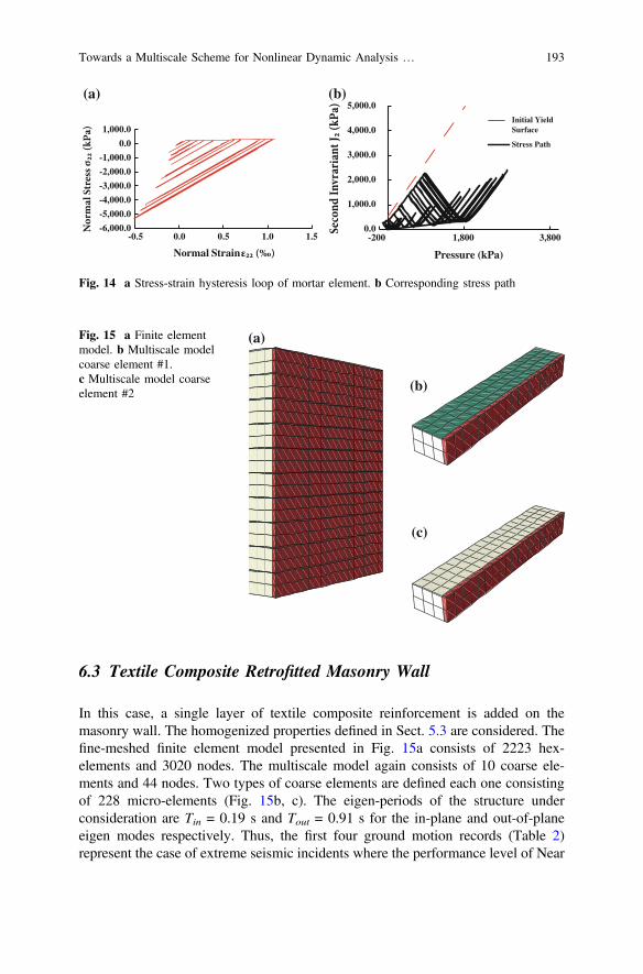
In this case, a single layer of textile composite reinforcement is added on themasonry wall. The homogenized properties defined in Sect. 5.3 are considered. Thefine-meshed finite element model presented in Fig. 15a consists of 2223 hex-elements and 3020 nodes. The multiscale model again consists of 10 coarse ele-ments and 44 nodes. Two types of coarse elements are defined each one consistingof 228 micro-elements (Fig. 15b, c). The eigen-periods of the structure underconsideration are Tin = 0.19 s and Tout = 0.91 s for the in-plane and out-of-planeeigen modes respectively. Thus, the first four ground motion records (Table 2)represent the case of extreme seismic incidents where the performance level of Near

-6,000.0

-5,000.0

-4,000.0

-3,000.0

-2,000.0

-1,000.0

0.0

1,000.0

-0.5 0.0 0.5 1.0 1.5

Normal Strain

0.0

1,000.0

2,000.0

3,000.0

4,000.0

5,000.0

-200 1,800 3,800

Pressure (kPa)

Initial YieldSurface

Stress Path

(a) (b)

Fig. 14 a Stress-strain hysteresis loop of mortar element. b Corresponding stress path

(a)

(b)

(c)

Fig. 15 a Finite elementmodel. b Multiscale modelcoarse element #1.c Multiscale model coarseelement #2


Collapse(EC8) needs to be achieved while for the rest a performance level oflimited damage should be achieved.

The derived results in terms of free end displacement time-histories are presentedin Figs. 16 and 17 for the longitudinal and out-of-plane displacement componentsrespectively. Compared to the URMW case, the peak displacements are clearlyreduced due to the increased stiffness provided from the textile composite layer.The maxima of the displacement time-histories for the two cases (URMW andRMW) are presented in Table 3. In most cases, the reduction in the absolute value ifthe out-of-plane maximum displacement of the order of 50 %. This reduction iseven larger in the Northridge and Imperial Valley(E07) case where the increasedstiffness shifts the eigen-period of the wall away from the high spectral accelerationregion of the corresponding response spectra.

Although the reduction in displacement terms is significant, damage accumu-lation is not avoided. However both the absolute value and the rate of damageaccumulation, as depicted in the corresponding hysteretic energy plot of the bottommortar layer is significantly reduced. Thus, although the textile composite layersucceeds in increasing the overall strength and stiffness of the masonry wall, only

0 5 10 15 20 25−0.03

−0.02

−0.01

0

0.01

0.02

0.03

Time [sec]

Dis

plac

emen

t [m

m]

Friuli, 1976

0 50 100 150 200−0.1

−0.05

0

0.05

0.1

Time [sec]

Dis

plac

emen

t [m

m]

ChiChi, 1999

0 5 10 15 20 25−0.06

−0.04

−0.02

0

0.02

0.04

Time [sec]

Dis

plac

emen

t [m

m]


0 5 10 15 20 25−0.05

0

0.05

Time [sec]

Dis

plac

emen

t [m

m]

Northridge, 1995

0 5 10 15 20 25−0.1

−0.05

0

0.05

0.1

Time [sec]

Dis

plac

emen

t [m

m]


0 5 10 15 20 25−0.04

−0.02

0

0.02

0.04

0.06

Time [sec]

Dis

plac

emen

t [m

m]


0 5 10 15 20 25−0.04

−0.02

0

0.02

0.04

0.06

Time [sec]

Dis

plac

emen

t [m

m]

Coyote Lake, 1979

(a)

(b) (c) (d)

(e) (f) (g)

Fig. 16 RMW—free end longitudinal displacement time histories


by slightly altering its initial thickness, it needs to be combined with conventionalmeasures to provide acceptable retrofit solutions at the Damage Limitation per-formance level (Fig. 18).

0 5 10 15 20 25−1.5

−1

−0.5

0

0.5

1

1.5

Time [sec]

Dis

plac

emen

t [m

m]

Friuli, 1976

0 50 100 150 200−2

−1

0

1

2

3

Time [sec]

Dis

plac

emen

t [m

m]

ChiChi, 1999

0 5 10 15 20 25−3

−2

−1

0

1

2

Time [sec]

Dis

plac

emen

t [m

m]


0 5 10 15 20 25−2

−1

0

1

2

Time [sec]

Dis

plac

emen

t [m

m]

Northridge, 1995

0 5 10 15 20 25−6

−4

−2

0

2

4

6

Time [sec]

Dis

plac

emen

t [m

m]


0 5 10 15 20 25−1.5

−1

−0.5

0

0.5

1

1.5

Time [sec]

Dis

plac

emen

t [m

m]


0 5 10 15 20 25−2

−1

0

1

2

Time [sec]

Dis

plac

emen

t [m

m]

Coyote Lake, 1979

(a)

(b) (c) (d)

(e) (f) (g)

Fig. 17 RMW—free end out of plane displacement time histories

Table 3 Maxima of displacement components

Ground motion record Displacement

Longitudinal (mm) Out-of-plane (mm)

URMW RMW URMW RMW

Friuli, 1976 0.04 0.03 4.43 2.19

Victoria-Mexico, 1980 0.05 0.04 4.43 2.19

Northridge, 1995 0.07 0.05 4.40 1.70

Imperial Valley(E06), 1979 0.09 0.08 8.88 5.32

Chi-Chi, 1999 0.09 0.07 3.45 2.25

Imperial Valley(E07), 1979 0.07 0.04 5.49 1.35

Coyote Lake, 1979 0.11 0.05 3.71 1.70


7 Conclusions

The nonlinear dynamic analysis of heterogeneous structures can be an arduous andtime-consuming procedure. However, it provides significant insight on thedynamics of the structural response and provides a reliable on the inelastic pro-cesses undergoing at the material level. In this work a multiscale analysis proce-dure, namely the hysteretic multiscale finite element scheme, is considered for thecomputational up-scaling of refined finite element problems. Using this method, theresponse of a natural stone masonry wall is examined under seismic excitation.Next, a layer of textile composite reinforcement is added onto the assembly and theresponse of the strengthened structure is examined. From the computational per-spective, the multiscale method used enables the engineer to run a series of analysismodels in an affordable amount of time. In terms of modeling efficiency, themultiscale model together with the hysteretic model adopted manage to capture thedynamics of the structure under consideration. The textile composite reinforcementlayer increases the stiffness of the masonry wall, while at the same time theaccumulated damage, quantified through an energy measure decreases. Futureresearch will focus on the incorporation of brittle cracking mechanisms within thepresented multi-scale formulation to further enhance the versatility of the methodand provide more accurate estimates for the dynamic response of brittle structures.

Acknowledgments This work has been carried out under the support of the Swiss NationalScience Foundation for Research Grant #200021_146996: “Hysteretic Multi/Scale Modeling forthe Reinforcing of Masonry Structures”.

0 5 10 15 20 250

50

100

150

200

250

Time [sec]

Hys

tere

tic

Ene

rgy

[kJ]

Coyote Lake, 1979

Victoria-Mexico, 1980Imp. Valley(E06), 1979

Friuli, 1979

Imp. Valley(E07), 1979

Fig. 18 Hysteretic energyaccumulation at the bottommortar layer-retrofitted wall


References

1. Chesi C, Binda L, Parisi MA (2010) Seismic damage to churches: Observations from theL’Aquila, Italy, earthquake and considerations on a case-study. Advanced Materials Research,133–134:641–646

2. Dizhur D, Ingham J, Moon L, Griffith M, Schultz A, Senaldi I, Magenes G, Dickie J, Lissel S,Centeno J, Ventura C, Leite J, Lourenco P (2011) Performance of masonry buildings andchurches in the 22 February 2011 Christchurch earthquake. Bull NZ Soc Earthq Eng 44(4):279–296

3. Binda L, Gatti G, Mangano G, Poggi C, Sacchi LG (1992) The collapse of the civic tower ofPavia: a survey of the materials and structure. Mason Int 6:11–20

4. Verstrynge E, Schueremans L, Van Gemert D, Wevers M (2009) Monitoring and predictingmasonry’s creep failure with the acoustic emission technique. NDT E Int 42(6):518–523

5. ElGawady M, Lestuzzi P, Badoux M (2005) In-plane seismic response of URM wallsupgraded with FRP. J Compos Constr 9(6):524–535

6. Habel K, Denarié E, Brühwiler E (2006) Structural response of elements combining ultrahigh-performance fiber-reinforced concretes and reinforced concrete. J Struct Eng 132(11):1793–1800

7. POLYMAST (2011) polyfunctional technical textiles for the protection and monitoring ofmasonry structures against earthquakes, final report, seventh framework programme capacitiesspecific programme research infrastructures, project no.: 227887. http://www.series.upatras.gr/polymast

8. Antonopoulos C, Triantafillou T (2003) Experimental investigation of FRP-strengthened RCbeam-column joints. J Compos Constr 7(1):39–49

9. Sivaraja SS, Thandavamoorthy TS, Vijayakumar S, Aranganathan SM, Dasarathy AK (2013)Preservation of historical monumental structures using fibre reinforced polymer (frp)—casestudies. Procedia Eng 54(0):472–479. The 2nd international conference on rehabilitation andmaintenance in civil engineering (ICRMCE)

10. Triantafillou TC, Fardis MN (1997) Strengthening of historic masonry structures withcomposite materials. Mater Struct 30(8):486–496

11. Messervey TB, Zangani D, Fuggini C (2013) Sensor embedded textiles for the reinforcement,dynamic characterisation, and structural health monitoring of masonry structures. In:Proceedings of the 5th EWSHM 2010, Sorrento, Italy, June 28–July 2, pp 1075–1082

12. Fuggini C, Chatzi E, Zangani D (2013) Combining genetic algorithms with a meso-scaleapproach for system identification of a smart polymeric textile. Comput Aided Civil InfrastructEng 28(3):227–245

13. Krebber K, Liehr S, Witt J (2012) Smart technical textiles based on fibre optic sensors. In:Proceedings of SPIE 8421, OFS2012 22nd international conference on optical fiber sensors

14. Thomas K (1996) Masonry walls: specification and design. Butterworth Heinemann, Oxford15. Morton J, Haig G (2011) Designers’ guide to Eurocode 6: design of masonry structures: EN

1996-1-1: general rules for reinforced and unreinforced masonry. ICE Publishing, London16. Binda L, Pina-Henriques J, Anzani A, Fontana A, Lourenco PB (2006) A contribution for the

understanding of load-transfer mechanisms in multi-leaf masonry walls: testing and modeling.Eng Struct 28:1132–1148

17. BS EN 1998-3 (2005) Eurocode 8: design of structures for earthquake resistance. Assessmentand retrofitting of buildings

18. American Society of Civil Engineers (2007) Seismic rehabilitation of existing buildings (41-06).American Society of Civil Engineers

19. Fardis M (2010) Advances in performance-based earthquake engineering. Springer, Berlin20. Massart TJ, Peerlings RHJ, Geers MGD (2004) Mesoscopic modeling of failure and damage-

induced anisotropy in brick masonry. Eur J Mech A Solids 72(8):1022–105921. Mojsilovic’ N (2011) Strength of masonry subjected to in-plane loading: a contribution. Int J

Solids Struct 48(6):865–873


http://www.series.upatras.gr/polymast

http://www.series.upatras.gr/polymast

22. Lourenc’o P (1996) Computational strategies for masonry structures. In: PhD thesis, DelftUniversity of Technology, The Netherlands

23. Anthoine A (1992) In-plane behaviour of masonry: a literature review. Report EUR 13840EN, commission of the European communities. Technical report, JRC—Institute for SafetyTechnology, Ispra, Italy

24. Chen S-Y, Moon FL, Yi T (2008) A macroelement for the nonlinear analysis of in-planeunreinforced masonry piers. Eng Struct 30(8):2242–2252

25. Peerlings RHJ, Geers MGD, Massart TJ (2007) An enhanced multiscale approach for masonrywall computations with localization of damage. Int J Numer Methods Eng 69(5):1022–1059

26. Massart TJ, Peerlings RHJ, Geers MGD, Gottcheiner S (2005) Mesoscopic modeling of failurein brick masonry accounting for three-dimensional effects. Eng Fract Mech 72(8):1238–1253

27. Efendiev Y, Hou TY (2009) Multiscale finite element methods. Surveys and tutorials in theapplied mathematical sciences, vol 4. Springer, New York

28. Zhang HW, Wu JK, Lv J (2012) A new multiscale computational method for elasto-plasticanalysis of heterogeneous materials. Comput Mech 49(2):149–169

29. Triantafyllou SP, Chatzi EN (2014) A hysteretic multiscale formulation for nonlinear dynamicanalysis of composite materials. Comput Mech 54(3):763–787

30. Triantafyllou S, Koumousis V (2014) Hysteretic finite elements for the nonlinear static anddynamic analysis of structures. J Eng Mech 140(6):04014025

31. Lubliner J (2008) Plasticity theory. Dover Publications, New York32. Nemat-Naser S (1982) On finite deformation elasto-plasticity. Int J Solids Struct 18

(10):857–87233. Erlicher S, Bursi O (2008) Bouc-wen type models with stiffness degradation: thermodynamic

analysis and applications. J Eng Mech 134(10):843–85534. Foliente GC, Singh MP, Noori MN (1996) Equivalent linearization of generally pinching

hysteretic and degrading systems. Earthq Eng Struct Dyn 25:611–62935. Zienkiewicz OC, Taylor RL, Zhu JZ (2005) The finite element method: its basis and

fundamentals, 6th edn. Elsevier, Amsterdam36. Armstrong PJ, Frederick CO (1966) A mathematical representation of the multiaxial

Bauschinger effect. Technical report, report RD/B/N 731 central electricity generating board37. Belytschko T, Lu YY, Gu L (1994) Element-free Galerkin methods. Int J Numer Methods Eng

37(2):229–25638. Triantafyllou SP, Koumousis VK (2012) A hysteretic quadrilateral plane stress element. Arch

Appl Mech 82(10–11):1675–168739. Washizu K (1983) Variational methods in elasticity and plasticity. Pergamon Press, Oxford40. Chopra A (2006) Dynamics of structures. Prentice Hall, New York41. Wu C, Hao H (2006) Derivation of 3d masonry properties using numerical homogenization

technique. Int J Numer Methods Eng 66(11):1717–173742. Tsai SW, Wu EM (1971) A general a general theory of strength for anisotropic materials.

J Compos Mater 5:58–8043. Flores S, Evans AG, Zok FW, Genet M, Cox B, Marshall D, Sudre O, Yang Q (2010) Treating

matrix nonlinearity in the binary model formulation for 3d ceramic composite structures.Compos A: Appl Sci Manuf 41(2):222–229

44. Jiang J-F, Wu Y-F (2012) Identification of material parameters for drucker-prager plasticitymodel for FRP confined circular concrete columns. Int J Solids Struct 49(3â€“4):445–456

45. Papanicolaou CG, Triantafillou TC, Karlos K, Papathanasiou M (2007) Textile-reinforcedmortar (TRM) versus FRP as strengthening material of URM walls: in-plane cyclic loading.Mater Struct 40(10):1081–1097

46. Hilber HM, Hughes TJR, Taylor RL (1977) Improved numerical dissipation for timeintegration algorithms in structural dynamics. Earthq Eng Struct Dyn 5(3):283–292

47. http://peer.berkeley.edu/peer_ground_motion_database/. Accessed 20 May 201448. BS EN 1998-1 (2004) Eurocode 8: design of structures for earthquake resistance—Part 1:

general rules seismic actions and rules for buildings49. Abaqus version 6.11 [Computer software]. Dassault Systmes Simulia, Providence, RI


http://peer.berkeley.edu/peer_ground_motion_database/

Date post:	20-Jul-2018
Category:	Documents
Upload:	vuque
View:	217 times
Download:	0 times

Towards a Multiscale Scheme for Nonlinear Dynamic Analysis ... · Towards a Multiscale Scheme for...

Documents