Towards artifact-free auditory evoked potentials in ...oops.uni-oldenburg.de/1195/1/viotow11.pdf ·...

Towards artifact-free auditory evoked

potentials in cochlear implant users

Der Fakultät für Mathematik und Naturwissenschaften

der Carl von Ossietkzy Universität Oldenburg

angenommene Dissertation zur Erlangung

des Grades und Titels eines

Doctor rerum naturalium (Dr. rer. nat.)

von Frau Filipa Alexandra Campos Viola

geboren am 01.01.1982 in Beja, Portugal.

Gutachter: Prof. Dr. Stefan Debener

Zweitgutachter: Prof. Dr. Christoph Herrmann

Tag der Disputation: 30.11.2011

Erklärung nach § 10 Abs. 2 der Promotionsordnung der Fakultät für Mathematik

und Naturwissenschaften der Carl von Ossietzky Universität Oldenburg vom

11. Dezember 2003

Hiermit erkäre ich, dass ich die Arbeit selbständig verfasst und nur die angegeben

Hilfsmittle benuzt habe. Die Dissertation ist bereits in Gänze veröffentlicht.

Oldenburg, den ___________ ______________________________________

Unterschrift

Erklärung nach § 10 Abs. 3 der Promotionsordnung der Fakultät für Mathematik

und Naturwissenschaften der Carl von Ossietzky Universität Oldenburg vom

11. Dezember 2003

Hiermit erkäre ich, dass die Dissertation weder in ihrer Gesamtheit noch in Teilen einer

anderen wissenschaftlichen Hochschule zur Begutachtung in einem Promotionsverfahren

vorliegt oder vorgelegen hat.

Oldenburg, den ___________ ______________________________________

Unterschrift

Abstract

Cochlear implants (CI) are neural prostheses that mimic the function of the healthy

cochlea and deliver electrical stimulation to the auditory nerve, allowing individuals

suffering from sensorineural hearing loss to recover a large amount of hearing function.

Although CIs are regarded as one of the great achievements of modern medicine, the

outcomes after implantation are variable, and it is not well understood how the auditory

cortex adapts to the electrical stimulation delivered by the CI. An objective and non-

invasive method for assessing auditory rehabilitation after implantation is by using

electroencephalography (EEG) to measure auditory evoked potentials (AEPs). However

EEG signals consist of a mixture of an unknown number of brain and non-brain

contributions, the latter also called artifacts. The non-brain signals can be divided into

two categories: biological and non-biological artifacts. CI devices cause non-biological

electrical artifacts

These artifacts corrupt and mask the AEPs, since they are time-locked to auditory stimuli,

and therefore cannot be attenuated using standard techniques such as filtering or

averaging. A particularly promising technique to deal with CI artifacts is independent

component analysis (ICA). This technique can disentangle multi-channel EEG signals

into a number of artifacts and brain-related signals, also called independent components

(ICs). When using an ICA-based attenuation approach, the ICs related to artifacts can be

removed, and a corrected version of the original EEG signal can be obtained. However,

the identification and interpretation of ICs is time-consuming and involves subjective

decision making.

In Study 1 a tool tailored to identify ICs representing eye blinks, lateral movements and

heartbeat artifacts was developed and validated. The tool is based on the correlation of

ICA inverse weights, also called IC scalp maps, with a user-defined template map, thus it

was named CORRMAP. The performance of the tool was compared with the

performance of 11 raters from different laboratories familiar with ICA. The overlap

between ICs selected by CORRMAP and by the raters was substantial, providing

evidence that the tool offers an efficient way of attenuating these particular artifacts.

In Study 2 the effects of CI artifact attenuation on AEP quality were investigated in a

sample of 18 adult post-lingually deafened individuals, using different types of CIs. Here

ICs related to CI artifacts were selected by visual inspection and AEPs were

reconstructed. It was found that AEPs from CI users were systematically correlated with

age, indicating that individual differences were well preserved. CI users with large signal-

to-noise ratio AEPs were characterized by a significantly shorter duration of deafness.

The ability of ICA in attenuating the CI artifact while preserving the AEPs was evaluated

using a simulation study where datasets from normal hearing listeners were previously

contaminated with CI artifacts. Results revealed very high spatial correlations between

original and recovered normal hearing AEPs.

In Study 3 a tool tailored to identify ICs related to the CI artifact was developed and

validated. The CI Artifact Correction (CIAC) algorithm evaluates temporal and

topographical properties of ICs, in order to objectively identify components representing

the CI artifact. CIAC was tested on EEG data from two different experiments. The first

consisted of datasets from the 18 CI users evaluated in Study 2. The second consisted of

independent datasets recorded from 12 out of the 18 CI users at a different time point

after implantation. CIAC sensitivity and specificity was compared to the manual IC

selection performed by two experts. Results revealed both good sensitivity and

specificity. A correlation between age and AEP amplitude was observed, replicating the

findings from Study 2 and confirming the algorithm’s validity. High test-retest reliability

for AEP N1 amplitudes and latencies also suggested that CIAC based attenuation reliably

preserves plausible individual response characteristics.

Overall the results confirm that after ICA-based attenuation of CI artifacts, good quality

AEPs can be recovered. This is highly important as it facilitates the objective, non-

invasive study of auditory cortex function in CI users. With CORRMAP and CIAC

efficient, convenient and objective tools were developed to attenuate biological and CI

artifacts in EEG data. Both tools have been published and can be used by interested

scientists.

Zusammenfassung

Cochlea Implantate (CI) sind Innenohrprothesen mit denen die Funktion einer gesunden

Cochlea nachgeahmt wird. Dies geschieht durch eine elektrische Stimulation des

auditorischen Nerven. Mit Hilfe von CIs kann bei Personen mit einem sensorineuralen

Hörverlust der Höreindruck zu einem großen Teil wieder hergestellt werden. Obwohl CIs

als eine der wichtigen Errungenschaften der modernen Medizin gelten, ist der Erfolg der

Implantation sehr variabel. Auch ist bisher wenig darüber bekannt, inwieweit sich der

auditorische Kortex an das elektrische Signal des CIs anpasst. Die

Elektroenzephalographie (EEG) ist eine objektive und nicht invasive Methode mit der

mittels akustisch evozierter Potenziale (AEPs) die auditorische Rehabilitation nach der

Implantation eingeschätzt werden kann. Zu dem an der Kopfoberfläche gemessenen EEG

Signal tragen jedoch verschiedene zerebrale und nicht zerebrale Aktivitäten bei, letztere

werden auch als Artefakte bezeichnet. Diese können wiederum unterteilt werden in

biologische und nicht biologische Artefakte. CIs verursachen nicht biologische,

elektrische Artefakte.

CI-Artefakte verschlechtern und überdecken die AEPs. Da sie zeitlich an den akustischen

Stimulus gekoppelt sind können sie jedoch nicht mittels der gängigen Techniken der

Artefaktbereinigung wie z.B. Filtern oder Mittelung reduziert werden. Ein sehr

vielversprechender alternativer Ansatz zur Korrektur der durch CIs verursachten

elektrischen Artefakte ist die independent component analysis (ICA, unabhängige

Komponenten Analyse). Mit Hilfe der ICA können verschiedene Artefakte und

gehirnbezogene Signale aus einem Multikanal-EEG-Signal extrahiert werden, die

sogenannten independent components (ICs, unabhängige Komponenten). Werden die

artefaktbezogenen ICs aus dem EEG entfernt erhält man eine korrigierte, weitgehend

artefaktfreie Version des EEGs. Ein großes Problem stellt jedoch die Identifikation und

Interpretation der ICs dar, da sie einerseits sehr zeitaufwendig ist und andererseits häufig

subjektive Entscheidungen beinhaltet.

In Studie 1 wurde CORRMAP entwickelt und validiert. CORRMAP ist ein Verfahren mit

dessen Hilfe die Identifikation von ICs für die häufigsten biologischen Artefakte

Blinzeln, seitliche Augenbewegungen und Herzschlag möglich ist. Grundlage von

CORRMAP ist die Korrelation der inversen Gewichte aller ICs einer ICA mit den

inversen Gewichten einer durch den Nutzer ausgewählten, für den jeweiligen Artefakt

prototypischen IC. Das inverse Gewicht einer IC reflektiert die topographische Verteilung

der IC und wird deswegen auch als IC scalp map bezeichnet. Für Die Validierung von

CORRMAP wurden drei verschiedene Datensätze herangezogen. Die von CORRMAP

identifizierten Artefakt-ICs wurden mit den von 11 unabhängigen Experten identifizierten

Artefakt-ICs verglichen. Die Übereinstimmung zwischen CORRMAP und den Experten

war beachtlich. Dies zeigt das häufige biologische EEG Artefakte mit CORRMAP

effizient identifiziert und reduziert werden können.

In Studie 2 wurden an einer Stichprobe von 18 postlingual ertaubten Erwachsenen die

Effekte der CI-Artefaktreduktion auf die Qualität der AEPs untersucht. Dabei wurden die

zu den CI-Artefakten gehörenden ICs manuell selektiert und entfernt, und die AEPs

rekonstruiert. Das Signal-Rausch-Verhältnis der korrigierten AEPs war deutlich besser

bei CI-Trägern mit kürzerer Dauer der Gehörlosigkeit. Die Amplitude der rekonstruierten

AEPs der CI-Nutzer zeigte die typische systematische Korrelation mit dem Alter. Die

Bewahrung individueller Unterschiede im AEP deutet auf eine gute Qualität der

rekonstruierten AEPs hin. Mit Hilfe einer Simulation wurde weiterhin evaluiert inwieweit

die ICA CI-Artefakte verringert und gleichzeitig die AEPs erhält. Datensätze von normal

hörenden Personen wurden mit einem CI-Artefakt belegt. Der CI-Artefakt wurde mittels

ICA aus den simulierten CI-Datensätzen entfernt. Rekonstruiert und originale AEPs

wurden miteinander korreliert. Dabei wurden sehr hohe räumliche Korrelationen

zwischen den ursprünglichen und den wiederhergestellten AEPs erzielt. Dies ist ein

weiterer Beleg für die gute Qualität der rekonstruierten AEPs.

In Studie 3 wurde ein CI-Artefakt-Korrektur-Algorithmus (CIAC, CI Artifact Correction)

entwickelt und validiert. CIAC bewertet zeitliche und topographische Eigenschaften der

ICs, um CI-bezogene Komponenten auf objektive Weise zu identifizieren. CIAC wurde

an EEG-Daten aus zwei verschiedenen, unabhängigen Experimenten getestet. Bei dem

ersten Datensatz handelt es sich um die für Studie 2 erhobenen Daten. Der zweite

Datensatz enthält Daten für 12 der 18 CI-Nutzer aus Studie 2. Diese wurden in einem

unabhängigen Experiment erhoben. Die Sensitivität und Spezifität von CIAC wurde

verglichen mit einer manuellen IC-Selektion durch zwei Experten. Die Ergebnisse zeigen

sowohl eine gute Sensitivität als auch eine gute Spezifität von CIAC. Auch in dieser

Studie zeigte sich eine Korrelation zwischen dem Alter und der Amplitude der AEPs,

wodurch das Ergebnis aus Studie 2 repliziert und die Validität des Algorithmus bestätigt

wurde. Die hohe Test-Retest-Reliabilität zwischen den beiden Datensätzen für die N1-

Amplitude und Latenz der AEPs weist darauf hin, dass bei einer Reduktion des CI-

Artefaktes basierend auf CIAC die individuellen Merkmale der Reaktionen erhalten

bleiben.

Die Ergebnisse der vorliegenden Arbeit belegen, dass durch eine ICA-basierte Reduktion

von CI-Artefakten AEPs in einer guten Qualität wiederhergestellt werden können. Dies

ist die Voraussetzung für eine objektive, nicht invasive Untersuchung der Funktionen des

auditorischen Kortex bei CI-Nutzern. Mit CORRMAP und CIAC wurden effiziente,

praktische und objektive Verfahren zur Identifikation und somit Reduktion von

biologischen und CI-Artefakten entwickelt. Beide Verfahren wurden veröffentlicht und

sind somit für interessierte Wissenschaftler zugänglich.

vii

Contents

Acknowledgements ............................................................................................... xi

List of figures ....................................................................................................... xiii

List of tables ......................................................................................................... xv

List of abbreviations .......................................................................................... xvii

1. Overview ............................................................................................................. 1

Chapter-by-chapter overview ................................................................................... 1 1.1.

2. Introduction ........................................................................................................ 3

1BElectroencephalography .......................................................................................... 3 2.1.

2.1.1. 4BRecording the electroencephalogram ............................................................... 3

2.1.2. 5BEvent related potentials .................................................................................... 6

2.1.3. 6BArtifacts in EEG recordings ........................................................................... 11

2BIndependent component analysis........................................................................... 12 2.2.

2.2.1. 7BApplication to EEG data................................................................................. 14

2.2.2. 8BEEG artifact attenuation ................................................................................. 17

2.2.3. 9BPractical problems .......................................................................................... 20

3BAssessment of auditory evoked potentials in cochlear implant users ................... 21 2.3.

2.3.1. 10BThe human auditory system ........................................................................... 22

2.3.2. 11BDeafness: etiologies and treatments ............................................................... 24

2.3.3. 12BRestoration of auditory function with cochlear implants ............................... 27

2.3.4. 13BAuditory evoked potentials as an objective assessment of auditory

rehabilitation ............................................................................................................. 32

2.3.5. 14BEEG recordings from cochlear implant users ................................................. 36

3. Objectives ......................................................................................................... 41

4. Study 1: Semi-automatic identification of independent components

representing EEG artifact ................................................................................... 43

viii

Abstract .................................................................................................................. 43 4.1.

Introduction ............................................................................................................ 44 4.2.

Methods .................................................................................................................. 47 4.3.

4.3.1. CORRMAP description .................................................................................. 47

4.3.2. Validation study .............................................................................................. 49

4.3.3. Statistical analysis ........................................................................................... 50

Results .................................................................................................................... 51 4.4.

Discussion .............................................................................................................. 58 4.5.

5. Study 2: Uncovering auditory evoked potentials from cochlear implant

users with independent component analysis ..................................................... 63

Abstract .................................................................................................................. 63 5.1.

Introduction ............................................................................................................ 64 5.2.

Methods .................................................................................................................. 66 5.3.

5.3.1. Participants ...................................................................................................... 66

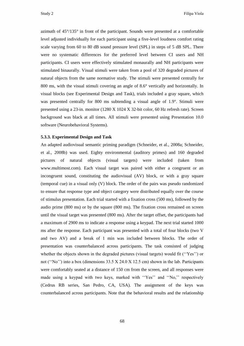
5.3.2. Stimuli ............................................................................................................. 67

5.3.3. Experimental Design and Task ....................................................................... 68

5.3.4. EEG Recording ............................................................................................... 69

5.3.5. Data Processing ............................................................................................... 69

5.3.6. ICA sensitivity ................................................................................................ 70

5.3.7. AEP quality ..................................................................................................... 70

5.3.8. ICA specificity ................................................................................................ 71

5.3.9. Statistical Analysis .......................................................................................... 72

Results .................................................................................................................... 72 5.4.

5.4.1. ICA Sensitivity ................................................................................................ 72

5.4.2. AEP quality ..................................................................................................... 73

5.4.3. ICA Specificity................................................................................................ 76

Discussion .............................................................................................................. 79 5.5.

ix

6. Study 3: Automatic attenuation of cochlear implant artifacts for the

evaluation of late auditory evoked potentials .................................................... 83

Abstract .................................................................................................................. 83 6.1.

Introduction ............................................................................................................ 85 6.2.

Methods .................................................................................................................. 87 6.3.

6.3.1. CIAC description ............................................................................................ 87

6.3.2. Environmental Sounds Study (ESS) ............................................................... 90

6.3.2.1. Subjects .................................................................................................... 90

6.3.2.2. Stimuli and Task ...................................................................................... 91

6.3.2.3. Electrophysiology recordings ................................................................... 91

6.3.2.4. Data processing ........................................................................................ 91

6.3.2.5. Automatic identification of CI artifact related ICs using CIAC............... 92

6.3.2.6. Auditory evoked potential quantification ................................................. 92

6.3.3. Tones and Noise Study (TNS) ........................................................................ 92

6.3.3.1. Subjects .................................................................................................... 92

6.3.3.2. Stimuli and Task ...................................................................................... 93

6.3.3.3. Electrophysiology recordings ................................................................... 93

6.3.3.4. Data Analysis ........................................................................................... 93

6.3.3.5. Automatic identification of CI artifact related ICs using CIAC............... 93

6.3.3.6. Auditory evoked potential quantification ................................................. 93

6.3.4. Statistical Analysis .......................................................................................... 94

6.3.5. Test-retest reliability ....................................................................................... 94

Results .................................................................................................................... 94 6.4.

6.4.1. Environmental Sounds Study (ESS) ............................................................... 94

6.4.2. Tones and Noise Study (TNS) ........................................................................ 96

6.4.3. Test-retest reliability ....................................................................................... 97

Discussion .............................................................................................................. 98 6.5.

Conclusion ........................................................................................................... 100 6.6.

x

7. General Discussion ......................................................................................... 101

Summary .............................................................................................................. 101 7.1.

Towards automatic identification of artifacts in EEG using ICA ........................ 102 7.2.

Investigation of auditory rehabilitation after cochlear implantation .................... 106 7.3.

Outlook................................................................................................................. 108 7.4.

References ........................................................................................................... 113

Curriculum vitae ................................................................................................ 125

xi

Acknowledgements

This work is dedicated to my “families”, to whom I’m truly grateful.

First of all it is dedicated to my parents and my sister. Second it is dedicated to my

“Doktorvater”, Stefan Debener, and my “Doktorbruder”, Jeremy Thorne. Both have been

by my side since the very first day, and make it all possible.

It is also dedicated to four other “families”:

In Southampton: Jessica de Boer, Jemma Hine, Brigitte Lavoie, Roger Thornton, Angie

Barks, Sue Mooney, David Olley, Stefan Bleeck, Julie Eyles, and Ragvinder Pahal.

In Jena: Janneke Terhaar, Thomas Weiss, Teresa Görtz, Ralph Huonker, Stefan Clauß,

Thomas Heuchel, Christoph Kurzbuch, Ana Magina, Artur Moro, Luis Figueiredo, and

Marie Fischer.

In Oldenburg: Maarten De Vos, Pascale Sandmann, Nadine Hauthal, Jolanda Janson,

Janani Dhinakaran, Cornelia Kranczioch, Reiner Emkes, Alexander Förstel, and Ulrike

Bayer.

My new family: Michael Groen and our future family.

I must also thank the Fundacao para a Ciencia e Tecnologia, Lisbon, Portugal for the

financial support that enabled me to develop this project (SFRH/BD/37662/2007).

A special thanks to Helio Pais, who convinced me to start a “PhD”.

A special thanks to all who have inspired me.

xii

xiii

List of figures

Figure 2.1 The generation of open electrical fields by synaptic currents in PNs ................ 4

Figure 2.2 Illustration of different procedures involved in recording human ERPs ........... 6

Figure 2.3 Illustration of the ERP model ............................................................................ 7

Figure 2.4 Mathematical relationship between SNR and number of trials ......................... 7

Figure 2.5 Auditory evoked potentials recorded from a NH adult .................................... 10

Figure 2.6 ICA assumptions applied to EEG data ............................................................ 15

Figure 2.7 Schematic outline illustrating the application of ICA to EEG data ................. 16

Figure 2.8 Typical EEG artefacts as identified by ICA .................................................... 18

Figure 2.9 Illustration of artifact removal by means of ICA ............................................. 19

Figure 2.10 Three phases defining the major events in the development of CIs .............. 22

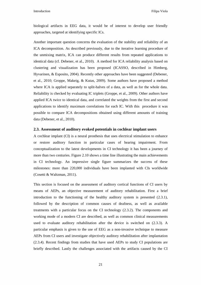
Figure 2.11 Anatomy of the peripheral auditory system ................................................... 23

Figure 2.12 Auditory pathways of the human brain .......................................................... 24

Figure 2.13 Illustration of sensorineural hearing loss ...................................................... 25

Figure 2.14 Treatment of hearing impairment .................................................................. 26

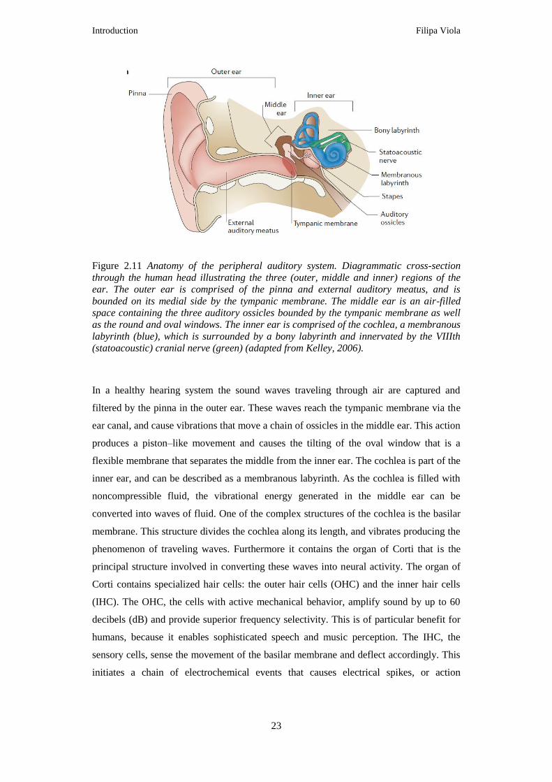
Figure 2.15 Components of modern cochlear implant systems ........................................ 28

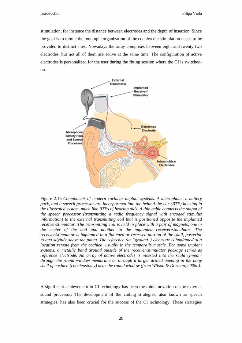
Figure 2.16 Individual subject performance for speech recognition tests ......................... 30

Figure 2.17 Example of a participant undergoing a MEG recording ................................ 36

Figure 2.18 EEG recording from a CI user ....................................................................... 38

Figure 2.19 AEPs before ICA-based artifact reduction .................................................... 39

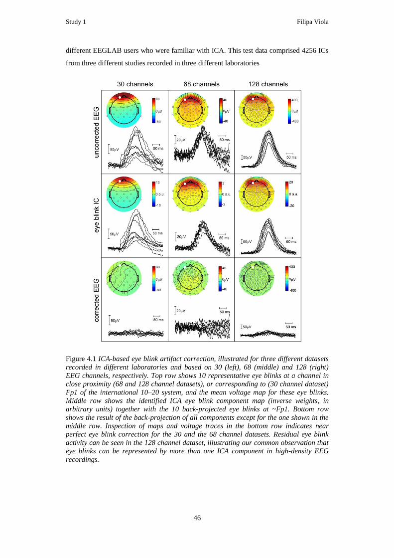
Figure 4.1 ICA-based eye blink artifact correction ........................................................... 46

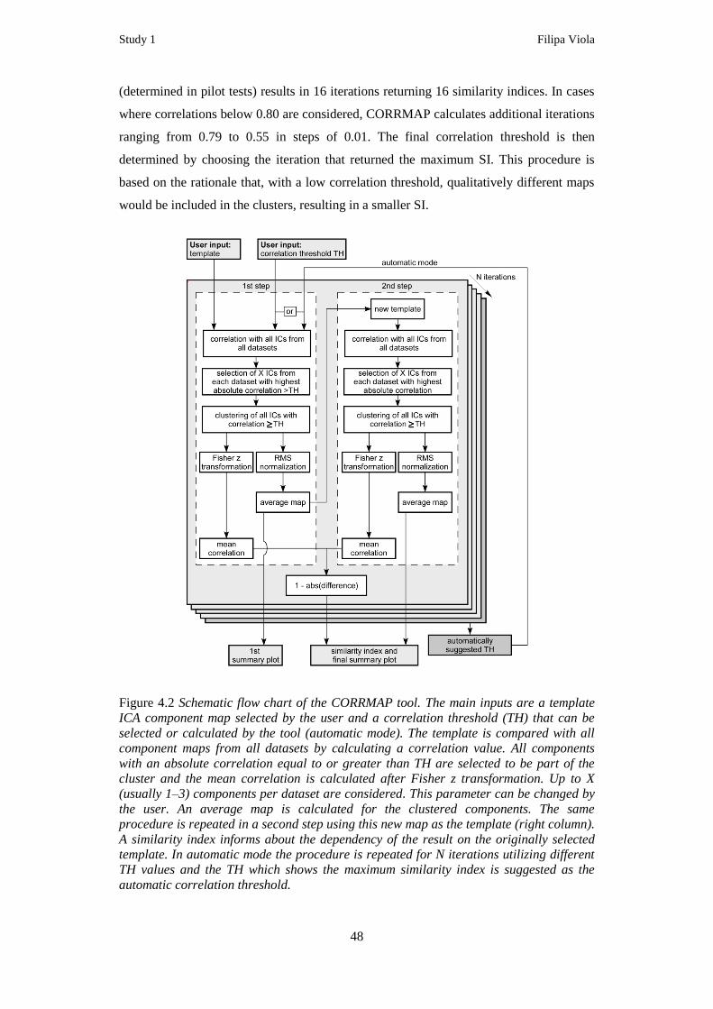
Figure 4.2 Schematic flow chart of the CORRMAP tool ................................................. 48

Figure 4.3 Example CORRMAP output figure ................................................................. 53

Figure 4.4 CORRMAP validation result for eye blink ICA components ........................ 55

Figure 4.5 Inconsistencies between CORRMAP results and user selection ..................... 56

Figure 4.6 CORRMAP validation for lateral eye movement and heartbeat artifact ......... 57

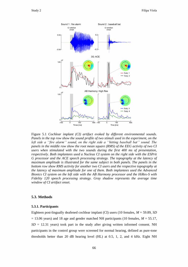
Figure 5.1 Cochlear implant artifact evoked by different environmental sounds ............. 66

Figure 5.2 Box plots showing median cochlear artifact (CI) attenuation rate .................. 73

Figure 5.3 AEPs for all 36 participants ............................................................................. 74

Figure 5.4 Correlation between N1-P2 peak-to-peak amplitude and subject age ............. 75

xiv

Figure 5.5 Comparison of clinical profiles from CI .......................................................... 76

Figure 5.6 Evaluation of ICA specificity – Simulation ..................................................... 77

Figure 5.7 Evaluation of ICA specificity – VEPs……… ................. ……………………78

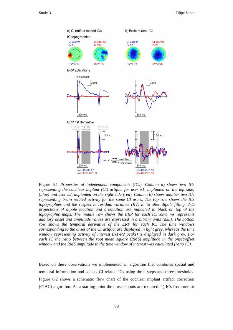
Figure 6.1 Properties of independent components…………………………… ................ 88

Figure 6.2 Schematic flow chart of CIAC algorithm……………………................... ..... 90

Figure 6.3 Summary of AEPs for ESS......................................................................... ..... 95

Figure 6.4 Comparison of AEPs reconstructed for ESS and for TNS……………… ...... 97

Figure 6.5 Test-retest reliability for the N1 peak amplitude and latency……….………98

xv

List of tables

Table 2.1 Example of AEP studies with adult CI users .................................................... 34

Table 2.2 Example of AEP studies with children using CIs ............................................. 35

Table 4.1 Number of ICs Identified by CORRMAP and by Users ................................... 52

Table 4.2 Degree of Association Between CORRMAP Clusters and Users ..................... 54

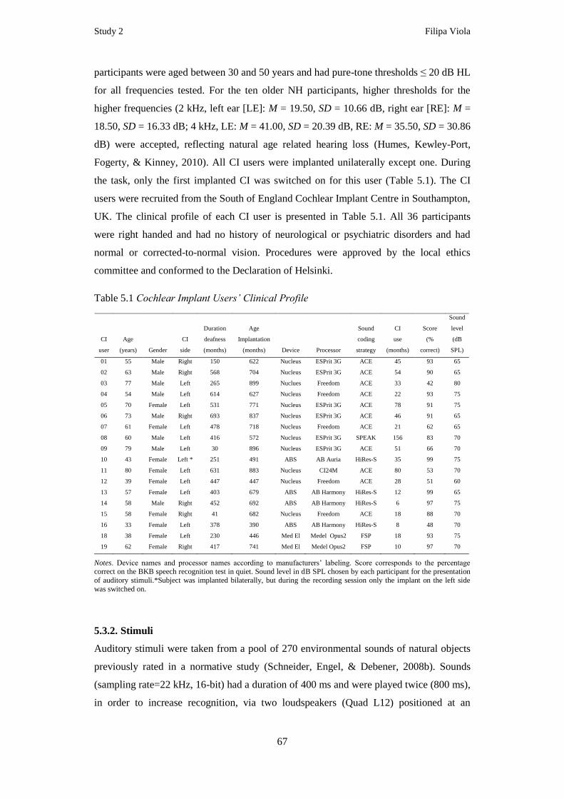
Table 5.1 Cochlear Implant Users’ Clinical Profile .......................................................... 67

Table 5.2 AEP Parameterization ....................................................................................... 73

Table 5.3 Mean RMS Across Channels for VEP Peak Latencies and Amplitudes ........... 78

Table 6.1 Mean N1-P2 peak-to-peak amplitude and N1 and P2 peak latencies ............... 96

xvi

xvii

List of abbreviations

ACE – Advanced combination encoders

AEP – Auditory evoked potential

ARHL – Age related hearing loss

AV – Audiovisual

BKB – Bamford-Kowal-Bench

BKB-SIN – Bamford-Kowal-Bench Speech-in-Noise (BKB-SIN)

BOLD – Blood-oxygenation-level-dependent

BTE – Behind-the-ear

CI – Cochlear implant

CIAC – Cochlear implant artifact correction

CNC – Consonant-nucleus-consonant

dB – Decibel

ECG – Electrocardiography

EEG – Electroencephalography

ERP – Event-related potential

ESS – Environmental sounds study

FDA – Food and drug administration

FSP – Fine structure processing

fMRI – Functional magnetic resonance imaging

HEP – Heartbeat evoked potential

HINT – Hearing in noise test

HiRes-S – High resolution with fidelity 120

HL – Hearing level

IC – Independent component

ICA – Independent component analysis

IHC – Inner hair cells

LE – Left ear

xviii

M – Mean

MCG – Magnetocardiography

MEG – Magnetoencephalography

Mdn – Median

MLR – Middle latency response

MMN – Mismatch negativity

MRI – Magnetic resonance imaging

NH – Normal hearing

NIRS – Near-infrared spectroscopy

OHC – Outer hair cells

ODR – Optimized differential reference

PC – Personal computer

PET – Positron emission tomography

PN – Pyramidal neuron

RE – Right ear

RF – Radio frequency

RMS – Root mean square

RV – Residual variance

SD – Standard deviation

SI – Similarity index

SNHL – Sensorineural hearing loss

SNR – Signal-to-noise ratio

SPL – Sound pressure level

SPEAK – Spectral peaking code

TNS – Tones and noise study

V – Visual

VEP – Visual evoked potential

UK – United Kingdom

USA – United States of America

WHO – World health organization

Overview Filipa Viola

1

1. Overview

The structure of this thesis consists of an introduction, followed by a chapter describing

the main objectives of the empirical studies, and then three independent chapters with a

detailed description of each study. The last chapter consists of a general discussion that

concludes the thesis. The work presented here was developed between 2008 and 2011 in

the following research institutes: Medical Research Council, Institute of Hearing

Research, Southampton, UK (Jan 2008 – Dec 2008); Biomagnetic Centre, Department of

Neurology, Jena University Hospital, Germany (Jan 2009 – Dec 2009); Neuropsychology

Laboratory, Department of Psychology, University of Oldenburg, Germany (Jan 2010 –

present).

Chapter-by-chapter overview 1.1.

Chapter 2

This is an introductory chapter where background information about the main techniques

and methods used in the empirical studies, e.g. electroencephalography (EEG), auditory

evoked potentials (AEPs), and independent component analysis (ICA), is briefly

described. The assessment of AEPs in cochlear implant (CI) users is discussed. A

literature overview is provided and CI technology is described.

Chapter 3

The motivation for the three empirical studies presented in the following chapters is

described. Two studies focused on the improvement of signal processing tools that need

to be applied when using multi-channel EEG and AEPs to investigate auditory cortical

rehabilitation in CI users. The other evaluated the quality of AEPs from CI users and

further validated the use of an ICA-based approach to attenuate CI artifacts from EEG

recordings.

Chapter 4

This chapter describes Study 1 where an ICA-based tool, named CORRMAP, was

developed to select objectively ICs representing ocular and heartbeat activity. The main

input of the tool is the scalp map from an IC representing one of the target artifacts. This

template is correlated with the scalp maps from other ICs. The selected ICs are those for

which the correlation value exceeds a threshold. The performance of the tool was

compared with 11 independent raters familiar with ICA. Results of the validation study

and the advantages of this new tool are discussed.

Overview Filipa Viola

2

Chapter 5

This chapter describes Study 2 where 68-channnel EEG was recorded from 18 adult post-

lingually deafened CI users stimulated with environmental sounds. First, the ability of

ICA to attenuate electrical artifacts caused by the CI was investigated. Second, the ability

to preserve the brain responses of interest in the EEG data after ICA-based attenuation

was investigated. Third, the quality of reconstructed AEPs was assessed using signal-to-

noise ratio (SNR) measurements. The relationship between AEPs and clinical parameters

was also assessed. The validity of ICA as a suitable technique to attenuate CI artifacts

while preserving brain responses is discussed. The application of AEPs as an objective

measurement of auditory rehabilitation in CI users is also highlighted.

Chapter 6

This chapter describes Study 3 where an ICA-based algorithm tailored to select ICs

representing the CI artifact was implemented. The algorithm, called Cochlear Implant

Artifact Correction (CIAC), evaluates temporal and spatial information from the ICs, in

order to find those ICs representing the CI artifact. CIAC was evaluated using two

different EEG study sets. The sensitivity and specificity of CIAC was compared to the

manual selection performed by two experts. AEPs were reconstructed after automatic CI

artifact attenuation and evaluated. The advantages of CIAC and the AEP findings are

discussed.

Chapter 7

A general discussion of the results and their implications concludes the thesis. First the

main results from the three empirical studies are summarized. The tools developed in

Study 1 and Study 3, due to their similar frameworks, are jointly discussed. The relevance

of the AEP findings from Study 2 and Study 3 is reviewed. Lastly the further validation

and implementation of ICA-based tools to select objectively ICs is also discussed, and

future directions for AEP studies with CI samples are suggested.

Introduction Filipa Viola

3

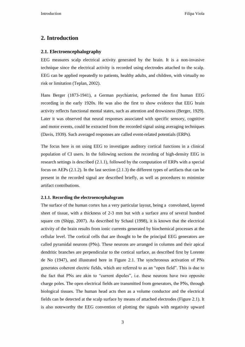
2. Introduction

1BElectroencephalography 2.1.

EEG measures scalp electrical activity generated by the brain. It is a non-invasive

technique since the electrical activity is recorded using electrodes attached to the scalp.

EEG can be applied repeatedly to patients, healthy adults, and children, with virtually no

risk or limitation (Teplan, 2002).

Hans Berger (1873-1941), a German psychiatrist, performed the first human EEG

recording in the early 1920s. He was also the first to show evidence that EEG brain

activity reflects functional mental states, such as attention and drowsiness (Berger, 1929).

Later it was observed that neural responses associated with specific sensory, cognitive

and motor events, could be extracted from the recorded signal using averaging techniques

(Davis, 1939). Such averaged responses are called event-related potentials (ERPs).

The focus here is on using EEG to investigate auditory cortical functions in a clinical

population of CI users. In the following sections the recording of high-density EEG in

research settings is described (2.1.1), followed by the computation of ERPs with a special

focus on AEPs (2.1.2). In the last section (2.1.3) the different types of artifacts that can be

present in the recorded signal are described briefly, as well as procedures to minimize

artifact contributions.

2.1.1. 4BRecording the electroencephalogram

The surface of the human cortex has a very particular layout, being a convoluted, layered

sheet of tissue, with a thickness of 2-3 mm but with a surface area of several hundred

square cm (Shipp, 2007). As described by Schaul (1998), it is known that the electrical

activity of the brain results from ionic currents generated by biochemical processes at the

cellular level. The cortical cells that are thought to be the principal EEG generators are

called pyramidal neurons (PNs). These neurons are arranged in columns and their apical

dendritic branches are perpendicular to the cortical surface, as described first by Lorente

de No (1947), and illustrated here in Figure 2.1. The synchronous activation of PNs

generates coherent electric fields, which are referred to as an “open field”. This is due to

the fact that PNs are akin to “current dipoles”, i.e. these neurons have two opposite

charge poles. The open electrical fields are transmitted from generators, the PNs, through

biological tissues. The human head acts then as a volume conductor and the electrical

fields can be detected at the scalp surface by means of attached electrodes (Figure 2.1). It

is also noteworthy the EEG convention of plotting the signals with negativity upward


4

used in Figure 2.1. This convention dates to the 1930s when ERP research started. It

seems that in those days neurophysiologists plotted negative upward, possibly because

this allowed an action potential to be plotted as an upward-going spike (Luck, 2005, cf.

chapter 1). The negative upward convention will be used through this text.

Figure 2.1 The generation of open electrical fields by synaptic currents in pyramidal

neurons. The EEG electrode (referenced to a second electrode some distance away)

measures this pattern through thick tissue layers. Notice the EEG convention of plotting

the signals with negativity upward (blue) (adapted from Bear, Connors, & Paradiso,

2007). 1

The size, shape and duration of the EEG waves are influenced by the orientation of the

neural generators, their synchrony, and their distance to the recording electrode (Schaul,

1998). However the estimation of the neuronal sources responsible for a given scalp

potential is not trivial, since there is no unique solution. The number of possible source

configurations that give rise to a given set of measured scalp potentials is infinite and

assumptions about the nature of the sources are required (Slotnick, 2005). These

assumptions imply for instance a priori knowledge of functional neural anatomy, and

conductance properties of biological tissues. This framework is called the inverse

1 All figures reproduced or adapted in this work were reprinted with the permission from publishers or

authors.


5

problem of EEG. Details can be found in specialized text books (Handy, 2005; Lopes da

Silva, 2010; Luck, 2005).

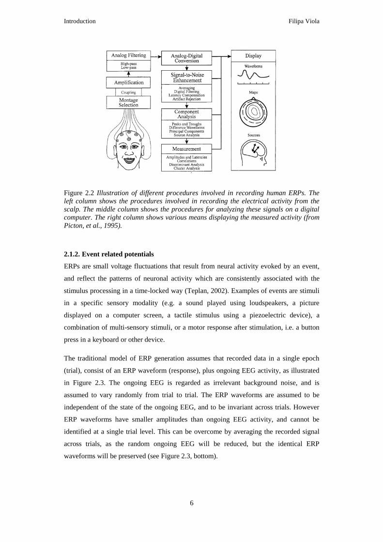
A schematic of the different steps involved both in the EEG recording session and in the

analysis of the data is shown in Figure 2.2. The first step consists of attaching electrodes

to the scalp using a conductive gel or paste which establishes the connection between the

electrode and the skin, while the final goal is to evaluate brain activity. The steps

inbetween involve the use of electronic devices such as amplifiers with filters, analog-

digital converters, recording devices, and at the last stage a computer to store the data and

to perform the signal processing analysis. Briefly, the electrodes read the signal from the

scalp surface, amplifiers enhance the microvolt signals into a range where they can be

digitalized accurately, the converter changes signals from analog to digital form, and a

computer using suitable recording software stores and displays obtained data (Teplan,

2002).

The minimum number of electrodes necessary to perform an EEG recording is three:

ground, reference and active electrode. A basic electrical circuit needs to be created in

order to measure potential changes over time between the pair active-ground and the pair

reference-ground. There is no agreement for the placement of the reference electrode,

common locations being the ear lobe or the nose tip, as neuronal activity is assumed to be

low at these locations. The quality of the recorded signal is highly dependent on the

proper function and preparation of the recording electrodes. For instance, it is important

that the impedance at electrode sites is low. However recommendations vary according to

the type of EEG system. Other authors have also investigated in detail the effects of

electrode impedance on data quality (Kappenman & Luck, 2010).

Many EEG systems allow simultaneous recording from between 30 and 256 electrodes,

which can be arranged in different montages. The era of high-density EEG recordings

was made possible due to the rapid advances in computer technology observed in the last

two decades. These high-density recordings have the advantage of allowing the

computation of 2D or 3D topographic maps, which complement the high temporal

resolution, and can contribute to a better estimation of the localization of neural

generators. On the other hand, the larger the number of electrodes, the longer the

preparation of the recording session becomes, as well as the computation time needed for

the analysis. More details about recording procedures and electrode montages have been

discussed in the literature (Handy, 2005; Luck, 2005; Picton, Lins, & Scherg, 1995).


6

Figure 2.2 Illustration of different procedures involved in recording human ERPs. The

left column shows the procedures involved in recording the electrical activity from the

scalp. The middle column shows the procedures for analyzing these signals on a digital

computer. The right column shows various means displaying the measured activity (from

Picton, et al., 1995).

0F

2.1.2. 5BEvent related potentials

ERPs are small voltage fluctuations that result from neural activity evoked by an event,

and reflect the patterns of neuronal activity which are consistently associated with the

stimulus processing in a time-locked way (Teplan, 2002). Examples of events are stimuli

in a specific sensory modality (e.g. a sound played using loudspeakers, a picture

displayed on a computer screen, a tactile stimulus using a piezoelectric device), a

combination of multi-sensory stimuli, or a motor response after stimulation, i.e. a button

press in a keyboard or other device.

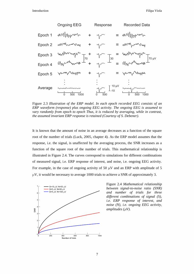
The traditional model of ERP generation assumes that recorded data in a single epoch

(trial), consist of an ERP waveform (response), plus ongoing EEG activity, as illustrated

in Figure 2.3. The ongoing EEG is regarded as irrelevant background noise, and is

assumed to vary randomly from trial to trial. The ERP waveforms are assumed to be

independent of the state of the ongoing EEG, and to be invariant across trials. However

ERP waveforms have smaller amplitudes than ongoing EEG activity, and cannot be

identified at a single trial level. This can be overcome by averaging the recorded signal

across trials, as the random ongoing EEG will be reduced, but the identical ERP

waveforms will be preserved (see Figure 2.3, bottom).


7

Figure 2.3 Illustration of the ERP model. In each epoch recorded EEG consists of an

ERP waveform (response) plus ongoing EEG activity. The ongoing EEG is assumed to

vary randomly from epoch to epoch Thus, it is reduced by averaging, while in contrast,

the assumed invariant ERP response is retained (Courtesy of S. Debener).

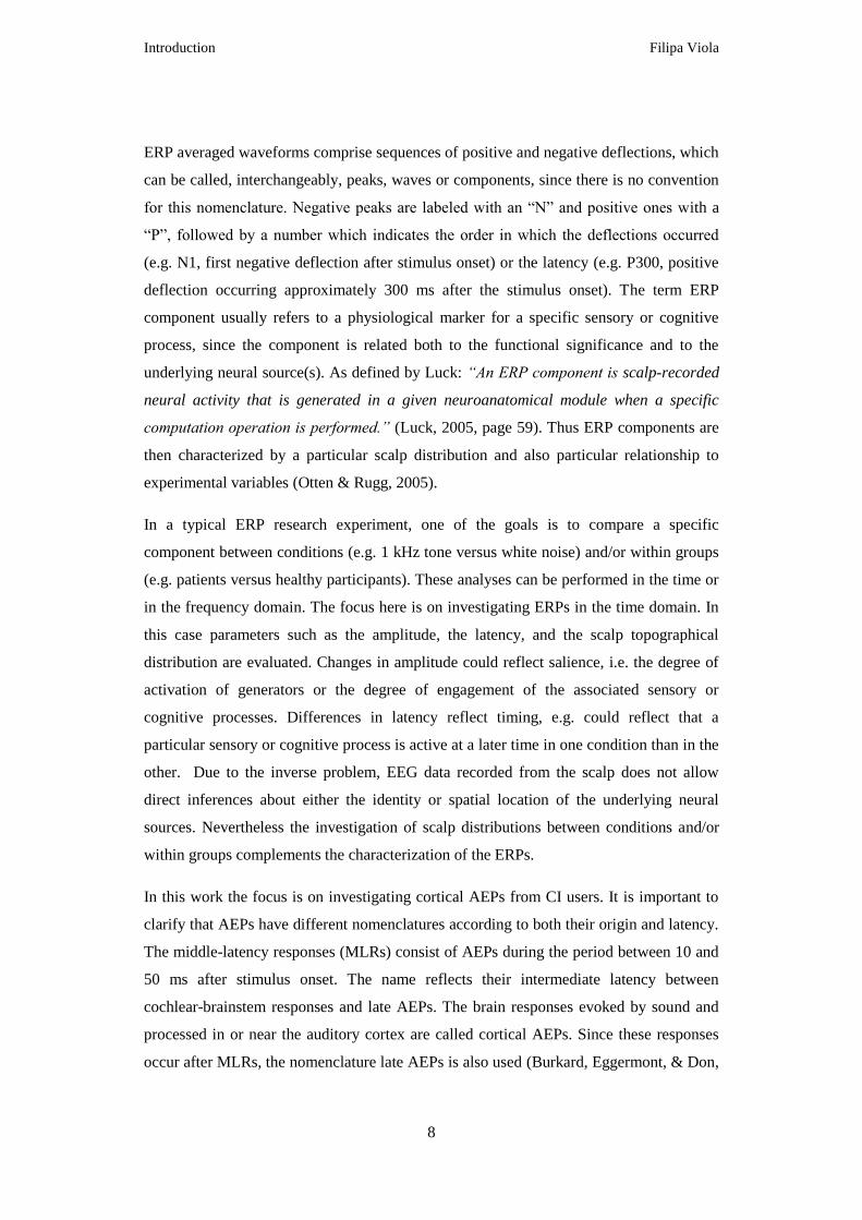
It is known that the amount of noise in an average decreases as a function of the square

root of the number of trials (Luck, 2005, chapter 4). As the ERP model assumes that the

response, i.e. the signal, is unaffected by the averaging process, the SNR increases as a

function of the square root of the number of trials. This mathematical relationship is

illustrated in Figure 2.4. The curves correspond to simulations for different combinations

of measured signal, i.e. ERP response of interest, and noise, i.e. ongoing EEG activity.

For example, in the case of ongoing activity of 50 V and an ERP with amplitude of 5

V, it would be necessary to average 1000 trials to achieve a SNR of approximately 3.

Figure 2.4 Mathematical relationship

between signal-to-noise ratio (SNR)

and number of trials for three

different combinations of signal (S),

i.e. ERP response of interest, and

noise (N), i.e. ongoing EEG activity,

amplitudes ( V).


8

ERP averaged waveforms comprise sequences of positive and negative deflections, which

can be called, interchangeably, peaks, waves or components, since there is no convention

for this nomenclature. Negative peaks are labeled with an “N” and positive ones with a

“P”, followed by a number which indicates the order in which the deflections occurred

(e.g. N1, first negative deflection after stimulus onset) or the latency (e.g. P300, positive

deflection occurring approximately 300 ms after the stimulus onset). The term ERP

component usually refers to a physiological marker for a specific sensory or cognitive

process, since the component is related both to the functional significance and to the

underlying neural source(s). As defined by Luck: “An ERP component is scalp-recorded

neural activity that is generated in a given neuroanatomical module when a specific

computation operation is performed.” (Luck, 2005, page 59). Thus ERP components are

then characterized by a particular scalp distribution and also particular relationship to

experimental variables (Otten & Rugg, 2005).

In a typical ERP research experiment, one of the goals is to compare a specific

component between conditions (e.g. 1 kHz tone versus white noise) and/or within groups

(e.g. patients versus healthy participants). These analyses can be performed in the time or

in the frequency domain. The focus here is on investigating ERPs in the time domain. In

this case parameters such as the amplitude, the latency, and the scalp topographical

distribution are evaluated. Changes in amplitude could reflect salience, i.e. the degree of

activation of generators or the degree of engagement of the associated sensory or

cognitive processes. Differences in latency reflect timing, e.g. could reflect that a

particular sensory or cognitive process is active at a later time in one condition than in the

other. Due to the inverse problem, EEG data recorded from the scalp does not allow

direct inferences about either the identity or spatial location of the underlying neural

sources. Nevertheless the investigation of scalp distributions between conditions and/or

within groups complements the characterization of the ERPs.

In this work the focus is on investigating cortical AEPs from CI users. It is important to

clarify that AEPs have different nomenclatures according to both their origin and latency.

The middle-latency responses (MLRs) consist of AEPs during the period between 10 and

50 ms after stimulus onset. The name reflects their intermediate latency between

cochlear-brainstem responses and late AEPs. The brain responses evoked by sound and

processed in or near the auditory cortex are called cortical AEPs. Since these responses

occur after MLRs, the nomenclature late AEPs is also used (Burkard, Eggermont, & Don,


9

2007). For the sake of simplicity the auditory responses investigated here are referred as

AEPs through this text.

Among other possible classifications AEPs can be divided into two types: exogenous or

endogenous. The former are those whose presence, latency, and amplitude are determined

primarily by the acoustic parameters of the stimulus, and by the integrity of the primary

auditory pathway. The latter have characteristics that vary with the listener’s attention and

performance on assigned cognitive tasks while responses are recorded (reviewed in Cone-

Wesson & Wunderlich, 2003).

Another difference is the type of stimulus that needs to be used to elicit these different

responses. Exogenous AEPs can be elicited both by simple acoustic stimuli such as

clicks, tonebursts, tone-complexes, and by more complex stimuli such as speech or

environmental sounds. These AEPs have three early components labeled P1, N1, and P2,

which reflect sensory encoding of sound that underlies perceptual events (audiologic

applications reviewed in Cone-Wesson & Wunderlich, 2003; Hyde, 1997; Martin,

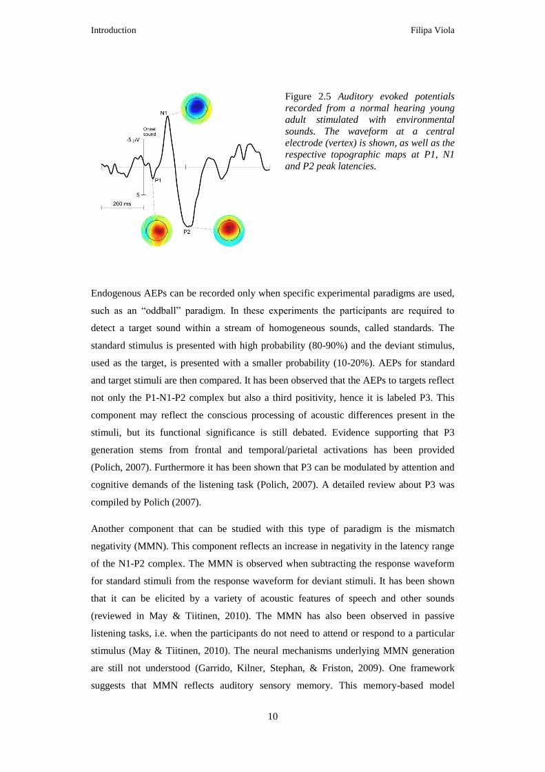
Tremblay, & Korczak, 2008). Figure 2.5 shows a typical P1-N1-P2 complex recorded at a

central electrode (vertex) from a young normal hearing (NH) woman stimulated with

environmental sounds. The topographies at peak latencies are also shown. The

characteristics of the P1-N1-P2 complex are reviewed briefly. P1 is the first positive peak

and occurs approximately 50 ms after stimulus onset. In adults the amplitude of the P1 is

small when compared to the N1-P2 complex, as can be seen in Figure 2.5. In children, on

the other hand, P1 dominates the AEP response and its latency is typically used as a

marker of auditory maturation. The following structures have been reported as neural

generators of P1: primary auditory, hippocampus, planum temporale and lateral temporal

regions (reviewed in Martin, et al., 2008). The negativity following P1 is called N1 and

consists of several distinct subcomponents that peak between 80 and 150 ms (Luck, 2005,

cf. chapter 1). The subcomponent shown in Figure 2.5 is the vertex-maximum potential

that peaks around 100 ms after stimulus onset. N1 has multiple generators located in the

primary and secondary auditory cortex (discussed in detail in Hyde, 1997; Naatanen &

Picton, 1987). The positivity following the N1 is called P2. The morphology of P2 often

covaries with N1 latency and amplitude. Therefore N1 and P2 are sometimes studied

together as the N1-P2 complex. Generators of P2 include both primary and secondary

auditory cortex (reviewed in Martin, et al., 2008).


10

Figure 2.5 Auditory evoked potentials

recorded from a normal hearing young

adult stimulated with environmental

sounds. The waveform at a central

electrode (vertex) is shown, as well as the

respective topographic maps at P1, N1

and P2 peak latencies.

Endogenous AEPs can be recorded only when specific experimental paradigms are used,

such as an “oddball” paradigm. In these experiments the participants are required to

detect a target sound within a stream of homogeneous sounds, called standards. The

standard stimulus is presented with high probability (80-90%) and the deviant stimulus,

used as the target, is presented with a smaller probability (10-20%). AEPs for standard

and target stimuli are then compared. It has been observed that the AEPs to targets reflect

not only the P1-N1-P2 complex but also a third positivity, hence it is labeled P3. This

component may reflect the conscious processing of acoustic differences present in the

stimuli, but its functional significance is still debated. Evidence supporting that P3

generation stems from frontal and temporal/parietal activations has been provided

(Polich, 2007). Furthermore it has been shown that P3 can be modulated by attention and

cognitive demands of the listening task (Polich, 2007). A detailed review about P3 was

compiled by Polich (2007).

Another component that can be studied with this type of paradigm is the mismatch

negativity (MMN). This component reflects an increase in negativity in the latency range

of the N1-P2 complex. The MMN is observed when subtracting the response waveform

for standard stimuli from the response waveform for deviant stimuli. It has been shown

that it can be elicited by a variety of acoustic features of speech and other sounds

(reviewed in May & Tiitinen, 2010). The MMN has also been observed in passive

listening tasks, i.e. when the participants do not need to attend or respond to a particular

stimulus (May & Tiitinen, 2010). The neural mechanisms underlying MMN generation

are still not understood (Garrido, Kilner, Stephan, & Friston, 2009). One framework

suggests that MMN reflects auditory sensory memory. This memory-based model


11

proposes that the MMN indexes preattentive discrimination of a sensory input deviating

from the memory trace formed by the frequent standard stimuli (Naatanen, Gaillard, &

Mantysalo, 1978). The “adaptation model”, in contrary, suggests that the MMN is part

of an amplitude- and latency-modulated N1 response (May & Tiitinen, 2010). The two

models have been reviewed recently by May and Tiitinen (2010).

In this work the focus is on the N1-P2 complex, as these components can be used as an

objective assessment of auditory function (Hyde, 1997). More details about AEPs and

ERPs elicited by stimuli presented in other sensory modalities can be found in specialized

books (Burkard, et al., 2007; Luck, 2005). Guidelines for the preparation of ERP

experiments and for the interpretation of results have been suggested and discussed in the

literature (Kotchoubey, 2006; Luck, 2005; Otten & Rugg, 2005; Picton et al., 2000).

2.1.3. 6BArtifacts in EEG recordings

According to Talsma and Woldorff artifacts can be defined as “… occurrences of any

given electrical activity that can be recorded by EEG equipment, which is not originating

from cerebral sources, and either clearly distinguishable from the recorded background

EEG or substantially large enough to modify the observed ERP waveform from its true

waveform” (Talsma & Woldorff, 2005, page 115).

For the sake of simplicity in this section EEG artifacts are classified in two main

categories: biological and non-biological. The former can be eye blinks or other type of

ocular activity, such as eye movements, muscle artifacts, electrocardiographic (ECG)

activity, or pulse-wave artifacts, caused by the pulsation of an artery near a recording

electrode. The latter can be caused by movement of the electrode wires, instrumentation

artifacts or interference artifacts. Some non-biological artifacts can be minimized by

adopting careful routines in the laboratory before recording EEG data. Sources of noise

and interference for instance should be removed from the room or booth where the

recordings are taking place. Examples are mobile phones, lights, or other unnecessary

electronic equipment. The slow polarization of electrodes, due to perspiration of the

participant, or detachment of the electrodes, can also cause instrumentation artifacts. Thus

the electrodes and the wiring should be checked to confirm that there are no loose

connections. Moreover the impedances of all electrodes should be evaluated before

recording. It is important to make sure that the paste that establishes the connection

between the scalp and the electrodes is not too dry. Furthermore participants should be

instructed to sit still but relaxed during the recording session and not to pull or touch the

electrodes and cables.


12

After the recording session some artifacts can also be attenuated by filtering and

averaging the data. Filtering from 0.01 to 30 or 40 Hz is a typical approach, on the

assumption that in many ERP experiments brain activity of interest is normally in this

frequency range (Luck, 2005, cf. chapter 5). This procedure attenuates or excludes mainly

non-biological artifacts and muscle artifacts. According to the ERP model, averaging

across trials can also attenuate artifacts, as long as these are assumed to be random (see

Figure 2.3). However artifacts are not always random, as is the case for instance with eye

blinks associated with the presentation of visual stimuli. Another example is when a

participant wears an electronic prosthesis such as a CI. The device causes an electrical

artifact that is time-locked to auditory stimuli and cannot be attenuating by filtering or

averaging.

The rejection of portions of EEG data where artifacts occur is also a common approach.

This procedure can be effective in removing eye blinks or other ocular activity, as these

artifacts are not expected to be present in every single trial. Nevertheless the reduction of

the number of trials contributing to the average response reduces the SNR, as described

previously (see Figure 2.4). It is then necessary to record long experiments to ensure that

the number of trials after rejection is still large. This is sometimes not feasible, for

instance when testing children or clinical populations.

In the case of the attenuation of ocular artifacts several regression methods have been

proposed (cf. Croft & Barry, 2000). These approaches require the measurement of the

activity of an extra electrode placed under the eye. This signal is then correlated to the

EEG signal recorded at the scalp. This identifies the artifacts which can then be

subtracted from the data. However it has been suggested that the regression procedures

can cause distortions in the spatial distribution of EEG recordings (Berg & Scherg, 1991).

Thus other techniques such as dipole source modeling, principal component analysis and

independent component analysis (ICA) have been proposed (reviewed in Talsma &

Woldorff, 2005). The next section explains the principles of ICA with a particular focus

on using this method to attenuate artifacts from EEG recordings.

2BIndependent component analysis 2.2.

Independent component analysis (ICA) is a blind source separation technique that

separates complex signals into maximal statistically independent sources (components). It

had its origins in the 1980s and early 90s in France, and has been linked most frequently

to the engineering field (Comon, 1994). Now it is also applied in in the field of human

electro- or magnetographic signals, i.e. electrical and magnetic activity produced by the


13

cells of the human body. ICA has been used with the goal of separating the signal of

interest, e.g. heart or brain activity, from artifact sources. Several studies using ECG (e.g.

Chawla, Verma, & Kumar, 2008), magnetocardiography (MCG) (e.g. DiPietroPaolo,

Muller, Nolte, & Erne, 2006; Muller, Nolte, Paolo, & Erne, 2006), EEG (e.g. Gwin,

Gramann, Makeig, & Ferris, 2010; Jung et al., 2000a; Jung et al., 2000b; Makeig, Jung,

Bell, Ghahremani, & Sejnowski, 1997) , EEG recorded inside a magnetic resonance

imaging (MRI) scanner (e.g. Debener, Mullinger, Niazy, & Bowtell, 2008b; Debener et

al., 2007), and magnetoencephalography (MEG) (e.g. Escudero, Hornero, Abasolo,

Fernandez, & Lopez-Coronado, 2007; Mantini, Franciotti, Romani, & Pizzella, 2008)

have reported that ICA could successfully disentangle different artifacts from brain

sources.

In the case of EEG signals, ICA has been shown to be particularly successful in

attenuating biological artifacts such as eye blinks (e.g. Hoffmann & Falkenstein, 2008;

Jung, et al., 2000a; Jung, et al., 2000b; Mennes, Wouters, Vanrumste, Lagae, & Stiers,

2010), and even movement artifacts during walking and running (Gwin, et al., 2010).

However the applications of ICA in the EEG field are not limited to the attenuation of

artifacts. A number of studies have shown that ICA can also be used to provide insights

about the dynamics of human cortical activity that go beyond the traditional ERP

approach (Debener, Makeig, Delorme, & Engel, 2005a; Debener et al., 2005b; Gramann

et al., 2010; Makeig, Debener, Onton, & Delorme, 2004a; Makeig et al., 2004b; Makeig

et al., 2002; Onton, Westerfield, Townsend, & Makeig, 2006).

There are several ICA algorithms that have been applied to EEG data. Some examples are

infomax (Bell & Sejnowski, 1995), extended-infomax (Lee, Girolami, & Sejnowski,

1999), JADE (Cardoso & Souloumiac, 1994), and fastICA (Hyvarinen & Oja, 2000).

However in the last years the popularity of ICA has increased to the extent that nowadays

there are many more different algorithms suited to different applications. In the online

platform “ICA Central” (http://www.tsi.enst.fr/icacentral/), as of August 2011, there were

27 different ICA algorithms that could be freely downloaded. Some authors have

proposed the implementation of ICA algorithms in the time domain (Makeig, et al., 1997;

Makeig et al., 1999; Makeig, et al., 2002). Other authors have implemented ICA in the

spatial domain, normally in applications to functional magnetic resonance imaging

(fMRI) data, (e.g. Anemuller, Duann, Sejnowski, & Makeig, 2006; McKeown et al.,

1998a; McKeown et al., 1998b). A combination of temporal and spatial ICA has also

been suggested (James & Demanuele, 2010).


14

Comprehensive detailed explanations about ICA can be found in specialized text books

(Comon & Jutten, 2010; Hyvärinen, Karhunen, & Oja, 2001; Stone, 2004). The goal here

is to provide basic information about the mathematical assumptions behind ICA focused

on its application to the processing of EEG signals (2.2.1). Section 2.2.2 describes the

application of temporal ICA to the attenuation of artifacts from EEG data using the

extended-infomax algorithm as implemented in the EEGLAB toolbox (Delorme &

Makeig, 2004) running in the MATLAB (Mathworks, Natick, MA) environment. Lastly

the practical problems associated with this attenuation procedure are described, and

improvements are suggested (2.2.3).

2.2.1. 7BApplication to EEG data

In the late 90s ICA was applied with success for the first time to a set of EEG data

(Makeig, et al., 1997). Nevertheless the application of ICA requires that various

assumptions are considered. The implementation described here considers that the

number of sensors and sources are the same, and is called a “complete” decomposition

method. However it is not possible to know how many independent sources contribute to

the EEG signal. Another a priori obvious pre-requisite is that the signal of interest needs

to be a linear mixture of different sources that are assumed to be independent and

summed linearly at the sensors. Additionally it is assumed that there are no differential

delays involved in projecting the source signals to the different sensors. A further

assumption is that the component source locations (and thereby their topographic

projection patterns to the scalp sensors) are fixed throughout the data.

These assumptions are quite plausible for EEG data, as illustrated in Figure 2.6.

Regarding the assumption of temporally independence of the sources, as long as two

sources are not perfectly coupled during the recording, they may express some degree of

temporal independence. This amount of partial independence (or partial connectivity)

may be sufficient for ICA to achieve a good degree of unmixing (Debener, Thorne,

Schneider, & Viola, 2010). The assumption that each signal is a linear mixture of source

signals is quite plausible for electrical signals travelling through human tissue, as well as

the assumption that any delay is negligible (Stone, 2004). Since most neural signals

picked up by EEG are generated by PNs, it is also reasonable to assume that in the

absence of movement of electrodes, the component source locations are fixed throughout

the data (Debener, et al., 2010).

Another assumption that also needs to be met when applying ICA is that the probability

distributions of the individual component source activity values are not precisely


15

Gaussian, which is important to ensure the independence of sources. This assumption is

plausible for EEG sources generated by nonlinear cortical dynamics as well as for non-

brain artifact sources including cardiac signals, line noise, muscle signals, eye blinks and

eye movements (Makeig & Onton, 2011).

Figure 2.6 ICA assumptions applied to EEG data. ICA identifies (A) temporally distinct

(independent) signals generated by partial synchronization of local field potentials within

cortical patches (B). The resulting far-field potentials summed (Σ), in differing linear

combinations, at each electrode depending on the distance and orientation of each

cortical patch generator relative to the (A) recording and (C) reference electrodes

(adapted from Onton & Makeig, 2009).

It seems that there is an approximate fit between ICA assumptions and the physiological

nature of EEG sources. Nevertheless it is important to highlight that exact independence

is such a strict requirement that it can never be established for EEG signals with finite

length. ICA algorithms, therefore, may at best produce components with maximal

independence by ensuring that components continually approach independence as the

ICA algorithm is iteratively applied to the data. The degree of IC independence achieved

may differ for different data sets and also for different ICA algorithms applied to the

same dataset (Makeig & Onton, 2011).

The different ICA algorithms need to provide a measure of independence. However

independence cannot be measured directly, and other quantities that are related to

independence need to be considered. In the case of the infomax type algorithms, infomax

(Bell & Sejnowski, 1995) and extended-infomax (Lee, et al., 1999), the measure adopted

is entropy. Entropy is defined as a measure of the uniformity of a distribution of a

bounded set of values, such that complete uniformity corresponds to maximum entropy.

Variables with maximum entropy are statistically independent of each other (Stone,


16

2004). The infomax approach consists in finding an unmixing matrix that maximizes the

entropy of the signals extracted by that matrix. This unmixing matrix will also maximize

the amount of mutual information between the signals and the set of signal mixtures,

hence the name infomax (Stone, 2004).

Figure 2.7 shows a schematic outline illustrating the application of ICA to EEG data. The

EEG raw data (Scalp Data) can be defined as a matrix X (channels x time). The ICA

decomposition finds an unmixing matrix W which, when multiplied by X, decomposes the

data into a matrix of independent component signals, called the independent component

(IC) activations matrix A (right). Please note that the number of ICs is determined by the

number of EEG channels recorded (“complete” decomposition). Multiplying the IC

activations matrix by the inverse of the unmixing matrix, also called mixing matrix W-1

(middle) reconstitutes or back-projects the original scalp data channels. The columns of

the mixing matrix give the relative strengths and polarities of the projections of one IC to

each of the scalp channels. This representation is normally called IC scalp maps or IC

topographic maps. By setting a particular row from the activations matrix to zero it is

possible to eliminate the contribution of that particular IC to the raw data when back-

projecting, as discussed in the next section.

Figure 2.7 Schematic outline illustrating the application of ICA to multi-channel EEG

data (X).Inverse weights (W-1) represent the spatial pattern of each source time course.

Matrix-multiplication of W-1 with the maximally temporally independent time courses (in

A) gives the mixed channel data, a process called back-projection. For illustration

purposes, one component/channel vector is highlighted in grey and shown below the

corresponding matrices (from Debener, et al., 2010).

When comparing IC activations and scalp maps it is also important to keep in mind that

when evaluating both sets of information separately there will be an inherent ambiguity in

terms of polarity and amplitude. This occurs because the sign and scaling of the back-


17

projected IC in the data is split arbitrarily between its activation and scalp map. Using a

numeric example, since -1 × -1 = 1, inverting the signs of both an IC activation and its

scalp map will not change their product, or the back-projection of the IC into the original

data, which will retain its original polarity (Makeig & Onton, 2011). Moreover it is

important to keep in mind that infomax based-ICA can produce different results from

repeated application to identical data. This results from the unmixing weights (W) being

learned over repeated iterations, which use randomly chosen samples from the training

data submitted (X) (Debener, et al., 2010).

A major contribution that has made ICA popular among EEG/ERP laboratories all over

the world was the development of a MATLAB (Mathworks, Natick, MA) open source

toolbox called EEGLAB (Delorme & Makeig, 2004). The functions contained in the

EEGLAB toolbox can be run from a graphical user interface or in scripts, making it a

suitable tool both for novices and experienced researchers. In the last years ICA

algorithms have also been implemented in many commercial software packages used for

the recording and processing of EEG data. Details about applying ICA to attenuate

artifacts from EEG recordings using EEGLAB are discussed in the next section.

2.2.2. 8BEEG artifact attenuation

The quality of an ICA decomposition depends mainly on the quality of the EEG training

data submitted to the ICA algorithm. Consequently the degree of artifact attenuation that

can be achieved depends also on the quality of the decomposition, which can be

substantially influenced by the pre-processing of the data, e.g. filtering. Practical

guidelines for decomposing multi-channel EEG data and evaluating ICs have been

covered by several authors (Debener, et al., 2010; Makeig & Onton, 2011; Onton, et al.,

2006). An important aspect is that the ICA algorithm should be trained using sufficient

data points from the n-channels recorded. It has been proposed that the number of points

should be at least a k multiple of n2, being recommend that k should not be smaller than

20 (Debener, et al., 2010; Onton, et al., 2006). However “quantity” and “quality” are both

important in this respect. The “quality” of the data can be substantially improved by using

appropriate filters (cf. Debener, et al., 2010) and also by removing from the data portions

containing non-stereotyped artifacts, such as movements arising from the pulling of

cables or electrodes. Sometimes it can be necessary to remove bad channels, i.e. those

electrodes which have lost good contact to the scalp, from the raw data matrix before

running ICA. In summary the pruning of the data is highly recommended, since these

types of artifacts can introduce many different unique and independent scalp maps in the

recorded data, i.e. fewer ICs will be available to represent other processes of interest


18

(Onton, et al., 2006). The EEGLAB toolbox contains implementations of several

detection methods that can automatically identify trials containing non-stereotyped

artifacts (Delorme, Sejnowski, & Makeig, 2007a).

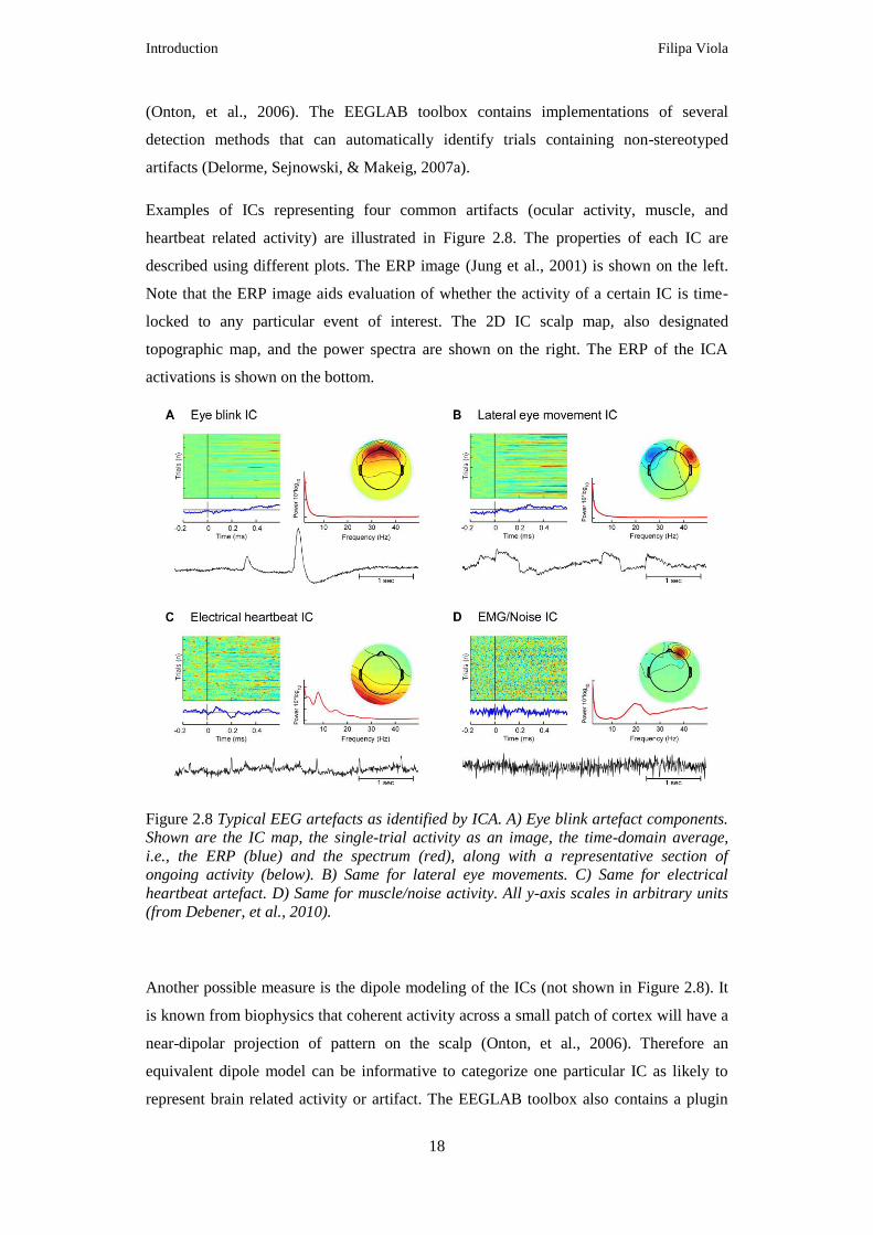
Examples of ICs representing four common artifacts (ocular activity, muscle, and

heartbeat related activity) are illustrated in Figure 2.8. The properties of each IC are

described using different plots. The ERP image (Jung et al., 2001) is shown on the left.

Note that the ERP image aids evaluation of whether the activity of a certain IC is time-

locked to any particular event of interest. The 2D IC scalp map, also designated

topographic map, and the power spectra are shown on the right. The ERP of the ICA

activations is shown on the bottom.

Figure 2.8 Typical EEG artefacts as identified by ICA. A) Eye blink artefact components.

Shown are the IC map, the single-trial activity as an image, the time-domain average,

i.e., the ERP (blue) and the spectrum (red), along with a representative section of

ongoing activity (below). B) Same for lateral eye movements. C) Same for electrical

heartbeat artefact. D) Same for muscle/noise activity. All y-axis scales in arbitrary units

(from Debener, et al., 2010).

Another possible measure is the dipole modeling of the ICs (not shown in Figure 2.8). It

is known from biophysics that coherent activity across a small patch of cortex will have a

near-dipolar projection of pattern on the scalp (Onton, et al., 2006). Therefore an

equivalent dipole model can be informative to categorize one particular IC as likely to

represent brain related activity or artifact. The EEGLAB toolbox also contains a plugin


19

toolbox called DIPFIT that allows the dipole modeling of ICs (Oostenveld & Oostendorp,

2002). More details about how to interpret the results of dipole modeling of ICs can be

found in the literature (Gramann, et al., 2010; Makeig & Onton, 2011; Onton, et al.,

2006).

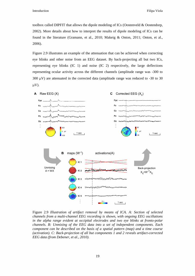
Figure 2.9 illustrates an example of the attenuation that can be achieved when correcting

eye blinks and other noise from an EEG dataset. By back-projecting all but two ICs,

representing eye blinks (IC 1) and noise (IC 2) respectively, the large deflections

representing ocular activity across the different channels (amplitude range was -300 to

300 V) are attenuated in the corrected data (amplitude range was reduced to -30 to 30

V).

Figure 2.9 Illustration of artifact removal by means of ICA. A: Section of selected

channels from a multi-channel EEG recording is shown, with ongoing EEG oscillations

in the alpha range evident at occipital electrodes and two eye blinks at fronto-polar

channels. B: Unmixing of the EEG data into a set of independent components. Each

component can be described on the basis of a spatial pattern (map) and a time course

(activation). C: Back-projection of all but components 1 and 2 reveals artifact-corrected

EEG data (from Debener, et al., 2010).


20

Although the underlying mathematical formulations of ICA are complex, its application

to EEG data is well described. Nevertheless the use of ICA requires dealing with some

practical challenges. For instance, the larger the number of EEG channels available, the

larger the number of ICs that need to be evaluated and the more likely that a particular

type of artifact will be represented in more than one IC. In the next section the selection

of ICs is described and possible improvements are suggested.

2.2.3. 9BPractical problems

Several studies have shown that the attenuation of different types of artifacts can be

successfully achieved using ICA (e.g. Debener, et al., 2007; Jung, et al., 2000a; Jung, et

al., 2000b). It has been shown that even more complex artifacts such as stimulus-locked

electrical artifacts from CIs can be attenuated (e.g. Debener, Hine, Bleeck, & Eyles,

2008a; Gilley et al., 2006). Details about this particular type of artifact will be discussed

in a dedicated section (2.3.4.).

In practical terms, the procedure of screening and selecting ICs representing artifacts

relies mainly on visual inspection of the properties of the ICs. This method is time

consuming, since all ICs from all participants need to be evaluated. For example, in an

experiment where 20 participants are measured with a 32 channels EEG system, a total of

640 (20x32) ICs would need to be screened. However the total number of ICs in an EEG

study can be even larger because nowadays many laboratories use high-density EEG

recordings with more than 60 channels. Moreover the screening procedure requires

expert knowledge and training. Therefore questions about the subjectivity associated with

the procedure of selecting ICs have been raised.

The EEGLAB toolbox contains special functions that allow the clustering of ICs across

datasets from different participants, using clustering algorithms based on measures of the

Mahalanobis distance or on a neural network approach. This clustering procedure relies

on a multiple-measure approach where the user needs to set combinations of different

parameters, i.e. weights for each measure. This approach has been used to cluster ICs

related to distinct brain processes (e.g. Gramann, et al., 2010). On the other hand, due to

the special properties of ICs related to some particular artifacts, it could be possible to

implement procedures based on a single measure. One particular example is the eye blink

artifact. It has been observed that ICs representing this artifact have very similar scalp

maps across different participants, which can be assumed to be highly correlated. This

results from the fact that the eyes, the source of the artifact, have a fixed position relative

to the EEG electrodes. Due to the rising popularity of ICA, especially in attenuating


21

biological artifacts in EEG data, it would be of interest to develop user friendly

approaches, targeted at identifying specific ICs.

Another important question concerns the evaluation of the stability and reliability of an

ICA decomposition. As described previously, due to the iterative learning procedure of

the unmixing matrix, ICA can produce different results from repeated applications to

identical data (cf. Debener, et al., 2010). A method for ICA reliability analysis based on

clustering and visualization has been proposed (ICASSO, described in Himberg,

Hyvarinen, & Esposito, 2004). Recently other approaches have been suggested (Debener,

et al., 2010; Groppe, Makeig, & Kutas, 2009). Some authors have proposed a method

where ICA is applied separately to split-halves of a data, as well as for the whole data.

Reliability is checked by evaluating IC triplets (Groppe, et al., 2009). Other authors have

applied ICA twice to identical data, and correlated the weights from the first and second

applications to identify maximum correlations for each IC. With this procedure it was

possible to compare ICA decompositions obtained using different amounts of training

data (Debener, et al., 2010).

3BAssessment of auditory evoked potentials in cochlear implant users 2.3.

A cochlear implant (CI) is a neural prosthesis that uses electrical stimulation to enhance

or restore auditory function in particular cases of hearing impairment. From

conceptualization to the latest developments in CI technology it has been a journey of

more than two centuries. Figure 2.10 shows a time line illustrating the main achievements

in CI technology. An impressive single figure summarizes the success of these

milestones: more than 220,000 individuals have been implanted with CIs worldwide

(Cosetti & Waltzman, 2011).

This section is focused on the assessment of auditory cortical functions of CI users by

means of AEPs, an objective measurement of auditory rehabilitation. First a brief

introduction to the functioning of the healthy auditory system is presented (2.3.1),

followed by the description of common causes of deafness, as well as available

treatments with a particular focus on the CI technology (2.3.2). The components and

working mode of a modern CI are described, as well as common clinical measurements

used to evaluate auditory rehabilitation after the device is switched on (2.3.3). A

particular emphasis is given to the use of EEG as a non-invasive technique to measure

AEPs from CI users and investigate objectively auditory rehabilitation after implantation

(2.3.4). Recent findings from studies that have used AEPs to study CI populations are

briefly described. Lastly the challenges associated with the artifacts caused by the CI


22

device in the EEG recordings are presented and current solutions to overcome this

problem are discussed (2.3.5).

Figure 2.10 Three phases defining the major events in the development of CIs. The

conceptualization phase demonstrated the feasibility of electric stimulation. The research

and development phase legitimized the utility and safety of electric stimulation. The

commercialization phase saw a wide-spread use of electric stimulation in treating

sensorineural hearing loss (from Zeng, Rebscher, Harrison, Sun, & Feng, 2008).

2.3.1. 10BThe human auditory system

The human auditory system consists of the ear itself, which comprises three specialized

regions, the outer, the middle, and the inner ear (Figure 2.11) plus the auditory pathways

of the brain. Each region of the ear has a different function which allows sound waves

travelling through the air to be converted to neural activity. The auditory pathways of the

brain comprise different brain structures, in particular the brainstem, the pons, the

midbrain, the thalamus, and the auditory cortex (Figure 2.12). A brief description of the

mechanisms of hearing is provided here, with a special focus on the functioning of the

cochlea. A detailed explanation of the auditory pathways is out of the scope of this work.

This information can be found in specialized text books (Burkard, et al., 2007;

Rosenzweig, Breedlove, Leiman, & Watson, 2005; Winer & Schreiner, 2010).


23

Figure 2.11 Anatomy of the peripheral auditory system. Diagrammatic cross-section

through the human head illustrating the three (outer, middle and inner) regions of the

ear. The outer ear is comprised of the pinna and external auditory meatus, and is

bounded on its medial side by the tympanic membrane. The middle ear is an air-filled

space containing the three auditory ossicles bounded by the tympanic membrane as well

as the round and oval windows. The inner ear is comprised of the cochlea, a membranous

labyrinth (blue), which is surrounded by a bony labyrinth and innervated by the VIIIth

(statoacoustic) cranial nerve (green) (adapted from Kelley, 2006).

In a healthy hearing system the sound waves traveling through air are captured and

filtered by the pinna in the outer ear. These waves reach the tympanic membrane via the

ear canal, and cause vibrations that move a chain of ossicles in the middle ear. This action

produces a piston–like movement and causes the tilting of the oval window that is a

flexible membrane that separates the middle from the inner ear. The cochlea is part of the

inner ear, and can be described as a membranous labyrinth. As the cochlea is filled with

noncompressible fluid, the vibrational energy generated in the middle ear can be

converted into waves of fluid. One of the complex structures of the cochlea is the basilar

membrane. This structure divides the cochlea along its length, and vibrates producing the

phenomenon of traveling waves. Furthermore it contains the organ of Corti that is the

principal structure involved in converting these waves into neural activity. The organ of

Corti contains specialized hair cells: the outer hair cells (OHC) and the inner hair cells

(IHC). The OHC, the cells with active mechanical behavior, amplify sound by up to 60

decibels (dB) and provide superior frequency selectivity. This is of particular benefit for

humans, because it enables sophisticated speech and music perception. The IHC, the

sensory cells, sense the movement of the basilar membrane and deflect accordingly. This

initiates a chain of electrochemical events that causes electrical spikes, or action


24

potentials. The electrical currents are in turn transmitted to the brain via the auditory

nerve and the auditory pathways.

Figure 2.12 Auditory pathways of the human brain. This view from the front of the head

shows the first binaural afferent interactions in the brainstem. Most (but not all) of the

information from each ear projects to the cortex on the opposite side of the brain, as

illustrated here by the colors of the projections to the medial geniculate nucleus and

cortex (from Rosenzweig, et al., 2005).

Many events can disturb the normal functioning of the auditory system and even impair it

permanently. One unavoidable example is age related hearing loss (ARHL) or

presbyacusis which is related to functional loss of sensory and neural elements. It is

known that hearing acuity declines with age. The high frequencies are affected first,

followed by the frequencies of the speech spectrum (Roth, Hanebuth, & Probst, 2011).

ARHL is the most widespread sensory impairment in aging people, and as it is a

progressive condition, a formal diagnosis can sometimes only be provided at later stages.

The next section describes types of hearing loss, etiologies and available treatments.

2.3.2. 11BDeafness: etiologies and treatments

According to the World Health Organization (WHO), deafness and its causes can be

defined as the following: “Deafness is the complete loss of the ability to hear from one or

both ears. Deafness may be inherited, or caused by complications at birth, certain

infectious diseases, such as meningitis, use of ototoxic drugs, and exposure to excessive


25

noise”. The term hearing impairment is also commonly used and refers to partial or

complete loss of the ability to hear. Deafness can be categorized in three types, according

to which part of the hearing system is affected (Rosenzweig, et al., 2005).

The first type is conduction hearing loss and is related to disorders of the outer or middle

ear. In this pathology the vibrations produced by the auditory stimuli are prevented from

reaching the cochlea. The second type is sensorineural hearing loss (SNHL), which

occurs when OHC and/or IHC are impaired, as illustrated in Figure 2.13. The OHC

appear to be especially susceptible to noise trauma. Other causes for SNHL include

genetic defects and treatments with ototoxic antibiotics. The third type of deafness is less

common and is called central hearing loss. This pathology is caused by lesions in the

auditory pathways or in the primary auditory cortex, hence sometimes also called

“cortical deafness”. This type of deafness has been investigated mainly in single case

reports (Hood, Berlin, & Allen, 1994; Kaga, Nakamura, Takayama, & Momose, 2004).

Figure 2.13 Illustration of sensorineural hearing loss. This type of impairment is caused

by damage to or destruction of hair cells and may also involve the deterioration of neural

connections in the inner ear. In normal hearing, OHC along the basilar membrane detect

sound vibrations. In response, IHC release chemical transmitters that trigger action

potentials in neurons of the spiral ganglion. The patterns of evoked neural activity convey

information to the central nervous system (top). In a profoundly deafened ear, IHC have

died or no longer function, depriving the spiral ganglion cells of their normal input

(bottom). Without regular use, the neural connections often wither and some cells of the

spiral ganglion may die. For the sake of simplicity, this diagram does not reflect

anatomical details or consistent scale (from Dorman & Wilson, 2004).


26

According to WHO, solutions to hearing impairment should start with a focus on

prevention and on early detection. It has been estimated that around half of all deafness

and hearing impairment could be prevented (cf. WHO website: www.who.int). In the case

of conduction hearing loss common treatments are the prescription of hearing aids or

middle ear implants. The former provide sound amplification, increasing the movement

of the eardrum and promoting indirectly the vibration in the middle ear. The latter

enhance the signal that reaches the inner ear by directly vibrating the middle ear

structures while leaving the ear canal open and the eardrum undisturbed. In the case of

SNHL, when the only affected cells are the OHC, auditory function can be restored by

means of hearing aids that provide powerful amplification. When the IHC are also

damaged the prescribed treatment is a CI. These patients are clinically defined as

profoundly deaf. These individuals can have a loss of more than 100 dB, so they cannot

hear for instance the sound of an airplane flying close by. Treatment with a CI is only

possible when the electrical excitability of the auditory nerve fibers remains intact. When

the auditory nerve is damaged a solution is to use another device called a brainstem

implant. In this case the electrical stimulation is delivered directly to the brainstem, more

specifically to the cochlear nucleus. Figure 2.14 illustrates available treatments for

conduction and SNHL in the form of medical devices such as hearing aids, middle ear

implants, cochlear implants, and brainstem implants.

Figure 2.14 Treatment of hearing impairment using hearing aids, middle ear implants,

cochlear implants, and brainstem implants (from Zeng, et al., 2008).

http://www.who.int/


27

2.3.3. 12BRestoration of auditory function with cochlear implants

In this section the general functioning of modern CIs, and the outcomes after cochlear

implantation are described. Additionally typical clinical measurements of auditory

rehabilitation are discussed. The first successful attempt to stimulate electrically totally

deafened individuals dates to 1957, when a French physician and a French engineer,

Djourno and Eyries, placed a coil of wire in the inner ear of two patients, who then

reported some hearing (Moore & Shannon, 2009; Zeng, et al., 2008). This observation

was replicated a few years later in the USA by William House in Los Angeles and by

Blair Simmons in Stanford. In the following years fruitful research was conducted in

multiple centers (for more details see Zeng, et al., 2008). But only in 1984 did the

3M/House device, a single electrode implant, gain Food and Drug Administration (FDA)

approval in the USA. One year later the first FDA approved multi-channel device, the

Nucleus 22, became available on the market. This device had 22 channels, being the

precursor of the CI technology used nowadays. Currently there are devices on the market

from four different manufacturers. The studies available in the literature do not show

evidence of any specific device being superior to the others (Cosetti & Waltzman, 2011).

A detailed comparison of CI technology among the different manufacturers is beyond the

scope of this work but can be found in the literature (Cosetti & Waltzman, 2011; Wilson

& Dorman, 2008b; Zeng, et al., 2008).

The general principle of a modern CI is to mimic the function of the healthy cochlea by

delivering artificial electrical stimulation to the auditory nerve and thereby allowing the

restoration of auditory function. These devices comprise external and internal

components which are described briefly. As shown in Figure 2.15, the behind-the-ear

external processor consists of four parts. There is a battery pack, a microphone, a speech

processor, and an external transmitter, which includes an antenna. The microphone

captures the sound in the environment and the speech processor transforms the

microphone output into a digital signal. This digital signal is processed and encoded into

a radio frequency (RF) signal, which is sent to the antenna. The external transmitter then

provides a transcutaneous link for the transmission of power and stimulus information

across the skin. (Wilson & Dorman, 2008a, 2008b; Zeng, et al., 2008).

Internally the CI consists of an implanted receiver/stimulator, and an array of electrodes

(Figure 2.15). The receiver/stimulator decodes the information received from the RF

signal and converts it into electrical currents. These currents are then sent along wires to

the intra-cochlear electrodes, which at the end of the wire stimulate the auditory nerve

directly. Several parameters need to be taken into account when providing the


28

stimulation, for instance the distance between electrodes and the depth of insertion. Since

the goal is to mimic the tonotopic organization of the cochlea the stimulation needs to be

provided to distinct sites. Nowadays the array comprises between eight and twenty two

electrodes, but not all of them are active at the same time. The configuration of active

electrodes is personalized for the user during the fitting session where the CI is switched-

on.

Figure 2.15 Components of modern cochlear implant systems. A microphone, a battery

pack, and a speech processor are incorporated into the behind-the-ear (BTE) housing in

the illustrated system, much like BTEs of hearing aids. A thin cable connects the output of

the speech processor (transmitting a radio frequency signal with encoded stimulus

information) to the external transmitting coil that is positioned opposite the implanted

receiver/stimulator. The transmitting coil is held in place with a pair of magnets, one in

the center of the coil and another in the implanted receiver/stimulator. The

receiver/stimulator is implanted in a flattened or recessed portion of the skull, posterior

to and slightly above the pinna. The reference (or “ground”) electrode is implanted at a

location remote from the cochlea, usually in the temporalis muscle. For some implant

systems, a metallic band around outside of the receiver/stimulator package serves as

reference electrode. An array of active electrodes is inserted into the scala tympani

through the round window membrane or through a larger drilled opening in the bony

shell of cochlea (cochleostomy) near the round window (from Wilson & Dorman, 2008b).

A significant achievement in CI technology has been the miniaturization of the external

sound processor. The development of the coding strategies, also known as speech

strategies, has also been crucial for the success of the CI technology. These strategies


29

consist of algorithms that are responsible for decomposing the input audio signal into

different frequency bands or channels and delivering the most appropriate stimulation

pattern to the electrodes. Current implementations use a filter bank or waveform approach

(Rubinstein, 2004). Important aspects for this signal transformation are the

implementation of temporal coding and the imitation of the tonotopic organization of the

cochlea. The encoding of spectral and temporal fine structure cues has also received

special attention (Zeng, et al., 2008). Advances in the encoding of these stimulus

properties could contribute to the improvement of speech perception in noise, music

appreciation, and recognition of emotions, which are still a challenge for many CI users

(Cosetti & Waltzman, 2011). Details about the different strategies, their evolution, as well

as advantages and disadvantages are out of the scope of this work and have been

described in the literature (Wilson & Dorman, 2008b; Zeng, et al., 2008).

It is noteworthy that successful encoding of sounds requires not only developments in the

encoding strategies, but also in the intra-cochlear electrode array arrangement and mode

of operation. Other challenges include providing longer lasting batteries and improving

the microphone technology. For instance the use of directional microphones could

contribute to improvements (Cosetti & Waltzman, 2011). Recent developments and

future improvements in CI technology, as well as safety concerns, have been discussed in

the literature (Cosetti & Waltzman, 2011; Wilson & Dorman, 2008a, 2008b; Zeng, et al.,

2008).

Although CI technology has dramatically improved in the last 30 years, the outcome after

implantation is still variable across CI users. Several authors have suggested that the

auditory cortex and its capacity for cortical plasticity should be regarded as an “extra CI

component”. This “biological component” may have a crucial role, since it needs to adapt

to the artificial electrical stimulation in order to allow the restoration of the hearing

function (Moore & Shannon, 2009; Wilson & Dorman, 2008a).

In the last years the implantation candidacy criteria have been broadened to such an

extent that the age of CI users nowadays ranges from children under one year old (Cosetti

& Roland, 2010) to elderly patients implanted after their 70th birthday or later (e.g.

Carlson et al., 2010; Chatelin et al., 2004; Williamson, Pytynia, Oghalai, & Vrabec,

2009). Prelingually deafened adolescents and adults were once considered poor

candidates for cochlear implantation. However nowadays these patients use CIs, and

several assessment studies have been performed after implantation (Most, Shrem, &

Duvdevani, 2010; Santarelli, De Filippi, Genovese, & Arslan, 2008).


30

The main goal in CI technology is to develop devices that allow users to be able to

understand speech and communicate with other people. Therefore the assessment of

outcome after implantation has been based on tests that evaluate speech recognition, and

on questionnaires such as the Abbreviated Profile of Hearing Aid Benefit (Cox &

Alexander, 1995). There are multiple versions of speech recognition tests. These tests can

comprise recognition of phonemes, words or sentences. Results from different speech

recognition tests are summarized in Figure 2.16 (Gifford, Shallop, & Peterson, 2008).

The stimulation can be delivered in silence or in noisy conditions, with or without visual

cues, and with or without the use of hearing aids. The scores are normally calculated as

the percent (%) of correct phonemes or words repeated by the CI user. For tests

performed in noise, the score is typically a speech recognition threshold measured in dB

that corresponds to the SNR at which 50% of the speech material is recognized correctly.

In Figure 2.16 it can be observed that for test A, the Hearing in Noise Test (HINT) with

sentences in quiet, a large number of CI users scored above 90%. On the other hand, for

test D, the Bamford-Kowal-Bench Speech-in-Noise (BKB-SIN), a large variability in

performance was observed across CI users.

Figure 2.16 Individual subject performance for the Hearing in Noise Test (HINT) with

sentences in quiet (A; n = 188), the Consonant-nucleus-consonant (CNC) monosyllables

test (B; n =287), AzBio sentences in quiet (C; n = 137), and Bamford-Kowal-Bench

Speech-in-Noise (BKB-SIN) test (D; n = 231) (from Gifford, et al., 2008).

Other authors have also shown that speech recognition tests in quiet can be prone to

ceiling effects, i.e. many adult CI users can achieve scores of 100% (Gifford, et al.,


31

2008). This reflects that with current CI technology for the majority of CI users it is not

difficult to communicate in quiet environments. However, when CI users are assessed

with speech-in-noise tests, the scores tend to be lower, and the large variability of

outcomes across subjects becomes evident (Donaldson et al., 2009; Gifford, et al., 2008;

Wilson & Dorman, 2008a). It is also noteworthy that speech scores are frequently used to

categorize CI users in terms of their performance with the CI.

It seems that parameters such as age at implantation, duration of deafness, exposure to

oral communication and pre-operative hearing thresholds condition the outcome (Cosetti

& Waltzman, 2011). In the case of children, age of implantation seems to be crucial, since

an earlier implantation favors the normal development of auditory functions (Sharma,

Dorman, & Kral, 2005; Sharma, Dorman, & Spahr, 2002) and acquisition of language

(Peterson, Pisoni, & Miyamoto, 2010; Uhler, Yoshinaga-Itano, Gabbard, Rothpletz, &

Jenkins, 2011). In the case of post-lingually adults, the duration of deafness seems to be a

key parameter. It is likely that these deafened individuals can associate the new artificial

stimulation patterns provided by the implant to their memories of what speech should

sound like (Dorman & Wilson, 2004). In the case of pre-lingually deafened not only does

the duration of deafness seems to be important, but also the exposure to oral

communication (Cosetti & Waltzman, 2011). However it is not always easy to establish

the onset of deafness for each patient. As mentioned previously, deafness is frequently a

progressive condition and formal diagnosis can sometimes only be provided at later

stages.

In order to better investigate outcomes after implantation, it has been suggested that CI

users should be assessed with a battery of tests, instead of a single test (Gifford, et al.,

2008). Moreover it is also important to establish recommendations and guidelines for the

use of the different speech recognition tests. This may ensure that the interpretation of the

results across clinics would provide unbiased, objective measurement of auditory

rehabilitation (Theunissen, Swanepoel de, & Hanekom, 2009). On the other hand a

number of authors have argued that AEPs can be a valuable measurement to objectively

evaluate auditory rehabilitation (e.g. Brix & Gedlicka, 1991; Cone-Wesson &

Wunderlich, 2003; Kraus et al., 1993; Shallop, 1993), especially when dealing with

prelingually deafened CI users (McNeill, Sharma, & Purdy, 2009) or pediatric

populations (Kileny, 2007; Singh, Liasis, Rajput, Towell, & Luxon, 2004).


32

2.3.4. 13BAuditory evoked potentials as an objective assessment of auditory

rehabilitation

Evidence of plasticity in the auditory cortex of adult post-lingually deafened CI users has

been reported in a longitudinal MEG study, where it was shown that the auditory cortex

of CI users could adapt to the artificial stimulation within just the first six months

(Pantev, Dinnesen, Ross, Wollbrink, & Knief, 2006). However it is still not yet well

understood how either the adaptation process itself or any deficits of adaptation could

relate to the large variability of outcomes observed after implantation. Furthermore only a

few studies have investigated which parameters can be used as best predictors of

outcome after implantation (van Dijk et al., 1999) and it is still not yet clear which

rehabilitation strategies can contribute to improved performance with the CI (Champoux,

Lepore, Gagne, & Theoret, 2009; Rouger et al., 2007). In the last years, due to its

objectivity and feasibility, AEPs have become a popular technique to investigate how the

auditory cortex from patients adapts to the artificial input delivered by the implant.

Evidence has been provided that electrophysiological responses could be related to

clinical parameters, such as duration of deafness (Kelly, Purdy, & Thorne, 2005;

Sandmann et al., 2010), experience with the implant (Kelly, et al., 2005), or performance

in speech recognition tests (Kelly, et al., 2005; Zhang et al., 2011).

Tables 2.1 and 2.2 list a summary of representative AEP studies with adult CI users, and

implanted children, respectively. The selected studies comprise different research

settings, including different experimental paradigms, EEG montages, and signal

processing tools to attenuate CI artifacts. Studies published before 2002 are not included

in the tables due to space limitations (e.g. Brix & Gedlicka, 1991; Hoth, 1998; Kileny,

Boerst, & Zwolan, 1997; Kraus, et al., 1993; Kubo et al., 2001; Shallop, 1993).

Furthermore, note that AEP studies where the auditory stimulation was delivered directly

to the CI electrodes are also not listed in the tables. (e.g. Guiraud et al., 2007; Makhdoum,

Groenen, Snik, & van den Broek, 1998).

Among the studies with adults, several have investigated the relationship of AEPs to

speech perception (Henkin et al., 2009; Kelly et al., 2005; Lonka et al., 2004; Zhang et

al., 2010; Zhang et al., 2011) or to music perception (Koelsch, Wittfoth, Wolf, Muller, &

Hahne, 2004; Sandmann, et al., 2010). Other authors have investigated brain asymmetries

in the auditory cortex of adult CI users (Debener, et al., 2008a; Sandmann et al., 2009).

Outcomes of these studies have revealed relationships between AEPs and clinical

profiles. For instance shorter P2 latencies were associated with higher speech recognition

scores and shorter durations of deafness (Kelly, et al., 2005). In a study investigating the


33

adaptive pattern of the N1-P2 complex, it was found that poor performers with the CI had

a smaller adaptation index than good performers, whereas the adaptation index was

similar for good performers and NH listeners (Zhang, Anderson, Samy, & Houston,

2010). It has been also reported that moderate-to-poor CI users have smaller MMN

responses than good performers (Zhang, et al., 2011). Moreover an inverse relationship

between MMN amplitudes and duration of profound deafness has been shown

(Sandmann, et al., 2010). It has also been found that CI users have altered hemispheric

asymmetries compared to NH listeners (Sandmann, et al., 2009). In a single case study it

was reported that a CI user had a faster ipsilateral N1 response (Debener, et al., 2008a).

According to the authors this result could be evidence of adaptation of the auditory cortex

to the artificial monaural stimulation provided by the device (Debener, et al., 2008a).

In children the functional development of the auditory cortex has been investigated by

measuring the P1 (Bauer, Sharma, Martin, & Dorman, 2006; Gilley, Sharma, & Dorman,

2008; Sharma, et al., 2005; Sharma, et al., 2002), the P3 (Beynon, Snik, & van den Broek,

2002; Henkin, Kileny, Hildesheimer, & Kishon-Rabin, 2008; Henkin et al., 2004) and the

MMN response (Watson, Titterington, Henry, & Toner, 2007). The studies investigating

the P1 response, a typical marker of cortical maturation, have shown evidence of sensitive

periods in the development of the central auditory system (Gilley, et al., 2008; Sharma, et

al., 2005; Sharma, et al., 2002). These results favor the implantation of congenitally deaf

children in their first two or three years of life, since these children tend to develop

normal P1 responses after the first months of artificial auditory stimulation (Sharma, et

al., 2005).

In the studies described above the authors used different approaches to attenuate the CI

artifact. In the studies using a small number of recording electrodes, it was possible to

identify AEPs free from artifacts (Kelly, et al., 2005; Lonka et al., 2004; Watson, et al.,

2007). In other studies the authors have focused the analysis on the P3 response, because

the P1-N1-P2 complex was contaminated by CI artifacts (Henkin, et al., 2008; Henkin, et

al., 2004; Henkin, Tetin-Schneider, Hildesheimer, & Kishon-Rabin, 2009). Other authors

have used an optimized differential reference (ORD) technique (Bauer, et al., 2006;

Sharma, et al., 2005), while studies using high-density EEG recordings, have used ICA

(Debener, et al., 2008a; Gilley, et al., 2008; Sandmann, et al., 2009; Sandmann, et al.,

2010; Sharma, et al., 2005; Zhang, et al., 2010; Zhang, et al., 2011). The application of

the ORD technique and ICA in the context of the CI artifact is described in section 2.3.5.


34

Tab

el 2

.1 E

xam

ple

s of

AE

P s

tudie

s w

ith

ad

ult

CI

use

rs p

ub

lish

ed b

etw

een

20

04

an

d 2

01

1

Tar

get

AE

P

resp

on

se

P1

-N1

co

mple

x

P3

P1

, N

1,

P2

,

MM

N,

P3

ER

AN

, N

5

MM

N

P1

, N

1,

P2

MM

N

N1

, P

2

MM

N

Note

s. C

I =

Coch

lear

im

pla

nt;

n.a

. =

no

t ap

pli

cab

le;

ICA

= I

nd

epen

den

t co

mp

onen

t an

aly

sis;

dif

f. =

dif

fere

nt;

ER

AN

= E

arly

rig

ht

ante

rio

r neg

ativ

ity

.

◊In

all

stu

die

s th

e C

I u

sers

tes

ted w

ere

po

st-l

ingu

ally

dea

fen

ed a

du

lts.

†In

all

stu

die

s au

dit

ory

sti

mula

tion

was

del

iver

ed u

sing

loud

speak

ers,

ex

cept

in S

and

man

n e

t al

, 200

9,

2010

, w

her

e th

e st

imula

tio

n w

as

del

iver

ed v

ia a

n a

udio

cab

le c

onn

ecte

d t

o t

he

CI

spee

ch p

roce

sso

r. *

On

e ou

t o

f th

e tw

elv

e C

I u

sers

had

a d

evic

e fr

om

a d

iffe

ren

t m

anu

fact

ure

r w

ith

a d

iffe

rent

spee

ch c

od

ing s

trat

egy

.

Res

earc

h q

ues

tion

in

ves

tig

ated

aud

ito

ry c

ort

ex a

sym

met

ries

rela

tio

nsh

ip b

etw

een P

3 a

nd

beh

avio

ral

mea

sure

s

neu

ral

corr

elat

es o

f sp

eech

per

cepti

on

neu

ral

corr

elat

es o

f m

usi

cal

per

cepti

on

aud

ito

ry d

iscr

imin

atio

n

(lon

git

ud

inal

des

ign

)

aud

ito

ry c

ort

ex a

sym

met

ries

neu

ral

corr

elat

es o

f m

usi

cal

per

cepti

on

AE

Ps

adap

tive

pat

tern

AE

Ps

adap

tive

pat

tern

CI

arti

fact

atte

nuat

ion

ICA

non

e

refe

rence

:

con

tral

ater

al

earl

obe

non

e

non

e

ICA

ICA

ICA

ICA

Tas

k

pas

sive

list

enin

g

odd

-bal

l

pas

sive

list

enin

g,

odd

-bal

l

odd

-bal

l

pas

sive

list

enin

g

odd

-bal

l

pas

sive

odd

-

bal

l

pas

sive

list

enin

g

pas

sive

list

enin

g

Sti

mu

li

du

rati

on

(ms)

220

250

60

600

or

1200

400

150

150

60

40

Sti

mu

li t

yp

e†

ton

es,

whit

e

nois

e

con

sonan

t-

vo

wel

syll

able

s

ton

es

5 c

ho

rds

spee

ch

vo

wel

s

dyad

ic t

ones

mu

sica

l to

nes

ton

es

spee

ch

syll

able

s,

ton

es

Nr.

EE

G

chan

nel

s

68

19

7

19

5

63

63

40

40

Con

tro

l g

roup

n.a

.

un

mat

ched

mat

ched

mat

ched

n.a

.

mat

ched

mat

ched

n.a

.

un

mat

ched

CI

type

n.a

.

dif

f.

sam

e

sam

e*

sam

e

sam

e

sam

e

sam

e

sam

e

CI

use

rs◊

1

15

12

12

5

12

12

9

10

1st

au

tho

r,

yea

r

Deb

ener

,

2008

Hen

kin

,

2009

Kel

ly, 200

5

Ko

elsc

h,

2004

Lon

ka,

2004

San

dm

an,

2009

San

dm

an,

2010

Zh

ang

,

2010

Zh

ang

,

2011


35

Tab

le 2

.2 E

xam

ple

s o

f A

EP

stu

die

s w

ith

ch

ild

ren

usi

ng

CIs

pu

bli

shed

bet

wee

n 2

002

and

20

11

.

Tar

get

AE

P

resp

on

se

P1

N1

, P

2,

P3

P1

P3

P3

P1

P1

MM

N

No

tes.

CI

= C

och

lear

im

pla

nt;

n. av

ail

= n

ot

avai

lab

le;

n.a

. =

not

app

lica

ble

; O

DR

= O

pti

miz

ed d

iffe

ren

tial

ref

eren

ce;

ICA

= I

nd

epen

den

t co

mpo

nen

t an

aly

sis.

†In

all

stu

die

s

stim

ula

tio

n w

as d

eliv

ered

usi

ng

lo

ud

spea

ker

s. ◊

In a

ll s

tud

ies

the

CI

use

rs t

este

d w

ere

con

gen

ital

ly d

eaf

chil

dre

n, ex

cep

t in

Sh

arm

a et

al,

20

02

, w

her

e 3

con

gen

ital

ly d

eaf

adu

lts

wer

e al

so t

este

d.

Res

earc

h q

ues

tio

n

inv

esti

gat

ed

mat

ura

tio

n o

f a

ud

ito

ry

cort

ex o

f ch

ild

ren

wit

h

bil

ater

al C

Is (

lon

git

ud

inal

des

ign

) re

lati

on

ship

bet

wee

n

AE

Ps

and

sp

eech

reco

gn

itio

n s

core

s

P1

res

po

nse

gen

erat

ors

P3

res

po

nse

gen

erat

ors

rela

tio

nsh

ip b

etw

een

P3

and

beh

avio

ral

mea

sure

s

mat

ura

tio

n o

f a

ud

ito

ry

cort

ex

mat

ura

tio

n o

f a

ud

ito

ry

cort

ex (

long

itud

inal

des

ign

)

aud

ito

ry s

enso

ry (

echo

ic)

mem

ory

CI

arti

fact

atte

nu

atio

n

OD

R

refe

ren

ce:

con

tral

ater

al

earl

ob

e

ICA

no

ne

no

ne

no

ne

OD

R

no

ne

Tas

k

pas

siv

e

list

enin

g

od

d-b

all

pas

siv

e

list

enin

g

od

d-b

all

od

d-b

all

pas

siv

e

list

enin

g

pas

siv

e

list

enin

g

pas

siv

e

list

enin

g

Sti

mu

li d

ura

tio

n

(ms)

90

n.

avai

l.

97

10

0

25

0

90

90

50

Sti

mu

li

typ

e†

spee

ch

syll

able

s

To

nes

and

spee

ch

syll

able

s

spee

ch

syll

able

s

ton

es,

spee

ch

syll

able

s

con

son

ant-

vo

wel

syll

able

s

spee

ch

syll

able

s

spee

ch

syll

able

s

ton

es

Nr.

EE

G

chan

nel

s

3

3

66

21

19

3

3

5

Co

ntr

ol

gro

up

n.a

.

mat

ched

mat

ched

un

mat

che

d

n.a

.

mat

ched

n.a

.

mat

ched

CI

typ

e

n.a

vai

l

sam

e

n.

avai

l.

sam

e

sam

e

n.

avai

l.

n.

avai

l.

n.

avai

l

CI

use

rs◊

4

10

16

4

10

12

1

23

15

1st

au

tho

r,

yea

r

Bau

er,

20

06

Bey

non

,

20

02

Gil

ley

,

20

08

Hen

kin

,

20

04

Hen

kin

,

20

08

Sh

arm

a,

20

02

Sh

arm

a,

20

05

Wat

son

,

20

07


36

2.3.5. 14BEEG recordings from cochlear implant users

This section describes several techniques that have been used to measure neuronal

activity in CI users. A particular emphasis is given to the use of EEG, due to its

advantages. The challenges associated with EEG are also discussed, such as the

characteristics of the CI artifact. Furthermore the techniques that have been implemented

to attenuate the CI artifact are also discussed briefly.

In the past years a few studies have used MEG to study the cortical functions of CI users

(Hari et al., 1988; Hoke, Pantev, Lutkenhoner, Lehnertz, & Surth, 1989; Pantev, et al.,

2006). This technique is similar to EEG in that it is non-invasive and has high temporal

resolution. MEG measures the magnetic fields produced by the electrical currents

occurring in the brain. In contrast to EEG, MEG requires a RF shield to protect the

sensors from the RF interference generated by the CI-processor. Unfortunately the whole-

head helmets that are part of the modern MEG systems (Figure 2.17) do not allow the

implementation of shielding. Therefore the use of MEG to study CI users has been

discontinued.

Figure 2.17 Example of a participant

undergoing a MEG recording. Note that the

sensor arrays are set in a helmet-shaped that

covers most of the head. Courtesy of National

Institute of Mental Health, USA.

A larger number of studies have used the positron emission tomography (PET) technique

to investigate patterns of cortical activation in CI users (Coez et al., 2008; Giraud & Lee,

2007; Giraud, Price, Graham, Truy, & Frackowiak, 2001a; Giraud & Truy, 2002; Giraud,

Truy, & Frackowiak, 2001b; Green, Julyan, Hastings, & Ramsden, 2005, 2008; Ito et al.,

2004; Lee et al., 2001; Lee et al., 2007; Rouger et al., 2011; Strelnikov et al., 2010). This

technique is a high resolution imaging method that uses radioactive markers to

quantitatively evaluate the blood flow that results from local synaptic activity in the brain

(Phelps, 2006). One of the limitations of PET is the fact that it is an invasive technique

which therefore limits the number of sessions that can be done with the same participant.

Additionally the associated costs are high.


37

Other imaging methods are MRI or fMRI. Both rely on the indirect measurement of the

blood-oxygenation-level-dependent (BOLD) response to localize brain regions engaged

during cognitive processes (Jezzard, Matthews, & Smith, 2001). The first generation of

CI devices were not compatible with the magnetic fields generated by the MRI scanners

(Majdani et al., 2009), thus ruling out this technique for clinical and experimental studies

with CI users. However MRI is an important diagnostic tool in clinical settings.

Furthermore obtaining brain scans from CI users before implantation could also be

informative in research studies (Lazard, Giraud, Truy, & Lee, 2011). Recent advances in

CI technology have led to devices with and without removable magnets which are

reported to be safe in MRI scanners up to 1.5 T (Crane, Gottschalk, Kraut, Aygun, &

Niparko, 2010; Heller, Brackmann, Tucci, Nyenhuis, & Chou, 1996; Hochmair, 2001).

Nevertheless it is not well understood if the image quality could be substantially

compromised due to artifacts (Majdani, et al., 2009). It is also noteworthy that the CI

speech processor would not work inside the scanner. Therefore fMRI studies to

investigate the function of the auditory cortex are only feasible when the stimulation is

provided directly to the CI electrodes (Lazeyras et al., 2002).

Near-infrared spectroscopy (NIRS) is another non-invasive technique. This involves

measuring the transmission of near-infrared light through the tissue in order to detect

changes in blood oxy- and deoxy-hemoglobin concentrations, which in turn reflect

neuronal activity (Siesler, 2002). NIRS has been used recently in a single study with a

pediatric CI sample. This study has reported that speech-evoked cortical activity was

observed in 78% of deaf children who have used a CI for longer than four months, as well

as in 78% of deaf children who completed NIRS testing on the day of CI initial activation

(Sevy et al., 2010). These preliminary results have revealed that NIRS can measure

cortical responses in pediatric CI users but await replication.

EEG is a well-established technique with several advantages, since it is also non-invasive,

cost-effective, and can be used to test different types of CI users, including pediatric

samples. Figure 2.18 shows a CI user before and after preparation for the EEG recording

session. The preparation and the recording session were performed exactly as they would

have been for a NH participant, the only difference being that a few electrodes coinciding

with the location of the external parts of the CI device had to be disconnected (Figure

2.18, right).


38

Figure 2.18 EEG recording from a CI user. On the left side is a CI user before starting

the preparation for the recording session. On the right side is the same participant after

applying the EEG cap. The only change in the recording consisted of disconnecting the

electrodes, in this case three, located in the same region as the external parts of the CI

device.

However EEG recordings are contaminated by an electrical artifact. The magnitude of the

artifact can be much larger than the brain responses. Thus in some cases the AEPs cannot

be evaluated since the responses are completely corrupted by the CI artifact. The origin of

the artifact is not well described. It has been suggested that the artifact may be caused by

RF transmission of the signal from the implant transmitter to the receiver (Debener, et al.,

2008a; Henkin, et al., 2008; Martin, 2007), but other parts of the device could also

contribute.

Common ways of dealing with artifacts consist of either ignoring contaminated portions

of the EEG recording or averaging the data over trials, as described in section 2.1.3. The

CI artifact however is ubiquitous since it is time-locked to the auditory stimulus and has

the same duration as the stimulation. The two solutions described above are therefore not

suitable. Figure 2.19 shows the typical signature of a CI artifact. The onset of the artifact

occurs slightly after the onset of the sound (0 ms) and is followed by a “pedestal” where

the amplitude of the artifact achieves its maximum value, then a plateau is reached, and

lastly the offset of the artifact is observed slightly after the offset of the sound (220 ms).

The artifact problem could be overcome by conditioning the type of auditory stimuli

used. One option is the use of very short auditory stimuli, hoping that the responses of

interest would be free of artifact. However it was found that even with speech stimuli as

short as 23 ms the AEP time window of interest (P1 response) was still contaminated by

the CI artifact. This was due to the filter characteristics of the recording amplifiers

(Gilley, et al., 2006). Furthermore experimental paradigms using natural speech or

environmental sounds require stimuli with longer durations, meaning that the CI artifact


39

would likely overlap with the entire AEP. Other authors have suggested that the artifact

could be attenuated by implementing a subtraction technique. This requires the

manipulation of the auditory stimuli in order to create experimental conditions where the

AEP response varies but the CI artifact remains constant (Friesen & Picton, 2010). One

significant disadvantage is that this type of manipulation limits the experimental

paradigms that can be used.

Figure 2.19 AEPs before ICA-

based artifact reduction,

together with voltage maps at

selected latencies, scaled to the

absolute maximum (adapted

from Debener, et al., 2008b).

Another approach would be to focus the research questions in later AEP responses, such

as the P3 (Henkin, et al., 2008; Henkin, et al., 2004; Henkin, et al., 2009) or the N5

(Koelsch, et al., 2004). However these solutions are very limited, as it can also be of

major interest to investigate the P1-N1-P2 complex, since these responses reveal early

sensory processes (reviewed in Cone-Wesson & Wunderlich, 2003; Hyde, 1997; Martin,

et al., 2008). Moreover the P1 response is a reliable indicator of cortical maturation in

children (Sharma, et al., 2005; Sharma, et al., 2002).

Due to the limitations of the approaches described previously, the implementation of

other methods has received special attention. One approach has been using the ODR

technique, which consists in placing the reference of the EEG montage in a location that

allows recording a particular electrode of interest free of artifact (Bauer, et al., 2006;

Gilley, et al., 2006; Sharma, et al., 2005). A shortcoming of the ODR technique is finding

and validating the best location for the reference for each CI user, which can be time

consuming. This technique then seems to be feasible only when a few channels are

recorded (Bauer, et al., 2006; Sharma, et al., 2005). Other authors used linearly

constrained minimum variance beamformers to reconstruct cortical activity with minimal


40

artifact interference (Wong & Gordon, 2009). However the feasibility and validity of this

approach is still discussable, since it was validated using a single CI user dataset.

Another option is the use of ICA. Several studies have reported that AEPs from CI users

could be reconstructed after ICA-based CI artifact attenuation (Debener, et al., 2008a;

Gilley, et al., 2006; Gilley, et al., 2008; Sandmann, et al., 2009; Sandmann, et al., 2010;

Zhang, et al., 2010; Zhang, et al., 2011). However less successful outcomes have also

been reported (Martin, 2007). It is also not clear how sensitive and specific the ICA

correction for this type of artifact is. In most of the studies that have used ICA results

have been obtained using small samples of CI users with similar CI devices (Gilley, et al.,

2008; Sandmann, et al., 2009; Sandmann, et al., 2010; Zhang, et al., 2010), or even single

cases (Debener, et al., 2008a), raising concerns about the generality of the results.

Moreover the attenuation of CI artifacts requires the visual inspection of all ICs in order

to select the ones representing the artifact. This process is subjective, time consuming and

requires expertise, as discussed in section 2.2.3.

Since AEPs allow the objective study of auditory functions in CI users, the improvement

of methods to overcome the CI artifact problem would be of great value. Assuming that

the ICA-based attenuation is the most promising approach, it would be important to

develop more objective tools to screen and select the ICs related to the CI artifact. This

improvement would likely facilitate the reconstruction of AEPs and extend its potential to

complement results from other clinical tests. It is expected that in the long run AEP

studies could shed some light into possible rehabilitation strategies or even be used as a

predictor of outcome after implantation.

Objectives Filipa Viola

41

3. Objectives

It is impossible to record multi-channel EEG free of artifacts. A number of approaches

have been used to substantially attenuate different types of artifacts. Some examples are

filtering, averaging, applying regression-based or blind source separation methods. The

technique adopted in this project was ICA. There is strong evidence that ICA can

successfully be used to attenuate a variety of different artifacts ranging from common

biological artifacts such as eye blinks (e.g. Hoffmann & Falkenstein, 2008; Jung, et al.,

2000a; Jung, et al., 2000b) to specific non-biological artifacts such as CI artifacts (e.g.

Debener, et al., 2008a; Gilley, et al., 2006).

In order to attenuate the artifacts from the EEG signal, it is necessary to identify artifact-

related ICs. These components are then removed in the back-projection step, allowing the

recovery of a corrected version of the original EEG signal. The standard method for

selecting and categorizing ICs has been the visual inspection of the component properties

in both the time and frequency domain. This procedure is time consuming, requires

expertise and can be influenced by subjective decisions. Therefore it seems desirable to

develop new tools, which could allow a more objective selection of ICs and facilitate the

process of attenuating artifacts. The benefit would be not only in making the ICA

approach easier and quicker but also in standardizing results from different laboratories.

The goal of the first study was to develop and validate an ICA-based tool that identifies

ICs related to biological artifacts across individuals. This tool is based on the correlation

of ICA scalp maps (i.e. inverse weights) with a user-defined template, hence the name

CORRMAP. The template should be an IC representing one of the following three

biological artifacts: eye blinks, lateral eye movements, or heartbeat related artifacts. Each

of these artifact-related ICs is known to have similar scalp maps across individuals. This

similarity is predictable because the sources of the artifact, i.e. eyes and heart, have

approximately the same location relative to the EEG electrodes. This study is described in

Chapter 4.

Study 1 showed that ICs representing common biological artifacts can be semi-

automatically identified, facilitating the investigation of ERPs. AEPs in particular are an

objective measure of auditory cortical function and can be used to evaluate auditory

rehabilitation after cochlear implantation. The auditory cortex can adapt to the electrical

stimulation provided by the CI within a few months (Pantev, et al., 2006). However the

outcomes after implantation vary substantially between CI users. By using objective

Objectives Filipa Viola

42

measurements of auditory cortex function, researchers expect to complement other

clinical measurements that characterize the profile of a CI user.

However EEG recordings from CI users are corrupted by an electrical artifact caused by

the CI device, the amplitude of which is much larger than the auditory neural responses.

This artifact has special characteristics, one being the fact that it is time-locked to an

auditory stimulus. Therefore AEPs tend to be completely masked by the artifact. It has

been proposed that ICA can disentangle the electrical artifact from brain activity and

other artifacts, making it possible to reconstruct AEPs from CI users (Debener, et al.,

2008a; Gilley, et al., 2006; Gilley, et al., 2008; Sandmann, et al., 2009; Sandmann, et al.,

2010; Zhang, et al., 2010; Zhang, et al., 2011). However these results are still preliminary

and the effects of artifact attenuation on AEP quality have not been yet investigated.

The goal of the second study was to investigate the effects of electrical artifact

attenuation on the quality of AEPs from 18 adult post-lingually deafened CI users. The

sensitivity of ICA, i.e. the ability to reduce the CI artifact, was investigated. The

specificity of ICA, here defined as the ability to attenuate the CI artifact while preserving

the AEPs, was also assessed. Lastly, the quality of the AEPs was evaluated with an SNR

measure. This study is described in Chapter 5.

Study 2 showed evidence that ICA is successful in attenuating CI artifacts from EEG

data. However since researchers have only recently started to use multi-channel EEG

recordings to test CI users, the guidelines in the literature explaining how to identify ICs

representing CI artifacts are still limited (Gilley, et al., 2006; Sandmann, et al., 2009).

Moreover none of the “automatic” tools developed seems to be able to identify CI

artifacts across CI users (Mognon, Jovicich, Bruzzone, & Buiatti, 2010; Nolan, Whelan,

& Reilly, 2010; Viola et al., 2009).

The goal of the third study was to develop and validate a new ICA-based tool to evaluate

temporal and topographical properties of ICs and to automatically select these

components representing CI artifacts. The Cochlear Implant Artifact Correction (CIAC)

tool identifies ICs across CI users stimulated with the same type of auditory stimuli. This

study is described in Chapter 6.

Study 1 Filipa Viola

43

4. Study 1: Semi-automatic identification of independent

components representing EEG artifact

The study described in this chapter was published in volume 120 of the journal “Clinical

Neurophysiology” in January 2009 (Viola, et al., 2009). FCV designed and developed the

tool code, run the validation study and prepared the manuscript, JT contributed to the

design of the validation study and to the preparation of the manuscript, BE, TS and TE

were raters in the validation study and helped with the preparation of the manuscript. SD

supervised all parts of the work, and also contributed to the preparation of the manuscript.

Abstract 4.1.

Objective: Independent component analysis (ICA) can disentangle multi-channel

electroencephalogram (EEG) signals into a number of artifacts and brain-related signals.

However, the identification and interpretation of independent components is time-

consuming and involves subjective decision making. We developed and evaluated a semi-

automatic tool designed for clustering independent components from different subjects

and/or EEG recordings.

Methods: CORRMAP is an open-source EEGLAB plug-in, based on the correlation of

ICA inverse weights, and finds independent components that are similar to a user-defined

template. Component similarity is measured using a correlation procedure that selects

components that pass a threshold. The threshold can be either user-defined or determined

automatically. CORRMAP clustering performance was evaluated by comparing it with

the performance of 11 users from different laboratories familiar with ICA.

Results: For eye-related artifacts, a very high degree of overlap between users (phi >

0.80), and between users and CORRMAP (phi > 0.80) was observed. Lower degrees of

association were found for heartbeat artifact components, between users (phi < 0.70), and

between users and CORRMAP (phi < 0.65).

Conclusions: These results demonstrate that CORRMAP provides an efficient,

convenient and objective way of clustering independent components.

Significance: CORRMAP helps to efficiently use ICA for the removal EEG artifacts.


44

Introduction 4.2.

For many years, electroencephalogram (EEG) recordings have been successfully used in

clinical diagnosis and cognitive brain research. However, a key characteristic of scalp

recorded EEG signals is that they consist of a mixture of an unknown number of brain

and non-brain contributions. In other words, the EEG signals suffer from the presence of

various artifacts, which renders the identification and analysis of brain-related EEG

activity difficult (Makeig, et al., 2004a). Here we present a new approach to the

identification of prominent EEG artifacts. In combination with independent component

analysis (ICA), this approach provides an efficient, accurate and less subjective correction

procedure for multi-channel EEG recordings.

Over the past few years, ICA has gained considerable popularity for the processing of

EEG signals (e.g., Debener, Ullsperger, Siegel, & Engel, 2006; Makeig, et al., 2004a).

ICA performs a linear un-mixing of multi-channel EEG recordings into maximally

temporally independent statistical source signals, which are further referred to as

independent components (ICs). ICA belongs to a larger family of blind source separation

algorithms that separate mixed signals without the aid of detailed a priori information

about the nature of these signals (Hyvärinen, et al., 2001). Given the lack of knowledge

about the exact nature, number, and configuration of neural and non-neural sources

contributing to the scalp-recorded EEG, blind source separation algorithms are

particularly well suited to the decomposition of EEG data. Indeed, several laboratories

have successfully demonstrated that ICA can separate multi-channel EEG recordings into

meaningful brain and non-brain processes. Typical examples include the removal of

artifacts, in particular eye blinks and lateral eye movements (Jung, et al., 2000a; Jung, et

al., 2000b); the removal of stimulus-locked electrical artifacts from cochlear implants

(Debener, et al., 2008a; Gilley, et al., 2006); or the removal of residual ballistocardiogram

and magnetic resonance imaging (MRI) gradient artifact from EEG data recorded inside

the MRI (Debener, et al., 2008b; Debener, et al., 2007; Eichele et al., 2005; Feige et al.,

2005; Onton, et al., 2006). Moreover, ICA has been used for the identification of

neuronal event-related oscillations (Makeig, et al., 2002; Onton, Delorme, & Makeig,

2005) and event-related potentials (Debener, et al., 2005a; Debener, et al., 2005b). A

thorough discussion of the concepts related to the application of ICA to EEG data is

provided by Onton et al. (2006).

From a practical point of view, the efficient removal of EEG artifacts is very desirable, as

a proper correction substantially improves the number of trials that can be retained for

event-related EEG analysis. Some studies have suggested (Debener, et al., 2007; Joyce,


45

Gorodnitsky, & Kutas, 2004) that the removal of some EEG artifacts by means of ICA

could be implemented as a fully automatic procedure if a well-defined criterion or

template were provided. However, it is still necessary and often mandatory to visually

inspect and evaluate the quality of ICA decompositions before artifact processing.

Regarding eye blink artifacts, ICA-based correction compares favorably to more

frequently used linear regression procedures (Joyce et al., 2004). The eye blink correction

quality that can be achieved by means of ICA is illustrated in Figure 4.1. As can be seen,

ICA finds components that closely resemble the topography and time course of single,

representative eye blinks, and thus can separate this artifact from other EEG activity.

However, the user is left with the problem of component selection, interpretation and

clustering, because ICA is usually applied to single subject datasets (for review see

Onton, et al., 2006). For example, if 64-channel EEG were recorded from 20 subjects,

1280 components would require evaluation. A number of different methods can be used

to guide the IC identification and selection process, such as visual inspection of IC

properties (Debener, et al., 2005a), a selection based on IC topographies and experimental

condition effects (Debener, et al., 2005b) or more formal cluster analysis procedures (e.g.,

Makeig, et al., 2004b).

Formal cluster approaches based on the modified Mahalanobis distance are part of the

EEGLAB open source environment (Delorme & Makeig, 2004). Types of IC information

or features that can jointly be used for clustering comprise IC topographies (i.e., inverse

ICA weights), event-related potentials (ERPs, i.e., component activation time-domain

averages), spectra, time–frequency results, and source localization information. However,

this approach leaves the user with a large number of parameters to determine by trial and

error, as the dimensionality and relative weight for each of these features requires

specification. Accordingly, clustering based on a joint consideration of multiple features

is a time consuming and difficult task, regardless of the actual cluster algorithm used.

Even if an optimal configuration were to be found, an inevitable problem would still be

the need to re-cluster or re-group the first level results, which would also be guided by

subjective decision making rather than objective, data-driven criteria.

We developed a new, simple way of clustering, named CORRMAP, designed to identify

certain prominent artifact ICs across subjects in a semi-automatic way with full user

control but using a statistically guided cluster definition. We validated the performance of

our template-correlation based cluster approach by comparing the results with the

identification and classification of ICs representing various EEG artifacts from 11


46

different EEGLAB users who were familiar with ICA. This test data comprised 4256 ICs

from three different studies recorded in three different laboratories

Figure 4.1 ICA-based eye blink artifact correction, illustrated for three different datasets

recorded in different laboratories and based on 30 (left), 68 (middle) and 128 (right)

EEG channels, respectively. Top row shows 10 representative eye blinks at a channel in

close proximity (68 and 128 channel datasets), or corresponding to (30 channel dataset)

Fp1 of the international 10–20 system, and the mean voltage map for these eye blinks.

Middle row shows the identified ICA eye blink component map (inverse weights, in

arbitrary units) together with the 10 back-projected eye blinks at ~Fp1. Bottom row

shows the result of the back-projection of all components except for the one shown in the

middle row. Inspection of maps and voltage traces in the bottom row indicates near

perfect eye blink correction for the 30 and the 68 channel datasets. Residual eye blink

activity can be seen in the 128 channel dataset, illustrating our common observation that

eye blinks can be represented by more than one ICA component in high-density EEG

recordings.


47

Methods 4.3.

4.3.1. CORRMAP description

CORRMAP is a semi-automatic ICA clustering tool. It requires as its main input a

template map (inverse IC weights) and it operates in two different modes. In the

automatic mode, CORRMAP identifies all ICs correlating with the template above an

automatically determined threshold (see below). In the manual mode, CORRMAP

identifies all ICs correlating with the template above a user specified threshold. A

schematic illustration of all processing steps involved is shown in Figure 4.2.

The core of the algorithm is a two-step loop. In the first step (Figure 4.2., left) the inverse

weights (i.e., IC maps) from a selected template IC are correlated with all ICs from all

datasets. For each dataset, CORRMAP selects up to three ICs with the largest

suprathreshold correlation with the template. The maximum number of ICs selected can

be changed by the user. This approach was chosen because in high-density EEG

recordings, the same process (e.g., eye blinks) can be represented by more than one IC

(e.g., Onton, et al., 2006). Across all datasets, the selected ICs are then sorted in

descending order of correlation. Here, absolute correlations are used to take into account

the sign ambiguity problem (Onton, et al., 2006). The mean correlation of a resulting

cluster is then computed via Fisher’s z transform, to account for the non-normal

distribution of correlation values. Next, an average cluster map is calculated, after

inversion of those ICs showing a negative correlation (sign ambiguity problem) and root

mean square (RMS) normalization of each individual IC.

In the second step, the average cluster map obtained in the first step is then used as a new

template and the same process is repeated (Figure 4.2.). This step evaluates the

dependence of a cluster on the template IC initially selected. A similarity index (SI) was

defined as one minus the absolute difference between the mean correlation values

obtained from steps 1 and 2. A value close to 1 indicates that the resulting cluster is

robust against the selection of the initial map, whereas a small value indicates that the

initial template is not very representative of the cluster. For each of the two processing

steps, a summary plot showing the template, the selected ICs, their correlations with the

template and further cluster information, is produced.

The correlation threshold initially used can either be given as an input parameter (manual

mode) or can be determined automatically using an iterative process (automatic mode). In

automatic mode, this process consists of repeating the two core steps described above

using a range of correlations from 0.95 to 0.80 in steps of 0.01. This range and step size


48

(determined in pilot tests) results in 16 iterations returning 16 similarity indices. In cases

where correlations below 0.80 are considered, CORRMAP calculates additional iterations

ranging from 0.79 to 0.55 in steps of 0.01. The final correlation threshold is then

determined by choosing the iteration that returned the maximum SI. This procedure is

based on the rationale that, with a low correlation threshold, qualitatively different maps

would be included in the clusters, resulting in a smaller SI.

Figure 4.2 Schematic flow chart of the CORRMAP tool. The main inputs are a template

ICA component map selected by the user and a correlation threshold (TH) that can be

selected or calculated by the tool (automatic mode). The template is compared with all

component maps from all datasets by calculating a correlation value. All components

with an absolute correlation equal to or greater than TH are selected to be part of the

cluster and the mean correlation is calculated after Fisher z transformation. Up to X

(usually 1–3) components per dataset are considered. This parameter can be changed by

the user. An average map is calculated for the clustered components. The same

procedure is repeated in a second step using this new map as the template (right column).

A similarity index informs about the dependency of the result on the originally selected

template. In automatic mode the procedure is repeated for N iterations utilizing different

TH values and the TH which shows the maximum similarity index is suggested as the

automatic correlation threshold.


49

The default ICA algorithm used by EEGLAB (Delorme & Makeig, 2004) is Infomax

ICA, where the number of ICs is usually equal to the number of EEG channels, normally

corresponding to the rank of the data. However, CORRMAP also accepts a different

number of ICs per dataset (in case of rank-deficiency or prior dimensionality reduction),

thus providing greater flexibility. CORRMAP can also deal with variations in EEG

channel numbers within a dataset, such as happens in the case of defective channels. In

this case, CORRMAP requests a channel configuration file, and the inverse weights for

missing electrodes are then automatically replaced using a modified version of the

EEGLAB function eeg_interp(). All CORRMAP functions are written in Matlab (The

MathWorks, Inc., MA, USA) and designed as a plugin for the EEGLAB toolbox

(Delorme & Makeig, 2004). CORRMAP is available under the General Public Licence

(GPL-Free Software Foundation, Inc., Boston, MA) and can be downloaded from

http://www.debener.de.

4.3.2. Validation study

In order to evaluate CORRMAP, we compared its performance in the automatic mode

with the visual identification and selection of artifactual ICs from EEGLAB users

familiar with ICA (further referred to as ‘users’). For that purpose, we used IC maps from

three different EEG studies recorded in three different EEG laboratories and spanning

30–128 channels.

Study 1 is based on 16 resting EEG datasets from 4 different subjects, recorded inside

(1.5, 3 and 7 T) and outside (~0 T) the MRI environment in Nottingham, UK, and

published by Debener et al. (2008b). Briefly, the EEG data were recorded using a 30-

channel MR-compatible EEG system (Brainamp MR, Brain Products GmbH, Munich,

Germany) and an electrode cap with an extended 10–20 layout (Easycap, Herrsching,

Germany). Extended Infomax ICA was performed on the continuous 30-channel EEG

data. This study consisted of a total of 480 ICs.

Study 2 comprised auditory evoked potential recordings from 16 subjects, recorded in

Southampton, UK (Hine & Debener, 2007). Continuous EEG data were recorded using a

68-channel infracerebral electrode cap (Easycap) connected to a Synamps2 amplifier

(Compumedics, Charlotte, NC), and extended Infomax ICA was performed on the

concatenated single-trial EEG data. This study consisted of a total of 1088 ICs.

Study 3 comprised 128-channel EEG data recorded in a cross-modal semantic priming

paradigm from 21 subjects using a Brainamps MR plus amplifier system and an

equidistant electrode cap provided by Easycap (Schneider, Debener, Oostenveld, &


50

Engel, 2008a). Data for this study were recorded in Hamburg, Germany, and consisted of

a total of 2688 ICs. Further information on experimental and data processing details of

the datasets used here are given in the respective publications of the three studies.

The inverse ICA weights (IC maps) from these three studies were sent to 16 users from

16 different EEG laboratories experienced with using ICA. Eleven users responded to our

request and returned the classification information. The IC maps were provided as part of

a Matlab program that displayed all maps in 2-D and required the user to input IC indices.

For each dataset from each study, the IC indices representing three different types of

artifacts, if present, had to be specified: eye blink ICs, lateral eye movement ICs and

heartbeat artifact ICs. Note that users were provided only with the IC maps and did not

have access to further information such as raw data or component activations. This was

done to control for the information type that had to be used by the users for the

classification. They received no further information except for the number of EEG

channels used on each study. The maximum number of components they could select for

each dataset and each artifact type was set to 3 (see above for rationale). A single

example for each artifact type was provided. The selected indices were saved in a file for

further analysis. Manual clustering was performed independently by the 11 users without

time constraints. None of the users had access to the clusters selected by the others users.

The users also indicated their experience with using ICA for removing artifacts on a

Likert rating scale (from 1 = novice/beginner to 8 = expert).

4.3.3. Statistical analysis

CORRMAP was run in automatic mode, using as its input templates IC maps selected by

visual inspection from the first dataset in each study. The output of CORRMAP was

compared to the ICs selected by our users in three ways. First, we calculated the number

of users that identified ICs also selected by CORRMAP for a given artifact type. Second,

in order to evaluate whether users were significantly more liberal or conservative than

CORRMAP, we calculated a paired t-test (i.e., the mean difference between the number

of ICs identified by CORRMAP and each user) for each dataset, study and artifact type.

Note that this measure does not inform about the degree of overlap between the ICs

identified. Thus, in a third step, we calculated the degree of overlap or association (phi)

between the users, and between the users and CORRMAP. Phi represents the degree of

association between two binary variables with values close to 1 representing a high

degree of association, and values close to 0 representing a low association. The

significance calculation of phi scores corresponds to the significance calculation used for

parametric correlations.


51

We also calculated the proportion of ICs that were missed by the users. This is defined in

respect of only those ICs picked by CORRMAP and is the ratio of the total number of ICs

picked by the 11 users to the total possible (i.e., 11 multiplied by the number of ICs

selected by CORRMAP). As a ‘true’ classification cannot be defined in real data, we used

CORRMAP selection as the reference.

Results 4.4.

In automatic mode on a typical PC (2.13 GHz CPU), it took CORRMAP between 11 s

(Study 1, 480 ICs) and 44 s (Study 3, 2688 ICs) to compute the cluster and generate

output figures for further inspection. We are not aware of another clustering tool capable

of producing the same output within similar time parameters. Furthermore informal

feedback provided by the users revealed that they required substantially more than 30 min

for performing the same classification task.

The descriptive statistics and results for the significance tests for all three studies and the

three artifact types analyzed are summarized in Table 4.1. The first three rows show the

total number of ICs identified by CORRMAP for each type of artifact for each study,

respectively.

In Study 1, the eye blink cluster consisted of 15 ICs from a total of 16 datasets (four

subjects in four separate experimental conditions). For the eye blinks in the other two

studies, the number of ICs selected by CORRMAP was greater than the total number of

datasets (Study 2 = 16 datasets, Study 3 = 21 datasets), indicating that in some cases more

than one IC per dataset contributed to the eye blink artifact. Figure 4.3 shows a typical

CORRMAP summary plot for the eye blink cluster in Study 1. Each IC map is depicted

along with the absolute correlation with the template and information about the dataset to

which it belongs. In this output, the mean map is shown enlarged, together with the

correlation with the average map after the first iteration (below), and summary cluster

information (above). The line plot in the upper right hand corner shows the sorted

correlation values with the selected threshold indicated by a dashed line. A threshold

value of r = 0.94 was automatically found by analyzing the similarity indices over a

number of iterations. The similarity indices from all iterations are shown in the second

line plot. A dashed line indicates the threshold used for the cluster depicted; it points

towards the highest similarity index across all iterations performed.


52

Table 4.1 Number of Independent Components (ICs) Identified by CORRMAP and by

Users for Three Artifact Types for Three Studies

Artifact type

Blink Lateral eye movements Heartbeat

Study

Number of ICs identified by CORRMAP

1) 30 channels 15 13 4

2) 68 channels 24 15 7

3) 128 channels 47 22 7

Number of ICs identified by users

Mean SD Mean SD Mean SD

1) 30 channels 15.27 0.47 16.45 3.45 12.55 10.11

2) 68 channels 23.73 3.52 17.55 2.77 9.00 3.22

3) 128 channels 38.63 3.98 22.45 3.96 8.82 5.55

t-Test between users and CORRMAP (two-tailed)

t(10) p Value t(10) p Value t(10) p Value

1) 30 channels 1.94 0.08 3.33 <0.01 2.80 0.02

2) 68 channels -0.26 0.80 3.05 0.01 2.06 0.07

3) 128 channels -6.97 <0.001 0.38 0.71 1.09 0.30

Note. p values < 0.05 were considered significant

For the other two artifact types analyzed, the total number of ICs selected per cluster by

CORRMAP was smaller than the total number of datasets, except for the lateral eye

movement cluster in Study 3. For this study there was one dataset that contributed more

than one IC (not shown). In four out of the nine cases studied (3 types of artifact, 3

studies), a significant (p < 0.05, see Table 4.1.) difference between the number of ICs

selected by CORRMAP and the number of ICs selected by the users was observed.

Differences were largest for heartbeat artifacts in Study 1 and eye blink artifacts in Study

3.

For the eye blink and eye movement artifacts in Studies 1 and 2 (30 and 68 channels,

respectively), only a few ICs that were identified by CORRMAP were not selected by

users (range between 1.2% and 11.7%, not shown) and vice versa. For Study 3 (128

channels) on the other hand, the ratio of missed ICs was 17.4% (lateral eye movements)


53

and 25% (blinks). For the heartbeat artifact cluster this ratio ranged between 27.3% and

90.9%. This result reveals that only a few heartbeat ICs identified by CORRMAP were

selected by some users, and the cluster of Study 1 includes a single IC that was not

selected by any of the 11 users.

Figure 4.3 Example CORRMAP output figure showing the eye blink artifact component

cluster from 16 datasets recorded with 30 EEG channels. The plot displays information

about the cluster (top left) and, in the top right corner, the correlations sorted in

descending order and with the correlation threshold used indicated in red. Below, the

similarity indices are plotted, illustrating the result of the automatic mode threshold

detection. The iteration picked by the automatic mode is indicated in red. Below, all

component maps (inverse weights, in arbitrary units) identified as belonging to this

cluster are shown, together with their correlation with the template and information

about the original dataset and component index therein.


54

Table 4.2 summarizes the evaluation of the overlap between users and CORRMAP (first

three rows) and across users (last three rows). High degrees of association between users

and CORRMAP were found for ICs representing eye blinks (phi scores ranged between

0.83 and 0.99) and for ICs representing lateral eye movements (phi scores ranged

between 0.85 and 0.91). Evaluation of the consistency across users also resulted in high

phi scores for these artifact types, suggesting that independent users were similarly

consistent in their classification between themselves as they were with CORRMAP.

However, for ICs representing heartbeat artifacts phi score calculations revealed only low

to moderate degrees of association both within users (range 0.19–0.65) and between

CORRMAP and users (range 0.07–0.71). This suggests that the identification of heartbeat

artifacts by ICs is more difficult than the identification of eye blinks or lateral eye

movements.

Table 4.2 Degree of Association Between CORRMAP Clusters and Users’ Identification

of Three Artifact Types in Three Studies

Artifact type

Blink Lateral eye

movements

Heartbeat

Study

Association between CORRMAP and users

Mean Range Mean Range Mean Range

1) 30 channels 0.99 [0.93 1.00] 0.91 [0.71 0.96] 0.07♦ [-0.02 0.56]

2) 68 channels 0.89 [0.85 0.94] 0.89 [0.75 0.94] 0.62 [-0.01 0.84]

3) 128 channels 0.83 [0.76 0.87] 0.85 [0.61 0.95] 0.71♦ [-0.01 0.85]

Association between users

Mean Range Mean Range Mean Range

1) 30 channels 0.99 [0.92 1.00] 0.93 [0.73 0.99] 0.19♦ [0.02 0.33]

2) 68 channels 0.89 [0.82 0.93] 0.90 [0.71 0.97] 0.65 [0.07 0.76]

3) 128 channels 0.91 [0.83 0.98] 0.75 [0.55 0.82] 0.58♦ [0.21 0.73]

Note. ♦One user was excluded from the analysis


55

The high degree of overlap between users and CORRMAP is illustrated for the eye blink

cluster of Study 2 in Figure 4.4. The number of users that indicated each IC is displayed

on the top of each map. The ICs are sorted in descending order of correlation with the

cluster average (not shown). In 19 out of the 24 ICs, a perfect match between users and

CORRMAP was evident; that is, all 11 users identified these 19 maps as representing eye

blink artifacts. Of the other five ICs selected by CORRMAP, only four were identified by

fewer than five users, indicating a moderate discrepancy.

Figure 4.4 CORRMAP validation result for eye blink ICA components based on 16

subjects and 68 EEG channel recordings. The cluster was obtained by running

CORRMAP in automatic mode, which selected 24 components with a correlation value

equal to or greater than 0.87. The number of users that labelled these components as

representing an eye blink artifact is represented at the top of each component map. Maps

represent inverse weights in arbitrary units.

Figure 4.5 illustrates two types of discrepancy between CORRMAP and users. Figure

4.5-A shows an example of two ICs selected by CORRMAP and both contributing to an

eye blink artifact, but with only one being consistently identified by all users. Figure 4.5-

B, on the other hand, shows one IC that was not selected by CORRMAP but was labeled


56

as an eye blink by some of the users. In this case 4 out of 11 users mis-interpreted a

possible brain event-related IC (cf. Delorme, Westerfield, & Makeig, 2007b) as an eye

blink. Topographically, this IC indeed resembled a typical eye blink, but did not actually

contribute to eye blinks, as revealed by a comparison of the raw data with the respective

IC time course.

Figure 4.5 Two examples showing inconsistencies between CORRMAP results and user

selection. (A) Illustration of a representative eye blink artifact for a frontal channel

(black), and back-projected activities at this channel for the two ICA component maps

displayed (blue and red). Note that the left component was identified by only 4 out of 11

users, but shows a contribution to the eye blink. (B) An example where 4 out of 11 users

have indicated an eye blink component not selected by CORRMAP. Inspection of the

component activity (in blue) in comparison to a representative channel eye blink (black)

does not support the interpretation of this component as representing eye blinks.

The high degree of association found for lateral eye movements is illustrated by the

cluster of Study 2 in Figure 4.6-A. Out of the 16 subjects, 15 contributed one IC each to

the CORRMAP cluster. In 10 out of the 15, a perfect match between users and

CORRMAP was evident, and only a single IC was selected by fewer than 10 users. Here,

as in the cluster shown in Figure 4.4, a very high similarity between the resulting IC maps

was found, irrespective of the polarity reversal across ICs that can cause confusion.

Figure 4.6-B, on the other hand, illustrates the lower level of agreement found for the


57

heartbeat cluster of Study 2. In this case, CORRMAP found only seven ICs from seven

different datasets out of the 16 datasets in this study. Note that none of these ICs was

identified by all users.

Figure 4.6 CORRMAP validation result for lateral eye movement (A) and heartbeat

artifact (B) ICA components based on 16 subjects and 68 EEG channel recordings. (A)

The cluster was obtained in automatic mode, which selected 15 components with a

correlation value equal to or greater than 0.91. An example of lateral eye movements is

shown for the raw data (blue, linear derivation of left and right fronto-lateral channels)

and the back-projected component (red, for the component with indicated electrode

locations). (B) Similar plot for the heartbeat artifact IC cluster. CORRMAP automatic

mode identified 7 components with a correlation value equal to or greater than 0.91. In A

and B, the number of users that labeled the components as representing the respective

artifacts is displayed on the top of each component map.


58

Discussion 4.5.

The aim of the present study was to evaluate a simple and efficient procedure for the

clustering of ICs representing EEG artifacts. ICA has become a popular and powerful

choice for removing EEG artifacts (e.g., Jung, et al., 2000a), but it requires the correct

interpretation of ICs by the user. This interpretational step is required for brain-related as

well as artifactual ICs, which, ideally, should be robust across independent observations

(i.e., subjects). Component identification and evaluation is a time-consuming and

potentially error-prone process, as a large number of ICs needs to be considered.

Typically, the number of ICs in a study is given by the product of the number of EEG

channels and the number of subjects. The EEGLAB plug-in CORRMAP developed here

can help to screen large numbers of components quickly and objectively, and thus

provides guidance for the identification and efficient removal of EEG artifacts such as

eye blinks and lateral eye movements.

In contrast to other available clustering approaches (Delorme & Makeig, 2004),

CORRMAP introduces a strategy that is focused on just a single feature (inverse ICA

weights). This allowed us to code CORRMAP capabilities in a simple, quick, easy to

revise and user friendly way, while keeping the number of subjective decisions to be

performed by the user to a minimum: Users only need to choose one template IC map to

initiate clustering. In the current version of CORRMAP, we have focused on the inverse

IC weights as the single clustering parameter. It should be noted, however, that other

features may be more useful for clustering other types of processes identified by ICA.

ICA for example has been shown to disentangle mu rhythms from EEG alpha activity

(e.g., Makeig, et al., 2002), but this classification probably requires the consideration of

spectral information in addition to, or instead of, topographical information (Makeig, et

al., 2004b).

It is our experience that a careful visual inspection of EEG raw data, and the ICA

decomposition, helps to substantially improve the quality of the decomposition and

ultimately the quality of the artifact correction and thus the signal quality that can be

achieved. However, if the focus is on ICA-based artifact correction, CORRMAP quickly

guides the visual inspection of ICA decompositions and reduces the time necessary for

data evaluation to a minimum. It may be argued that, in order to maximize the

performance of CORRMAP, the template selected should be representative of the type of

artifact to be removed. This selection in itself requires some experience with ICA and the

consistency of ICA decompositions across different recordings. The CORRMAP output

facilitates the identification of representative ICs, and in the fully automatic mode, the


59

resulting cluster is to a substantial extent independent of the exact template chosen, as

long as the template belongs to the same group of ICs. It is possible to quickly and easily

compare the effects of different templates on the clustering output of CORRMAP. This

approach not only helps to select representative cluster templates, but also helps to build

up experience in using and understanding the benefits and limitations of ICA in the

processing of EEG data. Accordingly, CORRMAP also provides some potential for the

teaching of lab members about the identification, consistency and interpretation of ICs.

In many situations it should be sufficient for the user to choose the automatic mode

feature, allowing the tool to suggest the best correlation threshold. This approach would

be particularly useful for less experienced ICA users, or for situations where CORRMAP

is being used to evaluate the robustness of ICA by evaluating the presence of specific

components. In our experience the automatic mode reveals reasonable results, in

particular for eye blink and lateral eye movement IC clusters, but it is important to regard

the automatic threshold as a first guiding value only. In some situations it may be

necessary to adjust the threshold after inspection of the cluster initially obtained.

Importantly, by comparing the classification of 11 users with CORRMAP, we observed

that there was a large overlap in the selection of ICs representing eye blinks and lateral

eye movements, probably because all users are very experienced with these types of

common EEG artifacts. The main benefit of artifact removal with CORRMAP is that it

provides an objective, repeatable and quick method for identifying artifact-related ICs.

On a descriptive level, the overlap between users and CORRMAP was larger for studies

comprising fewer channels and therefore fewer ICs. We attribute the low consistency

observed for high-density data to the ICA ‘over-fitting’ problem that is more evident in

high-density than low-density EEG recordings. With high-density recordings it is

commonly observed that the same physiological process can be represented in a number

of ICs (typically less than 4), making its identification more complicated and thus error-

prone. As a result, several ICs that account for the same process can be included in the

same decomposition, and the number of ICs to be attributed to the same process may thus

vary across datasets and laboratories, causing some confusion. CORRMAP addresses this

issue by allowing the selection of up to three ICs per dataset for any one artifact. On the

other hand, users with less experience in analyzing high-density data may have expected

only one IC, or very few ICs, as representative of a physiological process such as eye

blinks. In this case, we would conclude that using CORRMAP can result in a cluster of

ICs more representative of the artifact in question than might be possible for an


60

inexperienced user.

Much less prominent, and therefore less well known by EEG researchers (including many

users that participated in the validation study), are heartbeat artifacts. The prominence of

heartbeat artifacts in EEG data depends on the recording reference, with the nose-tip

reference usually allowing for a better identification than linked earlobes or vertex. The

other factor is the spatial sampling of the head sphere, and thus the recording montage

used. The recording montage used in Study 2 (Hine & Debener, 2007) included

infracerebral electrode sites, similar to the layout of the geodesic sensor net as provided

by Electrical Geodesics Inc. (Eugene, OR), to improve the spatial sampling of the EEG.

However, electrodes placed at the lower half of the head sphere are closer to the heart,

and thus prone to pick up more electrical heartbeat activity by means of volume

conduction. As a result, ICA decompositions of Study 2 included ICs reflecting a

heartbeat artifact in most data sets, which was not the case for Studies 1 and 3. In Study 1

(Debener, et al., 2008b), a scalp reference (Fcz) was used in combination with a 10–20

electrode layout, whereas in Study 3 (Schneider, et al., 2008a), although a nose-tip

reference was used, electrode layout was similar to the 10–10 system only. Moreover, in

Study 1, most ICs classified by users as heartbeat ICs in fact probably reflected residual

ballistocardiogram activity, which is typical of EEG data recorded inside an MRI scanner

(Debener, et al., 2008b). The topographies of these ICs resemble those that can be

attributed to electrical heartbeat activity, but, as only two users were familiar with

analyzing EEG data recorded inside an MRI scanner, a mis-attribution may have

contributed to the rather poor overlap between CORRMAP and users. Furthermore,

heartbeat artifact, and the related topography, is less well known among EEG researchers

than, say, eye blinks, probably because it less frequently affects EEG recordings.

Accordingly, the results also represent, to some extent, the familiarity of users with the

different artifact topographies investigated, among which the heartbeat artifact

topography is probably the least common.

While a ‘true’ best classification cannot be easily determined in real data, the examples

discussed above highlight possible reasons for poor classification outcomes and poor

inter-rater reliability. It should be noted, however, that a detailed investigation of the

sensitivity of CORRMAP was beyond the scope of this study. Such a validation approach

would require the use of artificial data, where the ground truth (i.e., the number and type

of artifact ICs per dataset) is known. A study based on simulated data could be performed

to examine, and further compare, the performance of users and software (such as

CORRMAP), and would complement the current approach.


61

In conclusion, CORRMAP has proved to be efficient, quick, and at least as consistent as a

group of 11 ICA users from different laboratories in the classification of eye blink and

lateral eye movement ICs. This was made possible by focusing solely on topographic

information as a single clustering parameter. Other types of information should of course

be considered for the detailed examination of ICs, in particular those representing brain-

related activity (e.g., Debener, et al., 2005a; Debener, et al., 2005b; Makeig, et al., 2004a;

Makeig, et al., 2002; Onton, et al., 2005) or more complex artifacts such as those caused

by cochlear implants (Debener, et al., 2008a). CORRMAP could be further optimized to

take into account such parameters, making it potentially useful for clinical applications.

However, if the focus is on EEG artifact removal, in particular eye blinks and lateral eye

movements, then CORRMAP in combination with ICA provides a powerful, user-

friendly approach.


62


63

5. Study 2: Uncovering auditory evoked potentials from cochlear

implant users with independent component analysis

The study described in this chapter was accepted for publication in the journal

“Psychophsysiology” in April 2011 (Viola, Thorne, Bleeck, Eyles, & Debener, 2011).

FCV designed the experimental paradigm, collected and analyzed the EEG data, run all

sensitivity and specificity validation tests and prepared the manuscript. JT contributed to

the analysis and to the preparation of the manuscript. SB and JE provided the clinical

information about the cochlear implant users and helped with the preparation of the

manuscript. SD supervised all parts of the work, and also contributed to the preparation of

the manuscript.

Abstract 5.1.

Auditory evoked potentials (AEPs) provide an objective measure of auditory cortical

function, but AEPs from cochlear implant (CI) users are contaminated by an electrical

artifact. Here, we investigated the effects of electrical artifact attenuation on AEP quality.

The ability of independent component analysis (ICA) in attenuating the CI artifact while

preserving the AEPs was evaluated. AEPs recovered from CI users were systematically

correlated with age, demonstrating that individual differences were well preserved. CI

users with high-quality AEPs were characterized by a significantly shorter duration of

deafness. Finally, a simulation study revealed very high spatial correlations between

original and recovered normal hearing AEPs (r > .95) that were previously contaminated

with CI artifacts. The results confirm that after ICA, good quality AEPs can be recovered,

facilitating the objective, noninvasive study of auditory cortex function in CI users.


64

Introduction 5.2.

In the last decades, technological developments have made it possible for sensorineural

deafness to be reversed by bionic auditory stimulation with a cochlear implant (CI). The

CI device mimics the function of the healthy cochlea and delivers electrical stimulation to

the auditory nerve, bypassing the damaged inner hair cells, and subsequently to the

auditory cortex, allowing the processing of auditory stimuli. Although CIs can bring large

benefits to the quality of life of many deafened individuals, the outcome after

implantation is variable. Clinical outcome depends on a number of parameters such as

duration of deafness, age at implantation, and experience with the implant (Fallon, Irvine,

& Shepherd, 2008). It is likely that the degree of auditory cortical rehabilitation also plays

an important role (Moore & Shannon, 2009), although this is somehow neglected

probably because CIs are unsuitable for functional magnetic resonance imaging. In a few

cases, auditory cortical function in CI users has been investigated with

magnetoencephalography (e.g., Pantev, et al., 2006), but, more frequently, multichannel

electroencephalography (EEG) has been used to assess auditory evoked potentials (AEPs)

(Debener, et al., 2008a; Gilley, et al., 2008; Henkin, et al., 2009; Sandmann, et al., 2009;

Sandmann, et al., 2010; Sharma, et al., 2002; Zhang, et al., 2010). However, the recording

of AEPs from CI users presents some challenges. During EEG recordings a large

electrical artifact is evoked each time an auditory stimulus is presented, and this artifact

obscures the AEPs, as shown in previous studies (Debener, et al., 2008a; Gilley, et al.,

2006; Sandmann, et al., 2009; Zhang, et al., 2010). Accordingly, the time-locked artifact

cannot be attenuated by averaging across trials, the conventional procedure for improving

the signal-to-noise ratio (SNR) of event-related potentials.

Independent component analysis (ICA) is a linear decomposition method that is typically

applied to continuous or concatenated single-trial, multi-channel EEG data (Makeig, et

al., 2004a; Onton, et al., 2006). ICA can be used for the reduction of conventional EEG

artifacts (Mennes, et al., 2010), and has recently been shown to outperform other

correction approaches with regard to eye blink correction (Hoffmann & Falkenstein,

2008), although for other conventional EEG artifacts, such as the myogenic artifact, a

much less complete separation between artifact and brain-related activity has been found

(McMenamin, Shackman, Greischar, & Davidson, 2010).

In principle it should be possible to recover AEPs free from the electrical CI artifact by

correction of the artifact independent components (ICs). Indeed, several studies support

this conclusion by reporting that, after ICA-based CI artifact attenuation, typical AEPs

could be evaluated in detail (Debener, et al., 2008a; Gilley, et al., 2008; Sandmann, et al.,


65

2009; Sandmann, et al., 2010; Zhang, et al., 2010, although others have been less

successful). Nevertheless, it is still not clear how the ICA approach affects the quality of

the resulting AEPs, that is, how sensitive and specific ICA correction for this type of

artifact is (Sandmann, et al., 2009). Moreover, previous results have been obtained using

small samples with similar CI devices, or even single cases (Debener, et al., 2008a),

raising concerns about the generality of the results. Indeed, it is known that CI artifact

properties vary across devices and individuals, and also depend on the type of stimulation

used (Gilley, et al., 2006). This problem is illustrated in Figure 5.1, which shows

electrical artifacts from four different CI users presented with two different environmental

sounds. As can be seen, different sounds produce somewhat different artifacts for the four

CI users. It is also evident that the same sound can produce different artifacts across

individuals even when the same CI devices are used.

The present study sought to investigate the quality of late AEPs recovered from a

relatively large sample of CI users (N=18) using a variety of CI devices stimulated with a

variety of environmental sounds and pictures of natural scenes. To explore the ability of

ICA to reduce the CI artifact, the degree of CI artifact attenuation was computed.

Henceforth, we refer to this procedure as evaluating ICA ‘‘sensitivity’’. AEPs were also

evaluated with an SNR measure. SNR was compared between CI users and age-matched

normal hearing (NH) controls and, for the CI users, SNR was then related to clinical

parameters. For both CI users and NH controls, we also evaluated the correlations of AEP

amplitude with age. Although exact predictions could not be made, we speculated that, if

data quality were sufficient, age-related effects evident in AEPs of NH listeners (Kerr,

Rennie, & Robinson, 2011; Schiff et al., 2008) should also be preserved in CI users. In

order to evaluate the ability of ICA to preserve the cortical evoked responses in the data,

two procedures were applied. First, a hybrid simulation was performed. Here, the CI

artifact extracted from CI user datasets using ICA was added to the single-trial EEG data

from NH participants. The resulting simulated datasets were then submitted to ICA. The

AEPs obtained after ICA-based CI artifact attenuation were then compared with the

original NH AEPs. Second, visual evoked potentials (VEPs) from CI users collected in

the same task were compared before and after ICA-based CI artifact attenuation. These

procedures are henceforth referred to as evaluating ICA ‘‘specificity’’. Taken together,

we expected that this set of analyses would allow us to systematically evaluate the quality

of ICA-recovered cortical AEPs from deaf individuals using a CI.


66

Figure 5.1 Cochlear implant (CI) artifact evoked by different environmental sounds.

Panels in the top row show the sound profile of two stimuli used in the experiment, on the

left side a ‘‘fire alarm’’ sound, on the right side a ‘‘hitting baseball bat’’ sound. The

panels in the middle row show the root mean square (RMS) of the EEG activity of two CI

users when stimulated with the two sounds during the first 400 ms of presentation,

respectively. Both implantees used a Nucleus CI system on the right side with the ESPrit

G processor and the ACE speech processing strategy. The topography at the latency of

maximum amplitude is illustrated for the same subject in both panels. The panels in the

bottom row show RMS activity for another two CI users and the respective topography at

the latency of maximum amplitude for one of them. Both implantees used the Advanced

Bionics CI system on the left side with the AB Harmony processor and the HiRes-S with

Fidelity 120 speech processing strategy. Gray shadow represents the average time

window of CI artifact onset.

Methods 5.3.

5.3.1. Participants

Eighteen post-lingually deafened cochlear implant (CI) users (10 females, M = 59.89, SD

= 13.06 years) and 18 age and gender matched NH participants (10 females, M = 55.17,

SD = 12.31 years) took part in the study after giving written informed consent. NH

participants in the control group were screened for normal hearing, defined as pure-tone

thresholds better than 20 dB hearing level (HL) at 0.5, 1, 2, and 4 kHz. Eight NH


67

participants were aged between 30 and 50 years and had pure-tone thresholds ≤ 20 dB HL

for all frequencies tested. For the ten older NH participants, higher thresholds for the

higher frequencies (2 kHz, left ear [LE]: M = 19.50, SD = 10.66 dB, right ear [RE]: M =

18.50, SD = 16.33 dB; 4 kHz, LE: M = 41.00, SD = 20.39 dB, RE: M = 35.50, SD = 30.86

dB) were accepted, reflecting natural age related hearing loss (Humes, Kewley-Port,

Fogerty, & Kinney, 2010). All CI users were implanted unilaterally except one. During

the task, only the first implanted CI was switched on for this user (Table 5.1). The CI

users were recruited from the South of England Cochlear Implant Centre in Southampton,

UK. The clinical profile of each CI user is presented in Table 5.1. All 36 participants

were right handed and had no history of neurological or psychiatric disorders and had

normal or corrected-to-normal vision. Procedures were approved by the local ethics

committee and conformed to the Declaration of Helsinki.

Table 5.1 Cochlear Implant Users’ Clinical Profile

Notes. Device names and processor names according to manufacturers’ labeling. Score corresponds to the percentage correct on the BKB speech recognition test in quiet. Sound level in dB SPL chosen by each participant for the presentation

of auditory stimuli.*Subject was implanted bilaterally, but during the recording session only the implant on the left side

was switched on.

5.3.2. Stimuli

Auditory stimuli were taken from a pool of 270 environmental sounds of natural objects

previously rated in a normative study (Schneider, Engel, & Debener, 2008b). Sounds

(sampling rate=22 kHz, 16-bit) had a duration of 400 ms and were played twice (800 ms),

in order to increase recognition, via two loudspeakers (Quad L12) positioned at an

CI

user

Age

(years) Gender

CI

side

Duration

deafness

(months)

Age

Implantation

(months) Device Processor

Sound

coding

strategy

CI

use

(months)

Score

(%

correct)

Sound

level

(dB

SPL)

01 55 Male Right 150 622 Nucleus ESPrit 3G ACE 45 93 65


03 77 Male Left 265 899 Nuclues Freedom ACE 33 42 80

04 54 Male Left 614 627 Nucleus Freedom ACE 22 93 75

05 70 Female Left 531 771 Nucleus ESPrit 3G ACE 78 91 75


07 61 Female Left 478 718 Nucleus Freedom ACE 21 62 65

08 60 Male Left 416 572 Nucleus ESPrit 3G SPEAK 156 83 70

09 79 Male Left 30 896 Nucleus ESPrit 3G ACE 51 66 70

10 43 Female Left * 251 491 ABS AB Auria HiRes-S 35 99 75

11 80 Female Left 631 883 Nucleus CI24M ACE 80 53 70

12 39 Female Left 447 447 Nucleus Freedom ACE 28 51 60

13 57 Female Left 403 679 ABS AB Harmony HiRes-S 12 99 65

14 58 Male Right 452 692 ABS AB Harmony HiRes-S 6 97 75

15 58 Female Right 41 682 Nucleus Freedom ACE 18 88 70

16 33 Female Left 378 390 ABS AB Harmony HiRes-S 8 48 70

18 38 Female Left 230 446 Med El Medel Opus2 FSP 18 93 75

19 62 Female Right 417 741 Med El Medel Opus2 FSP 10 97 70


68

azimuth of 45°/135° in front of the participant. Sounds were presented at a comfortable

level adjusted individually for each participant using a five-level loudness comfort rating

scale varying from 60 to 80 dB sound pressure level (SPL) in steps of 5 dB SPL. There

were no systematic differences for the preferred level between CI users and NH

participants. CI users were effectively stimulated monaurally and NH participants were

stimulated binaurally. Visual stimuli were taken from a pool of 320 degraded pictures of

natural objects from the same normative study. The stimuli were presented centrally for

800 ms, with the visual stimuli covering an angle of 8.6° vertically and horizontally. In

visual blocks (see Experimental Design and Task), trials included a gray square, which

was presented centrally for 800 ms subtending a visual angle of 1.9°. Stimuli were

presented using a 23-in. monitor (1280 X 1024 X 32-bit color, 60 Hz refresh rate). Screen

background was black at all times. All stimuli were presented using Presentation 10.0

software (Neurobehavioral Systems).

5.3.3. Experimental Design and Task

An adapted audiovisual semantic priming paradigm (Schneider, et al., 2008a; Schneider,

et al., 2008b) was used. Eighty environmental (auditory primes) and 160 degraded

pictures of natural objects (visual targets) were included (taken from

www.multimost.com). Each visual target was paired with either a congruent or an

incongruent sound, constituting the audiovisual (AV) block, or with a gray square

(temporal cue) in a visual only (V) block. The order of the pairs was pseudo randomized

to ensure that response type and object category were distributed equally over the course

of stimulus presentation. Each trial started with a fixation cross (500 ms), followed by the

audio prime (800 ms) or by the square (800 ms). The fixation cross remained on screen

until the visual target was presented (800 ms). After the target offset, the participants had

a maximum of 2900 ms to indicate a response using a keypad. The next trial started 1000

ms after the response. Each participant was presented with a total of four blocks (two V

and two AV) and a break of 1 min was included between blocks. The order of

presentation was counterbalanced across participants. The task consisted of judging

whether the objects shown in the degraded pictures (visual targets) would fit (‘‘Yes’’) or

not (‘‘No’’) into a box (dimensions 33.5 X 24.0 X 12.5 cm) shown in the lab. Participants

were comfortably seated at a distance of 150 cm from the screen, and all responses were

made using a keypad with two keys, marked with ‘‘Yes’’ and ‘‘No,’’ respectively

(Cedrus RB series, San Pedro, CA, USA). The assignment of the keys was

counterbalanced across participants. Note that the behavioral results and the relationship


69

between hearing loss, semantic priming, and event-related EEG are not reported here and

will be presented elsewhere.

5.3.4. EEG Recording

Participants were seated in an electrically shielded, sound attenuated, and dimly lit booth

(Industrial Acoustics, Winchester, UK). EEG data were recorded from 68 channels using

a high input impedance amplifier system (Compumedics Neuroscan, Charlotte, NC,

USA) and a customized electrode cap (Easycap, Herrsching, Germany) specifically

designed to improve spatial sampling and facilitate AEP source localization (Hine &

Debener, 2007; Hine, Thornton, Davis, & Debener, 2008). The cap was fitted with 66

Ag/AgCl electrodes in an equidistant layout that spans a larger part of the head sphere

than standard 10–20 montages. Two additional electrodes were placed below the eyes.

For the CI users, EEGs from some electrodes (M=3.94, SD=0.94 electrodes, range 2–6

electrodes) could not be recorded due to the location of the CI device (i.e., transmitter-

receiver coil, cable to processor, processor). Data were recorded with a sampling rate of

1000 Hz using the nose-tip as reference, and were analogue filtered between 0.1 and 200

Hz. Electrode impedances were maintained below 20 kΩ prior to data acquisition.

5.3.5. Data Processing

EEG data were processed using custom scripts and EEGLAB (Delorme & Makeig, 2004)

running in the MATLAB (Mathworks, Natick, MA) environment. Data were offline

filtered from 1 to 40 Hz using windowed sinc FIR filters with a Hann window (taken

from the FIRfilt plugin for EEGLAB developed by A. Widmann: www.uni-

leipzig.de/~biocog/content/widmann/eeglab-plugins/). Data were then down-sampled to

500 Hz and pruned of unique, non-stereotyped artifacts using the EEGLAB function

jointprob.m (Delorme, et al., 2007a). Extended infomax ICA as implemented in

EEGLAB was then applied to the remaining data in order to achieve a reliable

decomposition (Debener, et al., 2010). Independent components (ICs) representing eye-

blinks and electrocardiograph (ECG) artifacts were semi-automatically identified using

CORRMAP (Viola, et al., 2009) and then corrected from all datasets. These ICs are

labeled as conventional artifacts. For the CI users a second, additional step was included.

Here, the properties of the remaining ICs were visually inspected to identify those

representing the CI artifact. The same features (IC maps showing a centroid on the side of

the implanted device; IC activations matching the onset/offset of acoustic stimulation)

were used as reported previously (Debener, et al., 2008a; Gilley, et al., 2006; Sandmann,

et al., 2009). After component identification, CI artifact ICs were corrected from the CI

users’ datasets. Afterwards all datasets were segmented into epochs from -200 to 600 ms


70

relative to sound onset. AEPs were then obtained by time-domain averaging. A baseline

correction was performed using the pre stimulus interval (i.e, -200 to 0 ms) and AEPs at

missing electrodes were interpolated with the EEGLAB function eeg_interp.m, which

implements a smoothed inverse distance approach. AEP amplitude and latency analyses

were performed for the frontocentral electrode with the largest grand average amplitude

for both groups (approximately FCz). AEP peak amplitudes and latencies were

determined using a semi-automatic procedure as implemented in peakdet.m

(www.billauer.co.il/peakdet.html).

5.3.6. ICA sensitivity

Previous reports differ regarding the incidence and magnitude of the CI artifact (Zhang, et

al., 2010). The sensitivity of the ICA approach was evaluated by calculating the

individual CI artifact attenuation rate. This rate was calculated as the difference between

the mean root mean square (RMS) for the original data and the mean RMS for the

corrected data for bins of 50 ms (-200 to 400 ms). This procedure allowed evaluation of

the attenuation rate at critical latencies, such as the onset (0–50 ms) of the artifact and at

latencies of the N1 and P2 components (100–250 ms).

5.3.7. AEP quality

An SNR measure was calculated to assess the quality of the AEPs. Traditionally the SNR

is defined as the power of the signal at a peak latency of interest divided by the mean

power of the activity in the baseline period. Here, a more conservative approach was

chosen that allowed signal and noise to be estimated at the same, post-stimulus onset

latency range (Schimmel, 1967). The plus-minus procedure consists of averaging all trials

after polarity reversal of every other trial. The remaining average is an estimation of

noise, since all time-locked features, including both AEPs and the CI artifact, can be

assumed to sum to zero due to the artificial polarity reversal. In this study, the focus was

on theN1 component of the AEP, since it is typically the largest response and is easily

identified in single subjects. The N1 SNR was calculated by dividing the RMS of the N1

component at peak latency ± 10 ms by the RMS of the estimated noise in the same time

window, scaled to dB (20log10(signal/noise)).

In addition, AEPs were further evaluated by comparing peak amplitudes with

demographic and clinical scores. It is well known that AEPs change due to aging (Kerr, et

al., 2011; Schiff, et al., 2008). There is a considerable range in age at implantation, and

thus a wide age range in the sample of CI users studied. We therefore reasoned that, if

individual differences in AEPs are retained, N1-P2 amplitudes should show a systematic


71

correlation with age. A positive outcome would clearly suggest that individual differences

in AEPs are not erased by ICA-based CI-artifact attenuation.

5.3.8. ICA specificity

In order to evaluate the effect of ICA-based artifact attenuation on the reconstruction of

the AEPs, a hybrid simulation was performed. Here, a CI artifact template was added to

an original NH subject dataset with a known AEP response, and the modified dataset was

then processed using the same procedure as for the CI dataset. This procedure provided a

comparison between the ‘‘true’’ AEP and the post-ICA recovered AEP, and was therefore

informative about the specificity of the ICA approach. In the semantic priming paradigm

employed here, 80 different environmental sounds were presented using two different

sequences. The examples in Figure 5.1 show that different sounds produce different

artifacts. Taking this into account, two CI artifact templates matching each presentation

sequence were created. In order to produce the two templates, data from two CI users

(one for each sequence) were randomly chosen. For each CI user, all ICs except those

labeled as CI artifact related were removed from the original data. In one case, six CI

artifact ICs were kept in the original data and in the other, three. This procedure resulted

in two CI template datasets where only the CI artifact related activity was kept and all

other sources of activity were removed. We preserved the single-trial artifact responses in

the simulation by adding the respective single-trial template dataset to the single-trial NH

datasets. In order to evaluate ICA specificity, spatial correlations between the ‘‘true’’ and

the recovered AEPs were computed (Sandmann, et al., 2009), thus providing information

about the amount of variance in the data that was unaffected.

A further, less direct approach for the assessment of ICA specificity was performed by

the evaluation of portions of EEG data that were not primarily related to auditory

processing. Here, the reasoning is that these portions of the data should not be

substantially altered by the removal of ICs supposedly reflecting the CI artifact.

Following this line of reasoning, we analyzed the VEPs from the CI users, of

considerable interest in the context of crossmodal compensatory plasticity (Doucet,

Bergeron, Lassonde, Ferron, & Lepore, 2006). VEPs were computed for all blocks after

the removal of both conventional and CI artifacts with ICA. The similarities between the

original VEPs and the CI-corrected VEPs were assessed as described for the simulation

study.


72

5.3.9. Statistical Analysis

All variables were tested for normality using Shapiro-Wilk tests. Comparisons between

CI users and NH controls in terms of number of ICs corrected, number of trials included

in AEP analysis, AEP N1-P2 peak to peak amplitude, and N1 and P2 peak latencies were

evaluated using two-tailed independent t tests or, when normality criteria were not met,

Mann-Whitney U tests. For four out of the eighteen CI users, it was not possible to

identify a P2 component in the AEPs. For these participants, P2 amplitude was taken by 0

V and P2 latency as the mean value of the other CI users (245 ms). For the hybrid

simulation, comparisons between NH original and post-ICA simulated datasets in terms

of number of ICs corrected, number of trials included in AEP analysis, N1-P2 peak to

peak amplitude, and N1 and P2 latencies were evaluated using two-tailed paired t tests or,

for the variables where the normality test failed, Wilcoxon signed-rank tests. The spatial

correlation between original and recovered AEPs was computed for all time frames, in

order to investigate topographical similarities. The mean correlation across NH

participants was calculated, after first applying Fisher’s Z transformation. VEP

differences for P1, N1, and P2 amplitudes were also assessed using either two-tailed

paired t tests or Wilcoxon signed rank tests, and spatial correlations between original and

CI-corrected datasets were calculated as described above. For all tests, differences were

considered significant when p<.05. For all parametric tests, the effect size was calculated

using Cohen’s d estimate (Cohen, 1988). For all non-parametric tests, the effect size

estimate r was computed (Rosenthal, 1991). Parametric Pearson correlation coefficients

are indicated with rP and Spearman rank correlations with rS, to avoid confusion.

Results 5.4.

5.4.1. ICA Sensitivity

AEPs from all CI users were buried in large electrical CI artifacts. This was evident from

evaluation of CI-uncorrected AEPs, which showed large, not biologically plausible

deflections in the AEP response interval. Figure 5.2 shows box plots for the median

attenuation rate across the 18 CI users for 50 ms bins from -200 to 400 ms. As can be

seen, substantial individual differences were observed in the amount of attenuation,

largely reflecting large individual differences in the magnitude of the artifact (range 12 to

760 V). The attenuation was largest for the 50–100 ms bin where the median RMS

difference was > 15 V. This is the typical morphology, characterized by a sharp onset

followed by a ‘‘pedestal’’ (Debener, et al., 2008a; Gilley, et al., 2006; Sandmann, et al.,

2009). Only after CI artifact attenuation was it possible to recover AEPs for CI users that

resembled in morphology and topography those that can be observed in NH subjects.


73

Figure 5.2 Box plots showing median cochlear artifact (CI) attenuation rate (horizontal

line in the middle) across 18 CI users for bins of 50 ms (range: -200–400 ms). Bottom

and top of each ‘‘box’’ are the 25th and 75th percentiles of the samples, respectively.

Whiskers are drawn from the end of the interquartile range to the furthest observation

(cf. Matlab function boxplot.m). Attenuation rate was calculated as the difference

between mean RMS for original data and mean RMS for corrected data for each bin.

5.4.2. AEP quality

No differences were found between CI users and NH participants in terms of the number

of trials included in the AEP calculation (Mann-Whitney, U = 204.00, n.s.). The number

of rejected ICs representing conventional artifacts was not significantly different between

NH participants and CI users (Mann-Whitney, U = 154.5, n.s.). When both conventional

and CI artifacts were accounted for, the total number of rejected ICs was significantly

larger for CI users compared with NH participants (Mann- Whitney, U = 293.00, p <

.001, r = .12). Table 5.2 presents a summary of these comparisons.

Table 5.2 AEP Parameterization, Number of Rejected ICs, and Number of Averaged

Trials for Both Groups and Simulation Study

Latency [ms] Nr. rejected ICs

Group

N1-P2 peak-to-peak

amplitude

[ V]

N1 P2

Conv. Total

Nr. trials

CI 8.9 ± 4.1 132.3 ±13.7 237.2 ± 32.5 6.6 ± 2.0 11.7 ± 2.5 153.8 ± 2.7

NH 15.5 ± 3.6 114.2 ± 12.3 215.8 ± 26.7 7.2 ± 2.5 7.2 ± 2.5 152.0 ± 3.6

NH

simul 15.3 ± 3.7

114.4 ± 12.3 216.4 ± 28.1

6.9 ± 2.3 10.0 ± 2.5

152.3 ± 3.8

Notes. CI = cochlear implant users; Conv. = conventional; ICs = independent components; NH = normal hearing listeners;

NH simul = normal hearing listener post-ICA simulated datasets. All results are presented as M ± SD.


74

Figure 5.3 Auditory evoked potentials (AEPs) at a frontal-central electrode for all 36

participants. Each column shows the AEPs sorted by N1 signal to noise (SNR), for both

normal hearing (NH) participants (left) and cochlear implant (CI) users (right). On the

bottom of each column the grand average AEP, the median SNR, and the range in dB are

shown. For illustrative purposes, all AEPs were normalized by the single subject RMS of

the noise in the latency range of the N1 component. Hence values are expressed in

arbitrary units (a.u.).

No significant differences were found when comparing SNR values in the N1 interval in

NH participants (Mdn = 25.19 dB) and in CI users (Mdn = 17.93 dB) (Mann-Whitney, U

= 120.00, n.s.). Figure 5.3 shows the single-subject AEPs for all NH participants and CI

users, sorted by SNR in descending order and divided into high and low groups using a

median split. AEPs were first divided by the mean noise RMS for better visualization and

comparison. Although the SNR did not significantly differ between groups, the range was

larger for the CI users (SNR range, NH: 15.51 to 32.71 dB; CI: 9.18 to 35.23 dB). It is

worth noting that, for the large SNR groups, the largest CI SNR was 35.23 dB, while the

largest NH SNR was slightly smaller (32.71 dB), which indicates that for some CI users

the recovered AEPs had very robust N1 responses. For all NH datasets, the N1 and P2

components could be easily identified, even for the participant with the smallest SNR

(15.51 dB). For all CI users the N1 AEP response was identified, but for four CI users the


75

P2 response was difficult to discern, if not completely absent. CI users showed a

significantly reduced N1-P2 peak-to-peak amplitude (t[34] = -5.13, p < .001, d = -1.76).

The N1 peak latency was significantly delayed for CI users (t[34] = 4.18, p < .001, d

=1.43), as was P2 peak latency (t[34] = 2.16, p = .038, d = .74). Table 5.2 presents a

summary of these comparisons.

Figure 5.4 Correlation between N1-P2 peak-to-peak latency at electrode of maximum

amplitude and subject age. Top: normal hearing (NH) participants; bottom: cochlear

implant (CI) users. Diamonds represent participants with high N1 SNR and squares

participants with low N1 SNR.

The correlation between age and N1-P2 peak-to-peak amplitude is shown in Figure 5.4.

As expected, a significant negative correlation between age and peak-to-peak amplitude

was found for the NH participants (rS = -0.56, p = .015). For the CI users a similar pattern

was found (rS = -0.70, p = .001), indicating that individual differences were preserved

after CI artifact attenuation. In order to further evaluate the quality of the recovered

AEPs, the CI group was split into high and low SNR subgroups based on the SNR

median (17.93 dB). Note that the age for CI users in the two subgroups was not

significantly different (HIGH: M = 59.89, SD = 13.99 years, LOW: M = 57.89, SD =

14.79 years; t[16] = .30, n.s.). CI users with low SNR values had been deaf for a

significantly longer period (HIGH: M = 257.56, SD = 170.46 months, LOW: M = 519.67,

SD = 109.59 months; t[16] = -3.88, p < .001, d = -1.94), but no significant differences

were found when comparing age at implantation (HIGH: M = 690.89, SD = 157.79


76

months, LOW: M = 650.78, SD = 163.33 months; t[16] = .53, n.s.), as shown in Figure

5.5 . The period of CI experience was not significantly different for the two subgroups

(HIGH: Mdn533.00 months, LOW: Mdn = 28.00 months; U = 43.50, n.s.). The score in

the speech recognition test was not significantly different among CI users with low and

high SNR (HIGH: Mdn = 93.00% correct, LOW: Mdn = 83.00% correct, U = 24.00, n.s.).

Figure 5.5 Comparison of clinical profiles from cochlear implant (CI) users with low

(light gray) and high (dark gray) N1 SNR AEPs. All panels show mean ± SEM values. (A)

Self-reported duration of deafness in months. (B) Age at implantation in months, i.e., age

when the CI device was switched on. (C) Experience with the CI device in months. (D)

Speech scores: percentage correct on the Bamford-Kowal-Bench (BKB) speech

recognition test in quiet.

5.4.3. ICA Specificity

After ICA-based artifact attenuation, no differences were found between post-ICA

simulated and original NH datasets in terms of the number of trials included in the AEP

calculation (Wilcoxon, T = 34.50, n.s.). Fewer conventional artifact ICs were rejected for

the post-ICA simulated data (Wilcoxon T = 0.00, p = .02, r = -.55). No significant

differences were found for the N1 peak latency (t[17] = -.70, n.s.) and P2 peak latency

(t[17] = -.62, n.s.). The N1-P2 peak-to-peak amplitude was smaller for simulated data

(t[17] = 3.23, p =.005, d = 1.57). Although the amplitude was slightly altered, the

correlations between original and post-ICA simulated amplitudes were very high (rP =

.99, p < .001). Table 5.2 presents a summary of these comparisons. Moreover, the spatial

correlation was generally high for all time frames (range .82 to .99), indicating that


77

topographies were not substantially altered by CI attenuation. Figure 5.6 shows the grand

average results across the 18 pre-ICA corrected simulated NH datasets. As shown, the

artifact completely obscured the AEP response. The comparison between original and

post-ICA simulated grand average AEPs is also shown, as well as the grand average

spatial correlation for all time frames. Only for latencies between 0 and 50 ms were the

correlations below rP < .90. This interval corresponds to the onset of the artifact and

visual inspection of single-subject data revealed that for some datasets this interval was

still contaminated with residual CI artifact. In contrast, between the latencies of the N1

and the P2 components (100 to 300 ms), the correlation was above rP = .95, indicating

that over 90% of the variance was left unaltered by the CI artifact attenuation.

Figure 5.6 Evaluation of ICA specificity by

simulating cochlear implant (CI) artifacts

in normal hearing (NH) participant

datasets. (A) Grand average CI artifact

for 18 NH datasets after addition of CI

artifact templates for the electrode

highlighted. Topographies at mean N1

and P2 peak latencies are shown.

(B) Original grand average auditory

evoked potentials (AEPs) (blue) and

reconstructed grand average AEPs after

ICA-based CI artifact attenuation (red)

for the highlighted electrode.

Topographies at N1 and P2 peak latencies

are shown for the original and the

reconstructed data, respectively.

(C) Topographical similarity assessed

using the mean spatial correlation

between original and reconstructed

datasets at all time frames. Gray shadow

represents the average time window of CI

artifact onset.


78

When a similar comparison was performed for original (ORIG) and CI-corrected (CORR)

CI users’ VEPs, no differences were found between peak latencies for the P1 (t[17] = -

1.08, n.s.), the N1 (t[17] = -.49, n.s.) or the P2 responses (t[17] = .46, n.s.). Similarly, no

differences were found between the P1 (t[17] = 1.52 n.s.), the N1 (t[17] = 1.04, n.s.) or

the P2 peaks (t[17] = 1.44, n.s.). Table 5.3 presents a summary of these comparisons.

When assessing the topographical similarity, a high spatial correlation (range .91 to .99)

was also found for all time frames. Figure 5.7 shows a summary of the main VEP results.

The RMS amplitude across channels of 18 CI users for original (blue) and CI-corrected

(red) datasets is shown, as well as the topographies at P1, N1, and P2 peak latencies. It is

clear that the differences between original and CI-corrected VEPs were minimal.

Table 5.3 Mean RMS Across Channels for P1, N1, and P2 Peak Latencies and

Amplitudes (± SD)

RMS VEP Latency [ms] RMS VEP Amplitude [ V]

Group P1 N1 P2 P1 N1 P2

CI 117.6 ± 12.2 167.9 ± 14.0 251.7 ± 34.2 2.6 ± 0.9 4.2 ± 1.4 3.4 ± 1.1

CI corr 119.7 ± 10.5 168.1 ± 13.7 249.7 ± 31.1 2.6 ± 1.0 4.2 ± 1.4 3.3 ± 1.1

Notes. CI = cochlear implant users’ original datasets; CI corr = ICA-based corrected datasets; RMS = root mean square;

VEP = visual evoked potential.

Figure 5.7 Evaluation of ICA specificity by comparing visual evoked potentials (VEPs)

from cochlear implant (CI) users with and without ICA-based CI artifact attenuation.

Left, root mean square (RMS) amplitudes across all channels for original (blue) and for

corrected (red) VEPs after ICA-based CI artifact attenuation. Right, topographies at

mean P1, N1, and P2 peak latencies are shown for the original and corrected data,

respectively.


79

Discussion 5.5.

This study evaluated the quality of AEPs from a large and heterogeneous population of

post-lingually deafened CI users. The ICA-based CI artifact attenuation was evaluated in

terms of both its sensitivity and specificity. Several previous studies have used ICA to

attenuate the CI artifact (Debener, et al., 2008a; Gilley, et al., 2006; Gilley, et al., 2008;

Sandmann, et al., 2009; Sandmann, et al., 2010; Zhang, et al., 2010), but negative

findings exist (Martin, 2007). Overall, our results confirm the value of ICA in the context

of AEPs from CI users, which could become an important tool for guiding further implant

technology (Moore & Shannon, 2009).

After a careful manual screening of all independent components (ICs), a group of ICs

with the characteristics associated with the CI artifact could be found, similar to previous

reports from our group and others (Debener, et al., 2008a; Gilley, et al., 2006; Sandmann,

et al., 2009). However, the identification of ICs reflecting the CI artifact is difficult for

several reasons. First, in contrast to the ICA representation of other more conventional

artifacts, which are normally represented by one or very few ICs, electrical artifacts from

the implant device were represented by up to 11 ICs in this study. In only two out of 18

datasets was the CI artifact represented by a single IC. This raises issues about the

subjectivity of the component selection procedure. Second, ICs representing conventional

artifacts can be efficiently and semi-automatically identified using topographical

information (Viola, et al., 2009). Unfortunately, the automatic identification of ICs

reflecting the CI artifact does not seem possible based on topographical information alone

and currently requires laborious visual inspection of additional features in the component

activation patterns. This manual visual screening process can be seen as a major

drawback of the ICA procedure, since it is subjective, time consuming, and error prone

and also requires expert knowledge. To overcome this limitation, an important goal for

the future is to develop software solutions that automatically identify and select

components representing the CI artifact. This is a worthwhile goal, since AEPs can

objectively inform about auditory cortex function and thus help to guide further

improvements in implant technology (Moore & Shannon, 2009).

The sensitivity of ICA in attenuating the CI artifact was high in our study, since the

majority of recovered AEPs showed little CI artifact, and were comparable with NH

AEPs in terms of SNR and individual differences, such as aging effects. Another

advantage of the ICA procedure is the potential for using almost the entire recorded data

for the AEP calculations. For instance, in this experiment on average 95% of the original

epochs were retained. Previous studies rejected trials contaminated both with ocular and


80

with CI artifacts (Henkin, et al., 2009; Sharma, et al., 2002), thereby reducing the

potential for obtaining good AEP SNR. More importantly, ICA solves the problem

discussed in other studies of having to use very short auditory stimulation to avoid

overlap of the CI artifact with longer latency AEP components (Gilley, et al., 2006;

Henkin, et al., 2009). Our study shows that good quality AEPs can be acquired using

complex sounds with long durations (800 ms). This opens up the possibility of using

stimuli with high frequency resolution, complexity, and ecological validity, such as

speech or musical sounds.

Previous studies have already reported the high ICA sensitivity shown here, but an

evaluation of ICA specificity has not been performed. One possible reason is that

specificity issues can be examined only with a rather indirect approach. Since AEPs

cannot be obtained from CI users without the CI artifact, it is necessary to use a

simulation approach in which the true degree of mixing of signal and artifact is known.

One simple yet realistic hybrid simulation approach consists of adding an averaged CI

artifact template to the AEPs from NH participants and then correcting the data with ICA.

The comparison of original and recovered AEPs then provides information about ICA

specificity. In this study, an improvement was made to this simulation approach by

matching artifact templates to the individual auditory stimuli. A high spatial correlation

between original and post-ICA simulated AEPs was found, indicating a high similarity in

topography between the two, as previously reported for single subject cases (Sandmann,

et al., 2009). In our study, we observed in some datasets a small residual CI artifact at

onset latencies. However, this residual artifact, which demonstrates that the ICA approach

is not perfect, was restricted to latencies before the early P1 AEP component. The P1

component has been used as the main marker in the investigation of auditory cortical

maturation in implanted children (Gilley, et al., 2008; Sharma, et al., 2002), but has a

longer latency in this population. Our results also showed that N1 and P2 latencies were

not affected by the correction procedure, while the amplitudes were slightly reduced.

However, the correlation between original and corrected amplitudes was very high,

confirming that individual differences in amplitudes were preserved and ICA over

attenuation affected all datasets similarly. Moreover, similar results were obtained when

comparing original and CI-corrected VEPs. The VEP P1, N1, and P2 peak amplitudes

and latencies were similar for original and CI-corrected data, and the topographical

similarity at peak latencies of these components was also high. Thus, the combination of

simulated NH AEPs results and the analysis of VEPs from CI users provides strong


81

evidence of high specificity. We conclude that high-quality AEPs can be recovered from

CI users.

When evaluating the quality of the AEPs from CI users, a large variability in terms of

component morphology, amplitude, and latency was found. Since the sample tested had a

considerable age variance and also varied in clinical parameters, these differences were to

be expected. Nevertheless, more than half of the sample of CI users was characterized by

AEPs with an SNR generally similar to that of age-matched NH individuals. Although the

CI users had significantly smaller N1 and P2 amplitudes, individual features of the

population such as aging effects that are evident in NH participants were preserved in the

recovered AEPs. This result strongly suggests that the ICA-based CI artifact attenuation

procedure did not eliminate individual differences. The subgroup analysis based on SNR

values revealed an interesting clinical result. It was found that the CI users with larger

SNR, that is, more robust N1 responses, had been deaf for significantly shorter periods.

Similar findings have been previously reported, where duration of deafness has been

linked to both auditory cortical activations as revealed by functional neuroimaging

(Green, et al., 2005) and mismatched negativity amplitudes (Sandmann, et al., 2010).

Taken together, these findings imply that the longer the auditory cortex was deprived of

sensory input, the more difficult auditory rehabilitation with a CI becomes.

The duration of deafness, therefore, seems to be a key clinical parameter. However, onset

of deafness is not always easy to determine, as hearing loss can be progressive with a

formal diagnosis only at later stages. In this study, the duration of deafness was

established using the information provided by CI users at interviews done prior to EEG

recording. One neuroimaging study (Green, et al., 2005) and another EEG study (Kelly,

et al., 2005) found a correlation between duration of deafness and scores in speech

recognition. Speech scores have been used as the main evaluation measurement of

rehabilitation in clinical settings. However, previous studies reported that an isolated

speech recognition score can be misleading and therefore recommended that the

rehabilitation assessment should be done using a combination of tests (Donaldson, et al.,

2009; Gifford, et al., 2008). Other authors have supported the use of AEPs as a

complementary assessment tool (Kileny, 2007; McNeill, et al., 2009). In some cases,

AEPs may even replace such tests, for instance, when dealing with pre-lingually deafened

CI users (McNeill, et al., 2009) or paediatric populations (Kileny, 2007). In any case,

making the evaluation of CI users’ AEPs easy and reliable seems to be a key factor for a

better monitoring of implantation outcome in the future. The available evidence from


82

longitudinal AEP studies is based on a few single cases (Pantev, et al., 2006) but clearly

demonstrates that AEPs can provide important insights into auditory rehabilitation.

In conclusion, the results presented here complement previous studies showing that ICA

can successfully attenuate the electrical CI artifact in EEG data from CI users, thus

allowing the recovery of AEPs. ICA is an adequate tool for this task, demonstrating good

sensitivity and specificity. In addition, the recovered AEPs from CI users reflected the

expected correlations with aging and clinical parameters. Overcoming practical

limitations of component selection would help to establish multi-channel AEPs in

response to speech and musical sounds as a useful research tool. Speech-evoked AEPs

could provide an important tool for the objective monitoring of auditory cortical

rehabilitation after implantation, and appear particularly promising in cases where

conventional measures of speech perception and auditory performance cannot be used. A

complementary use of objective measurements of auditory cortex function may help to

shape rehabilitation programs and thus improve the quality of life for CI users.


83

6. Study 3: Automatic attenuation of cochlear implant artifacts

for the evaluation of late auditory evoked potentials

The study described in this chapter was submitted on 29th, June 2011 to the journal

“Hearing Research”. The manuscript is under revision. FCV designed and developed the

algorithm, run the validation studies and prepared the manuscript. MDV contributed to

the design of the validation studies and to the preparation of the manuscript. JH collected

the EEG datasets contained in the Tones and Noise Study (TNS) and helped with the

preparation of the manuscript. PS classified the ICs in the TNS and helped with the

preparation of the manuscript. SB and JE provided the clinical information about the

cochlear implant users and helped with the preparation of the manuscript. SD supervised

all parts of the work, and also contributed to the preparation of the manuscript.

Abstract 6.1.

Electrical artifacts caused by the cochlear implant (CI) contaminate

electroencephalographic (EEG) recordings from implanted individuals and corrupt

auditory evoked potential (AEPs). Independent component analysis (ICA) is efficient in

attenuating the electrical CI artifact and AEPs can be successfully reconstructed.

However the manual selection of CI artifact related independent components (ICs)

obtained with ICA is unsatisfactory, since it contains expert-choices and is time

consuming.

We developed a new procedure to evaluate temporal and topographical properties of ICs

and automatically select those components representing electrical CI artifact. The CI

Artifact Correction (CIAC) algorithm was tested on EEG data from two different studies.

The first consists of published datasets from 18 CI users listening to environmental

sounds. Compared to the manual IC selection performed by an expert the sensitivity of

CIAC was 91.7% and the specificity 92.3%. After CIAC-based attenuation of CI artifacts,

a high correlation between age and N1-P2 peak-to-peak amplitude was observed in the

AEPs, replicating previously reported findings and further confirming the algorithm’s

validity.

In a further study AEPs in response to pure tone and white noise stimuli from 12 CI users

that had also participated in the other study were evaluated. CI artifacts were attenuated

based on the IC selection performed automatically by CIAC and manually by one expert.

Again, a correlation between N1 amplitude and age was found. Moreover, a high test-


84

retest reliability for AEP N1 amplitudes and latencies suggested that CIAC based

attenuation reliably preserves plausible individual response characteristics.

We conclude that CIAC enables the objective and efficient attenuation of the CI artifact

in EEG recordings, as it provided a reasonable reconstruction of individual AEPs. The

systematic pattern of individual differences in N1 amplitudes and latencies observed with

different stimuli at different time points after implantation, strongly suggests that CIAC

can overcome the electrical artifact problem. Thus CIAC facilitates the use of cortical

AEPs as an objective measurement of auditory rehabilitation.


85

Introduction 6.2.

Auditory evoked potentials (AEPs) are important for the evaluation of auditory cortex

functions in normal hearing and hearing impaired humans. Several studies have used

AEPs to investigate how the auditory cortex adapts to the artificial input provided by a

cochlear implant (CI). Examples are the measurement of the P1 response to investigate

the functional development of the auditory cortex in children fitted with CIs (Gilley, et

al., 2008; Sharma, et al., 2005) the study of brain asymmetries in the auditory cortex

(Debener, et al., 2008a; Sandmann, et al., 2009), the investigation of neural correlates of

musical sound perception (Koelsch, et al., 2004; Sandmann, et al., 2010), and the

relationship of AEPs to speech perception (Henkin, et al., 2009; Kelly, et al., 2005;

Lonka, et al., 2004; Zhang, et al., 2010; Zhang, et al., 2011). Based on those and other

studies it has been suggested that the functional integrity of the auditory system from CI

users, which varies widely across patients, as well as the capacity for cortical plasticity,

deserves more attention when investigating implantation outcome (Moore & Shannon,

2009; Wilson & Dorman, 2008a).

One of the limitations of using AEPs as a routine research or clinical tool is the fact that

the EEG recordings taken from CI users are contaminated by electrical artifacts which

coincide in time with auditory stimulation. Other authors have already described in detail

the characteristics of the CI artifact (Gilley, et al., 2006). The CI artifact properties vary

widely across devices, individuals, and types of stimulation (Gilley, et al., 2006; Viola, et

al., 2011) and the literature is inconsistent concerning the prevalence of the artifact. In

some CI users the absence of artifacts in EEG recordings has been reported (Zhang, et al.,

2010). Moreover, at least one study suggested electrical artifacts only at response

latencies different from cortical AEPs and thus did not report difficulties in the

measurement of AEPs (Koelsch, et al., 2004). It has also been speculated that the CI

artifact may be present until one year after CI activation (Lonka, et al., 2004). Despite

these reports, most studies presenting multi-channel EEG data have found that AEPs

from CI users are strongly corrupted by a large electrical artifact generated by the CI

device, thus impairing any type of analysis unless tailored, sophisticated and often time-

consuming artifact processing techniques are applied. Accordingly, adequate artifact

attenuation seems crucial for the AEP-based study of auditory cortex rehabilitation in CI

users.

A traditional approach to attenuate the CI artifact is the subtraction technique, where the

presentation of the auditory stimuli is manipulated to create experimental conditions

where the AEP response varies but the CI artifact remains constant (Friesen & Picton,


86

2010). Unfortunately this approach limits the type of experimental paradigms that can be

used and it has only been tested for a small population. Other authors used linearly

constrained minimum variance beamformers to reconstruct cortical activity with minimal

artifact interference (Wong & Gordon, 2009). This approach has been reported to work in

a single case study. It is also possible to minimize the CI artifact by using an optimized

differential reference (ODR) technique. Here the reference of the EEG montage is placed

in a location that allows recording a particular electrode of interest free of artifact (Gilley,

et al., 2006). A shortcoming of the ODR technique is finding and validating the best

location for the reference for each CI user, which is time consuming. The ODR approach

makes it also difficult to analyze AEPs on the cortical source level. A more generic and

promising approach is the use of independent component analysis (ICA) to separate the

EEG signals into statistically maximally independent components (Makeig, et al., 2004a;

Onton, et al., 2006). These independent components (ICs) need to be evaluated by an

expert in order to select those representing the CI artifact. It has been shown in various CI

users using different types of devices that the ICA method allows good attenuation of the

CI artifact and the reconstruction of individual AEPs (Debener, et al., 2008a; Gilley, et

al., 2006; Gilley, et al., 2008; Sandmann, et al., 2009; Sandmann, et al., 2010; Viola, et

al., 2011; Zhang, et al., 2010; Zhang, et al., 2011). Furthermore it has been reported that

after attenuation of CI artifacts, individual differences were reasonably well

reconstructed, as evidenced by a high correlation between age and AEP amplitudes

(Viola, et al., 2011).

However, one significant limitation of the ICA approach is the laborious selection of the

ICs representing electrical CI artifact (Viola, et al., 2011). This process is subjective and

time consuming, since it requires extensive visual inspection of all ICs by a trained

operator. Although automatic methods have been developed that reasonably well identify

ICs representing conventional EEG artifacts (Mognon, et al., 2010; Nolan, et al., 2010;

Viola, et al., 2011), they are not optimal to identify components representing electrical CI

artifacts, which have a particular signature in the spatial and temporal domain as

illustrated in Figure 6.1.

Accordingly we aimed at developing and validating a novel, automatic and user-friendly

algorithm that screens the temporal and spatial properties of ICs and identifies the

components representing the CI artifact. The Cochlear Implant Artifact Correction

(CIAC) tool presented here provides a faster and, more importantly, more objective CI

artifact attenuation, and thus facilitates the reconstruction of AEPs. In a first step the

CIAC approach was validated using a published AEP study from 18 adult CI users. In


87

this study IC classification was performed manually by a well-trained researcher (FCV)

(Viola, et al., 2011), and the resulting AEPs served as a reference for the development of

CIAC. In a second step, an unpublished set of EEG recordings from a subgroup of the

same CI users (N = 12) presented with different auditory stimuli and recorded 12 months

earlier was evaluated. CI artifacts were attenuated based on the selection performed by

CIAC and by another well-trained expert (PS) with several years of experience in using

ICA for the evaluation of AEPs from CI users (Sandmann, et al., 2009; Sandmann, et al.,

2010). For both studies the AEPs after automatic selection with CIAC were evaluated.

We adjusted CIAC parameters on study 1, aiming for high sensitivity and specificity, and

hoping that it would work for a wide range data. Since data were available for a subgroup

of this sample we also explored whether AEPs reconstructed after CIAC selection would

show good temporal stability.

Methods 6.3.

6.3.1. CIAC description

ICs can be characterized by their properties both in the temporal and in the spatial domain

and different criteria can be defined to distinguish between brain related and CI artifact

related components. In the spatial domain the residual variance (RV) between the actual

IC topography and the model projection for the equivalent dipole to the same electrode

montage can be used as a differentiation criterion (Gramann, et al., 2010; Onton, et al.,

2006), since brain related ICs are dipolar and thus have a much lower RV (Figure 6.1, top

row). Contrary to several conventional types of EEG artifacts, which are represented by

ICs with similar topographies across subjects (Viola, et al., 2009), the topographies of the

CI artifact related ICs are less dipolar and, partly reveal information about the location of

the internal components of the CI device, as can be seen in Figure 6.1, top row.

Accordingly across individuals the CI artifact topographies can be substantially different.

On the other hand, for the same CI user, the topographies of the ICs reflecting the artifact

may share a substantial degree of similarity. When inspecting the temporal properties of

the CI related ICs from different CI users it is evident that they share very similar

profiles. The largest activity takes place during the onset and/or offset of the artifact as

can be seen both for the ERP and its first temporal derivative (Figure 6.1, middle and

bottom rows). On the other hand, ICs representing for instance late auditory cortex related

activity usually have largest deflections in the time window corresponding to the N1-P2

responses (100-250 ms) as illustrated in Figure 6.1.


88

Figure 6.1 Properties of independent components (ICs). Column a) shows two ICs

representing the cochlear implant (CI) artifact for user #1, implanted on the left side,

(blue) and user #2, implanted on the right side (red). Column b) shows another two ICs

representing brain related activity for the same CI users. The top row shows the ICs

topographies and the respective residual variance (RV) in % after dipole fitting. 2-D

projections of dipole location and orientation are indicated in black on top of the

topographic maps. The middle row shows the ERP for each IC. Zero ms represents

auditory onset and amplitude values are expressed in arbitrary units (a.u.). The bottom

row shows the temporal derivative of the ERP for each IC. The time windows

corresponding to the onset of the CI artifact are displayed in light grey, whereas the time

window representing activity of interest (N1-P2 peaks) is displayed in dark grey. For

each IC the ratio between the root mean square (RMS) amplitude in the onset/offset

window and the RMS amplitude in the time window of interest was calculated (ratio IC).

Based on these observations we implemented an algorithm that combines spatial and

temporal information and selects CI related ICs using three steps and three thresholds.

Figure 6.2 shows a schematic flow chart of the cochlear implant artifact correction

(CIAC) algorithm. As a starting point three user inputs are required: 1) ICs from one or


89

more EEG dataset, epoched to the auditory stimuli of interest; 2) the duration of the

auditory stimuli; 3) a time window of interest for the AEP response. In the first step

CIAC selects the ICs with RV larger than a pre-defined threshold (RV > Thr_rv). In the

second step the temporal derivative of the ERP is calculated for each of the ICs which are

part of the subset selected in the first step. Then the ratio is computed between the root

mean square (RMS) amplitude of the IC temporal derivative in the artifact onset/offset

time window (derived from the duration of the auditory stimuli – user input) and the

RMS amplitude for the time window where the responses of interest are expected (user

input). The IC with the largest ratio is selected as a topographical template for that

particular CI user, since it is the one reflecting the strongest artifact profile, and its

topography is then going to be correlated with all other topographies. In the third step ICs

are selected if at least one of these two criteria is met: having a ratio larger than a pre-

defined threshold (ratio > Thr_deriv) or the correlation between topography and the CI

artifact template being above a pre-defined threshold (correlation > Thr_corr). After

CIAC performed these three steps, visual representations are presented to the user,

displaying the topographies of the selected ICs as well as the original AEP and the

corrected AEP. The user is thus provided with a visual representation of the degree of CI

artifact attenuation that could be achieved. In case of an unsatisfactory result CIAC could

be re-run using different, user-defined thresholds.

For the residual variance threshold we experienced consistently good results using values

between 15% < Thr_rv < 25%. By default CIAC uses Thr_rv = 20%, which is close to

residual variance thresholds for the evaluation of IC quality as described in other studies

(Gramann, et al., 2010; Onton, et al., 2006). The recommended values for the derivative

ratio threshold are 1.5 < Thr_deriv < 3.5 and the default is in between this range

(Thr_deriv = 2.5). This range is motivated by a previous study (Viola, et al., 2011) where

the ICs manually labeled as CI artifact were characterized by a ratio range between 1.5

and 12. For the correlation threshold the recommended values are 0.85 < Thr_corr < 0.95,

which represents a rather conservative range. Since in our experience ICs reflecting CI

artifact have either very similar or uncorrelated topographies, the default value was set to

Thr_corr = 0.95.

To validate the CIAC algorithm EEG recordings from CI users comprising two study sets

were evaluated. In section 6.3.2 we report the results of a study with environmental

sounds and henceforth we refer to it as Environmental Sounds Study (ESS). In section

6.3.3 we report the results of a study with tonal and noise stimulation and henceforth

labeled this as Tones and Noise Study (TNS). Note that, chronologically, the TNS study


90

was recorded first and the ESS study recorded approximately 12 month later, but, because

the ESS data were already available (Viola, et al., 2011), they were used for the

development of CIAC and thus are reported first.

Figure 6.2 Schematic flow chart of the cochlear implant artifact correction (CIAC)

algorithm. The main inputs are the independent components (ICs) after and

corresponding information from dipole fitting, the duration of the auditory stimuli used

and a time window of interest that should contain the auditory evoked responses. In the

first step a sub group of ICs is selected based in the residual variance (RV) obtained after

dipole modeling and using a pre-defined threshold (Thr_rv). In the second step the first

temporal derivative of the evoked response potential (ERP) of these ICs is computed and

a ratio (ratio deriv.) between the root mean square (RMS) in the time window of the

onset/offset of the artifact (derived from the duration of the auditory stimuli) and the time

window of interest is calculated. The IC with the highest ratio deriv. is selected as a

template and its topography map is correlated with all other ICs maps. In the third step

ICs with a ratio deriv. or a correlation with the template larger than pre-defined

thresholds (Thr_deriv and Thr_corr, respectively), are selected as representing the CI

artifact.

6.3.2. Environmental Sounds Study (ESS)

6.3.2.1. Subjects

Eighteen post-lingually deafened, adult CI users (10 females, M = 59.89, SD = 13.06

years) were recruited from the South of England Cochlear Implant Centre in

Southampton, UK. All CI users were right-handed and had no history of neurological or

psychiatric disorders and had normal or corrected to normal vision. All but one CI user

were unilaterally implanted and all CI users had at least 6 months experience with the

implant (CI experience: M = 40.22, SD = 36.60 months). Details about the clinical profile

of the CI users have been described elsewhere (Viola, et al., 2011). Procedures were

approved by the local ethics committee and conformed to the declaration of Helsinki.


91

6.3.2.2. Stimuli and Task

CI users were stimulated with 80 environmental sounds with 400 ms duration and a

sampling rate of 22 kHz via two loudspeakers (Quad L12) positioned at an azimuth of

45°/135° in front of the participant. Sounds were presented at a comfortable level

adjusted individually for each participant using a five level loudness comfort rating scale

varying from 60 to 80 dB SPL in steps of 5 dB SPL. The environmental sounds were used

as primes in a semantic priming paradigm (Viola, et al., 2011).

6.3.2.3. Electrophysiology recordings

CI users were seated in an electrically shielded, sound attenuated and dimly lit booth

(Industrial Acoustics, Winchester, UK) and EEG data were recorded from 68 channels

using a high-input impedance amplifier system (Compumedics Neuroscan, Charlotte, NC,

USA) and a customized, infracerebral electrode cap with an equidistant electrodes lay-out

(Easycap, Herrsching, Germany). Data were recorded with a sampling rate of 1000 Hz

using the nose-tip as reference, and were analogue filtered between 0.1 and 200 Hz.

Electrode impedances were maintained below 20 kΩ prior to data acquisition.

6.3.2.4. Data processing

EEG data were processed using custom scripts and EEGLAB (Delorme & Makeig, 2004)

running in the MATLAB (Mathworks, Natick, MA) environment. Data were filtered

offline from 1 to 40 Hz using sinc FIR filters windowed with a Hann window (courtesy of

A. Widmann: www.uni-leipzig.de/~biocog/content/widmann/eeglab-plugins/). Data were

then down-sampled to 500 Hz and pruned of unique, non-stereotyped artifacts using the

EEGLAB function jointprob.m (Delorme, et al., 2007a). Extended infomax ICA as

implemented in EEGLAB was then applied to the remaining data in order to achieve a

reliable decomposition (Debener, et al., 2010). Independent components (ICs)

representing eye-blinks and electrocardiographic artifacts were semi-automatically

identified using CORRMAP (Viola, et al., 2009) and then corrected from all datasets.

Since one of the parameters assessed in the CIAC algorithm is the residual variance (RV)

equivalent current dipole modeling was then computed for the remaining ICs using a

four-shell spherical head model and procedures implemented in the EEGLAB DIPFIT

toolbox (Oostenveld & Oostendorp, 2002). Afterwards all datasets were segmented into

epochs from -200 to 600 ms relative to sound onset. AEPs were obtained by time-domain

averaging and the pre-stimulus interval (-200 to 0 ms) was used for baseline subtraction.


92

6.3.2.5. Automatic identification of CI artifact related ICs using CIAC

CIAC was tested using the following input parameters: ICs from 18 EEG datasets

recorded from the CI users, 400 ms for the duration of the auditory stimuli and the

interval from 80 to 250 ms (corresponding to the N1-P2 responses) was selected as time

window of interest. The default threshold values were used: Thr_rv = 20%; Thr_deriv =

2.5; Thr_corr = 0.95. After automatic attenuation of CI artifacts, AEPs at missing

electrodes were interpolated with the EEGLAB function eeg_interp.m, which implements

a smoothed inverse distance approach. The sensitivity and specificity of CIAC were

evaluated, taking as “gold standard” the manual selection previously performed by an

expert (Viola, et al., 2011). Sensitivity was defined as the ratio between the number of

ICs selected both by CIAC and by the expert (Hits) divided by the sum of Hits and

Misses, the latter corresponds to the ICs identified only by the expert. Specificity was

defined as the ratio between the number of ICs not selected both by the expert and CIAC

(Correct Rejects) divided by the sum of Correct Rejects and False Alarms, the latter

corresponds to the ICs selected by CIAC only.

6.3.2.6. Auditory evoked potential quantification

AEP amplitude and latency analyses were performed for the fronto-central channel closed

to Fcz, showing the largest grand average N1 amplitude. AEP peak amplitudes and

latencies were determined using a semi-automatic procedure as implemented in

peakdet.m (www.billauer.co.il/peakdet.html). The N1 and P2 peak amplitudes and

latencies obtained after manual and automatic selection of CI related ICs were compared.

6.3.3. Tones and Noise Study (TNS)

6.3.3.1. Subjects

Twelve post-lingually deafened cochlear implant (CI) users (5 females, M = 61.75, SD =

13.46 years) implanted unilaterally were recruited from the South of England Cochlear

Implant Centre in Southampton, UK. All CI users were right-handed and had no history

of neurological or psychiatric disorders and had normal or corrected to normal vision.

Procedures were approved by the local ethics committee and conformed to the declaration

of Helsinki. All CI users had at least 6 months experience with the implant (CI

experience: M = 41.75, SD = 37.69 months). The CI users participated also in the

Environmental Sounds Study (ESS) approximately one year later (Interval between

recordings: M = 12.33, SD = 0.98 months).


93

6.3.3.2. Stimuli and Task

The procedures were the same as described for the single case previously reported

(Debener, et al., 2008a). Stimuli were 1-kHz tones and white noise, 220 ms long with 10

ms rise and fall time, sampled at 44.1 kHz and presented at 70 dB SPL. The stimuli were

presented using two loudspeakers (Quad L12) as described in the ESS, while the

participants watched a silent movie.

6.3.3.3. Electrophysiology recordings

The procedure used was the same as described for the ESS (section 6.3.2.3).

6.3.3.4. Data Analysis

EEG data were processed the same way as described for the ESS (section 6.3.2.4).

6.3.3.5. Automatic identification of CI artifact related ICs using CIAC

CIAC was applied to the twelve CI user datasets using as input parameters 220 ms for the

duration of the auditory stimuli and the interval from 54 to 180 ms (corresponding to the

P1-N1 responses) for the time window of interest. After running CIAC with the

thresholds used in the ESS it was observed that some of the reconstructed AEPs were still

contaminated by a large CI artifact. The thresholds were then adjusted (Thr_rv = 20%;

Thr_deriv = 1.5; Thr_corr = 0.9) within the range proposed above and CIAC was run

again. It is worth noting that the Thr_deriv is largely dependent on the strength of the CI

artifact present in the data, which can vary depending on the type of stimuli and stimulus

presentation details. The ICs selected automatically were corrected and the AEPs were

reconstructed for all datasets. AEPs at missing electrodes were interpolated with the

EEGLAB function eeg_interp.m, which implements a smoothed inverse distance

approach. The sensitivity and specificity of CIAC were again evaluated, taking as “gold

standard” the manual selection performed by an independent expert that was not involved

neither in data collection and processing or development of the algorithm (PS).

6.3.3.6. Auditory evoked potential quantification

AEP amplitude and latency parametrization was performed as described in the ESS. Since

the stimuli used in the TNS had the duration of 220 ms, for some CI users the P2

response was contaminated by residual offset CI artifact. Therefore the focus of the

analysis was on the P1-N1 time window with a particular focus on the N1 response,

which could be identified for all CI users.


94

6.3.4. Statistical Analysis

All variables were tested for normality using Shapiro-Wilk tests. For the ESS

comparisons between manual and automatic CI artifact selection N1 and P2 peak

amplitudes and latencies were evaluated using two-tailed paired t-tests. For four out of

the eighteen CI users it was not possible to identify a P2 component in the AEPs after

automatic attenuation, similar to previous observations (Viola, et al., 2011). For these

participants P2 amplitude was taken as 0 V and P2 latency as the mean value of the

other CI users (245 ms). In order to investigate if the automatic selection of CI related ICs

would preserve the individual differences found for the manually corrected datasets

(Viola, et al., 2011), the Spearman correlation, indicated with rS, between age and N1-P2

peak-to-peak amplitude was calculated. For the TNS study the Spearman correlation

between age and N1 amplitude was computed. The same correlation was calculated for

the ESS using only the datasets from the 12 CI users that participated in both studies. For

all tests differences were considered significant when p < .05.

6.3.5. Test-retest reliability

The test-retest reliability was also assessed by computing the coefficient of determination

(R2) for the correlation between N1 peak amplitudes and latencies in the TNS (first test)

and in the ESS (retest). It is worth noting that the studies were not planned as retests and

therefore different stimuli and paradigms were used. In addition, since the participants

had at least 6 months experience with the CI device prior to taking part in either of the

studies reported here, we assumed that the auditory system would have re-organized to a

substantial extent and AEPs would have been established (Pantev, et al., 2006). Thus, we

predicted that, given careful artifact attenuation, the AEP N1 response should be

characterized by a reasonable temporal stability.

Results 6.4.

6.4.1. Environmental Sounds Study (ESS)

After running CIAC, the reconstructed AEPs were similar to the ones obtained after

manual selection of CI artifacts. Figure 6.3 shows the individual AEPs for a fronto-

central electrode, as well as the grand average AEP and the N1 and P2 peak topographies.

No significant differences were found for the N1 peak latency obtained after manual

(MAN) and automatic (AUTO) selection (t(17) = 1.27, n.s.). The P2 peak latency was

also not significantly different (t(17) = 0.81, n.s.). When comparing the N1-P2 peak-to-

peak amplitude, no significant differences were found (t(17) = -1.42, n.s.). Table 6.1

shows a summary of these comparisons. Interestingly, CIAC revealed a mean sensitivity


95

of 91.7 % ± 0.12 and a mean specificity of 92.3 % ± 0.07, when its performance was

compared to the manual selection. The correlation between age and N1-P2 peak-to-peak

amplitude after the two types of CI artifact selection is shown in Figure 6.3-c. A

significant negative correlation between age and peak-to-peak amplitude was found after

automatic selection (AUTO: rS = -0.67, p = .002), replicating previous findings (MAN: rS

= -0.70, p =.001) (Viola, et al., 2011).

Figure 6.3 Summary of the auditory evoked potentials (AEPs) for the Environmental

Sounds Study (ESS). a) Comparison of single subject AEPs reconstructed after manual

(black) and automatic (red) attenuation of cochlear implant artifacts. A fronto-central

channel is shown. b) Grand average AEPs after manual (black) and automatic (red) CI

artifact attenuation and respective N1 and P2 peak topographies. c) Correlation between

age (years) and N1-P2 peak-to-peak amplitude ( V) for data corrected manually (black)

and automatically (red).


96

Table 6.1 Mean N1-P2 peak-to-peak amplitude and N1 and P2 peak latencies for datasets

where cochlear implant artifact related independent components (ICs) were selected by

an expert (manual) and by CIAC algorithm (automatic) for the Environmental Sounds

Study (ESS). All results are presented as Mean ± 1 SD.

ESS Latency [ms]

ICs

selection

ESS N1-P2 peak-to-

peak amplitude

[ V] N1 P2

manual 9.0 ± 4.1 132.3 ± 13.7 244.9 ± 27.6

automatic 9.1 ± 4.1 130.8 ± 13.2 244.7 ± 28.0

6.4.2. Tones and Noise Study (TNS)

After running CIAC, AEPs were reconstructed for the 12 CI users. The residual artifacts

in this study were larger than when the same CI users were stimulated with environmental

sounds. Figure 6.4 shows the AEPs for a fronto-central electrode after automatic

attenuation of CI artifacts for the two studies (ESS, left and TNS, right), as well as the

grand average and respective N1 and P2 (ESS) and the P1 and N1 peak topographies

(TNS). Age and N1 amplitude were systematically correlated in both studies (ESS: rS = -

0.48, p =.12; TNS: rS = -0.52, p =.09) but failed to reach significance.

In this study CIAC revealed a mean sensitivity of 87.3 % ± 0.13 and a mean specificity of

65.6 % ± 0.10, when its performance was compared to the manual selection performed by

an independent expert. The specificity was lower than in the previous study. After

investigating the properties of the ICs selected by the algorithm and the ones selected by

the expert, it was found that the expert seemed to be more conservative, while the

algorithm selected also noise related ICs affected by residual CI artifact.


97

Figure 6.4 Comparison of auditory evoked potentials (AEPs) reconstructed for the

Environmental Sounds Study (ESS) (Column a) and for the Tones and Noise Study (TNS)

(Column b) after automatic attenuation of cochlear implant artifacts. I) Single subject

AEPs for a fronto-central channel. II) Grand average AEPs and respective N1 and P2

peak topographies (ESS) and P1 and N1 peak topographies (TNS). III) Correlation

between age (years) and N1 peak amplitude ( V).

6.4.3. Test-retest reliability

In order to investigate test-retest reliability, the coefficient of determination was

computed for N1 peak amplitudes and latencies, as shown in Figure 6.5. In line with what

was reported in previous studies where normal hearing individuals with a broad age range

were assessed (Walhovd & Fjell, 2002), a high test-retest reliability was found for N1

latencies (rS = 0.77; R2 = 0.59) and for N1 amplitudes (rS = 0.69; R

2 = 0.48), suggesting

that both parameters were reliably reconstructed in both studies.


98

Figure 6.5 Test-retest reliability for the N1 peak amplitude and latency. Left: correlation

for the N1 amplitude expressed in V for the Tones and Noise Study (TNS) and the

Environmental Sounds Study (TNS). Right: correlation for the N1 peak latency expressed

in ms for the TNS and the ESS.

Discussion 6.5.

CIAC is a tool that automatically selects ICs representing CI artifacts, thus aiming for a

more objective and efficient attenuation of electrical CI artifacts and facilitating the

reconstruction of AEPs in CI users. The algorithm was optimized taking into account

known properties of the ICs representing CI artifacts. We also aimed at reducing the

number of computational steps and thresholds to a minimum. As a result we consider the

selection of CI artifacts with CIAC a quick, comprehensive procedure.

The performance of CIAC was evaluated using a total of 30 EEG recording from 18 adult

CI users using different types of CI devices, and which were stimulated in two studies

with either environmental sounds or tones and noise, separated in time approximately one

year. CIAC revealed a high sensitivity and a good specificity when compared to the

results of classification by two experts. It is worth noting that the ability of automatically

identifying CI artifact related ICs relies mainly on the general quality of the ICA

decomposition, which depends on EEG preprocessing and other aspects not covered here

(Debener, et al., 2010). The existence of ICs where the artifact is not well disentangled

from brain activity (or other types of artifact) may present some challenges. One example

is the case when the offset of the auditory stimuli coincides with an AEP response of

interest. This was the case in the TNS data where the P2 responses were difficult to

reconstruct for some CI users. Accordingly the duration of the auditory stimuli used


99

should be longer than the cortical response interval of interest, in order to enlarge the

probability to reconstruct good quality AEPs. When it comes to the comparison between

CIAC and experts, the results should be considered preliminary, since only two experts

participated in the validation procedure. Given the large number of decisions necessary

(approximately number of electrodes x number of individuals) it is likely that users show

some degree of inconsistency, thus limiting the reliability of the resulting AEPs. Different

experts may also apply different criteria. For instance, it is our experience that experts

may ignore noise related ICs contaminated with residual CI artifact since these normally

explain a small amount of variance in the AEPs. Moreover experts could be biased by

their past experience, if they, for instance, only had experience with datasets collected

from CI users using devices from a specific manufacturer or collected with a particular

electrode montage. It is also worth noting that the number of researchers experienced

with the selection of CI artifact related ICs is likely small, which hinders the wider use of

AEPs for the assessment of auditory rehabilitation. Accordingly a comparison of CIAC

with more than two experts, as provided for the CORRRMAP plug-in for instance, would

have not been feasible (Viola, et al., 2009).

In terms of data quality, after automatic selection of CI artifacts, AEPs with reasonable

quality could be reconstructed. However for the TNS study the amount of residual artifact

was larger than in the ESS. One reason could be the fact that in the TNS study the CI

users performed a passive listening task. For this and other reasons it is likely the

resulting AEPs were of a lower signal-to-noise ratio, which may cause more difficulty for

ICA in separating AEPs from artifact.

When comparing manual and automatic selection no significant differences were found

between AEP N1 and P2 peak amplitudes and latencies for datasets from the ESS. We

also found a high correlation between age and the N1-P2 peak-to-peak amplitude,

corroborating previously reported results that the attenuation of the CI artifact does not

eliminate potentially informative individual differences in the AEPs (Viola, et al., 2011).

Age and N1 amplitude were also correlated in the sub-group of 12 CI users, showing that

the individual differences between users were conserved independent of the type of

stimuli. As this sub-group was evaluated at two different points of time after

implantation, it was possible to evaluate the test-retest reliability of the AEPs. As

predicted, a high test-retest reliability was observed for both N1 peak amplitude and

latency. The amplitude reliability was comparable to values reported in a comparable

study from young and old normal hearing listeners that were re-tested after one year

(Walhovd & Fjell, 2002). Our reliability results accordingly suggest that by measuring


100

standard AEP markers such as the N1 peak amplitude and latency, insights could be

obtained about the rehabilitation state of the auditory system, in particular within the first

few months after implant device switch on (Pantev, et al., 2006). We consider important

that, despite the electrical artifact that can be orders magnitude larger than the auditory

cortex response (e.g., Debener, et al., 2008a), AEPs can be reliably reconstructed with

ICA, and thus be used in the context of investigating auditory rehabilitation from CI users

as proposed previously (Kileny, 2007; McNeill, et al., 2009).

Our work is in line with a broader field of research that has been moving towards the

objective and automatic correction of artifacts in EEG recordings (Mognon, et al., 2010;

Nolan, et al., 2010; Viola, et al., 2009) using ICA as the main pre-processing method. The

development of CIAC opens new doors in the use of EEG as a routine tool to assess

auditory cortical function in CI users, since the types of auditory stimuli, as well as the

experimental design do not need to be strongly conditioned in order to minimize CI

artifacts. In the context of CI rehabilitation further research is needed to evaluate the

value of late AEPs, for instance in helping with the CI fitting procedure, or in response to

speech sounds in patient groups that cannot voluntarily report their electrical hearing

experience, such as early implanted children (Kileny, 2007). Accordingly we envision

that measures of auditory cortex function as assessed with late AEPs can be of use in CI

configuration from initial setup to the long-term monitoring of rehabilitation progress.

We fully agree with the view that developing the ability of the brain to learn how to use

an implant may be as important as further improvements of CI device technology (Moore

& Shannon, 2009). In this context CIAC may be an improvement, as it facilitates the

investigation of auditory cortex functions in CI users.

Conclusion 6.6.

The CIAC algorithm reported here provides a fast, user-friendly and objective method to

correct electrical CI artifacts from AEP recordings. We hope that this freely available tool

will support research investigating auditory cortex reorganization during CI adaptation

and rehabilitation, since it is a significant step towards the objective and efficient study of

late AEPs. As CIAC will be provided as an open source plugin to be used with the

popular EEGLAB toolbox, we hope that other researchers will contribute to its further

development, validation and, ultimately, its clinical application.

General Discussion Filipa Viola

101

7. General Discussion

Summary 7.1.

This work consisted of three empirical studies, which had as a common goal the

evaluation and improvement of the signal processing tools that need to be applied when

using multi-channel EEG and AEPs to investigate auditory cortical rehabilitation in CI

users. New ICA-based tools were developed, in order to objectively identify biological

and CI artifacts in EEG recordings. Moreover, the ability of ICA in attenuating the CI

artifact while preserving the AEPs was evaluated and the quality of reconstructed AEPs

was assessed.

In Study 1 a tool called CORRMAP was developed. This tool identifies ICs related to eye

blinks, lateral eye movements, and the heartbeat. The rationale is that these biological

artifacts give rise to ICs with scalp topography maps across subjects that are highly

correlated. Therefore a template-correlation based approach was successful in selecting

ICs objectively. The validation procedure consisted of comparing the performance of

CORRMAP with the performance of 11 raters who were familiar with ICA. For eye-

related artifacts, a very high degree of overlap between raters, and between raters and

CORRMAP was observed. For heartbeat artifact ICs lower degrees of association were

found both, between users and between users and CORRMAP. Overall the results showed

that CORRMAP helps to use ICA efficiently for the removal of biological artifacts.

In Study 2 effects of CI artifact attenuation on AEP quality were investigated in a sample

of 18 adult post-lingually deafened individuals, stimulated with environmental sounds

and pictures of natural scenes. AEPs were reconstructed after an ICA-based attenuation

approach. The ability of ICA in attenuating the CI artifact while preserving the AEPs, i.e.

the specificity, was evaluated using two approaches. One was a simulation study where

NH datasets were initially contaminated with CI artifacts, and the other was the

evaluation of VEPs from CI users. The simulation study revealed very high spatial

correlations between original and recovered normal hearing AEPs. Moreover the

differences between VEPs before and after ICA-based attenuation were also minimal.

The combination of these two approaches provided strong evidence of high specificity.

Furthermore the quality of the AEPs was evaluated with an SNR measure. It was found

that AEPs from CI users were systematically correlated with age, demonstrating that

individual differences were well preserved. CI users with large SNR AEPs were

characterized by a significantly shorter duration of deafness. Overall the results confirm


102

that after ICA, good quality AEPs can be recovered, facilitating the objective,

noninvasive study of auditory cortex function in CI users.

In Study 3 an approach combining temporal and spatial properties of ICs was

implemented, in order to find objectively those ICs representing the CI artifact. The

algorithm, named CIAC, was validated using the EEG study set from Study 2 and another

independent study set. The validation procedure consisted of comparing the performance

of the tool with the selections of two experienced raters. Results from this comparison

revealed that CIAC has a good sensitivity and specificity. AEPs to environmental sounds

reconstructed after automatic selection of ICs related to the CI artifact were compared

with the AEPs evaluated in Study 2. A high correlation between age and N1-P2 peak-to-

peak amplitudes was observed in the AEPs, replicating the findings from Study 2.

Moreover when comparing AEPs from the two EEG study sets, the test-retest reliability

for N1 amplitudes and latencies was significant. This suggested that CIAC based

attenuation reliably preserves plausible individual response characteristics. Overall CIAC

enabled the objective and efficient attenuation of the CI artifact in EEG recordings, as it

provided a reasonable reconstruction of individual AEPs.

The combination of the two tools was shown to be successful at attenuating artifacts in

EEG recordings. The reconstruction of AEPs was facilitated and the attenuation of

artifacts was more objective, quicker, and systematic. CIAC in particular is a significant

step towards the objective and efficient study of late AEPs. Therefore it is expected that it

will support research investigating auditory cortex reorganization during CI adaptation

and rehabilitation. In the case of CORRMAP, it is expected that its application will

become very popular among EEG researchers in general, since it deals with common

biological artifacts prominent in almost all research environments. In conclusion

CORRMAP and CIAC open new doors in the use of EEG as a routine tool to assess

auditory cortical function in CI users.

Towards automatic identification of artifacts in EEG using ICA 7.2.

EEG recordings are contaminated by different types of biological and non-biological

artifacts. ICA has been proven to be successful in attenuating several types of artifacts

(e.g. Debener, et al., 2008a; Debener, et al., 2008b; Hoffmann & Falkenstein, 2008;

Mennes, et al., 2010). The interest of using this technique to process multi-channel EEG

data has increased in the last years as is shown by the increasing number of peer-reviewed

publications where ICA was used (www.ncbi.nlm.nih.gov/pubmed). The ICA-based

attenuation approach has the advantage of avoiding the rejection of trials contaminated


103

for instance with ocular artifacts. This can be of particular importance when recording

sessions need to be short and the amount of EEG data collected is minimal, as for

instance is the case when testing clinical populations or children. Furthermore ICA allows

the disentanglement of time-locked artifacts from brain signals, as in the case of CI

artifacts in AEPs and heartbeat artifacts in heartbeat evoked potentials (HEPs) (Terhaar,

Viola, Baer, & Debener, under revision).

However the selection of artifact-related ICs is still challenging. The visual inspection is

time-consuming, requires expertise and involves subjective decisions. In this work two

new user-friendly tools, CORRMAP (cf. Chapter 4) and CIAC (cf. Chapter 6), were

developed with the aim of overcoming the challenge of selecting ICs related to artifacts.

An important goal was to develop robust tools where the number of input and user-

defined parameters is minimal. This was achieved by tailoring each tool to a particular

class of artifacts that has a specific signature. Other authors have developed methods to

identify both biological and non-biological artifacts, which require the combination of

multiple features (Mognon, et al., 2010; Nolan, et al., 2010). In this work another

approach was taken. Thus CORRMAP was tailored to identify only ICs related to

common biological artifacts, and CIAC only to ICs related to CI artifacts.

In Study 1 the target was ICs representing eye blinks, lateral movements, and heartbeat

artifacts. In this case it was possible to develop a method based on a single feature: the

ICA inverse weights or IC scalp maps. In Study 3 an approach similar to CORRMAP

would have been insufficient, because the scalp maps of ICs related to the CI artifact

differ between CI users. The differences are related not only to the side of implantation

but also to the type of implant. Therefore in this case it was necessary to use a

combination of temporal and spatial properties. CIAC requires a small number of inputs

but operates in only three steps.

The validation procedures applied consisted of comparing the performance of the

algorithms with the performance of researchers familiar with ICA. In the case of

CORRMAP the validation procedure consisted of three EEG study sets, recorded with

different montages in different laboratories. Moreover 11 raters familiar with ICA were

requested to select manually the ICs related with the three target artifacts. Thus it was

possible to compare both inter-rater-reliability and CORRMAP-rater overlap, which

provided comprehensive validation results. It was found that CORRMAP is robust and

performs equally well independently of the type of EEG montage.


104

To validate CIAC two EEG study sets were used. It is important to highlight that in this

case it was not possible to use datasets recorded with different montages in different

laboratories. This is due to the fact that few laboratories use multi-channel EEG to assess

CI users. A similar limitation occurred when recruiting researchers familiar with

inspecting ICA decompositions from CI users. Only two raters participated in the

validation procedure, thus inter-rater-reliability was not assessed. The raters’ selection

was used as the “gold standard” when calculating the sensitivity and specificity of CIAC.

The validation procedure also included the comparison of AEPs reconstructed after

manual and automatic selection of ICs representing the CI artifact. In both cases

correlation patterns between age and N1-P2 peak-to-peak amplitude were observed.

Moreover since a subset of the datasets included in the two EEG study sets were collected

for the same CI users, it was also possible to compare test-retest reliability of AEPs

reconstructed after automatic selection of CI artifact-related ICs. The systematic pattern

of individual differences in N1 amplitudes and latencies observed with different stimuli at

different time points after implantation, strongly suggests that CIAC can overcome the

electrical artifact problem. Nevertheless the generalization of CIAC as standard pre-

processing tool awaits further validation. It is important to evaluate the tool using data

collected with different EEG montages and with other types of auditory stimulation.

In summary CORRMAP and CIAC are objective, user-friendly tools that facilitate the

use of an ICA-based approach to attenuate biological and CI artifacts, respectively. The

performance of the tools was comparable to the performance of trained researchers. The

fact that each tool was tailored to a particular class of artifacts has the advantage that the

number of inputs and user-decisions is reduced. This allows the quick processing of

multiple EEG datasets, since both tools run semi-automatically. CORRMAP and CIAC

were developed as documented plug-ins for the EEGLAB toolbox (Delorme & Makeig,

2004) and are freely available online (www.debener.de). Both tools can also be used to

teach new researchers how to evaluate ICA decompositions and can contribute to

establish guidelines when attenuating artifacts in EEG recordings.

Nevertheless it is important to highlight that the success of both tools relies on the quality

of the ICA decomposition. It is known that the degree of independence achieved may

differ for different data sets and also for different ICA algorithms applied to the same

dataset (Makeig & Onton, 2011). Infomax-based ICA provides a “complete”

decomposition, i.e. data contributions from numbers of sources beyond the number of

available data channels will be mixed into some or all of the resulting components. In

practice even in good quality decompositions three main types of ICs can be found. One


105

type consists of ICs related to biological artifacts or other known artifacts. Another type

consists of ICs related to brain sources. The third type consists of spatially irregular ICs

of unknown origin (“noisy” ICs), whose signal strength is small and possibly represent

mixtures of multiple source areas (Onton, et al., 2006).

It has been observed that scalp maps of ICs that tend to account for ERP features are

nearly dipolar, whereas “noisy” ICs are typically non-dipolar and tend to contribute less

to overall EEG dynamic changes time-locked to significant task events (Onton, et al.,

2006). This is consistent with a working assumption that dipolar ICs are those generated

in one (or two) patch(es) of cortex, whereas non-dipolar ICs, if not accounting for non-

brain artifacts, may account for mixtures of small source processes or aspects of

processes not fitting the spatial source stationarity assumption (Onton, et al., 2006).

There are several scenarios that may contribute to the violation of the ICA assumptions.

The presence of bad channels in the data may increase the risk of nonstationary. The

spatial stationarity would also be violated in the case of dislocation of electrodes. This

may occur if the electrode cables are pulled or if participants move their heads abruptly

during the recording. It is recommended that these portions of data should be pruned

before using ICA (cf. Debener, et al., 2010).

The amount of data influences the quality of the ICA decomposition and guidelines have

been described in the literature (Debener, et al., 2010; Makeig & Onton, 2011). It has also

been suggested that high-pass filtering the data may improve the ICA decomposition.

This procedure is going to eliminate drifts that may be caused for instance by sweating

artifacts. These drifts are often spatially unstable and fluctuate substantially over time,

contributing then with spatially nonstationary signals to the EEG (cf. Debener, et al.,

2010).

In conclusion the success of ICA depends on several factors. It is important to keep in

mind that this technique has limitations and relies on various assumptions. The quality of

the recorded data, as well as the pre-processing, influences the quality of the

decomposition. Nevertheless it is expected that new algorithms and better validation

criteria will be developed. Although these advances are not yet available, ICA can be

expected to continue providing a significant contribution to cognitive brain research

(Debener, et al., 2010).


106

Investigation of auditory rehabilitation after cochlear implantation 7.3.

Cochlear implants are regarded as one of the great achievements of modern medicine

(Wilson & Dorman, 2008) with the number of implanted devices worldwide exceeding

220,000 units (Cosetti & Waltzman, 2011). The advances in CI technology have made it

possible that many of these CI users recover a large range of auditory functions. There are

reports of CI users able to have telephone conversations (eg., Debener, et al., 2008a;

Migirov, Taitelbaum-Swead, Drendel, Hildesheimer, & Kronenberg, 2010; Oyanguren,

Gomes, Tsuji, Bento, & Brito Neto, 2010) or to enjoy music (Migirov, et al., 2010).

However the range of satisfaction and performance with the implant is broad. This

variability in outcomes does not seem to be explained by CI technology alone. It is likely

influenced by the degree of cortical adaptation to the electrical stimulation provided by

the implant (Moore & Shannon, 2009; Wilson & Dorman, 2008a). Researchers have then

become interested in using neurophysiological or functional imaging measurements to

investigate auditory cortical function in CI users.

Several authors have used AEPs to investigate for instance neural correlates of speech

perception in CI users (e.g. Henkin, et al., 2009; Kelly, et al., 2005). One advantage is

that AEPs can be easily recorded both in clinical and in research settings. The

combination of three electrodes - one active electrode placed in the vertex, plus the

ground and the reference - is sufficient to measure N1 responses. On the other hand AEPs

are corrupted by an electrical artifact caused by the CI device.

It is not yet established which method is the best to attenuate CI artifacts. The results

from Study 2 and Study 3 favor the use of ICA. It was shown that it was possible to

reconstruct AEPs with small residual CI artifact, providing evidence that ICA has high

sensitivity. In Study 2 a combination of simulated NH AEPs results and analysis of VEPs

from CI users also provided indirect but strong evidence of ICA specificity, which further

validates the application of this method in the context of CI artifact attenuation.

AEPs from CI users had a large variability in terms of component morphology,

amplitude, and latency. CI users had smaller N1 amplitudes. Nevertheless individual

features of the population such as aging effects that are evident in NH participants were

preserved in the recovered AEPs in both studies. This result strongly suggests that the

ICA-based CI artifact-attenuation procedure did not eliminate individual differences.

Moreover it was also observed that CI user AEPs can have N1 SNR values similar to NH

AEPs. It was found that the CI users with larger SNR, that is, more robust N1 responses,

had been deaf for significantly shorter periods. These results are in accordance with


107

previous studies which have shown evidence that the duration of deafness may be a key

clinical parameter in auditory rehabilitation (Green, et al., 2005; Sandmann, et al., 2010;

van Dijk, et al., 1999). Taken together, these findings may imply that the longer the

auditory cortex was deprived of sensory input, the more difficult auditory rehabilitation

with a CI becomes. However it is still not clear which parameters are the best predictors

of outcome after implantation.

In summary it has been shown that good quality AEPs can be acquired, even when using

complex sounds with long durations. This opens up the possibility of using stimuli with

high frequency resolution, complexity, and ecological validity. Challenging aspects for

CI users such as music or emotion perception, which require stimuli with longer

durations, could then be investigated. Moreover high test-retest reliability was observed

for both N1 peak amplitude and latency. These results suggest that by measuring standard

AEP markers such as the N1 peak amplitude and latency, insights could be obtained

about the rehabilitation state of the auditory system. It is then expected that EEG may

become a routine tool to assess auditory cortical function in CI users, since the types of

auditory stimuli, as well as the experimental design do not need to be strongly

conditioned in order to minimize CI artifacts.

In order to better understand auditory rehabilitation after implantation, it seems important

to investigate not only auditory cortical function, but also other sensory modalities, in

particular vision. It is known that during sensory deprivation the auditory cortex

undergoes plasticity, and can be recruited during the processing of visual stimuli (Finney,

Clementz, Hickok, & Dobkins, 2003; Finney, Fine, & Dobkins, 2001). After implantation

the deafened auditory cortex needs to adapt to the electrical stimulation provided by the

CI, i.e. to undergo plasticity. PET studies have shown evidence of cross-modal

reorganization in adult CI users, who recruited visual cortex when hearing words. The

recruitment of visual cortex was positively correlated with speech perception measures

and lip-reading scores (Giraud, et al., 2001a). Moreover it has been shown in a sample of

children that cortical activity during rest measured with PET pre-implantation was

correlated with performance in speech recognition tests: hypometabolism of the auditory

cortex was predictive of better speech perception post-implantation (Lee, et al., 2007).

VEP studies have also suggested that auditory cortex from CI users may be recruited

during the processing of specific visual stimuli (Doucet, et al., 2006). Other authors have

reported an association between VEP N1 responses and speech perception performance in

individuals with pre-lingual onset, but not in individuals with a post-lingual onset, of

severe to profound SNHL (Buckley & Tobey, 2010).


108

In Study 2 CI users were stimulated using a semantic priming paradigm that included

environmental sounds (primes) and pictures of natural scenes (targets). The participants

were asked if the objects shown in the pictures were big or small. Sounds and pictures

were arranged either as congruent or incongruent pairs. The hypothesis is that users that

perform well with the CI would show a semantic priming effect, i.e. quicker and more

accurate responses for targets preceded by a congruent sound. To best to my knowledge

this is the first attempt to study AEPs and VEPs together in a sample of CI users.

Preliminary results have shown that word recognition and environmental sound

identification are correlated (Reed & Delhorne, 2005). However it is not yet well

understood how CI users perceive environmental sounds (Reed & Delhorne, 2005). It is

expected that this ongoing combined investigation of behavior results, AEPs, and VEPs

may provide insights into auditory rehabilitation after implantation.

Outlook 7.4.

In this section two main topics are discussed. The first is the implementation and

validation of ICA-based tools to select objectively ICs. The second comprises future

directions for AEP studies with CI samples.

The tools described in this work are in line with a broader field of research that has been

moving towards the objective and automatic correction of artifacts in EEG recordings

using ICA as the main pre-processing method (Mognon, et al., 2010; Nolan, et al., 2010).

As the different tools are provided as open-source plugins to be used with the popular

EEGLAB toolbox, researchers can contribute to its further development, validation and,

ultimately, its clinical application. It would be interesting to compare the performance of

the different tools, since the ones developed here were tailored to specific artifacts while

others were designed with other goals. For instance, only one approach evaluated the

correction of myogenic artifacts (Nolan, et al., 2010). The attenuation of this type of

biological artifact is still particularly challenging. Although it has been reported that the

ICA-based approach is successful in attenuating artifacts during walking and running

(Gwin, et al., 2010), other authors have reported a much less complete separation between

myogenic artifacts and brain-related activity (McMenamin, et al., 2010).

Due to the current popularity of ICA, it is expected that the number of researchers

wanting to use these tools may increase. This may provide further validation, and

consequently evidence of the advantages, and possible drawbacks of each method. It

could also be the case that a combination of methods would be beneficial to better

attenuate artifacts and this aspect should also be evaluated.


109

Guidelines based on the current ICA-based methods should be created, in order to assure

standardized analyses across laboratories. This may contribute to the standardization of

event-related EEG research in general, and in the attenuation of artifacts in particular.

Nevertheless it is important to highlight that the application of ICA to EEG research is

not limited to the attenuation of artifacts.

Several researchers have used ICA to separate the activities of individual brain sources

that contribute to the scalp data (eg. Debener, et al., 2005a; Makeig, et al., 2004b;

Makeig, et al., 2002). This line of research considers that the ERP responses are not

invariant across trials and that trial-by-trial fluctuations should not be regarded as

irrelevant background-noise (cf. Spencer, 2005). Indeed it has been shown that the single-

trial variation of an ERP is a highly informative index of cortical activity (Debener, et al.,

2006; Eichele, Juvodden, Ullsperger, & Eichele, 2010). Furthermore single-trial ERP

information can be used to perform an EEG-informed fMRI analysis when data has been

collected simultaneous. Thus brain regions whose hemodynamic activity is associated

with the amplitude of certain ERPs can be identified (Debener, et al., 2006; Debener, et

al., 2005b; Eichele, et al., 2005). The simultaneous recording of EEG and BOLD

responses has been reviewed in the literature (Herrmann & Debener, 2008).

ICs related to different ERP components or different EEG phenomena have been selected

based on the visual screening of the component properties. Similarly to the selection of

ICs related to artifacts this procedure is prone to subjective decisions and is time-

consuming. To facilitate IC clustering in this context a new tool - COMPASS - was

developed. This tool receives as single input a time-range that is used to define a

topographic map derived from the ERP. In the following steps clear-cut inferential

statistics on both temporal and spatial information are used to identify ICs that

significantly contribute to a certain ERP (Wessel & Ullsperger, 2011). It is expected that

the tools to select ICs mentioned here may contribute to the achievement of higher-

quality output in the EEG research field.

In the particular case of CORRMAP and CIAC, the number of reports describing their

applicability to other EEG/ERP studies is still limited. Nevertheless in February 2011

CORRMAP became part of the official EEGLAB distribution. This may increase the

popularity of this tool among other researchers. As of August 2011, the article describing

CORRMAP has been cited 15 times. This is a strong indication that the tool may be

already relevant to other EEG/ERP researchers. For instance CORRMAP was used to

semi-automatically identify ocular artifact-related ICs in a study investigating pain


110

processing in depressed patients (Terhaar et al., 2011). It was also shown that

CORRMAP can identify efficiently ICs representing heartbeat artifacts. The attenuation

of this artifact made it possible to reconstruct HEP that provided an objective

measurement of interoception in a sample of depressed patients (Terhaar, et al., under

revision). Furthermore the use of CORRMAP has been recommended as a pre-processing

step before using COMPASS (Wessel & Ullsperger, 2011). In the case of CIAC, it is

envisioned that this tool may become also popular in the context of CI research using

AEPs. New directions of research in this field are discussed below.

Several authors have emphasized that it is likely that the degree of auditory cortical

rehabilitation plays an important role in explaining the variability of implantation

outcomes observed (Moore & Shannon, 2009; Wilson & Dorman, 2008). This large

variability is not well understood and makes the prediction of outcomes very difficult for

clinicians (Peterson, et al., 2010). Moreover the candidacy criteria have also been

expanded, and nowadays the samples of implanted individuals tend to be even more

heterogeneous (Cosetti & Waltzman, 2011). Studies using imaging techniques, such as

PET (e.g. Coez, et al., 2008; Lee, et al., 2007), and multi-channel EEG (e.g. Gilley, et al.,

2008; Sandmann, et al., 2010), have contributed to the output of CI research. However

most results are still preliminary, as the CI samples tested have been small and the

findings await replication.

Current CI technology enables very satisfactory speech perception in quiet (Peterson, et

al., 2010; Wilson & Dorman, 2008a; Zeng, et al., 2008). However there are still many

challenges in daily life that could be aided by electrical hearing. Typical examples

include: hearing in noise, music perception, talker identification, and emotion detection

(Zeng, et al., 2008). It is important that new research studies will investigate other types

of auditory stimulation than speech sounds.

Simulation studies with NH listeners can also provide important information about

electrical hearing. Several authors have investigated the effects of perceptual learning

using CI simulations (vocoder) of speech and environmental sounds (Loebach & Pisoni,

2008; Shafiro, 2008a, 2008b). Other authors have used this type of simulation to

investigate voice-discrimination (Massida et al., 2011). It would be interesting to

complement these behavioral findings with AEPs.

It is known that the auditory system experiences loss of acuity due to aging which may

culminate in severe hearing impairment (Roth, et al., 2011). Changes in AEPs due to

aging have also been characterized (Kerr, et al., 2011; Schiff, et al., 2008). In the last


111

years the cochlear implantation candidacy criteria have been broadened and patients with

an age range between 70 and 90 years have been implanted (Carlson, et al., 2010;

Williamson, et al., 2009). Several studies with elderly CI samples have reported

significant hearing benefits after implantation reflected in an improvement in speech

perception (Budenz et al., 2011; Carlson, et al., 2010; Haensel, Ilgner, Chen, Thuermer,

& Westhofen, 2005; Migirov, et al., 2010; Oyanguren, et al., 2010; Williamson, et al.,

2009). For some elderly CI users the benefit was so significant that they could even use

the telephone (Migirov, et al., 2010; Oyanguren, et al., 2010). Moreover a study

comparing outcomes for elderly (>65 years old) and younger (mean age = 37 years) CI

users have found no differences in terms of speech perception (Haensel, et al., 2005).

However other authors have suggested that the side of implantation may influence speech

perception outcomes in elderly patients (Budenz, et al., 2011). AEPs studies may be

relevant to better understand cortical plasticity in elderly individuals.

Another relevant topic is the comparison between unilateral and bilateral implantation

outcomes. The number of bilateral implantations has increased, but benefits are not yet

well understood. Behavior studies have shown evidence of improved speech perception

in noise, as well as practical benefits in daily activities both for bilateral implanted

children (Galvin, Mok, & Dowell, 2007) and adults (Laske et al., 2009). Another study

has shown evidence that bilateral implanted children have better sound localization

abilities (Murphy, Summerfield, O'Donoghue, & Moore, 2011). However is not easy to

predict if a unilaterally-implanted CI user would benefit from a second CI (Galvin, et al.,

2007). The number of imaging studies addressing this question is very limited (Green,

Julyan, Hastings, & Ramsden, 2011). The influence of factors such as the delay between

implantations (Laske, et al., 2009), or altered hemispheric asymmetries should be further

investigated. It is also noteworthy that several studies have provided evidence that

unilateral implantation is cost-effective (Bond et al., 2009; UK CI Study Group, 2004)

but cost-effectiveness of bilateral implantation is still not yet confirmed (Bond, et al.,

2009; Summerfield, Marshall, Barton, & Bloor, 2002).

EEG and AEPs studies can contribute to the investigation of these and other open

questions. The use of multi-channel EEG recordings allows the computation of source

localization methods, which complement the evidence provided by high time resolution

(Debener, et al., 2008a; Gilley, et al., 2008). This can be an important alternative to high-

spatial resolution techniques such as PET, which are invasive and involve higher costs.

The development of objective methods that improve and facilitate the processing of

multi-channel EEG data will likely contribute to an increase in the number and the


112

quality of AEP studies. It is envisioned that AEP research may play a relevant role in the

future of CI research. In the long run AEPs may possibly contribute to the identification

of candidates at risk of a suboptimal outcome, and to the planning of appropriate

interventions in advance (Peterson, et al., 2010). Generally AEP studies will contribute

to extend our basic knowledge of the auditory system and how it interacts with other

sensory and cognitive systems (Peterson, et al., 2010).

It is my personal hope that the tools developed in this work will contribute to further

improvements in the processing of multi-channel EEG data. The fact that CORRMAP has

been incorporated in the official EEGLAB distribution is for me an important personal

achievement. I believe that CIAC would be also successful and become popular in the

context of CI research. It is also my personal view that: "The success of these implants is

due mainly to the cleverness of the brain, not the implant." (Rosenzweig, et al., 2005,

page 267). Therefore I hope that the development of CIAC may be a small contribution

for other researchers wanting to use AEPs to investigate the plasticity of the auditory

system.

References Filipa Viola

113

References

Anemuller, J., Duann, J. R., Sejnowski, T. J., & Makeig, S. (2006). Spatio-temporal

dynamics in fMRI recordings revealed with complex independent component

analysis. Neurocomputing, 69(13-15), 1502-1512.

Bauer, P. W., Sharma, A., Martin, K., & Dorman, M. (2006). Central auditory

development in children with bilateral cochlear implants. Arch Otolaryngol Head

Neck Surg, 132(10), 1133-1136.

Bear, M. F., Connors, B. W., & Paradiso, M. A. (2007). Neuroscience : exploring the

brain (3rd ed.). Philadelphia ; London: Lippincott Williams & Wilkins.

Bell, A. J., & Sejnowski, T. J. (1995). An information-maximization approach to blind

separation and blind deconvolution. Neural computation, 7(6), 1129-1159.

Berg, P., & Scherg, M. (1991). Dipole models of eye movements and blinks.

Electroencephalography and clinical neurophysiology, 79(1), 36-44.

Beynon, A. J., Snik, A. F., & van den Broek, P. (2002). Evaluation of cochlear implant

benefit with auditory cortical evoked potentials. International journal of

audiology, 41(7), 429-435.

Bond, M., Mealing, S., Anderson, R., Elston, J., Weiner, G., Taylor, R. S., Hoyle, M.,

Liu, Z., Price, A., & Stein, K. (2009). The effectiveness and cost-effectiveness of

cochlear implants for severe to profound deafness in children and adults: a

systematic review and economic model. Health technology assessment, 13(44),

1-330.

Brix, R., & Gedlicka, W. (1991). Late cortical auditory potentials evoked by

electrostimulation in deaf and cochlear implant patients. European archives of

oto-rhino-laryngology : official journal of the European Federation of Oto-

Rhino-Laryngological Societies, 248(8), 442-444.

Buckley, K. A., & Tobey, E. A. (2010). Cross-Modal Plasticity and Speech Perception in

Pre- and Postlingually Deaf Cochlear Implant Users. Ear Hear.

Budenz, C. L., Cosetti, M. K., Coelho, D. H., Birenbaum, B., Babb, J., Waltzman, S. B.,

& Roehm, P. C. (2011). The effects of cochlear implantation on speech

perception in older adults. Journal of the American Geriatrics Society, 59(3),

446-453.

Burkard, R. F., Eggermont, J. J., & Don, M. (2007). Auditory evoked potentials : basic

principles and clinical application. Philadelphia, Pa.: London : Lippincott

Williams & Wilkins.

Cardoso, J.-F., & Souloumiac, A. (1994). Blind beamforming for non-gaussian signals. .

IEE Proc. F(140), 362-370.

Carlson, M. L., Breen, J. T., Gifford, R. H., Driscoll, C. L., Neff, B. A., Beatty, C. W.,

Peterson, A. M., & Olund, A. P. (2010). Cochlear implantation in the

octogenarian and nonagenarian. Otology & neurotology : official publication of

the American Otological Society, American Neurotology Society [and] European

Academy of Otology and Neurotology, 31(8), 1343-1349.

Champoux, F., Lepore, F., Gagne, J. P., & Theoret, H. (2009). Visual stimuli can impair

auditory processing in cochlear implant users. Neuropsychologia, 47(1), 17-22.

Chatelin, V., Kim, E. J., Driscoll, C., Larky, J., Polite, C., Price, L., & Lalwani, A. K.

(2004). Cochlear implant outcomes in the elderly. Otol Neurotol, 25(3), 298-301.

Chawla, M. P., Verma, H. K., & Kumar, V. (2008). Artifacts and noise removal in

electrocardiograms using independent component analysis. International journal

of cardiology, 129(2), 278-281.

Coez, A., Zilbovicius, M., Ferrary, E., Bouccara, D., Mosnier, I., Ambert-Dahan, E.,

Bizaguet, E., Syrota, A., Samson, Y., & Sterkers, O. (2008). Cochlear implant

benefits in deafness rehabilitation: PET study of temporal voice activations. J

Nucl Med, 49(1), 60-67.


114

Cohen, J. (1988). Statistical power analysis for the behavioral sciences (2nd ed. Vol.

Hillsdale). NJ: Lawrence Earlbaum Associates.

Comon, P. (1994). Independent component analysis: A new concept? Signal Processing,

36(3), 287-341.

Comon, P., & Jutten, C. (2010). Handbook of blind source separation : independent

component analysis and applications. Amsterdam; London; Oxford:

Elsevier;Academic Press.

Cone-Wesson, B., & Wunderlich, J. (2003). Auditory evoked potentials from the cortex:

audiology applications. Curr Opin Otolaryngol Head Neck Surg, 11(5), 372-377.

Cosetti, M., & Roland, J. T., Jr. (2010). Cochlear implantation in the very young child:

issues unique to the under-1 population. Trends in amplification, 14(1), 46-57.

Cosetti, M. K., & Waltzman, S. B. (2011). Cochlear implants: current status and future

potential. Expert review of medical devices, 8(3), 389-401.

Cox, R. M., & Alexander, G. C. (1995). The abbreviated profile of hearing aid benefit.

Ear and hearing, 16(2), 176-186.

Crane, B. T., Gottschalk, B., Kraut, M., Aygun, N., & Niparko, J. K. (2010). Magnetic

resonance imaging at 1.5 T after cochlear implantation. Otology & neurotology :

official publication of the American Otological Society, American Neurotology

Society [and] European Academy of Otology and Neurotology, 31(8), 1215-1220.

Croft, R. J., & Barry, R. J. (2000). EOG correction: which regression should we use?

Psychophysiology, 37(1), 123-125.

Davis, P. A. (1939). Effects of acoustic stimuli on the waking human brain.

Neurophysiology, 2, 494-499.

Debener, S., Hine, J., Bleeck, S., & Eyles, J. (2008a). Source localization of auditory

evoked potentials after cochlear implantation. Psychophysiology, 45(1), 20-24.

Debener, S., Makeig, S., Delorme, A., & Engel, A. K. (2005a). What is novel in the

novelty oddball paradigm? Functional significance of the novelty P3 event-

related potential as revealed by independent component analysis. Brain Res Cogn

Brain Res, 22(3), 309-321.

Debener, S., Mullinger, K. J., Niazy, R. K., & Bowtell, R. W. (2008b). Properties of the

ballistocardiogram artefact as revealed by EEG recordings at 1.5, 3 and 7 T static

magnetic field strength. Int J Psychophysiol, 67(3), 189-199.

Debener, S., Strobel, A., Sorger, B., Peters, J., Kranczioch, C., Engel, A. K., & Goebel,

R. (2007). Improved quality of auditory event-related potentials recorded

simultaneously with 3-T fMRI: removal of the ballistocardiogram artefact.

Neuroimage, 34(2), 587-597.

Debener, S., Thorne, J., Schneider, T. R., & Viola, F. C. (2010). Using ICA for the

Analysis of Multi-Channel EEG Data. In M. Ullsperger & S. Debener (Eds.),

Simultaneous EEG and fMRI (pp. 121-135). New York: Oxford University Press.

Debener, S., Ullsperger, M., Siegel, M., & Engel, A. K. (2006). Single-trial EEG-fMRI

reveals the dynamics of cognitive function. Trends in Cognitive Sciences, 10(12),

558-563.

Debener, S., Ullsperger, M., Siegel, M., Fiehler, K., von Cramon, D. Y., & Engel, A. K.

(2005b). Trial-by-trial coupling of concurrent electroencephalogram and

functional magnetic resonance imaging identifies the dynamics of performance

monitoring. Journal of Neuroscience, 25(50), 11730-11737.

Delorme, A., & Makeig, S. (2004). EEGLAB: an open source toolbox for analysis of

single-trial EEG dynamics including independent component analysis. Journal of

Neuroscience Methods, 134(1), 9-21.

Delorme, A., Sejnowski, T., & Makeig, S. (2007a). Enhanced detection of artifacts in

EEG data using higher-order statistics and independent component analysis.

NeuroImage, 34(4), 1443-1449.


115

Delorme, A., Westerfield, M., & Makeig, S. (2007b). Medial prefrontal theta bursts

precede rapid motor responses during visual selective attention. Journal of

Neuroscience, 27(44), 11949-11959.

DiPietroPaolo, D., Muller, H. P., Nolte, G., & Erne, S. N. (2006). Noise reduction in

magnetocardiography by singular value decomposition and independent

component analysis. Medical & biological engineering & computing, 44(6), 489-

499.

Donaldson, G. S., Chisolm, T. H., Blasco, G. P., Shinnick, L. J., Ketter, K. J., & Krause,

J. C. (2009). BKB-SIN and ANL predict perceived communication ability in

cochlear implant users. Ear & Hearing, 30(4), 401-410.

Dorman, M. F., & Wilson, B. S. (2004). The design and function of cochlear implants.

American Scientist, 92, 436-445.

Doucet, M. E., Bergeron, F., Lassonde, M., Ferron, P., & Lepore, F. (2006). Cross-modal

reorganization and speech perception in cochlear implant users. Brain, 129(Pt

12), 3376-3383.

Eichele, H., Juvodden, H. T., Ullsperger, M., & Eichele, T. (2010). Mal-adaptation of

event-related EEG responses preceding performance errors. Frontiers in human

neuroscience, 4.

Eichele, T., Specht, K., Moosmann, M., Jongsma, M. L., Quiroga, R. Q., Nordby, H., &

Hugdahl, K. (2005). Assessing the spatiotemporal evolution of neuronal

activation with single-trial event-related potentials and functional MRI.

Proceedings of the National Academy of Sciences of the United States of

America, 102(49), 17798-17803.

Escudero, J., Hornero, R., Abasolo, D., Fernandez, A., & Lopez-Coronado, M. (2007).

Artifact removal in magnetoencephalogram background activity with

independent component analysis. IEEE transactions on bio-medical engineering,

54(11), 1965-1973.

Fallon, J. B., Irvine, D. R., & Shepherd, R. K. (2008). Cochlear implants and brain

plasticity. Hearing Research, 238(1-2), 110-117.

Feige, B., Scheffler, K., Esposito, F., Di Salle, F., Hennig, J., & Seifritz, E. (2005).

Cortical and subcortical correlates of electroencephalographic alpha rhythm

modulation. Journal of Neurophysiology, 93(5), 2864-2872.

Finney, E. M., Clementz, B. A., Hickok, G., & Dobkins, K. R. (2003). Visual stimuli

activate auditory cortex in deaf subjects: evidence from MEG. Neuroreport,

14(11), 1425-1427.

Finney, E. M., Fine, I., & Dobkins, K. R. (2001). Visual stimuli activate auditory cortex

in the deaf. Nature Neuroscience, 4(12), 1171-1173.

Friesen, L. M., & Picton, T. W. (2010). A method for removing cochlear implant artifact.

Hearing Research, 259(1-2), 95-106.

Galvin, K. L., Mok, M., & Dowell, R. C. (2007). Perceptual benefit and functional

outcomes for children using sequential bilateral cochlear implants. Ear &

Hearing, 28(4), 470-482.

Garrido, M. I., Kilner, J. M., Stephan, K. E., & Friston, K. J. (2009). The mismatch

negativity: a review of underlying mechanisms. Clinical Neurophysiology,

120(3), 453-463.

Gifford, R. H., Shallop, J. K., & Peterson, A. M. (2008). Speech recognition materials

and ceiling effects: considerations for cochlear implant programs. Audiology &

Neurootology, 13(3), 193-205.

Gilley, P. M., Sharma, A., Dorman, M., Finley, C. C., Panch, A. S., & Martin, K. (2006).

Minimization of cochlear implant stimulus artifact in cortical auditory evoked

potentials. Clinical Neurophysiology, 117(8), 1772-1782.

Gilley, P. M., Sharma, A., & Dorman, M. F. (2008). Cortical reorganization in children

with cochlear implants. Brain Research, 1239, 56-65.


116

Giraud, A. L., & Lee, H. J. (2007). Predicting cochlear implant outcome from brain

organisation in the deaf. Restorative Neurololgy and Neuroscience, 25(3-4), 381-

390.

Giraud, A. L., Price, C. J., Graham, J. M., Truy, E., & Frackowiak, R. S. (2001a). Cross-

modal plasticity underpins language recovery after cochlear implantation.

Neuron, 30(3), 657-663.

Giraud, A. L., & Truy, E. (2002). The contribution of visual areas to speech

comprehension: a PET study in cochlear implants patients and normal-hearing

subjects. Neuropsychologia, 40(9), 1562-1569.

Giraud, A. L., Truy, E., & Frackowiak, R. (2001b). Imaging plasticity in cochlear implant

patients. Audiology & Neurootology, 6(6), 381-393.

Gramann, K., Onton, J., Riccobon, D., Mueller, H. J., Bardins, S., & Makeig, S. (2010).

Human brain dynamics accompanying use of egocentric and allocentric reference

frames during navigation. Journal of Cognitive Neuroscience, 22(12), 2836-2849.

Green, K. M., Julyan, P. J., Hastings, D. L., & Ramsden, R. T. (2005). Auditory cortical

activation and speech perception in cochlear implant users: effects of implant

experience and duration of deafness. Hearing Research, 205(1-2), 184-192.

Green, K. M., Julyan, P. J., Hastings, D. L., & Ramsden, R. T. (2008). Auditory cortical

activation and speech perception in cochlear implant users. Journal of

Laryngology & Otology, 122(3), 238-245.

Green, K. M., Julyan, P. J., Hastings, D. L., & Ramsden, R. T. (2011). Cortical

activations in sequential bilateral cochlear implant users. Cochlear implants

international, 12(1), 3-9.

Groppe, D. M., Makeig, S., & Kutas, M. (2009). Identifying reliable independent

components via split-half comparisons. NeuroImage, 45(4), 1199-1211.

Guiraud, J., Besle, J., Arnold, L., Boyle, P., Giard, M. H., Bertrand, O., Norena, A., Truy,

E., & Collet, L. (2007). Evidence of a tonotopic organization of the auditory

cortex in cochlear implant users. Journal of Neuroscience, 27(29), 7838-7846.

Gwin, J. T., Gramann, K., Makeig, S., & Ferris, D. P. (2010). Removal of movement

artifact from high-density EEG recorded during walking and running. Journal of

Neurophysiology, 103(6), 3526-3534.

Haensel, J., Ilgner, J., Chen, Y. S., Thuermer, C., & Westhofen, M. (2005). Speech

perception in elderly patients following cochlear implantation. Acta oto-

laryngologica, 125(12), 1272-1276.

Handy, T. C. (2005). Event-related potentials : a methods handbook. Cambridge, Mass.:

MIT Press.

Hari, R., Pelizzone, M., Makela, J. P., Hallstrom, J., Huttunen, J., & Knuutila, J. (1988).

Neuromagnetic responses from a deaf subject to stimuli presented through a

multichannel cochlear prosthesis. Ear & Hearing, 9(3), 148-152.

Heller, J. W., Brackmann, D. E., Tucci, D. L., Nyenhuis, J. A., & Chou, C. K. (1996).

Evaluation of MRI compatibility of the modified nucleus multichannel auditory

brainstem and cochlear implants. The American Journal of Otology, 17(5), 724-

729.

Henkin, Y., Kileny, P. R., Hildesheimer, M., & Kishon-Rabin, L. (2008). Phonetic

processing in children with cochlear implants: an auditory event-related

potentials study. Ear & Hearing, 29(2), 239-249.

Henkin, Y., Kishon-Rabin, L., Tatin-Schneider, S., Urbach, D., Hildesheimer, M., &

Kileny, P. R. (2004). Low-resolution electromagnetic tomography (LORETA) in

children with cochlear implants: a preliminary report. International Journal of

Audiology, 43 Suppl 1, S48-51.

Henkin, Y., Tetin-Schneider, S., Hildesheimer, M., & Kishon-Rabin, L. (2009). Cortical

neural activity underlying speech perception in postlingual adult cochlear implant

recipients. Audiology & Neurootology, 14(1), 39-53.


117

Herrmann, C. S., & Debener, S. (2008). Simultaneous recording of EEG and BOLD

responses: a historical perspective. International Journal of Psychophysiology,

67(3), 161-168.

Himberg, J., Hyvarinen, A., & Esposito, F. (2004). Validating the independent

components of neuroimaging time series via clustering and visualization.

NeuroImage, 22(3), 1214-1222.

Hine, J., & Debener, S. (2007). Late auditory evoked potentials asymmetry revisited.

Clinical Neurophysiology, 118(6), 1274-1285.

Hine, J., Thornton, R., Davis, A., & Debener, S. (2008). Does long-term unilateral

deafness change auditory evoked potential asymmetries? Clinical


Hochmair, E. S. (2001). MRI safety of Med-El C40/C40+ cochlear implants. Cochlear

implants international, 2(2), 98-114.

Hoffmann, S., & Falkenstein, M. (2008). The correction of eye blink artefacts in the

EEG: a comparison of two prominent methods. Public Library of Science One,

3(8), e3004.

Hoke, M., Pantev, C., Lutkenhoner, B., Lehnertz, K., & Surth, W. (1989). Magnetic fields

from the auditory cortex of a deaf human individual occurring spontaneously or

evoked by stimulation through a cochlear prosthesis. Audiology 28(3), 152-170.

Hood, L. J., Berlin, C. I., & Allen, P. (1994). Cortical deafness: a longitudinal study.

Journal of the American Academy of Audiology, 5(5), 330-342.

Hoth, S. (1998). [Measuring late electrically evoked potentials of the auditory system in

cochlear implant patients]. HNO, 46(8), 739-747.

Humes, L. E., Kewley-Port, D., Fogerty, D., & Kinney, D. (2010). Measures of hearing

threshold and temporal processing across the adult lifespan. Hearing Research,

264(1-2), 30-40.

Hyde, M. (1997). The N1 response and its applications. Audiology & Neurootology, 2(5),

281-307.

Hyvärinen, A., Karhunen, J., & Oja, E. (2001). Independent component analysis. New

York ; Chichester: Wiley.

Hyvarinen, A., & Oja, E. (2000). Independent component analysis: algorithms and

applications. Neural networks, 13(4-5), 411-430.

Ito, K., Momose, T., Oku, S., Ishimoto, S., Yamasoba, T., Sugasawa, M., & Kaga, K.

(2004). Cortical activation shortly after cochlear implantation. Audiology &

Neurootology, 9(5), 282-293.

James, C. J., & Demanuele, C. (2010). Space-time independent component analysis: the

definitive BSS technique to use in biomedical signal processing? Conference

proceedings : Annual International Conference of the IEEE Engineering in

Medicine and Biology Society, 2010, 1898-1901.

Jezzard, P., Matthews, P. M., & Smith, S. M. (2001). Functional MRI : an introduction to

methods. New York: Oxford University Press.

Joyce, C. A., Gorodnitsky, I. F., & Kutas, M. (2004). Automatic removal of eye

movement and blink artifacts from EEG data using blind component separation.


Jung, T. P., Makeig, S., Humphries, C., Lee, T. W., McKeown, M. J., Iragui, V., &

Sejnowski, T. J. (2000a). Removing electroencephalographic artifacts by blind

source separation. Psychophysiology, 37(2), 163-178.

Jung, T. P., Makeig, S., Westerfield, M., Townsend, J., Courchesne, E., & Sejnowski, T.

J. (2000b). Removal of eye activity artifacts from visual event-related potentials

in normal and clinical subjects. Clinical Neurophysiology, 111(10), 1745-1758.

Jung, T. P., Makeig, S., Westerfield, M., Townsend, J., Courchesne, E., & Sejnowski, T.

J. (2001). Analysis and visualization of single-trial event-related potentials.

Human brain mapping, 14(3), 166-185.


118

Kaga, K., Nakamura, M., Takayama, Y., & Momose, H. (2004). A case of cortical

deafness and anarthria. Acta oto-laryngologica, 124(2), 202-205.

Kappenman, E. S., & Luck, S. J. (2010). The effects of electrode impedance on data

quality and statistical significance in ERP recordings. Psychophysiology, 47(5),

888-904.

Kelley, M. W. (2006). Regulation of cell fate in the sensory epithelia of the inner ear.

Nature reviews. Neuroscience, 7(11), 837-849.

Kelly, A. S., Purdy, S. C., & Thorne, P. R. (2005). Electrophysiological and speech

perception measures of auditory processing in experienced adult cochlear implant

users. Clinical Neurophysiology, 116(6), 1235-1246.

Kerr, C. C., Rennie, C. J., & Robinson, P. A. (2011). Model-based analysis and

quantification of age trends in auditory evoked potentials. Clinical

Neurophysiology 122(1), 134-147.

Kileny, P. R. (2007). Evoked potentials in the management of patients with cochlear

implants: research and clinical applications. Ear & Hearing, 28(2 Suppl), 124S-

127S.

Kileny, P. R., Boerst, A., & Zwolan, T. (1997). Cognitive evoked potentials to speech and

tonal stimuli in children with implants. Otolaryngology-head and neck surgery,

117(3 Pt 1), 161-169.

Koelsch, S., Wittfoth, M., Wolf, A., Muller, J., & Hahne, A. (2004). Music perception in

cochlear implant users: an event-related potential study. Clinical


Kotchoubey, B. (2006). Event-related potentials, cognition, and behavior: a biological

approach. Neuroscience & Biobehavioral Reviews, 30(1), 42-65.

Kraus, N., Micco, A. G., Koch, D. B., McGee, T., Carrell, T., Sharma, A., Wiet, R. J., &

Weingarten, C. Z. (1993). The mismatch negativity cortical evoked potential

elicited by speech in cochlear-implant users. Hearing Research, 65(1-2), 118-

124.

Kubo, T., Yamamoto, K., Iwaki, T., Matsukawa, M., Doi, K., & Tamura, M. (2001).

Significance of auditory evoked responses (EABR and P300) in cochlear implant

subjects. Acta oto-laryngologica, 121(2), 257-261.

Laske, R. D., Veraguth, D., Dillier, N., Binkert, A., Holzmann, D., & Huber, A. M.

(2009). Subjective and objective results after bilateral cochlear implantation in

adults. Otology & neurotology : official publication of the American Otological

Society, American Neurotology Society [and] European Academy of Otology and

Neurotology, 30(3), 313-318.

Lazard, D. S., Giraud, A. L., Truy, E., & Lee, H. J. (2011). Evolution of non-speech

sound memory in postlingual deafness: implications for cochlear implant

rehabilitation. Neuropsychologia, 49(9), 2475-2482.

Lazeyras, F., Boex, C., Sigrist, A., Seghier, M. L., Cosendai, G., Terrier, F., & Pelizzone,

M. (2002). Functional MRI of auditory cortex activated by multisite electrical

stimulation of the cochlea. NeuroImage, 17(2), 1010-1017.

Lee, D. S., Lee, J. S., Oh, S. H., Kim, S. K., Kim, J. W., Chung, J. K., Lee, M. C., & Kim,

C. S. (2001). Cross-modal plasticity and cochlear implants. Nature, 409(6817),

149-150.

Lee, H. J., Giraud, A. L., Kang, E., Oh, S. H., Kang, H., Kim, C. S., & Lee, D. S. (2007).

Cortical activity at rest predicts cochlear implantation outcome. Cerebral Cortex,

17(4), 909-917.

Lee, T. W., Girolami, M., & Sejnowski, T. J. (1999). Independent component analysis

using an extended infomax algorithm for mixed subgaussian and supergaussian

sources. Neural computation, 11(2), 417-441.

Loebach, J. L., & Pisoni, D. B. (2008). Perceptual learning of spectrally degraded speech

and environmental sounds. Journal of the Acoustical Society of America, 123(2),

1126-1139.


119

Lonka, E., Kujala, T., Lehtokoski, A., Johansson, R., Rimmanen, S., Alho, K., &

Naatanen, R. (2004). Mismatch negativity brain response as an index of speech

perception recovery in cochlear-implant recipients. Audiology & Neurootology,

9(3), 160-162.

Lopes da Silva, F. H. (2010). EEG: Origin and Measurement. In C. Mulert & L. Lemieux

(Eds.), EEG-fMRI : physiological basis, technique, and applications (pp. 19 -

38). Heidelberg: Springer.

Lorente de No, R. (1947). Action potential of the motoneurons of the hypoglossus

nucleus. Journal of cellular physiology, 29(3), 207-287.

Luck, S. J. (2005). An introduction to the event-related potential technique. Cambridge,

Ma. ; London: MIT Press.

Majdani, O., Rau, T. S., Gotz, F., Zimmerling, M., Lenarz, M., Lenarz, T., Labadie, R., &

Leinung, M. (2009). Artifacts caused by cochlear implants with non-removable

magnets in 3T MRI: phantom and cadaveric studies. European Archives of Oto-

Rhino-Laryngology.

Makeig, S., Debener, S., Onton, J., & Delorme, A. (2004a). Mining event-related brain

dynamics. Trends in Cognitive Sciences, 8(5), 204-210.

Makeig, S., Delorme, A., Westerfield, M., Jung, T. P., Townsend, J., Courchesne, E., &

Sejnowski, T. J. (2004b). Electroencephalographic brain dynamics following

manually responded visual targets. Public Library of Science Biology, 2(6), e176.

Makeig, S., Jung, T. P., Bell, A. J., Ghahremani, D., & Sejnowski, T. J. (1997). Blind

separation of auditory event-related brain responses into independent

components. Proceedings of the National Academy of Sciences of the United

States of America, 94(20), 10979-10984.

Makeig, S., & Onton, J. (2011). ERP Features and EEG Dynamics: An ICA Perspective.

In S. J. Luck & E. S. Kappenman (Eds.), Oxford Handbook of Event-Related

Potential Components (pp. [Epub ahead of print]). New York: Oxford University

Press.

Makeig, S., Westerfield, M., Jung, T. P., Covington, J., Townsend, J., Sejnowski, T. J., &

Courchesne, E. (1999). Functionally independent components of the late positive

event-related potential during visual spatial attention. Journal of Neuroscience,

19(7), 2665-2680.

Makeig, S., Westerfield, M., Jung, T. P., Enghoff, S., Townsend, J., Courchesne, E., &

Sejnowski, T. J. (2002). Dynamic brain sources of visual evoked responses.

Science, 295(5555), 690-694.

Makhdoum, M. J., Groenen, P. A., Snik, A. F., & van den Broek, P. (1998). Intra- and

interindividual correlations between auditory evoked potentials and speech

perception in cochlear implant users. Scandinavian Audiology, 27(1), 13-20.

Mantini, D., Franciotti, R., Romani, G. L., & Pizzella, V. (2008). Improving MEG source

localizations: an automated method for complete artifact removal based on

independent component analysis. NeuroImage, 40(1), 160-173.

Martin, B. A. (2007). Can the acoustic change complex be recorded in an individual with

a cochlear implant? Separating neural responses from cochlear implant artifact.

Journal of the American Academy of Audiology, 18(2), 126-140.

Martin, B. A., Tremblay, K. L., & Korczak, P. (2008). Speech evoked potentials: from

the laboratory to the clinic. Ear & Hearing, 29(3), 285-313.

Massida, Z., Belin, P., James, C., Rouger, J., Fraysse, B., Barone, P., & Deguine, O.

(2011). Voice discrimination in cochlear-implanted deaf subjects. Hearing

Research, 275(1-2), 120-129.

May, P. J., & Tiitinen, H. (2010). Mismatch negativity (MMN), the deviance-elicited

auditory deflection, explained. Psychophysiology, 47(1), 66-122.

McKeown, M. J., Jung, T. P., Makeig, S., Brown, G., Kindermann, S. S., Lee, T. W., &

Sejnowski, T. J. (1998a). Spatially independent activity patterns in functional


120

MRI data during the stroop color-naming task. Proceedings of the National

Academy of Sciences of the United States of America, 95(3), 803-810.

McKeown, M. J., Makeig, S., Brown, G. G., Jung, T. P., Kindermann, S. S., Bell, A. J., &

Sejnowski, T. J. (1998b). Analysis of fMRI data by blind separation into

independent spatial components. Human brain mapping, 6(3), 160-188.

McMenamin, B. W., Shackman, A. J., Greischar, L. L., & Davidson, R. J. (2010).

Electromyogenic Artifacts and Electroencephalographic Inferences Revisited.

NeuroImage, 54, 4-9.

McNeill, C., Sharma, M., & Purdy, S. C. (2009). Are cortical auditory evoked potentials

useful in the clinical assessment of adults with cochlear implants? Cochlear

Implants International, 10, 78-84.

Mennes, M., Wouters, H., Vanrumste, B., Lagae, L., & Stiers, P. (2010). Validation of

ICA as a tool to remove eye movement artifacts from EEG/ERP.


Migirov, L., Taitelbaum-Swead, R., Drendel, M., Hildesheimer, M., & Kronenberg, J.

(2010). Cochlear implantation in elderly patients: surgical and audiological

outcome. Gerontology, 56(2), 123-128.

Mognon, A., Jovicich, J., Bruzzone, L., & Buiatti, M. (2010). ADJUST: An automatic

EEG artifact detector based on the joint use of spatial and temporal features.

Psychophysiology.

Moore, D. R., & Shannon, R. V. (2009). Beyond cochlear implants: awakening the

deafened brain. Nature Neuroscience, 12(6), 686-691.

Most, T., Shrem, H., & Duvdevani, I. (2010). Cochlear implantation in late-implanted

adults with prelingual deafness. American journal of otolaryngology, 31(6), 418-

423.

Muller, H. P., Nolte, G., Paolo, D. D., & Erne, S. N. (2006). Using independent

component analysis for noise reduction of magnetocardiographic data in case of

exercise with an ergometer. Journal of medical engineering & technology, 30(3),

158-165.

Murphy, J., Summerfield, A. Q., O'Donoghue, G. M., & Moore, D. R. (2011). Spatial

hearing of normally hearing and cochlear implanted children. International

journal of pediatric otorhinolaryngology, 75(4), 489-494.

Naatanen, R., Gaillard, A. W., & Mantysalo, S. (1978). Early selective-attention effect on

evoked potential reinterpreted. Acta psychologica, 42(4), 313-329.

Naatanen, R., & Picton, T. (1987). The N1 wave of the human electric and magnetic

response to sound: a review and an analysis of the component structure.


Nolan, H., Whelan, R., & Reilly, R. B. (2010). FASTER: Fully Automated Statistical

Thresholding for EEG artifact Rejection. Journal of Neuroscience Methods,

192(1), 152-162.

Onton, J., Delorme, A., & Makeig, S. (2005). Frontal midline EEG dynamics during

working memory. NeuroImage, 27(2), 341-356.

Onton, J., & Makeig, S. (2009). High-frequency Broadband Modulations of

Electroencephalographic Spectra. Frontiers in Human Neuroscience, 3, 61.

Onton, J., Westerfield, M., Townsend, J., & Makeig, S. (2006). Imaging human EEG

dynamics using independent component analysis. Neuroscience and

Biobehavioral Reviews, 30(6), 808-822.

Oostenveld, R., & Oostendorp, T. F. (2002). Validating the boundary element method for

forward and inverse EEG computations in the presence of a hole in the skull.

Human brain mapping, 17(3), 179-192.

Otten, L. J., & Rugg, M. D. (2005). Interpreting Event-Related Brain Potentials. In T. C.

Handy (Ed.), Event-related potentials : a methods handbook (pp. 3-16).

Cambridge, Mass.: MIT Press.


121

Oyanguren, V., Gomes, M. V., Tsuji, R. K., Bento, R. F., & Brito Neto, R. (2010).

Auditory results from cochlear implants in elderly people. Brazilian journal of

otorhinolaryngology, 76(4), 450-453.

Pantev, C., Dinnesen, A., Ross, B., Wollbrink, A., & Knief, A. (2006). Dynamics of

auditory plasticity after cochlear implantation: a longitudinal study. Cerebral

Cortex, 16(1), 31-36.

Peterson, N. R., Pisoni, D. B., & Miyamoto, R. T. (2010). Cochlear implants and spoken

language processing abilities: review and assessment of the literature. Restorative

Neurology and Neuroscience, 28(2), 237-250.

Phelps, M. E. (2006). PET : physics, instrumentation, and scanners. New York: Springer.

Picton, T. W., Bentin, S., Berg, P., Donchin, E., Hillyard, S. A., Johnson, R., Jr., Miller,

G. A., Ritter, W., Ruchkin, D. S., Rugg, M. D., & Taylor, M. J. (2000).

Guidelines for using human event-related potentials to study cognition: recording

standards and publication criteria. Psychophysiology, 37(2), 127-152.

Picton, T. W., Lins, O. G., & Scherg, M. (1995). The recording and analysis of event-

related potentials. In F. Boller & J. Grafman (Eds.), Handbook of

neuropsychology (Vol. 10, pp. 3-73). Amsterdam ; New York: Elsevier.

Polich, J. (2007). Updating P300: an integrative theory of P3a and P3b. Clinical

Neurophysiology 118(10), 2128-2148.

Reed, C. M., & Delhorne, L. A. (2005). Reception of environmental sounds through

cochlear implants. Ear & Hearing, 26(1), 48-61.

Rosenthal, R. (1991). Meta-analytic procedures for social research (Vol. Newbury Park).

CA: Sage.

Rosenzweig, M. R., Breedlove, S. M., Leiman, A. L., & Watson, N. V. (2005). Biological

psychology : an introduction to behavioral, cognitive, and clinical neuroscience

(4th ed.). Sunderland, Mass.: Sinauer.

Roth, T. N., Hanebuth, D., & Probst, R. (2011). Prevalence of age-related hearing loss in

Europe: a review. European Archives of Oto-Rhino-Laryngology

Rouger, J., Lagleyre, S., Demonet, J. F., Fraysse, B., Deguine, O., & Barone, P. (2011).

Evolution of crossmodal reorganization of the voice area in cochlear-implanted

deaf patients. Human brain mapping.

Rouger, J., Lagleyre, S., Fraysse, B., Deneve, S., Deguine, O., & Barone, P. (2007).

Evidence that cochlear-implanted deaf patients are better multisensory

integrators. Proceedings of the National Academy of Sciences of the United States

of America, 104(17), 7295-7300.

Rubinstein, J. T. (2004). How cochlear implants encode speech. Current opinion in

otolaryngology & head and neck surgery, 12(5), 444-448.

Sandmann, P., Eichele, T., Buechler, M., Debener, S., Jancke, L., Dillier, N., Hugdahl,

K., & Meyer, M. (2009). Evaluation of evoked potentials to dyadic tones after

cochlear implantation. Brain, 132(Pt 7), 1967-1979.

Sandmann, P., Kegel, A., Eichele, T., Dillier, N., Lai, W., Bendixen, A., Debener, S.,

Jancke, L., & Meyer, M. (2010). Neurophysiological evidence of impaired

musical sound perception in cochlear-implant users. Clinical Neurophysiology,

121(12), 2070-2082.

Santarelli, R., De Filippi, R., Genovese, E., & Arslan, E. (2008). Cochlear implantation

outcome in prelingually deafened young adults. A speech perception study.

Audiology & neuro-otology, 13(4), 257-265.

Schaul, N. (1998). The fundamental neural mechanisms of electroencephalography.

Electroencephalography and clinical neurophysiology, 106(2), 101-107.

Schiff, S., Valenti, P., Andrea, P., Lot, M., Bisiacchi, P., Gatta, A., & Amodio, P. (2008).

The effect of aging on auditory components of event-related brain potentials.

Clinical Neurophysiology, 119(8), 1795-1802.

Schimmel, H. (1967). The (±) reference: accuracy of estimated mean components in

average response studies. Science, 157(784), 92-94.


122

Schneider, T. R., Debener, S., Oostenveld, R., & Engel, A. K. (2008a). Enhanced EEG

gamma-band activity reflects multisensory semantic matching in visual-to-

auditory object priming. NeuroImage, 42(3), 1244-1254.

Schneider, T. R., Engel, A. K., & Debener, S. (2008b). Multisensory identification of

natural objects in a two-way crossmodal priming paradigm. Experimental

Psychology, 55(2), 121-132.

Sevy, A. B., Bortfeld, H., Huppert, T. J., Beauchamp, M. S., Tonini, R. E., & Oghalai, J.

S. (2010). Neuroimaging with near-infrared spectroscopy demonstrates speech-

evoked activity in the auditory cortex of deaf children following cochlear

implantation. Hearing Research, 270(1-2), 39-47.

Shafiro, V. (2008a). Development of a large-item environmental sound test and the

effects of short-term training with spectrally-degraded stimuli. Ear & Hearing

29(5), 775-790.

Shafiro, V. (2008b). Identification of environmental sounds with varying spectral

resolution. Ear & Hearing 29(3), 401-420.

Shallop, J. K. (1993). Objective electrophysiological measures from cochlear implant

patients. Ear & Hearing, 14(1), 58-63.

Sharma, A., Dorman, M. F., & Kral, A. (2005). The influence of a sensitive period on

central auditory development in children with unilateral and bilateral cochlear

implants. Hearing Research, 203(1-2), 134-143.

Sharma, A., Dorman, M. F., & Spahr, A. J. (2002). A sensitive period for the

development of the central auditory system in children with cochlear implants:

implications for age of implantation. Ear & Hearing, 23(6), 532-539.

Shipp, S. (2007). Structure and function of the cerebral cortex. Current Biology 17(12),

R443-449.

Siesler, H. W. (2002). Near-infrared spectroscopy : principles, instruments, applications.

Weinheim: Wiley-VCH.

Singh, S., Liasis, A., Rajput, K., Towell, A., & Luxon, L. (2004). Event-related potentials

in pediatric cochlear implant patients. Ear & Hearing, 25(6), 598-610.

Slotnick, S. D. (2005). Source Localization of ERP Generators. In T. C. Handy (Ed.),

Event-related potentials : a methods handbook (pp. 149-166). MIT Press.

Spencer, K. M. (2005). Averaging, Detection, and Classification of Single-Trial ERPs In

T. C. Handy (Ed.), Event-related potentials : a methods handbook (pp. 209-227).

Cambridge, Mass.: MIT Press.

Stone, J. V. (2004). Independent component analysis : a tutorial introduction.

Cambridge, Mass. ; London: MIT Press.

Strelnikov, K., Rouger, J., Demonet, J. F., Lagleyre, S., Fraysse, B., Deguine, O., &

Barone, P. Does brain activity at rest reflect adaptive strategies? Evidence from

speech processing after cochlear implantation. Cereb Cortex, 20(5), 1217-1222.

Strelnikov, K., Rouger, J., Demonet, J. F., Lagleyre, S., Fraysse, B., Deguine, O., &

Barone, P. (2010). Does brain activity at rest reflect adaptive strategies? Evidence

from speech processing after cochlear implantation. Cerebral Cortex, 20(5),

1217-1222.

Summerfield, A. Q., Marshall, D. H., Barton, G. R., & Bloor, K. E. (2002). A cost-utility

scenario analysis of bilateral cochlear implantation. Archives of otolaryngology--

head & neck surgery, 128(11), 1255-1262.

Talsma, D., & Woldorff, M. G. (2005). Methods for the Estimation and Removal of

Artifacts and Overlap in ERP Waveforms. In T. C. Handy (Ed.), Event-related

potentials : a methods handbook (pp. 115-148). Cambridge, Mass.: MIT Press.

Teplan, M. (2002). Fundamentals of EEG measurement. Measurement Science Review, 2,

1 -11.

Terhaar, J., Viola, F. C., Baer, K., & Debener, S. (under revision). Neural correlates of

altered body perception in depressed patients.


123

Terhaar, J., Viola, F. C., Franz, M., Berger, S., Bar, K. J., & Weiss, T. (2011).

Differential processing of laser stimuli by Adelta and C fibres in major

depression. Pain, 152(8), 1796-1802.

Theunissen, M., Swanepoel de, W., & Hanekom, J. (2009). Sentence recognition in noise:

Variables in compilation and interpretation of tests. International journal of

audiology, 48(11), 743-757.

Uhler, K., Yoshinaga-Itano, C., Gabbard, S. A., Rothpletz, A. M., & Jenkins, H. (2011).

Longitudinal infant speech perception in young cochlear implant users. Journal

of the American Academy of Audiology, 22(3), 129-142.

UK CI Study Group. (2004). Criteria of candidacy for unilateral cochlear implantation in

postlingually deafened adults II: cost-effectiveness analysis. Ear & Hearing,

25(4), 336-360.

van Dijk, J. E., van Olphen, A. F., Langereis, M. C., Mens, L. H., Brokx, J. P., &

Smoorenburg, G. F. (1999). Predictors of cochlear implant performance.

Audiology, 38(2), 109-116.

Viola, F. C., Thorne, J., Edmonds, B., Schneider, T., Eichele, T., & Debener, S. (2009).

Semi-automatic identification of independent components representing EEG

artifact. Clinical Neurophysiology, 120(5), 868-877.

Viola, F. C., Thorne, J. D., Bleeck, S., Eyles, J., & Debener, S. (2011). Uncovering

auditory evoked potentials from cochlear implant users with independent

component analysis. Psychophysiology, in press.

Walhovd, K. B., & Fjell, A. M. (2002). One-year test-retest reliability of auditory ERPs

in young and old adults. International journal of psychophysiology : official

journal of the International Organization of Psychophysiology, 46(1), 29-40.

Watson, D. R., Titterington, J., Henry, A., & Toner, J. G. (2007). Auditory sensory

memory and working memory processes in children with normal hearing and

cochlear implants. Audiology & neuro-otology, 12(2), 65-76.

Wessel, J. R., & Ullsperger, M. (2011). Selection of independent components

representing event-related brain potentials: a data-driven approach for greater

objectivity. Neuroimage, 54(3), 2105-2115.

Williamson, R. A., Pytynia, K., Oghalai, J. S., & Vrabec, J. T. (2009). Auditory

performance after cochlear implantation in late septuagenarians and

octogenarians. Otology & neurotology : official publication of the American

Otological Society, American Neurotology Society [and] European Academy of

Otology and Neurotology, 30(7), 916-920.

Wilson, B. S., & Dorman, M. F. (2008a). Cochlear implants: A remarkable past and a

brilliant future. Hearing Research, 242(1-2), 3-21.

Wilson, B. S., & Dorman, M. F. (2008b). Cochlear implants: current designs and future

possibilities. Journal of rehabilitation research and development, 45(5), 695-730.

Winer, J. A., & Schreiner, C. (2010). The auditory cortex : fundamental neuroscience.

London: Springer.

Wong, D. D., & Gordon, K. A. (2009). Beamformer suppression of cochlear implant

artifacts in an electroencephalography dataset. IEEE Transactions in Biomedical

Engineering, 56(12), 2851-2857.

Zeng, F. G., Rebscher, S., Harrison, W. V., Sun, X., & Feng, H. (2008). Cochlear

Implants:System Design, Integration and Evaluation. IEEE reviews in biomedical

engineering, 1, 115-142.

Zhang, F., Anderson, J., Samy, R., & Houston, L. (2010). The adaptive pattern of the late

auditory evoked potential elicited by repeated stimuli in cochlear implant users.

International Journal of Audiology, 49(4), 277-285.

Zhang, F., Hammer, T., Banks, H. L., Benson, C., Xiang, J., & Fu, Q. J. (2011).

Mismatch negativity and adaptation measures of the late auditory evoked

potential in cochlear implant users. Hearing Research, 275(1-2), 17-29.


124

CV Filipa Viola

125

Curriculum vitae

Name: Filipa Alexandra Campos Viola Address: Osterkampsweg 30

26131 Oldenburg, Germany

Email: [email protected]

Telephone: +49 1577-3934428

Date of Birth: 01.01.1982

Place of Birth: Beja, Portugal

Citizenship: Portuguese

Employment history

01.2010 – Present Researcher, PhD Candidate at Carl von Ossietzky University, Dept. of

Psychology, Oldenburg, Germany, under the supervision of Prof. Dr.

Stefan Debener. Tasks: Project management, writing scientific

publications, training and supervision of students, organization of

workshops, lecturing in workshops, networking. (Graduating: Fall

2011).

01.2009 – 12.2009 Researcher, PhD Candidate at Biomagnetic Center, Dept. of Neurology,

University Hospital Jena, Germany, under the supervision of Prof. Dr.

Stefan Debener. Tasks: Electroencephalography recording and analysis,

project management, writing of scientific publications, training of

students, organization of workshops, lecturing in workshops,

networking.

01.2008 – 12.2008 Researcher, PhD Candidate at MRC Institute of Hearing Research,

Southampton, UK, under the supervision of Dr. Stefan Debener and

Prof. Roger Thornton. Tasks: Electroencephalography recording and

analysis, project management, networking.

01.2007 – 12.2007 Research Assistant, MRC Institute of Hearing Research, Southampton,

UK. Research topics: Electroencephalography recording and analysis.

09.2003 – 07.2006 Internship at GoLP-CFP (Laser and Plasma Group – Plasma Physics

Centre), Instituto Superior Técnico, Lisbon, Portugal. Research topics:

optics, interferometry diagnostics for gas jets, image processing, optical

aberrations.

Education

09.2006 – 07.2007 Instituto Superior Técnico, Lisbon, Portugal; Masters in Biomedical

Engineering; final grade 17/20.

09.2001 – 07.2006 Instituto Superior Técnico, Lisbon, Portugal; Degree in Biomedical

Engineering; final grade 16/20.

Awards

01.2008 – Present PhD Studentship from FCT – Fundação para a Ciência e Tecnologia,

Ministry of Science and Technology, Portugal (SFRH/BD/37662/2007).

CV Filipa Viola

126

List of Publications

Peer reviewed articles

Viola, F.C., De Vos, M., Hine, J., Sandmann, P., Bleeck, S., Eyles, J., Debener, S.

Automatic attenuation of cochlear implant artifacts for the evaluation of late auditory

evoked potentials. Under revision.

Terhaar, J., Viola, F.C., Israel, A.K., Baer, K.J., Debener S. Neural correlates of altered

body perception in depressed patients. Under revision.

Viola, F.C., Thorne, J.D., Bleeck, S., Eyles, J., Debener, S. (2011). Uncovering auditory

evoked potentials from cochlear implant users with independent component analysis.

Psychophysiology (in press).

Terhaar, J., Viola, F.C., Franz, M., Berger, S., Baer, K.J., Weiss, T. (2011). Differential

processing of laser stimuli by Adelta- and C-fibres in major depression. Pain, 152(8),

1796-1802.

Thorne, J.D., Vos, M.D., Viola, F.C., Debener, S. (2011). Cross-modal phase reset

predicts auditory task performance in humans. Journal of Neuroscience, 31(10), 3853-61.

Viola, F.C., Thorne, J., Edmonds, B., Schneider, T., Eichele, T. & Debener S. (2009).

Semi-automatic identification of independent components representing EEG artifact.

Clinical Neurophysiology, 120, 868-77.

Lemos, N., Lopes, N., Dias, J.M., & Viola, F. (2009). Design and characterization of

supersonic nozzles for wide focus laser-plasmas interactions. Review of Scientific

Instruments, 80, 103301.

Book chapters

Debener, S., Thorne, J., Schneider, T.R. & Viola, F.C. (2010). Using ICA for the

Analysis of Multi-Channel EEG data. In: M. Ullsperger & S. Debener (Eds.), Integration

of EEG and fMRI: Recording, Analysis, and Application (pp. 121-135). New York:

Oxford University Press.

CV Filipa Viola

127

Date post:	24-May-2020
Category:	Documents
Upload:	others
View:	18 times
Download:	0 times

Towards artifact-free auditory evoked potentials in ...oops.uni-oldenburg.de/1195/1/viotow11.pdf ·...

Documents