Towards automatic pulmonary nodule managementin lung cancer screening with deep learningFrancesco Ciompi1,2*, Kaman Chung1, Sarah J. van Riel1, Arnaud Arindra AdiyosoSetio1, Paul K. Gerke1, Colin Jacobs1, Ernst Th. Scholten1, Cornelia Schaefer-Prokop1,Mathilde M. W. Wille3, Alfonso Marchiano4, Ugo Pastorino4, Mathias Prokop1, and Bramvan Ginneken1

1Diagnostic Image Analysis Group, Radboud University Medical Center, Nijmegen, The Netherlands2Department of Pathology, Radboud University Medical Center, Nijmegen, The Netherlands3Dept. of Respiratory Medicine, Gentofte Hospital, Copenhagen, Denmark4Fondazione IRCCS Istituto Nazionale dei Tumori, Milano, Italy*francesco.ciompi@radboudumc.nl

ABSTRACT

The introduction of lung cancer screening programs will produce an unprecedented amount of chest CT scans in the nearfuture, which radiologists will have to read in order to decide on a patient follow-up strategy. According to the current guidelines,the workup of screen-detected nodules strongly relies on nodule size and nodule type. In this paper, we present a deep learningsystem based on multi-stream multi-scale convolutional networks, which automatically classifies all nodule types relevant fornodule workup. The system processes raw CT data containing a nodule without the need for any additional information suchas nodule segmentation or nodule size and learns a representation of 3D data by analyzing an arbitrary number of 2D viewsof a given nodule. The deep learning system was trained with data from the Italian MILD screening trial and validated on anindependent set of data from the Danish DLCST screening trial. We analyze the advantage of processing nodules at multiplescales with a multi-stream convolutional network architecture, and we show that the proposed deep learning system achievesperformance at classifying nodule type that surpasses the one of classical machine learning approaches and is within theinter-observer variability among four experienced human observers.

Introduction

The American National Lung Screening Trial (NLST)1 demonstrated a lung cancer mortality reduction of 20% by screening ofheavy smokers using low-dose Computed Tomography (CT), compared with screening using chest X-rays. Motivated by thispositive result and subsequent recommendations of the U.S. Preventive Services Task Force2, lung cancer screening is nowbeing implemented in the U.S., where high-risk subjects will receive a yearly low-dose CT scan with the aim of (1) checkingfor the presence of nodules detectable in chest CT and (2) following-up on nodules detected in previous screening sessions. Asa consequence, an unprecedented amount of CT scans will be produced, which radiologists will have to read in order to checkfor the presence of nodules and decide on nodule workup. In this context, (semi-) automatic computer-aided diagnosis (CAD)systems3–6 for detection and analysis of pulmonary nodules can make the scan reading procedure efficient and cost effective.

Once a nodule has been detected, the main question radiologists have to answer is: what to do next? In order to address thisquestion, the Lung CT Reporting And Data System (Lung-RADS) has been recently proposed, with the aim of defining a clearprocedure to decide on patient follow-up strategy based on nodule-specific characteristics such as nodule type, size and growth.Lung-RADS guidelines also refer to the PanCan model7, which estimates the malignancy probability of a pulmonary noduledetected in a baseline scan (i.e., during the first screening session) based on patient data and nodule characteristics. In bothLung-RADS guidelines and the PanCan model, the key characteristic to define nodule follow-up management is nodule type.

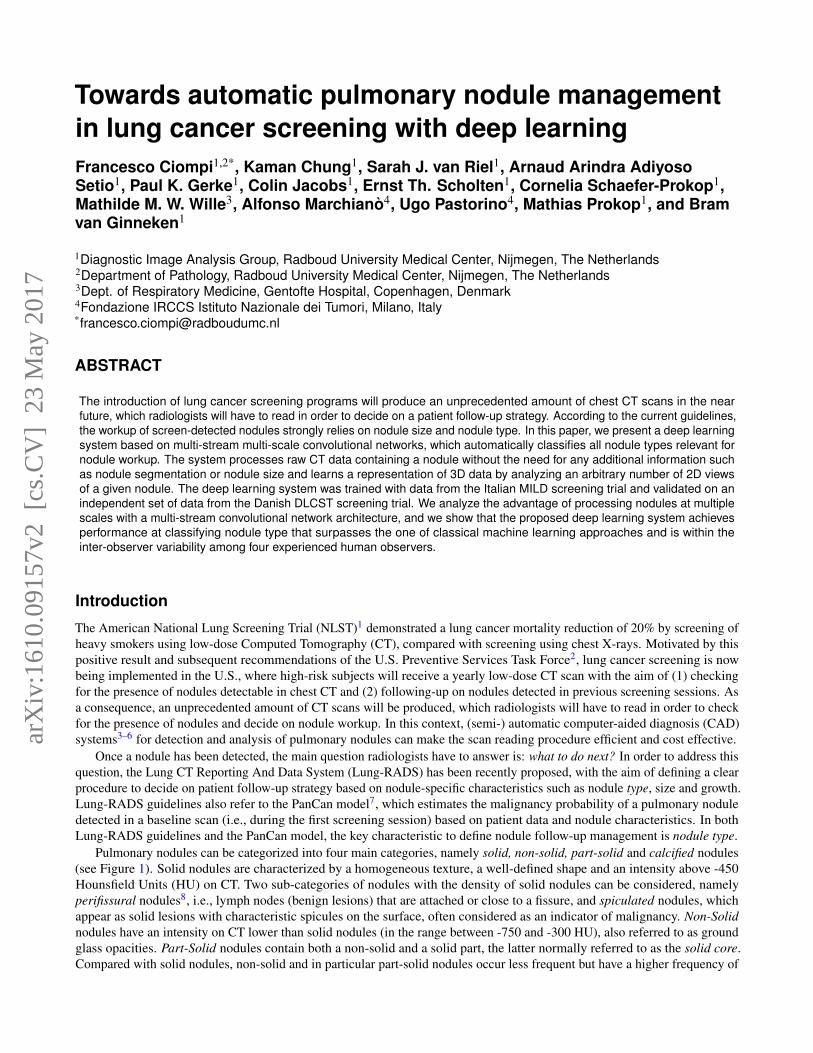
Pulmonary nodules can be categorized into four main categories, namely solid, non-solid, part-solid and calcified nodules(see Figure 1). Solid nodules are characterized by a homogeneous texture, a well-defined shape and an intensity above -450Hounsfield Units (HU) on CT. Two sub-categories of nodules with the density of solid nodules can be considered, namelyperifissural nodules8, i.e., lymph nodes (benign lesions) that are attached or close to a fissure, and spiculated nodules, whichappear as solid lesions with characteristic spicules on the surface, often considered as an indicator of malignancy. Non-Solidnodules have an intensity on CT lower than solid nodules (in the range between -750 and -300 HU), also referred to as groundglass opacities. Part-Solid nodules contain both a non-solid and a solid part, the latter normally referred to as the solid core.Compared with solid nodules, non-solid and in particular part-solid nodules occur less frequent but have a higher frequency of

arX

iv:1

610.

0915

7v2

[cs

.CV

] 2

3 M

ay 2

017

axial coronal sagittal

patch size = 10 mm

axial coronal sagittal axial coronal sagittal

patch size = 20 mm patch size = 40 mm

calcified

perifissural

solid

non-solid

part-solid

spiculated

Figure 1. Examples of triplets of patches for different nodule types in axial, coronal and sagittal views. Each triplet isdepicted using three different patch sizes, namely 10 mm, 20 mm and 40 mm.

being malignant lesions9. Finally, calcified nodules are characterized by a high intensity and a well-defined rounded shape onCT. Completely calcified nodules represent benign lesions.

In Lung-RADS, the workup for pulmonary nodules is mainly defined by nodule type and nodule size. However, presenceof imaging findings that increase the suspicion of lung cancer, such as spiculation, can modify the workup. In the PanCanmodel, spiculation is a parameter that together with nodule type, nodule size and patient data contribute to the estimation ofthe malignancy probability of a nodule. Furthermore, completely calcified and perifissural nodules are given a malignancyprobability equal to zero. In a scenario in which CAD systems are used to automate the lung cancer screening workflowfrom nodule detection to automatic report with decision on nodule workup, it is necessary to solve the problem of automaticclassification of nodule type. In this context, the classes that have to be considered are: (i) solid, (ii) non-solid, (iii) part-solid,(iv) calcified, (v) perifissural and (vi) spiculated nodules.

Although the general characteristics of nodule types can be easily defined, recent studies10, 11 have shown that there is asubstantial inter- and intra-observer variability among radiologists at classifying nodule type. In this context, researchers haveaddressed the problem of automatic classification of nodule type in CT scans by (1) designing a problem-specific descriptor oflung nodule and (2) training a classification model to automatically predict nodule type. In11, nodules were classified as solid,non-solid and part-solid. A nodule descriptor was designed based on information on volume, mass and intensity of the nodule,and a kNN classifier was applied, but the used features strongly rely on the result of a nodule segmentation algorithm, whoseoptimal settings also depend on nodule type. The authors propose to solve this problem by first running the algorithm multipletimes using different segmentation settings in order to extract features and then classify nodule type. In practice, this strategyhampers the applicability of such a system to an optimized scan reading scenario. In12, the SIFT descriptor was used to classifynodules as juxta, well circumscribed, pleural-tail and vascularized, and a feature matching strategy was used for classificationpurposes. Despite the good performance reported, the considered categories are not relevant for nodule management accordingto current guidelines. A descriptor specifically tailored for lung nodule analysis was introduced in13, which was used to assesspresence of spiculation in detected solid nodules14 and to classify nodules as perifissural15. Although this approach could beextended to other nodule types, it strongly relies on the estimation of nodule size in order to define the proper scale to analyzedata.

Scale is an important factor to consider in automatic nodule type classification. As an example, discriminating a pure solidnodule from a perifissural nodule involves the detection of the fissure, which on a 2D view of the nodule can be differentiatedfrom a vessel only if a sufficiently large region surrounding the nodule is considered (see Figure 1). On the other hand,discriminating non-solid from part-solid nodules strongly relies on the presence of a solid core, which can consist of a tiny part

2/12

MILD (943 patients) DLCST (468 patients)

Training nodules N Training samples Validation nodules Test nodules testALL / testOBS

Solid 694 8 88,832 232 382 / 27Calcified 233 22 82,016 78 58 / 27Part-solid 63 80 80,640 21 37 / 27Non-solid 152 33 80,256 50 87 / 27

Perifissural 181 28 81,088 62 48 / 27Spiculated 29 167 77,488 10 27 / 27

Total 1,352 – 490,320 453 639 / 162

Table 1. Detailed number of nodules and samples in the training, validation and test sets. The MILD dataset is used fortraining and validation purposes, the DLCST dataset is used for testing purposes. In the test set, the number of nodules perclass randomly selected to design the observer study is reported. The number of class-specific planes per nodule used to extracttraining data (N, see also Figure 4) is indicated for each nodule type. The number of used patients from MILD and DLCST arealso indicated.

of the lesion that can only be clearly detected on a small scale.In recent years, the advent of deep learning16, 17 has emerged as a powerful alternative to designing ad-hoc descriptors

for pattern recognition applications by using deep neural networks, which can learn a representation of data from the rawdata itself. The most used incarnation of deep neural networks are convolutional networks16, 18, 19, a supervised learningalgorithm particularly suited to solve problems of classification of natural images19–21, which has recently been applied to someapplications in chest CT analysis6, 15, 22–24.

In this paper, we address the problem of automatic nodule classification by introducing three main contributions. Forthe first time, we propose a single system that classifies all nodule types relevant for patient management in lung cancerscreening according to the Lung-RADS assessment categories and the PanCan malignancy probability model, namely solid,non-solid, part-solid, calcified, perifissural and spiculated nodules. Differently from what has been done in previous work, wedesign a classification framework based on Convolutional Networks (ConvNets)17–19. In particular, we propose a multi-streammulti-scale architecture in which ConvNets simultaneously process multiple triplets of 2D views of a nodule at multiple scalesand compute the probability for the nodule to belong to each one of the six considered nodule types. The proposed approachdoes not require nodule segmentation or the estimation of nodule size. Inspired by recent work6, 15, we formulate the analysis ofa nodule as a combination of 2D patches. Relying on the experimental results of Setio et al.6, which showed that performanceincrease by increasing the number of analyzed patches, we go beyond a limited number of patches by introducing a novelapproach to extract an arbitrary number of 2D views from a nodule. We trained the deep learning system using data from943 patients and 1,352 nodules from the Multicentric Italian Lung Detection (MILD) trial25 and we validated the trainedsystem using independent data from 468 patients and 639 nodules from the Danish Lung Cancer Screening Trial (DLCST)26.Furthermore, in order to compare the performance of our deep learning architecture versus classical approaches of patchclassification, we trained a linear support vector machines classifier to classify both features based on the raw intensity ofnodules and features learned from raw data via an unsupervised learning approach. Finally, in order to compare the performanceof our method versus human performance, we designed an observer study in which four observers, including experiencedradiologists, classified a subset of 162 nodules extracted from the test set. We show that the proposed system achievesperformance that surpasses classical patch classification approaches and is comparable with the inter-observer variability amonghuman observers.

Results

Training dataWe trained the deep learning system using data from the Multicentric Italian Lung Detection (MILD) trial25. For this purpose,we considered all baseline CT scans from the MILD trial. The study was approved by the Institutional review board ofFondazione IRCCS Istituto Nazionale Tumori di Milano, and the written informed consent was waived for the retrospectiveexamination of the analyzed data. For all patients, non contrast-enhanced low-dose CT scans were acquired using a 16-detectorrow CT system, with section collimation 16 × 0.75 mm. Images were reconstructed using a sharp kernel (Siemens B50 kernel,Siemens Medical Solutions) with a slice thickness of 1.0 mm. Nodules were detected and annotated based on the followingprocedure. All CT scans were first read by a workstation (CIRRUS Lung Screening, Diagnostic Image Analysis Group,Radboudumc, Nijmegen, Netherlands) with automatic nodule detection (CAD) tools integrated. Two medical students, trainedby a radiology research in detecting pulmonary nodules, either accepted or rejected CAD marks and labeled nodules as one ofthe considered nodule types. Accepted nodules were segmented using the algorithm presented in27, which is implemented

3/12

Observers Computer

O1 O2 O3 O4 1 scale 2 scales 3 scales

O1 – 0.59 (0.51–0.68) 0.65 (0.57–0.74) 0.68 (0.60–0.76) 0.63 (0.54–0.72) 0.64 (0.55–0.73) 0.65 (0.57–0.74)O2 0.59 (0.51–0.68) – 0.71 (0.63–0.79) 0.66 (0.58–0.75) 0.55 (0.45–0.64) 0.54 (0.45–0.64) 0.58 (0.49–0.67)O3 0.65 (0.57–0.74) 0.71 (0.63–0.79) – 0.75 (0.67–0.82) 0.56 (0.47–0.65) 0.57 (0.48–0.66) 0.61 (0.52–0.70)O4 0.68 (0.60–0.76) 0.66 (0.58–0.75) 0.75 (0.67–0.82) – 0.62 (0.53–0.70) 0.64 (0.55–0.73) 0.67 (0.59–0.75)

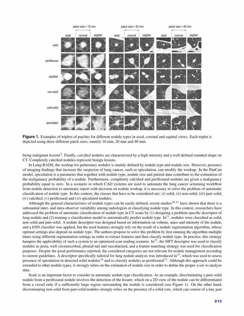
Table 2. Cohen κ statistics with 95% confidence intervals for agreement between computer and observers. Oi indicates thei-th observer. Results for automatic classification using deep learning systems with different numbers of scales are reported.

in CIRRUS Lung Screening. The students manually adjusted parameters to obtain the best possible nodule segmentation,which allowed to compute the equivalent diameter of the lesion. Nodules with label disagreement were reviewed by a thoracicradiologist (ES) with more than 20 years of experience in reading chest CT scans. Nodules with label agreement were furtherreviewed by two radiology researchers (SvR, KC) independently. From the set of annotated nodules, we removed all caseswith a diameter smaller than 4 mm, which is considered as an irrelevant finding in lung cancer screening1. The final set ofdata consisted of 1,805 nodules from 943 subjects (see Table 1), which were split into two non-overlapping sets: a training set(1,352 nodules), used to train the deep learning system and a validation set (453 nodules), used to monitor the performance ofthe system during training.

In the development of the proposed deep learning system, we defined a nodule data sample as a set of triplets of patches(axial, coronal and sagittal view), where each triplet was used to feed three streams of convolutional network (details ondata preprocessing, system design and training are detailed in the Methods section). For training purposes, several differentsamples were extracted from the same nodule by rotating triplets around the center of mass and by using techniques of dataaugmentation at patch level. In this way, ≈ 0.5M training samples were extracted and used to train the deep learning system. Inour experiments, we investigated the performance of the system when data at different scales were considered. For this purpose,we extracted nodule data with patches of size 10 mm, 20 mm and 40 mm, which represent 3 different scales. We built andtrained three network architectures where one scale (40 mm), two scales (20 mm, 40 mm) and three scales (10 mm, 20 mm, 40mm) were processed, and compared the performance of the three networks with both classical patch classification approachesbased on machine learning and human performance.

Test dataThe performance of the trained deep learning system was assessed on data from the Danish Lung Cancer Screening Trial(DLCST)26. In particular, we used the subset of data used in a study recently published by the DLCST research group28, wherethe authors also describe the procedure used to annotate nodule types. The DLCST was approved by the ethics committe ofCopenhagen County and fully funded by the Danish Ministry of Interior and Health. Approval of data management in the trialwas obtained from the Danish Data Protection Agency. The trial is registered with ClinicalTrials.gov (NCT00496977). Allparticipants provided written informed consent. Non contrast-enhanced low-dose CT scans were acquired using a multi-slice CTsystem (16-row Philips Mx 8000, Philips Medical Systems) with section collimation 16 × 0.75 mm. Images were reconstructedusing a sharp kernel (kernel D) with a slice thickness of 1.0 mm. From the initial data set, we removed nodules with a diametersmaller than 4 mm, as done for data from the MILD trial, and discarded scans with incomplete or corrupted data (e.g., missingslices). Finally, we obtained a set testALL of 639 nodules from 468 subjects (see Table 1), which we used for testing purposes.

Observer studyIn order to compare the deep learning system with human performance, we selected a subset of nodules from the set testALL andasked three observers to label nodule type. For this purpose, we built a dataset by including all spiculated nodules in testALL (27nodules) and the same number of nodules randomly selected from the other classes. Therefore, a dataset testOBS of 162 noduleswas built for the observer study. Two chest radiologists (ES, CSP) with more than 20 years of experience reading chest CT anda radiology researcher (KC) were involved in the observer study. Readers independently labeled nodule types. Nodules wereshown at locations indicated by annotations provided by the DLCST trial, and readers had the possibility to either label thenodule as belonging to one of the six considered categories, or label it as not a nodule. For evaluation purposes, we consideredannotations made by the three observers involved in this study as well as annotations coming from the DLCST trial, which weconsidered as an additional observer. In the rest of the paper we will refer to annotations coming from these four differentsources as observers O1, O2, O3 and O4 (where O4 indicates the DLCST annotations).

EvaluationAfter training, all nodules in testALL were classified using the trained deep learning system. In order to compute the computer-observer agreement, we compared the results from the computer with the nodule type given by each observer independently in

4/12

solid

calc

ified

part-

solid

non-

solid

perif

issu

ral

spic

ulat

ed

probability = 0 probability = 1

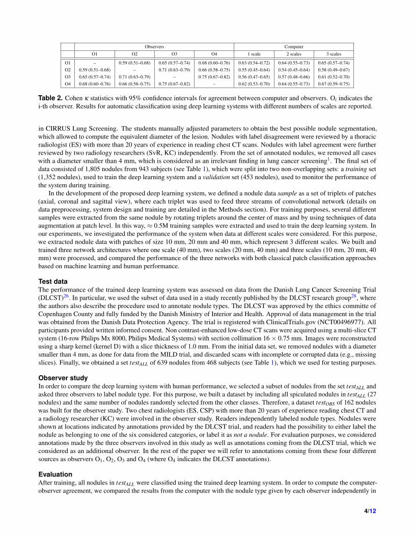
Figure 2. Examples of classified nodules from the test set (DLCST). Each row depicts nodules from one class as labeled inthe DLCST trial, and nodules are sorted from left to right based on the probability given by the (3-scale) deep learning system.Examples with low probability (on the left) are a-typical cases of each nodule type, while a high probability (on the right) isgiven to typical examples of each nodule type.

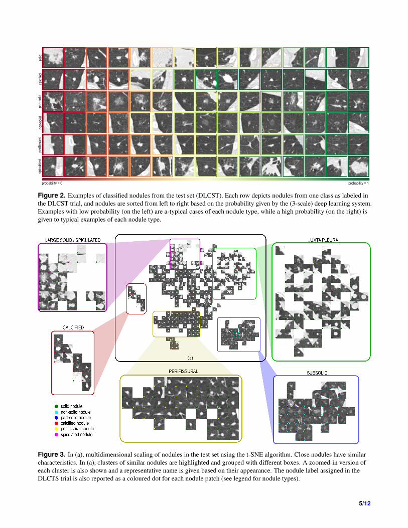
Figure 3. In (a), multidimensional scaling of nodules in the test set using the t-SNE algorithm. Close nodules have similarcharacteristics. In (a), clusters of similar nodules are highlighted and grouped with different boxes. A zoomed-in version ofeach cluster is also shown and a representative name is given based on their appearance. The nodule label assigned in theDLCTS trial is also reported as a coloured dot for each nodule patch (see legend for nodule types).

5/12

Accuracy FSolid FCalci f ied FPart−solid FNon−solid FPeri f issural FSpiculated FNot−a−nodule

O1 vs. Computer (3 scales) 71.5% 60.8% 88.4% 66.7% 86.3% 62.2% 71.4% –O2 vs. Computer (3 scales) 66.2% 62.6% 82.4% 47.8% 72.7% 80.0% 56.4% –O3 vs. Computer (3 scales) 67.7% 56.8% 85.1% 59.1% 78.3% 75.6% 60.9% –O4 vs. Computer (3 scales) 72.8% 64.2% 88.9% 71.7% 80.0% 77.3% 62.7% –

Average 69.6% 61.1% 86.2% 61.3% 79.3% 73.8% 62.9% –

O1 vs. O2 66.0% 52.7% 84.0% 51.3% 79.2% 63.6% 83.3% 50.0%O1 vs. O3 71.0% 55.0% 87.0% 66.7% 80.0% 81.5% 74.4% 40.0%O1 vs. O4 72.8% 64.8% 90.9% 66.7% 71.7% 75.5% 89.4% 0.0%O2 vs. O3 76.5% 74.7% 88.9% 61.5% 81.0% 77.3% 75.7% 66.7%O2 vs. O4 72.2% 64.4% 88.5% 70.8% 71.1% 79.1% 73.2% 0.0%O3 vs. O4 79.0% 68.4% 95.8% 71.1% 80.9% 90.6% 79.2% 0.0%

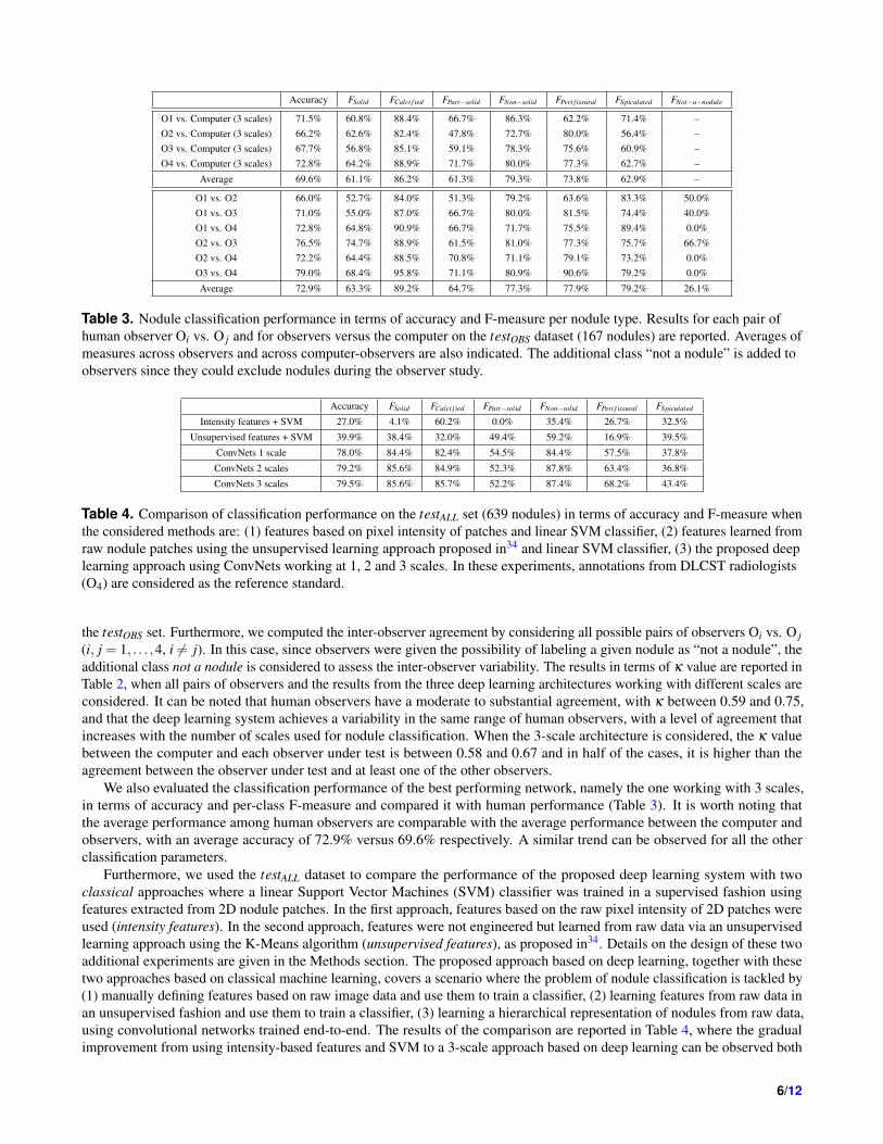
Average 72.9% 63.3% 89.2% 64.7% 77.3% 77.9% 79.2% 26.1%

Table 3. Nodule classification performance in terms of accuracy and F-measure per nodule type. Results for each pair ofhuman observer Oi vs. O j and for observers versus the computer on the testOBS dataset (167 nodules) are reported. Averages ofmeasures across observers and across computer-observers are also indicated. The additional class “not a nodule” is added toobservers since they could exclude nodules during the observer study.

Accuracy FSolid FCalci f ied FPart−solid FNon−solid FPeri f issural FSpiculated

Intensity features + SVM 27.0% 4.1% 60.2% 0.0% 35.4% 26.7% 32.5%

Unsupervised features + SVM 39.9% 38.4% 32.0% 49.4% 59.2% 16.9% 39.5%

ConvNets 1 scale 78.0% 84.4% 82.4% 54.5% 84.4% 57.5% 37.8%

ConvNets 2 scales 79.2% 85.6% 84.9% 52.3% 87.8% 63.4% 36.8%

ConvNets 3 scales 79.5% 85.6% 85.7% 52.2% 87.4% 68.2% 43.4%

Table 4. Comparison of classification performance on the testALL set (639 nodules) in terms of accuracy and F-measure whenthe considered methods are: (1) features based on pixel intensity of patches and linear SVM classifier, (2) features learned fromraw nodule patches using the unsupervised learning approach proposed in34 and linear SVM classifier, (3) the proposed deeplearning approach using ConvNets working at 1, 2 and 3 scales. In these experiments, annotations from DLCST radiologists(O4) are considered as the reference standard.

the testOBS set. Furthermore, we computed the inter-observer agreement by considering all possible pairs of observers Oi vs. O j(i, j = 1, . . . ,4, i 6= j). In this case, since observers were given the possibility of labeling a given nodule as “not a nodule”, theadditional class not a nodule is considered to assess the inter-observer variability. The results in terms of κ value are reported inTable 2, when all pairs of observers and the results from the three deep learning architectures working with different scales areconsidered. It can be noted that human observers have a moderate to substantial agreement, with κ between 0.59 and 0.75,and that the deep learning system achieves a variability in the same range of human observers, with a level of agreement thatincreases with the number of scales used for nodule classification. When the 3-scale architecture is considered, the κ valuebetween the computer and each observer under test is between 0.58 and 0.67 and in half of the cases, it is higher than theagreement between the observer under test and at least one of the other observers.

We also evaluated the classification performance of the best performing network, namely the one working with 3 scales,in terms of accuracy and per-class F-measure and compared it with human performance (Table 3). It is worth noting thatthe average performance among human observers are comparable with the average performance between the computer andobservers, with an average accuracy of 72.9% versus 69.6% respectively. A similar trend can be observed for all the otherclassification parameters.

Furthermore, we used the testALL dataset to compare the performance of the proposed deep learning system with twoclassical approaches where a linear Support Vector Machines (SVM) classifier was trained in a supervised fashion usingfeatures extracted from 2D nodule patches. In the first approach, features based on the raw pixel intensity of 2D patches wereused (intensity features). In the second approach, features were not engineered but learned from raw data via an unsupervisedlearning approach using the K-Means algorithm (unsupervised features), as proposed in34. Details on the design of these twoadditional experiments are given in the Methods section. The proposed approach based on deep learning, together with thesetwo approaches based on classical machine learning, covers a scenario where the problem of nodule classification is tackled by(1) manually defining features based on raw image data and use them to train a classifier, (2) learning features from raw data inan unsupervised fashion and use them to train a classifier, (3) learning a hierarchical representation of nodules from raw data,using convolutional networks trained end-to-end. The results of the comparison are reported in Table 4, where the gradualimprovement from using intensity-based features and SVM to a 3-scale approach based on deep learning can be observed both

6/12

Solid Calcified Part-solid Non-solid Perifissural Spiculated

Precision 89.2 88.9 43.6 87.4 78.4 32.7

Recall 82.2 82.8 64.9 87.4 60.4 64.3

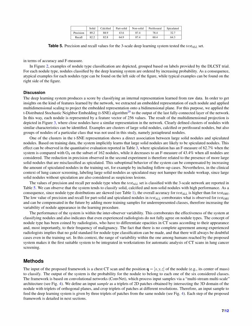
Table 5. Precision and recall values for the 3-scale deep learning system tested the testALL set.

in terms of accuracy and F-measure.In Figure 2, examples of nodule type classification are depicted, grouped based on labels provided by the DLCST trial.

For each nodule type, nodules classified by the deep learning system are ordered by increasing probability. As a consequence,atypical examples for each nodules type can be found on the left side of the figure, while typical examples can be found on theright side of the figure.

DiscussionThe deep learning system produces a score by classifying an internal representation learned from raw data. In order to getinsights on the kind of features learned by the network, we extracted an embedded representation of each nodule and appliedmultidimensional scaling to project the embedded representation onto a bidimensional plane. For this purpose, we applied thet-Distributed Stochastic Neighbor Embedding (t-SNE) algorithm29 to the output of the last fully-connected layer of the network.In this way, each nodule is represented by a feature vector of 256 values. The result of the multidimensional projection isdepicted in Figure 3, where close nodules have a similar representation in the network. Clearly defined clusters of nodules withsimilar characteristics can be identified. Examples are clusters of large solid nodules, calcified or perifissural nodules, but alsogroups of nodules of a particular class that was not used in this study, namely juxtapleural nodules.

One of the clusters in the t-SNE representation shows a direct association between large solid nodules and spiculatednodules. Based on training data, the system implicitly learns that large solid nodules are likely to be spiculated nodules. Thiseffect can be observed in the quantitative evaluation reported in Table 3, where spiculation has an F-measure of 62.7% when thesystem is compared with O4 on the subset of 162 nodules, while it decreases to an F-measure of 43.4% when all nodules areconsidered. The reduction in precision observed in the second experiment is therefore related to the presence of more largesolid nodules that are misclassified as spiculated. This suboptimal behavior of the system can be compensated by increasingthe amount of spiculated nodules in the training set, for example by including follow-up cases. Nevertheless, in the clinicalcontext of lung cancer screening, labeling large solid nodules as spiculated may not hamper the nodule workup, since largesolid nodules without spiculation are also considered as suspicious lesions.

The values of precision and recall per nodule type when the testALL set is classified with the 3-scale network are reported inTable 5. We can observe that the system tends to classify solid, calcified and non-solid nodules with high performance. As aconsequence, since nodule type distributions are skewed (see Table 1), the overall accuracy for testALL is higher than for testOBS.The low value of precision and recall for part-solid and spiculated nodules in testALL corroborates what is observed for testOBSand can be compensated in the future by adding more training samples for underrepresented classes, therefore increasing thevariability of nodule appearance in the learning procedure.

The performance of the system is within the inter-observer variability. This corroborates the effectiveness of the system atclassifying nodules and also indicates that even experienced radiologists do not fully agree on nodule types. The concept ofnodule type has been coined by radiologists, who have to differentiate opacities in CT scans according to their appearanceand, most importantly, to their frequency of malignancy. The fact that there is no complete agreement among experiencedradiologists implies that no gold standard for nodule type classification can be made, and that there will always be doubtfulcases even in the training set. In this context, the range of variability within the one among humans reached by the proposedsystem makes it the first suitable system to be integrated in workstations for automatic analysis of CT scans in lung cancerscreening.

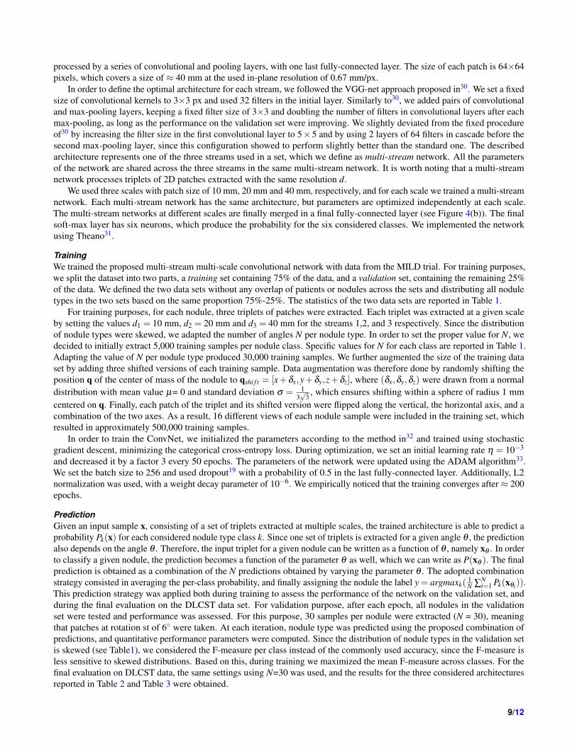
MethodsThe input of the proposed framework is a chest CT scan and the position q = [x,y,z] of the nodule (e.g., its center of mass)to classify. The output of the system is the probability for the nodule to belong to each one of the six considered classes.The framework is based on convolutional networks (ConvNet), which process input samples via a “multi-stream multi-scale”architecture (see Fig. 4). We define an input sample as a triplets of 2D patches obtained by intersecting the 3D domain of thenodule with triplets of orthogonal planes, and crop triplets of patches at different resolutions. Therefore, an input sample tofeed the deep learning system is given by three triplets of patches from the same nodule (see Fig. 4). Each step of the proposedframework is detailed in next sections.

7/12

32@5x5

pooling2

64@3x3

pooling2

128@3x3

pooling2

256@3x3

pooling2

32@5x5

pooling2

64@3x3

pooling2

128@3x3

pooling2

256@3x3

pooling2

32@5x5

pooling2

64@3x3

pooling2

128@3x3

pooling2

256@3x3

pooling2

FC-128 FC-128 FC-128

32@5x5

pooling2

64@3x3

pooling2

128@3x3

pooling2

256@3x3

pooling2

32@5x5

pooling2

64@3x3

pooling2

128@3x3

pooling2

256@3x3

pooling2

32@5x5

pooling2

64@3x3

pooling2

128@3x3

pooling2

256@3x3

pooling2

FC-128 FC-128 FC-128

32@5x5

pooling2

64@3x3

pooling2

128@3x3

pooling2

256@3x3

pooling2

32@5x5

pooling2

64@3x3

pooling2

128@3x3

pooling2

256@3x3

pooling2

32@5x5

pooling2

64@3x3

pooling2

128@3x3

pooling2

256@3x3

pooling2

FC-128 FC-128 FC-128

FC-256

softmax-6

scale 10 mm scale 20 mm scale 40 mm

convolutional layer (n_filters@filter_size x filter_size)

pooling layer (poolingwindow_size)

fully-connected layer (FC-n_units)

soft-max layer (softmax-n_units)

P

(a) (b)

axialcoronalsagittal

q=[x,y,z]d = 10mm (64 px) d = 20mm (64 px) d = 40mm (64 px)

64@3x3 64@3x3 64@3x3 64@3x3 64@3x3 64@3x3 64@3x3 64@3x3 64@3x3

Figure 4. (a) Examples of triplets of nodules extracted by varying the parameter N. (b) Examples of pyramidal triplets ofpatches used to feed the proposed deep learning systems. The system consists of three groups of three streams, one for eachconsidered scale (namely 10 mm, 20 mm and 40 mm for patch size). Convolutional layers, max-pooling layers, fully-connectedlayers and one soft-max layer are the building blocks of the proposed network. The last fully-connected layer with 256 neuronsserves as a combiner of the three sets of three streams, and a 6-value probability vector is generated as output.

Generation of triplets of 2D patchesLet us define a triplet of orthogonal planes Tn = Ψn,Ωh,Φn passing through the point q and an angle θn = (n−1)π

2N(n = 1, . . . ,N), which defines the rotation of each plane of Tn with respect to the axes x,y,z. In this way, T1 is the triplet ofplanes that define the default axial, coronal and sagittal views of a CT scan, and any other triplet Tn is obtained by sequentiallyrotating the triplet with respect to the x, the y and the z axis by an angle θn. Rotating all the planes by the same angle guaranteesthat orthogonal planes are always obtained. Examples of triplets for several values of N are depicted in Figure 4(a), where theaxial, coronal and sagittal planes are represented in different colors.

The intersection of a triplet of planes and a CT scan generates 2D views of the nodule of interest. From each intersection, wegenerate triplets of 2D patches by cropping a square area of size d centered on q. Increasing the value of N allows to increasethe number of extracted patches per nodule, which also increases the coverage of the volume of a nodule in 3D. Furthermore,adapting the value of N per nodule type has the advantage of (1) balancing classes distribution in the presence of skeweddistribution of classes by using a larger value of N for underrepresented classes, and (2) using it as a kind of data augmentation,in which many different views of the same object are extracted.

The parameter d defines the scale at which patches are considered. Using multiple values of d allows to crop triplets ofpatches with information that range from local content to more global context of nodule appearance. In order to train theproposed deep learning system, we extracted triplets of patches at three different scales, namely d = 10,20,40 mm and fedthree streams of the network with three triplets at the same time. This allows the network to focus both on the local appearanceof a nodule (10 mm), where small structures like the solid core can be analyzed, and on more global context (40 mm), in whichstructures like the fissure can be recognized. Before feeding the network, each patch was rescaled to a fixed size of 64×64pixels using bicubic interpolation and the pixel intensity IHU ∈ [−1200,400] HU was rescaled to Inorm ∈ [0,1] by applying thetransformation Inorm = IHU+1200

1600 .

Deep learning networkNetwork designThe architecture of the used deep learning system is depicted in Figure 4(b). The system consists of nine streams of ConvNets,grouped into three sets of three streams. Each set of streams is fed with a triplet of orthogonal patches extracted at the samescale. Different sets of streams process triplets of orthogonal patches with exactly the same orientation in the CT scan, but atdifferent scales. Each stream of the set is fed with one patch from a triplet of orthogonal patches. The 2D input patch is then

8/12

processed by a series of convolutional and pooling layers, with one last fully-connected layer. The size of each patch is 64×64pixels, which covers a size of ≈ 40 mm at the used in-plane resolution of 0.67 mm/px.

In order to define the optimal architecture for each stream, we followed the VGG-net approach proposed in30. We set a fixedsize of convolutional kernels to 3×3 px and used 32 filters in the initial layer. Similarly to30, we added pairs of convolutionaland max-pooling layers, keeping a fixed filter size of 3×3 and doubling the number of filters in convolutional layers after eachmax-pooling, as long as the performance on the validation set were improving. We slightly deviated from the fixed procedureof30 by increasing the filter size in the first convolutional layer to 5×5 and by using 2 layers of 64 filters in cascade before thesecond max-pooling layer, since this configuration showed to perform slightly better than the standard one. The describedarchitecture represents one of the three streams used in a set, which we define as multi-stream network. All the parametersof the network are shared across the three streams in the same multi-stream network. It is worth noting that a multi-streamnetwork processes triplets of 2D patches extracted with the same resolution d.

We used three scales with patch size of 10 mm, 20 mm and 40 mm, respectively, and for each scale we trained a multi-streamnetwork. Each multi-stream network has the same architecture, but parameters are optimized independently at each scale.The multi-stream networks at different scales are finally merged in a final fully-connected layer (see Figure 4(b)). The finalsoft-max layer has six neurons, which produce the probability for the six considered classes. We implemented the networkusing Theano31.

TrainingWe trained the proposed multi-stream multi-scale convolutional network with data from the MILD trial. For training purposes,we split the dataset into two parts, a training set containing 75% of the data, and a validation set, containing the remaining 25%of the data. We defined the two data sets without any overlap of patients or nodules across the sets and distributing all noduletypes in the two sets based on the same proportion 75%-25%. The statistics of the two data sets are reported in Table 1.

For training purposes, for each nodule, three triplets of patches were extracted. Each triplet was extracted at a given scaleby setting the values d1 = 10 mm, d2 = 20 mm and d3 = 40 mm for the streams 1,2, and 3 respectively. Since the distributionof nodule types were skewed, we adapted the number of angles N per nodule type. In order to set the proper value for N, wedecided to initially extract 5,000 training samples per nodule class. Specific values for N for each class are reported in Table 1.Adapting the value of N per nodule type produced 30,000 training samples. We further augmented the size of the training dataset by adding three shifted versions of each training sample. Data augmentation was therefore done by randomly shifting theposition q of the center of mass of the nodule to qshi f t = [x+δx,y+δy,z+δz], where (δx,δy,δz) were drawn from a normaldistribution with mean value µ= 0 and standard deviation σ = 1

3√

3, which ensures shifting within a sphere of radius 1 mm

centered on q. Finally, each patch of the triplet and its shifted version were flipped along the vertical, the horizontal axis, and acombination of the two axes. As a result, 16 different views of each nodule sample were included in the training set, whichresulted in approximately 500,000 training samples.

In order to train the ConvNet, we initialized the parameters according to the method in32 and trained using stochasticgradient descent, minimizing the categorical cross-entropy loss. During optimization, we set an initial learning rate η = 10−3

and decreased it by a factor 3 every 50 epochs. The parameters of the network were updated using the ADAM algorithm33.We set the batch size to 256 and used dropout19 with a probability of 0.5 in the last fully-connected layer. Additionally, L2normalization was used, with a weight decay parameter of 10−6. We empirically noticed that the training converges after ≈ 200epochs.

PredictionGiven an input sample x, consisting of a set of triplets extracted at multiple scales, the trained architecture is able to predict aprobability Pk(x) for each considered nodule type class k. Since one set of triplets is extracted for a given angle θ , the predictionalso depends on the angle θ . Therefore, the input triplet for a given nodule can be written as a function of θ , namely xθ . In orderto classify a given nodule, the prediction becomes a function of the parameter θ as well, which we can write as P(xθ ). The finalprediction is obtained as a combination of the N predictions obtained by varying the parameter θ . The adopted combinationstrategy consisted in averaging the per-class probability, and finally assigning the nodule the label y = argmaxk(

1N ∑

Ni=1 Pk(xθi)).

This prediction strategy was applied both during training to assess the performance of the network on the validation set, andduring the final evaluation on the DLCST data set. For validation purpose, after each epoch, all nodules in the validationset were tested and performance was assessed. For this purpose, 30 samples per nodule were extracted (N = 30), meaningthat patches at rotation st of 6 were taken. At each iteration, nodule type was predicted using the proposed combination ofpredictions, and quantitative performance parameters were computed. Since the distribution of nodule types in the validation setis skewed (see Table1), we considered the F-measure per class instead of the commonly used accuracy, since the F-measure isless sensitive to skewed distributions. Based on this, during training we maximized the mean F-measure across classes. For thefinal evaluation on DLCST data, the same settings using N=30 was used, and the results for the three considered architecturesreported in Table 2 and Table 3 were obtained.

9/12

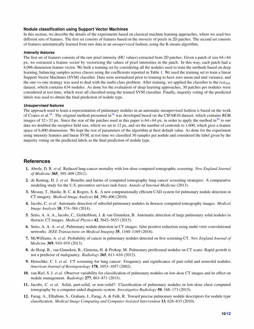
Nodule classification using Support Vector MachinesIn this section, we describe the details of the experiments based on classical machine learning approaches, where we used twodifferent sets of features. The first set consists of features based on the intensity of pixels in 2D patches. The second set consistsof features automatically learned from raw data in an unsupervised fashion, using the K-means algorithm.

Intensity featuresThe first set of features consists of the raw pixel intensity (HU values) extracted from 2D patches. Given a patch of size 64×64px, we extracted a feature vector by vectorizing the values of pixel intensities in the patch. In this way, each patch had a4,096-dimension feature vector. We built a training set by considering all the nodules used to train the methods based on deeplearning, balancing samples across classes using the coefficients reported in Table 1. We used the training set to train a linearSupport Vector Machines (SVM) classifier. Data were normalized prior to training to have zero mean and unit variance, andthe one-vs-one strategy was used to deal with the multi-class problem. After training, we applied the classifier to the testALLdataset, which contains 634 nodules. As done for the evaluation of deep learning approaches, 30 patches per nodules wereconsidered at test time, which were all classified using the trained SVM classifier. Finally, majority voting of the predictedlabels was used to obtain the final prediction of nodule type.

Unsupervised featuresThe approach used to learn a representation of pulmonary nodules in an automatic unsupervised fashion is based on the workof Coates et al.34. The original method presented in34 was developed based on the CIFAR10 dataset, which contains RGBimages of 32×32 px. Since the size of the patches used in this paper is 64×64 px, in order to apply the method in34 to ourdata we doubled the receptive field size, which we set to 12 px, and set the number of centroids to 1,600, which gave a featurespace of 6,400 dimensions. We kept the rest of parameters of the algorithm at their default value. As done for the experimentusing intensity features and linear SVM, at test time we classified 30 samples per nodule and considered the label given by themajority voting on the predicted labels as the final prediction of nodule type.

References1. Aberle, D. R. et al. Reduced lung-cancer mortality with low-dose computed tomographic screening. New England Journal

of Medicine 365, 395–409 (2011).

2. de Koning, H. J. et al. Benefits and harms of computed tomography lung cancer screening strategies: A comparativemodeling study for the U.S. preventive services task force. Annals of Internal Medicine (2013).

3. Messay, T., Hardie, R. C. & Rogers, S. K. A new computationally efficient CAD system for pulmonary nodule detection inCT imagery. Medical Image Analysis 14, 390–406 (2010).

4. Jacobs, C. et al. Automatic detection of subsolid pulmonary nodules in thoracic computed tomography images. MedicalImage Analysis 18, 374–384 (2014).

5. Setio, A. A. A., Jacobs, C., Gelderblom, J. & van Ginneken, B. Automatic detection of large pulmonary solid nodules inthoracic CT images. Medical Physics 42, 5642–5653 (2015).

6. Setio, A. A. A. et al. Pulmonary nodule detection in CT images: false positive reduction using multi-view convolutionalnetworks. IEEE Transactions on Medical Imaging 35, 1160–1169 (2016).

7. McWilliams, A. et al. Probability of cancer in pulmonary nodules detected on first screening CT. New England Journal ofMedicine 369, 910–919 (2013).

8. de Hoop, B., van Ginneken, B., Gietema, H. & Prokop, M. Pulmonary perifissural nodules on CT scans: Rapid growth isnot a predictor of malignancy. Radiology 265, 611–616 (2012).

9. Henschke, C. I. et al. CT screening for lung cancer: Frequency and significance of part-solid and nonsolid nodules.American Journal of Roentgenology 178, 1053–1057 (2002).

10. van Riel, S. J. et al. Observer variability for classification of pulmonary nodules on low-dose CT images and its effect onnodule management. Radiology 277, 863–871 (2015).

11. Jacobs, C. et al. Solid, part-solid, or non-solid?: Classification of pulmonary nodules in low-dose chest computedtomography by a computer-aided diagnosis system. Investigative Radiology 50, 168–173 (2015).

12. Farag, A., Elhabian, S., Graham, J., Farag, A. & Falk, R. Toward precise pulmonary nodule descriptors for nodule typeclassification. Medical Image Computing and Computer-Assisted Intervention 13, 626–633 (2010).

10/12

13. Ciompi, F. et al. Bag of frequencies: a descriptor of pulmonary nodules in computed tomography images. IEEETransactions on Medical Imaging 34, 1–12 (2015).

14. Ciompi, F. et al. Automatic detection of spiculation of pulmonary nodules in computed tomography images. In MedicalImaging, vol. 9414 of Proceedings of the SPIE (2015).

15. Ciompi, F. et al. Automatic classification of pulmonary peri-fissural nodules in computed tomography using an ensembleof 2D views and a convolutional neural network out-of-the-box. Medical Image Analysis 26, 195–202 (2015).

16. LeCun, Y., Bengio, Y. & Hinton, G. Deep learning. Nature 521, 436–444 (2015).

17. Schmidhuber, J. Deep learning in neural networks: an overview. Neural Networks 61, 85–117 (2015).

18. Lecun, Y., Bottou, L., Bengio, Y. & Haffner, P. Gradient-based learning applied to document recognition. Proceedings ofthe IEEE 86, 2278–2324 (1998).

19. Krizhevsky, A., Sutskever, I. & Hinton, G. Imagenet classification with deep convolutional neural networks. In Advancesin Neural Information Processing Systems 25, 1097–1105 (2012).

20. Sermanet, P. et al. OverFeat: Integrated recognition, localization and detection using convolutional networks. InInternational Conference on Learning Representations (ICLR 2014) (2014). ArXiv: 1312.6229.

21. Szegedy, C. et al. Going deeper with convolutions. arXiv:14094842v1 (2014).

22. van Ginneken, B., Setio, A. A. A., Jacobs, C. & Ciompi, F. Off-the-shelf convolutional neural network features forpulmonary nodule detection in computed tomography scans. In IEEE International Symposium on Biomedical Imaging,286–289 (2015).

23. Sebastian Roberto Tarando, A. F., Catalin Fetita & Brillet, P.-Y. Increasing cad system efficacy for lung texture analysisusing a convolutional network. In Medical Imaging, Proceedings of the SPIE (2016).

24. Anthimopoulos, M., Christodoulidis, S., Ebner, L., Christe, A. & Mougiakakou, S. Lung pattern classification for interstitiallung diseases using a deep convolutional neural network 35, 1207–1216 (2016).

25. Pastorino, U. et al. Annual or biennial CT screening versus observation in heavy smokers: 5-year results of the MILD trial.European Journal of Cancer Prevention 21, 308–315 (2012).

26. Pedersen, J. H. et al. The Danish randomized lung cancer CT screening trial–overall design and results of the prevalenceround. Journal of Thoracic Oncology 4, 608–614 (2009).

27. Kuhnigk, J. M. et al. Morphological segmentation and partial volume analysis for volumetry of solid pulmonary lesions inthoracic CT scans. IEEE Transactions on Medical Imaging 25, 417–434 (2006).

28. Winkler Wille, M. M. et al. Predictive accuracy of the pancan lung cancer risk prediction model -external validation basedon CT from the danish lung cancer screening trial. European Radiology 25, 3093–3099 (2015).

29. van der Maaten, L. & Hinton, G. Visualizing data using t-SNE 2579–2605 (2008).

30. Simonyan, K. & Zisserman, A. Very deep convolutional networks for large-scale image recognition. arXiv:14091556(2014).

31. Bastien, F. et al. Theano: new features and speed improvements. Deep Learning and Unsupervised Feature Learning NIPS2012 Workshop (2012).

32. Glorot, X. & Bengio, Y. Understanding the difficulty of training deep feedforward neural networks. In Internationalconference on artificial intelligence and statistics, 249–256 (2010).

33. Kingma, D. & Ba, J. ADAM: A method for stochastic optimization. arXiv:14126980 (2015).

34. Coates, A., Lee, H. & Ng, A. Y. An analysis of single-layer networks in unsupervised feature learning. In AISTATS (2011).

AcknowledgementsThis project was funded by a research grant from the Netherlands Organization for Scientific Research, project number639.023.207. The MILD project was supported by grants from the Italian Association for Cancer Research (AIRC): IG researchgrant 11991 and the special program Innovative Tools for Cancer Risk Assessment and early Diagnosis, 5 1000, No.12162;Italian Ministry of Health (RF- 2010). The authors would like to thank NVIDIA Corporation for the donation of a GeForceGTX Titan X graphics card used in the experiments.

11/12

Author contributions statementF.C. conceived and conducted the experiments, analysed the results and wrote the manuscript. K.C. trained students forannotating training data, reviewed training set annotations and took part in the observer study. S.v.R. reviewed training setannotations. A.S. and P.G. assisted in the technical development of the deep learning system. C.J. assisted in data selection.E.T.S. reviewed training data annotations and took part in the observer study. C.S.P. took part in the observer study. M.W.provided data for the evaluation of the method. A.M. and U.P. provided data for the training of the method. M.P. and B.v.G.designed and directed the study. All authors reviewed the manuscript.

Additional informationCompeting financial interests. Colin Jacobs received a research grant from MeVis Medical Solutions AG, Bremen, Germany.Bram van Ginneken receives research support from MeVis Medical Solutions and is co-founder and stockholder of Thirona.

12/12