Flexible Rerouting of Public Transit Under Uncertainty. In 14th International
Science of Smart City Operations and Platforms Engineering (SCOPE’19),
April 15, 2019, Montreal, QC, Canada. ACM, New York, NY, USA, 6 pages.
https://doi.org/10.1145/3313237.3313302
1 INTRODUCTION
The transit network in Nashville and other similarly sized cities are
challenged with lack of cross-town options as well as low frequency
Permission to make digital or hard copies of all or part of this work for personal orclassroom use is granted without fee provided that copies are not made or distributedfor profit or commercial advantage and that copies bear this notice and the full citationon the first page. Copyrights for components of this work owned by others than ACMmust be honored. Abstracting with credit is permitted. To copy otherwise, or republish,to post on servers or to redistribute to lists, requires prior specific permission and/or afee. Request permissions from [email protected].
of public transit service. Transit routes are generally static in nature,
i.e., they operate along pre-determined routes and at a designed fre-
quency; this service is typically referred to as Fixed-Route Transit
(FRT) [14]. Such fixed-route systems work well when the people
using the transit services are closer to the transit routes; this is typ-
ically seen in densely-populated metropolitan cities [11]. Demand
Responsive Transit (DRT) [14] systems have become a popular
form of public transit in rural and low-demand areas; these transit
systems have flexible pick-up and drop-off locations depending on
the travel demand. In this paper, we are interested in a specific case
of medium-sized cities such as Nashville where addition of fixed
routes in the fixed-route transit is not economically possible and
demand responsive transit systems are inefficient as the demand
in Nashville is higher than the regions (rural areas) where DRT
systems are typically used.
The fixed-route strategy may not work in smaller cities where
the population are spread across a region. People living in locations
not served by the transit network resort to using other forms of
transportation such as personal vehicles or ride-sharing services.
The problem with private transport is that their efficiency to the
travel demand is low, i.e., they carry few people and this results in
traffic congestion due to increase in the number of private vehicles,
used to meet the travel demand [3].
To avoid such traffic congestion, available public transit needs to
be used efficiently, i.e., serve as many people as possible. Moreover,
the existing road networks may not be sustainable with the ever-
increasing travel demand through increased use of private vehicles,
as new roads cannot be built at the same rate of increase in travel
demand. Efficient and reliable use of public transit resources can
help streamline the traffic flow process. Furthermore, they are safer
compared to the use of automotive vehicles in terms of the number
of accidents per passenger mile [9] and also the use of public transit
services makes the people more healthy as it requires for them to
walk/bike to the nearest bus stop [5].
However, typically transit services, are routed through fixed pre-
determined travel stops and pre-determined schedule, while it is
known that the travel demand shows both spatial and temporal
variability, where the number of people using the transit services
appear with the time of day and the geographic locations. In our
previous work [16], we showed that a transit schedule that varies
with seasons is more efficient compared to a static schedule, how-
ever, as discussed in that paper even seasonal variations are not
optimal and we need a more flexible public transit system.
Flexible transportation systems (FTS) [12] can be considered as
a hybrid of FRT and DRT, and are increasingly becoming popular
in regions where DRT and FRT are inefficient. Several forms of FTS
exist varying from near-FRT to near-DRT systems such as Route De-
viation, Point Deviation, Demand Responsive Connector, Request
35
SCOPE’19, April 15, 2019, Montreal, QC, Canada Saideep Nannapaneni and Abhishek Dubey
Stops, Flexible Route Segments and Zone Routes [12]. Depending
on the region and the nature of travel demand, an appropriate FTS
is used. In this paper, we utilize the advantages of FTS, particu-
larly the Route Deviation service, to accommodate the spatial and
temporal variation of travel demand in medium-size cities such as
Nashville. Route Deviation refers to the FTS, where a bus deviates
from its fixed route, to accommodate any passenger or para-transit
requests to pick-up and drop-off at requested locations.
Challenges: Previous literature [10, 13, 14] have studied Route
Deviation-based FTS; however, the bus stops made in the deviated
routes are determined based on the passenger requests and the
local transit authority. Such human-involved decision-making re-
garding the route deviations and flex stops may not be feasible in
the presence of large number of passenger requests as the number
of possible route deviations increases rapidly. In this paper, we
propose an efficient and automated approach based on clustering
and discrete optimization to identify the flex stops and the best
route deviation to maximize the accessibility of the public transit.
Research Contributions: The overall contributions made in
this paper are: (1) Identification of flex bus stops through density-
based clustering, and (2) Computation of the best rerouting strategy
through a discrete optimization to serve as many people as possible
and thus reduce travel congestion, while still serving fixed route
stops identified as critical.
Paper Organization: Section 2 provides the necessary defini-
tions, discusses the issues that need to be addressed and illustrates
them using Route 7 operated by the Nashville Metropolitan Author-
ity (MTA). Section 3 provides the assumptions and discusses the
proposed solution methodology for rerouting public transit under
spatial and temporal variations of travel demand. Implementation
of the solution for Route 7 operated by Nashville MTA is detailed in
Section 4. Concluding remarks and future work follow in Section 5.
2 PRELIMINARIES
2.1 Definitions
Scheduled Route: A bus route between start and end points, with
pre-determined stops, as scheduled by a local transit authority.
Critical bus stops: Critical bus stops refer to the bus stops that
can not be ignored, i.e., buses have to halt at these bus stops. In this
paper, the following bus stops are treated as critical bus stops bus
stops: (1) Bus stops with historical high passenger demand, and (2)
Transfer points, i.e., bus junctions where people change buses to
reach their destinations.
Non-critical bus stops: As the name suggests, these bus stops
can be ignored by the buses when there is no potential boarding
or getting off activity at the bus stops. This activity will be derived
from mobile applications and on-call kiosks at the transit-stops [7].
Flex Route: Flex route refers to a deviated route from the origi-
nal scheduled route in order to be accessible to more people. Flex
route are beneficial as they help eliminate the traffic congestion
caused when the people on the flex route take cabs or ride sharing
services to reach nearby bus stops or their final destinations.
Flex Stops: Flex-stops are new dynamic stops on a flex route
where people can gather and board the bus. This is an on-demand
feature (but not real-time, see the assumptions below in Section
2.2) and works through deviations around the non-critical stops.
Trip: A trip is defined as a bus journey from the start point to
the end point of a scheduled route.
Trip segment: A trip segment is a portion of a trip, which con-
sists of fewer transit stops compared to the overall trip.
Trip Block: A trip block represents a sequence of trips between
the start and end bus stops by the same bus.
2.2 Assumptions
(1) The process of rerouting from the scheduled route does not
occur in real time. The rerouting is done ahead of time, such
as the previous night of any day. This is essential to inform the
public via phones and kiosks about the changed routes.
(2) We assume the availability of slack time at the end point of a
trip.
(3) The departure time at the start point does not change while
the arrival time at the end can change but any delay should be
less than available slack time. The start and end points are also
considered critical stops.
(4) Any extra costs (eg. fuel) that incur due to taking flex routes
are ignored.
(5) We show flexible rerouting of a single bus. In future, the pro-
posed methodology will be extended to simultaneous rerouting
of several buses.
(6) We assume the data regarding the spatial variation of the travel
demand is available. Determination of such spatial distribution
from historical data, mobile application data and census data is
not demonstrated in this paper.
(7) We consider only pick-up of passengers and not their drop-off.
3 PROPOSED REROUTING FRAMEWORK
The proposed methodology for flexible rerouting is performed in
three steps: (1) Discretization of real time, (2) Estimation of spatial
distribution of travel demand, (3) Identification of Flex Stops, and
(4) Rerouting to accommodate flex and critical stops. All the steps
are detailed below.
3.1 Discretization of real time
The temporal variation is considered by discretizing real time into
several time intervals. The length of time intervals is chosen de-
pending on the spatial and temporal variation of travel demand.
We propose two ways for the determination of the length of a time
interval: (1) Time interval, which equals the time taken for one trip,
and (2) Time interval, which represents the time taken to cover a
set of trips. For example, time taken to operate two or three trips.
In the first option, travel demand is estimated for each trip and
accordingly the rerouting is performed. In the second option, an
aggregated travel demand over all the trips is considered within the
time interval, and rerouting is performed for all the trips simulta-
neously. If the travel demand for a given trip is not consistent and
is associated with large variation, then the rerouting results may
not be accurate. An example for a variation in the travel demand is
when some of the trip’s travel demand is spilled over to the adjacent
trips. One reason could be when people are transferring buses; a
delay in the incoming bus can result in a person missing the bus and
thus reducing the travel demand. Thus, the second option can be
36
Towards Demand-Oriented Flexible Rerouting of Public Transit Under Uncertainty SCOPE’19, April 15, 2019, Montreal, QC, Canada
comparatively robust under variations of travel demand across adja-
cent trips, when compared to the first option. This paper considers
the second option and equal time intervals of 1 hour.
3.2 Estimation of travel demand
As mentioned in Section 1, the spatial distribution of the travel
demand is available for further analysis. One of the possible ap-
proaches for the determination of the spatial distribution of the
travel demand is by using the historical Transit-HUB [15] applica-
tion data, and transaction data from the local transit authorities. The
Transit-HUB application is similar to the Google Maps application
but also provides real-time delay information for an accurate trip
planning. We can use the historical travel patterns; which shows
that the travel demand in a region is not a deterministic quantity
but stochastic in nature. Therefore, the travel demand within a
particular region can be represented through a probability distribu-
tion. Such probability distributions at several spatial regions may
be used to estimate uncertainty in the spatial distribution of the
travel demand.
3.3 Identification of Flex Stops
Given the spatial distribution of the travel demand, we identify the
spatial locations with high travel demand around them and flex
stops are introduced near them. In this paper, the flex stops are
identified by performing clustering over the spatial distribution of
travel demand. We use the DBSCAN, a density-based clustering
algorithm [4]. The DBSCAN algorithm requires two inputs: the
maximumdistance between the points (ϵ) and theminimumnumber
of points,minPoints, required to form a cluster. A brief introduction
to the DBSCAN algorithm is provided below.
Given a set of data points, we start by choosing an arbitrary data
point. We identify the number of data points that are within the ϵdistance from the chosen point. If the number of data points (includ-
ing itself) is less than theminPoints, then that point is consider as an
outlier. If the number of points within the ϵ distance is greater thanthe minPoints, all such points including the original point form an
initial cluster. The initial cluster is then recursively expanded in size
by checking if any points inside it have atleast minPoints around
them within the ϵ distance. If the cluster cannot be expanded any
further, the same process is repeated choosing another point, which
is not considered before. Several distance measures are available
to compute the distance between two data points, but the most
commonly used measure is the Euclidean distance [18]. The output
from the DBSCAN are the density-based clusters; the centers of the
clusters are calculated and treated as the flex stops. We perform
density-based clustering for a given spatial demand within a given
time interval.
3.4 Rerouting to serve flex stops
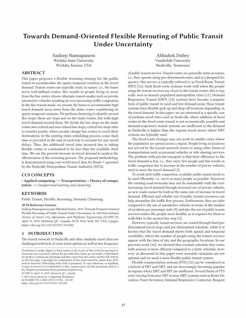
Figure 1 shows the scheduled route with critical and non-critical
bus stops along with possible flex routes. The flex stops indicated
in Figure 1 refer to the cluster centers obtained from the clustering
of spatial travel demand in Section 3.3. The notation for several
variables used in the problem formulation and their description are
provided in Table 1.
Figure 1: Conceptual scheduled route and possible flex route
options by substituting non-critical bus stops for flex stops
Table 1: Variable Notation and its description
Variable Description
Rik Scheduled route between consecutive critical stops Ci and Ck ,k = i + 1.
T (Ci ) Departure time at a critical stop Ci .T s (Ci ) Scheduled departure time at a critical stop Ci .
Fj
ikFlex route segment for Rik . Superscript j represents index of flexroute
Pik Represent either a segment of scheduled route or a flex route
D(Pik ) Number of people served on the segment PikC(Pik ) Additional congestion caused when a segment Pik is not catered
t (Pik ) Actual time taken to travel a segment Pikt s (Pik ) Time taken to travel a segment Pik according to the schedule
d (Pik ) Delay caused due to a route Pik compared against the scheduleroute Rik , d (Pik ) = t (Pik ) − t s (Rik )
t (s) Slack time available at the end point
ψ Radius of travel demand that a bus stop can cover
G1(D(Pik )) Loss Function associated with the people not serviced by the publictransit in segment Pik
G2(d (Pik )) Loss function associated with travel time delay in a segment PikNc Number of critical stops, including the start and end points
ηi Threshold departure time delay value at the i th critical stop
pi Threshold probability regarding the departure time delay at the
i th critical stop
Given the notation for several variables, the optimization prob-
lem for choosing the optimal flex route can be derived by solving
the following optimization problem.
Min
Nc−1∑i=1
E[w1 ×G2(d(Pik )) − (1 −w1) ×G1(D(Pik ))
]
subject to Pr( Nc−1∑
i=1
d(Pik ) ≥ ts)< γ
T (Ci ) > T (Cj ), ∀i > j
Pr (T (Ci ) −T s (Ci ) ≥ ηi ) < pi , i = 1 · · ·Nc
The overall minimization function is a weighted combination of
two loss functions: (1) people served, and (2) time delay in taking
a scheduled route or a flex route. The weights for the combina-
tion of the two objective functions (w1) and (1 −w1), and the cost
functions associated with the number of people not served and
time delay may be obtained from the local transit authority. The
weights (w1) and (1 − w1) represent the importance of the two
37
SCOPE’19, April 15, 2019, Montreal, QC, Canada Saideep Nannapaneni and Abhishek Dubey
objective functions; higherw1 represents more emphasis on mini-
mizing the travel delays while a lowerw1 value represents places
more emphasis on serving people. Since the travel demand and
time delay are uncertain, we optimize their expectation values. The
optimization is carried out under three constraints: (1) probabilis-
tic total delay constraint, (2) Ordering of the critical stops, and
(3) Time delay at the critical bus stops on the scheduled route. γrefers to the threshold probability value (0 ≤ γ ≤ 1), which can be
provided by the local transit authorities. Lower values of γ corre-
spond to tighter constraints while higher values of γ result in loose
constraints. The second constraint stipulates that the sequence of
critical bus stops remain the same as in the original schedule. The
third constraint specifies that the new departure time at the critical
stops should be within desired delays of the scheduled departure
time. ηi , i = 1, 2, 3 · · ·Nc represents the affordable departure de-
lay at a critical stop and pi , i = 1, 2, 3 · · ·Nc represents threshold
probability, i.e., the probability that the actual departure time at a
critical stop is greater than the scheduled departure time. Larger
time gaps between the scheduled and flex-route times can result in
disruptions of people’s travel plans.
To compute the number of people served, we define a parameter
ψ , which represents a radius around a bus stop (critical, non-critical
or flex). If a person lies within the ψ distance, then the person is
assumed to be served by the bus. Given a particular route (either
scheduled or fixed), the number of people that are served can be
computed, using the estimated spatial distribution of travel demand,
the flex stops andψ . An estimate of the time delay along a sched-
uled or a flex route is obtained using the Google Maps or equivalent
applications. The delay prediction is usually a point-value but in
reality, the actual delay may not match the predicted delay. There-
fore, we assume that the delay prediction is quantified through a
probability distribution. We use a lognormal distribution as it has
been previously used for modeling the travel time distribution [8].
The optimization is subject to a probabilistic constraint with respect
to the overall time delay, which is the aggregation of time delays
over all the individual segments. The optimization analysis helps
decide whether a flex route need to be taken as against a segment
the scheduled route. In case there are multiple possible flex routes,
the flex route that minimizes the overall loss function is selected.
Effectiveness of the Rerouting process: The next step after
performing the rerouting analysis is to decide if the new flex route
needs to be operated in place of the scheduled route. Rerouting
a scheduled route involves notifying people regarding the new
flex route. Frequent changes to the scheduled routes can cause
discomfort to regular passengers; therefore, we use the percent
increase in travel demand served on a flex route to quantify the
effectiveness of the rerouting process. If DF and DS represent the
total travel demand served on the flex and scheduled routes, then
the percent increase (denoted as PD ) in travel demand served on
the flex route is calculated as PD =DF−DS
DS× 100%.
We then define a threshold percentage Δ, and if PD > Δ, thenthe new flex route is operated else the scheduled route is operated.
The threshold Δ can be determined by the local transit authorities.
In this way, we determine if a flex or scheduled route needs to be
operated. The optimization formulation described above considers
the uncertainty in travel demand and travel time, and performs
Table 2: Departure delay parameters at the critical stops
Critical stop ID ηi (min) pi1 0.5 0.01
2 2 0.01
3 3 0.01
4 6 0.01
rerouting under a probabilistic constraint in the overall travel delay.
A common approach for solving such stochastic optimization prob-
lems is through Monte Carlo Sampling, where for each possible
flex route option, multiple realizations of the travel demand and
travel time are generated to evaluate the probabilistic objective and
constraint functions. For the sake of demonstration, we present the
implementation and results below considering only one realization
of travel time and travel demand.
4 IMPLEMENTATION AND RESULTS
Problem Parameters: For simplicity, we do not consider any
losses due to additional travel delay (G2(d(Pik )) in Table 1). Not
considering the loss due to additional travel delay signifies that
we are completely committed to accommodating as much travel
demand as possible under the slack time constraint.
We considered real transaction data occurring on several trips
taken on Route 7 between 9 am and 10 am, on every Monday in
October 2016. The γ parameter, which represents the delay thresh-
old is set to 1. This represents a stringent requirement that the
additional travel time should always be less than the available slack
time, which is assumed to be equal to 7 min. In this example, we
have four critical stops (including start and end stops), as shown
in Fig. 2. The departure delay parameters (ηi and pi , i = 1 to 4) aregiven in Table 2. The parameter, Δ, that represents the thresholdincrease in travel demand is assumed to be 10%.
Estimating Travel Demand:We use a combination of transac-
tion data from Route 7 and other nearby bus routes (21 bus routes in
total) also going to Music City Central available from the Nashville
MTA. For illustration, we assumed that 50% of travel demand to the
Music City Central use private transit modes (driving their own
vehicles or ride-sharing services), while the remaining use public
transit. Note that these numbers represent the proportions of travel
demand around Route 7, and do not represent the entire travel char-
acteristics in Nashville. The steps for simulating the travel demand
used for rerouting analysis is given below:
(1) Data pre-processing: The original transaction dataset ob-
tained from Nashville MTA had timestamp, vehicle, location
and route, but lacks some necessary information, such as
direction, trip, and stop. To extend the original transaction
data and obtain complete information of each transaction,
we pre-processed the dataset by linking the time stamp with
static schedule of Route 7. This helped us obtain detailed
information of every trip on Route 7.
(2) Data filtering: Transaction data is considered as valid travel
demand if the transaction happens within 1 mile from the
route and the transaction time is within a period that is
between 30 minutes before the time window starts and 30
minutes after the time window ends. MongoDB [6] was used
to store the transaction data as geospatial objects, which
enabled quick geographical query.
38
Towards Demand-Oriented Flexible Rerouting of Public Transit Under Uncertainty SCOPE’19, April 15, 2019, Montreal, QC, Canada
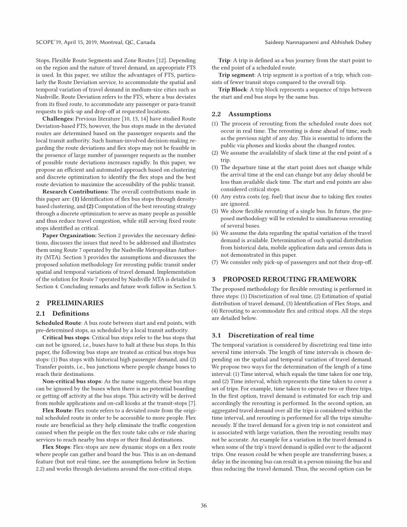
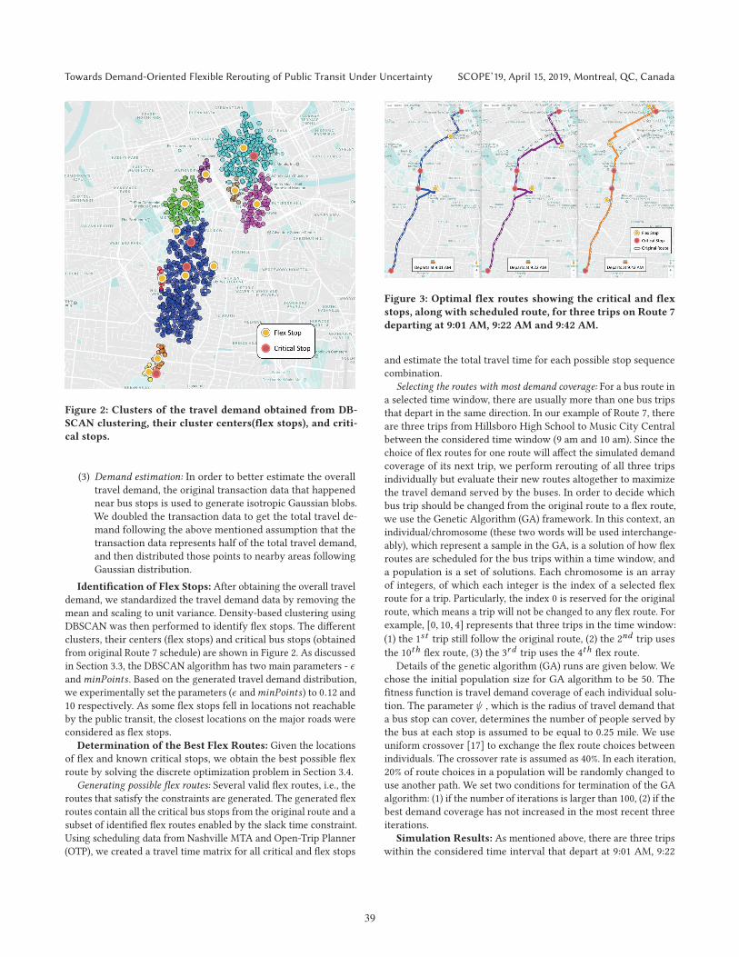
Figure 2: Clusters of the travel demand obtained from DB-
SCAN clustering, their cluster centers(flex stops), and criti-
cal stops.
(3) Demand estimation: In order to better estimate the overall
travel demand, the original transaction data that happened
near bus stops is used to generate isotropic Gaussian blobs.
We doubled the transaction data to get the total travel de-
mand following the above mentioned assumption that the
transaction data represents half of the total travel demand,
and then distributed those points to nearby areas following
Gaussian distribution.
Identification of Flex Stops: After obtaining the overall travel
demand, we standardized the travel demand data by removing the
mean and scaling to unit variance. Density-based clustering using
DBSCAN was then performed to identify flex stops. The different
clusters, their centers (flex stops) and critical bus stops (obtained
from original Route 7 schedule) are shown in Figure 2. As discussed
in Section 3.3, the DBSCAN algorithm has two main parameters - ϵandminPoints . Based on the generated travel demand distribution,
we experimentally set the parameters (ϵ andminPoints) to 0.12 and10 respectively. As some flex stops fell in locations not reachable
by the public transit, the closest locations on the major roads were
considered as flex stops.
Determination of the Best Flex Routes: Given the locations
of flex and known critical stops, we obtain the best possible flex
route by solving the discrete optimization problem in Section 3.4.
Generating possible flex routes: Several valid flex routes, i.e., the
routes that satisfy the constraints are generated. The generated flex
routes contain all the critical bus stops from the original route and a
subset of identified flex routes enabled by the slack time constraint.
Using scheduling data from Nashville MTA and Open-Trip Planner
(OTP), we created a travel time matrix for all critical and flex stops
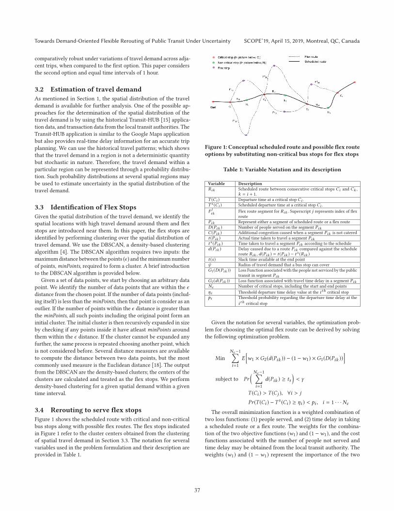
Figure 3: Optimal flex routes showing the critical and flex
stops, along with scheduled route, for three trips on Route 7
departing at 9:01 AM, 9:22 AM and 9:42 AM.
and estimate the total travel time for each possible stop sequence
combination.
Selecting the routes with most demand coverage: For a bus route in
a selected time window, there are usually more than one bus trips
that depart in the same direction. In our example of Route 7, there
are three trips from Hillsboro High School to Music City Central
between the considered time window (9 am and 10 am). Since the
choice of flex routes for one route will affect the simulated demand
coverage of its next trip, we perform rerouting of all three trips
individually but evaluate their new routes altogether to maximize
the travel demand served by the buses. In order to decide which
bus trip should be changed from the original route to a flex route,
we use the Genetic Algorithm (GA) framework. In this context, an
individual/chromosome (these two words will be used interchange-
ably), which represent a sample in the GA, is a solution of how flex
routes are scheduled for the bus trips within a time window, and
a population is a set of solutions. Each chromosome is an array
of integers, of which each integer is the index of a selected flex
route for a trip. Particularly, the index 0 is reserved for the original
route, which means a trip will not be changed to any flex route. For
example, [0, 10, 4] represents that three trips in the time window:
(1) the 1st trip still follow the original route, (2) the 2nd trip uses
the 10th flex route, (3) the 3rd trip uses the 4th flex route.
Details of the genetic algorithm (GA) runs are given below. We
chose the initial population size for GA algorithm to be 50. The
fitness function is travel demand coverage of each individual solu-
tion. The parameterψ , which is the radius of travel demand that
a bus stop can cover, determines the number of people served by
the bus at each stop is assumed to be equal to 0.25 mile. We use
uniform crossover [17] to exchange the flex route choices between
individuals. The crossover rate is assumed as 40%. In each iteration,
20% of route choices in a population will be randomly changed to
use another path. We set two conditions for termination of the GA
algorithm: (1) if the number of iterations is larger than 100, (2) if the
best demand coverage has not increased in the most recent three
iterations.
Simulation Results: As mentioned above, there are three trips
within the considered time interval that depart at 9:01 AM, 9:22
39
SCOPE’19, April 15, 2019, Montreal, QC, Canada Saideep Nannapaneni and Abhishek Dubey
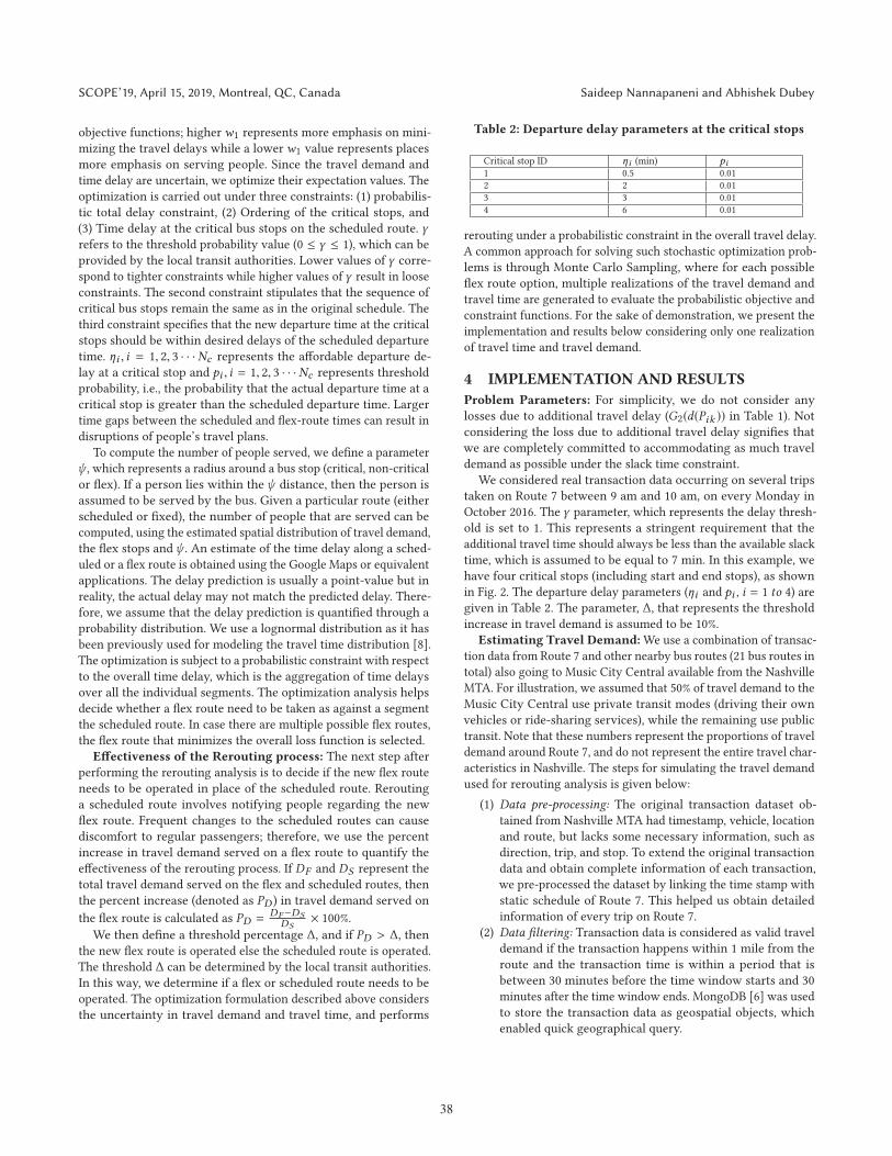
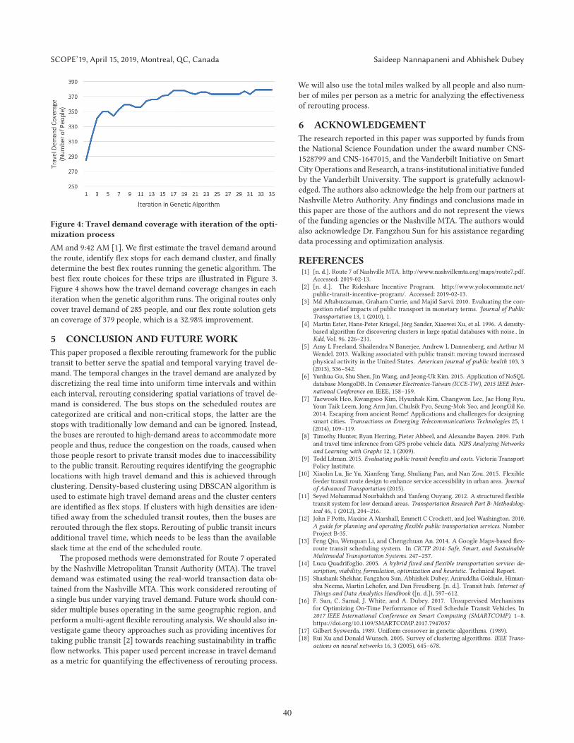
Figure 4: Travel demand coverage with iteration of the opti-
mization process
AM and 9:42 AM [1]. We first estimate the travel demand around
the route, identify flex stops for each demand cluster, and finally
determine the best flex routes running the genetic algorithm. The
best flex route choices for these trips are illustrated in Figure 3.
Figure 4 shows how the travel demand coverage changes in each
iteration when the genetic algorithm runs. The original routes only
cover travel demand of 285 people, and our flex route solution gets
an coverage of 379 people, which is a 32.98% improvement.
5 CONCLUSION AND FUTUREWORK
This paper proposed a flexible rerouting framework for the public
transit to better serve the spatial and temporal varying travel de-
mand. The temporal changes in the travel demand are analyzed by
discretizing the real time into uniform time intervals and within
each interval, rerouting considering spatial variations of travel de-
mand is considered. The bus stops on the scheduled routes are
categorized are critical and non-critical stops, the latter are the
stops with traditionally low demand and can be ignored. Instead,
the buses are rerouted to high-demand areas to accommodate more
people and thus, reduce the congestion on the roads, caused when
those people resort to private transit modes due to inaccessibility
to the public transit. Rerouting requires identifying the geographic
locations with high travel demand and this is achieved through
clustering. Density-based clustering using DBSCAN algorithm is
used to estimate high travel demand areas and the cluster centers
are identified as flex stops. If clusters with high densities are iden-
tified away from the scheduled transit routes, then the buses are
rerouted through the flex stops. Rerouting of public transit incurs
additional travel time, which needs to be less than the available
slack time at the end of the scheduled route.
The proposed methods were demonstrated for Route 7 operated
by the Nashville Metropolitan Transit Authority (MTA). The travel
demand was estimated using the real-world transaction data ob-
tained from the Nashville MTA. This work considered rerouting of
a single bus under varying travel demand. Future work should con-
sider multiple buses operating in the same geographic region, and
perform a multi-agent flexible rerouting analysis. We should also in-
vestigate game theory approaches such as providing incentives for
taking public transit [2] towards reaching sustainability in traffic
flow networks. This paper used percent increase in travel demand
as a metric for quantifying the effectiveness of rerouting process.
We will also use the total miles walked by all people and also num-
ber of miles per person as a metric for analyzing the effectiveness
of rerouting process.
6 ACKNOWLEDGEMENT
The research reported in this paper was supported by funds from
the National Science Foundation under the award number CNS-
1528799 and CNS-1647015, and the Vanderbilt Initiative on Smart
City Operations and Research, a trans-institutional initiative funded
by the Vanderbilt University. The support is gratefully acknowl-
edged. The authors also acknowledge the help from our partners at
Nashville Metro Authority. Any findings and conclusions made in
this paper are those of the authors and do not represent the views
of the funding agencies or the Nashville MTA. The authors would
also acknowledge Dr. Fangzhou Sun for his assistance regarding
data processing and optimization analysis.
REFERENCES[1] [n. d.]. Route 7 of Nashville MTA. http://www.nashvillemta.org/maps/route7.pdf.
Accessed: 2019-02-13.[2] [n. d.]. The Rideshare Incentive Program. http://www.yolocommute.net/
public-transit-incentive-program/. Accessed: 2019-02-13.[3] Md Aftabuzzaman, Graham Currie, and Majid Sarvi. 2010. Evaluating the con-
gestion relief impacts of public transport in monetary terms. Journal of PublicTransportation 13, 1 (2010), 1.
[4] Martin Ester, Hans-Peter Kriegel, Jörg Sander, Xiaowei Xu, et al. 1996. A density-based algorithm for discovering clusters in large spatial databases with noise.. InKdd, Vol. 96. 226–231.
[5] Amy L Freeland, Shailendra N Banerjee, Andrew L Dannenberg, and Arthur MWendel. 2013. Walking associated with public transit: moving toward increasedphysical activity in the United States. American journal of public health 103, 3(2013), 536–542.
[6] Yunhua Gu, Shu Shen, Jin Wang, and Jeong-Uk Kim. 2015. Application of NoSQLdatabase MongoDB. In Consumer Electronics-Taiwan (ICCE-TW), 2015 IEEE Inter-national Conference on. IEEE, 158–159.
[7] Taewook Heo, Kwangsoo Kim, Hyunhak Kim, Changwon Lee, Jae Hong Ryu,Youn Taik Leem, Jong Arm Jun, Chulsik Pyo, Seung-Mok Yoo, and JeongGil Ko.2014. Escaping from ancient Rome! Applications and challenges for designingsmart cities. Transactions on Emerging Telecommunications Technologies 25, 1(2014), 109–119.
[8] Timothy Hunter, Ryan Herring, Pieter Abbeel, and Alexandre Bayen. 2009. Pathand travel time inference from GPS probe vehicle data. NIPS Analyzing Networksand Learning with Graphs 12, 1 (2009).
[9] Todd Litman. 2015. Evaluating public transit benefits and costs. Victoria TransportPolicy Institute.
[10] Xiaolin Lu, Jie Yu, Xianfeng Yang, Shuliang Pan, and Nan Zou. 2015. Flexiblefeeder transit route design to enhance service accessibility in urban area. Journalof Advanced Transportation (2015).
[11] Seyed Mohammad Nourbakhsh and Yanfeng Ouyang. 2012. A structured flexibletransit system for low demand areas. Transportation Research Part B: Methodolog-ical 46, 1 (2012), 204–216.
[12] John F Potts, Maxine A Marshall, Emmett C Crockett, and Joel Washington. 2010.A guide for planning and operating flexible public transportation services. NumberProject B-35.
[13] Feng Qiu, Wenquan Li, and Chengchuan An. 2014. A Google Maps-based flex-route transit scheduling system. In CICTP 2014: Safe, Smart, and SustainableMultimodal Transportation Systems. 247–257.
[14] Luca Quadrifoglio. 2005. A hybrid fixed and flexible transportation service: de-scription, viability, formulation, optimization and heuristic. Technical Report.
[15] Shashank Shekhar, Fangzhou Sun, Abhishek Dubey, Aniruddha Gokhale, Himan-shu Neema, Martin Lehofer, and Dan Freudberg. [n. d.]. Transit hub. Internet ofThings and Data Analytics Handbook ([n. d.]), 597–612.
[16] F. Sun, C. Samal, J. White, and A. Dubey. 2017. Unsupervised Mechanismsfor Optimizing On-Time Performance of Fixed Schedule Transit Vehicles. In2017 IEEE International Conference on Smart Computing (SMARTCOMP). 1–8.https://doi.org/10.1109/SMARTCOMP.2017.7947057
[17] Gilbert Syswerda. 1989. Uniform crossover in genetic algorithms. (1989).[18] Rui Xu and Donald Wunsch. 2005. Survey of clustering algorithms. IEEE Trans-
![Efficient Energy Routing with connections Rerouting in ...1989/06/02 · optical spectrum management on the problem of routing and wavelength assignment [1-3], rerouting / optical](https://static.documents.pub/doc/80x56/60bbe452126f001e7f6854c2/efficient-energy-routing-with-connections-rerouting-in-19890602-optical.jpg)


