Towards efficient prospective detection of multiplespatio-temporal clusters

Braulio Veloso1, Andrea Iabrudi1, Thais Correa2

1 Computer Science Department2Statistics Department

Universidade Federal de Ouro Preto (UFOP) – Ouro Preto, MG – Brazil

{andrea.iabrudi,thaiscorrea}@iceb.ufop.br, brauliocic091@gmail.com

Abstract. In this paper we propose a novel technique to efficiently detect mul-tiple emergent clusters in a space-time point process. Emergent cluster detec-tion in large datasets is a ubiquitous task in any application area where fastresponse is crucial, like epidemic surveillance, criminology or social networksbehavior changing. Although different authors investigate aspects of efficientspatio-temporal cluster detection, they handle either multiple or prospective de-tection of spatio-temporal clusters. Our work concomitantly presents a solutionfor both aspects: prospective and multiple cluster efficient detection in spaceand time. Our results with synthetic data are very encouraging, since with awide range of parameters, we are able to detect multiple clusters in about 90%of the scenarios with very low type I and II errors (less than 2%), without in-creasing delay time.

1. IntroductionThis work presents a new method for accurate and computationally efficient prospectivedetection of multiple clusters in space-time event databases, suitable for intensive gene-rating processes. A spatio-temporal cluster is an aggregate of points that are groupedtogether in space and time with an abnormally high incidence, which has a low probabi-lity to have occurred by chance alone. A process that detects such a cluster at earlier stage– an emergent or live cluster – is called surveillance system [Hohle 2007]. Surveillancesystem development is a ubiquitous task in any application area where fast response iscrucial. These application areas include public health and safety surveillance, real lifeevent detection from social network data, traffic control, among others.

Spatio-temporal data is increasingly available as geo-tagged procedures are morepopular [Richardson 2013]. Geographic information system community are activelyproposing methods to tackle with many different issues [Oliveira and Baptista 2012]:storage, information recovery, ontologies and visualization methods specific for spatio-temporal data. In particular, specialized clustering is a promising and important areafor the GIScience and KDD communities [Bogorny and Shekhar 2010, Goodchild 2010].[?] classify spatio-temporal types in: ST Events, Geo-Referenced Variables, MovingObjects and Trajectories. Moving Objects and Trajectories are recent in GeographicInformation [Gudmundsson et al. 2012], while Geo-Referenced Variables are usual inData Mining applications [Birant and Kut 2007] and ST Event, in Computational Statis-tics [Kulldorff 2001]. Our method classifies as an early distance-based ST event clusteringdetection procedure.

Proceedings of XIV GEOINFO, November 24-27, 2013, Campos do Jordao, Brazil.

61

Epidemiology is traditionally a proficuous area for surveillance systems, asdisease outbreak detection is a crucial task, requiring very fast reaction from public agents.Through the years, many different methods have been proposed [Marshall et al. 2007,Tango et al. 2011], investigating alternative point process hypothesis, various clustershapes, and interaction of Spatio, Spatio-Temporal (ST) and Non-ST data. Usually, themethod’s quality is measured by the Type I (false clusters identification) and Type II (nodetection of true clusters) errors and, for prospective detection, the delay time (elapsedtime between the cluster start and its actual identification). There is no single winnermethod that applies for all situations and applications, and generally the underlying hy-pothesis are very different and sometimes restrictive. Besides that, recent increase in dataavailability strengthenes the need of computationally efficient approaches.

In our work, we identify whether there are one or more anomalous concentra-tions of point events in the very early stage. The underlying assumption is that the pointsare generated by a Poisson process, with rates that may vary both in space and time. Thespecific distribution parameters are directly estimated from the data, and may be heteroge-neous and non stationary, guaranteeing broad applicability. Furthermore, there is explicitcontrol of Type I error. Computational cost is controlled by considering only cylindricalclusters and using simple likelihood statistics to identify unexpected concentrations, asin [Li et al. 2011].

In a previous work [Veloso et al. 2012], we showed that our method is suitableto handle large volumes of spatio-temporal data to discover actual events from socialnetwork message. This work is a step towards bringing together Statistical Comput-ing and GIScience applications, by allowing existence of multiple clusters, which islikely when the generating process is intense. Detection of multiple clusters has beeninvestigated by spatial and spatial-temporal retrospective cluster detection community.In [Zhang et al. 2010], a sequential version of the spatial scan statistic procedure is ad-justed for the presence of other clusters in the study region, by sequential deletion of thepreviously detected clusters, much like as our approach. In [Li et al. 2011], the authorsconsider the existence of multiple clusters directly by the alternative hypothesis and showbetter power in terms of both rejecting the null hypothesis and accurately detecting the co-existing clusters. Both methods are not suitable to emergent detection and have significantcomputational cost. Adopting a graph-based strategy, [Demattei and Cucala 2010] iden-tify clusters by linking the events closest than a given distance and thus defining a graphassociated to the point process. The set of possible clusters is then restricted to windowsincluding the connected components of the graph. This allow detection of multiple, ar-bitrary shaped clusters with relatively efficiency. There is no extension for prospectivedetection, as far as we know.

Our main contribution in this paper is to extend the method in[Assuncao and Correa 2009] to identify multiple clusters, using a sequential strat-egy of deleting some events of already identified clusters. The proposed method isevaluated for a wide range of synthetic scenarios, simulating rare to intensive processes,where two spatially separated clusters are inserted. In this controlled setup, our resultsare very promising, with more than 93% of correct detections. We first present theoriginal method, followed by our extension to couple with multiple clusters. The metricsused to evaluate the method are detailed and results are then presented and discussed.

Proceedings of XIV GEOINFO, November 24-27, 2013, Campos do Jordao, Brazil.

62

Final remarks and possible future directions close the article.

2. MethodWe extended the method proposed by [Assuncao and Correa 2009] for detection of mul-tiple space-time clusters. In section 2.1, the original method, designed for an uniquespace-time cluster detection is briefly presented. We state our extension in section 2.2,proposing the algorithms for it.

2.1. Review: on line detection of an unique space-time cluster

Consider a point process observed in a three dimensional area A ⇥ (0, T ] where A rep-resents the space and (0, T ] is the time. The original method looks for a live space-timecluster with cylindric shape. The radius ⇢ of the circular base must be specified by theuser. The method consist on monitoring a simple statistic that doesn’t depend on themarginals space and time intensities of events. When this statistic exceeds a threshold themethod rings an alarm and the detected cluster is identified.

Events are sequentially observed at times t1, t2, . . . and they are processed as soonas they happen. The spatial coordinates for an event observed at time ti are (xi, yi). LetCk,n 2 A ⇥ (0, T ] be a cylinder with circular base spatially centered at (xk, yk). Theheight of Ck,n is given by tn � tk, where tn is the time of the last observed event. Notethat, considering tn as the current time, Ck,n is a live cylinder, since it reaches tn. LetN(Ck,n) be the number of events inside the cylinder Ck,n, we assume that it follows aPoisson distribution, N(Ck,n) ⇠ Poisson(µ(Ck,n)). The Poisson distribution is broadlyused in methods of cluster detection due to its suitability for modeling count data. If thereis no cluster, no space-time dependency exists, implying that space-time event intensity�(x, y, t) is separable and may be written as the product of the space and time marginalintensities:

�(x, y, t) = µ �s(x, y) �t(t), µ =

Z

A

Z

(0,T ]

�(x, y, t) dt dx dy.

However, if a cluster Ck,n emerges at time tk, dependency change in distributionis captured by a constant " > 0 such that

�(x, y, t) = µ �s(x, y) �t(t) (1 + "ICk,n

(x, y, t)) ,

where ICk,n

is an indicator function for (x, y, t) 2 Ck,n and " represents the intensityincrease inside the cluster. The excess " is a method parameter specified by the user.

The test statistic compares the null hypothesis of no cluster existence against alocalized cylindrical cluster alternative. Let L1 be the likelihood of the spacetime Poissonprocess when there is no cluster and let Lk be the likelihood of this same process whenthere is a cluster Ck,n, both for n observed events. The test statistic is the sum of thelikelihood ratio over all possibilities for the cylinder Ck,n:

Rn =

nX

k=1

Lk

L1=

nX

k=1

⇤k,n =

nX

k=1

(1 + ")N(Ck,n

)exp(�" µ(Ck,n)) .

Proceedings of XIV GEOINFO, November 24-27, 2013, Campos do Jordao, Brazil.

63

The method uses a non parametric estimate for the mean µ(Ck,n), as in practice itis unknown. Assuming that �(x, y, t) is separable, our method estimates this quantity by:

µ(Ck,n) =

N( B(k, ⇢)⇥ (0, tn] ) N( A⇥ (tk, tn] )

n,

where N( Bk,⇢ ⇥ (0, tn] ) is the number of events inside the circular base of cylinderCk,n irrespective of time, N(A ⇥ (tk, tn]) is the number of event between time tk and tnirrespective of space, and n is the total number of events.

When the test statistic exceeds a threshold A, the method rings an alarm indicatingthere is evidence of a live cluster. As the test statistic is a sum over all possible liveclusters, the estimate of the detected live cluster is the one with largest contribution to thetest statistic. That is, if Rn > A, then ⇤k⇤,n = max{⇤k,n, 1 k n} and the estimatedcluster is Ck⇤,n.

Assume that there is a cluster starting at time tk. If the test statistic exceeds thethreshold A at some time t < tk, then it is a false alarm. Otherwise, if threshold A isexceeded at time t > tk, it is a motivated alarm. Surveillance systems must address thetrade-off between fast detection and low false alarm rate. In our method, this is accom-plished by setting the threshold A to be equal to the desired value of the Average RunLength (ARL), the expected number of events before a false alarm. It ensures that, on av-erage, the user will wait at least A events before a false alarm, expressing user toleranceto wrong alerts.

2.2. Our extension for simultaneous space-time clusters

Now suppose we are using the method above and the alarm rings. It means there isevidence of a live cluster. In this case, is there evidence of a second live cluster? Whatabout a third live cluster? We answer these questions with our extension for the situationwhere more than one cluster start at the same time tk. The radius and the increase in theintensity for all clusters are the same: ⇢ and ", respectively. For simplicity, we describethe extension for two clusters, but it can be generalized for any number of simultaneousclusters.

In the original method with a threshold A, consider there is an alarm at time tn.The estimated cluster is Ck⇤,n. Our sequential approach consists in deleting the excessof events inside Ck⇤,n in a random way and reapplying the original method to this newreduced database. The excess of events is the difference between the observed and theexpected number of events: �(Ck⇤,n) = N(Ck⇤,n)� µk⇤,n .

After deletion of the exceeding events, we have a reduced database. We thenevaluate the test statistic at the current time tn for this new reduced database. We willrefer to the statistic for the reduced database as R0

n to distinguish from Rn. Since weartificially erased the cluster Ck⇤,n, if R0

n is more than a new threshold it is due to asecond live cluster, it is hoping one different from Ck⇤,n. The estimate for this secondcluster is the one with largest contribution to the test statistic R0

n, just as in the originalmethod. The new threshold A0 is equal to the old one, except for the events we delete:A0

= A��(Ck⇤,n).

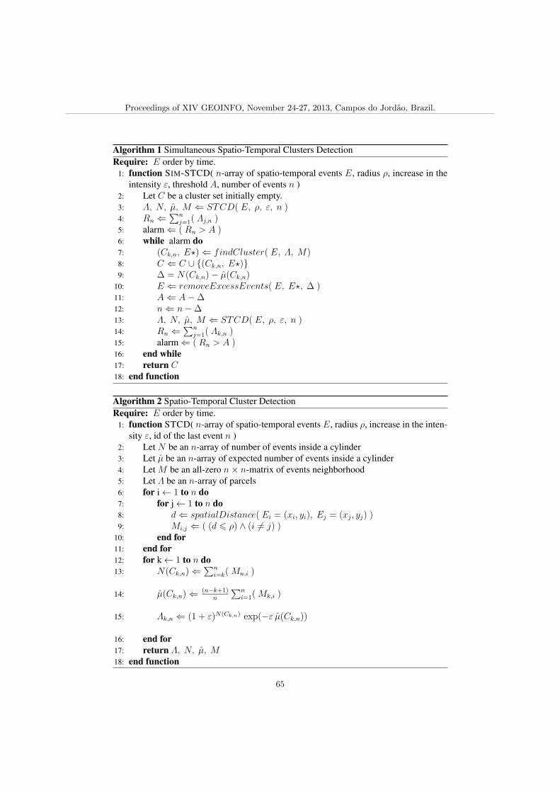
Algorithms 1, 2, 3 and 4 show our extension.

Proceedings of XIV GEOINFO, November 24-27, 2013, Campos do Jordao, Brazil.

64

Algorithm 1 Simultaneous Spatio-Temporal Clusters DetectionRequire: E order by time.

1: function SIM-STCD( n-array of spatio-temporal events E, radius ⇢, increase in theintensity ", threshold A, number of events n )

2: Let C be a cluster set initially empty.3: ⇤, N, µ, M ( STCD( E, ⇢, ", n )

4: Rn (Pn

j=1( ⇤j,n )

5: alarm( ( Rn > A )

6: while alarm do7: (Ck,n, E?)( findCluster( E, ⇤, M)

8: C ( C [ {(Ck,n, E?)}9: � = N(Ck,n)� µ(Ck,n)

10: E ( removeExcessEvents( E, E?, � )

11: A( A��

12: n( n��

13: ⇤, N, µ, M ( STCD( E, ⇢, ", n )

14: Rn (Pn

j=1( ⇤k,n )

15: alarm( ( Rn > A )

16: end while17: return C18: end function

Algorithm 2 Spatio-Temporal Cluster DetectionRequire: E order by time.

1: function STCD( n-array of spatio-temporal events E, radius ⇢, increase in the inten-sity ", id of the last event n )

2: Let N be an n-array of number of events inside a cylinder3: Let µ be an n-array of expected number of events inside a cylinder4: Let M be an all-zero n⇥ n-matrix of events neighborhood5: Let ⇤ be an n-array of parcels6: for i 1 to n do7: for j 1 to n do8: d( spatialDistance( Ei = (xi, yi), Ej = (xj, yj) )

9: Mi,j ( ( (d 6 ⇢) ^ (i 6= j) )

10: end for11: end for12: for k 1 to n do13: N(Ck,n)(

Pni=k( Mn,i )

14: µ(Ck,n)( (n�k+1)n

Pni=1( Mk,i )

15: ⇤k,n ( (1 + ")N(Ck,n

)exp(�" µ(Ck,n))

16: end for17: return ⇤, N, µ, M18: end function

Proceedings of XIV GEOINFO, November 24-27, 2013, Campos do Jordao, Brazil.

65

Algorithm 3 function findCluster1: function FINDCLUSTER( n-array of spatio-temporal events E, parcel’s array ⇤,

events neighborhood matrix M )2: ⇤k⇤,n (MAX{⇤k,n, 1 6 k 6 n}3: Then, let Ck⇤,n be the cylinder that define the cluster found beginning in event k⇤

and finishing in time of event n4: Let E? be a dataset empty5: E? ( E? [ {Ek⇤}6: for i (k ⇤+1) to n do . note: As data are ordered by time, only the events

greater than k⇤ can be inside the cylinder Ck⇤,n.7: if event i is a k⇤ neighbor, ie., Mi,k⇤ = 1

8: then E? ( E? [ {Ei}9: end if

10: end for11: return ( Ck⇤,n, E?

)

12: end function

Algorithm 4 procedure removeExcessEvents1: procedure REMOVEEXCESSEVENTS( spatio-temporal events dataset E, spatio-

temporal events sub-dataset E?, number of events in excess � )2: Let E 0 be an empty dataset3: for i 1 to � do4: Sort an event Ek of E?, always a different one.5: E 0 ( E 0 [ {Ek}6: end for7: E ( E � E 0

8: end procedure

3. Evaluation metrics

We defined some metrics to evaluate the method for simulated databases. We firstdescribe these metrics when an unique cluster is present. In this case, we analyzed thepercentages of No Alarm, Incorrect Alarm, and Correct Alarm. A No Alarm occurs whenRi < A for all i = 1, . . . , n, where n is the total number of events in the database. AnIncorrect Alarm occurs when Ri > A for some i = 1, . . . , n and the events set of theestimated cluster has no intersection with the events set of the real one. A Correct Alarmhappens when Ri > A for some i = 1, . . . , n and the events set of estimated clusterhas any intersection with the events set of real one. For each database we used, we letthe time moves forward until a Correct Alarm and record the total number of differentalarms. If Ri > A, Ri+1 < A, Ri+2 > A, then the alarms at times i and i + 2 wasconsidered as different alarms. When Ri > A, Ri+1 > A and the estimated clusters attimes i and i + 1 are the same, we considered the alarms at times i and i + 1 as the samealarm. If Ri > A, Ri+1 > A and the estimated clusters at time i and i + 1 are not thesame, we considered the alarms at times i and i + 1 as different alarms. We consider theestimated clusters as the same if the distance between their centers is greater than 2⇢.

Proceedings of XIV GEOINFO, November 24-27, 2013, Campos do Jordao, Brazil.

66

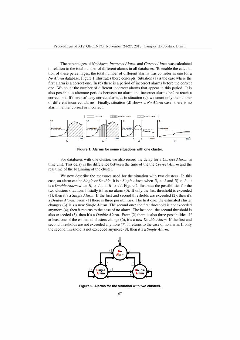
The percentages of No Alarm, Incorrect Alarm, and Correct Alarm was calculatedin relation to the total number of different alarms in all databases. To enable the calcula-tion of these percentages, the total number of different alarms was consider as one for aNo Alarm database. Figure 1 illustrates these concepts. Situation (a) is the case where thefirst alarm is a correct one. In (b) there is a period of incorrect alarms before the correctone. We count the number of different incorrect alarms that appear in this period. It isalso possible to alternate periods between no alarm and incorrect alarms before reach acorrect one. If there isn’t any correct alarm, as in situation (c), we count only the numberof different incorrect alarms. Finally, situation (d) shows a No Alarm case: there is noalarm, neither correct or incorrect.

Figure 1. Alarms for some situations with one cluster.

For databases with one cluster, we also record the delay for a Correct Alarm, intime unit. This delay is the difference between the time of the the Correct Alarm and thereal time of the beginning of the cluster.

We now describe the measures used for the situation with two clusters. In thiscase, an alarm can be Single or Double. It is a Single Alarm when Ri > A and R0

i < A0; itis a Double Alarm when Ri > A and R0

i > A0. Figure 2 illustrates the possibilities for thetwo clusters situation. Initially it has no alarm (0). If only the first threshold is exceeded(1), then it’s a Single Alarm. If the first and second thresholds are exceeded (2), then it’sa Double Alarm. From (1) there is three possibilities. The first one: the estimated clusterchanges (3), it’s a new Single Alarm. The second one: the first threshold is not exceededanymore (4), then it returns to the case of no alarm. The last one: the second threshold isalso exceeded (5), then it’s a Double Alarm. From (2) there is also three possibilities. Ifat least one of the estimated clusters change (6), it’s a new Double Alarm. If the first andsecond thresholds are not exceeded anymore (7), it returns to the case of no alarm. If onlythe second threshold is not exceeded anymore (8), then it’s a Single Alarm.

Figure 2. Alarms for the situation with two clusters.

Proceedings of XIV GEOINFO, November 24-27, 2013, Campos do Jordao, Brazil.

67

A Single Alarm can be Correct or Incorrect. A Single Alarm is Single CorrectAlarm if the estimated cluster has any intersection with one of the two real clusters, namedhere C1 and C2. If the estimated cluster has no intersection with C1 and no intersectionwith C2 it is a Single Incorrect Alarm. A Double Alarm can be Correct, Incorrect orHalf-Correct. A Double Correct Alarm occurs when one of the estimated clusters hasany intersection with C1 and the other estimated cluster has any intersection with C2.A Double Incorrect Alarm occurs the estimated clusters has no intersection with bothC1 and C2. Finally, it is a Double Half-Correct Alarm when only one of the estimatedclusters has any intersection with C1 or C2.

For each database with two clusters, we let the time moves forward until a DoubleCorrect Alarm and record the total number of different alarms. We analyzed the percent-ages of No Alarm, Incorrect Alarm, Incomplete Alarm, and Complete Alarm in relationto the total number of different alarms in all databases. Again, to enable the calculationof these percentages, the total number of different alarms was consider as one for a NoAlarm database. Here, Single Incorrect Alarm and Double Incorrect Alarm were bothconsidered as Incorrect Alarm. A Complete Alarm is a Double Correct Alarm. A SingleCorrect Alarm is an Incomplete Alarm. One Double Half-Correct Alarm represents 1/2Incorrect Alarm and 1/2 Incomplete Alarm.

4. Results

In this section we present the results we obtained applying both the original method andour extension to artificial (simulated) data. The original method was applied to databaseswith an unique cluster and the extension was applied to databases with two simultaneousclusters. We first describe the artificial databases we used in subsection 4.1 and then showthe results in the following subsections.

4.1. Simulated databases

In all databases we considered a 10⇥10-square as the space area and the the time rangingfrom 0 to 10. We used four different values for the spatial radius ⇢ : 0.5, 1.0, 1.5, 2.0. Forthe increase in the intensity inside the cluster " we tried three different values: 1, 3, 10.All clusters finish at time 10. We also varied the time the cluster emerges. We used 5, 7, 8for this initial time. In case of two clusters, time, radius ⇢ and the excess " are variedequality for both clusters. The clusters’ centers are distant by at least 4⇢, guaranteeingthat no cluster candidate intersects both of them simultaneously. In subsections 4.2 and4.3 the true values for ⇢ and " was used as input for these parameters. The threshold forthe alarm was always set as the total number of event in the database.

For of each combination of ⇢, " and initial time, we generated 100 databases.Figure 3 presents examples for database’s cases with one and two clusters. We show thesimulations results in the following subsections. The initial time of the cluster provednot to be significant, and then we show here the average of each measure for the threedifferent values we tried for this time. We also disregard the results for the combinations⇢ = 0.5, " = 1 and ⇢ = 2.0, " = 10, since the method proved to be inadequate in theseextremes.

Proceedings of XIV GEOINFO, November 24-27, 2013, Campos do Jordao, Brazil.

68

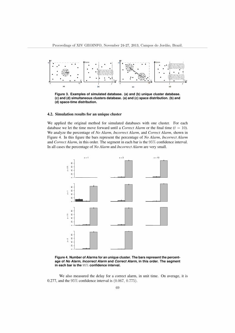
Figure 3. Examples of simulated database. (a) and (b) unique cluster database.(c) and (d) simultaneous clusters database. (a) and (c) space distribution. (b) and(d) space-time distribution.

4.2. Simulation results for an unique cluster

We applied the original method for simulated databases with one cluster. For eachdatabase we let the time move forward until a Correct Alarm or the final time (t = 10).We analyze the percentage of No Alarm, Incorrect Alarm, and Correct Alarm, shown inFigure 4. In this figure the bars represent the percentage of No Alarm, Incorrect Alarmand Correct Alarm, in this order. The segment in each bar is the 95% confidence interval.In all cases the percentage of No Alarm and Incorrect Alarm are very small.

02

04

06

08

0

! = 1

" =

0.5

! = 3 ! = 10

02

04

06

08

0

" =

1

02

04

06

08

0

" =

1.5

02

04

06

08

0

" =

2

Figure 4. Number of Alarms for an unique cluster. The bars represent the percent-age of No Alarm, Incorrect Alarm and Correct Alarm, in this order. The segmentin each bar is the 95% confidence interval.

We also measured the delay for a correct alarm, in unit time. On average, it is0.277, and the 95% confidence interval is (0.067, 0.775).

Proceedings of XIV GEOINFO, November 24-27, 2013, Campos do Jordao, Brazil.

69

4.3. Simulation results for simultaneous clusters

We applied our extension for simulated databases with two simultaneous clusters, C1 andC2. For each database we let the time move forward until a Double Correct Alarm or thefinal time (t = 10) and count the number of distinct alarms per case into database. Theresults are shown in Figure 5. In this figure the bars represent the percentage of No Alarm,Incorrect Alarm, Incomplete Alarm and Complete Alarm, in this order. The segment ineach bar is the 95% confidence interval. The percentage of No Alarm and Incorrect Alarmare always very small, as in the case of an unique cluster.

02

04

06

08

0

! = 1

" =

0.5

! = 3 ! = 10

02

04

06

08

0

" =

1

02

04

06

08

0

" =

1.5

02

04

06

08

0

" =

2

Figure 5. Number of Alarms for two clusters. The bars represent the percent-age of No Alarm, Incorrect Alarm, Incomplete Alarm and Complete Alarm, in thisorder. The segment in each bar is the 95% confidence interval.

Figure 6 shows the delay for both the cases with one cluster and two simultaneousclusters. The first bar represents the delay for a Correct Alarm when there is an uniquecluster (Delay 1). The second, third and fourth bars show the delay when there is twosimultaneous clusters. These bars represents, in this order, the delay until: the first CorrectAlarm (Delay Min), the detection of cluster C1 (Delay C1), the detection of cluster C2

(Delay C2), and a Double Correct Alarm (Delay Double). The segment in each bar isthe 95% confidence band: percentiles 2.5% and 97.5%. We did not found significantdifference for the average delay between Delay 1 and Delay Min. It means that, theextension for multiple clusters detects one cluster as fast as the original method. Asexpected, there is also no significant difference for the average delay between Delay C1and Delay C2. For all others combinations we found significant difference for the averagedelay. Note that, on average, Delay Double is usually more than Delay C1 and Delay C2and the percentage of Incomplete Alarm is always more than the percentage of Complete

Proceedings of XIV GEOINFO, November 24-27, 2013, Campos do Jordao, Brazil.

70

Alarm. It’s means: even before a Double Correct Alarm, our extension detects bothclusters in different alarms (Single Correct Alarms).

Independent of the number of alarms, on average, our extension reached a Com-plete Alarm in 88.2% of cases into database, while 10.6% of cases it only identifies onecluster of two expected (Incomplete Alarms) all the time. In 0.2% of cases have onlyIncorrect Alarms and 1% of cases have No Alarm.

0.0

1.0

2.0

3.0

! = 1

" =

0.5

! = 3 ! = 10

0.0

1.0

2.0

3.0

" =

1

0.0

1.0

2.0

3.0

" =

1.5

0.0

1.0

2.0

3.0

" =

2

Figure 6. Delays in time unit. The segment in each bar is the 95% confidenceband for: Correct Alarm for one cluster case, first Correct Alarm for two cluster

case, detection of cluster C1, detection of cluster C2, and Double Correct Alarm.

5. Final considerationsSimulation results in the previous section show that our extension for multiple cluster isquite satisfactory for spatially separate clusters. It detects one of the multiple clustersas fast as the original method. The percentage of detection for both clusters is around88%, and the delay is reasonably small. These are initial results, evaluating our methodcapability of detecting simultaneous clusters with respect to the original one.

Here we took ⇢ and " parameters to be exactly their true values on datasets.The impact of changing these parameters was evaluated for the original methodin [Assuncao and Correa 2009]. The same should be done for the extension for multipleclusters in a future work, as well as the application of the extension to real data. Other fu-ture direction is to compare our approach to others, establishing its relative efficiency andeffectiveness. Important issues to be considered hereafter are the automatic calibrationfor these parameters and removing the restriction on the cylindrical shape of the clusters,allowing for arbitrary shaped ones.

Proceedings of XIV GEOINFO, November 24-27, 2013, Campos do Jordao, Brazil.

71

ReferencesAssuncao, R. and Correa, T. (2009). Surveillance to detect emerging space-time clusters.

Comput. Stat. Data Anal., 53(8):2817–2830.

Birant, D. and Kut, A. (2007). ST-DBSCAN: An algorithm for clustering spatial–temporal data. Data & Knowledge Engineering, 60(1):208–221.

Bogorny, V. and Shekhar, S. (2010). Spatial and Spatio-temporal Data Mining. In DataMining (ICDM), 2010 IEEE 10th International Conference on, pages 1217–1217.

Demattei, C. and Cucala, L. (2010). Multiple spatio-temporal cluster detection for caseevent data: an ordering-based approach. Communications in Statistics-Theory andMethods, 40(2):358–372.

Goodchild, M. F. (2010). Twenty years of progress: GIScience in 2010. Journal of SpatialInformation Science, (1):3–20.

Gudmundsson, J., Laube, P., and Wolle, T. (2012). Computational Movement Analysis. InKresse, W. and Danko, D. M., editors, Springer Handbook of Geographic Information,pages 423–438. Springer Berlin Heidelberg.

Hohle, M. (2007). surveillance: An R package for the monitoring of infectious diseases.Computational Statistics, 22:571–582.

Kulldorff, M. (2001). Prospective time periodic geographical disease surveillance usinga scan statistic. Journal of the Royal Statistical Society, Series A, 164:61–72.

Li, X.-Z., Wang, J.-F., Yang, W.-Z., Li, Z.-J., and Lai, S.-J. (2011). A spatial scan statisticfor multiple clusters. Mathematical biosciences, 233(2):135–142.

Marshall, J. B., Spitzner, B. D., and Woodall, W. H. (2007). Use of the local Knox statisticfor the prospective monitoring of disease occurrences in space and time. Statistics inMedicine, 26:1579–1593.

Oliveira, M. G. d. and Baptista, C. d. S. (2012). GeoSTAT: A system for visualiza-tion, analysis and clustering of distributed spatiotemporal data. In Proceedings XIIIGEOINFO,, pages 108–119.

Richardson, D. B. (2013). Real-Time Space–Time Integration in GIScience and Geogra-phy. Annals of the Association of American Geographers, 103(5):1062–1071.

Tango, T., Takahashi, K., and Kohriyamma, K. (2011). A space-time scan statistic fordetecting emerging outbreaks. Biometrics, 67:106–115.

Veloso, B. M., Iabrudi, A. I., and Correa, T. R. (2012). Localizacao em tempo real deacontecimentos atraves de vigilancia espaco-temporal de microblogs. page 12. IXEncontro Nacional de Inteligencia Artificial.

Zhang, Z., Assuncao, R., and Kulldorff, M. (2010). Spatial scan statistics adjusted formultiple clusters. Journal of Probability and Statistics, 2010.

Proceedings of XIV GEOINFO, November 24-27, 2013, Campos do Jordao, Brazil.

72