Towards the solution of large-scale nonlinear SDP problems Michal Ko ˇ cvara and Michael Stingl UTIA AV ˇ CR Prague and University of Erlangen-N¨ urnberg Towards the solution of large-scale nonlinear SDP problems – p.1/20
Transcript
Towards the solution oflarge-scale nonlinear SDP problems
Michal Kocvara and Michael Stingl
UTIA AV CR Prague and University of Erlangen-Nurnberg
Towards the solution of large-scale nonlinear SDP problems – p.1/20
Background
Can we use iterative methods (CG, QMR) to the solution of Newtonsystems coming from penalty/barrier methods applied to NLP —instead of Cholesky factorization?
Yes, but. . .
Towards the solution of large-scale nonlinear SDP problems – p.2/20
Background
Can we use iterative methods (CG, QMR) to the solution of Newtonsystems coming from penalty/barrier methods applied to NLP —instead of Cholesky factorization?
Yes, but. . .
Sparse Cholesky often very efficient (BUT: dense columns)
Condition number of the system increases
NO GENERAL PRECONDITIONER
Towards the solution of large-scale nonlinear SDP problems – p.2/20
Background
Can we use iterative methods (CG, QMR) to the solution of Newtonsystems coming from penalty/barrier methods applied to NLP —instead of Cholesky factorization?
Yes, but. . .
Can we use iterative methods (CG, QMR) to the solution of Newtonsystems coming from penalty/barrier methods applied to SDP —instead of Cholesky factorization?Hmmm. . .
2 n2 ) for sparse data matrices(K . . . max. number of nonzeros in Ai, i = 1, . . . , n)
Complexity of augm. Lagrangian evaluation - linear SDP:
O(m3A
) for dense data matrices
O(m2A
κ) for sparse data matrices(κ . . . max. number of nonzeros in Li, (Ai − I) = LiL
Ti ,
i = 1, . . . , n)
Complexity of Cholesky algorithm - linear SDP:
O ( n
3 ) for dense Hessians
O ( n
2 .··· ) for sparse Hessians
Towards the solution of large-scale nonlinear SDP problems – p.7/20
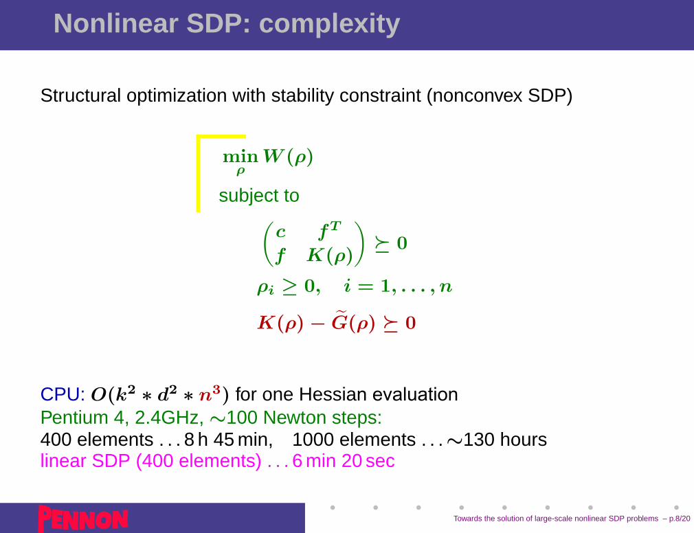
Nonlinear SDP: complexity
Structural optimization with stability constraint (nonconvex SDP)
minρ
W (ρ)
subject to(
c fT
f K(ρ)
)� 0
ρi ≥ 0, i = 1, . . . , n
K(ρ) − G(ρ) � 0
Towards the solution of large-scale nonlinear SDP problems – p.8/20
kocvara
min � W(ρ) subject to �c fT f K(ρ)� � 0 ρi ≥ 0, i = 1, . . . , n K(ρ) − e G(ρ) � 0
Nonlinear SDP: complexity
Structural optimization with stability constraint (nonconvex SDP)
minρ
W (ρ)
subject to(
c fT
f K(ρ)
)� 0
ρi ≥ 0, i = 1, . . . , n
K(ρ) − G(ρ) � 0
CPU: O ( k
2 ∗ d2 ∗ n3 ) for one Hessian evaluation
Towards the solution of large-scale nonlinear SDP problems – p.8/20
kocvara
min � W(ρ) subject to �c fT f K(ρ)� � 0 ρi ≥ 0, i = 1, . . . , n K(ρ) − e G(ρ) � 0
Nonlinear SDP: complexity
Structural optimization with stability constraint (nonconvex SDP)
minρ
W (ρ)
subject to(
c fT
f K(ρ)
)� 0
ρi ≥ 0, i = 1, . . . , n
K(ρ) − G(ρ) � 0
CPU: O ( k
2 ∗ d2 ∗ n3 ) for one Hessian evaluationPentium 4, 2.4GHz, ∼100 Newton steps:400 elements . . . 8 h 45 min, 1000 elements . . . ∼130 hours
Towards the solution of large-scale nonlinear SDP problems – p.8/20
kocvara
min � W(ρ) subject to �c fT f K(ρ)� � 0 ρi ≥ 0, i = 1, . . . , n K(ρ) − e G(ρ) � 0
Nonlinear SDP: complexity
Structural optimization with stability constraint (nonconvex SDP)
minρ
W (ρ)
subject to(
c fT
f K(ρ)
)� 0
ρi ≥ 0, i = 1, . . . , n
K(ρ) − G(ρ) � 0
CPU: O ( k
2 ∗ d2 ∗ n3 ) for one Hessian evaluationPentium 4, 2.4GHz, ∼100 Newton steps:400 elements . . . 8 h 45 min, 1000 elements . . . ∼130 hourslinear SDP (400 elements) . . . 6 min 20 sec
Towards the solution of large-scale nonlinear SDP problems – p.8/20
kocvara
min � W(ρ) subject to �c fT f K(ρ)� � 0 ρi ≥ 0, i = 1, . . . , n K(ρ) − e G(ρ) � 0
Motivation for CG
Use iterative solvers to improve:
Complexity of Cholesky algorithm - linear SDP:
O ( n
3 ) for dense Hessians → O ( n
2 )
O ( n
2 .··· ) for sparse Hessians → O ( n
2 )
Towards the solution of large-scale nonlinear SDP problems – p.9/20
kocvara
Use iterative solvers to improve:
Motivation for CG
Use iterative solvers to improve:
Complexity of Cholesky algorithm - linear SDP:
O ( n
3 ) for dense Hessians → O ( n
2 )
O ( n
2 .··· ) for sparse Hessians → O ( n
2 )
. . . too ambicious?
Complexity of Hessian assembling - nonlinear SDP:
O ( n
3 ) for dense data matrices
. . . using approximate Hessian-vector products
Towards the solution of large-scale nonlinear SDP problems – p.9/20
kocvara
Use iterative solvers to improve:
Iterative algorithms
Conjugate Gradient method for Hd = −g, H ∈ Sn+
. . .
. . .y = Hx complexity O(n2). . .. . .
Exact arithmetics: “convergence” in n steps
→ overall complexity O(n3)
Towards the solution of large-scale nonlinear SDP problems – p.10/20
kocvara
. . . . . . y = Hx . . . . . .
Iterative algorithms
Conjugate Gradient method for Hd = −g, H ∈ Sn+
. . .
. . .y = Hx complexity O(n2). . .. . .
Exact arithmetics: “convergence” in n steps
→ overall complexity O(n3)
Praxis: may be much worse (ill-conditioned problems)
Towards the solution of large-scale nonlinear SDP problems – p.10/20
kocvara
. . . . . . y = Hx . . . . . .
Iterative algorithms
Conjugate Gradient method for Hd = −g, H ∈ Sn+
. . .
. . .y = Hx complexity O(n2). . .. . .
Exact arithmetics: “convergence” in n steps
→ overall complexity O(n3)
Praxis: may be much worse (ill-conditioned problems)Praxis: may be much better → preconditioning
Convergence theory: number of iterations depends on
condition number
distribution of eigenvalues
Towards the solution of large-scale nonlinear SDP problems – p.10/20
Iterative algorithms
Conjugate Gradient method for Hd = −g, H ∈ Sn+
. . .
. . .y = Hx complexity O(n2). . .. . .
Exact arithmetics: “convergence” in n steps
→ overall complexity O(n3)
Praxis: may be much worse (ill-conditioned problems)Praxis: may be much better → preconditioning
Convergence theory: number of iterations depends on
condition number
distribution of eigenvalues
Preconditioning: solve M−1Hd = M−1g with M ≈ H−1
Towards the solution of large-scale nonlinear SDP problems – p.10/20
Conditioning of Hessian
Solve Hd = −g, H Hessian of
F (x, u, U, p, P ) = f(x) + 〈U, ΦP (A(x))〉SmA
Condition number depends on P
Example: problem Theta2 from SDPLIB (n = 498)
0 50 100 150 200 250 300 350 400 450500
-0.5
0
0.5
1
1.5
2
2.5
0 50 100 150 200 250 300 350 400 450500
-6
-5
-4
-3
-2
-1
0
1
2
3
κ0 = 394 κopt = 4.9 · 107
Towards the solution of large-scale nonlinear SDP problems – p.11/20
Theta2 from SDPLIB ( n = 498)
0 50 100 150 200 250 300 350 400 450500
-0.5
0
0.5
1
1.5
2
2.5
0 50 100 150 200 250 300 350 400 450500
-6
-5
-4
-3
-2
-1
0
1
2
3
Behaviour of CG: testing ‖Hd + g‖/‖g‖
0 2 4 6 8 10 12 1416
-10
-8
-6
-4
-2
0
2
0 100 200 300 400 500 600 700 800 9001000
-3
-2.5
-2
-1.5
-1
-0.5
0
0.5
1
Towards the solution of large-scale nonlinear SDP problems – p.12/20
Theta2 from SDPLIB ( n = 498)
0 50 100 150 200 250 300 350 400 450500
-0.5
0
0.5
1
1.5
2
2.5
0 50 100 150 200 250 300 350 400 450500
-6
-5
-4
-3
-2
-1
0
1
2
3
Behaviour of QMR: testing ‖Hd + g‖/‖g‖
0 2 4 6 8 10 12 1416
-10
-8
-6
-4
-2
0
2
0 100 200 300 400 500 600 700 800 9001000
-3.5
-3
-2.5
-2
-1.5
-1
-0.5
0
Towards the solution of large-scale nonlinear SDP problems – p.12/20
Theta2 from SDPLIB ( n = 498)
0 50 100 150 200 250 300 350 400 450500
-0.5
0
0.5
1
1.5
2
2.5
0 50 100 150 200 250 300 350 400 450500
-6
-5
-4
-3
-2
-1
0
1
2
3
QMR: effect of preconditioning (for small P )
0 100 200 300 400 500 600 700 800 9001000
-3.5
-3
-2.5
-2
-1.5
-1
-0.5
0
0 100 200 300 400 500 600 700 800 9001000
-7
-6
-5
-4
-3
-2
-1
0
Towards the solution of large-scale nonlinear SDP problems – p.12/20
Control3 from SDPLIB ( n = 136)
0 20 40 60 80 100 120140
2
3
4
5
6
7
8
9
10
11
0 20 40 60 80 100 120140
-8
-6
-4
-2
0
2
4
6
κ0 = 3.1 · 108 κopt = 7.3 · 1012
Towards the solution of large-scale nonlinear SDP problems – p.13/20
Control3 from SDPLIB ( n = 136)
0 20 40 60 80 100 120140
2
3
4
5
6
7
8
9
10
11
0 20 40 60 80 100 120140
-8
-6
-4
-2
0
2
4
6
Behaviour of CG: testing ‖Hd + g‖/‖g‖
0 50 100 150 200250
300-10
-8
-6
-4
-2
0
2
4
0 100 200 300 400 500 600 700 800 9001000
0.5
1
1.5
2
2.5
3
3.5
4
Towards the solution of large-scale nonlinear SDP problems – p.13/20
Control3 from SDPLIB ( n = 136)
0 20 40 60 80 100 120140
2
3
4
5
6
7
8
9
10
11
0 20 40 60 80 100 120140
-8
-6
-4
-2
0
2
4
6
Behaviour of QMR: testing ‖Hd + g‖/‖g‖
0 50 100 150 200250
300-10
-9
-8
-7
-6
-5
-4
-3
-2
-1
0
0 100 200 300 400 500 600 700 800 9001000
-0.18
-0.16
-0.14
-0.12
-0.1
-0.08
-0.06
-0.04
-0.02
0
Towards the solution of large-scale nonlinear SDP problems – p.13/20
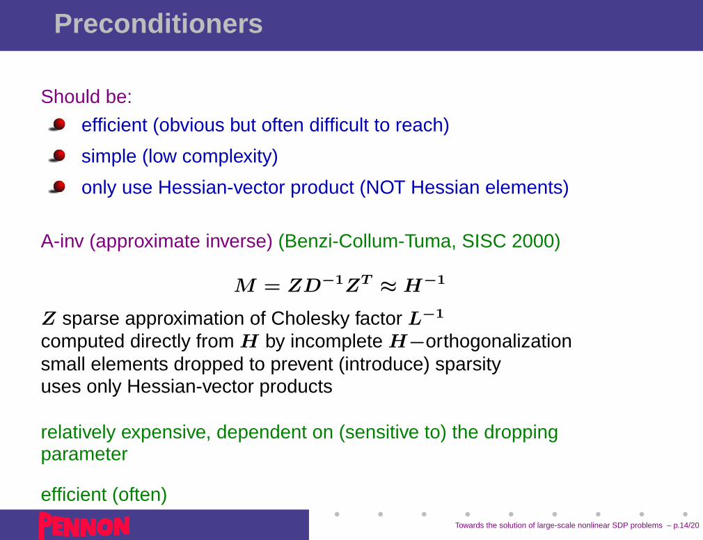
Preconditioners
Should be:
efficient (obvious but often difficult to reach)
simple (low complexity)
only use Hessian-vector product (NOT Hessian elements)
Towards the solution of large-scale nonlinear SDP problems – p.14/20
Preconditioners
Should be:
efficient (obvious but often difficult to reach)
simple (low complexity)
only use Hessian-vector product (NOT Hessian elements)
Diagonal
M = diag (H)
simple, not (considered) very efficient
Towards the solution of large-scale nonlinear SDP problems – p.14/20
Preconditioners
Should be:
efficient (obvious but often difficult to reach)
simple (low complexity)
only use Hessian-vector product (NOT Hessian elements)
Symmetric Gauss-Seidel
M = LT D−1L where H = D − L − LT
relatively efficient, a bit too costly
Towards the solution of large-scale nonlinear SDP problems – p.14/20
Preconditioners
Should be:
efficient (obvious but often difficult to reach)
simple (low complexity)
only use Hessian-vector product (NOT Hessian elements)
L-BFGS (Morales-Nocedal, SIOPT 2000)–start with CG (no precond.)–use CG iterations as correction pairs → build M using L-BFGS–next Newton step → use M as preconditioner–from CG iterations build new M
relatively inexpensive (16–32 correction pairs)
mixed success
Towards the solution of large-scale nonlinear SDP problems – p.14/20
Preconditioners
Should be:
efficient (obvious but often difficult to reach)
simple (low complexity)
only use Hessian-vector product (NOT Hessian elements)