Candidate number: 501601 Word count: 6257 TP19: Models of granular networks in two and three dimensions Supervisor: Dr Mason Porter I develop several new models that attempt to reproduce the structure of two-dimensional granular materials, and compare them with experiment using diagnostics from network science. I discuss one model that treats granular networks as a perturbation of a close-packed hexagonal lattice, and two models that are modifications of the random geometric graph (RGG). One of these modified RGGs simulates the forces that compressed particles exert on each other and displaces them accordingly. This model is found to be a good model of granular materials, in that its network properties appear to be very close to those of real granular networks; however, its effectiveness does not seem to depend upon the form of the force law implemented. I then briefly examine the three-dimensional analogues of two of the models. 1 Introduction 1.1 Granular materials A granular material consists of a large number of macroscopic particles (for example, grains of sand) [1]. Understanding flows of granular materials is im- portant in predicting geophysical hazards [2], as is understanding the nature of the jamming transition that occurs when a granular material becomes rigid under increasing pressure [3]. Further important yet poorly understood phenomena are the propagation of sound and the distribution of forces in granular packings. It has been proposed that the appearance of force chains may be a barrier to our understand- ing in this area [4]. The phrase ‘force chain’ refers to the observation that stresses in granular materials are transmitted through the system along chains of par- ticles [5]. These distinctive chains only include a frac- tion of all the particles, and they snake through the material in an inhomogeneous and seemingly unpre- dictable manner (see Fig. 1). In [6], the structure of force chains was approached from a network-science perspective. It was found that the mean force on a particle is significantly correlated with its intracom- munity strength z -score, which is a measure of the particle’s connectivity within its local network com- munity (see Sections 1.2 and 1.5 for descriptions of network connectivity and communities). The results in [6] indicate that a network-science perspective can provide powerful tools with which to probe the struc- ture of granular materials. Motivated by this, I use diagnostics from network science as a means to as- sess the effectiveness of different models of granular materials. This report is organised as follows. In the remain- der of this section, I briefly describe some relevant concepts from network science and describe the ori- gin of the experimental data that I will be comparing the models to. In Section 2, I describe each model in detail and explain its motivation. I also discuss each model’s performance when compared with experi- ment using network diagnostics. In Section 3, I anal- yse the force-modified RGG model in more detail, comparing the distribution of forces and compres- sions that it predicts with results from experiment, and in Section 4 I investigate how the effectiveness Figure 1: Force chains observed in a granular medium con- sisting of photoelastic disks, which emit light when com- pressed [7]. See Section 1.4. Image credit to Eli Owens and Karen Daniels (used with permission). 1
Transcript
Candidate number: 501601Word count: 6257
TP19: Models of granular networks in two and three dimensions
Supervisor: Dr Mason Porter
I develop several new models that attempt to reproduce the structure of two-dimensional granular materials,and compare them with experiment using diagnostics from network science. I discuss one model that treatsgranular networks as a perturbation of a close-packed hexagonal lattice, and two models that are modificationsof the random geometric graph (RGG). One of these modified RGGs simulates the forces that compressedparticles exert on each other and displaces them accordingly. This model is found to be a good model ofgranular materials, in that its network properties appear to be very close to those of real granular networks;however, its effectiveness does not seem to depend upon the form of the force law implemented. I then brieflyexamine the three-dimensional analogues of two of the models.
1 Introduction
1.1 Granular materials
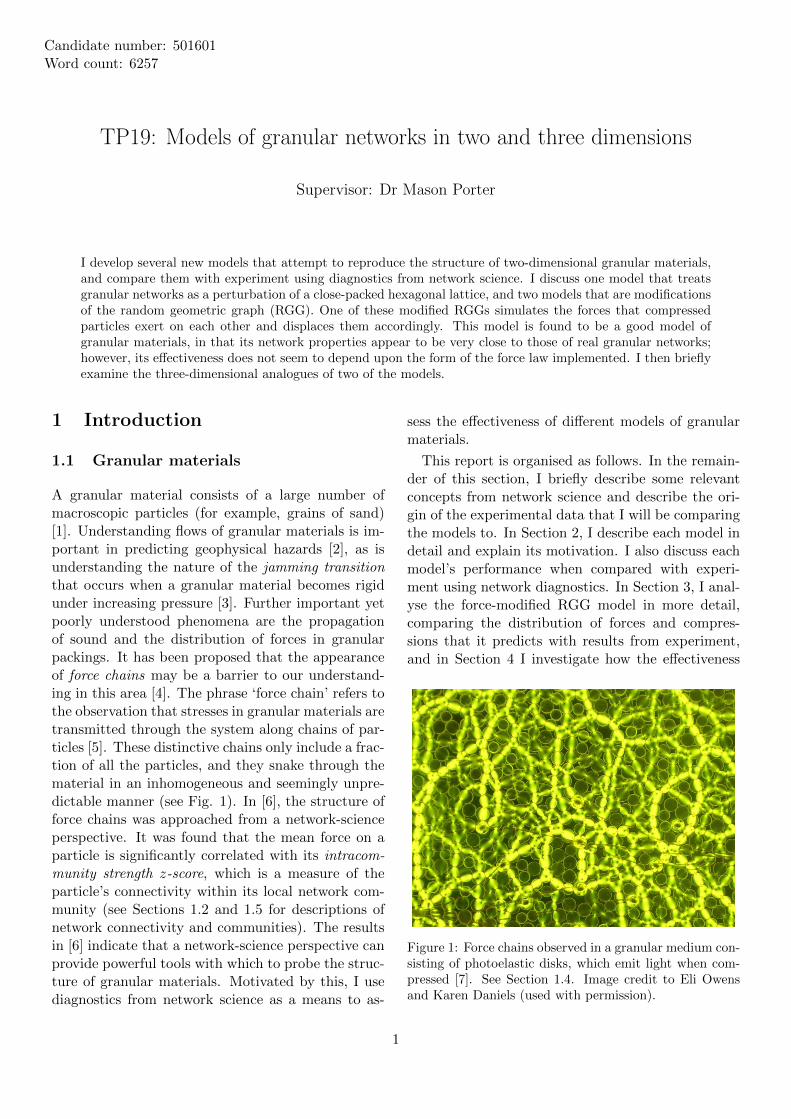
A granular material consists of a large number ofmacroscopic particles (for example, grains of sand)[1]. Understanding flows of granular materials is im-portant in predicting geophysical hazards [2], as isunderstanding the nature of the jamming transitionthat occurs when a granular material becomes rigidunder increasing pressure [3]. Further important yetpoorly understood phenomena are the propagationof sound and the distribution of forces in granularpackings. It has been proposed that the appearanceof force chains may be a barrier to our understand-ing in this area [4]. The phrase ‘force chain’ refers tothe observation that stresses in granular materials aretransmitted through the system along chains of par-ticles [5]. These distinctive chains only include a frac-tion of all the particles, and they snake through thematerial in an inhomogeneous and seemingly unpre-dictable manner (see Fig. 1). In [6], the structure offorce chains was approached from a network-scienceperspective. It was found that the mean force on aparticle is significantly correlated with its intracom-munity strength z-score, which is a measure of theparticle’s connectivity within its local network com-munity (see Sections 1.2 and 1.5 for descriptions ofnetwork connectivity and communities). The resultsin [6] indicate that a network-science perspective canprovide powerful tools with which to probe the struc-ture of granular materials. Motivated by this, I usediagnostics from network science as a means to as-
sess the effectiveness of different models of granularmaterials.
This report is organised as follows. In the remain-der of this section, I briefly describe some relevantconcepts from network science and describe the ori-gin of the experimental data that I will be comparingthe models to. In Section 2, I describe each model indetail and explain its motivation. I also discuss eachmodel’s performance when compared with experi-ment using network diagnostics. In Section 3, I anal-yse the force-modified RGG model in more detail,comparing the distribution of forces and compres-sions that it predicts with results from experiment,and in Section 4 I investigate how the effectiveness
Figure 1: Force chains observed in a granular medium con-sisting of photoelastic disks, which emit light when com-pressed [7]. See Section 1.4. Image credit to Eli Owensand Karen Daniels (used with permission).
1
of this model is dependent on the precise form of theforce law it implements. In Section 5, I extend two ofthe models to three dimensions and compare the re-sults to the two-dimensional case. Finally, in Section6, I discuss my findings and conclusions.
1.2 Spatial networks
A network is a set of nodes and an associated set ofedges that define pairwise connections between thenodes. For a network with N nodes, we label thenodes i = 1, 2, 3, . . . , N and label edges using the un-ordered pair of integers (i, j), which then representsan undirected connection between nodes i and j1.
A spatial network is a network whose nodes areembedded in some space possessing a metric [8]. Agranular material can be used to define a networkembedded in a 2D Euclidean plane, with particlesrepresented by nodes that are connected by an edgeif and only if the particles are in contact. This rep-resentation is a particularly natural one, so it seemsreasonable to expect a network-science perspective toprovide enlightening ways of analysing the structureof granular materials.
It is important to clarify what is meant when twoparticles are said to be “in contact”. If two particleshave positions xi and xj and respective radii ri and rjwhen uncompressed, we define them to be in contactif and only if |xi − xj | ≤ ri + rj .
1.3 Some definitions
A network with N nodes can be described by its ad-jacency matrix [9], an N ×N matrix whose elementstake the values
Aij =
{1, if i and j are connected,
0, otherwise.(1)
A weighted network has a weight wij associated withthe edge (i, j) that connects nodes i and j. Theseweights might come from the physical distance be-tween two connected nodes, or can be the force thattwo particles exert on one another. For a weightednetwork, the weighted adjacency matrix is:
Wij =
{wij , if i and j are connected,
0, otherwise.(2)
The adjacency matrix encodes all the informationabout the network and allows direct calculation of
1We can also define a directed network, in which edges arelabelled using an ordered pair of integers (i, j), which representsa directed connection from node i to node j.
many useful quantities. For example, the degree kiof node i is the number of nodes to which it is con-nected. In terms of the adjacency matrix,
ki =∑j
Aij . (3)
A path from node i to node j is a sequence of edgesthat connect a sequence of nodes starting at node iand terminating at node j. The length of the pathis the number of edges in the path (or for weightednetworks the sum of the weights of those edges). Ageodesic path is a path between two nodes with theshortest possible length. Geodesic paths between twonodes are in general not unique.
A planar network is a network whose nodes can beplaced in the plane in such a way that the edges donot intersect each other (except at the nodes).
1.4 Experimental data
Owens and Daniels [7] performed experiments on aset of bidisperse 2D granular packings. A bidispersemedium contains particles of two different sizes, whilea monodisperse medium contains particles of identi-cal size. A collection of disks were cut from VishayPSM-4 photoelastic material, with thickness 6.35 mmand radii r1 = 4.5 mm and r2 = 5.5 mm. Approx-imately 1000 particles were packed into a containerwith an open top, so that they were confined onlyby gravity. The average packing fraction of these ar-rangements was 0.84± 0.01, where the packing frac-tion is defined as the fraction of the total area occu-pied by the particles. In total 17 different arrange-ments were studied, each of which was obtained bymanually rearranging the disks. The photoelasticityof the particles means that the contact forces can beestimated by comparing photographs of the systemto calibration images for known forces [6]. Data wasthereby obtained for both the contact networks andthe weighted force networks.
1.5 Network diagnostics
In network science, many diagnostics have been in-troduced as means of quantifying the properties ofnetworks [9]. The beauty of applying network scienceto granular materials is that even though these diag-nostics were not introduced with granular networksin mind, they can give insightful information aboutthe structure of the network and hence the structureof the material.
2
Network diagnostics can be defined for bothweighted and unweighted networks. In my analyses,I compare only diagnostics of the unweighted contactnetworks. Below I list the diagnostics that I used.Diagnostics (with the exception of communicabilityand mean shortest distance) were calculated usingcode from the Brain Connectivity Toolbox [10]. See[6, 9] for precise definitions.
� Node (edge) betweenness centrality. Node (edge)betweenness centrality of a given node (edge)measures the number of geodesic paths thatpass through that node (edge). This diagnosticgives an indication of a node’s (or edge’s) impor-tance within a network — for example, a stationin a rail network has a high node betweennesscentrality if a large number of rail routes passthrough it.
� Clustering coefficient and transitivity. These twodiagnostics are closely related, and give infor-mation about local clustering within a network.A node with a high clustering coefficient has ahigh number of connections between its neigh-bours. Transitivity is the proportion of con-nected triplets of nodes that also form triangles.
� Assortativity. This quantifies the extent towhich the degrees of connected nodes are cor-related.
� Global and local efficiency. Global efficiencyquantifies how well a signal transmits througha network, whereas the local efficiency of a nodequantifies how well a signal transmits within alocal subgraph that includes that node.
� Mean shortest distance. This is simply the meanlength of the geodesic paths in a network.
� Maximised modularity. Modularity is relatedto the problem of community detection. Theaim of community detection is to partition anetwork into non-overlapping communities suchthat the edge density within communities is largewhereas connections between communities aresparse. Community detection algorithms max-imise a quantity known as modularity — themaximised value then gives a measure of howwell the network can be partitioned into com-munities2.
2I use the Louvain algorithm [11] to optimise the modular-ity.
� Subgraph centrality. This diagnostic quantifiesthe extent to which a given node participates inthe subgraphs of a network.
� Communicability. The communicability of a pairof nodes attempts to describe the ease of commu-nication between the nodes by counting the num-ber of paths between them while down-weightingthe contributions from longer paths.
In addition to these diagnostics, I also developed twonew measures in the course of my investigations:
� tr(eA − I). This quantity is closely related tocommunicability except that rather than count-ing paths between different nodes, it counts loopsthat start and end at the same node.
� Path-weighted betweenness. This diagnostic isidentical to node betweenness centrality exceptthat it down-weights the contribution from eachpath by a factor 1/l!, where l is the length of thepath.
For diagnostics that give a value for each individualnode (or edge), I calculate the mean over all the nodes(or edges) to provide a single number to characterisethe whole network.
2 Models
2D granular networks are highly constrained by somebasic physical principles:
� They are embedded in 2D, so they must be pla-nar;
� The compression between two particles in con-tact with one another is generally small com-pared to the radii of the particles, so there is alimit to how close any two nodes can be;
� There is a geometrical restriction on the max-imum degree of each node: for monodispersedisks — or bidisperse disks whose radii (r2 > r1)are in the ratio r2
r1< 1.3 — no particle can be in
contact with any more than six other particles3.
3Let r1 and r2 be such that n circles with radius r1 can bepacked around a circle with radius r2. Then the centres of twoadjacent smaller circles subtend an angle θ = 2arcsin r1
r1+r2at
the centre of the larger circle (by simple trigonometry). Hencer2r1
= cosecπn− 1. In this case n = 7, so r2
r1≈ 1.3.
3
Figure 2: From left to right, sections of packings generated by the bidisperse RGG, the p(ρ)-modified RGG, and theforce-modified RGG.
I develop different models to focus on each of theseconstraints. In the following subsections, I present adescription of each model and a brief examination ofits performance. I give the network diagnostics foreach model along with experimental data in Table 1in Appendix B.
2.1 Random geometric graph
A very crude model is the random geometric graph(RGG) in 2D. Here we place N particles uniformly atrandom within a rectangular subset of R2 (whose di-mensions approximately match the dimensions of theexperimental setup) and connect them by an edge ifthey are separated by a distance of less than 2R. Wechoose R so that the edge density (the ratio of thenumber of edges to the number of nodes) of the re-sulting network matches the experimental data. Notethat these RGGs will in general not be planar net-works. Therefore, the only constraint captured bythe RGGs is the dimensionality of the space in whichthe network is physically embedded, because we usethe 2D Euclidean metric to define distance betweennodes. This model has already been studied in thecontext of granular networks in [6], where the RGG isused as a null-model network with which to comparenetwork diagnostics computed from the experimentaldata.
We can also crudely model a bidisperse system byassigning each particle a radius ri that can take oneof two values. We then connect two particles by anedge if the distance between them is dij < R(ri+ rj),where again R is a parameter that we can change to
match the edge density with experiment.
The RGG is a poor model of granular networks.As has already been noted in [6], the network diag-nostics are significantly different for an ensemble ofRGGs versus the experimental networks (see Table 1in Appendix B). We find that RGGs are locally moreconnected, with higher values of clustering coefficientand local efficiency than we find in the experimentaldata. This makes sense, since we have not imposedany constraint on the maximum degree of a node, andthe non-planarity of the RGGs allows connections be-tween particles that are physically impossible in areal granular network. Interestingly, the bidisperseversion of the RGG fared no better in matching theexperimental data than the monodisperse version.
However, the RGG results are useful because theygive a baseline against which to compare the resultsfrom the other models. Comparing any diagnosticagainst its value for the RGGs allows us to get asense of what order of magnitude to expect, and whatconstitutes a close agreement (or otherwise) with ex-periment. We will see that all of the other modelsperform significantly better than the RGGs. This isto be expected, because each of the models imposesconstraints that are motivated by real effects in gran-ular materials.
2.2 p(ρ)-modified RGG
There are many ways to modify the RGG model tomore accurately reflect the structure of granular ma-terials. One of the most evidently unphysical aspectsof the simple RGG model is that two particles can
4
be arbitrarily close to one another. Particles exert arepulsive force when compressed, so there is a limitto how close we expect to find particles to each other,for a given packing fraction.
Define the proximity ρ, given an arrangement ofpre-placed particles, as the distance from a givenpoint to the nearest particle. Proximity is thus afunction of position in the plane. We can then mod-ify the RGG model by placing particles one by one —a point is chosen uniformly at random and a particleis placed there with a probability p(ρ) — a function ofthe point’s proximity. If p→ 0 for small proximities,then the resulting arrangement has a constraint onhow close particles can be positioned to one another.
A simple choice for the function p(ρ) is
p(ρ) =
{0, for ρ < 2αri,
1, for ρ ≥ 2αri,(4)
where ri is the radius of the particle being placed.The value of α puts a limit on the number of particlesof a given radius that can be placed in a given area. Iplaced bidisperse particles into a rectangular region,matching the dimensions and the sizes of the particlesto experiment. Given this setup, the highest value ofα that allowed the appropriate number of particlesto be placed was α ≈ 0.8. It is reasonable to usethe highest value of α (< 1) as possible, because, asI have already noted, compressions between particlesare generally small compared to their radii and so weshould enforce as strict a constraint as possible onhow close particles can be to one another.
Particles are then connected using a similar proce-dure to that used for the simple RGG model. Figure 2shows particle arrangements generated from the sim-ple RGG, the modified RGG, and the force-modifiedRGG (see Section 2.4). As might be expected sim-ply from a visual comparison of these models, thep(ρ)-modified RGG performs much better than theoriginal RGG in almost every diagnostic (see Table 1in Appendix B).
2.3 Modified lattice
A very important property of 2D packings of disksis their tendency to crystallise into lattice-like struc-tures [12]. Under high enough pressures, a monodis-perse packing can crystallise into a hexagonal lattice,which is the optimal packing arrangement for circlesin 2D. Crystallised packings do not exhibit the forcechain structure that we observe in irregular packings.This is the main reason that Owens and Daniels used
bidisperse particles — particles with different radiiare much less likely to crystallise into regular struc-tures.
Nevertheless, there is a definite tendency for bidis-perse packings to locally approximate hexagonalpackings. From visual inspection, we see that 2Dpackings include some regions that are reminiscentof hexagonal lattices (See Fig. 3). This motivatesa modified lattice model, which treats granular net-works as a perturbation of a hexagonal lattice. Start-ing with the contact network for a rectangular section(dimensions to match experiment) of a perfect close-packed lattice, I remove edges uniformly at randomuntil the edge density matches experiment.
Figure 3: On a small scale, bidisperse particles can stillpack into a regular hexagonal structure. Original imagefrom Owens and Daniels [7] (used with permission).
Note that all the other models give a set of particlepositions as their output. This set contains enoughinformation to construct the contact network (onceR is fixed). The modified lattice model is differentin that it directly outputs the contact network. Thisnetwork does not contain enough information to re-construct a set of particle positions. This means that,while the other models can be visualised by plottingthe positions of the particles (as in Fig. 2) the mod-ified lattice model is not amenable to a visual repre-sentation. It is a model only of the contact network,and makes no attempt to model the precise physicalarrangement of particles.
Despite this, the network diagnostics of this modelmatch very well to those of the experimental data(see Table 1). The match is particularly good fordiagnostics which characterise global, system scaleproperties of the network — specifically, node andedge betweenness centrality, mean shortest distance,
5
and global efficiency.
2.4 Force-modified RGG
An obvious constraint on granular materials is thatthey are formed of particles that obey physical laws.In particular, the particles are acted on by gravity(unless the plane is horizontal) and by forces fromthe other particles and the walls of the container.In Hertzian contact theory, the force between twocompressed particles takes the form
f ∝ δβ, (5)
[7] where δ is the total compression and β is an expo-nent which depends on the geometry of the particles.For the particles in the experimental data I used, theexponent β was found to be approximately 5/4 [7].
I modify the crude RGG model by calculating theinter-particle forces using force law (5) for a randomarrangement of particles. I then allow each particleto move a displacement di = εfi, where fi is the totalforce on particle i, and ε is a resolution parameter. Ithen recalculate the forces, and repeat the process.
There are subtleties involved in choosing an appro-priate value for the parameter ε. Ideally ε would betaken to be arbitrarily small4 so that the system couldmove smoothly and incrementally into its equilibriumarrangement. However, reducing ε dramatically in-creases the computation time.
A larger value of ε is useful at the beginning of thesimulation, because the particles start out clusteredtogether and need to move significant distances in or-der to fill the spaces in between. However, this missesthe fine detail needed to home in on the equilibriumarrangement, and the particles end up hopping backand forth around their equilibrium position withoutever getting there.
To address this issue, I monitor the potential en-ergy of the system. Since the model is supposed toallow the particles to relax under the forces they exerton one another, the potential energy should decreasewith every step of the simulation. The code was mod-ified so that if after any step the potential energybecomes higher than it was after the previous step,the resolution parameter is tuned down by a constantfactor. This allows me to start the simulations witha relatively high value of ε, which is then modified asthe simulation progresses so that the system is alwayssensitive at the appropriate distance scales. The po-tential energy will eventually tend to an asymptotic
4Here, ‘small’ means that the mean distance moved by eachparticle is small compared to the dimensions of the container.
value, and there will come a point at which small ad-justments in particle positions are unimportant. Onemethod I use to determine the moment at which thisoccurs is to calculate the adjacency matrix at everystep. If the adjacency matrix remains the same for asignificant number of iterations, I judge it appropri-ate to end the simulation. See Fig. 2 for a particlearrangement generated using this model. For moredetails on the implementation of the model, see Ap-pendix A.
This model is the most sophisticated one that Iinvestigated, and is the closest to real-world granu-lar networks because it includes more physical con-straints than the other models. Therefore, we expectit to perform particularly well under our network di-agnostics. This is indeed what we find, especiallycompared with the simple RGG and p(ρ)-modifiedRGG models. The diagnostics for which the force-modified RGG performs best appear to be ones thatare especially sensitive to local structure — cluster-ing coefficient, local efficiency, modularity, subgraphcentrality, transitivity, communicability, tr(eA − I),and path-weighted betweenness (Table 1). The mod-ified lattice model still seems to better capture theglobal properties of the networks.
For the diagnostics that are more sensitive to globalproperties, the force-modified RGG is actually notmuch better than the p(ρ)-modified RGG model. Itis interesting that the improvement from the cruder
Figure 4: Force chains in the force-modified RGG model.Thickness of the lines indicates the strength of the inter-particle forces.
6
model to the more sophisticated one does not showup significantly in the global network diagnostics.The conclusion is striking: modelling the forces be-tween particles causes a significant improvement inthe model’s local structure, but seems to have littleeffect on the global structure.
3 Physical analysis of the force-modified RGG
Thus far, I have focussed on using network diagnos-tics to assess the effectiveness of the models. Sincethe force-modified RGG model incorporates a forcelaw, it makes sense to analyse this model from aphysics perspective as well.
Figure 4 is a plot of the force chains for a parti-cle arrangement generated by this model. I calcu-late the forces between particles using force law (5),with β = 5/4. Encouragingly, the force-modified RGGmodel reproduces force chains that are reminiscent ofexperiment (see Fig. 1).
To investigate these matters more quantitatively,I also examine the force distributions. In Fig. 5, Iplot the force distribution as measured in experiment,compared to the force distribution for force-modifiedRGG packings generated at the same packing frac-tion. Note the presence of more than one peak inthe experimental distribution. The force distribu-tion generated by the force-modified RGG has onlyone distinct peak, so some aspect of the physics hasclearly been overlooked by this model. To understandwhat the model is missing, we return to the force law(5). Including the constant of proportionality, wewrite it as
fij = αδβij , (6)
where we recall that δij is the total compression be-tween particles i and j. In Hertzian contact theory,the constant α is generally a function of the particles’geometry. In the force-modified RGG model, the par-ticles are displaced in increments proportional to theresolution parameter ε, so the constant α is unnec-essary if we assume it takes the same value for allparticles. I therefore did not incorporate it into theforce-modified RGG model. However, we would ac-tually expect α to be a function of the radii of thetwo particles. Therefore,
fij = α(ri, rj)δβij . (7)
To generate a physically more realistic force distribu-tion, we need to determine the three values: α(r1, r1),
Figure 5: Normalised force distributions for experiment(averaged over 17 different packings) and the force-modified RGG (averaged over 20 realisations). The dis-tribution from the model is scaled so that the mean forcematches experiment.
α(r1, r2), and α(r2, r2), where r1 and r2 are the twodifferent radii of the bidisperse particles. We then ob-tain a force distribution that is a sum of three (single-peak) distributions, with one peak for each distinctvalue of α. This may be the mechanism behind themore complex force distribution that we observe inexperiment.
In an attempt to improve the force-modified RGGmodel, one can try to determine the values of α byfitting to experiment. Indeed, including as much ofthe known physics as possible seems an obvious wayof improving the model. However, as I shall discussin Section 4, the precise force law used in the genera-tive stage seems to have little effect on the model’s ef-fectiveness, particularly its effectiveness at modellingnetwork properties.
Another relevant distribution is the distribution ofcompressions (i.e. the values of δij in the above equa-tions). The δ-distribution is simpler in that it doesnot depend on the different values of α, so we canuse it instead of the force distribution as a means ofcomparing the model to experiment.
In Fig. 6, we compare the δ-distributions from ex-periment and from the force-modified RGG. I usedsets of packings which were generated at the samepacking fraction as the experiments. Interestingly,the peak of the experimental distribution is at asignificantly higher compression. For non-identical
7
Figure 6: Normalised δ-distributions for the force-modifiedRGG (averaged over 20 realisations) compared to exper-iment (averaged over 17 different packings), at the samepacking fraction. I give values of δ in units of 〈r〉, themean particle radius.
packing fractions, we might expect to find a higherpeak compression in one than the other. However,since both are at the same packing fraction, this isan undesirable result. A lower peak compression sug-gests that the force-modified RGG model generatespackings with too low a potential energy.
To investigate further, I calculate the mean poten-tial energy of the packings generated by the force-modified RGG model and compare to experiment.The potential energy in both cases can be calculatedfrom the particles’ positions. In this calculation I as-sume all values of α to be the same and equal to 1, sothe values are not strictly accurate and are useful onlyfor comparison5. I obtain the mean value 8.88×10⁻⁶
(with a standard deviation of 0.99 × 10⁻⁶) for theexperimental packings and 1.74× 10⁻⁶ (standard de-viation 0.47×10⁻⁶) for the force-modified RGG pack-ings.
4 Sensitivity to the force law
We have found that including a model of the forcesbetween particles significantly improves the RGG’seffectiveness at describing granular network structure
5The explicit expression I use to calculate the potential be-tween particles i and j is Vij = δβ+1
ij . This is strictly onlyproportional to the potential, but since I use it only for com-parison, this technicality is unimportant.
(especially locally). It is important to ask whetherthe model’s effectiveness relies on using the correctforce law. As we saw in Section 3, the force lawcould have been made more realistic by choosing cor-rect values for the coefficients α(ri, rj), instead of as-suming that they were all equal. Would the modelperform better with such an improvement?
To investigate how sensitive the network propertiesof the model are to the force law, I generated particlearrangements for different values of the parameter β.As I have mentioned, for the particles used in theexperiments, β ≈ 5/4. In Table 2 in Appendix B, Ishow the results for the various network diagnosticsfor β = 5/4 and β = 0. The latter is an extremecase, in which the force between a pair of particlesis independent of their compression and particles allexert the same force on one another if they are incontact.
Interestingly, the results for the two cases arenearly identical. All differences are well within onestandard deviation. In the force-modified RGG wemight as well have used a force law that is simplerboth analytically and computationally, as it wouldstill generate networks that are good models of realgranular networks (in so far as the chosen diagnosticscan reveal).
This suggests that the important constraint ongranular networks is not the exact form of the forcelaw between particles but rather the fact that theyexert some force on each other. The network proper-ties that I studied do not seem to be sensitive to theforces between particles — however, it is importantthat some repulsive force is modelled.
5 Extension to 3D
The simplicity of the models that I have developed al-lows a straightforward extension to three-dimensionalgranular materials. Without experimental data in3D, the best we can do is to compare the results fromthe models. In Table 3 in Appendix B, I present thenetwork diagnostics for the force-modified RGG ver-sus the modified lattice model. I also give resultsfrom a 3D version of the simple RGG for compari-son. I use the same number of particles in each modeland match the edge density as before. For the force-modified RGG and simple RGG, I use a containerwhose sides are all of equal length; for the modifiedlattice, I start with an approximately cubic sectionof a 3D hexagonal close-packed lattice.
We no longer observe the particularly good agree-
8
ment between the force-modified RGG and modifiedlattice that we saw in 2D. This is especially true of themore local diagnostics, such as clustering coefficientand local efficiency, for which the disparity betweenthe two models has significantly increased.
The force-modified RGG imposes the most realisticphysical constraints — this suggests that the resultsfrom this model will be the most reliable and in bestagreement with real 3D granular materials. Exper-imental data is necessary to further investigate thispossibility.
6 Discussion and conclusions
I have investigated three novel models of granularnetworks. The main analysis I performed on thesemodels was a comparison of network diagnostics forthe unweighted contact networks. The most sophisti-cated of these models, the force-modified RGG, pro-vides a model not only of the contact network butalso of the weighted force network. I compared thismodel’s prediction for the distributions of forces andcompressions to experiment. Then I extended theforce-modified RGG and the modified lattice mod-els to three dimensions and repeated the analysis oftheir network diagnostics, comparing their behaviourin 3D and 2D.
The network analysis of the RGG-based modelswas interesting because it illustrated how includingmore physical constraints in a model improved itsperformance in comparison to experiment. The sim-ple RGG model included no constraints other thanthe fact that it embedded the network in a two-dimensional space. The p(ρ)-modified RGG modelattempted to crudely model the constraint that parti-cle compressions are small compared to their radii bypreventing particles from being closer than 0.8 timesthe sum of their radii. Finally, the force-modifiedRGG model attempted to simulate the actual forcesbetween particles. The performance of the modelsimproved with each constraint — the simple RGGperformed worst, followed by the p(ρ)-modified RGG,while the force-modified RGG was the closest matchto experiment (see Table 1).
An enlightening distinction that a network analy-sis allows us to make is the distinction between localand global properties of the system. Each networkdiagnostic is sensitive at a characteristic size scale.For example, betweenness centrality is related to thenumber of geodesic paths that go through a givennode/edge, so its value depends on the structure of
the rest of the network. In this sense its value foreach node/edge is sensitive to global properties of thenetwork. The main reason I introduced path-weightedbetweenness was to create a related measure that wasmore sensitive to local properties. As described inSection 1.5, the contribution of each path to this di-agnostic is down-weighted by a factor 1/l!, where lis the length of the path. Consequently, this diag-nostic is much less sensitive to large-scale structure,and the leading contribution comes from short pathsin the vicinity of each node. A related diagnostic istr(eA − I), which counts the number of loops thatstart and end at a given node, and in a similar waydown-weights the contributions from longer loops.
As was discussed in Section 2, the improvementfrom the p(ρ)-modified RGG to the force-modifiedRGG mainly shows up in the diagnostics which aresensitive to local structure. As far as the global di-agnostics are concerned, the force-modified RGG isonly a slight improvement on the p(ρ)-modified RGG.The natural conclusion to draw is that modelling indetail the forces between particles significantly im-proves the local structure of a model, while accurateglobal properties can be modelled by much simplerconstraints, like the one the p(ρ)-modified RGG isbased upon. Since it is always desirable to have amodel that gives accurate predictions with minimalphysical constraints, it is valuable to be able to iden-tify which constraints different properties of granularnetworks depend on.
An especially interesting result was found duringthe investigations described in Section 4. Althoughmodelling the forces between particles improves thelocal structure of the RGG model, none of the diag-nostics I used appear to be affected by the preciseform of the force law. Whether or not there are anydiagnostics of the unweighted network that are sen-sitive to the choice of force law is a question thatfurther investigations might shed light on.
The physical analysis of the force-modified RGG inSection 3 brought to light one issue with this model.It generates packings which appear have a lower po-tential energy than the packings studied in experi-ment. One method of overcoming this problem mightbe to stop the simulation when the potential energyreaches a certain value. This would introduce anextra parameter to the model, but might generatepackings which more closely resemble real granularmaterials. Repeating both the network and physi-cal analyses of Sections 2 and 3 could support thissuggestion.
To conclude, diagnostics from network science have
9
made it possible to perform a much more detailedanalysis of granular materials — and models thereof— than a purely physical approach would have al-lowed. I have been able to examine the effectivenessof different models at different size scales, using a setof diagnostics that are sensitive to a wide range of sys-tem properties. The diagnostics I have used are, how-ever, far from a complete set, and more work couldbe done examining how granular networks and theirmodels perform under different network diagnostics.
As discussed in Section 2, the modified latticemodel has network diagnostics that match verywell to experiment (especially on global properties).Whether or not there are network diagnostics forwhich the modified lattice shows up as a poor modelis a question that might be answered by further in-vestigation. The modified lattice does not attempt tomodel the physics of granular networks to the extentthat the force-modified RGG does, and perhaps thisis showing up in the fact that the force-modified RGGoutperforms the modified lattice on local diagnostics(in particular communicability and tr(eA−I)). Theremay however be other diagnostics for which this de-ficiency shows up more significantly.
Network diagnostics appear to be useful and highlysensitive tools for understanding the structure ofgranular materials. Further work might uncover moreappropriate network diagnostics for application tothis area, as well as lead to a better understanding oftheir dependence on the physical properties of gran-ular materials.
Acknowledgements
I would like to thank Karen Daniels for providing ex-perimental data and insightful comments, and LisaManning for providing MATLAB code and data fromsimulations. I would especially like to thank my su-pervisor Mason Porter for many useful comments andinvaluable discussions.
References
[1] K. Hutter and K. R. Rajagopal. On flows of gran-ular materials. Continuum Mech. Thermodyn. 6819 (1994).
[2] P. Jop, Y. Forterre, and O. Pouliquen. A consti-tutive law for dense granular flows. Nature Lett.441 727 (2006).
[3] M. van Hecke. Jamming of soft particles: geome-try, mechanics, scaling and isostaticity. J. Phys.:Condens. Matter 22 033101 (2010).
[4] H. A. Makse, N. Gland, D. L. Johnson, and L.M. Schwartz. Why Effective Medium Theory Failsin Granular Materials. Phys. Rev. Lett. 83 5070(1999).
[5] D. M. Mueth, H. M. Jaeger, and S. R. Nagel.Force Distribution in a Granular Medium. Phys.Rev. E 57 3164 (1998).
[6] D. S. Bassett, E. T. Owens, K. E. Daniels, and M.A. Porter. Influence of network topology on soundpropagation in granular materials. Phys. Rev. E86 041306 (2012).
[7] E. T. Owens and K. E. Daniels. Sound propaga-tion and force chains in granular materials. Eu-rophys. Lett. 94 54005 (2011).
[8] M. Barthelemy. Spatial Networks. Physics Re-ports 499 1 (2011).
[9] M. E. J. Newman. Networks: An Introduction.(Oxford University Press, Oxford, 2010).
[10] M. Rubinov and O. Sporns. Complex networkmeasures of brain connectivity: Uses and inter-pretations. NeuroImage 52, 1059 (2009).
[11] V. D. Blondel, J. L. Guillaume, R. Lambiotte,and E. Lefebvre. Fast unfolding of communitiesin large networks. J. Stat. Mech. (2008) P10008
[12] A. Donev, S. Torquato, F. H. Stillinger, andR. Connelly. Jamming in Hard Sphere and DiskPackings. J. Appl. Phys. 95 (3) 989 (2004).
Appendices
A Force-modified RGG algorithm
The equation I used for the force acting on particle iis
fi =∑j 6=i
[(1
2(ri + rj)−
1
2|xi − xj |
)β xi − xj|xi − xj |
]+(ri − xi)βx− (ri + xi − Lx)βx
+(ri − yi)βy − (ri + yi − Ly)βy
(8)
where it is understood that the terms raised to thepower β are only to be evaluated if they are positive.
10
In this equation, ri is the radius of the ith particle andxi and yi are its coordinates, being the componentsof the vector xi. Two walls of the container lie alongthe x and y axes, while the other two lie along thelines x = Lx and y = Ly. The unit vectors along thex and y axes are x and y, respectively. The termsin the sum give the forces from other particles, whilethe final four terms are the forces from each of thewalls.
For the realisations analysed in this report, I usedLx = 0.29 and Ly = 0.38. As described in Section2.4, the particles — whose positions are initially dis-tributed uniformly at random — are moved a dis-tance di = εfi in every step of the simulation. Adifferent starting value of ε is appropriate for differ-ent values of β. I found that, for β = 1.25 and β = 0,good starting values are ε = 8 and ε = 0.001 re-spectively. Higher values often caused the potentialenergy of the system to quickly diverge, while lowervalues made the simulation unnecessarily slow. Atevery step of the simulation the potential energy ofthe system was calculated. The formula used for thiswas
V =∑j 6=i
[(1
2(ri + rj)−
1
2|xi − xj |
)β+1]
+(ri − xi)β+1 − (ri + xi − Lx)β+1
+(ri − yi)β+1 − (ri + yi − Ly)β+1.
(9)
Let Vi be the potential of the system after the ith
iteration. If Vi > Vi−1, then we replace ε→ ε′ = 0.9ε.This ensures that the rearrangement of the particlesbecomes more and more precise as the system getscloser to an equilibrium arrangement.
11
B Network diagnostics
Table 1: Network diagnostics for the experimental networks and models. I take means and standard deviations over 17experimental networks and 20 realisations of each of the models.