174
ETSI TR 101 290 V1.3.1 (2014-07) Digital Video Broadcasting (DVB); Measurement guidelines for DVB systems TECHNICAL REPORT

ETSI TR 101 290 V1.3.1 (2014-07)
Digital Video Broadcasting (DVB); Measurement guidelines for DVB systems
TECHNICAL REPORT
ETSI
ETSI TR 101 290 V1.3.1 (2014-07) 2
Reference RTR/JTC-DVB-340
Keywords broadcasting, digital, DVB, TV, video
ETSI
650 Route des Lucioles F-06921 Sophia Antipolis Cedex - FRANCE
Tel.: +33 4 92 94 42 00 Fax: +33 4 93 65 47 16
Siret N° 348 623 562 00017 - NAF 742 C
Association à but non lucratif enregistrée à la Sous-Préfecture de Grasse (06) N° 7803/88
Important notice
The present document can be downloaded from: http://www.etsi.org
The present document may be made available in electronic versions and/or in print. The content of any electronic and/or print versions of the present document shall not be modified without the prior written authorization of ETSI. In case of any
existing or perceived difference in contents between such versions and/or in print, the only prevailing document is the print of the Portable Document Format (PDF) version kept on a specific network drive within ETSI Secretariat.
Users of the present document should be aware that the document may be subject to revision or change of status. Information on the current status of this and other ETSI documents is available at
http://portal.etsi.org/tb/status/status.asp
If you find errors in the present document, please send your comment to one of the following services: http://portal.etsi.org/chaircor/ETSI_support.asp
Copyright Notification
No part may be reproduced or utilized in any form or by any means, electronic or mechanical, including photocopying and microfilm except as authorized by written permission of ETSI.
The content of the PDF version shall not be modified without the written authorization of ETSI. The copyright and the foregoing restriction extend to reproduction in all media.
© European Telecommunications Standards Institute 2014.
© European Broadcasting Union 2014. All rights reserved.
DECTTM, PLUGTESTSTM, UMTSTM and the ETSI logo are Trade Marks of ETSI registered for the benefit of its Members.
3GPPTM and LTE™ are Trade Marks of ETSI registered for the benefit of its Members and of the 3GPP Organizational Partners.
GSM® and the GSM logo are Trade Marks registered and owned by the GSM Association.
ETSI
ETSI TR 101 290 V1.3.1 (2014-07) 3
Contents
Intellectual Property Rights .............................................................................................................................. 10
Foreword ........................................................................................................................................................... 10
Modal verbs terminology .................................................................................................................................. 10
1 Scope ...................................................................................................................................................... 11
2 References .............................................................................................................................................. 11
2.1 Normative references ....................................................................................................................................... 11
2.2 Informative references ...................................................................................................................................... 11
3 Definitions, symbols and abbreviations ................................................................................................. 13
3.1 Definitions ........................................................................................................................................................ 13
3.2 Symbols ............................................................................................................................................................ 13
3.3 Abbreviations ................................................................................................................................................... 14
4 General ................................................................................................................................................... 17
5 Measurement and analysis of the MPEG-2 Transport Stream ............................................................... 19
5.1 General ............................................................................................................................................................. 19
5.2 List of parameters recommended for evaluation .............................................................................................. 19
5.2.1 First priority: necessary for de-codability (basic monitoring) .................................................................... 21
5.2.2 Second priority: recommended for continuous or periodic monitoring ...................................................... 23
5.2.3 Third priority: application dependant monitoring ....................................................................................... 24
5.3 Measurement of MPEG-2 Transport Streams in networks ............................................................................... 29
5.3.1 Introduction................................................................................................................................................. 29
5.3.2 System clock and PCR measurements ........................................................................................................ 29
5.3.2.1 Reference model for system clock and PCR measurements ................................................................. 29
5.3.2.2 Measurement descriptions ..................................................................................................................... 31
5.3.2.3 Program Clock Reference - Frequency Offset PCR_FO ....................................................................... 31
5.3.2.4 Program Clock Reference – Drift Rate PCR_DR ................................................................................. 32
5.3.2.5 Program Clock Reference - Overall Jitter PCR_OJ .............................................................................. 32
5.3.2.6 Program Clock Reference – Accuracy PCR_AC .................................................................................. 32
5.3.3 Bitrate measurement ................................................................................................................................... 32
5.3.3.1 Bitrate measurement algorithm ............................................................................................................. 33
5.3.3.2 Preferred values for Bitrate Measurement ............................................................................................. 34
5.3.3.3 Nomenclature ........................................................................................................................................ 34
5.3.4 Consistency of information check .............................................................................................................. 35
5.3.4.1 Transport_Stream_ID check ................................................................................................................. 35
5.3.5 TS parameters in transmission systems with reduced SI data ..................................................................... 35
5.4 Measurement of availability at MPEG-2 Transport Stream level .................................................................... 36
5.5 Evaluation of service performance by combination of TS related parameters ................................................. 37
5.6 Parameters for CI related applications .............................................................................................................. 37
5.6.1 Latency ....................................................................................................................................................... 38
5.6.2 CI_module_delay_variation ........................................................................................................................ 39
5.6.3 Input_output_TS comparison...................................................................................................................... 39
5.6.4 CI_module_throughput ............................................................................................................................... 39
5.6.5 Valid TS on CI ............................................................................................................................................ 39
6 Common parameters for satellite and cable transmission media ........................................................... 40
6.1 System availability ........................................................................................................................................... 40
6.2 Link availability ............................................................................................................................................... 40
6.3 BER before RS decoder ................................................................................................................................... 41
6.3.1 Out of service .............................................................................................................................................. 41
6.3.2 In service ..................................................................................................................................................... 41
6.4 Error events logging ......................................................................................................................................... 41
6.5 Transmitter symbol clock jitter and accuracy ................................................................................................... 42
6.6 RF/IF signal power ........................................................................................................................................... 42
6.7 Noise power...................................................................................................................................................... 42
ETSI
ETSI TR 101 290 V1.3.1 (2014-07) 4
6.8 Bit error count after RS .................................................................................................................................... 42
6.9 IQ signal analysis ............................................................................................................................................. 43
6.9.1 Introduction................................................................................................................................................. 43
6.9.2 Modulation Error Ratio (MER) .................................................................................................................. 44
6.9.3 System Target Error (STE) (void) .............................................................................................................. 44
6.9.4 Carrier suppression ..................................................................................................................................... 44
6.9.5 Amplitude Imbalance (AI) .......................................................................................................................... 45
6.9.6 Quadrature Error (QE) ................................................................................................................................ 46
6.9.7 Residual Target Error (RTE) ...................................................................................................................... 46
6.9.8 Coherent interferer ...................................................................................................................................... 46
6.9.9 Phase Jitter (PJ) ........................................................................................................................................... 47
6.9.10 Signal-to-Noise Ratio (SNR) ...................................................................................................................... 48
6.10 Interference ....................................................................................................................................................... 48
7 Cable specific measurements ................................................................................................................. 49
7.1 Noise margin .................................................................................................................................................... 49
7.2 Estimated noise margin .................................................................................................................................... 49
7.3 Signal quality margin test ................................................................................................................................. 49
7.4 Equivalent Noise Degradation (END) .............................................................................................................. 50
7.5 BER vs. Eb/N0................................................................................................................................................... 51
7.6 Phase noise of RF carrier .................................................................................................................................. 51
7.7 Amplitude, phase and impulse response of the channel ................................................................................... 51
7.8 Out of band emissions ...................................................................................................................................... 51
8 Satellite specific measurements .............................................................................................................. 52
8.1 BER before Viterbi decoding ........................................................................................................................... 52
8.2 Receive BER vs. Eb/N0 ..................................................................................................................................... 52
8.3 IF spectrum ....................................................................................................................................................... 53
9 Measurements specific for a terrestrial (DVB-T) system ....................................................................... 53
9.1 RF frequency measurements ............................................................................................................................ 55
9.1.1 RF frequency accuracy (Precision) ............................................................................................................. 56
9.1.2 RF channel width (Sampling Frequency Accuracy) ................................................................................... 56
9.1.3 Symbol Length measurement at RF (Guard Interval verification) .............................................................. 57
9.2 Selectivity ......................................................................................................................................................... 57
9.3 AFC capture range............................................................................................................................................ 57
9.4 Phase noise of Local Oscillators (LO) .............................................................................................................. 58
9.5 RF/IF signal power ........................................................................................................................................... 59
9.6 Noise power...................................................................................................................................................... 59
9.7 RF and IF spectrum .......................................................................................................................................... 59
9.8 Receiver sensitivity/ dynamic range for a Gaussian channel............................................................................ 59
9.9 Equivalent Noise Degradation (END) .............................................................................................................. 60
9.9.1 Equivalent Noise Floor (ENF) .................................................................................................................... 60
9.10 Linearity characterization (shoulder attenuation) ............................................................................................. 61
9.11 Power efficiency ............................................................................................................................................... 61
9.12 Coherent interferer ........................................................................................................................................... 61
9.13 BER vs. C/N ratio by variation of transmitter power ....................................................................................... 61
9.14 BER vs. C/N ratio by variation of Gaussian noise power ................................................................................ 62
9.15 BER before Viterbi (inner) decoder ................................................................................................................. 62
9.16 BER before RS (outer) decoder ........................................................................................................................ 62
9.16.1 Out of Service ............................................................................................................................................. 62
9.16.2 In Service .................................................................................................................................................... 63
9.17 BER after RS (outer) decoder (Bit error count) ................................................................................................ 63
9.18 IQ signal analysis ............................................................................................................................................. 63
9.18.1 Introduction................................................................................................................................................. 63
9.18.2 Modulation Error Ratio (MER) .................................................................................................................. 65
9.18.3 System Target Error (STE) (void) .............................................................................................................. 65
9.18.4 Carrier Suppression (CS) ............................................................................................................................ 65
9.18.5 Amplitude Imbalance (AI) .......................................................................................................................... 66
9.18.6 Quadrature Error (QE) ................................................................................................................................ 67
9.18.7 Phase Jitter (PJ) ........................................................................................................................................... 68
9.19 Overall signal delay .......................................................................................................................................... 69
9.20 SFN synchronization ........................................................................................................................................ 70
ETSI
ETSI TR 101 290 V1.3.1 (2014-07) 5
9.20.1 MIP_timing_error ....................................................................................................................................... 70
9.20.2 MIP_structure_error.................................................................................................................................... 71
9.20.3 MIP_presence_error.................................................................................................................................... 71
9.20.4 MIP_pointer_error ...................................................................................................................................... 71
9.20.5 MIP_periodicity_error ................................................................................................................................ 72
9.20.6 MIP_ts_rate_error ....................................................................................................................................... 72
9.21 System Error Performance ............................................................................................................................... 73
10 Recommendations for the measurement of delays in DVB systems ...................................................... 73
11 Measurements for the second generation terrestrial (DVB-T2) system ................................................. 73
11.1 Introduction ...................................................................................................................................................... 73
11.2 Measurements at the DVB-T2 Modulator Interface (T2-MI) ........................................................................... 74
11.2.1 Introduction................................................................................................................................................. 74
11.2.2 Measurements of the syntax of T2 MI packets ........................................................................................... 75
11.2.2.1 T2MI_packet_type_error_1 .................................................................................................................. 75
11.2.2.2 T2MI_packet_type_error_2 .................................................................................................................. 76
11.2.2.3 T2MI_packet_count_error .................................................................................................................... 76
11.2.2.4 T2MI_CRC_error .................................................................................................................................. 76
11.2.2.5 T2MI_payload_error ............................................................................................................................. 76
11.2.2.6 T2MI_plp_num_blocks_error ............................................................................................................... 76
11.2.2.7 T2MI_transmission_order_error ........................................................................................................... 77
11.2.2.8 T2MI_DVB-T2_Timestamp_error ........................................................................................................ 77
11.2.2.9 T2MI_DVB-T2_Timestamp_discontinuity ........................................................................................... 77
11.2.2.10 T2MI_T2_frame_length_error .............................................................................................................. 77
11.2.3 Checks on the T2-MI MIP (Modulator Information Packet) ...................................................................... 77
11.2.3.1 T2MI_MIP_timestamp_error ................................................................................................................ 77
11.2.3.2 T2MI_MIP_individual_addressing_error ............................................................................................. 77
11.2.3.3 T2MI_MIP_continuity_error ................................................................................................................ 78
11.2.3.4 T2MI_MIP_CRC_error ......................................................................................................................... 78
11.2.4 Check on consistency of T2-MI signalling information ............................................................................. 78
11.2.4.1 T2MI_bandwidth_consistency_error .................................................................................................... 78
11.2.4.2 T2MI_DVB-T2_Timestamp_leap_second_error .................................................................................. 78
11.2.5 Measurements at T2-MI transport layer...................................................................................................... 78
11.2.5.1 Encapsulation of T2-MI packets into MPEG-2 TS (ASI) streams ........................................................ 78
11.2.5.1.1 Parameters relevant to transport of T2-MI packets over MPEG-2 TS............................................. 79
11.2.5.1.2 Informative parameters .................................................................................................................... 79
11.2.5.1.3 Integrity parameters ......................................................................................................................... 79
11.2.5.2 Encapsulation of T2-MI packets into IP streams .................................................................................. 80
11.2.5.2.1 Parameters relevant to transport of T2-MI packets over IP ............................................................. 80
11.3 Measurements for DVB-T2 baseline system .................................................................................................... 82
11.3.1 RF measurements ........................................................................................................................................ 85
11.3.1.1 RF frequency accuracy .......................................................................................................................... 85
11.3.1.2 RF occupied bandwidth ......................................................................................................................... 85
11.3.2 Selectivity ................................................................................................................................................... 85
11.3.3 AFC capture range ...................................................................................................................................... 86
11.3.4 Phase noise of Local Oscillators (LO) ........................................................................................................ 86
11.3.5 RF/IF signal power ..................................................................................................................................... 86
11.3.6 MISO Group Power Ratio .......................................................................................................................... 86
11.3.7 Noise power ................................................................................................................................................ 87
11.3.8 RF and IF spectrum..................................................................................................................................... 87
11.3.9 Receiver sensitivity/ dynamic range for a Gaussian channel ...................................................................... 87
11.3.10 Linearity characterization (shoulder attenuation) ....................................................................................... 88
11.3.11 Power efficiency ......................................................................................................................................... 89
11.3.12 PAPR effect ................................................................................................................................................ 90
11.3.13 P1 Symbol Error Rate ................................................................................................................................. 91
11.3.14 BER before LDPC (inner) decoder ............................................................................................................. 91
11.3.15 Number of LDPC iterations ........................................................................................................................ 91
11.3.16 BER before BCH (outer) decoder ............................................................................................................... 91
11.3.17 Baseband Frame Error Rate BBFER .......................................................................................................... 92
11.3.18 Errored Second Ratio ESR ......................................................................................................................... 92
11.3.19 IQ signal analysis ........................................................................................................................................ 92

ETSI
ETSI TR 101 290 V1.3.1 (2014-07) 6
11.3.19.1 Introduction ........................................................................................................................................... 92
11.3.19.2 Modulation Error Ratio (MER) ............................................................................................................. 93
11.3.19.3 Signal to Interference Noise Ratio (SINR) ............................................................................................ 94
11.3.19.4 Carrier Suppression (CS) ...................................................................................................................... 94
11.3.19.5 Carrier Phase (CPh)............................................................................................................................... 94
11.3.19.6 Amplitude Imbalance (AI) .................................................................................................................... 95
11.3.19.7 Quadrature Error (QE) .......................................................................................................................... 96
11.3.20 SFN synchronization................................................................................................................................... 97
11.3.21 L1 signalling error ...................................................................................................................................... 97
11.3.22 RMS Delay-Spread (RMS-DS)................................................................................................................... 97
11.3.23 Maximum Excess Delay (MED) ................................................................................................................. 98
11.3.24 Receiver Buffer Model (RBM) validation test............................................................................................ 98
11.3.25 Relative power level during the non-P1 part of the FEF (RLF_non_P1).................................................... 98
12 Measurements for the second generation cable system (DVB-C2) ........................................................ 98
12.1 Introduction ...................................................................................................................................................... 98
12.2 Measurements for DVB-C2 baseline system .................................................................................................. 100
12.2.1 RF measurements ...................................................................................................................................... 100
12.2.1.1 RF frequency accuracy ........................................................................................................................ 101
12.2.1.2 RF sampling frequency ....................................................................................................................... 101
12.2.2 AFC capture range .................................................................................................................................... 102
12.2.3 Phase noise of Local Oscillators (LO) ...................................................................................................... 102
12.2.4 RF/IF signal power ................................................................................................................................... 102
12.2.5 Noise power .............................................................................................................................................. 103
12.2.6 RF and IF spectrum................................................................................................................................... 103
12.2.7 Receiver sensitivity/ dynamic range for a Gaussian channel .................................................................... 103
12.2.8 Linearity characterization (shoulder attenuation) ..................................................................................... 103
12.2.9 BER before LDPC (inner) decoder ........................................................................................................... 104
12.2.10 Number of LDPC iterations ...................................................................................................................... 104
12.2.11 BER before BCH (outer) decoder ............................................................................................................. 104
12.2.12 Baseband Frame Error Rate BBFER ........................................................................................................ 104
12.2.13 IQ signal analysis ...................................................................................................................................... 105
12.2.13.1 Introduction ......................................................................................................................................... 105
12.2.13.2 Modulation Error Ratio (MER) ........................................................................................................... 106
12.2.13.3 Amplitude Imbalance (AI) .................................................................................................................. 107
12.2.13.4 Quadrature Error (QE) ........................................................................................................................ 108
12.2.14 L1 signalling error .................................................................................................................................... 108
12.2.15 Receiver Buffer Assumptions (RBA) validation test ................................................................................ 108
Annex A: General measurement methods ......................................................................................... 109
A.1 Introduction .......................................................................................................................................... 109
A.2 Null packet definition ........................................................................................................................... 109
A.3 Description of the procedure for "Estimated Noise Margin" by applying statistical analysis on the constellation data .................................................................................................................................. 110
A.4 Set-up for RF phase noise measurements using a spectrum analyser .................................................. 111
A.5 Amplitude, phase and impulse response of the channel ....................................................................... 112
A.6 Out of band emissions .......................................................................................................................... 113
Annex B: Examples for test set-ups for satellite and cable systems ................................................ 114
B.1 System availability ............................................................................................................................... 114
B.2 Link availability ................................................................................................................................... 114
B.3 BER before RS ..................................................................................................................................... 114
B.3.1 Out of service measurement ........................................................................................................................... 115
B.3.2 In service measurement .................................................................................................................................. 115
B.4 Event error logging ............................................................................................................................... 115

ETSI
ETSI TR 101 290 V1.3.1 (2014-07) 7
B.5 Transmitter symbol clock jitter and accuracy ...................................................................................... 116
B.6 RF/IF signal power ............................................................................................................................... 116
B.7 Noise power .......................................................................................................................................... 116
B.7.1 Out of service measurement ........................................................................................................................... 116
B.7.2 In service measurement .................................................................................................................................. 117
B.8 BER after RS ........................................................................................................................................ 117
B.9 I/Q signal analysis ................................................................................................................................ 117
B.10 Service data rate measurement ............................................................................................................. 117
B.11 Noise margin ........................................................................................................................................ 117
B.11.1 Recommended equipment .............................................................................................................................. 118
B.11.2 Remarks and precautions ................................................................................................................................ 119
B.11.3 Measurement procedure ................................................................................................................................. 119
B.12 Equivalent Noise Degradation (END) .................................................................................................. 120
B.13 BER vs. Eb/N0 ..................................................................................................................................... 120
B.14 Equalizer specification ......................................................................................................................... 120
B.15 BER before Viterbi decoding ............................................................................................................... 122
B.16 Receive BER vs. Eb/N0 ....................................................................................................................... 122
B.17 IF spectrum ........................................................................................................................................... 122
Annex C: Measurement parameter definition ................................................................................... 123
C.1 Definition of Vector Error Measures .................................................................................................... 123
C.2 Comparison between MER and EVM .................................................................................................. 123
C.3 Conclusions regarding MER and EVM ................................................................................................ 124
Annex D: Exact values of BER vs. Eb/N0 for DVB-C systems ........................................................ 125
Annex E: Examples for the terrestrial system test set-ups ............................................................... 126
E.1 RF frequency accuracy ......................................................................................................................... 126
E.1.1 Frequency measurements in DVB-T (void) ................................................................................................... 126
E.1.2 Measurement in other cases (void) ................................................................................................................. 126
E.1.3 Calculation of the external pilots frequency when they do not have continual phase. (void) ........................ 126
E.1.4 Measuring the symbol length and verifying the Guard Interval (void) .......................................................... 127
E.1.5 Measuring the occupied bandwidth, and calculation of the frequency spacing and sampling frequency ...... 127
E.2 Selectivity ............................................................................................................................................. 128
E.3 AFC capture range................................................................................................................................ 128
E.4 Phase noise of Local Oscillators (LO).................................................................................................. 128
E.4.1 Practical information on phase noise measurements ...................................................................................... 129
E.5 RF/IF signal power ............................................................................................................................... 130
E.5.1 Procedure 1 (power metre) ............................................................................................................................. 130
E.5.2 Procedure 2 (spectrum analyser) .................................................................................................................... 130
E.6 Noise power .......................................................................................................................................... 130
E.6.1 Procedure 1 ..................................................................................................................................................... 131
E.6.2 Procedure 2 ..................................................................................................................................................... 131
E.6.3 Procedure 3 ..................................................................................................................................................... 131
E.6.4 Measurement of noise with a spectrum analyser ............................................................................................ 131
E.7 RF and IF spectrum .............................................................................................................................. 132
E.8 Receiver sensitivity/dynamic range for a Gaussian channel ................................................................ 132
ETSI
ETSI TR 101 290 V1.3.1 (2014-07) 8
E.9 Equivalent Noise Degradation (END) .................................................................................................. 132
E.9.1 Description of the measurement method for END ......................................................................................... 133
E.9.2 Conversion method between ENF and END .................................................................................................. 134
E.10 Linearity characterization (shoulder attenuation) ................................................................................. 135
E.10.1 Equipment ...................................................................................................................................................... 135
E.10.2 Remarks and precautions ................................................................................................................................ 135
E.10.3 Measurement procedure (example for UHF channel 47) ............................................................................... 136
E.11 Power efficiency ................................................................................................................................... 137
E.12 Coherent interferer ............................................................................................................................... 137
E.13 BER vs. C/N by variation of transmitter power ................................................................................... 137
E.14 BER vs. C/N by variation of Gaussian noise power ............................................................................ 138
E.15 BER before Viterbi (inner) decoder ..................................................................................................... 138
E.16 Overall signal delay .............................................................................................................................. 138
Annex F: Specification of test signals of DVB-T modulator ............................................................ 139
F.1 Introduction .......................................................................................................................................... 139
F.2 Input signal ........................................................................................................................................... 139
F.3 Test modes ............................................................................................................................................ 140
F.4 Test points ............................................................................................................................................ 140
F.5 File format for interchange of simulated data ...................................................................................... 140
F.5.1 Test point number ........................................................................................................................................... 141
F.5.2 Length of data buffer ...................................................................................................................................... 141
F.5.3 Bit ordering after inner interleaver ................................................................................................................. 141
F.5.4 Carrier allocation ............................................................................................................................................ 141
F.5.5 Scaling ............................................................................................................................................................ 142
F.5.6 Constellation ................................................................................................................................................... 142
F.5.7 Hierarchy ........................................................................................................................................................ 142
F.5.8 Code rate LP and HP ...................................................................................................................................... 142
F.5.9 Guard interval ................................................................................................................................................. 143
F.5.10 Transmission mode......................................................................................................................................... 143
F.5.11 Data format ..................................................................................................................................................... 143
F.5.12 Example .......................................................................................................................................................... 143
Annex G: Theoretical background information on measurement techniques ................................ 145
G.1 Overview .............................................................................................................................................. 145
G.2 RF/IF power ("carrier") ........................................................................................................................ 145
G.3 Noise level ............................................................................................................................................ 146
G.4 Energy-per-bit (Eb) .............................................................................................................................. 147
G.5 C/N ratio and Eb/No ratio .................................................................................................................... 147
G.6 Practical application of the measurements ........................................................................................... 147
G.7 Example ................................................................................................................................................ 148
G.8 Signal-to-Noise Ratio (SNR) and Modulation Error Ratio (MER) ...................................................... 150
G.9 BER vs. C/N ......................................................................................................................................... 150
G.10 Error probability of Quadrature Amplitude Modulation (QAM) ......................................................... 151
G.11 Error probability of QPSK ................................................................................................................... 152
G.12 Error probability after Viterbi decoding ............................................................................................... 153
ETSI
ETSI TR 101 290 V1.3.1 (2014-07) 9
G.13 Error probability after RS decoding ..................................................................................................... 153
G.14 BEP vs. C/N for DVB cable transmission ............................................................................................ 154
G.15 BER vs. C/N for DVB satellite transmission ....................................................................................... 155
G.16 Adding noise to a noisy signal ............................................................................................................. 156
Annex H: Void ...................................................................................................................................... 159
Annex I: PCR related measurements ................................................................................................ 160
Annex J: Bitrate related measurements ............................................................................................ 161
J.1 Introduction .......................................................................................................................................... 161
J.1.1 Purpose of bitrate measurement ..................................................................................................................... 161
J.1.2 User Rate versus Multiplex Rate .................................................................................................................... 161
J.1.3 User rate applications ..................................................................................................................................... 163
J.2 Principles of Bit rate measurement ...................................................................................................... 163
J.2.1 Gate or Window function ............................................................................................................................... 163
J.2.2 "Continuous window" .................................................................................................................................... 164
J.2.3 Time Gate values: ........................................................................................................................................... 164
J.2.4 Rate measurements in a transport stream ....................................................................................................... 164
J.3 Use of the MG profiles ......................................................................................................................... 165
J.3.1 MGB1 Profile - the backwards compatible profile ......................................................................................... 165
J.3.2 MGB2 Profile - the Basic bitrate profile ........................................................................................................ 165
J.3.3 MGB3 Profile - the precise Peak bitrate profile ............................................................................................. 165
J.3.4 MGB4 Profile - the precise profile ................................................................................................................. 165
J.3.5 MGB5 Profile - the user profile ...................................................................................................................... 165
J.4 Error values in the measurements ........................................................................................................ 166
J.4.1 Very Precise measurements ............................................................................................................................ 167
Annex K: DVB-T channel characteristics .......................................................................................... 168
K.1 Theoretical channel profiles for simulations without Doppler shift ..................................................... 168
K.2 Profiles for realtime simulations without Doppler shift ....................................................................... 169
K.3 Profiles for realtime simulation with Doppler shift (mobile channel simulation) ................................ 170
Annex L: The measurement of MER under ACE............................................................................. 171
Annex M: Bibliography ........................................................................................................................ 173
History ............................................................................................................................................................ 174

ETSI
ETSI TR 101 290 V1.3.1 (2014-07) 10
Intellectual Property Rights IPRs essential or potentially essential to the present document may have been declared to ETSI. The information pertaining to these essential IPRs, if any, is publicly available for ETSI members and non-members, and can be found in ETSI SR 000 314: "Intellectual Property Rights (IPRs); Essential, or potentially Essential, IPRs notified to ETSI in respect of ETSI standards", which is available from the ETSI Secretariat. Latest updates are available on the ETSI Web server (http://ipr.etsi.org).
Pursuant to the ETSI IPR Policy, no investigation, including IPR searches, has been carried out by ETSI. No guarantee can be given as to the existence of other IPRs not referenced in ETSI SR 000 314 (or the updates on the ETSI Web server) which are, or may be, or may become, essential to the present document.
Foreword This Technical Report (TR) has been produced by Joint Technical Committee (JTC) Broadcast of the European Broadcasting Union (EBU), Comité Européen de Normalisation ELECtrotechnique (CENELEC) and the European Telecommunications Standards Institute (ETSI).
NOTE: The EBU/ETSI JTC Broadcast was established in 1990 to co-ordinate the drafting of standards in the specific field of broadcasting and related fields. Since 1995 the JTC Broadcast became a tripartite body by including in the Memorandum of Understanding also CENELEC, which is responsible for the standardization of radio and television receivers. The EBU is a professional association of broadcasting organizations whose work includes the co-ordination of its members' activities in the technical, legal, programme-making and programme-exchange domains. The EBU has active members in about 60 countries in the European broadcasting area; its headquarters is in Geneva.
European Broadcasting Union CH-1218 GRAND SACONNEX (Geneva) Switzerland Tel: +41 22 717 21 11 Fax: +41 22 717 24 81
Founded in September 1993, the DVB Project is a market-led consortium of public and private sector organizations in the television industry. Its aim is to establish the framework for the introduction of MPEG-2 based digital television services. Now comprising over 200 organizations from more than 25 countries around the world, DVB fosters market-led systems, which meet the real needs, and economic circumstances, of the consumer electronics and the broadcast industry.
Modal verbs terminology In the present document "shall", "shall not", "should", "should not", "may", "may not", "need", "need not", "will", "will not", "can" and "cannot" are to be interpreted as described in clause 3.2 of the ETSI Drafting Rules (Verbal forms for the expression of provisions).
"must" and "must not" are NOT allowed in ETSI deliverables except when used in direct citation.

ETSI
ETSI TR 101 290 V1.3.1 (2014-07) 11
1 Scope The present document provides guidelines for measurement in Digital Video Broadcasting (DVB) satellite, cable and terrestrial and related digital television systems. The present document defines a number of measurement techniques, such that the results obtained are comparable when the measurement is carried out in compliance with the appropriate definition.
The present document uses terminology used in EN 300 421 [i.5], EN 300 429 [i.6], EN 300 468 [i.7] and EN 300 744 [i.9] and it should be read in conjunctions with them.
2 References References are either specific (identified by date of publication and/or edition number or version number) or non-specific. For specific references, only the cited version applies. For non-specific references, the latest version of the referenced document (including any amendments) applies.
Referenced documents which are not found to be publicly available in the expected location might be found at http://docbox.etsi.org/Reference.
NOTE: While any hyperlinks included in this clause were valid at the time of publication ETSI cannot guarantee their long term validity.
2.1 Normative references The following referenced documents are necessary for the application of the present document.
Not applicable.
2.2 Informative references The following referenced documents are not necessary for the application of the present document but they assist the user with regard to a particular subject area.
[i.1] ISO/IEC 13818-1 (ITU-T Recommendation H.222.0): "Information technology - Generic coding of moving pictures and associated audio information: Systems".
[i.2] ISO/IEC 13818-4: "Information technology - Generic coding of moving pictures and associated audio information - Part 4: Conformance testing".
[i.3] ISO/IEC 13818-9: "Information technology - Generic coding of moving pictures and associated audio information - Part 9: Extension for real time interface for systems decoders".
[i.4] Void.
[i.5] ETSI EN 300 421: "Digital Video Broadcasting (DVB); Framing structure, channel coding and modulation for 11/12 GHz satellite services".
[i.6] ETSI EN 300 429: "Digital Video Broadcasting (DVB); Framing structure, channel coding and modulation for cable systems".
[i.7] ETSI EN 300 468: "Digital Video Broadcasting (DVB); Specification for Service Information (SI) in DVB systems".
[i.8] ETSI TR 101 211: "Digital Video Broadcasting (DVB); Guidelines on implementation and usage of Service Information (SI)".
[i.9] ETSI EN 300 744: "Digital Video Broadcasting (DVB); Framing structure, channel coding and modulation for digital terrestrial television".
ETSI
ETSI TR 101 290 V1.3.1 (2014-07) 12
[i.10] EN 50083-9: "Cable networks for television signals, sound signals and interactive services - Part 9: Interfaces for CATV/SMATV headends and similar professional equipment for DVB/MPEG-2 transport streams".
[i.11] Void.
[i.12] Recommendation ITU-T O.151: "Error performance measuring equipment operating at the primary rate and above".
[i.13] ETSI EN 300 473: "Digital Video Broadcasting (DVB); Satellite Master Antenna Television (SMATV) distribution systems".
[i.14] ETSI TS 101 191: "Digital Video Broadcasting (DVB); DVB mega-frame for Single Frequency Network (SFN) synchronization".
[i.15] ETSI EN 300 748: "Digital Video Broadcasting (DVB); Multipoint Video Distribution Systems (MVDS) at 10 GHz and above".
[i.16] ETSI EN 300 749: "Digital Video Broadcasting (DVB); Microwave Multipoint Distribution Systems (MMDS) below 10 GHz".
[i.17] ISO 639: "Code for the representation of names of languages ".
[i.18] ETSI EN 301 210: "Digital Video Broadcasting (DVB); Framing structure, channel coding and modulation for Digital Satellite News Gathering (DSNG) and other contribution applications by satellite".
[i.19] ETSI ETS 300 813: "Digital Video Broadcasting (DVB); DVB interfaces to Plesiochronous Digital Hierarchy (PDH) networks".
[i.20] ETSI ETS 300 814: "Digital Video Broadcasting (DVB); DVB interfaces to Synchronous Digital Hierarchy (SDH) networks".
[i.21] Void.
[i.22] Void.
[i.23] EN 50221: "Common interface specification for conditional access and other digital video broadcasting decoder applications".
[i.24] ETSI TS 102 773 (V1.3.1), January 2012: "Digital Video Broadcasting (DVB); Modulator Interface (T2-MI) for a second generation digital terrestrial television broadcasting system (DVB-T2)".
[i.25] ETSI TS 102 034 (August 2009): "Digital Video Broadcasting (DVB); Transport of MPEG-2 TS Based DVB Services over IP Based Networks".
[i.26] SMPTE 2022-1 (May 2007): "Forward Error Correction for Real-Time Video/Audio Transport Over IP Networks".
[i.27] ETSI EN 302 755 (V1.3.1) (April 2012): "Digital Video Broadcasting (DVB); Frame structure channel coding and modulation for a second generation digital terrestrial television broadcasting system (DVB-T2)".
[i.28] ETSI EN 302 769 (V1.2.1) (April 2011): "Digital Video Broadcasting (DVB); Frame structure channel coding and modulation for a second generation digital transmission system for cable systems (DVB-C2)".
[i.29] ETSI TS 102 991 (V1.2.1) (June 2011): "Digital Video Broadcasting (DVB); Implementation Guidelines for a second generation digital cable transmission system (DVB-C2)".
[i.30] ETSI TS 101 154: "Digital Video Broadcasting (DVB); Specification for the use of Video and Audio Coding in Broadcasting Applications based on the MPEG-2 Transport Stream".
[i.31] ISO/IEC 13818-2: "Information technology - Generic coding of moving pictures and associated audio information - Part 2: Video".
ETSI
ETSI TR 101 290 V1.3.1 (2014-07) 13
[i.32] ISO/IEC 13818-3: "Information technology - Generic coding of moving pictures and associated audio information - Part 3: Audio".
[i.33] ETSI EN 301 192: "Digital Video Broadcasting (DVB); DVB specification for data broadcasting".
[i.34] IETF RFC 791: "Internet Protocol".
[i.35] IETF RFC 768: "User Datagram Protocol".
[i.36] IETF RFC 3171: "IANA Guidelines for IPv4 Multicast Address Assignments".
[i.37] IETF RFC 4445: "A Proposed Media Delivery Index (MDI)".
[i.38] Proakis John G.: "Digital Communication", McGraw Hill, 1989.
[i.39] Begin G., Haccoun D. and Chantal P.: "High-Rate Punctured Convolutional Codes for Viterbi and Sequential Decoding", IEEE Trans. Commun., vol 37, pp. 1113-1125, November 1989.
[i.40] Begin G., Haccoun D. and Chantal P.: "Further Results on High-Rate Punctured Convolutional Codes for Viterbi and Sequential Decoding", IEEE Trans. Commun., vol 38, pp. 1922-1928, November 1990.
[i.41] Odenwalder J.P.: "Error Control Coding Handbook", Final report prepared for United States Airforce under Contract No. F44620-76-C-0056, 1976.
[i.42] Pratt, Timothy and Bostian Charles W.: "Satellite Communications", John Wiley & Sons, 1986.
[i.43] SMPTE 2022-2:2007: "Unidirectional Transport of Constant Bit Rate MPEG-2 Transport Streams on IP Networks".
3 Definitions, symbols and abbreviations
3.1 Definitions For the purposes of the present document, the following terms and definitions apply:
MPEG-2: Refers to the ISO/IEC 13818, Systems coding is defined in part 1 [i.1]. Video coding is defined in part 2 [i.31]. Audio coding is defined in part 3 [i.32].
multiplex: stream of all the digital data carrying one or more services within a single physical channel
Service Information (SI): digital data describing the delivery system, content and scheduling/timing of broadcast data streams, etc.
NOTE: Includes MPEG-2 Program Specific Information (PSI) as defined in ISO/IEC 13818-1 [i.1] together with independently defined extensions.
Transport Stream (TS): data structure used in many of the Digital Video Broadcasting (DVB) related standards
NOTE: Defined in ISO/IEC 13818-1 [i.1].
3.2 Symbols For the purposes of the present document, the following symbols apply:
BWSYS System noise power bandwidth FH Frequency (high) FL Frequency (low) KMAX Maximum Carrier Number MIPN N-th Mega-frame Initialization Packet PB (Variable name of) Bit Error Probability (BEP) PBLOCK (Variable name of) the probability of an undetected error for a block of N symbols
ETSI
ETSI TR 101 290 V1.3.1 (2014-07) 14
PN Variable for MIP pointer value PS Symbol Error Probability PSIN Error probability of the incoming symbols STSM Value of M-th Synchronisation Time Stamp TU Symbol duration
3.3 Abbreviations For the purposes of the present document, the following abbreviations apply:
ACE Active Constellation Extension ACLR Adjacent Channel Leakage Ratio AFC Automatic Frequency Control AI Amplitude Imbalance ASCII American Standard Code for Information Interchange ASI Asynchronous Serial Interface ATM Asynchronous Transfer Mode AWGN Additive White Gaussian Noise BAT Bouquet Association Table BB Baseband BBFER Baseband Frame Error Rate BCH Bose - Chaudhuri - Hocquenghem code BEP Bit Error Probability BER Bit Error Rate bslbf bit string, left bit first BW BandWidth C/N ratio of RF or IF signal power to noise power CA Conditional Access CAT Conditional Access Table CATV Community Antenna TeleVision CBR Constant Bit Rate CCDF Cumulative Complementary Distribution Function CCI Co-channel Interference CF Correction Factor CFC Number of Frame Closing symbols CI Common Interface COFDM Coded Orthogonal Frequency Division Multiplex CPE Common Phase Error CRC Cyclic Redundancy Check CS Carrier Suppression CSO Composite Second Order CTB Composite Triple Beat CW Continuous Wave DC Direct Current DF Delay Factor DSNG Digital Satellite News Gathering DTG Digital TV Group DVB Digital Video Broadcasting DVB-C Digital Video Broadcasting baseline system for digital cable television
NOTE: See EN 300 429 [i.6].
DVB-CS Digital Video Broadcasting baseline system for SMATV distribution systems
NOTE: See EN 300 473 [i.13].
DVB-MC Digital Video Broadcasting baseline system for Multi-point Video Distribution Systems below 10 GHz
NOTE: See EN 300 749 [i.16].
DVB-MG DVB Measurement Group

ETSI
ETSI TR 101 290 V1.3.1 (2014-07) 15
DVB-MS Digital Video Broadcasting baseline system for Multi-point Video Distribution Systems at 10 GHz and above
NOTE: See EN 300 748 [i.15].
DVB-S Digital Video Broadcasting baseline system for digital satellite television
NOTE: See EN 300 421 [i.5].
DVB-T Digital Video Broadcasting baseline system for digital terrestrial television
NOTE: See EN 300 744 [i.9].
DVB-X2 2nd generation DVB systems EB Errored Block EIT Event Information Table EIT-F Event Information Table - Future EIT-P Event Information Table - Present EMM Entitlement Management Message ENB Equivalent Noise Bandwidth END Equivalent Noise Degradation ENF Equivalent Noise Floor ES Errored Second ESR Errored Second Ratio ETI Errored Time Interval ETIR Errored Time Interval Ratio ETR ETSI Technical Report ETS European Telecommunication Standard EVM Error Vector Magnitude EVMV Error Vector Magnitude - Voltage FEC Forward Error Correction FEF Future Extension Frames FFT Fast Fourier Transform GI Guard Interval GOP Group of Pictures GPS Global Positioning System GSE Generic Stream Encapsulation GSM Global System for Mobile communications HEX Hexadecimal HP High Priority IBS In-band signalling ICI Inter-Carrier Interference IEC International Electrotechnical Commission IERS International Earth Rotation Service IF Intermediate Frequency IFFT Inverse FFT (Fast Fourier Transform) IP Internet Protocol IQ In-phase/Quadrature components IRD Integrated Receiver Decoder ISO International Organization for Standardization ISSY Input Stream SYnchronizer ITU International Telecommunication Union LAT Link Available Time LDPC Low Density Parity Check (codes) LO Local Oscillator LP Low Priority LUAT Link Unavailable Time MDI Media Delivery Index MED Maximum Excess Delay MER Modulation Error Ratio MERV Modulation Error Ratio - Voltage MFN Multi-Frequency Network MG Measurement Guidelines

ETSI
ETSI TR 101 290 V1.3.1 (2014-07) 16
MGPR MISO Group Power Ratio MI Modulator Interface MIP Mega-frame Initialization Packet MISO Multiple Input Single Output MLR Media Loss Rate MMDS Microwave Multi-point Distribution Systems (or Multi-channel Multi-point Distribution Systems) MPEG Moving Picture Experts Group MPTS Multi-Program Transport Stream MR Nominal Media Rate MTU Maximum Transmission Unit MUX Multiplex MVDS Multi-point Video Distribution Systems NIT Network Information Table NM Noise Margin OB Occupied Bandwidth OFDM Orthogonal Frequency Division Multiplex PAPR Peak to Average Power Ratio PAT Program Association Table PCR Program Clock Reference PDH Plesiochronous Digital Hierarchy PER Packet Error Rate PI Number of interleaving T2 frames PID Packet Identifier PJ Phase Jitter PLL Phase Locked Loop PLP Physical Layer Pipe PMT Program Map Table PRBS Pseudo Random Binary Sequence printf symbol in the C programming language PSI MPEG-2 Program Specific Information
NOTE: As defined in ISO/IEC 13818-1 [i.1].
PTS Presentation Time Stamps QAM Quadrature Amplitude Modulation QAM-M QAM systems with e.g. M = 16, 32 and 64 QB Bit error probability QE Quadrature Error QEF Quasi Error Free QPSK Quaternary Phase Shift Keying QS Symbol error probability RBA Receiver Buffer Assumptions RBM Receiver Buffer Model RBW Resolution Bandwidth RC FEC rate REC Receiver RF Radio Frequency RFC IETF Request For Comments RI Information rate RMS Root Mean Square RS Reed-Solomon RST Running Status Table
NOTE: See EN 300 468 [i.7].
RT Transmission rate RTE Residual Target Error RTP Real Time Protocol SDH Synchronous Digital Hierachy SDP Severely Disturbed Period SDT Service Description Table SEP Symbol Error Probability SER Symbol Error Rate
ETSI
ETSI TR 101 290 V1.3.1 (2014-07) 17
SES Seriously Errored Second SETI Severely Errored Time Interval SFN Single Frequency Network SI Service Information SINR Signal to Interference Noise Ratio SMATV Satellite Master Antenna TeleVision SMPTE Society of Motion Picture and Television Engineers SNR Signal-to-Noise Ratio ST Stuffing Table STD System Target Decoder STE System Target Error STS Synchronisation Time Stamp SUS Severely Uncorrectable Second SUTI Severely Uncorrectable Time Interval SYNC Synchronisation TDT Time and Date Table TEV Target Error Vector TFS Time-Frequency-Slicing TH Transport Header TOT Time Offset Table TPS Transmission Parameter Signalling TS Transport Stream TSTD Transport Stream Description Table TU Typical Urban TV TeleVision TX-SIG Transmitter Signalling UAT Unavailable Time UDP User Datagram Protocol UHF Ultra-High Frequency UI Unit Interval uimsbf unsigned integer, most significant bit first UP Uncorrectable Packet US Uncorrectable Second UTC Universal Time Co-ordinated UTI Uncorrectable Time Interval VB Virtual Buffer VBR Variable Bit Rate VBW Video Bandwidth
4 General The Digital Video Broadcasting (DVB) set of digital TV standards specify baseline systems for various transmission media: satellite, cable, terrestrial, etc. Each baseline system standard defined the channel coding and modulation schemes for that transmission medium. The source coding was adapted from the MPEG-2 standard.
The design of these new systems has created a demand for a common understanding of measurement techniques and the interpretation of measurement results.
The present document is an attempt to give recommendations in this field by defining a number of measurement techniques in such detail that the results are actually comparable as long as the measurement is carried out in compliance with the given definition.
Engineers seeking to apply the methods described in the present document should be familiar with the standards for the respective baseline systems. Although most of the parameters specified in the present document are well known in communications, most of them should be interpreted with respect to the new environment, especially the transmission of digital TV signals or other related services.
The inclusion of each parameter in the present document is based on requirements from those who envisage having to work alongside the defined procedures. This includes network operators and providers of equipment for network installation, as well as manufacturers of Integrated Receiver Decoders (IRD) or test and measurement equipment.
ETSI
ETSI TR 101 290 V1.3.1 (2014-07) 18
The recommendations of the present document can be used:
- to set-up test beds or laboratory equipment for testing hardware for digital TV and other related services;
- to set these instruments to the appropriate parameters;
- to obtain unambiguous results that can be directly compared with results from other test set-ups;
- to form a potential basis for communicating results in an efficient way by using the definitions in the present document as references.
They are not intended to describe a set of compulsory tests.
The recommendations are grouped in several clauses. Since the MPEG-2 TS is the signal format used for the inputs and outputs of all baseline systems, clause 5 is devoted to the description of checking procedures for those parameters which are accessible in the TS packet header, i.e. without decoding scrambled or encrypted data. The aim of these tests is the provision of a simple and fast health check. It is meant neither as a MPEG-2 conformance test nor as a compliance test for all DVB related issues.
Clause 6 contains the parameters which are commonly addressed by various transmission media. For example, the measurement of the availability of transmission systems or links falls into this category, and it may be desirable to have the same definition for availability independent of the actual system in use.
Clauses 7 and 8 address the parameters which are specific for cable and satellite, DVB-C and DVB-S, they are also applicable to SMATV systems, DVB-CS, and possibly MMDS systems such as DVB-MC and DVB-MS.
Clause 9 addressed parameters specific to the terrestrial DVB environment (DVB-T).
Clauses 6, 7, 8, and 9 of the present document follow the same structure. For each parameter there is a description of the purpose of the recommended measurement procedure, the interface to which the measurement instrument should be applied, and a description of the actual method of the measurement itself.
Apart from these clauses a number of annexes are included, containing recommendations for general aspects, examples of test set-ups and certain requirements for the test and measurement equipment.
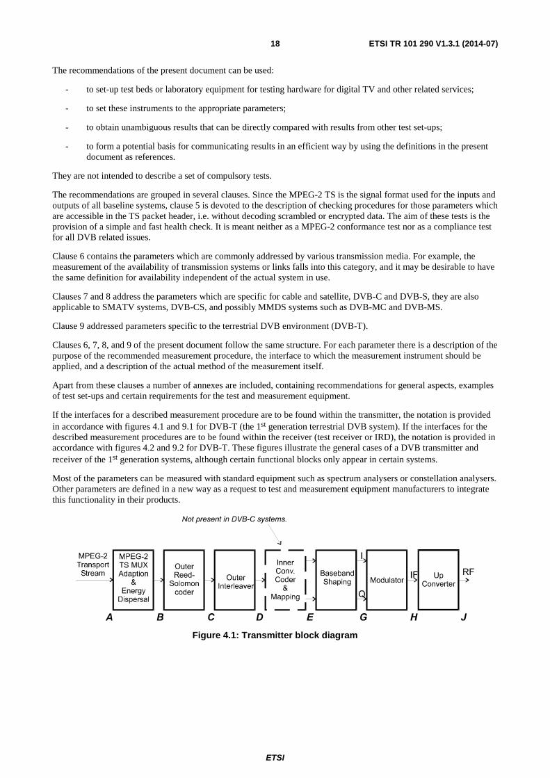
If the interfaces for a described measurement procedure are to be found within the transmitter, the notation is provided in accordance with figures 4.1 and 9.1 for DVB-T (the 1st generation terrestrial DVB system). If the interfaces for the described measurement procedures are to be found within the receiver (test receiver or IRD), the notation is provided in accordance with figures 4.2 and 9.2 for DVB-T. These figures illustrate the general cases of a DVB transmitter and receiver of the 1st generation systems, although certain functional blocks only appear in certain systems.
Most of the parameters can be measured with standard equipment such as spectrum analysers or constellation analysers. Other parameters are defined in a new way as a request to test and measurement equipment manufacturers to integrate this functionality in their products.
Figure 4.1: Transmitter block diagram
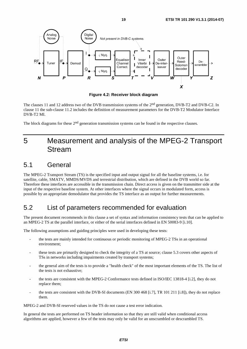
ETSI
ETSI TR 101 290 V1.3.1 (2014-07) 19
Figure 4.2: Receiver block diagram
The clauses 11 and 12 address two of the DVB transmission systems of the 2nd generation, DVB-T2 and DVB-C2. In clause 11 the sub-clause 11.2 includes the definition of measurement parameters for the DVB-T2 Modulator Interface DVB-T2 MI.
The block diagrams for these 2nd generation transmission systems can be found in the respective clauses.
5 Measurement and analysis of the MPEG-2 Transport Stream
5.1 General The MPEG-2 Transport Stream (TS) is the specified input and output signal for all the baseline systems, i.e. for satellite, cable, SMATV, MMDS/MVDS and terrestrial distribution, which are defined in the DVB world so far. Therefore these interfaces are accessible in the transmission chain. Direct access is given on the transmitter side at the input of the respective baseline system. At other interfaces where the signal occurs in modulated form, access is possible by an appropriate demodulator that provides the TS interface as an output for further measurements.
5.2 List of parameters recommended for evaluation The present document recommends in this clause a set of syntax and information consistency tests that can be applied to an MPEG-2 TS at the parallel interface, or either of the serial interfaces defined in EN 50083-9 [i.10].
The following assumptions and guiding principles were used in developing these tests:
- the tests are mainly intended for continuous or periodic monitoring of MPEG-2 TSs in an operational environment;
- these tests are primarily designed to check the integrity of a TS at source; clause 5.3 covers other aspects of TSs in networks including impairments created by transport systems;
- the general aim of the tests is to provide a "health check" of the most important elements of the TS. The list of the tests is not exhaustive;
- the tests are consistent with the MPEG-2 Conformance tests defined in ISO/IEC 13818-4 [i.2], they do not replace them;
- the tests are consistent with the DVB-SI documents (EN 300 468 [i.7], TR 101 211 [i.8]), they do not replace them.
MPEG-2 and DVB-SI reserved values in the TS do not cause a test error indication.
In general the tests are performed on TS header information so that they are still valid when conditional access algorithms are applied, however a few of the tests may only be valid for an unscrambled or descrambled TS.

ETSI
ETSI TR 101 290 V1.3.1 (2014-07) 20
The tests are not dependant on any decoder implementation for consistency of results. The MPEG-2 T-STD model constraints, as defined in ISO/IEC 13818-1 [i.1] (MPEG-2 Systems), should be satisfied as specified in ISO/IEC 13818-4 [i.2] (MPEG-2 Compliance).
Off-line tests are performed under stable conditions, no discontinuity or dynamic change can occur during an off-line test process.
Other digital performance parameters such as BER are not considered in this clause.
This clause tabulates the parameters which are recommended for continuous or periodic monitoring of the MPEG-2 TS.
The tests are grouped into three tables according to their importance for monitoring purposes.
The first table lists a basic set of parameters which are considered necessary to ensure that the TS can be decoded. The second table lists additional parameters which are recommended for continuous monitoring. The third table lists optional additional parameters which could be of interest for certain applications.
Any test equipment intended for the evaluation of these parameters should report test results by means of the indicators itemized in the second column of the tables under exactly the preconditions described in the third column of the tables.
If an indicator is set, then the TS is in error. However, since the indicators do not cover the entire range of possible errors, it cannot be concluded that there is no error if the indicator is not set.
If indicator 1.1 is activated then all other indicators are invalid. Each indicator is activated only as long as at least one of the described preconditions is fulfilled.
NOTE: In the case of indicators requiring a minimum repetition rate of sections, it is intended that each and every section that is present for this table should have the stated repetition rate.
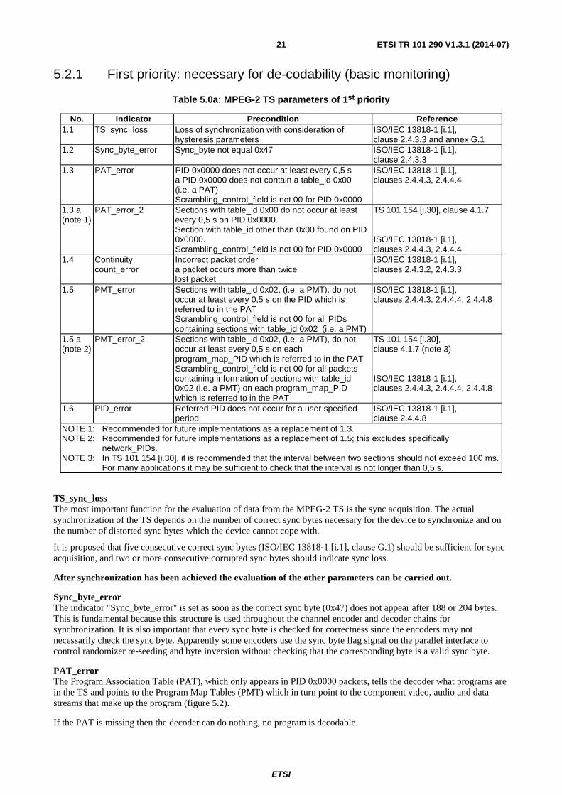
ETSI
ETSI TR 101 290 V1.3.1 (2014-07) 21
5.2.1 First priority: necessary for de-codability (basic monitoring)
Table 5.0a: MPEG-2 TS parameters of 1st priority
No. Indicator Precondition Reference 1.1 TS_sync_loss Loss of synchronization with consideration of
hysteresis parameters ISO/IEC 13818-1 [i.1], clause 2.4.3.3 and annex G.1
1.2 Sync_byte_error Sync_byte not equal 0x47 ISO/IEC 13818-1 [i.1], clause 2.4.3.3
1.3 PAT_error PID 0x0000 does not occur at least every 0,5 s a PID 0x0000 does not contain a table_id 0x00 (i.e. a PAT) Scrambling_control_field is not 00 for PID 0x0000
ISO/IEC 13818-1 [i.1], clauses 2.4.4.3, 2.4.4.4
1.3.a (note 1)
PAT_error_2 Sections with table_id 0x00 do not occur at least every 0,5 s on PID 0x0000. Section with table_id other than 0x00 found on PID 0x0000. Scrambling_control_field is not 00 for PID 0x0000
TS 101 154 [i.30], clause 4.1.7 ISO/IEC 13818-1 [i.1], clauses 2.4.4.3, 2.4.4.4
1.4 Continuity_ count_error
Incorrect packet order a packet occurs more than twice lost packet
ISO/IEC 13818-1 [i.1], clauses 2.4.3.2, 2.4.3.3
1.5 PMT_error Sections with table_id 0x02, (i.e. a PMT), do not occur at least every 0,5 s on the PID which is referred to in the PAT Scrambling_control_field is not 00 for all PIDs containing sections with table_id 0x02 (i.e. a PMT)
ISO/IEC 13818-1 [i.1], clauses 2.4.4.3, 2.4.4.4, 2.4.4.8
1.5.a (note 2)
PMT_error_2 Sections with table_id 0x02, (i.e. a PMT), do not occur at least every 0,5 s on each program_map_PID which is referred to in the PAT Scrambling_control_field is not 00 for all packets containing information of sections with table_id 0x02 (i.e. a PMT) on each program_map_PID which is referred to in the PAT
TS 101 154 [i.30], clause 4.1.7 (note 3) ISO/IEC 13818-1 [i.1], clauses 2.4.4.3, 2.4.4.4, 2.4.4.8
1.6 PID_error Referred PID does not occur for a user specified period.
ISO/IEC 13818-1 [i.1], clause 2.4.4.8
NOTE 1: Recommended for future implementations as a replacement of 1.3. NOTE 2: Recommended for future implementations as a replacement of 1.5; this excludes specifically
network_PIDs. NOTE 3: In TS 101 154 [i.30], it is recommended that the interval between two sections should not exceed 100 ms.
For many applications it may be sufficient to check that the interval is not longer than 0,5 s.
TS_sync_loss The most important function for the evaluation of data from the MPEG-2 TS is the sync acquisition. The actual synchronization of the TS depends on the number of correct sync bytes necessary for the device to synchronize and on the number of distorted sync bytes which the device cannot cope with.
It is proposed that five consecutive correct sync bytes (ISO/IEC 13818-1 [i.1], clause G.1) should be sufficient for sync acquisition, and two or more consecutive corrupted sync bytes should indicate sync loss.
After synchronization has been achieved the evaluation of the other parameters can be carried out.
Sync_byte_error The indicator "Sync_byte_error" is set as soon as the correct sync byte (0x47) does not appear after 188 or 204 bytes. This is fundamental because this structure is used throughout the channel encoder and decoder chains for synchronization. It is also important that every sync byte is checked for correctness since the encoders may not necessarily check the sync byte. Apparently some encoders use the sync byte flag signal on the parallel interface to control randomizer re-seeding and byte inversion without checking that the corresponding byte is a valid sync byte.
PAT_error The Program Association Table (PAT), which only appears in PID 0x0000 packets, tells the decoder what programs are in the TS and points to the Program Map Tables (PMT) which in turn point to the component video, audio and data streams that make up the program (figure 5.2).
If the PAT is missing then the decoder can do nothing, no program is decodable.
ETSI
ETSI TR 101 290 V1.3.1 (2014-07) 22
Nothing other than a PAT should be contained in a PID 0x0000.
PAT_error_2 The reworded description of the error in PAT_error_2 refers to the possibility that the Program Association Table may consist of several (consecutive) sections with the same table_id 0x00.
Continuity_count_error For this indicator three checks are combined. The preconditions "Incorrect packet order" and "Lost packet" could cause problems for IRD which are not equipped with additional buffer storage and intelligence. It is not necessary for the test equipment to distinguish between these two preconditions as they are logically OR-ed, together with the third precondition, into one indicator.
The latter is also covering the packet loss that may occur on ATM links, where one lost ATM packet would cause the loss of a complete MPEG-2 packet.
The precondition "a packet occurs more than twice" may be symptomatic of a deeper problem that the service provider would like to keep under observation.
PMT_error The Program Association Table (PAT) tells the decoder how many programs there are in the stream and points to the PMTs which contain the information where the parts for any given event can be found. Parts in this context are the video stream (normally one) and the audio streams and the data stream (e.g. Teletext). Without a PMT the corresponding program is not decodable.
PID_error It is checked whether there exists a data stream for each PID that occurs. This error might occur where TS are multiplexed, or demultiplexed and again remultiplexed.
The user specified period should not exceed 5 s for video or audio PIDs (see note). Data services and audio services with ISO 639 [i.17] language descriptor with type greater than '0' should be excluded from this 5 s limit.
NOTE: For PIDs carrying other information such as sub-titles, data services or audio services with ISO 639 [i.17] language descriptor with type greater than '0', the time between two consecutive packets of the same PID may be significantly longer.
In principle, a different user specified period could be defined for each PID.

ETSI
ETSI TR 101 290 V1.3.1 (2014-07) 23
5.2.2 Second priority: recommended for continuous or periodic monitoring
Table 5.0b: MPEG-2 TS parameters of 2nd priority
No. Indicator Precondition Reference 2.1 Transport_error Transport_error_indicator in the TS-Header is set
to "1" ISO/IEC 13818-1 [i.1]: clauses 2.4.3.2, 2.4.3.3
2.2 CRC_error CRC error occurred in CAT, PAT, PMT, NIT, EIT, BAT, SDT or TOT table
ISO/IEC 13818-1 [i.1]: clauses 2.4.4, annex A EN 300 468 [i.7]: clause 5.2
2.3 PCR_error (see notes 1 and 2)
PCR discontinuity of more than 100 ms occurring without specific indication. Time interval between two consecutive PCR values more than 40 ms
ISO/IEC 13818-1 [i.1]: clauses 2.4.3.4, 2.4.3.5 ISO/IEC 13818-4 [i.2]: clause 9.11.3 TS 101 154 [i.30]: clause 4.1.5.3
2.3a PCR_repetition_ error (see notes 1 and 2)
Time interval between two consecutive PCR values more than 40 ms
TS 101 154 [i.30]: clause 4.1.5.3
2.3b PCR_discontinuity_ indicator_error
The difference between two consecutive PCR values (PCRi+1 – PCRi) is outside the range of
0...100 ms without the discontinuity_indicator set
ISO/IEC 13818-1 [i.1]: clauses 2.4.3.4, 2.4.3.5 ISO/IEC 13818-4 [i.2]: clause 9.1.1.3
2.4 PCR_accuracy_ error
PCR accuracy of selected programme is not within ±500 ns
ISO/IEC 13818-1 [i.1]: clause 2.4.2.2
2.5 PTS_error (see note 3) PTS repetition period more than 700 ms ISO/IEC 13818-1 [i.1]: clauses 2.4.3.6, 2.4.3.7, 2.7.4
2.6 CAT_error Packets with transport_scrambling_control not 00 present, but no section with table_id = 0x01 (i.e. a CAT) present Section with table_id other than 0x01 (i.e. not a CAT) found on PID 0x0001
ISO/IEC 13818-1 [i.1]: clause 2.4.4
NOTE 1: The old version of PCR_error (2.3) is a combination of the more specific errors PCR_repetition_error (2.3.a) and PCR_discontinuity_indicator_error (2.3.b) by a logical 'or' function. It is kept in the present document for reasons of consistency of existing implementations. For new implementations it is recommended that the indicators 2.3.a and 2.3.b are used only.
NOTE 2: The limitation to 40 ms in the 'Preconditions' of 2.3 PCR_error and 2.3a PCR_repetition_error was removed from TS 101 154 [i.30] in 2005. The respective clause there now refers only to the 100 ms limitation in [i.1] which is recommended to be applied generally.
NOTE 3: The limitation to 700 ms should not be applied to still pictures.
Transport_error The primary Transport_error indicator is Boolean, but there should also be a resettable binary counter which counts the erroneous TS packets. This counter is intended for statistical evaluation of the errors. If an error occurs, no further error indication should be derived from the erroneous packet.
There may be value in providing a more detailed breakdown of the erroneous packets, for example, by providing a separate Transport_error counter for each program stream or by including the PID of each erroneous packet in a log of Transport_error events. Such extra analysis is regarded as optional and not part of this recommendation.
CRC_error The CRC check for the CAT, PAT, PMT, NIT, EIT, BAT, SDT and TOT indicates whether the content of the corresponding table is corrupted. In this case no further error indication should be derived from the content of the corresponding table.
PCR_error The PCRs are used to re-generate the local 27 MHz system clock. If the PCR do not arrive with sufficient regularity then this clock may jitter or drift. The receiver/decoder may even go out of lock. In DVB a repetition period of not more than 100 ms is permitted, previously a maximum of 40ms was recommended (see note 2 in table 5.0b).
PCR_repetition_error The PCRs are used to re-generate the local 27 MHz system clock. If the PCR do not arrive with sufficient regularity then this clock may jitter or drift. The receiver/decoder may even go out of lock. In DVB a repetition period of not more than 100 ms is permitted, previously a maximum of 40ms was recommended (see note 2 in table 5.0b).
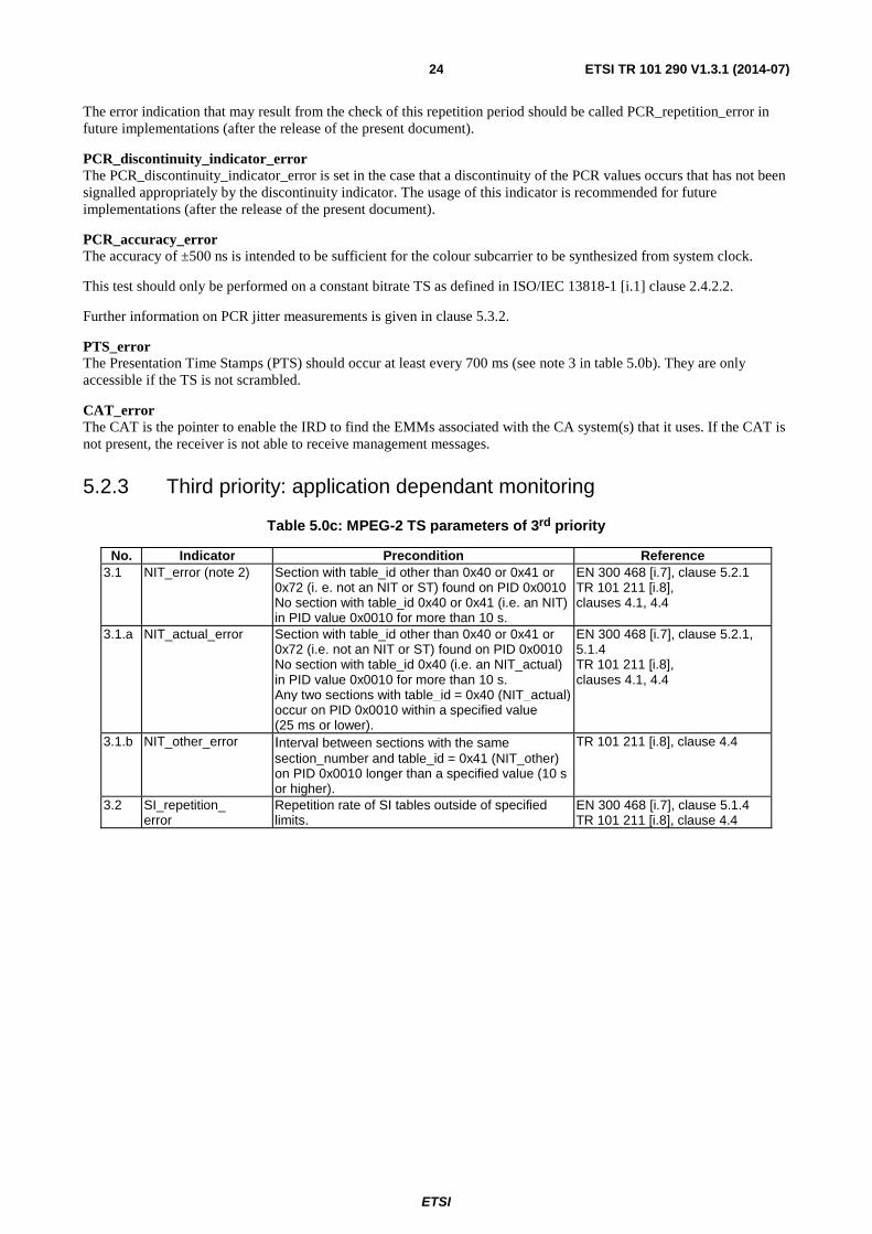
ETSI
ETSI TR 101 290 V1.3.1 (2014-07) 24
The error indication that may result from the check of this repetition period should be called PCR_repetition_error in future implementations (after the release of the present document).
PCR_discontinuity_indicator_error The PCR_discontinuity_indicator_error is set in the case that a discontinuity of the PCR values occurs that has not been signalled appropriately by the discontinuity indicator. The usage of this indicator is recommended for future implementations (after the release of the present document).
PCR_accuracy_error The accuracy of ±500 ns is intended to be sufficient for the colour subcarrier to be synthesized from system clock.
This test should only be performed on a constant bitrate TS as defined in ISO/IEC 13818-1 [i.1] clause 2.4.2.2.
Further information on PCR jitter measurements is given in clause 5.3.2.
PTS_error The Presentation Time Stamps (PTS) should occur at least every 700 ms (see note 3 in table 5.0b). They are only accessible if the TS is not scrambled.
CAT_error The CAT is the pointer to enable the IRD to find the EMMs associated with the CA system(s) that it uses. If the CAT is not present, the receiver is not able to receive management messages.
5.2.3 Third priority: application dependant monitoring
Table 5.0c: MPEG-2 TS parameters of 3rd priority
No. Indicator Precondition Reference 3.1 NIT_error (note 2) Section with table_id other than 0x40 or 0x41 or
0x72 (i. e. not an NIT or ST) found on PID 0x0010 No section with table_id 0x40 or 0x41 (i.e. an NIT) in PID value 0x0010 for more than 10 s.
EN 300 468 [i.7], clause 5.2.1 TR 101 211 [i.8], clauses 4.1, 4.4
3.1.a NIT_actual_error Section with table_id other than 0x40 or 0x41 or 0x72 (i.e. not an NIT or ST) found on PID 0x0010 No section with table_id 0x40 (i.e. an NIT_actual) in PID value 0x0010 for more than 10 s. Any two sections with table_id = 0x40 (NIT_actual) occur on PID 0x0010 within a specified value (25 ms or lower).
EN 300 468 [i.7], clause 5.2.1, 5.1.4 TR 101 211 [i.8], clauses 4.1, 4.4
3.1.b NIT_other_error Interval between sections with the same section_number and table_id = 0x41 (NIT_other) on PID 0x0010 longer than a specified value (10 s or higher).
TR 101 211 [i.8], clause 4.4
3.2 SI_repetition_ error
Repetition rate of SI tables outside of specified limits.
EN 300 468 [i.7], clause 5.1.4 TR 101 211 [i.8], clause 4.4
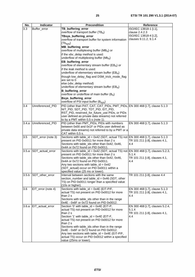
ETSI
ETSI TR 101 290 V1.3.1 (2014-07) 25
No. Indicator Precondition Reference 3.3 Buffer_error TB_buffering_error
overflow of transport buffer (TBn) TBsys_buffering_error overflow of transport buffer for system information (Tbsys) MB_buffering_error overflow of multiplexing buffer (MBn) or if the vbv_delay method is used: underflow of multiplexing buffer (Mbn) EB_buffering_error overflow of elementary stream buffer (EBn) or if the leak method is used: underflow of elementary stream buffer (EBn) though low_delay_flag and DSM_trick_mode_flag are set to 0 else (vbv_delay method) underflow of elementary stream buffer (EBn) B_buffering_error overflow or underflow of main buffer (Bn) Bsys_buffering_error overflow of PSI input buffer (Bsys)
ISO/IEC 13818-1 [i.1], clause 2.4.2.3 ISO/IEC 13818-4 [i.2], clauses 9.11.2, 9.1.4
3.4 Unreferenced_PID PID (other than PAT, CAT, CAT_PIDs, PMT_PIDs, NIT_PID, SDT_PID, TDT_PID, EIT_PID, RST_PID, reserved_for_future_use PIDs, or PIDs user defined as private data streams) not referred to by a PMT within 0,5 s (note 1).
EN 300 468 [i.7], clause 5.1.3
3.4.a Unreferenced_PID PID (other than PMT_PIDs, PIDs with numbers between 0x00 and 0x1F or PIDs user defined as private data streams) not referred to by a PMT or a CAT within 0,5 s.
EN 300 468 [i.7], clause 5.1.3
3.5 SDT_error (note 3) Sections with table_id = 0x42 (SDT, actual TS) not present on PID 0x0011 for more than 2 s Sections with table_ids other than 0x42, 0x46, 0x4A or 0x72 found on PID 0x0011.
EN 300 468 [i.7], clause 5.1.3 TR 101 211 [i.8], clauses 4.1, 4.4
3.5.a SDT_actual_error Sections with table_id = 0x42 (SDT, actual TS) not present on PID 0x0011 for more than 2 s Sections with table_ids other than 0x42, 0x46, 0x4A or 0x72 found on PID 0x0011. Any two sections with table_id = 0x42 (SDT_actual) occur on PID 0x0011 within a specified value (25 ms or lower).
EN 300 468 [i.7], clauses 5.2.3, 5.1.4 TR 101 211 [i.8], clauses 4.1, 4.4
3.5.b SDT_other_error Interval between sections with the same section_number and table_id = 0x46 (SDT, other TS) on PID 0x0011 longer than a specified value (10s or higher).
TR 101 211 [i.8], clause 4.4
3.6 EIT_error (note 4) Sections with table_id = 0x4E (EIT-P/F, actual TS) not present on PID 0x0012 for more than 2 s Sections with table_ids other than in the range 0x4E - 0x6F or 0x72 found on PID 0x0012.
EN 300 468 [i.7], clause 5.1.3 TR 101 211 [i.8], clauses 4.1, 4.4
3.6.a EIT_actual_error Section '0' with table_id = 0x4E (EIT-P, actual TS) not present on PID 0x0012 for more than 2 s Section '1' with table_id = 0x4E (EIT-F, actual TS) not present on PID 0x0012 for more than 2 s Sections with table_ids other than in the range 0x4E - 0x6F or 0x72 found on PID 0x0012. Any two sections with table_id = 0x4E (EIT-P/F, actual TS) occur on PID 0x0012 within a specified value (25ms or lower).
EN 300 468 [i.7], clauses 5.2.4, 5.1.4 TR 101 211 [i.8], clauses 4.1, 4.4

ETSI
ETSI TR 101 290 V1.3.1 (2014-07) 26
No. Indicator Precondition Reference 3.6.b EIT_other_error Interval between sections '0' with table_id = 0x4F
(EIT-P, other TS) on PID 0x0012 longer than a specified value (10s or higher); Interval between sections '1' with table_id = 0x4F (EIT-F, other TS) on PID 0x0012 longer than a specified value (10s or higher).
TR 101 211 [i.8], clause 4.4
3.6.c EIT_PF_error If either section ('0' or '1') of each EIT P/F subtable is present both should exist. Otherwise EIT_PF_error should be indicated.
EN 300 468 [i.7], clause 5.2.4.
3.7 RST_error Sections with table_id other than 0x71 or 0x72 found on PID 0x0013. Any two sections with table_id = 0x71 (RST) occur on PID 0x0013 within a specified value (25 ms or lower).
EN 300 468 [i.7], clause 5.1.3
3.8 TDT_error Sections with table_id = 0x70 (TDT) not present on PID 0x0014 for more than 30 s Sections with table_id other than 0x70, 0x72 (ST) or 0x73 (TOT) found on PID 0x0014. Any two sections with table_id = 0x70 (TDT) occur on PID 0x0014 within a specified value (25 ms or lower).
EN 300 468 [i.7], clauses 5.1.3, 5.2.6 TR 101 211 [i.8], clauses 4.1, 4.4
3.9 Empty_buffer_error Transport buffer (TBn) not empty at least once per second or transport buffer for system information (TBsys) not empty at least once per second or if the leak method is used multiplexing buffer (MBn) not empty at least once per second.
ISO/IEC 13818-1 [i.1], clauses 2.4.2.3, 2.4.2.6 ISO/IEC 13818-9 [i.3], annex E ISO/IEC 13818-4 [i.2], clauses 9.1.1.2, 9.1.4
3.10 Data_delay_error Delay of data (except still picture video data) through the TSTD buffers superior to 1 second; or delay of still picture video data through the TSTD buffers superior to 60 s.
ISO/IEC 13818-1 [i.1], clauses 2.4.2.3, 2.4.2.6
NOTE 1: It is assumed that transition states are limited to 0,5 s, and these transitions should not cause error indications.
NOTE 2: The old version of NIT_error (3.1) has been split into the more specific errors NIT_actual_error (3.1.a) and NIT_other_error (3.1.b). The old version is kept in the document for reasons of consistency of existing implementations. For new implementations it is recommended that the indicators 3.1.a and 3.1.b are used only.
NOTE 3: The old version of SDT_error (3.5) has been split into the more specific errors SDT_actual_error (3.5.a) and SDT_other_error (3.5.b). The old version is kept in the present document for reasons of consistency of existing implementations. For new implementations it is recommended that the indicators 3.5.a and 3.5.b are used only.
NOTE 4: The old version of EIT_error (3.6) has been split into the more specific errors EIT_actual_error (3.6.a), EIT_other_error (3.6.b) and EIT_PF_error (3.6.c). The old version is kept in the present document for reasons of consistency of existing implementations. For new implementations it is recommended that the indicators 3.6.a, 3.6.b and 3.6.c are used only.
NIT_error [i.1] Network Information Tables (NITs) as defined by DVB contain information on frequency, code rates, modulation, polarization, etc. of various programs which the decoder can use. It is checked whether NITs are present in the TS and whether they have the correct PID.
NIT_actual_error Network Information Tables (NITs) as defined by DVB contain information on frequency, code rates, modulation, polarization, etc. of various programs which the decoder can use. It is checked whether the NIT related to the respective TS is present in this TS and whether it has the correct PID.
NIT_other_error Further Network Information Tables (NITs) can be present under a separate PID and refer to other TSs to provide more information on programmes available on other channels. Their distribution is not mandatory and the checks should only be performed if they are present.
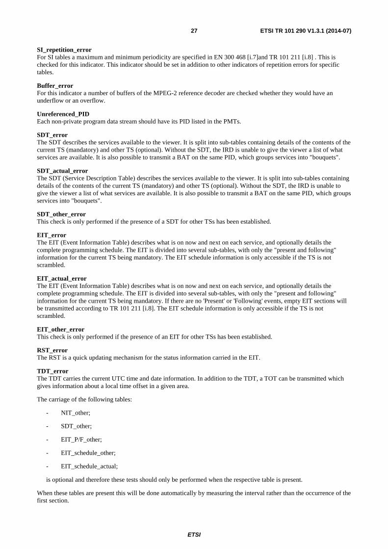
ETSI
ETSI TR 101 290 V1.3.1 (2014-07) 27
SI_repetition_error For SI tables a maximum and minimum periodicity are specified in EN 300 468 [i.7]and TR 101 211 [i.8] . This is checked for this indicator. This indicator should be set in addition to other indicators of repetition errors for specific tables.
Buffer_error For this indicator a number of buffers of the MPEG-2 reference decoder are checked whether they would have an underflow or an overflow.
Unreferenced_PID Each non-private program data stream should have its PID listed in the PMTs.
SDT_error The SDT describes the services available to the viewer. It is split into sub-tables containing details of the contents of the current TS (mandatory) and other TS (optional). Without the SDT, the IRD is unable to give the viewer a list of what services are available. It is also possible to transmit a BAT on the same PID, which groups services into "bouquets".
SDT_actual_error The SDT (Service Description Table) describes the services available to the viewer. It is split into sub-tables containing details of the contents of the current TS (mandatory) and other TS (optional). Without the SDT, the IRD is unable to give the viewer a list of what services are available. It is also possible to transmit a BAT on the same PID, which groups services into "bouquets".
SDT_other_error This check is only performed if the presence of a SDT for other TSs has been established.
EIT_error The EIT (Event Information Table) describes what is on now and next on each service, and optionally details the complete programming schedule. The EIT is divided into several sub-tables, with only the "present and following" information for the current TS being mandatory. The EIT schedule information is only accessible if the TS is not scrambled.
EIT_actual_error The EIT (Event Information Table) describes what is on now and next on each service, and optionally details the complete programming schedule. The EIT is divided into several sub-tables, with only the "present and following" information for the current TS being mandatory. If there are no 'Present' or 'Following' events, empty EIT sections will be transmitted according to TR 101 211 [i.8]. The EIT schedule information is only accessible if the TS is not scrambled.
EIT_other_error This check is only performed if the presence of an EIT for other TSs has been established.
RST_error The RST is a quick updating mechanism for the status information carried in the EIT.
TDT_error The TDT carries the current UTC time and date information. In addition to the TDT, a TOT can be transmitted which gives information about a local time offset in a given area.
The carriage of the following tables:
- NIT_other;
- SDT_other;
- EIT_P/F_other;
- EIT_schedule_other;
- EIT_schedule_actual;
is optional and therefore these tests should only be performed when the respective table is present.
When these tables are present this will be done automatically by measuring the interval rather than the occurrence of the first section.
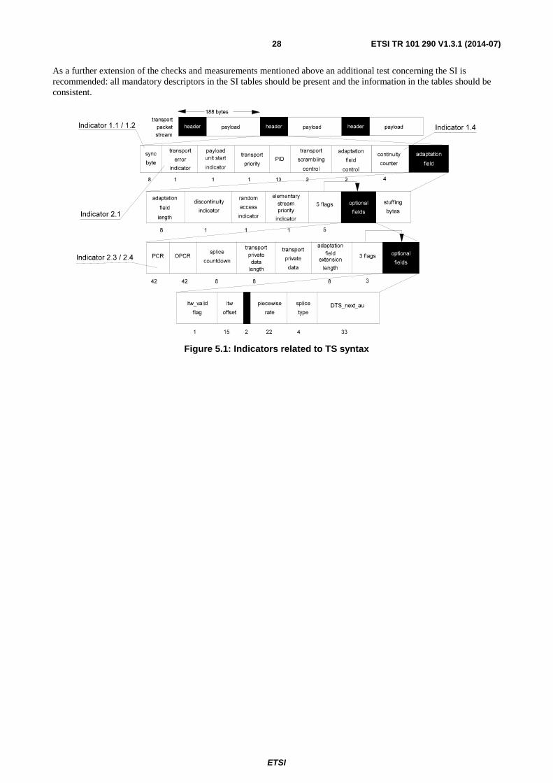
ETSI
ETSI TR 101 290 V1.3.1 (2014-07) 28
As a further extension of the checks and measurements mentioned above an additional test concerning the SI is recommended: all mandatory descriptors in the SI tables should be present and the information in the tables should be consistent.
Figure 5.1: Indicators related to TS syntax
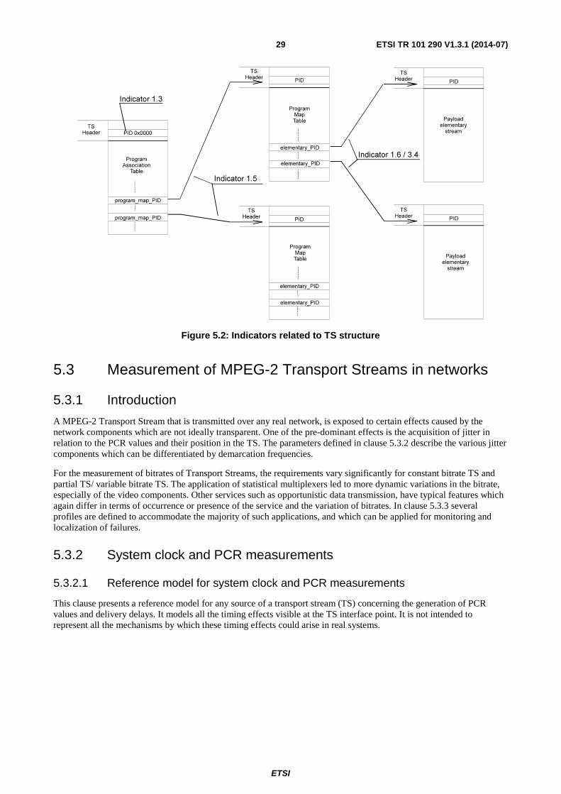
ETSI
ETSI TR 101 290 V1.3.1 (2014-07) 29
Figure 5.2: Indicators related to TS structure
5.3 Measurement of MPEG-2 Transport Streams in networks
5.3.1 Introduction
A MPEG-2 Transport Stream that is transmitted over any real network, is exposed to certain effects caused by the network components which are not ideally transparent. One of the pre-dominant effects is the acquisition of jitter in relation to the PCR values and their position in the TS. The parameters defined in clause 5.3.2 describe the various jitter components which can be differentiated by demarcation frequencies.
For the measurement of bitrates of Transport Streams, the requirements vary significantly for constant bitrate TS and partial TS/ variable bitrate TS. The application of statistical multiplexers led to more dynamic variations in the bitrate, especially of the video components. Other services such as opportunistic data transmission, have typical features which again differ in terms of occurrence or presence of the service and the variation of bitrates. In clause 5.3.3 several profiles are defined to accommodate the majority of such applications, and which can be applied for monitoring and localization of failures.
5.3.2 System clock and PCR measurements
5.3.2.1 Reference model for system clock and PCR measurements
This clause presents a reference model for any source of a transport stream (TS) concerning the generation of PCR values and delivery delays. It models all the timing effects visible at the TS interface point. It is not intended to represent all the mechanisms by which these timing effects could arise in real systems.
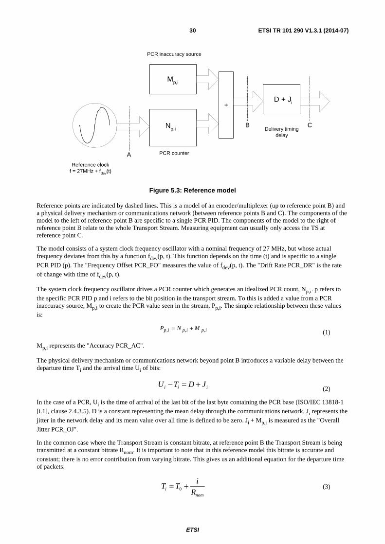
ETSI
ETSI TR 101 290 V1.3.1 (2014-07) 30
Reference clockf = 27MHz + fdev(t)
PCR counter
PCR inaccuracy source
Mp,i
Np,i
+D + Ji
Delivery timingdelay
A
B C
Figure 5.3: Reference model
Reference points are indicated by dashed lines. This is a model of an encoder/multiplexer (up to reference point B) and a physical delivery mechanism or communications network (between reference points B and C). The components of the model to the left of reference point B are specific to a single PCR PID. The components of the model to the right of reference point B relate to the whole Transport Stream. Measuring equipment can usually only access the TS at reference point C.
The model consists of a system clock frequency oscillator with a nominal frequency of 27 MHz, but whose actual frequency deviates from this by a function fdev(p, t). This function depends on the time (t) and is specific to a single
PCR PID (p). The "Frequency Offset PCR_FO" measures the value of fdev(p, t). The "Drift Rate PCR_DR" is the rate
of change with time of fdev(p, t).
The system clock frequency oscillator drives a PCR counter which generates an idealized PCR count, Np,i. p refers to
the specific PCR PID p and i refers to the bit position in the transport stream. To this is added a value from a PCR inaccuracy source, Mp,i to create the PCR value seen in the stream, Pp,i. The simple relationship between these values
is:
ipipip MNP ,,, += (1)
Mp,i represents the "Accuracy PCR_AC".
The physical delivery mechanism or communications network beyond point B introduces a variable delay between the departure time Ti and the arrival time Ui of bits:
iii JDTU +=− (2)
In the case of a PCR, Ui is the time of arrival of the last bit of the last byte containing the PCR base (ISO/IEC 13818-1
[i.1], clause 2.4.3.5). D is a constant representing the mean delay through the communications network. Ji represents the
jitter in the network delay and its mean value over all time is defined to be zero. Ji + Mp,i is measured as the "Overall
Jitter PCR_OJ".
In the common case where the Transport Stream is constant bitrate, at reference point B the Transport Stream is being transmitted at a constant bitrate Rnom. It is important to note that in this reference model this bitrate is accurate and
constant; there is no error contribution from varying bitrate. This gives us an additional equation for the departure time of packets:
nom
i R
iTT += 0 (3)

ETSI
ETSI TR 101 290 V1.3.1 (2014-07) 31
T0 is a constant representing the time of departure of the zero'th bit. Combining equations 2 and 3 we have for the
arrival time:
i
nomi JD
R
iTU +++= 0
(4)
5.3.2.2 Measurement descriptions
The following measurements require a demarcation frequency for delimiting the range of drift rate and jitter frequencies of the timing variations of PCRs and/ or TSs.
The demarcation frequency used should be chosen from table 5.1 and indicated with the measurement results.
Table 5.1: Profiles for jitter and drift rate measurements
Profile Demarcation frequency
Comments
MGF1 10 mHz This profile is provided to give the total coverage of frequency components included in the timing impairments of PCR related measurements. This profile provides the most accurate results in accordance with the limits specified in ISO/IEC 13818-1 [i.1], clause 2.4.2.1. If jitter or drift rate measurements are found out of specification when using other profiles, it is suggested to use this one for better accuracy.
MGF2 100 mHz This profile is accounting for intermediate benefits between the profiles MGF1 and MGF3, by giving reasonable measurement response as well as reasonable account for low frequency components of the timing impairments.
MGF3 1 Hz This profile provides faster measurement response by taking in account only the highest frequency components of the timing impairments. This profile is expected to be sufficient in many applications.
MGF4 Manufacturer defined
This profile will provide any benefit that the manufacturer may consider as useful when it is designed and implemented in a measurement instrument. The demarcation frequency has to be supplied with the measurement result. Optionally any other data that the manufacturer may consider to be relevant may be supplied. For testing against ISO/IEC 13818-9 [i.3] (±25 µs jitter limit) a demarcation frequency of 2 mHz is required. A filter for such demarcation may be implemented under this MGF4 profile.
5.3.2.3 Program Clock Reference - Frequency Offset PCR_FO
Definition PCR_FO is defined as the difference between the program clock frequency and the nominal clock frequency (measured against a reference which is not PCR derived, neither TS derived). The units for the parameter PCR_FO should be in Hz according to:
• Measured Frequency - Nominal Frequency, • or in ppm expressed as:
− [Measured Frequency (in Hz) - Nominal Frequency(in Hz)]/Nominal Frequency (in MHz). Purpose The original frequency of the clock used in the digital video format before compression (program clock) is
transmitted to the final receiver in form of numerical values in the PCR fields. The tolerance as specified by ISO/IEC 13818-1 [i.1] clause 2.4.2.1 is ±810 Hz or ±30 ppm.
Interface A, Z

ETSI
ETSI TR 101 290 V1.3.1 (2014-07) 32
5.3.2.4 Program Clock Reference – Drift Rate PCR_DR
Definition PCR_DR is defined as the first derivative of the frequency and is measured on the low frequency components of the difference between the program clock frequency and the nominal clock frequency (measured against a reference which is not PCR derived, neither TS derived). The format of the parameter PCR_DR should be in mHz/s (@ 27 MHz) or ppm/ hour.
Purpose The measurement is designed to verify that the frequency drift, if any, of the program clock frequency is below the limits set by ISO/IEC 13818-1 [i.1]. This limit is effective only for the low frequency components of the variations. The tolerance as specified by ISO/IEC 13818-1 [i.1] is ±75 mHz/s@ 27 MHz or ±10 ppm/ hour.
Interface A, Z NOTE: A break frequency of 10 mHz is recommended for the separation of PCR_jitter (higher frequencies) and
PCR_drift (lower frequencies). See also MGF1 in Table 5.1.
5.3.2.5 Program Clock Reference - Overall Jitter PCR_OJ
Definition PCR_OJ is defined as the instantaneous measurement of the high frequency components of the difference between when a PCR should have arrived at a measurement point (based upon previous PCR values, its own value and a reference which is not PCR or TS derived) and when it did arrive. The format of the parameter PCR_OJ should be in nanoseconds.
Purpose The PCR_OJ measurement is designed to account for all cumulative errors affecting the PCR values during program stream generation, multiplexing, transmission, etc. All these effects appear as jitter at the receiver but they are a combination of PCR inaccuracies and jitter in the transmission. This value can be compared against the maximum error specification by ISO/IEC 13818-1 [i.1] for PCR Accuracy of ±500 ns only if the jitter in the transmission is assumed to be zero.
Interface A, Z NOTE: A break frequency of 10 mHz is recommended for the separation of PCR_jitter (higher frequencies) and
PCR_drift (lower frequencies). See also MGF1 in table 5.1.
5.3.2.6 Program Clock Reference – Accuracy PCR_AC
Definition The accuracy of the PCR values PCR_AC is defined as the difference between the actual PCR value and the value it should have in the TS represented by the byte index for its actual position. This can be calculated for constant bitrate TS, the measurement may NOT produce meaningful results in variable bitrate TS. The units for the parameter PCR_AC should be in nanoseconds.
Purpose This measurement is designed to indicate the total error included in the PCR value with respect to its position in the TS. The tolerance as specified by ISO/IEC 13818-1 [i.1] is ±500 ns. This measurement is considered to be valid for both: real time and off-line measurements. The measurement should trigger the indicator under paragraph 5.2.2. item 2.4.
Interface A. Z
NOTE: Note that PCR Accuracy is defined by ISO/IEC 13818-1 [i.1]: "A tolerance is specified for the PCR values. The PCR tolerance is defined as the maximum inaccuracy allowed received PCRs. This inaccuracy may be due to imprecision in the PCR values or to PCR modification during re-multiplexing. It does not include errors in packet arrival time due to network jitter or other causes".
5.3.3 Bitrate measurement
The bitrate value from a measurement system depends on a number of parameters:
- when the bitrate measurement is started;
- what is counted (packets, bytes, bits);
- the time duration (gate) over which the bitrate is measured;
- the way in which the time-gate function moves between measurements (timeSlice).
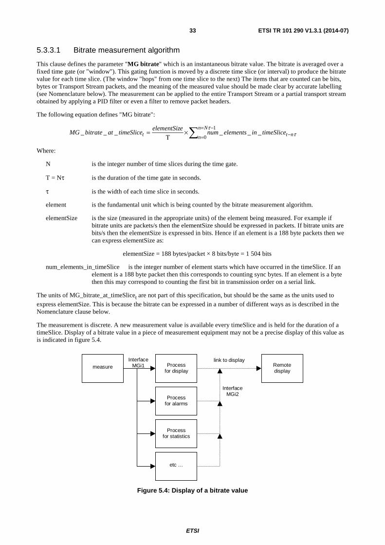
ETSI
ETSI TR 101 290 V1.3.1 (2014-07) 33
5.3.3.1 Bitrate measurement algorithm
This clause defines the parameter "MG bitrate" which is an instantaneous bitrate value. The bitrate is averaged over a fixed time gate (or "window"). This gating function is moved by a discrete time slice (or interval) to produce the bitrate value for each time slice. (The window "hops" from one time slice to the next) The items that are counted can be bits, bytes or Transport Stream packets, and the meaning of the measured value should be made clear by accurate labelling (see Nomenclature below). The measurement can be applied to the entire Transport Stream or a partial transport stream obtained by applying a PID filter or even a filter to remove packet headers.
The following equation defines "MG bitrate":
∑
−=
= −×Τ
=1
0______
ττ
Nn
n ntt timeSliceinelementsnumeelementSiz
timeSliceatbitrateMG
Where:
N is the integer number of time slices during the time gate.
T = Nτ is the duration of the time gate in seconds.
τ is the width of each time slice in seconds.
element is the fundamental unit which is being counted by the bitrate measurement algorithm.
elementSize is the size (measured in the appropriate units) of the element being measured. For example if bitrate units are packets/s then the elementSize should be expressed in packets. If bitrate units are bits/s then the elementSize is expressed in bits. Hence if an element is a 188 byte packets then we can express elementSize as:
elementSize = 188 bytes/packet × 8 bits/byte = 1 504 bits
num_elements_in_timeSlice is the integer number of element starts which have occurred in the timeSlice. If an element is a 188 byte packet then this corresponds to counting sync bytes. If an element is a byte then this may correspond to counting the first bit in transmission order on a serial link.
The units of MG_bitrate_at_timeSlicet are not part of this specification, but should be the same as the units used to
express elementSize. This is because the bitrate can be expressed in a number of different ways as is described in the Nomenclature clause below.
The measurement is discrete. A new measurement value is available every timeSlice and is held for the duration of a timeSlice. Display of a bitrate value in a piece of measurement equipment may not be a precise display of this value as is indicated in figure 5.4.
measure Processfor display
Processfor alarms
Processfor statistics
etc …
link to displayRemotedisplay
InterfaceMGi1
InterfaceMGi2
Figure 5.4: Display of a bitrate value

ETSI
ETSI TR 101 290 V1.3.1 (2014-07) 34
5.3.3.2 Preferred values for Bitrate Measurement
The preferred values for the algorithm are application dependent. One set of values may be appropriate for monitoring and another may be appropriate for precise measurements. In order to have consistent measurements between different equipment vendors, the following profiles are defined. (Note that the timeSlice interval τ can be expressed as a time or as a frequency for precision).
Table 5.1a: Preferred profiles for bitrate measurements
MG Profile
Profile Description Stream Type/Rate τ N T=Nτ element
MGB1 This Profile is best geared towards applications where the bitrate is constant or slowly varying. It is compatible with much equipment developed before this specification was created.
All 1 s 1 1 s 188 byte packet
MGB2 This Profile provides overall consistent rate calculations while providing reasonable accuracy for most monitoring and troubleshooting applications. It is intended for CBR measurements whereas rapidly varying bitrates are more appropriately measured with the MGB3 or MGB4 profiles.
All 100 ms 10 1 s 188 byte packet
MGB3 This Profile provides for tracking of small variations in the multiplex rate of each element.
All 1/90 kHz 1 800 20 ms 188 byte packet
MGB4 This Profile provides for a longer term average for rate calculation but with repeatability between two different measurements of the same data.
All 1/90 kHz 9×10⁴ 1 s 188 byte packet
MGB5 This Profile allows the user to tune bitrate calculations based on the parameters that are most appropriate for a particular transport stream. It is very important that when this is done, the nomenclature used to define the bitrate clearly shows that bitrates for components are not directly comparable with each other: TS@MGB1 video@MGB3 audio@MGB4 the_rest@188,1s,100s etc. This follows the nomenclature guide in this specification and shows that it is unlikely that the sum of the bitrates of the TS components will equal the overall transport stream rate.
Complete or partial transport stream
User Def. User Def.
User Def.
188 byte packet
Applications of the profiles are given in the informative annex J.
5.3.3.3 Nomenclature
It is important to display bitrate values in a way which allows comparison. Correct nomenclature can indicate for example that correction factors need to be applied to convert from a 204 byte packet bitrate measurement to a 188 byte packet measurement. This recommendation is for the "MG-bitrate" nomenclature. If the "MG bitrate" algorithm has been used, then bitrates are of the form:
<bitrate_value> <units>@ MGprofile
or <bitrate_value> <units> @ MG<element>, <timeslice>, <time_gate> [,<filter>]

ETSI
ETSI TR 101 290 V1.3.1 (2014-07) 35
For example if the full transport stream bitrate of a 204 byte packet system is to be measured, then it is important to know the size of the packet (i.e. the elementSize) and the size of the time window which was measured to ensure repeatability. Hence a bitrate should be expressed as:
10,300 Mbit/s @ MG 204,1/90 kHz,1,1s example 1
It is assumed by default that the bitrate was for the full transport stream.
If the bitrate of all the service components for a service called "Test Transmission" (i.e. all PIDs listed in the PMT + the bitrate of the PMT excluding the bitrate of EITp and EITf for that service) is to be measured, then it would be expressed as:
4,154 Mbit/s @ MG 188, 1/90 kHz,1s,service: Test Transmission example 2
or 4,154 Mbit/s @ MGB4, service: Test Transmission
To express example 2 as a percentage of the total bitrate in example 1, it is obvious now that a 188/204 correction factor needs to be applied before the division takes place:
Test Transmission = 100 × (4,154 × 204/188 )/10,300 % of bitrate
43,8 % of bitrate
Note that this nomenclature is independent of the measurement technique, but is vital to allow results to be compared.
Note also that when writing MG-bitrate measurements, the values kbit/s and Mbit/s are taken to mean 103 bits per second and 106 bits per second respectively. It is also recommended that the values kB/s (103 bytes/s) and MB/s (106 bytes/s) are not used.
5.3.4 Consistency of information check
The information provided in the various SI/ PSI tables in different Transport Streams needs to be consistent and coherent to provide access to all services for the user. Wherever these tables are created, modified or extracted, there is a need for checking the tables of the outgoing Transport Stream.
In many cases, these applications are user-defined in the sense that providers and operators may wish to minimize the complexity of these checks.
As a first example for such a check, the Transport_Stream_ID check is defined hereafter.
5.3.4.1 Transport_Stream_ID check
Definition Each MPEG-2 Transport Stream should be identifiable by its Transport_Stream_ID carried in the PAT. Purpose As DVB networks become more and more complex, there is an increased risk of transmitting the wrong
Transport Stream. Providers and operators may wish to make sure that the TS they actually process is the intended one.
Interface A, Z Method The Transport Stream ID (as referenced in the PAT) should be checked and the actual TS ID should be
compared with a user defined value. By this it can be tested whether the actual Transport Stream is the correct one.
5.3.5 TS parameters in transmission systems with reduced SI data
Certain transmission systems, e.g. DSNG Transport Streams conforming to EN 301 210 [i.18] contain simplified PSI/SI information (see annex D of EN 301 210 [i.18]. When testing such Transport Streams, table 5.1b indicates which of the tests recommended in clause 5.2 can be used.

ETSI
ETSI TR 101 290 V1.3.1 (2014-07) 36
Table 5.1b: TS parameters in systems with reduced SI data
No. Indicator Comment 1.1 TS_sync_loss Essential for access to TS data 1.2 Sync_byte_error May not necessarily prevent
decoding of content 1.3 PAT_error Essential for access to TS data 1.3.a PAT_error_2 Essential for access to TS data 1.4 Continuity_count_error May not necessarily prevent
decoding of content 1.5 PMT_error Essential for access to TS data 1.5.a PMT_error_2 Essential for access to TS data 1.6 PID_error May not necessarily prevent
decoding of content 2.1 Transport_error 2.2 CRC_error Applies to PAT and PMT only 2.3 PCR_error 2.3a PCR_repetition_error 2.3b PCR_discontinuity_indicator_error 2.4 PCR_accuracy_error 2.5 PTS_error 2.6 CAT_error 3.3 Buffer_error 3.4 Unreferenced_PID 3.4.a Unreferenced_PID 3.9 Empty_buffer_error 3.10 Data_delay_error
5.4 Measurement of availability at MPEG-2 Transport Stream level
Definitions of error events
The following definitions are used to establish criteria for System Availability, Link Availability, and System Error Performance (e.g. for coverage measurement purposes) for distribution networks such as satellite (DVB-S and DVB-DSNG), cable (DVB-C), terrestrial (DVB-T) and microwave systems (DVB-MS, DVB-MC and DVB-MT) as well as for contribution networks (DVB-PDH ETS 300 813 [i.19] and DVB-SDH ETS 300 814 [i.20]).
These definitions may also be used to test the performance of TSs in IRDs via Common Interfaces.

ETSI
ETSI TR 101 290 V1.3.1 (2014-07) 37
Table 5.2: Error Events
5.4.1 Severely Disturbed Period (SDP):
A period of sync loss (as defined in clause 5.2.1 of the present document, parameter 1.1) or loss of signal.
5.4.2 Errored Block (EB): An MPEG-2 TS packet with one or more uncorrectable errors, which is indicated by the transport_error_indicator flag set. See clause 5.2.2.
5.4.3 Errored Time Interval (ETI): A given time interval with one or more EBs. 5.4.3.a Errored Second (ES): A specific case of the ETI where the given time interval is one
second. 5.4.4 Severely Errored Time Interval
(SETI): A given time interval which contains greater than a specified percentage of errored blocks, or at least one SDP or part thereof. This percentage will not be specified in the present document, but should be the subject of agreements between the network operators and the program providers.
5.4.4a Severely Errored Second (SES):
A specific case of the SETI where the given time interval is one second.
5.4.5 Unavailable Time UAT A start of a period of Unavailable Time can be defined as: • either the onset of N consecutive SES/ SETI events; or • the onset of a rolling window of length T in which M SES/
SETI events occur. These time intervals/ seconds are considered to be part of the Unavailable Time. A end of period of Unavailable Time can be defined accordingly as
• the onset of N consecutive non-SES/ SETI events; or • the onset of a rolling window of length T in which no SES/
SETI events occur. These time intervals/ seconds are considered to be part of Available Time. The values N, M and T could differ for different types of service (video, audio, data, etc.).
Note that these tests are only possible if Reed-Solomon encoding was used upstream with respect to the measurement point.
5.5 Evaluation of service performance by combination of TS related parameters
Void.
5.6 Parameters for CI related applications The Common Interface (CI) is - in principle - a Transport Stream interface but it has particular properties which require additional tests.
The parameters defined in this clause are intended to enable reproducible and comparable measurements on the CI. As in the previous clauses on Transport Stream related tests and measurements, it cannot be assumed that these tests provide a complete analysis. They are also designed as a 'health check', not as an overall compliance or conformance test.
The following reference model pictures the interfaces and the functional blocks which are referred to in the definitions of the tests.
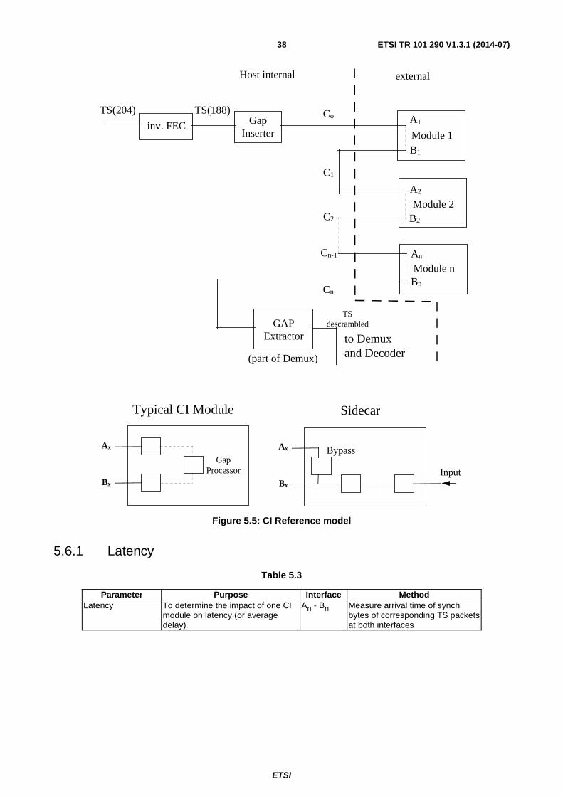
ETSI
ETSI TR 101 290 V1.3.1 (2014-07) 38
TS(204)
inv. FEC
TS(188)Gap
Inserter Module 1
TSdescrambled
to Demuxand Decoder (part of Demux)
Host internal external
Module 2
Module n
A1
B1
A2
B2
An
Bn
Co
Cn
C1
C2
GAPExtractor
Cn-1
Typical CI Module
Bx
Ax
GapProcessor
Bx
Ax Bypass
Input
Sidecar
Figure 5.5: CI Reference model
5.6.1 Latency
Table 5.3
Parameter Purpose Interface Method Latency To determine the impact of one CI
module on latency (or average delay)
An - Bn Measure arrival time of synch bytes of corresponding TS packets at both interfaces
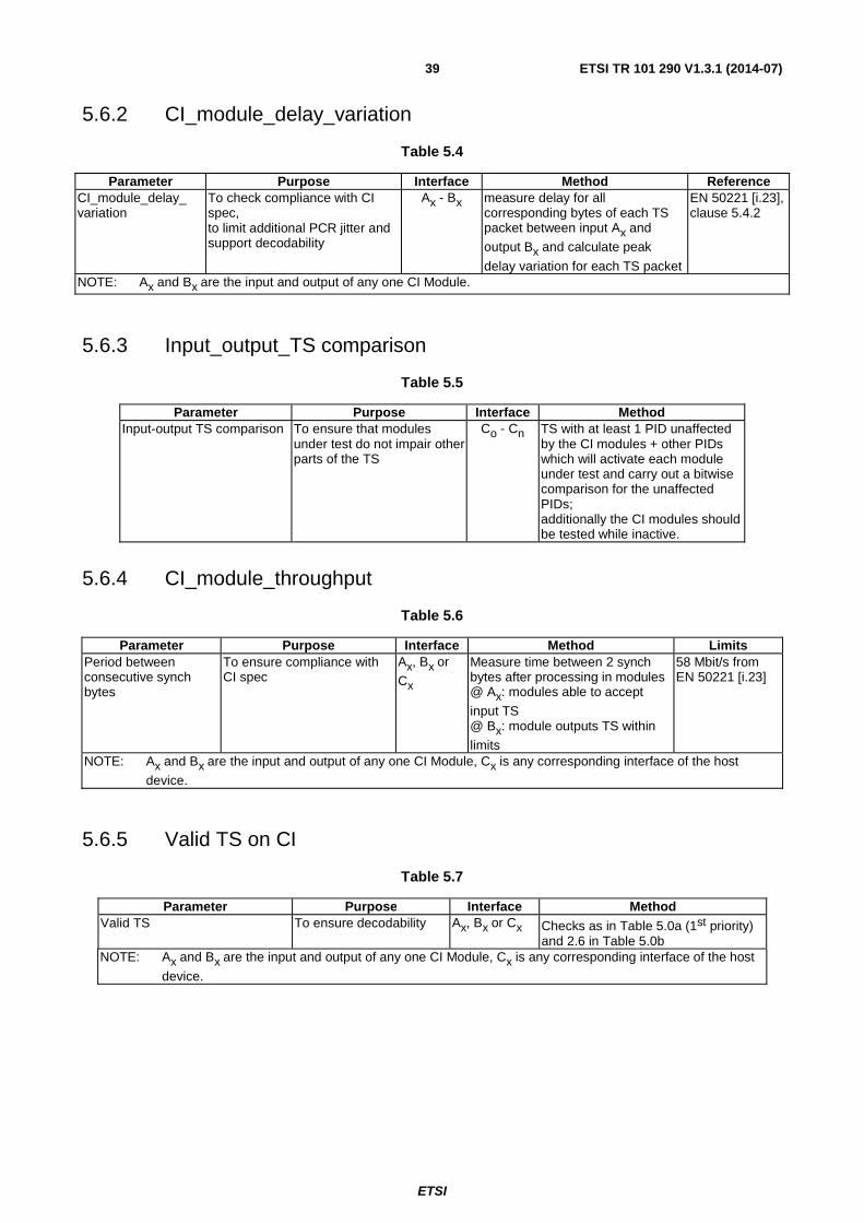
ETSI
ETSI TR 101 290 V1.3.1 (2014-07) 39
5.6.2 CI_module_delay_variation
Table 5.4
Parameter Purpose Interface Method Reference CI_module_delay_ variation
To check compliance with CI spec, to limit additional PCR jitter and support decodability
Ax - Bx measure delay for all corresponding bytes of each TS packet between input Ax and
output Bx and calculate peak
delay variation for each TS packet
EN 50221 [i.23], clause 5.4.2
NOTE: Ax and Bx are the input and output of any one CI Module.
5.6.3 Input_output_TS comparison
Table 5.5
Parameter Purpose Interface Method Input-output TS comparison To ensure that modules
under test do not impair other parts of the TS
Co - Cn TS with at least 1 PID unaffected by the CI modules + other PIDs which will activate each module under test and carry out a bitwise comparison for the unaffected PIDs; additionally the CI modules should be tested while inactive.
5.6.4 CI_module_throughput
Table 5.6
Parameter Purpose Interface Method Limits Period between consecutive synch bytes
To ensure compliance with CI spec
Ax, Bx or
Cx Measure time between 2 synch bytes after processing in modules @ Ax: modules able to accept
input TS @ Bx: module outputs TS within
limits
58 Mbit/s from EN 50221 [i.23]
NOTE: Ax and Bx are the input and output of any one CI Module, Cx is any corresponding interface of the host
device.
5.6.5 Valid TS on CI
Table 5.7
Parameter Purpose Interface Method Valid TS To ensure decodability Ax, Bx or Cx Checks as in Table 5.0a (1st priority)
and 2.6 in Table 5.0b NOTE: Ax and Bx are the input and output of any one CI Module, Cx is any corresponding interface of the host
device.

ETSI
ETSI TR 101 290 V1.3.1 (2014-07) 40
6 Common parameters for satellite and cable transmission media
6.1 System availability Purpose The system availability describes the long-term quality of the complete digital transmission system from
MPEG-2 encoder to the measurement point. Interface Z Method The definition of System Availability is based on the list of performance parameters of table 5.2:
Severely Disturbed Period (SDP) Errored Block (EB) Errored Time Interval ETI/ Errored Second (ES) Severely Errored Time Interval SETI/ Severely Errored Second (SES) Unavailable Time UAT The System Availability is defined as the ratio of (Total Time - Unavailable Time) to Total Time.
6.2 Link availability Purpose The link availability describes the long term quality of a specified link in a digital transmission chain. It could
be used as a quality of service parameter in contracts between network operators and program providers. Interface X (Overload indicator of the Reed Solomon decoder). Method The definition of Link availability is based on following performance parameters:
Uncorrectable Packet (UP) An MPEG-2 TS packet with an uncorrectable error, which is indicated by overload at the Reed-Solomon decoder.
Uncorrectable Time Interval UTI/ Uncorrectable Second (US)
A given time interval with one or more UPs. The US is a specific case of the UTI where the given time interval is one second.
Severely Uncorrectable Time Interval (SUTI)/ Severely Uncorrectable Second (SUS):
A given time interval which contains greater than a specified percentage of Uncorrectable Packets, or at least one SDP (see clause 5.4) or part thereof. NOTE: This percentage will not be specified in the present
document, but should be the subject of agreements between the network operators and the service providers.
The SUS is a specific case of the SUTI where the given time interval is one second.
Link Unavailable Time LUAT A start of a period of Link Unavailable Time can be defined as: • either the onset of N consecutive SUS/ SUTI events; or • the onset of a rolling window of length T in which M
SUS/SUTI events occur. These time intervals/ seconds are considered to be part of the Link Unavailable Time. A end of period of Link Unavailable Time can be defined accordingly as:
• the onset of N consecutive non-SUS/SUTI events; or • the onset of a rolling window of length T in which no
SUS/SUTI events occur. These time intervals/ seconds are considered to be part of Link Available Time. The values N, M and T could differ for different types of service (video, audio, data, etc.).
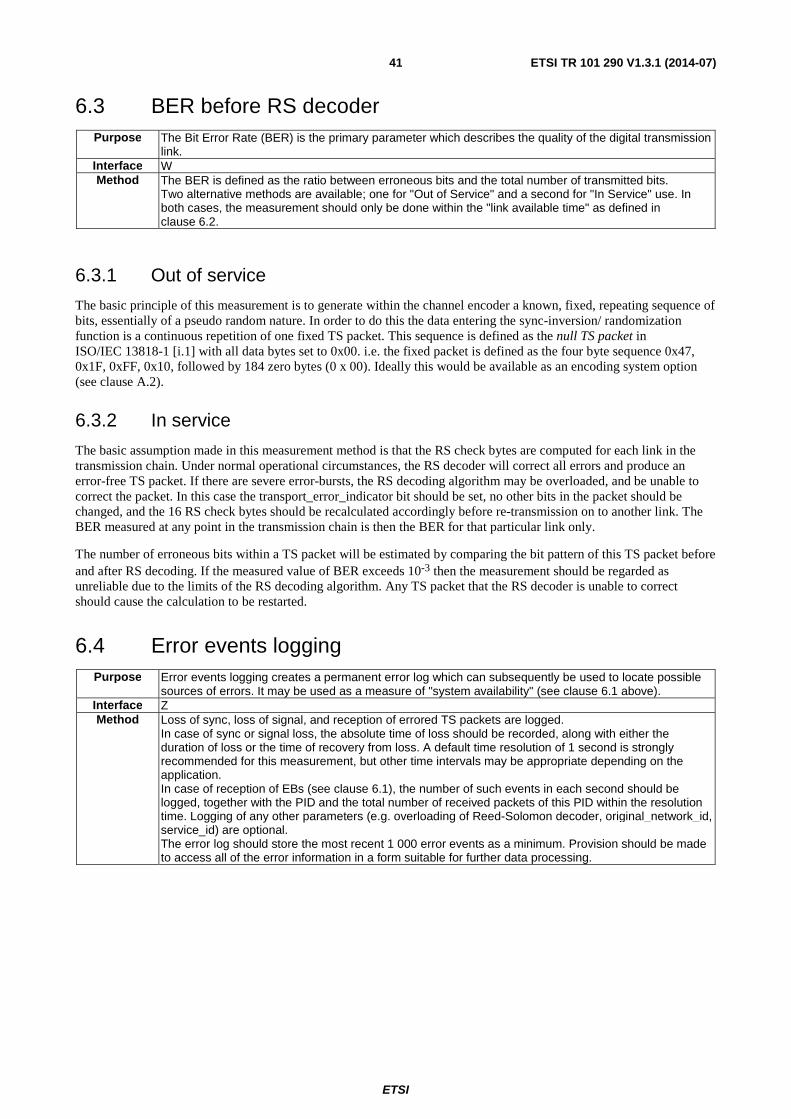
ETSI
ETSI TR 101 290 V1.3.1 (2014-07) 41
6.3 BER before RS decoder Purpose The Bit Error Rate (BER) is the primary parameter which describes the quality of the digital transmission
link. Interface W Method The BER is defined as the ratio between erroneous bits and the total number of transmitted bits.
Two alternative methods are available; one for "Out of Service" and a second for "In Service" use. In both cases, the measurement should only be done within the "link available time" as defined in clause 6.2.
6.3.1 Out of service
The basic principle of this measurement is to generate within the channel encoder a known, fixed, repeating sequence of bits, essentially of a pseudo random nature. In order to do this the data entering the sync-inversion/ randomization function is a continuous repetition of one fixed TS packet. This sequence is defined as the null TS packet in ISO/IEC 13818-1 [i.1] with all data bytes set to 0x00. i.e. the fixed packet is defined as the four byte sequence 0x47, 0x1F, 0xFF, 0x10, followed by 184 zero bytes (0 x 00). Ideally this would be available as an encoding system option (see clause A.2).
6.3.2 In service
The basic assumption made in this measurement method is that the RS check bytes are computed for each link in the transmission chain. Under normal operational circumstances, the RS decoder will correct all errors and produce an error-free TS packet. If there are severe error-bursts, the RS decoding algorithm may be overloaded, and be unable to correct the packet. In this case the transport_error_indicator bit should be set, no other bits in the packet should be changed, and the 16 RS check bytes should be recalculated accordingly before re-transmission on to another link. The BER measured at any point in the transmission chain is then the BER for that particular link only.
The number of erroneous bits within a TS packet will be estimated by comparing the bit pattern of this TS packet before and after RS decoding. If the measured value of BER exceeds 10-3 then the measurement should be regarded as unreliable due to the limits of the RS decoding algorithm. Any TS packet that the RS decoder is unable to correct should cause the calculation to be restarted.
6.4 Error events logging Purpose Error events logging creates a permanent error log which can subsequently be used to locate possible
sources of errors. It may be used as a measure of "system availability" (see clause 6.1 above). Interface Z Method Loss of sync, loss of signal, and reception of errored TS packets are logged.
In case of sync or signal loss, the absolute time of loss should be recorded, along with either the duration of loss or the time of recovery from loss. A default time resolution of 1 second is strongly recommended for this measurement, but other time intervals may be appropriate depending on the application. In case of reception of EBs (see clause 6.1), the number of such events in each second should be logged, together with the PID and the total number of received packets of this PID within the resolution time. Logging of any other parameters (e.g. overloading of Reed-Solomon decoder, original_network_id, service_id) are optional. The error log should store the most recent 1 000 error events as a minimum. Provision should be made to access all of the error information in a form suitable for further data processing.
ETSI
ETSI TR 101 290 V1.3.1 (2014-07) 42
6.5 Transmitter symbol clock jitter and accuracy Purpose Inaccuracies of the symbol clock concerning absolute frequency, frequency drift and jitter may introduce
intersymbol interference. Additionally, the accuracy of transmitted clock references like the Program Clock Reference (PCR) can be influenced. Therefore the degradation of signal quality due to symbol clock inaccuracies has to be negligible. Symbol clock jitter and accuracy can be degraded if the symbol clock is directly synthesized from an unstable TS data clock. For this reason, the measurement should be performed while the transmitter is driven by a TS to ensure a worst case measurement is obtained.
Interface E Method For measurements the absolute frequency, frequency wander and timing jitter are of interest. A PLL
circuit can be used for synchronization to the symbol clock and according to the loop bandwidth, timing jitter is suppressed and low frequency drift (wander) is still present at the output of the loop oscillator. Jitter can be measured with an oscilloscope by triggering with the extracted clock. Jitter is usually expressed as a peak-to-peak value in UI (Unit Interval) where one UI is equal to one clock cycle (Tsymbol). For measurements of the absolute frequency and frequency wander the output of the clock
extractor can be used or the symbol clock can be measured directly using an appropriate frequency counter. NOTE: This measurement refers to the physical layer of TS interconnection. See clause 5.3.2 for
PCR measurements.
6.6 RF/IF signal power Purpose Level measurement is needed to set up a network. Interface Any RF/IF interface, N, P. Method The signal power, or wanted power, is defined as the mean power of the selected signal as would be
measured with a thermal power sensor. Care should be taken to limit the measurement to the bandwidth of the wanted signal. When using a spectrum analyser or a calibrated receiver, it should integrate the signal power within the nominal bandwidth of the signal (symbol rate x(1 + α)).
6.7 Noise power Purpose Noise is a significant impairment in a transmission network. Interface N (out of service) or T (in service) Method The noise power (mean power), or unwanted power, is measured with a spectrum analyser (out of
service) or an estimate is obtained from the IQ diagram (in service), see clause 6.9.9. The noise level is specified using either the occupied bandwidth of the signal, which is equal to the symbol rate x (1 + α). See annex G.
6.8 Bit error count after RS Purpose To measure whether the MPEG-2 TS is quasi error free. Interface Z Method The same principle as used for the "Out of service measurement" of the "BER before the
Reed-Solomon decoder" described in clause 6.3.2, with the modification that the result is presented as an error count rather than a ratio. The receiver only has to compare the received TS packets with the Null packets as defined in clause A.2.
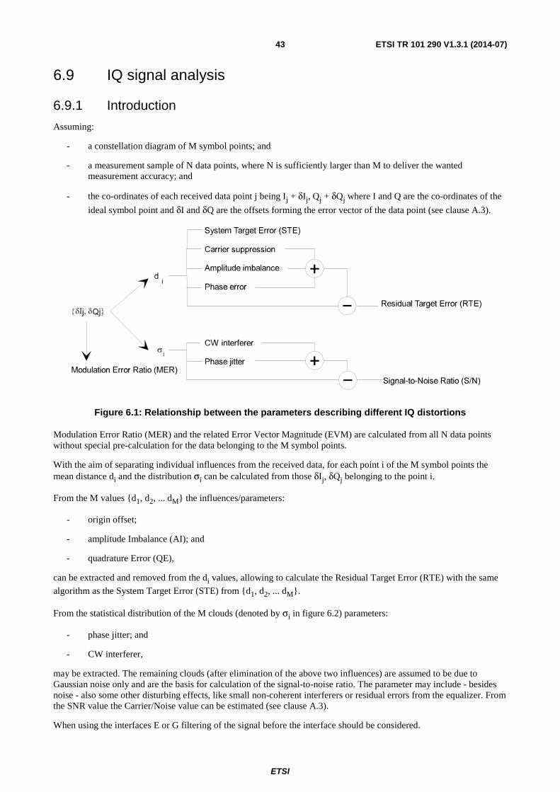
ETSI
ETSI TR 101 290 V1.3.1 (2014-07) 43
6.9 IQ signal analysis
6.9.1 Introduction
Assuming:
- a constellation diagram of M symbol points; and
- a measurement sample of N data points, where N is sufficiently larger than M to deliver the wanted measurement accuracy; and
- the co-ordinates of each received data point j being Ij + δIj, Qj + δQj where I and Q are the co-ordinates of the
ideal symbol point and δI and δQ are the offsets forming the error vector of the data point (see clause A.3).
Figure 6.1: Relationship between the parameters describing different IQ distortions
Modulation Error Ratio (MER) and the related Error Vector Magnitude (EVM) are calculated from all N data points without special pre-calculation for the data belonging to the M symbol points.
With the aim of separating individual influences from the received data, for each point i of the M symbol points the mean distance di and the distribution σi can be calculated from those δIj, δQj belonging to the point i.
From the M values {d1, d2, ... dM} the influences/parameters:
- origin offset;
- amplitude Imbalance (AI); and
- quadrature Error (QE),
can be extracted and removed from the di values, allowing to calculate the Residual Target Error (RTE) with the same
algorithm as the System Target Error (STE) from {d1, d2, ... dM}.
From the statistical distribution of the M clouds (denoted by σi in figure 6.2) parameters:
- phase jitter; and
- CW interferer,
may be extracted. The remaining clouds (after elimination of the above two influences) are assumed to be due to Gaussian noise only and are the basis for calculation of the signal-to-noise ratio. The parameter may include - besides noise - also some other disturbing effects, like small non-coherent interferers or residual errors from the equalizer. From the SNR value the Carrier/Noise value can be estimated (see clause A.3).
When using the interfaces E or G filtering of the signal before the interface should be considered.
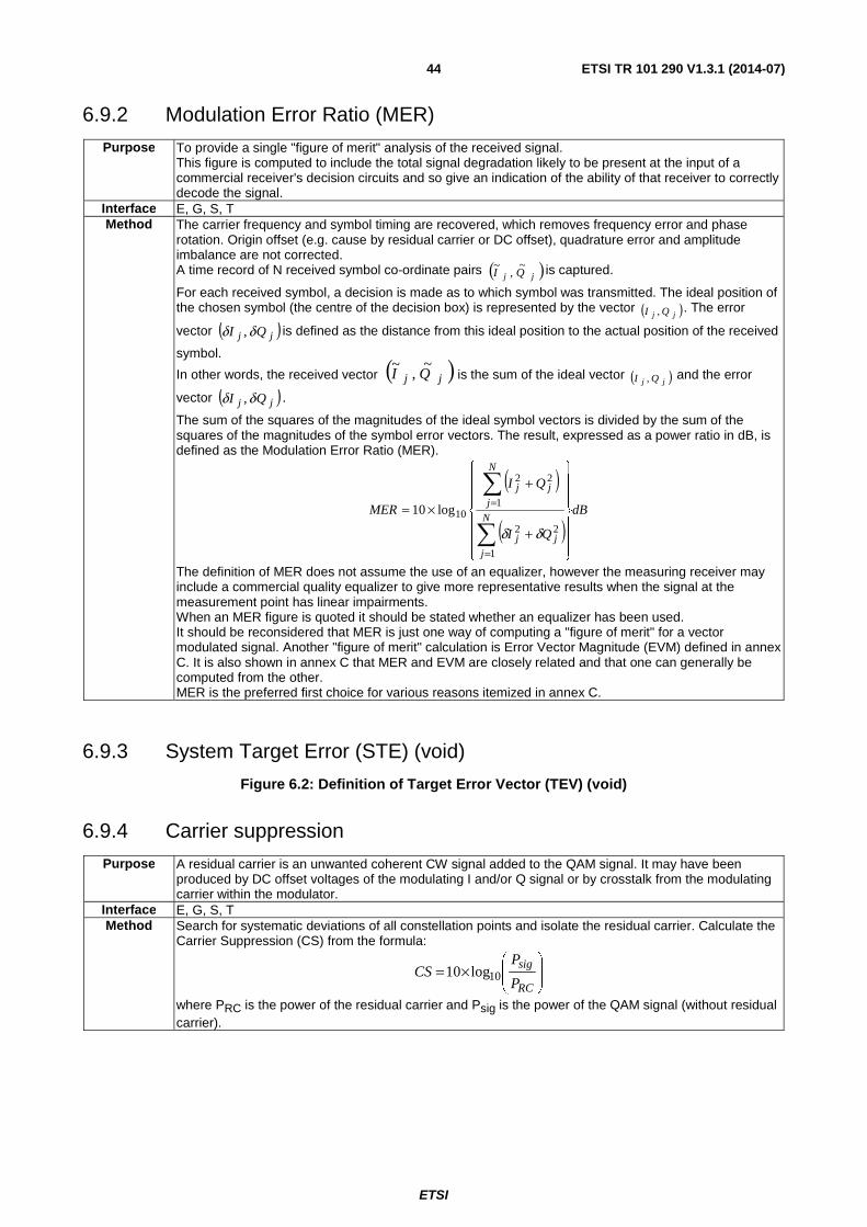
ETSI
ETSI TR 101 290 V1.3.1 (2014-07) 44
6.9.2 Modulation Error Ratio (MER)
Purpose To provide a single "figure of merit" analysis of the received signal. This figure is computed to include the total signal degradation likely to be present at the input of a commercial receiver's decision circuits and so give an indication of the ability of that receiver to correctly decode the signal.
Interface E, G, S, T Method The carrier frequency and symbol timing are recovered, which removes frequency error and phase
rotation. Origin offset (e.g. cause by residual carrier or DC offset), quadrature error and amplitude imbalance are not corrected. A time record of N received symbol co-ordinate pairs ( )jj QI
~,
~ is captured.
For each received symbol, a decision is made as to which symbol was transmitted. The ideal position of the chosen symbol (the centre of the decision box) is represented by the vector ( )jj QI , . The error
vector ( )jj QI δδ , is defined as the distance from this ideal position to the actual position of the received
symbol.
In other words, the received vector ( )jj QI~
,~
is the sum of the ideal vector ( )jj QI , and the error
vector ( )jj QI δδ , .
The sum of the squares of the magnitudes of the ideal symbol vectors is divided by the sum of the squares of the magnitudes of the symbol error vectors. The result, expressed as a power ratio in dB, is defined as the Modulation Error Ratio (MER).
( )
( )dB
QI
QI
MERN
j
jj
N
j
jj
⎪⎪⎪
⎭
⎪⎪⎪
⎬
⎫
⎪⎪⎪
⎩
⎪⎪⎪
⎨
⎧
+
+
×=
∑
∑
=
=
1
22
1
22
10log10
δδ
The definition of MER does not assume the use of an equalizer, however the measuring receiver may include a commercial quality equalizer to give more representative results when the signal at the measurement point has linear impairments. When an MER figure is quoted it should be stated whether an equalizer has been used. It should be reconsidered that MER is just one way of computing a "figure of merit" for a vector modulated signal. Another "figure of merit" calculation is Error Vector Magnitude (EVM) defined in annex C. It is also shown in annex C that MER and EVM are closely related and that one can generally be computed from the other. MER is the preferred first choice for various reasons itemized in annex C.
6.9.3 System Target Error (STE) (void)
Figure 6.2: Definition of Target Error Vector (TEV) (void)
6.9.4 Carrier suppression
Purpose A residual carrier is an unwanted coherent CW signal added to the QAM signal. It may have been produced by DC offset voltages of the modulating I and/or Q signal or by crosstalk from the modulating carrier within the modulator.
Interface E, G, S, T Method Search for systematic deviations of all constellation points and isolate the residual carrier. Calculate the
Carrier Suppression (CS) from the formula:
⎟⎟⎠
⎞⎜⎜⎝
⎛×=
RC
sig
P
PCS 10log10
where PRC is the power of the residual carrier and Psig is the power of the QAM signal (without residual carrier).

ETSI
ETSI TR 101 290 V1.3.1 (2014-07) 45
6.9.5 Amplitude Imbalance (AI)
Purpose To separate the QAM distortions resulting from AI of the I and Q signal from all other kind of distortions. Interface E, G, S, T Method Calculate the I and Q gain values vI and vQ from all points in a constellation diagram eliminating all
other influences. Calculate AI from νI and νQ:
. ),max( and ),min(
%1001
21
1
2
QIQI vvvvvvwith
v
vAI
==
×⎟⎟⎠
⎞⎜⎜⎝
⎛−=
( )
( )
( )
( )
( ) ( ) iQiIi
N
j
jQi
M
i i
QiiQ
N
j
jIi
M
i i
IiiI
ddd
QN
d
Q
dQ
M
IN
d
I
dI
M
=+
=
+=
=
+=
∑
∑
∑
∑
=
=
=
=
6.9.3) clause in given as id of component-(Q
6.9.3) clause in given as id of component-(I
1
1
1
1
1
1
1
1
δ
ν
δ
ν
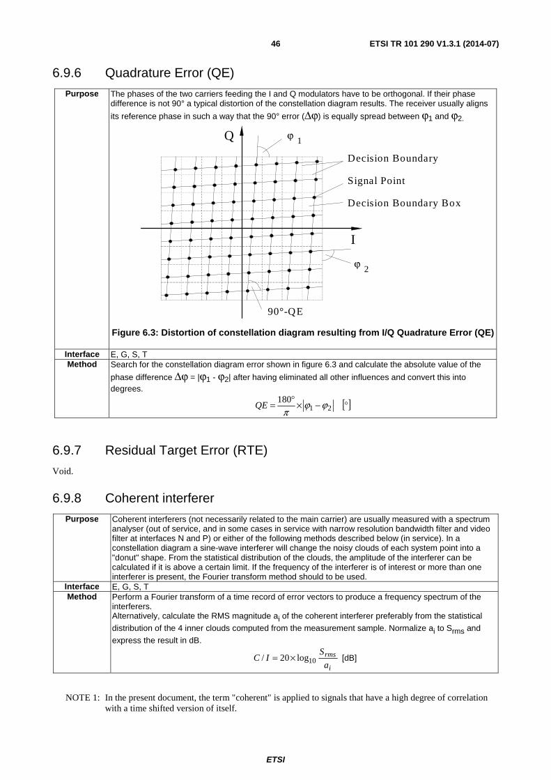
ETSI
ETSI TR 101 290 V1.3.1 (2014-07) 46
6.9.6 Quadrature Error (QE)
Purpose The phases of the two carriers feeding the I and Q modulators have to be orthogonal. If their phase difference is not 90° a typical distortion of the constellation diagram results. The receiver usually aligns
its reference phase in such a way that the 90° error (Δϕ) is equally spread between ϕ1 and ϕ2.
I
Q
Decision Boundary
Signal Point
Decision Boundary Box
1ϕ
2ϕ
90°-QE
Figure 6.3: Distortion of constellation diagram resulting from I/Q Quadrature Error (QE)
Interface E, G, S, T Method Search for the constellation diagram error shown in figure 6.3 and calculate the absolute value of the
phase difference Δϕ = |ϕ1 - ϕ2| after having eliminated all other influences and convert this into degrees.
[ ]°−×°= 21180 ϕϕ
πQE
6.9.7 Residual Target Error (RTE)
Void.
6.9.8 Coherent interferer
Purpose Coherent interferers (not necessarily related to the main carrier) are usually measured with a spectrum analyser (out of service, and in some cases in service with narrow resolution bandwidth filter and video filter at interfaces N and P) or either of the following methods described below (in service). In a constellation diagram a sine-wave interferer will change the noisy clouds of each system point into a "donut" shape. From the statistical distribution of the clouds, the amplitude of the interferer can be calculated if it is above a certain limit. If the frequency of the interferer is of interest or more than one interferer is present, the Fourier transform method should to be used.
Interface E, G, S, T Method Perform a Fourier transform of a time record of error vectors to produce a frequency spectrum of the
interferers. Alternatively, calculate the RMS magnitude ai of the coherent interferer preferably from the statistical
distribution of the 4 inner clouds computed from the measurement sample. Normalize ai to Srms and
express the result in dB.
i
rms
a
SIC 10log20/ ×= [dB]
NOTE 1: In the present document, the term "coherent" is applied to signals that have a high degree of correlation with a time shifted version of itself.
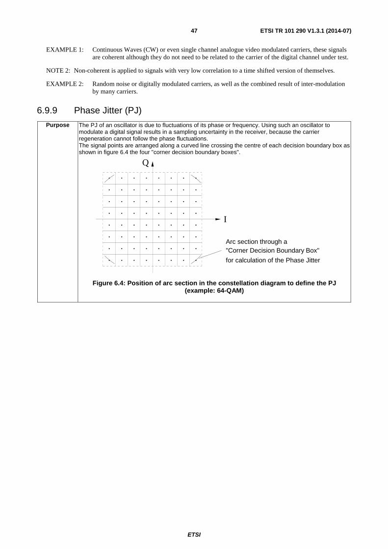
ETSI
ETSI TR 101 290 V1.3.1 (2014-07) 47
EXAMPLE 1: Continuous Waves (CW) or even single channel analogue video modulated carriers, these signals are coherent although they do not need to be related to the carrier of the digital channel under test.
NOTE 2: Non-coherent is applied to signals with very low correlation to a time shifted version of themselves.
EXAMPLE 2: Random noise or digitally modulated carriers, as well as the combined result of inter-modulation by many carriers.
6.9.9 Phase Jitter (PJ)
Purpose The PJ of an oscillator is due to fluctuations of its phase or frequency. Using such an oscillator to modulate a digital signal results in a sampling uncertainty in the receiver, because the carrier regeneration cannot follow the phase fluctuations. The signal points are arranged along a curved line crossing the centre of each decision boundary box as shown in figure 6.4 the four "corner decision boundary boxes".
Q
I
"Corner Decision Boundary Box"
for calculation of the Phase Jitter
Arc section through a
Figure 6.4: Position of arc section in the constellation diagram to define the PJ (example: 64-QAM)
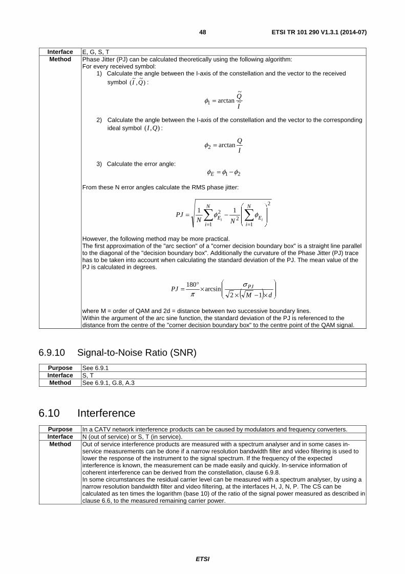
ETSI
ETSI TR 101 290 V1.3.1 (2014-07) 48
Interface E, G, S, T Method Phase Jitter (PJ) can be calculated theoretically using the following algorithm:
For every received symbol: 1) Calculate the angle between the I-axis of the constellation and the vector to the received
symbol )~
,~
( QI :
I
Q~
~arctan1 =φ
2) Calculate the angle between the I-axis of the constellation and the vector to the corresponding ideal symbol ),( QI :
I
Qarctan2 =φ
3) Calculate the error angle:
21 φφφ −=E
From these N error angles calculate the RMS phase jitter:
∑ ∑= =
⎟⎟
⎠
⎞
⎜⎜
⎝
⎛−=
N
i
N
iEE ii NN
PJ1
2
12
2 11 φφ
However, the following method may be more practical. The first approximation of the "arc section" of a "corner decision boundary box" is a straight line parallel to the diagonal of the "decision boundary box". Additionally the curvature of the Phase Jitter (PJ) trace has to be taken into account when calculating the standard deviation of the PJ. The mean value of the PJ is calculated in degrees.
( ) ⎟⎟
⎠
⎞
⎜⎜
⎝
⎛
×−××°=
dMPJ PJ
12arcsin
180 σπ
where M = order of QAM and 2d = distance between two successive boundary lines. Within the argument of the arc sine function, the standard deviation of the PJ is referenced to the distance from the centre of the "corner decision boundary box" to the centre point of the QAM signal.
6.9.10 Signal-to-Noise Ratio (SNR)
Purpose See 6.9.1 Interface S, T Method See 6.9.1, G.8, A.3
6.10 Interference Purpose In a CATV network interference products can be caused by modulators and frequency converters. Interface N (out of service) or S, T (in service). Method Out of service interference products are measured with a spectrum analyser and in some cases in-
service measurements can be done if a narrow resolution bandwidth filter and video filtering is used to lower the response of the instrument to the signal spectrum. If the frequency of the expected interference is known, the measurement can be made easily and quickly. In-service information of coherent interference can be derived from the constellation, clause 6.9.8. In some circumstances the residual carrier level can be measured with a spectrum analyser, by using a narrow resolution bandwidth filter and video filtering, at the interfaces H, J, N, P. The CS can be calculated as ten times the logarithm (base 10) of the ratio of the signal power measured as described in clause 6.6, to the measured remaining carrier power.
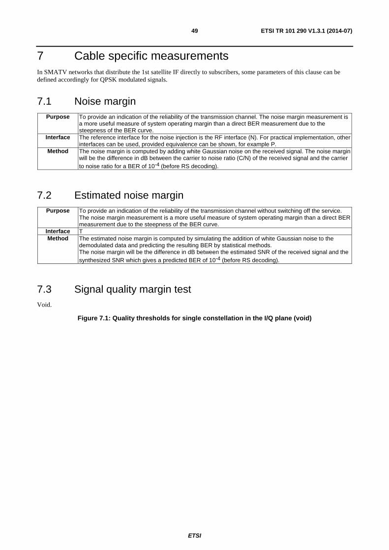
ETSI
ETSI TR 101 290 V1.3.1 (2014-07) 49
7 Cable specific measurements In SMATV networks that distribute the 1st satellite IF directly to subscribers, some parameters of this clause can be defined accordingly for QPSK modulated signals.
7.1 Noise margin Purpose To provide an indication of the reliability of the transmission channel. The noise margin measurement is
a more useful measure of system operating margin than a direct BER measurement due to the steepness of the BER curve.
Interface The reference interface for the noise injection is the RF interface (N). For practical implementation, other interfaces can be used, provided equivalence can be shown, for example P.
Method The noise margin is computed by adding white Gaussian noise on the received signal. The noise margin will be the difference in dB between the carrier to noise ratio (C/N) of the received signal and the carrier to noise ratio for a BER of 10-4 (before RS decoding).
7.2 Estimated noise margin Purpose To provide an indication of the reliability of the transmission channel without switching off the service.
The noise margin measurement is a more useful measure of system operating margin than a direct BER measurement due to the steepness of the BER curve.
Interface T Method The estimated noise margin is computed by simulating the addition of white Gaussian noise to the
demodulated data and predicting the resulting BER by statistical methods. The noise margin will be the difference in dB between the estimated SNR of the received signal and the synthesized SNR which gives a predicted BER of 10-4 (before RS decoding).
7.3 Signal quality margin test Void.
Figure 7.1: Quality thresholds for single constellation in the I/Q plane (void)
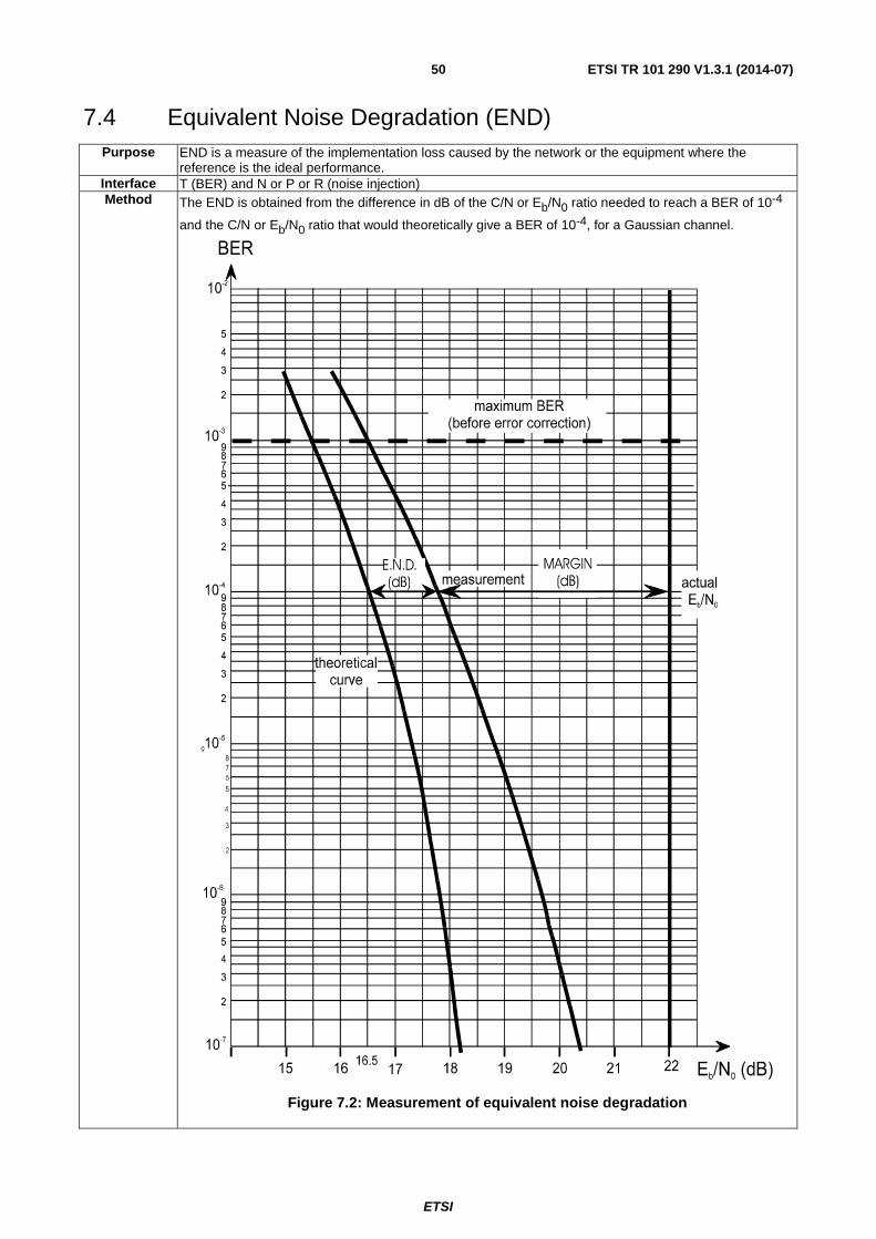
ETSI
ETSI TR 101 290 V1.3.1 (2014-07) 50
7.4 Equivalent Noise Degradation (END) Purpose END is a measure of the implementation loss caused by the network or the equipment where the
reference is the ideal performance. Interface T (BER) and N or P or R (noise injection) Method The END is obtained from the difference in dB of the C/N or Eb/N0 ratio needed to reach a BER of 10-4
and the C/N or Eb/N0 ratio that would theoretically give a BER of 10-4, for a Gaussian channel.
Figure 7.2: Measurement of equivalent noise degradation
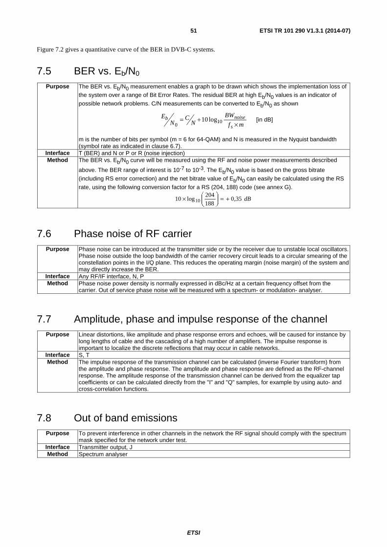
ETSI
ETSI TR 101 290 V1.3.1 (2014-07) 51
Figure 7.2 gives a quantitative curve of the BER in DVB-C systems.
7.5 BER vs. Eb/N0 Purpose The BER vs. Eb/N0 measurement enables a graph to be drawn which shows the implementation loss of
the system over a range of Bit Error Rates. The residual BER at high Eb/N0 values is an indicator of
possible network problems. C/N measurements can be converted to Eb/N0 as shown
mf
BWN
CN
E
s
noiseb×
+= 100
log10 [in dB]
m is the number of bits per symbol (m = 6 for 64-QAM) and N is measured in the Nyquist bandwidth (symbol rate as indicated in clause 6.7).
Interface T (BER) and N or P or R (noise injection) Method The BER vs. Eb/N0 curve will be measured using the RF and noise power measurements described
above. The BER range of interest is 10-7 to 10-3. The Eb/N0 value is based on the gross bitrate
(including RS error correction) and the net bitrate value of Eb/N0 can easily be calculated using the RS
rate, using the following conversion factor for a RS (204, 188) code (see annex G).
dB35,0188
204log10 10 +=⎟
⎠
⎞⎜⎝
⎛×
7.6 Phase noise of RF carrier Purpose Phase noise can be introduced at the transmitter side or by the receiver due to unstable local oscillators.
Phase noise outside the loop bandwidth of the carrier recovery circuit leads to a circular smearing of the constellation points in the I/Q plane. This reduces the operating margin (noise margin) of the system and may directly increase the BER.
Interface Any RF/IF interface, N, P Method Phase noise power density is normally expressed in dBc/Hz at a certain frequency offset from the
carrier. Out of service phase noise will be measured with a spectrum- or modulation- analyser.
7.7 Amplitude, phase and impulse response of the channel Purpose Linear distortions, like amplitude and phase response errors and echoes, will be caused for instance by
long lengths of cable and the cascading of a high number of amplifiers. The impulse response is important to localize the discrete reflections that may occur in cable networks.
Interface S, T Method The impulse response of the transmission channel can be calculated (inverse Fourier transform) from
the amplitude and phase response. The amplitude and phase response are defined as the RF-channel response. The amplitude response of the transmission channel can be derived from the equalizer tap coefficients or can be calculated directly from the "I" and "Q" samples, for example by using auto- and cross-correlation functions.
7.8 Out of band emissions Purpose To prevent interference in other channels in the network the RF signal should comply with the spectrum
mask specified for the network under test. Interface Transmitter output, J Method Spectrum analyser

ETSI
ETSI TR 101 290 V1.3.1 (2014-07) 52
8 Satellite specific measurements
8.1 BER before Viterbi decoding Purpose This measurement gives an indication of the transmission link performance. Due to typical error rates
ranging from 7 × 10⁻² to 10-5 the measurement can be done in a reasonable amount of time. Outside of this range the accuracy of the results may not be guaranteed.
Interface The measurement should be done before the Viterbi decoder (Interface T of the receiver). Method The signal after Viterbi decoding in the measurement instrument is coded again using the same coding
scheme as in the transmitter, in order to produce an estimate of the originally coded I and Q sequences. These sequences are compared at bit level with the sign-values of the signals that are available before Viterbi decoding. The BER for the I and Q paths should be made available separately. The measurement should be based on at least several hundred bit errors. For fast evaluation, in the case that the BER is lower than 10-4, it should be possible to stop the measurement after approximately 1 second. For accurate measurement of Eb/N0 at the quasi error free threshold, the measurement time and the
presentation of the result should be such that an accuracy of three decimal place can be achieved. The quasi error free threshold corresponds to a BER before Viterbi decoding in the range 7 × 10⁻² to 7 × 10⁻³,depending on the selected convolutional code rate; or a BER after Viterbi decoding of 2 × 10⁻⁴.
Figure 8.1: BER measurement before Viterbi decoding
8.2 Receive BER vs. Eb/N0 Purpose To verify overall clear sky link performance and link margin using a reference down link for acceptance
tests. Interface After Viterbi decoding, V Method This is an out-of-service-measurement. The BER measurement should be based on the null packets
inserted at the modulator as defined in clause A.1. To obtain the various values necessary for the curve BER over Eb/N0, white Gaussian noise is injected
at the receiver site. In order to get accurate results it should be verified that the inserted noise level is at least 15 dB above the system noise. This can easily be observed on a spectrum analyser by switching the inserted noise on and off. Stable reception conditions are a precondition for accurate measurement results. The RS decoding should be deactivated, or bypassed to avoid excessively long measurement periods. The BER range of interest is 10-9 to 10-2. The measurement values are compared with the theoretical values. The value for the Equivalent Noise Degradation (END) at a BER of 10-4 can be derived from this information as well. For evaluation of Eb/N0 only the number of information bits (the net bitrate) should be taken into
account.

ETSI
ETSI TR 101 290 V1.3.1 (2014-07) 53
8.3 IF spectrum Purpose To prevent interference into other channels and to be compliant with the DVB specification the
modulator output spectrum should be according with the one specified in EN 300 421 [i.5]. Interface H, input of the up-converter, typically 70 MHz or 140 MHz (Modulator output plus equipment for the
connection to the up-converter input). Method Spectrum analyser and template for amplitude response, network analyser and template for group delay
response, both as specified in EN 300 421 [i.5].
9 Measurements specific for a terrestrial (DVB-T) system
The intention of these guidelines is to provide a list of measurements useful in a DVB-T OFDM environment. The different options could be selected by the users of the system. Equipment manufacturers (both transmitters and receivers) as well as the operators, can choose those measurements that best fit their needs. A list of the applicability of the measurement parameters described in the present document to the DVB-T transmitter, receiver and network is given in table 9.1.
The measurements 6.1 "System availability" and 6.2 "Link availability" are also valid for Terrestrial (not only for Cable and Satellite) and for any contribution link like SDH, PDH, etc.
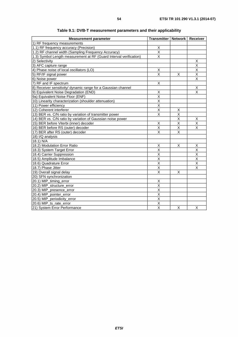
ETSI
ETSI TR 101 290 V1.3.1 (2014-07) 54
Table 9.1: DVB-T measurement parameters and their applicability
Measurement parameter Transmitter Network Receiver 1) RF frequency measurements 1.1) RF frequency accuracy (Precision) X 1.2) RF channel width (Sampling Frequency Accuracy) X 1.3) Symbol Length measurement at RF (Guard Interval verification) X 2) Selectivity X 3) AFC capture range X 4) Phase noise of local oscillators (LO) X X 5) RF/IF signal power X X X 6) Noise power X 7) RF and IF spectrum X 8) Receiver sensitivity/ dynamic range for a Gaussian channel X 9) Equivalent Noise Degradation (END) X X 9a) Equivalent Noise Floor (ENF) X 10) Linearity characterization (shoulder attenuation) X 11) Power efficiency X 12) Coherent interferer X X 13) BER vs. C/N ratio by variation of transmitter power X X 14) BER vs. C/N ratio by variation of Gaussian noise power X X 15) BER before Viterbi (inner) decoder X X X 16) BER before RS (outer) decoder X X X 17) BER after RS (outer) decoder X X 18) I/Q analysis 18.1) N/A 18.2) Modulation Error Ratio X X X 18.3) System Target Error X X 18.4) Carrier Suppression X X 18.5) Amplitude Imbalance X X 18.6) Quadrature Error X X 18.7) Phase Jitter X X 19) Overall signal delay X X 20) SFN synchronization 20.1) MIP_timing_error X 20.2) MIP_structure_error X 20.3) MIP_presence_error X 20.4) MIP_pointer_error X 20.5) MIP_periodicity_error X 20.6) MIP_ts_rate_error X 21) System Error Performance X X X
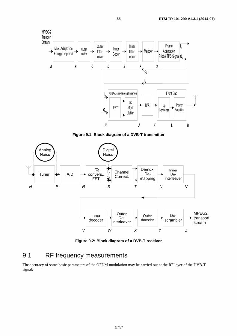
ETSI
ETSI TR 101 290 V1.3.1 (2014-07) 55
Figure 9.1: Block diagram of a DVB-T transmitter
Figure 9.2: Block diagram of a DVB-T receiver
9.1 RF frequency measurements The accuracy of some basic parameters of the OFDM modulation may be carried out at the RF layer of the DVB-T signal.
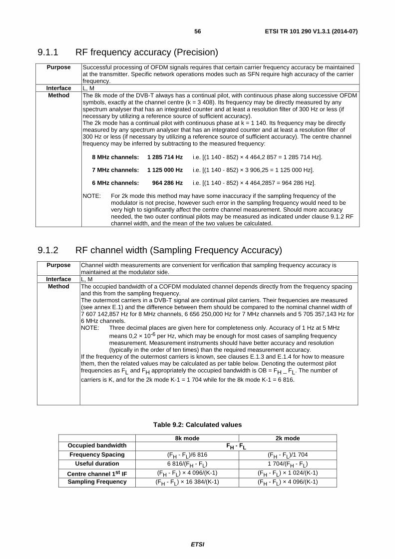
ETSI
ETSI TR 101 290 V1.3.1 (2014-07) 56
9.1.1 RF frequency accuracy (Precision)
Purpose Successful processing of OFDM signals requires that certain carrier frequency accuracy be maintained at the transmitter. Specific network operations modes such as SFN require high accuracy of the carrier frequency.
Interface L, M Method The 8k mode of the DVB-T always has a continual pilot, with continuous phase along successive OFDM
symbols, exactly at the channel centre (k = 3 408). Its frequency may be directly measured by any spectrum analyser that has an integrated counter and at least a resolution filter of 300 Hz or less (if necessary by utilizing a reference source of sufficient accuracy). The 2k mode has a continual pilot with continuous phase at k = 1 140. Its frequency may be directly measured by any spectrum analyser that has an integrated counter and at least a resolution filter of 300 Hz or less (if necessary by utilizing a reference source of sufficient accuracy). The centre channel frequency may be inferred by subtracting to the measured frequency:
8 MHz channels: 1 285 714 Hz i.e. [(1 140 - 852) × 4 464,2 857 = 1 285 714 Hz].
7 MHz channels: 1 125 000 Hz i.e. [(1 140 - 852) × 3 906,25 = 1 125 000 Hz].
6 MHz channels: 964 286 Hz i.e. [(1 140 - 852) × 4 464,2857 = 964 286 Hz].
NOTE: For 2k mode this method may have some inaccuracy if the sampling frequency of the modulator is not precise, however such error in the sampling frequency would need to be very high to significantly affect the centre channel measurement. Should more accuracy needed, the two outer continual pilots may be measured as indicated under clause 9.1.2 RF channel width, and the mean of the two values be calculated.
9.1.2 RF channel width (Sampling Frequency Accuracy)
Purpose Channel width measurements are convenient for verification that sampling frequency accuracy is maintained at the modulator side.
Interface L, M Method The occupied bandwidth of a COFDM modulated channel depends directly from the frequency spacing
and this from the sampling frequency. The outermost carriers in a DVB-T signal are continual pilot carriers. Their frequencies are measured (see annex E.1) and the difference between them should be compared to the nominal channel width of 7 607 142,857 Hz for 8 MHz channels, 6 656 250,000 Hz for 7 MHz channels and 5 705 357,143 Hz for 6 MHz channels. NOTE: Three decimal places are given here for completeness only. Accuracy of 1 Hz at 5 MHz
means 0,2 × 10⁻⁶ per Hz, which may be enough for most cases of sampling frequency measurement. Measurement instruments should have better accuracy and resolution (typically in the order of ten times) than the required measurement accuracy.
If the frequency of the outermost carriers is known, see clauses E.1.3 and E.1.4 for how to measure them, then the related values may be calculated as per table below. Denoting the outermost pilot frequencies as FL and FH appropriately the occupied bandwidth is OB = FH _ FL. The number of
carriers is K, and for the 2k mode K-1 = 1 704 while for the 8k mode K-1 = 6 816.
Table 9.2: Calculated values
8k mode 2k mode Occupied bandwidth FH - FL
Frequency Spacing (FH - FL)/6 816 (FH - FL)/1 704
Useful duration 6 816/(FH - FL) 1 704/(FH - FL)
Centre channel 1st IF (FH - FL) × 4 096/(K-1) (FH - FL) × 1 024/(K-1)
Sampling Frequency (FH - FL) × 16 384/(K-1) (FH - FL) × 4 096/(K-1)
ETSI
ETSI TR 101 290 V1.3.1 (2014-07) 57
9.1.3 Symbol Length measurement at RF (Guard Interval verification)
Purpose Verification of the guard interval used in a received DVB-T signal may be carried out at RF level by careful frequency measurements. This measurement is valid in cases where there is an uncertainty on whether a modulator is correctly working and producing a signal with the expected or assigned Guard Interval.
Interface L, M Method The scattered pilots produce a pulsed-like spectrum every third carrier in a DVB-T spectrum due to their
repetition presence at the same phase and location every fourth symbol. The frequency difference between two contiguous spectral lines representing a scattered pilot represents the inverse of the time length of four consecutive DVB-T symbols. Measuring such frequency difference and dividing its inverse by 4 will provide the total symbol length TS
of the measured signal. By subtracting the nominal useful symbol duration TU the length of the GI is
found. See clause E.1 for details on the measurement procedure and symbol lengths.
9.2 Selectivity Purpose To identify the capability of the receiver to reject out-of-channel interference. Interface The measurement of the signal input level and the interferer should be carried out at the interface N,
using interface W or X for the BER monitoring. Method The input power is adjusted to 10 dB above the minimum input power as defined in "Receiver
sensitivity" (see clause 9.8). The C/I threshold needed for QEF operation after RS decoder (BER < 2 x 10⁻⁴ before RS decoder) should be measured as a function of the frequency of a CW interferer.
9.3 AFC capture range Purpose To determine the frequency range over which the receiver will acquire overall lock. Interface N, for the application of the test signal; Z, for the test of TS synchronization Method A signal is applied to the input of the receiver, at a level 10 dB above the minimum input power as
defined in "Receiver sensitivity" (see clause 9.8). The signal is frequency shifted in steps (from below and above) towards a nominal value and the Sync_byte_error is verified according to clause 5.2.1 (Measurement and analysis of the MPEG-2 TS - First priority: necessary for decodability (basic monitoring)).
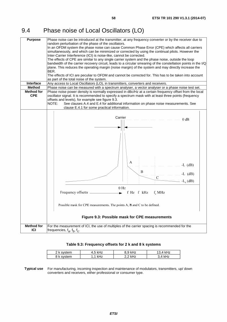
ETSI
ETSI TR 101 290 V1.3.1 (2014-07) 58
9.4 Phase noise of Local Oscillators (LO) Purpose Phase noise can be introduced at the transmitter, at any frequency converter or by the receiver due to
random perturbation of the phase of the oscillators. In an OFDM system the phase noise can cause Common Phase Error (CPE) which affects all carriers simultaneously, and which can be minimized or corrected by using the continual pilots. However the Inter-Carrier Interference (ICI) is noise-like, cannot be corrected. The effects of CPE are similar to any single carrier system and the phase noise, outside the loop bandwidth of the carrier recovery circuit, leads to a circular smearing of the constellation points in the I/Q plane. This reduces the operating margin (noise margin) of the system and may directly increase the BER. The effects of ICI are peculiar to OFDM and cannot be corrected for. This has to be taken into account as part of the total noise of the system.
Interface Any access to Local Oscillators (LO), in transmitters, converters and receivers. Method Phase noise can be measured with a spectrum analyser, a vector analyser or a phase noise test set.
Method for CPE
Phase noise power density is normally expressed in dBc/Hz at a certain frequency offset from the local oscillator signal. It is recommended to specify a spectrum mask with at least three points (frequency offsets and levels), for example see figure 9.3. NOTE: See clauses A.4 and E.4 for additional information on phase noise measurements. See
clause E.4.1 for some practical information.
Carrier
Figure 9.3: Possible mask for CPE measurements
Method for ICI
For the measurement of ICI, the use of multiples of the carrier spacing is recommended for the frequencies, fa, fb, fc.
Table 9.3: Frequency offsets for 2 k and 8 k systems
2 k system 4,5 kHz 8,9 kHz 13,4 kHz 8 k system 1,1 kHz 2,2 kHz 3,4 kHz
Typical use For manufacturing, incoming inspection and maintenance of modulators, transmitters, up/ down converters and receivers, either professional or consumer type.
ETSI
ETSI TR 101 290 V1.3.1 (2014-07) 59
9.5 RF/IF signal power Purpose Signal power, or wanted power, measurement is required to set and check signal levels at the
transmitter and receiver sites. Interface K, L, M, N, P Method The signal power of a terrestrial DVB signal, or wanted power, is defined as the mean power of the
signal as would be measured with a thermal power sensor. In the case of received signals care should be taken to limit the measurement to the bandwidth at the wanted signal. When using a spectrum analyser or a calibrated receiver, it should integrate the signal power within the nominal bandwidth of the signal (n × fSPACING) where n is the number of carriers.
9.6 Noise power Purpose Noise is a significant impairment in a transmission network. Interface N,P Method The noise power (mean power), or unwanted power, can be measured with a spectrum analyser (out of
service). The noise power is specified using the occupied bandwidth of the OFDM signal (n × fSPACING) where n is the number of carriers.
NOTE: The term C/N should be calculated as the ratio of the signal power, measured as described in clause 9.5, to the noise power, measured as described in this clause.
9.7 RF and IF spectrum Purpose To avoid interfering with other channels, the transmitted RF spectrum should comply with a spectrum
mask, which is defined for the terrestrial network. If the spectrum at the modulator output is defined by a spectrum mask, the same procedure can be applied to the IF signal (with no pre-correction active).
Interface K, M Method This measurement is usually carried out using a spectrum analyser. The spectral density of a terrestrial
DVB signal is defined as the long-term average of the time-varying signal power per unity bandwidth (i.e. 1 Hz). Values for other bandwidths can be achieved by proportional increase of the values for unity bandwidth. To avoid regular structures in the modulated signal a non-regular, e.g. a Pseudo-Random Binary Sequence (PRBS) -like or a programme type digital transmitter input signal is necessary. Care has to be taken that the input stage of the selective measurement equipment is not overloaded by the main lobe of the signal while assessing the spectral density of the side lobes, i. e. the out-of-band range. Especially in cases with very strong attenuation of the side lobes non-linear distortion in the measurement equipment can produce side lobe signals that mask the original ones. Selective attenuation of the main lobe has proven to be in principal a way to avoid this masking effects. However, as the frequency response of the band-stop filter has to be included in the evaluation, the whole measurement procedure may become somewhat complex. For the resolution bandwidth, the recommended values should not exceed 30 kHz. Preferred values are approximately 4 kHz. The measurement should be Noise-normalized to 4 kHz.
9.8 Receiver sensitivity/ dynamic range for a Gaussian channel Purpose For network planning purposes, the minimum and maximum input powers for normal operation of a
receiver have to be determined. Interface Test signals are applied and measured at interface N; interfaces W or X are used for the monitoring of
BER before RS. Method The minimum and maximum input power thresholds for QEF (Quasi Error Free) operation after the RS
decoder (i.e. BER < 2 × 10⁻⁴ before RS decoding) should be measured. The dynamic range is the difference between the measured values.
ETSI
ETSI TR 101 290 V1.3.1 (2014-07) 60
9.9 Equivalent Noise Degradation (END) Purpose END is a measure of the implementation loss caused by the network or the equipment where the
reference is the ideal performance. Interface W or X for BER measurement; N, P or S for noise injection Method The END is obtained from the difference in dB of the C/N ratio needed to reach a BER of 2 × 10⁻⁴ before
RS (outer) decoding, and the C/N ratio that would theoretically give a BER of 2 × 10⁻⁴ for a Gaussian channel (see annex A of EN 300 744 [i.9]).
9.9.1 Equivalent Noise Floor (ENF)
Purpose ENF is a measure of the implementation loss caused by the transmitting equipment where the reference is the ideal transmitter.
Interface M for noise power measurement, W or X for BER measurement; N, P or S for noise injection Method The ENF is obtained from the measurement of additional noise needed to reach a BER of 2 × 10⁻⁴
before RS (outer) decoding, and the noise level that would theoretically give a BER of 2 × 10⁻⁴ for a Gaussian channel (see annex A of EN 300 744 [i.9]) as described in clause B.12.
Note on END and ENF:
The impact of the DVB-T transmitter on the overall system performance, when a certain DVB-T mode is being received by the reference receiver, via a Gaussian channel, is assessed by the measurement of the END.
The reference receiver is in the present document defined as a DVB-T receiver which require a C/N which is 3,0 dB higher than the C/N figures indicated in EN 300 744 [i.9], on a Gaussian channel.
The END is in the present document defined to be the difference between required C/N, for a BER of 2 × 10⁻⁴ after convolutional decoding on the reference receiver, using a real and an ideal DVB-T transmitter.
The END is not only a characteristic of the transmitter itself but is also dependent on the used DVB-T mode and on the receiver implementation loss (this is why a fixed 3,0 dB receiver implementation loss is defined for the reference receiver).
The END should not exceed [0,5] dB and should be independent of the selected guard interval. Depending on the requirements of the network operator typical END values fall in the range [0,1-0,4] dB.
For the determination of the END value another parameter, the Equivalent Noise Floor ENF, can be used. As described in clause B.12, this should result in an improved accuracy for the END.
As opposed to the END the ENF is relatively independent of the DVB-T mode used and on the receiver implementation loss and can therefore be used to characterize the transmitter by itself. Depending on whether there is a need for characterizing the DVB-T transmitter by itself, or whether there is a need to characterize its effect on a receiver, the ENF can sometimes be used as an alternative to END as a performance parameter.
The influences of intermodulation and amplitude ripple are expected to dominate in practise in the performance parameter END.
(The Group Delay response of a transmitter needs to be defined by network operators depending on the configuration in use (channel combiners, output filters, etc.).)
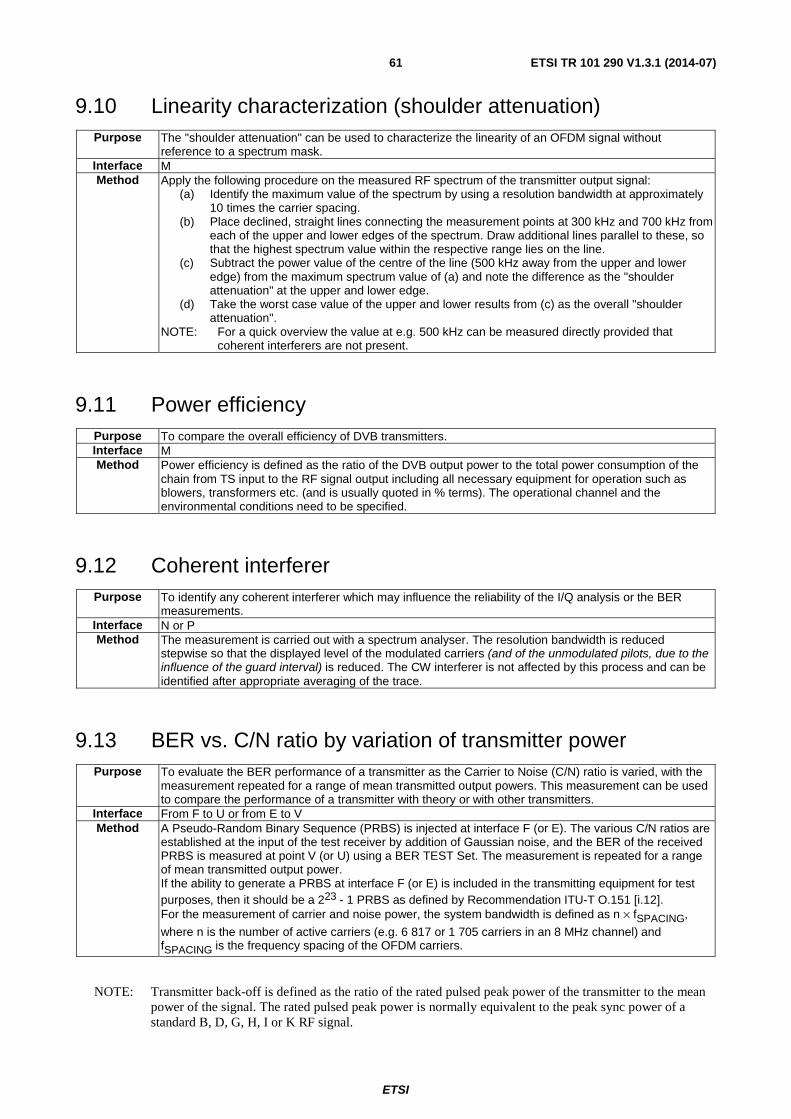
ETSI
ETSI TR 101 290 V1.3.1 (2014-07) 61
9.10 Linearity characterization (shoulder attenuation) Purpose The "shoulder attenuation" can be used to characterize the linearity of an OFDM signal without
reference to a spectrum mask. Interface M Method Apply the following procedure on the measured RF spectrum of the transmitter output signal:
(a) Identify the maximum value of the spectrum by using a resolution bandwidth at approximately 10 times the carrier spacing.
(b) Place declined, straight lines connecting the measurement points at 300 kHz and 700 kHz from each of the upper and lower edges of the spectrum. Draw additional lines parallel to these, so that the highest spectrum value within the respective range lies on the line.
(c) Subtract the power value of the centre of the line (500 kHz away from the upper and lower edge) from the maximum spectrum value of (a) and note the difference as the "shoulder attenuation" at the upper and lower edge.
(d) Take the worst case value of the upper and lower results from (c) as the overall "shoulder attenuation".
NOTE: For a quick overview the value at e.g. 500 kHz can be measured directly provided that coherent interferers are not present.
9.11 Power efficiency Purpose To compare the overall efficiency of DVB transmitters. Interface M Method Power efficiency is defined as the ratio of the DVB output power to the total power consumption of the
chain from TS input to the RF signal output including all necessary equipment for operation such as blowers, transformers etc. (and is usually quoted in % terms). The operational channel and the environmental conditions need to be specified.
9.12 Coherent interferer Purpose To identify any coherent interferer which may influence the reliability of the I/Q analysis or the BER
measurements. Interface N or P Method The measurement is carried out with a spectrum analyser. The resolution bandwidth is reduced
stepwise so that the displayed level of the modulated carriers (and of the unmodulated pilots, due to the influence of the guard interval) is reduced. The CW interferer is not affected by this process and can be identified after appropriate averaging of the trace.
9.13 BER vs. C/N ratio by variation of transmitter power Purpose To evaluate the BER performance of a transmitter as the Carrier to Noise (C/N) ratio is varied, with the
measurement repeated for a range of mean transmitted output powers. This measurement can be used to compare the performance of a transmitter with theory or with other transmitters.
Interface From F to U or from E to V Method A Pseudo-Random Binary Sequence (PRBS) is injected at interface F (or E). The various C/N ratios are
established at the input of the test receiver by addition of Gaussian noise, and the BER of the received PRBS is measured at point V (or U) using a BER TEST Set. The measurement is repeated for a range of mean transmitted output power. If the ability to generate a PRBS at interface F (or E) is included in the transmitting equipment for test purposes, then it should be a 223 - 1 PRBS as defined by Recommendation ITU-T O.151 [i.12]. For the measurement of carrier and noise power, the system bandwidth is defined as n × fSPACING,
where n is the number of active carriers (e.g. 6 817 or 1 705 carriers in an 8 MHz channel) and fSPACING is the frequency spacing of the OFDM carriers.
NOTE: Transmitter back-off is defined as the ratio of the rated pulsed peak power of the transmitter to the mean power of the signal. The rated pulsed peak power is normally equivalent to the peak sync power of a standard B, D, G, H, I or K RF signal.

ETSI
ETSI TR 101 290 V1.3.1 (2014-07) 62
9.14 BER vs. C/N ratio by variation of Gaussian noise power Purpose To evaluate the BER performance of a receiver as the Carrier to Noise (C/N) ratio is varied by changing
the added Gaussian noise power. This measurement can be used to compare the performance of a receiver with theory or with other receivers. For example to evaluate the influence of receiver noise floor.
Interface From F to U or from E to V. Method A Pseudo-Random Binary Sequence (PRBS) is injected at interface F (or E). Various C/N ratios are
established at the input of the receiver under test by addition of Gaussian noise and the BER of the received PRBS is measured at point V (or U) using a BER test set. A test transmitter should be able to generate the 223 - 1 PRBS as defined by Recommendation ITU-T O.151 [i.12]. For the measurement of carrier and noise power, the system bandwidth is defined as n × fSPACING
where n is the number of active carriers i. e. 6 817 or 1 705 carriers and fSPACING is the frequency
spacing of the OFDM carriers.
NOTE: The bandwidth in an 8 MHz channel is approx. 7,61 MHz, in a 7 MHz channel system it is 6,66 MHz and 5,71 MHz in a 6 MHz channel.
9.15 BER before Viterbi (inner) decoder Purpose This measurement gives an in-service indication of the un-coded performance of the transmitter,
channel and receiver. Interface V. Method The signal after Viterbi decoding in the test receiver is coded again using the same convolutional coding
scheme as in the transmitter in order to produce an estimate of the originally coded data stream. This data stream is compared at bit-level with the signal which is available before Viterbi decoder. The measurement should be based on at least several hundred bit errors.
Viterbi Decoder
Delay
ConvolutionalCoder
Outerde-interleaver
Comparison
BER
V W X
Figure 9.4: BER measurement before Viterbi decoding
9.16 BER before RS (outer) decoder Purpose The BER is the primary parameter which describes the quality of the digital transmission link. Interface W or X Method The BER is defined as the ratio between erroneous bits and the total number of transmitted bits.
Two alternative methods are available; one for "Out of Service" and a second for "In Service" use. In both cases, the measurement should only be done within the Link Available Time (LAT) as defined in clause 6.2.
9.16.1 Out of Service
The basic principle of this measurement is to generate within the channel encoder a known, fixed, repeating sequence of bits, essentially of a Pseudo-Random nature. In order to do this the data entering the sync-inversion/randomization function is a continuous repetition of one fixed TS packet. This sequence is defined as the null TS packet in ISO/IEC 13818-1 [i.1] with all data bytes set to 0x00; i.e. the fixed packet is defined as the four byte sequence 0x47, 0x1F, 0xFF, 0x10, followed by 184 zero bytes (0x00). Ideally this would be available as an encoding system option.
ETSI
ETSI TR 101 290 V1.3.1 (2014-07) 63
The apparently obvious alternative of injecting a PRBS in the transmitter at the output of the RS encoder is not used because of the requirement to have sync bytes to ensure correct operation of the byte interleaver. Insertion after the byte interleaver is not appropriate because it is not then directly comparable with the in-service measurement.
9.16.2 In Service
The basic assumption made in this measurement method is that the RS check bytes are computed for each link in the transmission chain. Under normal operational circumstances, the RS decoder will correct all errors and produce an error-free TS packet. If there are severe error-bursts, the RS decoding algorithm may be overloaded, and be unable to correct the packet. In this case the transport_error_indicator bit should be set, no other bits in the packet should be changed, and the 16 RS check bytes should be recalculated accordingly before re-transmission on to another link. The BER measured at any point in the transmission chain is then the BER for that particular link only.
The number of erroneous bits within a TS packet will be estimated by comparing the bit pattern of this TS packet before and after RS decoding. If the measured value of BER exceeds 10-3 then the measurement should be regarded as unreliable due to the limits of the RS decoding algorithm. Any TS packet that the RS decoder is unable to correct should cause the calculation to be restarted.
9.17 BER after RS (outer) decoder (Bit error count) Purpose To gain information about the pattern with which bit errors occur. Interface Z Method The same principle as used for the "Out of service" measurement of the "BER before the RS decoder"
described in clause 9.16.1, with the modification that the result is presented as an error count rather than a ratio. The receiver only has to compare the received TS packets with the Null packets as defined in clause A.1.2. This method is applicable for cases where the BER before RS decoder is lower than approximatively 10-3. This can be used as one parameter for the estimation of the quality of the transmission link as it was defined by the operator, or for localization of specific problems.
9.18 IQ signal analysis
9.18.1 Introduction
The IQ analysis can be applied on single carriers of the OFDM signal as well as on groups of carriers. If groups of carriers are under consideration all received symbols of this group can be superimposed in order to get one common constellation diagram. Since the scattered pilot carriers, the continual pilot carriers and the TPS carriers are transmitted in a different modulation scheme it is recommended to exclude these carriers from the IQ analysis or apply a specific IQ analysis.
Assuming:
- a constellation diagram of M symbol points and K carriers under consideration with 0 < K ≤ KMAX +1 and KMAX + 1 is the total number of active OFDM carriers (i.e. 1 705 or 6 817 carriers);
- a measurement sample of N data points, where N is sufficiently larger than M × K to deliver the wanted measurement accuracy; and
- the co-ordinates of each received data point j being Ij + δIj, Qj + δQj where I and Q are the co-ordinates of the
ideal symbol point and δI and δQ are the offsets forming the error vector of the data point (as long as the respective carrier is a "useful" one).
The following six parameters can be calculated, which give an in-depth analysis of different influences, all deteriorating the signal.
Modulation Error Ratio (MER) and the related Error Vector Magnitude (EVM) are calculated from all N data points without special pre-calculation for the data belonging to the M symbol points.

ETSI
ETSI TR 101 290 V1.3.1 (2014-07) 64
With the aim of separating individual influences from the received data, for each point i of the M symbol points the mean distance di and the distribution σi can be calculated from those δIj, δQj belonging to the point i.
From the M values {d1, d2, ... dM} the influences/ parameters:
- Origin offset/ Carrier suppression (CS);
- Amplitude Imbalance; and
- Quadrature Error (QE)
(only for 2 k modes since the centre carrier needs to carry a complete constellation which is not the case in an 8k system where the centre carrier is a continual pilot) can be extracted and removed from the di values, allowing to calculate the
Residual Target Error (RTE) with the same algorithm as the System Target Error (STE) from {d1, d2, ... dM}.
From the statistical distribution of the M clouds the parameters:
- Phase Jitter (PJ); and
- coherent interferer (if it is dominant)
may be extracted. The remaining clouds (after elimination of the above two influences) are assumed to be due to Gaussian noise only and are the basis for calculation of the signal-to-noise ratio. The parameter may include - besides noise - also some other disturbing effects, like small coherent interferers or residual errors from the channel correction.
When using the interfaces S or T filtering of the signal before the interface should be considered.
The parameters Origin offset/ Carrier suppression (CS), Amplitude Imbalance (AI) and Quadrature Error (QE) are typical performance parameters of the modulator. The other parameters are also influenced by the transmission system and the receiver/ demodulator.
It should be noted that the channel estimation/ channel correction mechanism can have an impact on the measurement results. This is particularly true for measurements in the field or under simulated but realistic reception conditions.
For measurements taken at the output of a transmitter this impact of the channel estimation/ channel correction mechanism is negligible.
For comparison of measurement results, information on the character of the channel estimation/ channel correction mechanism should be provided.
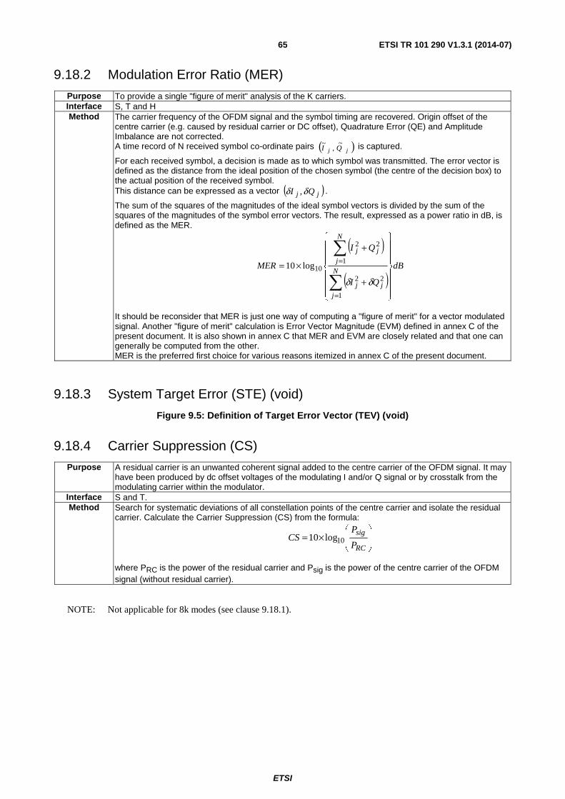
ETSI
ETSI TR 101 290 V1.3.1 (2014-07) 65
9.18.2 Modulation Error Ratio (MER)
Purpose To provide a single "figure of merit" analysis of the K carriers. Interface S, T and H Method The carrier frequency of the OFDM signal and the symbol timing are recovered. Origin offset of the
centre carrier (e.g. caused by residual carrier or DC offset), Quadrature Error (QE) and Amplitude Imbalance are not corrected. A time record of N received symbol co-ordinate pairs ( )jj QI
~,
~ is captured.
For each received symbol, a decision is made as to which symbol was transmitted. The error vector is defined as the distance from the ideal position of the chosen symbol (the centre of the decision box) to the actual position of the received symbol. This distance can be expressed as a vector ( )jj QI δδ , .
The sum of the squares of the magnitudes of the ideal symbol vectors is divided by the sum of the squares of the magnitudes of the symbol error vectors. The result, expressed as a power ratio in dB, is defined as the MER.
( )
( )dB
QI
QI
MERN
j
jj
N
j
jj
⎪⎪⎪
⎭
⎪⎪⎪
⎬
⎫
⎪⎪⎪
⎩
⎪⎪⎪
⎨
⎧
+
+
×=
∑
∑
=
=
1
22
1
22
10log10
δδ
It should be reconsider that MER is just one way of computing a "figure of merit" for a vector modulated signal. Another "figure of merit" calculation is Error Vector Magnitude (EVM) defined in annex C of the present document. It is also shown in annex C that MER and EVM are closely related and that one can generally be computed from the other. MER is the preferred first choice for various reasons itemized in annex C of the present document.
9.18.3 System Target Error (STE) (void)
Figure 9.5: Definition of Target Error Vector (TEV) (void)
9.18.4 Carrier Suppression (CS)
Purpose A residual carrier is an unwanted coherent signal added to the centre carrier of the OFDM signal. It may have been produced by dc offset voltages of the modulating I and/or Q signal or by crosstalk from the modulating carrier within the modulator.
Interface S and T. Method Search for systematic deviations of all constellation points of the centre carrier and isolate the residual
carrier. Calculate the Carrier Suppression (CS) from the formula:
⎟⎟⎠
⎞⎜⎜⎝
⎛×=
RC
sig
P
PCS 10log10
where PRC is the power of the residual carrier and Psig is the power of the centre carrier of the OFDM signal (without residual carrier).
NOTE: Not applicable for 8k modes (see clause 9.18.1).
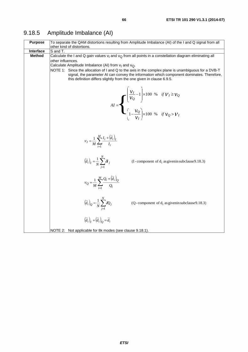
ETSI
ETSI TR 101 290 V1.3.1 (2014-07) 66
9.18.5 Amplitude Imbalance (AI)
Purpose To separate the QAM distortions resulting from Amplitude Imbalance (AI) of the I and Q signal from all other kind of distortions.
Interface S and T. Method Calculate the I and Q gain values vI and vQ from all points in a constellation diagram eliminating all
other influences. Calculate Amplitude Imbalance (AI) from vI and vQ. NOTE 1: Since the allocation of I and Q to the axis in the complex plane is unambiguous for a DVB-T
signal, the parameter AI can convey the information which component dominates. Therefore, this definition differs slightly from the one given in clause 6.9.5.
ν
ν
IQI
Q
QIQ
I
vvv
vvv
if
if
AI
>×⎟⎟⎠
⎞⎜⎜⎝
⎛−
≥×⎟⎟⎟
⎠
⎞
⎜⎜⎜
⎝
⎛−
=
%1001
%1001
{
( )
( )
( )
( )
( ) ( ) iQiIi
N
j
jQi
M
i i
QiiQ
N
j
jIi
M
i i
IiiI
ddd
QN
d
Q
dQ
M
IN
d
I
dI
M
=+
=
+=
=
+=
∑
∑
∑
∑
=
=
=
=
9.18.3) subclausein given as d ofcomponent -(Q 1
1
9.18.3) subclausein given as d ofcomponent-(I 1
1
i
1
1
i
1
1
δ
ν
δ
ν
NOTE 2: Not applicable for 8k modes (see clause 9.18.1).
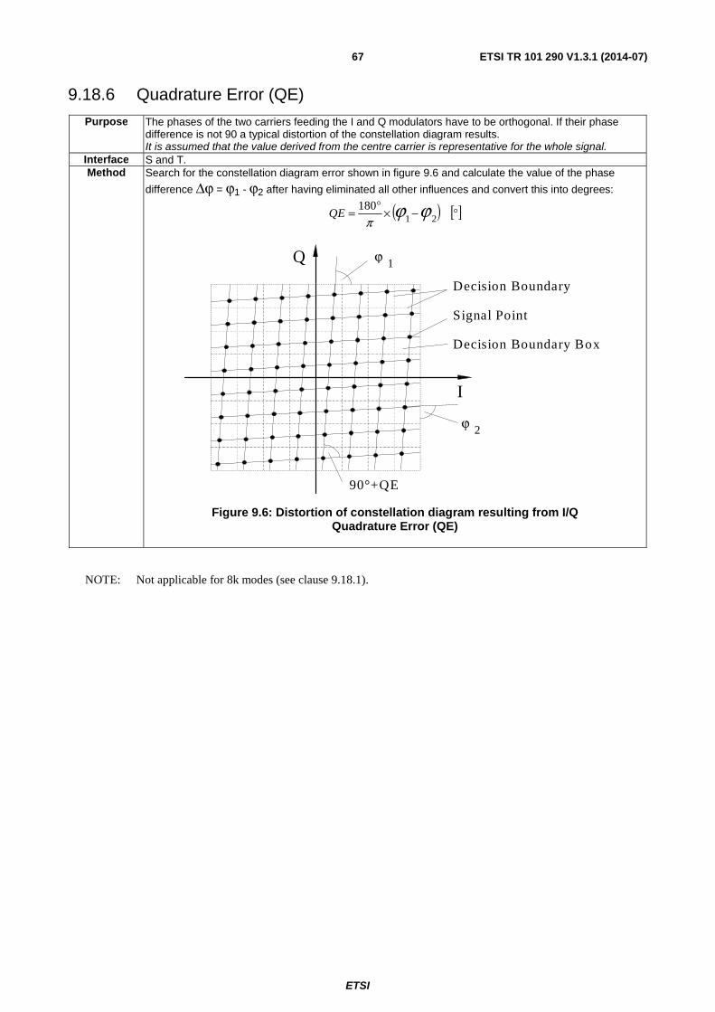
ETSI
ETSI TR 101 290 V1.3.1 (2014-07) 67
9.18.6 Quadrature Error (QE)
Purpose The phases of the two carriers feeding the I and Q modulators have to be orthogonal. If their phase difference is not 90 a typical distortion of the constellation diagram results. It is assumed that the value derived from the centre carrier is representative for the whole signal.
Interface S and T. Method Search for the constellation diagram error shown in figure 9.6 and calculate the value of the phase
difference Δϕ = ϕ1 - ϕ2 after having eliminated all other influences and convert this into degrees:
( ) [ ]°−×°= ϕϕπ 21
180QE
I
Q
Decision Boundary
Signal Point
Decision Boundary Box
1ϕ
2ϕ
90°+QE
Figure 9.6: Distortion of constellation diagram resulting from I/Q Quadrature Error (QE)
NOTE: Not applicable for 8k modes (see clause 9.18.1).

ETSI
ETSI TR 101 290 V1.3.1 (2014-07) 68
9.18.7 Phase Jitter (PJ)
Purpose The PJ of an oscillator is due to fluctuations of its phase or frequency. Using such an oscillator to modulate a digital signal results in a sampling uncertainty in the receiver, because the carrier regeneration cannot follow the phase fluctuations. The signal points are arranged along a curved line crossing the centre of each decision boundary box as shown in figure 9.7 for the four "Corner Decision Boundary Boxes".
Q
I
"Corner Decision Boundary Box"
for calculation of the Phase Jitter
Arc section through a
Figure 9.7: Position of "Arc section" in the constellation diagram to define PJ (example: 64-QAM)
Interface S and T. Method Phase Jitter can be calculated theoretically using the following algorithm:
1) Calculate the angle between the I-axis of the constellation and the vector to the received symbol ),( rcvdrcvd QI :
rcvd
rcvd
I
Qarctan1 =φ
2) Calculate the angle between the I-axis of the constellation and the vector to the corresponding ideal symbol ),( idealideal QI :
ideal
ideal
I
Qarctan2 =φ
Phi 2 instead of Phi 1 3) Calculate the error angle:
21 φφφ −=E
4) From these N error angles calculate the RMS phase jitter:
∑ ∑= =
⎟⎟
⎠
⎞
⎜⎜
⎝
⎛−=
N
i
N
iEE ii NN
PJ1
2
12
2 11 φφ
However, the following method may be more practical: The first approximation of the "Arc Section" of a "Corner Decision Boundary Box" is a straight line parallel to the diagonal of the "Decision Boundary Box". Additionally the curvature of the Phase Jitter (PJ) trace has to be taken into account when calculating the standard deviation of the PJ. The mean value of the PJ is calculated in degrees.
( ) ⎟⎟
⎠
⎞
⎜⎜
⎝
⎛
×−××°=
dMPJ PJ
12arcsin
180 σπ
[°]
where M = Order of QAM and 2d = Distance between two successive boundary lines Within the argument of the arc sine function, the standard deviation of the Phase Jitter is referenced to the distance from the centre of the "Corner Decision Boundary Box" to the centre point of the QAM signal.
ETSI
ETSI TR 101 290 V1.3.1 (2014-07) 69
9.19 Overall signal delay Purpose To measure and adjust the signal delay of an OFDM transmitter to a given value so that the transmitters
in an SFN can be synchronized. Interface A, M. Method (a) The total delay between the MPEG TS input of the transmitter under test and the MPEG TS
output of a test receiver is established by measuring the time delay required to match the input and output data patterns. If the delay of the test receiver is known then the transmitter signal delay can be derived.
Alternatively, the delay of the test receiver could be expressed relative to the delay of a reference receiver. This would avoid the need to measure the absolute delay of any receiver.
(b) A more direct method may be to define a transmitter test mode in which the occurrence of a Mega-frame Initialization Packet (MIP) at the MPEG TS input causes a trigger pulse (see TS 101 191 [i.14]).
The trigger pulse is made available for connection to an oscilloscope and also used to "arm" the modulator. At the start of the next mega-frame the modulator transmits a null symbol (or a defined pulse in the time domain) rather than the normal data. The delay between the trigger pulse and the RF null (or pulse) is measured.
(c) The delay of a transmitter could be expressed relative to the delay of a reference transmitter. For the measurement a reduced amplitude sample is taken from both transmitters and adjusted to have similar level (< 3 dB difference), the samples are combined in a RF linear adder and the output is fed to a spectrum analyser. Typically the spectrum formed will have lobes due to the difference of delays in the two transmitters. The inverse of the frequency width of the lobes represents the relative delay between the transmitters.
Two drawbacks has to be taken in account: 1) the delay is absolute, that is, it gives no indication of which transmitter has the longer delay; 2) the accuracy is related to the ability of identifying the minimal values of the lobes and the
accuracy of the measurement. NOTE 1: The delay of a transmitter may be considered as the addition of various parts including the
physical delays of the analogue part of the OFDM signal, including the path length to the antenna. Also the buffers used for signal conditioning (TS bitrate adaptation to the sampling frequency of the transmitter) and other intermediate buffers in the OFDM spectrum calculation (IFFT) may differ from manufacturer to manufacturer.
NOTE 2: In cases of single frequency networks, the SFN adapter at the transmitter site may be considered as integral part of the modulator transmitter. It may calculate the delay, from the value of the STS (Synchronization Time Stamp) to the 1 pps used as reference, in different way from manufacturer to manufacturer and add differences in the delays that have to be included in the measurement result.
It is recommended to use a test Transport Stream with embedded MIP data, and real-time calculation of the STS. See clause E.16 for test set-up, measurement description and example of results.
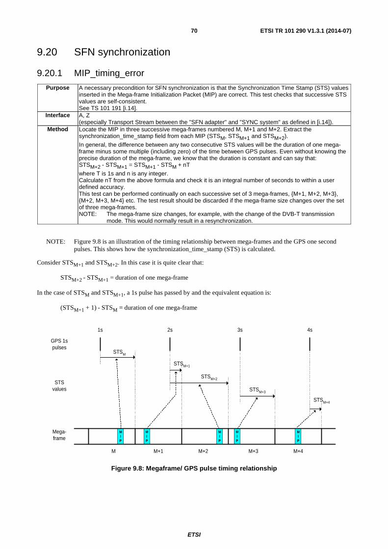
ETSI
ETSI TR 101 290 V1.3.1 (2014-07) 70
9.20 SFN synchronization
9.20.1 MIP_timing_error
Purpose A necessary precondition for SFN synchronization is that the Synchronization Time Stamp (STS) values inserted in the Mega-frame Initialization Packet (MIP) are correct. This test checks that successive STS values are self-consistent. See TS 101 191 [i.14].
Interface A, Z (especially Transport Stream between the "SFN adapter" and "SYNC system" as defined in [i.14]).
Method Locate the MIP in three successive mega-frames numbered M, M+1 and M+2. Extract the synchronization_time_stamp field from each MIP (STSM, STSM+1 and STSM+2).
In general, the difference between any two consecutive STS values will be the duration of one mega-frame minus some multiple (including zero) of the time between GPS pulses. Even without knowing the precise duration of the mega-frame, we know that the duration is constant and can say that: STSM+2 - STSM+1 = STSM+1 - STSM + nT
where T is 1s and n is any integer. Calculate nT from the above formula and check it is an integral number of seconds to within a user defined accuracy. This test can be performed continually on each successive set of 3 mega-frames, {M+1, M+2, M+3}, {M+2, M+3, M+4} etc. The test result should be discarded if the mega-frame size changes over the set of three mega-frames. NOTE: The mega-frame size changes, for example, with the change of the DVB-T transmission
mode. This would normally result in a resynchronization.
NOTE: Figure 9.8 is an illustration of the timing relationship between mega-frames and the GPS one second pulses. This shows how the synchronization_time_stamp (STS) is calculated.
Consider STSM+1 and STSM+2. In this case it is quite clear that:
STSM+2 - STSM+1 = duration of one mega-frame
In the case of STSM and STSM+1, a 1s pulse has passed by and the equivalent equation is:
(STSM+1 + 1) - STSM = duration of one mega-frame
GPS 1spulses
Mega-frame
MIP
MIP
MIP
MIP
MIP
STSvalues
1s 2s 3s 4s
STSM
STSM+1
STSM+2
STSM+3
STSM+4
M M+1 M+2 M+3 M+4
Figure 9.8: Megaframe/ GPS pulse timing relationship
ETSI
ETSI TR 101 290 V1.3.1 (2014-07) 71
9.20.2 MIP_structure_error
Purpose This test verifies that the syntax of the MIP complies with the specification in TS 101 191 [i.14].
Interface A, Z Method For each transport packet carried on PID 0x15 in the transport stream, the following
checks are performed: The transport_packet_header should comply with TS 101 191 [i.14] clause 6, table 1, and ISO/IEC 13818-1 [i.1] clause 2.4.3.2, tables 2 and 3. All length fields should be consistent to provide a proper length packet. This includes section_length (which also should not exceed 182), individual_addressing_length (which should match the length of the loops for each transmitter), function_loop_length (which should match the sum of the size of each of the functions), function_length (which should match the proper length of the function based upon the function tag). The synchronization_time_stamp and the maximum_delay should be in the range of 0x0 to 0x98967F. The CRC_32 field should match the CRC calculated for the MIP data.
9.20.3 MIP_presence_error
Purpose
This test verifies that the MIP is inserted into the transport stream only once per mega-frame.
Interface A, Z Method
The following checks are performed: Extra MIP – For every MIPN (where N > 1), signal an error if it arrives within the number
of packets indicated by the pointer field of MIPN-1.
Missing MIP - For each MIP received, calculate the mega-frame size from the parameters in the tps_mip. The latest two values of the mega-frame size are stored. After every MIPN is received (where N > 1), signal an error if a MIPN+1 is not received
before K + R packets are received after MIPN, where K is the pointer value of MIPN and
R is mega-frame size in packets from the previous MIPN-1.
9.20.4 MIP_pointer_error
Purpose
The MIP insertion can be at any location in the mega-frame. If the insertion is periodic as defined in the MIP, the MIP location in the mega-frame is constant over time. The MIP can be used to determine the mega-frame size and where each mega-frame starts and ends in the transport stream thanks to the pointer field verified by this test.
Interface A, Z Method
For each MIP received, calculate the mega-frame size from the parameters in the tps_mip. The latest three values of the mega-frame size are stored. For every MIPN that
is received (where N > 2), signal an error if the pointer value (PN) of MIPN does not hold
in the following equation: PN = PN-1 + MFN-2 - (iN - iN-1)
Where MFN-2 is the size of the Nth mega-frame in packets but is calculated from MIPN-
2, and iN is the packet index for MIPN.
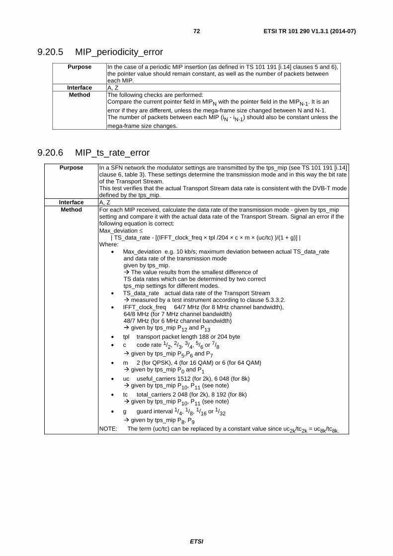
ETSI
ETSI TR 101 290 V1.3.1 (2014-07) 72
9.20.5 MIP_periodicity_error
Purpose
In the case of a periodic MIP insertion (as defined in TS 101 191 [i.14] clauses 5 and 6), the pointer value should remain constant, as well as the number of packets between each MIP.
Interface A, Z Method
The following checks are performed: Compare the current pointer field in MIPN with the pointer field in the MIPN-1. It is an
error if they are different, unless the mega-frame size changed between N and N-1. The number of packets between each MIP (iN - iN-1) should also be constant unless the
mega-frame size changes.
9.20.6 MIP_ts_rate_error
Purpose In a SFN network the modulator settings are transmitted by the tps_mip (see TS 101 191 [i.14] clause 6, table 3). These settings determine the transmission mode and in this way the bit rate of the Transport Stream. This test verifies that the actual Transport Stream data rate is consistent with the DVB-T mode defined by the tps_mip.
Interface A, Z Method For each MIP received, calculate the data rate of the transmission mode - given by tps_mip
setting and compare it with the actual data rate of the Transport Stream. Signal an error if the following equation is correct: Max_deviation ≤ | TS_data_rate - [(IFFT_clock_freq × tpl /204 × c × m × (uc/tc) )/(1 + g)] | Where:
• Max_deviation e.g. 10 kb/s; maximum deviation between actual TS_data_rate and data rate of the transmission mode given by tps_mip. � The value results from the smallest difference of TS data rates which can be determined by two correct tps_mip settings for different modes.
• TS_data_rate actual data rate of the Transport Stream � measured by a test instrument according to clause 5.3.3.2.
• IFFT_clock_freq 64/7 MHz (for 8 MHz channel bandwidth), 64/8 MHz (for 7 MHz channel bandwidth) 48/7 MHz (for 6 MHz channel bandwidth) � given by tps_mip P12 and P13
• tpl transport packet length 188 or 204 byte • c code rate 1/2, 2/3, 3/4, 5/6 or 7/8
� given by tps_mip P5,P6 and P7
• m 2 (for QPSK), 4 (for 16 QAM) or 6 (for 64 QAM) � given by tps_mip P0 and P1
• uc useful_carriers 1512 (for 2k), 6 048 (for 8k) � given by tps_mip P10, P11 (see note)
• tc total_carriers 2 048 (for 2k), 8 192 (for 8k) � given by tps_mip P10, P11 (see note)
• g guard interval 1/4, 1/8, 1/16 or 1/32
� given by tps_mip P8, P9
NOTE: The term (uc/tc) can be replaced by a constant value since uc2k/tc2k = uc8k/tc8k.
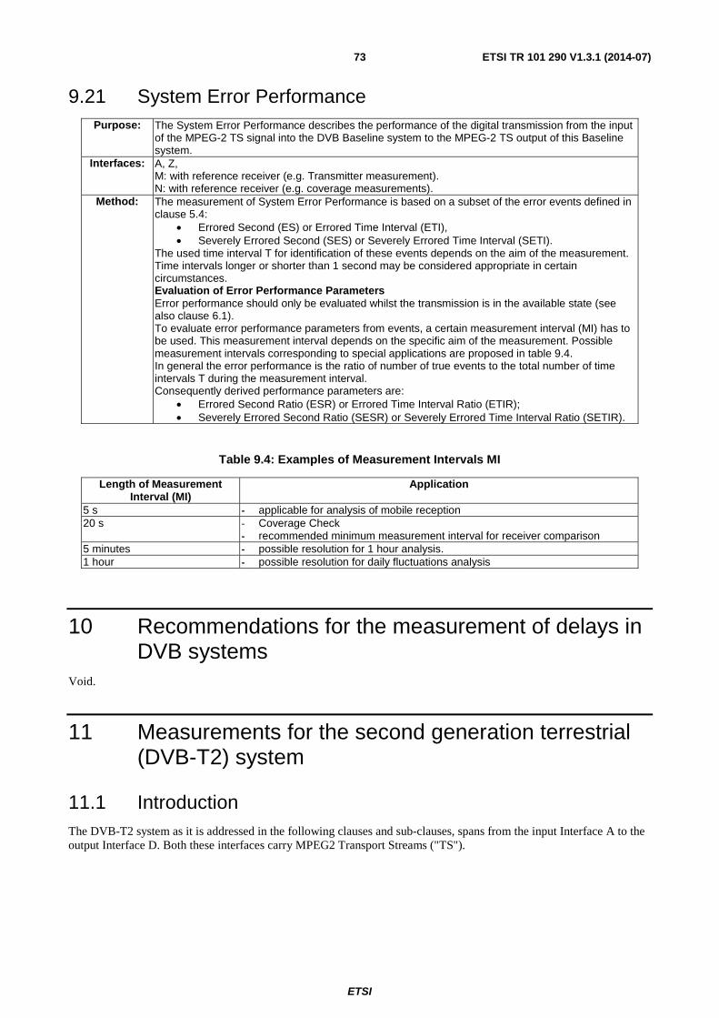
ETSI
ETSI TR 101 290 V1.3.1 (2014-07) 73
9.21 System Error Performance Purpose: The System Error Performance describes the performance of the digital transmission from the input
of the MPEG-2 TS signal into the DVB Baseline system to the MPEG-2 TS output of this Baseline system.
Interfaces: A, Z, M: with reference receiver (e.g. Transmitter measurement). N: with reference receiver (e.g. coverage measurements).
Method: The measurement of System Error Performance is based on a subset of the error events defined in clause 5.4:
• Errored Second (ES) or Errored Time Interval (ETI), • Severely Errored Second (SES) or Severely Errored Time Interval (SETI).
The used time interval T for identification of these events depends on the aim of the measurement. Time intervals longer or shorter than 1 second may be considered appropriate in certain circumstances. Evaluation of Error Performance Parameters Error performance should only be evaluated whilst the transmission is in the available state (see also clause 6.1). To evaluate error performance parameters from events, a certain measurement interval (MI) has to be used. This measurement interval depends on the specific aim of the measurement. Possible measurement intervals corresponding to special applications are proposed in table 9.4. In general the error performance is the ratio of number of true events to the total number of time intervals T during the measurement interval. Consequently derived performance parameters are:
• Errored Second Ratio (ESR) or Errored Time Interval Ratio (ETIR); • Severely Errored Second Ratio (SESR) or Severely Errored Time Interval Ratio (SETIR).
Table 9.4: Examples of Measurement Intervals MI
Length of Measurement Interval (MI)
Application
5 s - applicable for analysis of mobile reception 20 s - Coverage Check
- recommended minimum measurement interval for receiver comparison 5 minutes - possible resolution for 1 hour analysis. 1 hour - possible resolution for daily fluctuations analysis
10 Recommendations for the measurement of delays in DVB systems
Void.
11 Measurements for the second generation terrestrial (DVB-T2) system
11.1 Introduction The DVB-T2 system as it is addressed in the following clauses and sub-clauses, spans from the input Interface A to the output Interface D. Both these interfaces carry MPEG2 Transport Streams ("TS").
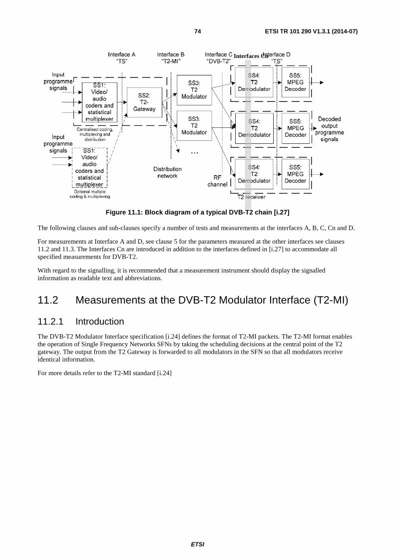
ETSI
ETSI TR 101 290 V1.3.1 (2014-07) 74
Figure 11.1: Block diagram of a typical DVB-T2 chain [i.27]
The following clauses and sub-clauses specify a number of tests and measurements at the interfaces A, B, C, Cn and D.
For measurements at Interface A and D, see clause 5 for the parameters measured at the other interfaces see clauses 11.2 and 11.3. The Interfaces Cn are introduced in addition to the interfaces defined in [i.27] to accommodate all specified measurements for DVB-T2.
With regard to the signalling, it is recommended that a measurement instrument should display the signalled information as readable text and abbreviations.
11.2 Measurements at the DVB-T2 Modulator Interface (T2-MI)
11.2.1 Introduction
The DVB-T2 Modulator Interface specification [i.24] defines the format of T2-MI packets. The T2-MI format enables the operation of Single Frequency Networks SFNs by taking the scheduling decisions at the central point of the T2 gateway. The output from the T2 Gateway is forwarded to all modulators in the SFN so that all modulators receive identical information.
For more details refer to the T2-MI standard [i.24]
Interfaces Cn
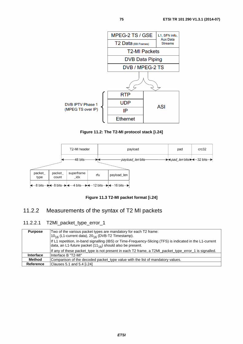
ETSI
ETSI TR 101 290 V1.3.1 (2014-07) 75
Figure 11.2: The T2-MI protocol stack [i.24]
Figure 11.3 T2-MI packet format [i.24]
11.2.2 Measurements of the syntax of T2 MI packets
11.2.2.1 T2MI_packet_type_error_1
Purpose Two of the various packet types are mandatory for each T2 frame: 1016 (L1-current data), 2016 (DVB-T2 Timestamp).
If L1 repetition, in-band signalling (IBS) or Time-Frequency-Slicing (TFS) is indicated in the L1-current data, an L1-future packet (1116) should also be present.
If any of these packet_type is not present in each T2 frame, a T2MI_packet_type_error_1 is signalled. Interface Interface B "T2-MI" Method Comparison of the decoded packet_type value with the list of mandatory values.
Reference Clauses 5.1 and 5.4 [i.24]
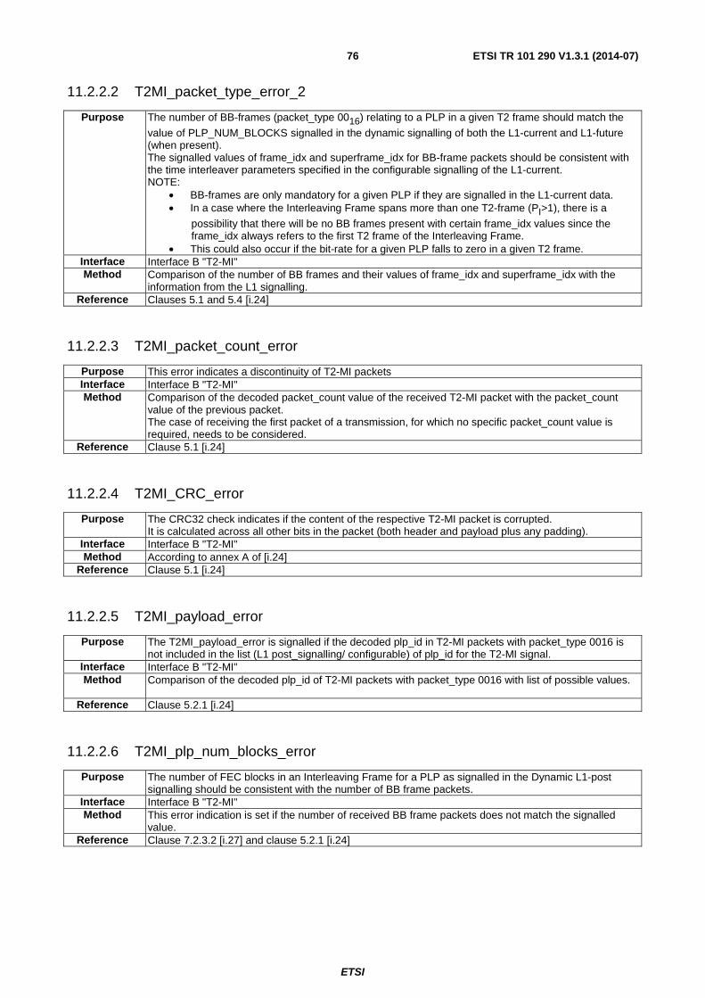
ETSI
ETSI TR 101 290 V1.3.1 (2014-07) 76
11.2.2.2 T2MI_packet_type_error_2
Purpose The number of BB-frames (packet_type 0016) relating to a PLP in a given T2 frame should match the
value of PLP_NUM_BLOCKS signalled in the dynamic signalling of both the L1-current and L1-future (when present). The signalled values of frame_idx and superframe_idx for BB-frame packets should be consistent with the time interleaver parameters specified in the configurable signalling of the L1-current. NOTE:
• BB-frames are only mandatory for a given PLP if they are signalled in the L1-current data. • In a case where the Interleaving Frame spans more than one T2-frame (PI>1), there is a
possibility that there will be no BB frames present with certain frame_idx values since the frame_idx always refers to the first T2 frame of the Interleaving Frame.
• This could also occur if the bit-rate for a given PLP falls to zero in a given T2 frame. Interface Interface B "T2-MI" Method Comparison of the number of BB frames and their values of frame_idx and superframe_idx with the
information from the L1 signalling. Reference Clauses 5.1 and 5.4 [i.24]
11.2.2.3 T2MI_packet_count_error
Purpose This error indicates a discontinuity of T2-MI packets Interface Interface B "T2-MI" Method Comparison of the decoded packet_count value of the received T2-MI packet with the packet_count
value of the previous packet. The case of receiving the first packet of a transmission, for which no specific packet_count value is required, needs to be considered.
Reference Clause 5.1 [i.24]
11.2.2.4 T2MI_CRC_error
Purpose The CRC32 check indicates if the content of the respective T2-MI packet is corrupted. It is calculated across all other bits in the packet (both header and payload plus any padding).
Interface Interface B "T2-MI" Method According to annex A of [i.24]
Reference Clause 5.1 [i.24]
11.2.2.5 T2MI_payload_error
Purpose The T2MI_payload_error is signalled if the decoded plp_id in T2-MI packets with packet_type 0016 is not included in the list (L1 post_signalling/ configurable) of plp_id for the T2-MI signal.
Interface Interface B "T2-MI" Method Comparison of the decoded plp_id of T2-MI packets with packet_type 0016 with list of possible values.
Reference Clause 5.2.1 [i.24]
11.2.2.6 T2MI_plp_num_blocks_error
Purpose The number of FEC blocks in an Interleaving Frame for a PLP as signalled in the Dynamic L1-post signalling should be consistent with the number of BB frame packets.
Interface Interface B "T2-MI" Method This error indication is set if the number of received BB frame packets does not match the signalled
value. Reference Clause 7.2.3.2 [i.27] and clause 5.2.1 [i.24]
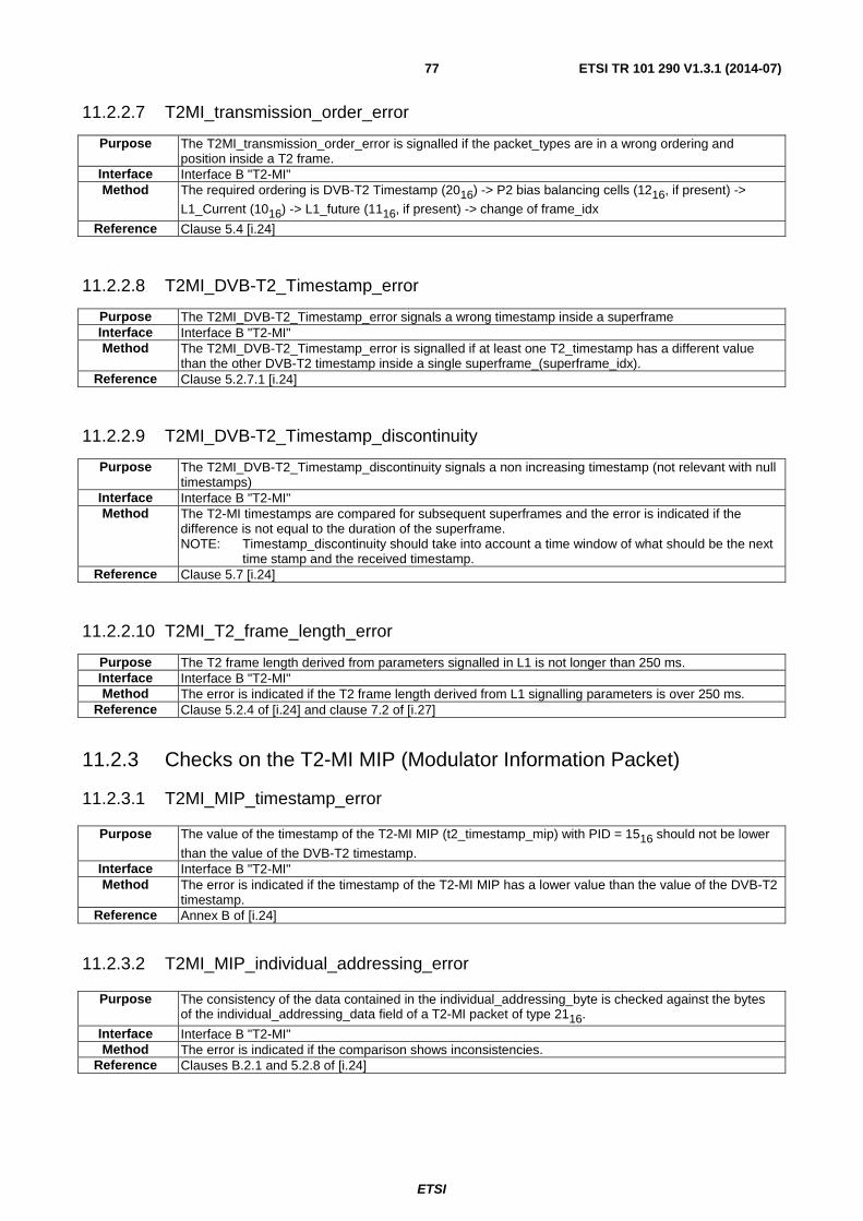
ETSI
ETSI TR 101 290 V1.3.1 (2014-07) 77
11.2.2.7 T2MI_transmission_order_error
Purpose The T2MI_transmission_order_error is signalled if the packet_types are in a wrong ordering and position inside a T2 frame.
Interface Interface B "T2-MI" Method The required ordering is DVB-T2 Timestamp (2016) -> P2 bias balancing cells (1216, if present) ->
L1_Current (1016) -> L1_future (1116, if present) -> change of frame_idx
Reference Clause 5.4 [i.24]
11.2.2.8 T2MI_DVB-T2_Timestamp_error
Purpose The T2MI_DVB-T2_Timestamp_error signals a wrong timestamp inside a superframe Interface Interface B "T2-MI" Method The T2MI_DVB-T2_Timestamp_error is signalled if at least one T2_timestamp has a different value
than the other DVB-T2 timestamp inside a single superframe_(superframe_idx). Reference Clause 5.2.7.1 [i.24]
11.2.2.9 T2MI_DVB-T2_Timestamp_discontinuity
Purpose The T2MI_DVB-T2_Timestamp_discontinuity signals a non increasing timestamp (not relevant with null timestamps)
Interface Interface B "T2-MI" Method The T2-MI timestamps are compared for subsequent superframes and the error is indicated if the
difference is not equal to the duration of the superframe. NOTE: Timestamp_discontinuity should take into account a time window of what should be the next
time stamp and the received timestamp. Reference Clause 5.7 [i.24]
11.2.2.10 T2MI_T2_frame_length_error
Purpose The T2 frame length derived from parameters signalled in L1 is not longer than 250 ms. Interface Interface B "T2-MI" Method The error is indicated if the T2 frame length derived from L1 signalling parameters is over 250 ms.
Reference Clause 5.2.4 of [i.24] and clause 7.2 of [i.27]
11.2.3 Checks on the T2-MI MIP (Modulator Information Packet)
11.2.3.1 T2MI_MIP_timestamp_error
Purpose The value of the timestamp of the T2-MI MIP (t2_timestamp_mip) with PID = 1516 should not be lower
than the value of the DVB-T2 timestamp. Interface Interface B "T2-MI" Method The error is indicated if the timestamp of the T2-MI MIP has a lower value than the value of the DVB-T2
timestamp. Reference Annex B of [i.24]
11.2.3.2 T2MI_MIP_individual_addressing_error
Purpose The consistency of the data contained in the individual_addressing_byte is checked against the bytes of the individual_addressing_data field of a T2-MI packet of type 2116.
Interface Interface B "T2-MI" Method The error is indicated if the comparison shows inconsistencies.
Reference Clauses B.2.1 and 5.2.8 of [i.24]
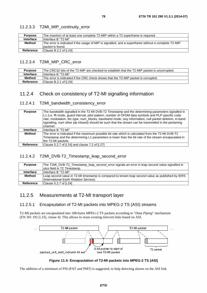
ETSI
ETSI TR 101 290 V1.3.1 (2014-07) 78
11.2.3.3 T2MI_MIP_continuity_error
Purpose The insertion of at least one complete T2-MIP within a T2 superframe is required. Interface Interface B "T2-MI" Method The error is indicated if the usage of MIP is signalled, and a superframe without a complete T2-MIP
packet is found. Reference Clause B.2.2 of [i.24]
11.2.3.4 T2MI_MIP_CRC_error
Purpose The CRC32 bits of the T2-MIP are checked to establish that the T2-MIP packet is uncorrupted. Interface Interface B "T2-MI" Method The error is indicated if the CRC check shows that the T2-MIP packet is corrupted.
Reference Clause B.2.1 of [i.24]
11.2.4 Check on consistency of T2-MI signalling information
11.2.4.1 T2MI_bandwidth_consistency_error
Purpose The bandwidth signalled in the T2-MI DVB-T2 Timestamp and the determining parameters signalled in L1 (i.e. fft mode, guard interval, pilot pattern, number of OFDM data symbols and PLP specific code rate, modulation, fec type, num_blocks, baseband mode, issy information, null packet deletion, in-band signalling, num other plp inband) should be such that the stream can be transmitted in the pertaining channel.
Interface Interface B "T2-MI" Method The error is indicated if the maximum possible bit rate which is calculated from the T2-MI DVB-T2
Timestamp and the determining L1 parameters is lower than the bit rate of the stream encapsulated in the T2-MI packets.
Reference Clause 5.2.7 of [i.24] and clause 7.2 of [i.27]
11.2.4.2 T2MI_DVB-T2_Timestamp_leap_second_error
Purpose The T2MI_DVB-T2_Timestamp_leap_second_error signals an error in leap second value signalled in utco field in T2 Timestamp.
Interface Interface B "T2-MI" Method Leap second value in T2-MI timestamp is compared to known leap second value as published by IERS
(International Earth Rotation Service). Reference Clause 5.2.7 of [i.24]
11.2.5 Measurements at T2-MI transport layer
11.2.5.1 Encapsulation of T2-MI packets into MPEG-2 TS (ASI) streams
T2-MI packets are encapsulated into 188-bytes MPEG-2 TS packets according to "Data Piping" mechanism (EN 301 192 [i.33], clause 4). This allows to reuse existing telecom links based on ASI.
Figure 11.4: Encapsulation of T2-MI packets into MPEG-2 TS (ASI)
The addition of a minimum of PSI (PAT and PMT) is suggested, to help detecting alarms on the ASI link.
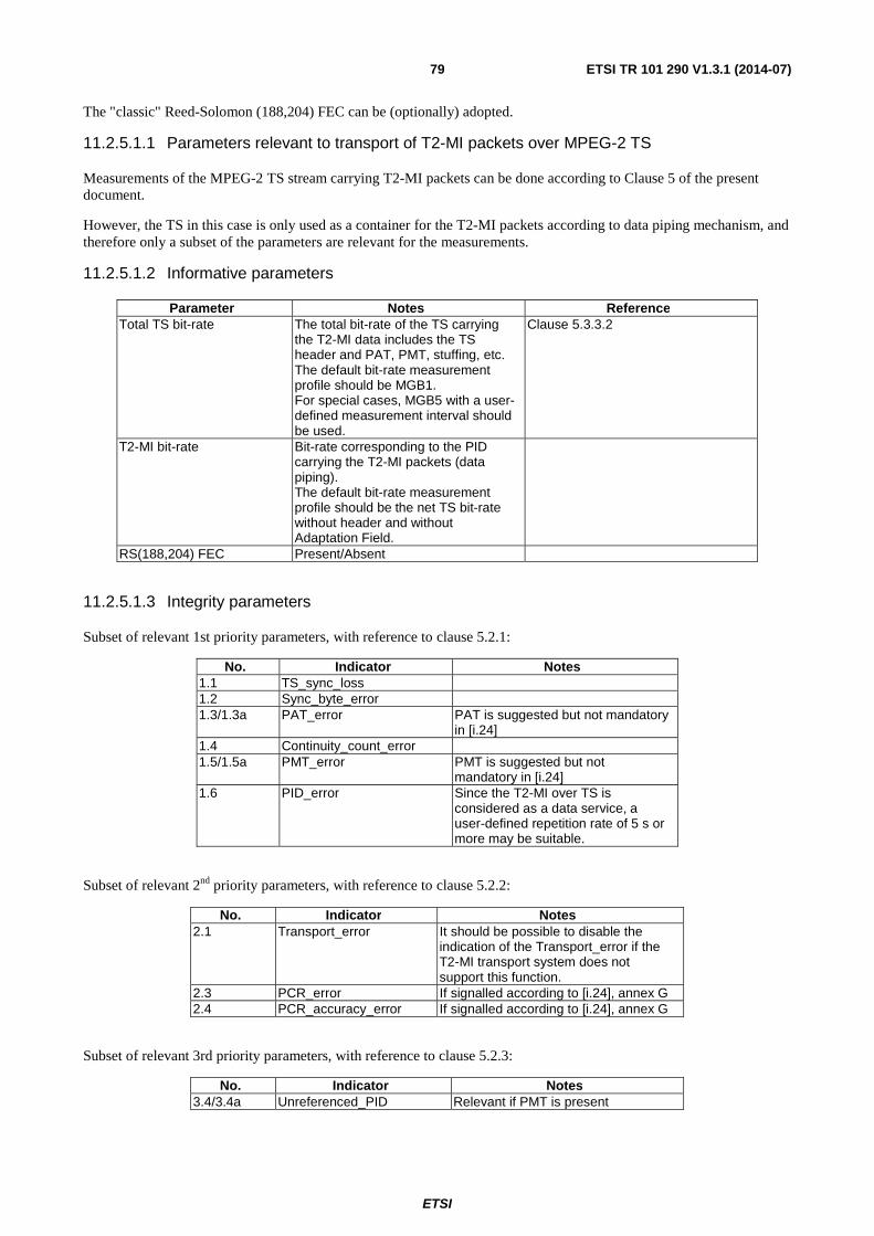
ETSI
ETSI TR 101 290 V1.3.1 (2014-07) 79
The "classic" Reed-Solomon (188,204) FEC can be (optionally) adopted.
11.2.5.1.1 Parameters relevant to transport of T2-MI packets over MPEG-2 TS
Measurements of the MPEG-2 TS stream carrying T2-MI packets can be done according to Clause 5 of the present document.
However, the TS in this case is only used as a container for the T2-MI packets according to data piping mechanism, and therefore only a subset of the parameters are relevant for the measurements.
11.2.5.1.2 Informative parameters
Parameter Notes Reference Total TS bit-rate The total bit-rate of the TS carrying
the T2-MI data includes the TS header and PAT, PMT, stuffing, etc. The default bit-rate measurement profile should be MGB1. For special cases, MGB5 with a user-defined measurement interval should be used.
Clause 5.3.3.2
T2-MI bit-rate Bit-rate corresponding to the PID carrying the T2-MI packets (data piping). The default bit-rate measurement profile should be the net TS bit-rate without header and without Adaptation Field.
RS(188,204) FEC Present/Absent
11.2.5.1.3 Integrity parameters
Subset of relevant 1st priority parameters, with reference to clause 5.2.1:
No. Indicator Notes 1.1 TS_sync_loss 1.2 Sync_byte_error 1.3/1.3a PAT_error PAT is suggested but not mandatory
in [i.24] 1.4 Continuity_count_error 1.5/1.5a PMT_error PMT is suggested but not
mandatory in [i.24] 1.6 PID_error Since the T2-MI over TS is
considered as a data service, a user-defined repetition rate of 5 s or more may be suitable.
Subset of relevant 2nd priority parameters, with reference to clause 5.2.2:
No. Indicator Notes 2.1 Transport_error It should be possible to disable the
indication of the Transport_error if the T2-MI transport system does not support this function.
2.3 PCR_error If signalled according to [i.24], annex G 2.4 PCR_accuracy_error If signalled according to [i.24], annex G
Subset of relevant 3rd priority parameters, with reference to clause 5.2.3:
No. Indicator Notes 3.4/3.4a Unreferenced_PID Relevant if PMT is present
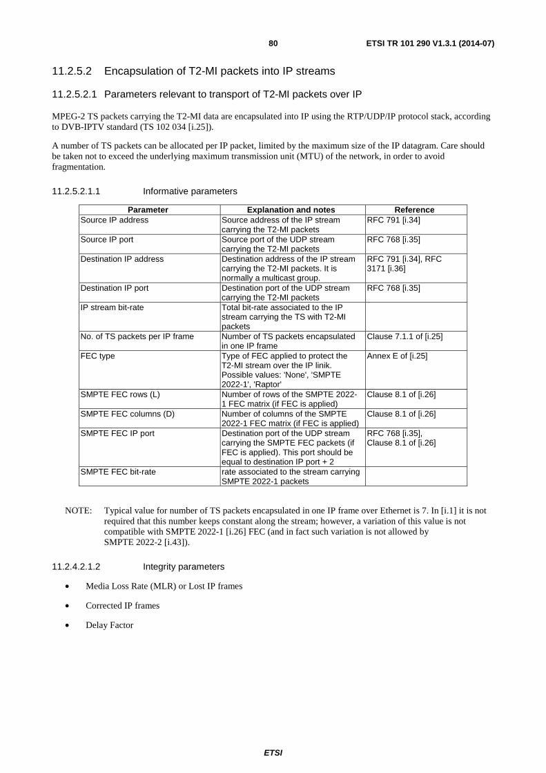
ETSI
ETSI TR 101 290 V1.3.1 (2014-07) 80
11.2.5.2 Encapsulation of T2-MI packets into IP streams
11.2.5.2.1 Parameters relevant to transport of T2-MI packets over IP
MPEG-2 TS packets carrying the T2-MI data are encapsulated into IP using the RTP/UDP/IP protocol stack, according to DVB-IPTV standard (TS 102 034 [i.25]).
A number of TS packets can be allocated per IP packet, limited by the maximum size of the IP datagram. Care should be taken not to exceed the underlying maximum transmission unit (MTU) of the network, in order to avoid fragmentation.
11.2.5.2.1.1 Informative parameters
Parameter Explanation and notes Reference Source IP address Source address of the IP stream
carrying the T2-MI packets RFC 791 [i.34]
Source IP port Source port of the UDP stream carrying the T2-MI packets
RFC 768 [i.35]
Destination IP address Destination address of the IP stream carrying the T2-MI packets. It is normally a multicast group.
RFC 791 [i.34], RFC 3171 [i.36]
Destination IP port Destination port of the UDP stream carrying the T2-MI packets
RFC 768 [i.35]
IP stream bit-rate Total bit-rate associated to the IP stream carrying the TS with T2-MI packets
No. of TS packets per IP frame Number of TS packets encapsulated in one IP frame
Clause 7.1.1 of [i.25]
FEC type Type of FEC applied to protect the T2-MI stream over the IP linik. Possible values: 'None', 'SMPTE 2022-1', 'Raptor'
Annex E of [i.25]
SMPTE FEC rows (L) Number of rows of the SMPTE 2022-1 FEC matrix (if FEC is applied)
Clause 8.1 of [i.26]
SMPTE FEC columns (D) Number of columns of the SMPTE 2022-1 FEC matrix (if FEC is applied)
Clause 8.1 of [i.26]
SMPTE FEC IP port Destination port of the UDP stream carrying the SMPTE FEC packets (if FEC is applied). This port should be equal to destination IP port + 2
RFC 768 [i.35], Clause 8.1 of [i.26]
SMPTE FEC bit-rate rate associated to the stream carrying SMPTE 2022-1 packets
NOTE: Typical value for number of TS packets encapsulated in one IP frame over Ethernet is 7. In [i.1] it is not required that this number keeps constant along the stream; however, a variation of this value is not compatible with SMPTE 2022-1 [i.26] FEC (and in fact such variation is not allowed by SMPTE 2022-2 [i.43]).
11.2.4.2.1.2 Integrity parameters
• Media Loss Rate (MLR) or Lost IP frames
• Corrected IP frames
• Delay Factor

ETSI
ETSI TR 101 290 V1.3.1 (2014-07) 81
11.2.5.2.1.2.1 Media Delivery Index - Media Loss Rate (MDI-MLR)
Purpose Number of IP packets lost per second, after error recovery mechanisms, if any. This parameter is part of the MDI (Media Delivery Index) parameter. Error if > 0.
Interface Interface B "T2-MI" – IP transport layer Method The Continuity Counter field of the inner MPEG-2 TS stream can be used. Under error free
conditions, the sequence numbers increment. Counting any missing sequence numbers every second will produce the packets lost per second. Alternatively, the RTP layer information can be used as a supplement for the UDP protocol. RTP also uses sequence numbers and this number also increments with every packet. The same method as above, of counting missing sequence numbers may be used.
Reference Clause 3.2 of RFC 4445 [i.37]
11.2.5.2.1.2.2 Lost IP frames
Purpose Alternative option to represent packet loss with respect to MLR. Cumulative number of IP packets lost per second, after error recovery mechanisms, if any. Error if > 0.
Interface Interface B "T2-MI" – IP transport layer Method The Continuity Counter field of the inner MPEG-2 TS stream can be used. Under error free
conditions, the sequence numbers increment. Counting any missing sequence numbers every second will produce the packets lost per second. Alternatively, the RTP layer information can be used as a supplement for the UDP protocol. RTP also uses sequence numbers and this number also increments with every packet. The same method as above, of counting missing sequence numbers may be used.
Reference Clause 3.2 of RFC 4445 [i.37]
11.2.5.2.1.2.3 Corrected IP frames
Purpose The value of Lost IP frames + Corrected IP frames gives an indication of the capabilities of the FEC mechanism.
Interface Interface B "T2-MI" – IP transport layer Method In case of FEC, number of IP packets corrected by the FEC mechanism.
Reference
11.2.5.2.1.2.4 Media Delivery Index - Delay Factor (MDI-DF)
Purpose Maximum difference, observed at the end of each media stream packet, between the arrival of media data and the drain of media data, over a calculation interval (typically 1 s). This assumes the drain rate is the nominal constant traffic rate for constant bit rate. The DF gives a good approximation of the needed buffer at receiving side to compensate for network jitter cumulated over the calculation interval. This parameter is part of the Media Delivery Index (MDI) parameter.
Interface Interface B "T2-MI" – IP transport layer Method Consider a virtual buffer VB used to buffer received packets of a stream. When a packet P(i) arrives
during a calculation interval, compute two VB values, VB(i,pre) and VB(i,post), defined as: • VB(i,pre) = sum (Sj) - MR * Ti; where j=1..i-1 • VB(i,post) = VB(i,pre) + Si
where Sj is the media payload size of the jth packet, Ti is the relative time at which packet i arrives in the interval, and MR is the nominal media rate. VB(i,pre) is the Virtual Buffer size just before the arrival of P(i). VB(i,post) is the Virtual Buffer size just after the arrival of P(i). The initial condition of VB(0) = 0 is used at the beginning of each measurement interval. A measurement interval is defined from just after the time of arrival of the last packet during a nominal period (typically 1 second) to the time just after the arrival of the last packet of the next nominal period. During a measurement interval, if k packets are received, then there are 2*k+1 VB values used in deriving VB(max) and VB(min). After determining VB(max) and VB(min) from the 2k+1 VB samples, DF for the measurement interval is computed and displayed as:
• DF = [VB(max) - VB(min)]/ MR Reference Clause 3.1 of RFC 4445 [i.37]
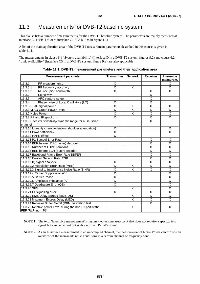
ETSI
ETSI TR 101 290 V1.3.1 (2014-07) 82
11.3 Measurements for DVB-T2 baseline system
This clause lists a number of measurements for the DVB-T2 baseline system. The parameters are mainly measured at interface C "DVB-T2" or at interface C1 "T2-IQ" as in figure 11.1.
A list of the main application area of the DVB-T2 measurement parameters described in this clause is given in table 11.1.
The measurements in clause 6.1 "System availability" (Interface D in a DVB-T2 system, figures 9.2) and clause 6.2 "Link availability" (Interface C5 in a DVB-T2 system, figure 9.2) are also applicable.
Table 11.1: DVB-T2 measurement parameters and their application area
Measurement parameter Transmitter Network Receiver In-service measurem.
11.3.1 RF measurements X X 11.3.1.1 RF frequency accuracy X X X 11.3.1.2 RF occupied bandwidth X X X 11.3.2 Selectivity X 11.3.3 AFC capture range X 11.3.4 Phase noise of Local Oscillators (LO) X X 11.3.5 RF/IF signal power X X X X 11.3.6 MISO Group Power Ratio X X X X 11.3.7 Noise Power X X X X 11.3.8 RF and IF spectrum X X X 11.3.9 Receiver sensitivity/ dynamic range for a Gaussian channel
X
11.3.10 Linearity characterization (shoulder attenuation) X X 11.3.11 Power efficiency X X 11.3.12 PAPR effect X 11.3.13 P1 Symbol Error Rate X X 11.3.14 BER before LDPC (inner) decoder X X 11.3.15 Number of LDPC iterations X X 11.3.16 BER before BCH (outer) decoder X X 11.3.17 Baseband Frame Error Rate BBFER X X 11.3.18 Errored Second Ratio ESR X X 11.3.19 IQ signal analysis X X X 11.3.19.2 Modulation Error Ratio (MER) X X X X 11.3.19.3 Signal to Interference Noise Ratio (SINR) X X X X 11.3.19.4 Carrier Suppression (CS) X X 11.3.19.5 Carrier Phase X X 11.3.19.6 Amplitude Imbalance (AI) X X 11.3.19.7 Quadrature Error (QE) X X 11.3.20 SFN X X 11.3.21 L1 signalling error X X X 11.3.22 RMS Delay-Spread (RMS-DS) X X X 11.3.23 Maximum Excess Delay (MED) X X X 11.3.24 Receiver Buffer Model (RBM) validation test X 11.3.25 Relative power Level during the non-P1 part of the FEF (RLF_non_P1)
X X
NOTE 1: The term 'In-service measurement' is understood as a measurement that does not require a specific test signal but can be carried out with a normal DVB-T2 signal.
NOTE 2: As an In-service measurement in an unoccupied channel, the measurement of Noise Power can provide an overview of the man-made noise conditions in a certain channel or frequency band.

ETSI
ETSI TR 101 290 V1.3.1 (2014-07) 83
Figure 11.5: Simplified block diagram of a DVB-T2 transmitter
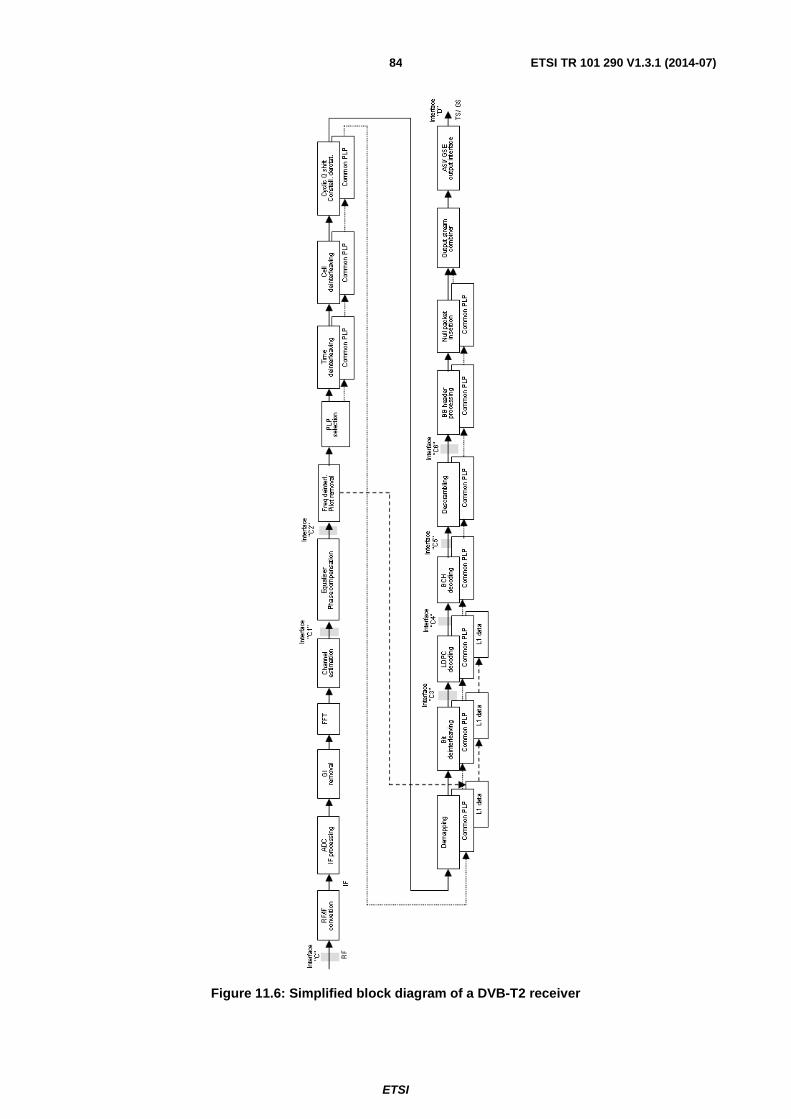
ETSI
ETSI TR 101 290 V1.3.1 (2014-07) 84
Figure 11.6: Simplified block diagram of a DVB-T2 receiver

ETSI
ETSI TR 101 290 V1.3.1 (2014-07) 85
11.3.1 RF measurements
The measurement of some basic parameters of the DVB-T2 OFDM signal may be carried out at the RF layer with a test receiver, a spectrum analyser or similar instruments.
11.3.1.1 RF frequency accuracy
Purpose Successful processing of OFDM signals requires that certain carrier frequency accuracy be maintained at the transmitter. Specific network operations modes such as SFN require high accuracy of the carrier frequency.
Interface C Method The measurement of the RF frequency accuracy determines the centre frequency of the signal, i.e. the
positioning of the signal in the RF channel. a) Spectrum analyser method: the centre frequency is derived from the frequencies measured
for the continual pilots and/ or the edge pilots. b) Test receiver method: the centre frequency is derived from the digital samples after the test
receiver has synchronized to the incoming DVB-T2 signal. In this case, the accuracy is typically expressed as 'Carrier Offset' and given in Hz or ppm.
Reference Clauses 9.2.4, 9.2.5 of [i.27]
NOTE: In any case, the usage of a high-precision reference frequency, e.g. 10 MHz, may be helpful.
11.3.1.2 RF occupied bandwidth
Purpose The measurement of the occupied bandwidth allows the verification of the correct sampling frequency at the modulator.
Interface C Method The occupied bandwidth is calculated from the measurements of the frequencies of the edge pilots
and/ or continual pilots of the DVB-T2 signal. a) Spectrum analyser method: if the frequency of the edge carriers is known then the related
values for the occupied bandwidth may be calculated. Denoting the edge pilot frequencies as Fmin and Fmax the occupied bandwidth is appropriately OB = Fmax - Fmin+ 1/TU.
b) Test receiver method: the occupied bandwidth is derived from the digital samples after the test receiver has synchronized to the incoming DVB-T2 signal.
Reference Clause 9.2.5 of [i.27]
11.3.2 Selectivity
Purpose To identify the capability of the receiver to reject out-of-channel interference. Interface The measurement of the signal input level and the interferer should be carried out at the interface C,
using interface C3 or C4 for the BER monitoring. Method The input power is adjusted to 10 dB above the minimum input power as defined in "Receiver
sensitivity" (see clause 11.3.9). The C/I threshold needed for QEF operation should be measured as a function of the frequency of a CW interferer. The failure point is defined as ESR5. ESR (Errored Second Ratio) is defined in clause 11.3.18. One errored second during a time interval of 20 seconds is given as ESR5 (5 % of the seconds are errored). Alternatively, the QEF point is used that is defined as BER after LDPC = 10-7. Since this measurement is time-consuming, the BER after LDPC = 10-4 is measured and the associated C/N value is increased by 0,2 dB. This corresponds to a BER after BCH = 10-11.
Reference Clause 6.1.2 of [i.27]

ETSI
ETSI TR 101 290 V1.3.1 (2014-07) 86
11.3.3 AFC capture range
Purpose To determine the frequency range over which the receiver will acquire overall lock. Interface C for the application of the test signal; C1 or C2 for the test of receiver synchronization Method A signal is applied to the input of the receiver, at a level 10 dB above the minimum input power as
defined in "Receiver sensitivity" (see clause 11.3.9). The signal is frequency shifted in steps (from below and above) towards a nominal value, whilst forcing the receiver to re-acquire after each step. Correct reception is assumed if after each step:
a) the receiver can synchronize to the applied DVB-T2 signal, or if this is not indicated, b) the failure point is defined as ESR5.
ESR (Errored Second Ratio) is defined in clause 11.3.18. One errored second during a time interval of 20 seconds is given as ESR5 (5 % of the seconds are errored). Alternatively, the QEF point is used that is defined as BER after LDPC = 10-7. Since this measurement is time-consuming, the BER after LDPC = 10-4 is measured and the associated C/N value is increased by 0,2 dB. This corresponds to a BER after BCH = 10-11.
Reference Clause 5.1.7 of [i.27]
11.3.4 Phase noise of Local Oscillators (LO)
Purpose Phase noise can be introduced at the transmitter, at any frequency converter or by the receiver. In an OFDM system the phase noise can cause Common Phase Error (CPE) which affects all carriers simultaneously, and which can be minimized or corrected by using the continual pilots. However the noise-like Inter-Carrier Interference (ICI) cannot be corrected. This measurement may be useful for manufacturing, incoming inspection and maintenance of modulators, transmitters, up/ down converters and receivers, either professional or consumer type.
Interface Any access to Local Oscillators (LO), in transmitters, converters and receivers. Method Phase noise can be measured with a spectrum analyser, a vector analyser or a phase noise test set.
Reference n/a
11.3.5 RF/IF signal power
Purpose Signal power, or wanted power, measurement is required to set and check signal levels at the transmitter and receiver sites.
Interface C Method The signal power of a DVB-T2 signal is defined as the mean power of the signal as would be measured
with a thermal power sensor. In the case of received signals care should be taken to limit the measurement to the bandwidth at the wanted signal. When using a spectrum analyser or a calibrated receiver, it should integrate the signal power within the nominal bandwidth of the signal (n × fSPACING)
where n is the number of carriers. Note that some spectrum analyser may not automatically compensate for the applied Resolution Bandwidth so that a manual correction may be applicable.
Reference n/a
11.3.6 MISO Group Power Ratio
Purpose The MISO Group Power Ratio (MGPR) is required to check the presence of both MISO Groups within a network.
Interface C Method The MGPR is defined as the RF signal power for MISO Group 1 divided by the RF signal power for
MISO Group 2. NOTE: The value should be given in dB. The MGPR may be negative if the signals of MISO Group
2 are received with higher input level than the signals of MISO Group 1. The MGPR takes the value of ±∞ in the presence of one MISO Group.
For the display of the power levels of the paths of both MISO groups, the use of different colours for the figures or the diagram components (e.g. power level over delay) is recommended.
Reference Clause 9.1 of [i.27]
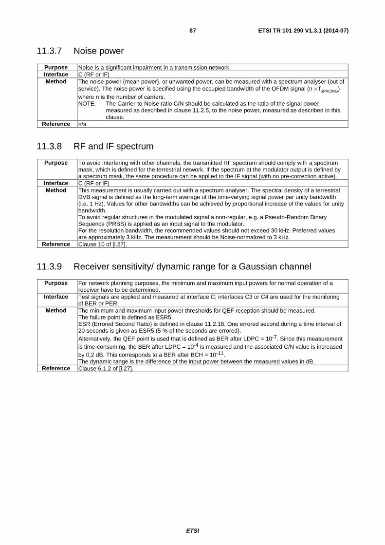
ETSI
ETSI TR 101 290 V1.3.1 (2014-07) 87
11.3.7 Noise power
Purpose Noise is a significant impairment in a transmission network. Interface C (RF or IF) Method The noise power (mean power), or unwanted power, can be measured with a spectrum analyser (out of
service). The noise power is specified using the occupied bandwidth of the OFDM signal (n × fSPACING) where n is the number of carriers. NOTE: The Carrier-to-Noise ratio C/N should be calculated as the ratio of the signal power,
measured as described in clause 11.2.5, to the noise power, measured as described in this clause.
Reference n/a
11.3.8 RF and IF spectrum
Purpose To avoid interfering with other channels, the transmitted RF spectrum should comply with a spectrum mask, which is defined for the terrestrial network. If the spectrum at the modulator output is defined by a spectrum mask, the same procedure can be applied to the IF signal (with no pre-correction active).
Interface C (RF or IF) Method This measurement is usually carried out with a spectrum analyser. The spectral density of a terrestrial
DVB signal is defined as the long-term average of the time-varying signal power per unity bandwidth (i.e. 1 Hz). Values for other bandwidths can be achieved by proportional increase of the values for unity bandwidth. To avoid regular structures in the modulated signal a non-regular, e.g. a Pseudo-Random Binary Sequence (PRBS) is applied as an input signal to the modulator. For the resolution bandwidth, the recommended values should not exceed 30 kHz. Preferred values are approximately 3 kHz. The measurement should be Noise-normalized to 3 kHz.
Reference Clause 10 of [i.27].
11.3.9 Receiver sensitivity/ dynamic range for a Gaussian channel
Purpose For network planning purposes, the minimum and maximum input powers for normal operation of a receiver have to be determined.
Interface Test signals are applied and measured at interface C; interfaces C3 or C4 are used for the monitoring of BER or PER.
Method The minimum and maximum input power thresholds for QEF reception should be measured. The failure point is defined as ESR5. ESR (Errored Second Ratio) is defined in clause 11.2.18. One errored second during a time interval of 20 seconds is given as ESR5 (5 % of the seconds are errored). Alternatively, the QEF point is used that is defined as BER after LDPC = 10-7. Since this measurement is time-consuming, the BER after LDPC = 10-4 is measured and the associated C/N value is increased by 0,2 dB. This corresponds to a BER after BCH = 10-11. The dynamic range is the difference of the input power between the measured values in dB.
Reference Clause 6.1.2 of [i.27].
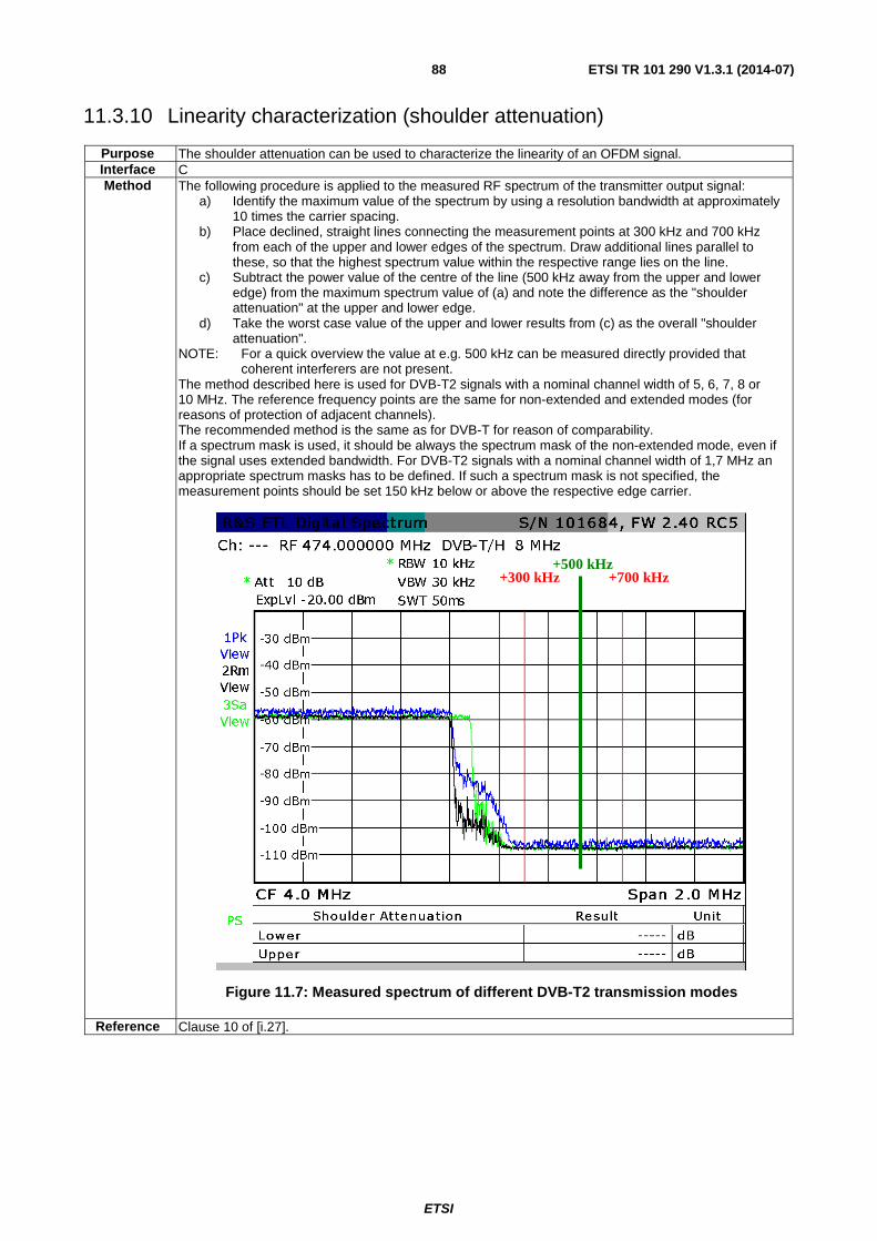
ETSI
ETSI TR 101 290 V1.3.1 (2014-07) 88
11.3.10 Linearity characterization (shoulder attenuation)
Purpose The shoulder attenuation can be used to characterize the linearity of an OFDM signal. Interface C Method The following procedure is applied to the measured RF spectrum of the transmitter output signal:
a) Identify the maximum value of the spectrum by using a resolution bandwidth at approximately 10 times the carrier spacing.
b) Place declined, straight lines connecting the measurement points at 300 kHz and 700 kHz from each of the upper and lower edges of the spectrum. Draw additional lines parallel to these, so that the highest spectrum value within the respective range lies on the line.
c) Subtract the power value of the centre of the line (500 kHz away from the upper and lower edge) from the maximum spectrum value of (a) and note the difference as the "shoulder attenuation" at the upper and lower edge.
d) Take the worst case value of the upper and lower results from (c) as the overall "shoulder attenuation".
NOTE: For a quick overview the value at e.g. 500 kHz can be measured directly provided that coherent interferers are not present.
The method described here is used for DVB-T2 signals with a nominal channel width of 5, 6, 7, 8 or 10 MHz. The reference frequency points are the same for non-extended and extended modes (for reasons of protection of adjacent channels). The recommended method is the same as for DVB-T for reason of comparability. If a spectrum mask is used, it should be always the spectrum mask of the non-extended mode, even if the signal uses extended bandwidth. For DVB-T2 signals with a nominal channel width of 1,7 MHz an appropriate spectrum masks has to be defined. If such a spectrum mask is not specified, the measurement points should be set 150 kHz below or above the respective edge carrier.
Figure 11.7: Measured spectrum of different DVB-T2 transmission modes
Reference Clause 10 of [i.27].
+300 kHz +700 kHz +500 kHz

ETSI
ETSI TR 101 290 V1.3.1 (2014-07) 89
11.3.11 Power efficiency
Purpose To compare the overall efficiency of DVB transmitters. Interface C Method Power efficiency is defined as the ratio of the DVB output power to the total power consumption of the
chain from TS input to the RF signal output including all necessary equipment for operation such as blowers, transformers etc. (and is usually quoted in % terms). The operational channel and the environmental conditions need to be specified.
Reference n/a
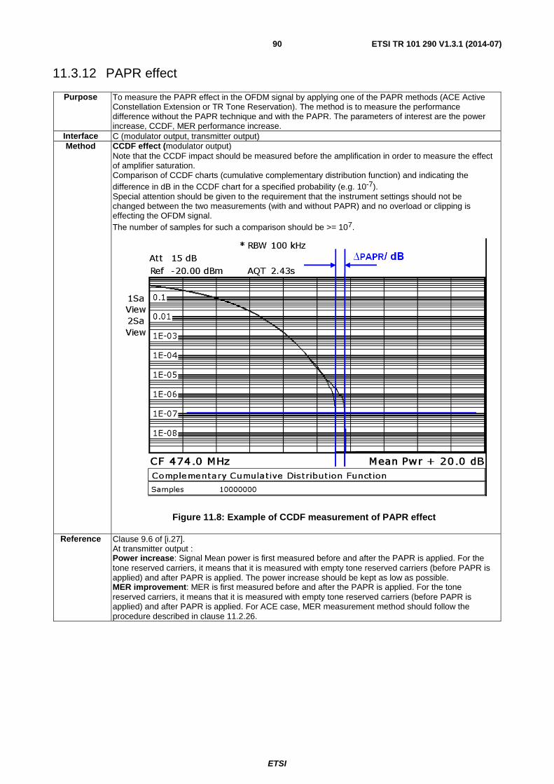
ETSI
ETSI TR 101 290 V1.3.1 (2014-07) 90
11.3.12 PAPR effect
Purpose To measure the PAPR effect in the OFDM signal by applying one of the PAPR methods (ACE Active Constellation Extension or TR Tone Reservation). The method is to measure the performance difference without the PAPR technique and with the PAPR. The parameters of interest are the power increase, CCDF, MER performance increase.
Interface C (modulator output, transmitter output) Method CCDF effect (modulator output)
Note that the CCDF impact should be measured before the amplification in order to measure the effect of amplifier saturation. Comparison of CCDF charts (cumulative complementary distribution function) and indicating the difference in dB in the CCDF chart for a specified probability (e.g. 10-7). Special attention should be given to the requirement that the instrument settings should not be changed between the two measurements (with and without PAPR) and no overload or clipping is effecting the OFDM signal. The number of samples for such a comparison should be >= 107.
Figure 11.8: Example of CCDF measurement of PAPR effect
Reference Clause 9.6 of [i.27]. At transmitter output : Power increase: Signal Mean power is first measured before and after the PAPR is applied. For the tone reserved carriers, it means that it is measured with empty tone reserved carriers (before PAPR is applied) and after PAPR is applied. The power increase should be kept as low as possible. MER improvement: MER is first measured before and after the PAPR is applied. For the tone reserved carriers, it means that it is measured with empty tone reserved carriers (before PAPR is applied) and after PAPR is applied. For ACE case, MER measurement method should follow the procedure described in clause 11.2.26.
ETSI
ETSI TR 101 290 V1.3.1 (2014-07) 91
11.3.13 P1 Symbol Error Rate
Purpose This measurement gives an indication of the P1 Symbol Error rate. Interface C5 Method The data transmitted within the S1 and S2 field are decoded and compared to the correct data. A P1
symbol is erroneous, if at least one bit error within the S1 or the S2 field occurred. The measurement of this variable allows an estimation of the T2 signal level if the actual payload data is not decodable. The correct values of the S1 and S2 field can e.g. be obtained by the S1/S2 field transmitted within the L1-Pre data.
Reference Clause 6.1.2 of [i.27].
11.3.14 BER before LDPC (inner) decoder
Purpose This measurement gives an in-service indication of the un-coded performance of the transmitter. Since the residual BER contributions from transmitter and (test) receiver contribute to the result of this measurement, the contribution of the (test) receiver should be negligible when validating a transmitter.
Interface C3 Method The BER before LDPC is measured separately for each PLP. It allows the identification of sporadic bit
errors in a transmitter output signal. The averaging period for the calculation of the BER before LDPC should be set so that sporadic bit errors are not averaged out.
Reference Clause 6.1.2 of [i.27].
11.3.15 Number of LDPC iterations
Purpose This measurement gives an in-service indication of the quality of the received signal and the computational resources activated for the LDPC decoder. Since the result of this measurement is largely dependent on the actual LDPC decoder implementation, results can only be compared when taken from the same test instrument.
Interface C3 Method The number of LDPC iterations is measured separately for each PLP.
The end of the iterations is reached when the number of remaining errors is lower or equal than the error correction capability of the following BCH decoder, or when the maximum number of LDPC iterations is reached. An error-free signal requires a minimum of one iteration of the LDPC decoder. The average of the Number of LDPC iterations should be calculated over 1 second, and the maximum value during 1 second should also be displayed together with the average value. In case the data rate is very low and frames of the respective PLP are received at longer intervals, periods for averaging and display of maxima should be set accordingly.
Reference Clause 6.1.2 of [i.27].
NOTE: It is recommended to provide an indication if the LDPC decoder does not converge.
11.3.16 BER before BCH (outer) decoder
Purpose The BER is the primary parameter which describes the quality of the digital transmission link. It provides a quick indication of potential problems, especially in cases were sporadic errors would lead only to small increases of BER after BCH.
Interface C4 Method The BER before BCH is measured separately for each PLP. The calculation can be based on the re-
encoded signal that is available after the BCH decoder. The BER is defined as the ratio between erroneous bits and the total number of transmitted bits. The time interval for this calculation should be definable.
Reference Clause 6.1.1 of [i.27].
ETSI
ETSI TR 101 290 V1.3.1 (2014-07) 92
11.3.17 Baseband Frame Error Rate BBFER
Purpose To gain information about the number of baseband frames which are effected by bit errors. Interface C5 Method The BBFER is measured separately for each PLP.
A Baseband Frame is erroneous, if an uncorrectable error has been discovered and indicated by the error flag by the BCH decoder. The parameter is either given as a ratio or as the number of erroneous BB frames per second.
Reference Clause 5.1.7 of [i.27].
11.3.18 Errored Second Ratio ESR
Purpose To obtain statistical information about the link quality. Interface C5 Method Time intervals of the length of 1 second are defined according to the system clock reference. Those
seconds during which a Baseband Frame Error occurred are marked as 'errored'. The ratio of Errored Seconds to the total time elapsed or to a period set by the test receiver is indicated as ESR. In practice, a time interval of 20 seconds is used.
Reference Clause 5.1.7 of [i.27].
11.3.19 IQ signal analysis
11.3.19.1 Introduction
The IQ analysis can be applied on single carriers of the OFDM signal as well as on groups of carriers. If a group of carriers is evaluated all received symbols of this group can be superimposed in order to obtain the respective measurement parameters or the constellation diagram.
The definitions for the I/Q related parameters are based on the following assumptions:
- a constellation diagram of M symbol points and K carriers under consideration with 0 < K ≤ KMAX +1 and KMAX + 1 is the total number of active OFDM carriers;
- a measurement sample of N data points, where N is sufficiently larger than M × K to deliver the wanted measurement accuracy; and
- the co-ordinates of each received data point j being Ij + δIj, Qj + δQj where I and Q are the co-ordinates of the
ideal symbol point and δI and δQ are the offsets forming the error vector of the data point (as long as the respective carrier is a "useful" one).

ETSI
ETSI TR 101 290 V1.3.1 (2014-07) 93
11.3.19.2 Modulation Error Ratio (MER)
Purpose To provide a "figure of merit" analysis for L1 Signalling data and each PLP of the DVB-T2 signal, typically at a transmitter output (for assessing the quality of the transmitted signal) or in a fixed location in a SFN (for identifying severe distortions in the set-up of the transmitters forming the SFN).
Interface C2 (i.e. after equalization) Method The carrier frequency of the OFDM signal and the symbol timing are recovered. Origin offset of the
centre carrier (e.g. caused by residual carrier or DC offset), Quadrature Error (QE) and Amplitude Imbalance are not corrected. A time record of N received symbol co-ordinate pairs ( )jj QI
~,
~ is captured.
For each received symbol, a decision is made as to which symbol was transmitted. The error vector is defined as the distance from the ideal position of the chosen symbol (the centre of the decision box) to the actual position of the received symbol.
This distance can be expressed as a vector ( )jj QI δδ , .
The sum of the squares of the magnitudes of the ideal symbol vectors is divided by the sum of the squares of the magnitudes of the symbol error vectors. The result, expressed as a power ratio in dB, is defined as the MER.
( )
( )dB
QI
QI
MERN
jjj
N
jjj
⎪⎪
⎭
⎪⎪
⎬
⎫
⎪⎪
⎩
⎪⎪
⎨
⎧
+
+×=
∑
∑
=
=
1
22
1
22
10log10δδ
It should be reconsider that MER is just one way of computing a "figure of merit" for a vector modulated signal. Another "figure of merit" calculation is Error Vector Magnitude (EVM). MER and EVM are closely related and one can generally be computed from the other.
For both parameters, MER and EVM, the display of the values as a function of frequency or carrier number can be very helpful.

ETSI
ETSI TR 101 290 V1.3.1 (2014-07) 94
11.3.19.3 Signal to Interference Noise Ratio (SINR)
Purpose To provide a "figure of merit" analysis for L1 Signalling data and each PLP of the DVB-T2 signal with special focus on field measurements where the MER is not applicable.
Interface C1 (i.e. before equalization) Method The carrier frequency of the OFDM signal and the symbol timing are recovered. Origin offset of the
centre carrier (e.g. caused by residual carrier or DC offset), Quadrature Error (QE) and Amplitude Imbalance are not corrected.
A time record of N received complex QAM cells jd~
is captured at the input of the cell de-interleaver
without equalization. For each received QAM cell, a decision is made which QAM symbol jd was
transmitted. This value is then multiplied by the estimated channel transfer function jH , which defines
the ideal position of the received QAM cell. The absolute squared value 2ˆˆ
jj dH ⋅ defines its signal
power. In the absence of any disturbance, the value jj dH ˆˆ ⋅ should ideally match jd~
. The absolute
squared value of the delta equals the interference plus noise power. The result, expressed as a power ratio in dB:
dB
ddH
dH
SINRN
jjjj
N
jjj
⎪⎪
⎭
⎪⎪
⎬
⎫
⎪⎪
⎩
⎪⎪
⎨
⎧
−⋅
⋅
×=
∑
∑
=
=
1
2
1
2
10~ˆˆ
ˆˆ
log10
It should be mentioned that the SINR is very similar to the MER, except that no equalization to the input data is performed. This avoids the effect of noise amplification in frequency selective channels. The display of the SINR values as a function of frequency or carrier number can be very helpful.
11.3.19.4 Carrier Suppression (CS)
Purpose A residual carrier is an unwanted coherent signal added to the centre carrier of the OFDM signal. It may have been produced by DC offset voltages of the modulating I and/ or Q signal or by crosstalk from the modulating carrier within the modulator.
Interface C2 Method Search for systematic deviations of all constellation points of the centre carrier and isolate the residual
carrier. Calculate the Carrier Suppression (CS) from the formula:
⎟⎟⎠
⎞⎜⎜⎝
⎛×=
RC
sig
P
PCS 10log10
where PRC is the power of the residual carrier and Psig is the power of the centre carrier of the OFDM signal (without residual carrier).
11.3.19.5 Carrier Phase (CPh)
Purpose The measurement of the phase of the residual carrier which is an unwanted coherent signal added to the centre carrier of the OFDM signal, allows for an automatic and efficient calibration of a modulator which optimizes the Carrier Suppression (CS).
Interface C2 Method This parameter describes the phase of a not perfectly suppressed carrier (see Carrier Suppression).
When the Carrier Suppression is infinite, a carrier phase cannot be measured. The reference for the Carrier Phase is the I axis. A residual carrier that is directed towards positive I values has the carrier phase of 0°. A residual carrier that is directed towards positive Q values has the carrier phase of 90°.
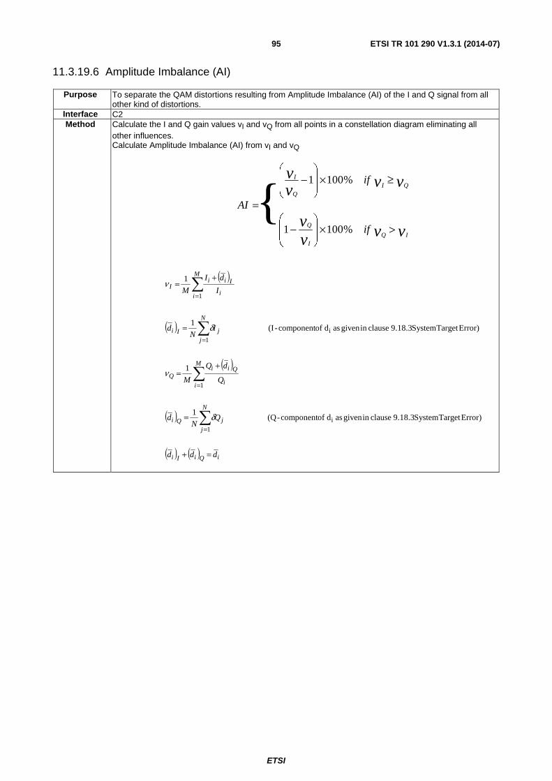
ETSI
ETSI TR 101 290 V1.3.1 (2014-07) 95
11.3.19.6 Amplitude Imbalance (AI)
Purpose To separate the QAM distortions resulting from Amplitude Imbalance (AI) of the I and Q signal from all other kind of distortions.
Interface C2 Method Calculate the I and Q gain values vI and vQ from all points in a constellation diagram eliminating all
other influences. Calculate Amplitude Imbalance (AI) from vI and vQ
vvvv
vvvv
IQI
Q
QIQ
I
if
if
AI
>×⎟⎟
⎠
⎞
⎜⎜
⎝
⎛−
≥×⎟⎟
⎠
⎞
⎜⎜
⎝
⎛−
=
%1001
%1001
{
( )
( )
( )
( )
( ) ( ) iQiIi
N
j
jQi
M
i i
QiiQ
N
j
jIi
M
i i
IiiI
ddd
QN
d
Q
dQ
M
IN
d
I
dI
M
=+
=
+=
=
+=
∑
∑
∑
∑
=
=
=
=
Error)Target System 9.18.3 clausein given as d ofcomponent -(Q 1
1
Error)Target System 9.18.3 clausein given as d ofcomponent -(I 1
1
i
1
1
i
1
1
δ
ν
δ
ν
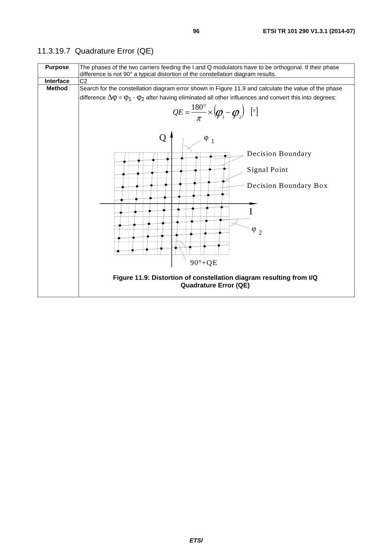
ETSI
ETSI TR 101 290 V1.3.1 (2014-07) 96
11.3.19.7 Quadrature Error (QE)
Purpose The phases of the two carriers feeding the I and Q modulators have to be orthogonal. If their phase difference is not 90° a typical distortion of the constellation diagram results.
Interface C2 Method Search for the constellation diagram error shown in Figure 11.9 and calculate the value of the phase
difference Δϕ = ϕ1 - ϕ2 after having eliminated all other influences and convert this into degrees:
( ) [ ]°−×°= ϕϕπ 21
180QE
I
Q
Decision Boundary
Signal Point
Decision Boundary Box
1ϕ
2ϕ
90°+QE
Figure 11.9: Distortion of constellation diagram resulting from I/Q Quadrature Error (QE)
ETSI
ETSI TR 101 290 V1.3.1 (2014-07) 97
11.3.20 SFN synchronization
Purpose To measure and adjust the signal delay of an OFDM transmitter to a given value so that the transmitters in an SFN can be synchronized.
Interface C1 Method Based on a sufficient number of I/Q samples, the channel response of the received DVB-T2 signal is
calculated. The measurement of the SFN synchronization depends on the location where this measurement is executed. The SFN synchronization is related to two independent parameters:
a) Time synchronization: All signals received from the certain transmitters at the location of interest should be received within the Guard Interval. It is the task of the network planning that also echoes from these signals will not infringe this rule.
Method: The complex channel impulse response is measured. In addition, the Guard Interval is indicated. Also pre-echoes are taken into account correctly, according to the positioning of the FFT window. The indication of the Guard Interval should always start with the start of the FFT window position.
b) Frequency synchronization: The center frequency of all signals received from the certain transmitters should be within a certain limit. In practice, 1 Hz has been established as a good and practicable target value for this limit in case of an 8 MHz channel and an 8k FFT size. For other channel bandwidth and other FFT sizes, e.g.16k and 32k signals, a proportionally higher accuracy may be required.
The SFN frequency offset can be calculated as a relative value. It should be referenced to the signal path that provides the maximum power. Method: The complex channel impulse response is measured from which the frequency offset of each echo is derived and indicated. Also pre-echoes have to be taken into account correctly. A positive SFN frequency offset value means that the local center frequency of the related echo is higher than the local center frequency of the reference signal.
11.3.21 L1 signalling error
Purpose The consistency of the L1 data is essential for the successful decoding of the DVB-T2 signal by the receiver.
Interface C3 Method The receiver checks the CRC within the corresponding L1-pre and L1-post data.
11.3.22 RMS Delay-Spread (RMS-DS)
Purpose The performance of OFDM based systems depends on the characteristics of the transmission channel. The extent of the multipath propagation of the transmission channel is characterized by means of the root means square (RMS) of the channel delay spread.
Interface C1 Method The RMS Delay-Spread is directly measured from the channel impulse response. It is calculated from
all i multipath components with power iP and excess delay iτ that exceed a specified power
threshold (e.g. -15 dB, -20 dB, -25 dB) with respect to the strongest component. The excess delay (or
delta) iτ is defined as the delta of the multipath component i with respect to the strongest signal
component. The calculation should be limited to the Guard Interval to avoid ambiguities.
∑
∑∑
∑=
=
=
=
=−⋅=n
ii
n
iii
d
n
idiin
ii
RMS
P
P
withP
P1
1
1
22
1
)(
)(1
τττττ
ETSI
ETSI TR 101 290 V1.3.1 (2014-07) 98
11.3.23 Maximum Excess Delay (MED)
Purpose The performance of OFDM based systems depends on the characteristics of the transmission channel. The largest multipath delay of the transmission channel is characterized by means of the Maximum Excess Delay (MED).
Interface C1 Method The Maximum Excess Delay is directly measured from the channel impulse response. It is defined as
the maximum delay maxτ of all multipath components that exceed a specified power threshold of
e.g. -15 dB, -20 dB, -25 dB with respect to the strongest component. The maximum excess delay
maxτ is defined with regard to the first arrived component above the specified power threshold.
11.3.24 Receiver Buffer Model (RBM) validation test
Purpose This test applies a test stream for an out-of-service test to the receiver to validate the proper functioning of the receiver buffer.
Interface C Method A DVB-T2 signal is applied to the input of a DVB-T2 receiver. This DVB-T2 signal contains a test
stream (e.g. V&V number 7xx). The test stream is generated (typically in the T2 gateway) and includes a modified Common PLP. The modified Common PLP for this test does not contain the tables and service information as usual, but an externally applied video/ audio test stream. The failure point is defined as ESR5. ESR (Errored Second Ratio) is defined in clause 11.2.18. One errored second during a time interval of 20 seconds is given as ESR5 (5 % of the seconds are errored).
11.3.25 Relative power level during the non-P1 part of the FEF (RLF_non_P1)
Purpose The purpose of the test is to measure the average power level of the non-P1 signal (excluding the rise time/fall time between the P1 and adjacent waveforms) of the FEF relative to the power of the T2 signal, excluding the FEF. This procedure allows for in-service measurements of co-channel interference (CCI) when empty FEFs are applied.
Interface C Method The DVB-T2 system makes it possible to broadcast a FEF part carrying a non-T2 waveform at
potentially another power level, including an empty FEF. Empty FEF means null power during non-P1 part of the FEF. A DVB-T2 signal is generated including a FEF part, which contains some other waveform than DVB-T2, e.g. T2 TX-SIG or an empty FEF. During the FEF period the power level of the non-P1 part of the FEF is measured. In addition the power level of the DVB-T2 signal (excluding the FEF part) is measured. A fast enough power sensor gated properly, or a spectrum analyser capable for channel power measurements, or a DVB-T2 receiver can be used for this measurement.
NOTE: Note that DVB-T2 receivers of the 1st generation should ignore FEFs.
12 Measurements for the second generation cable system (DVB-C2)
12.1 Introduction
The DVB-C2 system as it is addressed in the following clauses and sub-clauses, spans from the input interface (MPEG TS or GSE stream) to the output interface (RF signal) of the DVB-C2 transmitter.
NOTE: The development of DVB-C2 modulator interface is not finalized at the time of completion of these Measurement Guidelines.
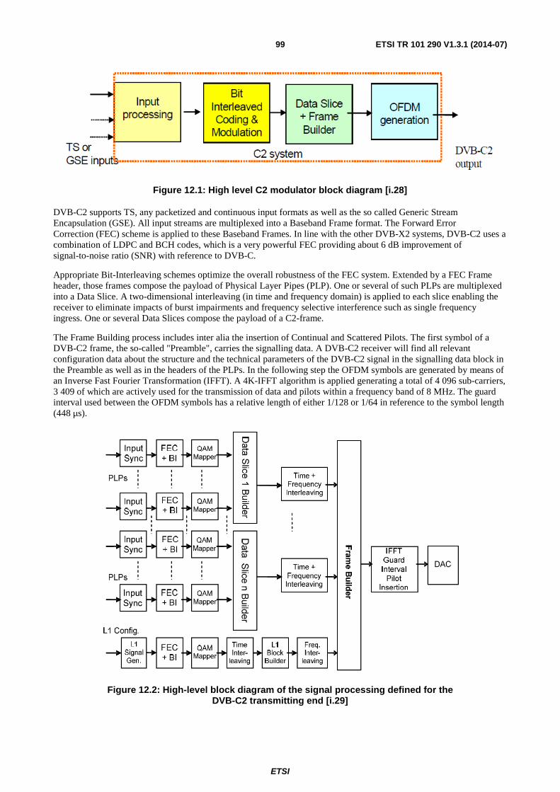
ETSI
ETSI TR 101 290 V1.3.1 (2014-07) 99
Figure 12.1: High level C2 modulator block diagram [i.28]
DVB-C2 supports TS, any packetized and continuous input formats as well as the so called Generic Stream Encapsulation (GSE). All input streams are multiplexed into a Baseband Frame format. The Forward Error Correction (FEC) scheme is applied to these Baseband Frames. In line with the other DVB-X2 systems, DVB-C2 uses a combination of LDPC and BCH codes, which is a very powerful FEC providing about 6 dB improvement of signal-to-noise ratio (SNR) with reference to DVB-C.
Appropriate Bit-Interleaving schemes optimize the overall robustness of the FEC system. Extended by a FEC Frame header, those frames compose the payload of Physical Layer Pipes (PLP). One or several of such PLPs are multiplexed into a Data Slice. A two-dimensional interleaving (in time and frequency domain) is applied to each slice enabling the receiver to eliminate impacts of burst impairments and frequency selective interference such as single frequency ingress. One or several Data Slices compose the payload of a C2-frame.
The Frame Building process includes inter alia the insertion of Continual and Scattered Pilots. The first symbol of a DVB-C2 frame, the so-called "Preamble", carries the signalling data. A DVB-C2 receiver will find all relevant configuration data about the structure and the technical parameters of the DVB-C2 signal in the signalling data block in the Preamble as well as in the headers of the PLPs. In the following step the OFDM symbols are generated by means of an Inverse Fast Fourier Transformation (IFFT). A 4K-IFFT algorithm is applied generating a total of 4 096 sub-carriers, 3 409 of which are actively used for the transmission of data and pilots within a frequency band of 8 MHz. The guard interval used between the OFDM symbols has a relative length of either 1/128 or 1/64 in reference to the symbol length (448 μs).
Figure 12.2: High-level block diagram of the signal processing defined for the DVB-C2 transmitting end [i.29]
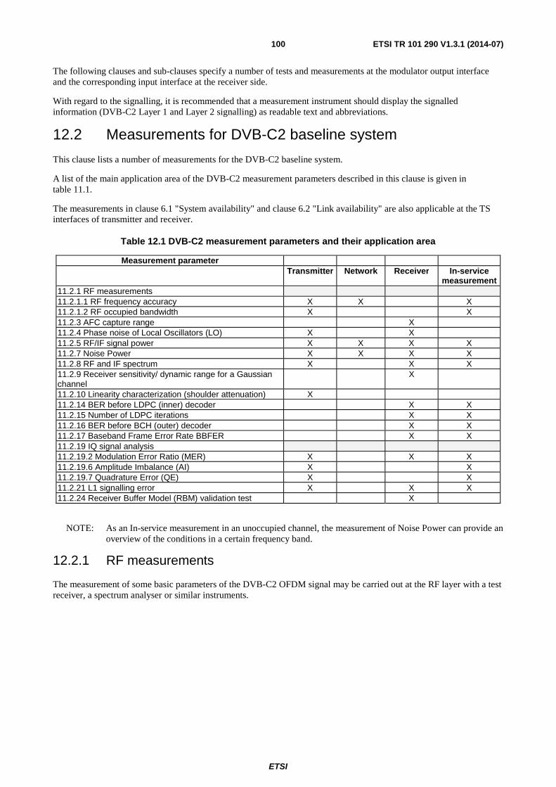
ETSI
ETSI TR 101 290 V1.3.1 (2014-07) 100
The following clauses and sub-clauses specify a number of tests and measurements at the modulator output interface and the corresponding input interface at the receiver side.
With regard to the signalling, it is recommended that a measurement instrument should display the signalled information (DVB-C2 Layer 1 and Layer 2 signalling) as readable text and abbreviations.
12.2 Measurements for DVB-C2 baseline system
This clause lists a number of measurements for the DVB-C2 baseline system.
A list of the main application area of the DVB-C2 measurement parameters described in this clause is given in table 11.1.
The measurements in clause 6.1 "System availability" and clause 6.2 "Link availability" are also applicable at the TS interfaces of transmitter and receiver.
Table 12.1 DVB-C2 measurement parameters and their application area
Measurement parameter Transmitter Network Receiver In-service
measurement 11.2.1 RF measurements 11.2.1.1 RF frequency accuracy X X X 11.2.1.2 RF occupied bandwidth X X 11.2.3 AFC capture range X 11.2.4 Phase noise of Local Oscillators (LO) X X 11.2.5 RF/IF signal power X X X X 11.2.7 Noise Power X X X X 11.2.8 RF and IF spectrum X X X 11.2.9 Receiver sensitivity/ dynamic range for a Gaussian channel
X
11.2.10 Linearity characterization (shoulder attenuation) X 11.2.14 BER before LDPC (inner) decoder X X 11.2.15 Number of LDPC iterations X X 11.2.16 BER before BCH (outer) decoder X X 11.2.17 Baseband Frame Error Rate BBFER X X 11.2.19 IQ signal analysis 11.2.19.2 Modulation Error Ratio (MER) X X X 11.2.19.6 Amplitude Imbalance (AI) X X 11.2.19.7 Quadrature Error (QE) X X 11.2.21 L1 signalling error X X X 11.2.24 Receiver Buffer Model (RBM) validation test X
NOTE: As an In-service measurement in an unoccupied channel, the measurement of Noise Power can provide an overview of the conditions in a certain frequency band.
12.2.1 RF measurements
The measurement of some basic parameters of the DVB-C2 OFDM signal may be carried out at the RF layer with a test receiver, a spectrum analyser or similar instruments.
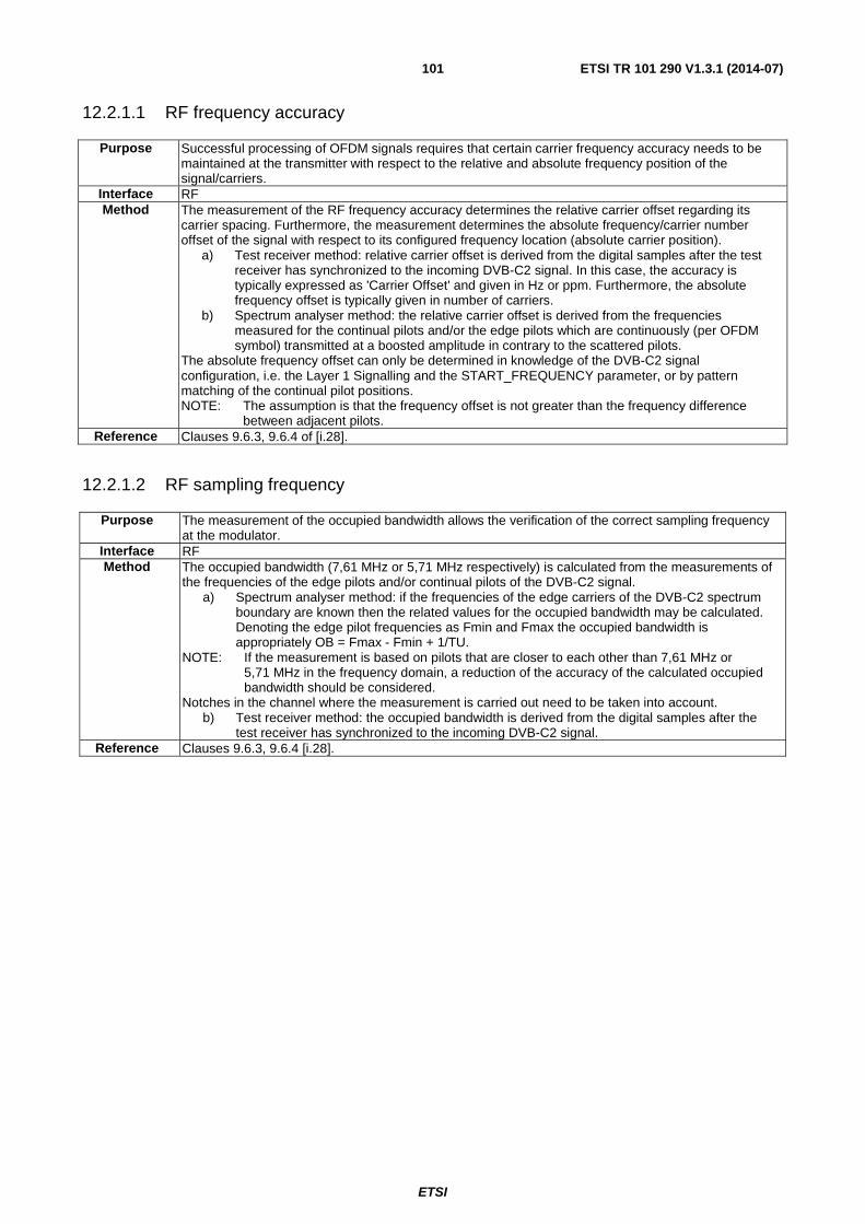
ETSI
ETSI TR 101 290 V1.3.1 (2014-07) 101
12.2.1.1 RF frequency accuracy
Purpose Successful processing of OFDM signals requires that certain carrier frequency accuracy needs to be maintained at the transmitter with respect to the relative and absolute frequency position of the signal/carriers.
Interface RF Method The measurement of the RF frequency accuracy determines the relative carrier offset regarding its
carrier spacing. Furthermore, the measurement determines the absolute frequency/carrier number offset of the signal with respect to its configured frequency location (absolute carrier position).
a) Test receiver method: relative carrier offset is derived from the digital samples after the test receiver has synchronized to the incoming DVB-C2 signal. In this case, the accuracy is typically expressed as 'Carrier Offset' and given in Hz or ppm. Furthermore, the absolute frequency offset is typically given in number of carriers.
b) Spectrum analyser method: the relative carrier offset is derived from the frequencies measured for the continual pilots and/or the edge pilots which are continuously (per OFDM symbol) transmitted at a boosted amplitude in contrary to the scattered pilots.
The absolute frequency offset can only be determined in knowledge of the DVB-C2 signal configuration, i.e. the Layer 1 Signalling and the START_FREQUENCY parameter, or by pattern matching of the continual pilot positions. NOTE: The assumption is that the frequency offset is not greater than the frequency difference
between adjacent pilots. Reference Clauses 9.6.3, 9.6.4 of [i.28].
12.2.1.2 RF sampling frequency
Purpose The measurement of the occupied bandwidth allows the verification of the correct sampling frequency at the modulator.
Interface RF Method The occupied bandwidth (7,61 MHz or 5,71 MHz respectively) is calculated from the measurements of
the frequencies of the edge pilots and/or continual pilots of the DVB-C2 signal. a) Spectrum analyser method: if the frequencies of the edge carriers of the DVB-C2 spectrum
boundary are known then the related values for the occupied bandwidth may be calculated. Denoting the edge pilot frequencies as Fmin and Fmax the occupied bandwidth is appropriately OB = Fmax - Fmin + 1/TU.
NOTE: If the measurement is based on pilots that are closer to each other than 7,61 MHz or 5,71 MHz in the frequency domain, a reduction of the accuracy of the calculated occupied bandwidth should be considered.
Notches in the channel where the measurement is carried out need to be taken into account. b) Test receiver method: the occupied bandwidth is derived from the digital samples after the
test receiver has synchronized to the incoming DVB-C2 signal. Reference Clauses 9.6.3, 9.6.4 [i.28].
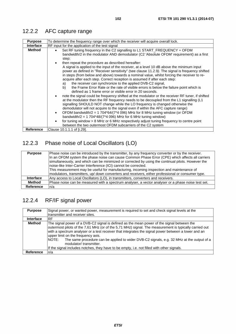
ETSI
ETSI TR 101 290 V1.3.1 (2014-07) 102
12.2.2 AFC capture range
Purpose To determine the frequency range over which the receiver will acquire overall lock. Interface RF input for the application of the test signal Method • Set RF tuning frequency in the C2 signalling to L1 START_FREQUENCY + OFDM
bandwidth/2 in the modulator AND demodulator (C2 'Absolute OFDM' requirement) as a first step;
• then repeat the procedure as described hereafter: A signal is applied to the input of the receiver, at a level 10 dB above the minimum input
power as defined in "Receiver sensitivity" (see clause 11.2.9). The signal is frequency shifted in steps (from below and above) towards a nominal value, whilst forcing the receiver to re-acquire after each step. Correct reception is assumed if after each step: a) the receiver can synchronize to the applied DVB-C2 signal, b) the Frame Error Rate or the rate of visible errors is below the failure point which is
defined as 1 frame error or visible error in 20 seconds. • note the signal could be frequency shifted at the modulator or the receiver RF tuner, if shifted
at the modulator then the RF frequency needs to be decoupled from the L1 signalling (L1 signalling SHOULD NOT change while the LO frequency is changed otherwise the demodulator will not acquire to the signal even if within the AFC capture range)
• OFDM bandwidth/2 = 1 704*64/(7*4 096) MHz for 8 MHz tuning window (or OFDM bandwidth/2 = 1 704*48/(7*4 096) MHz for 6 MHz tuning window)
• for tuning window > 8 MHz or 6 MHz respectively adjust tuning frequency to centre point between the two outermost OFDM subcarriers of the C2 system
Reference Clause 10.1.1.1 of [i.29].
12.2.3 Phase noise of Local Oscillators (LO)
Purpose Phase noise can be introduced by the transmitter, by any frequency converter or by the receiver. In an OFDM system the phase noise can cause Common Phase Error (CPE) which affects all carriers simultaneously, and which can be minimized or corrected by using the continual pilots. However the noise-like Inter-Carrier Interference (ICI) cannot be corrected. This measurement may be useful for manufacturing, incoming inspection and maintenance of modulators, transmitters, up/ down converters and receivers, either professional or consumer type.
Interface Any access to Local Oscillators (LO), in transmitters, converters and receivers. Method Phase noise can be measured with a spectrum analyser, a vector analyser or a phase noise test set.
Reference n/a
12.2.4 RF/IF signal power
Purpose Signal power, or wanted power, measurement is required to set and check signal levels at the transmitter and receiver sites.
Interface RF Method The signal power of a DVB-C2 signal is defined as the mean power of the signal between the
outermost pilots of the 7,61 MHz (or of the 5,71 MHz) signal. The measurement is typically carried out with a spectrum analyser or a test receiver that integrates the signal power between a lower and an upper limit on the frequency axis. NOTE: The same procedure can be applied to wider DVB-C2 signals, e.g. 32 MHz at the output of a
modulator/ transmitter. If the signal includes notches, they have to be empty, i.e. not filled with other signals.
Reference n/a
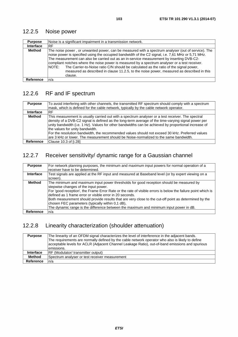
ETSI
ETSI TR 101 290 V1.3.1 (2014-07) 103
12.2.5 Noise power
Purpose Noise is a significant impairment in a transmission network. Interface RF Method The noise power , or unwanted power, can be measured with a spectrum analyser (out of service). The
noise power is specified using the occupied bandwidth of the C2 signal, i.e. 7,61 MHz or 5,71 MHz. The measurement can also be carried out as an in-service measurement by inserting DVB-C2-compliant notches where the noise power is measured by a spectrum analyser or a test receiver. NOTE: The Carrier-to-Noise ratio C/N should be calculated as the ratio of the signal power,
measured as described in clause 11.2.5, to the noise power, measured as described in this clause.
Reference n/a
12.2.6 RF and IF spectrum
Purpose To avoid interfering with other channels, the transmitted RF spectrum should comply with a spectrum mask, which is defined for the cable network, typically by the cable network operator.
Interface RF Method This measurement is usually carried out with a spectrum analyser or a test receiver. The spectral
density of a DVB-C2 signal is defined as the long-term average of the time-varying signal power per unity bandwidth (i.e. 1 Hz). Values for other bandwidths can be achieved by proportional increase of the values for unity bandwidth. For the resolution bandwidth, the recommended values should not exceed 30 kHz. Preferred values are 3 kHz or lower. The measurement should be Noise-normalized to the same bandwidth.
Reference Clause 10.3 of [i.28]
12.2.7 Receiver sensitivity/ dynamic range for a Gaussian channel
Purpose For network planning purposes, the minimum and maximum input powers for normal operation of a receiver have to be determined.
Interface Test signals are applied at the RF input and measured at Baseband level (or by expert viewing on a screen).
Method The minimum and maximum input power thresholds for good reception should be measured by stepwise changes of the input power. For 'good reception', the Frame Error Rate or the rate of visible errors is below the failure point which is defined as 1 frame error or visible error in 20 seconds. Both measurement should provide results that are very close to the cut-off point as determined by the chosen FEC parameters (typically within 0,1 dB), The dynamic range is the difference between the maximum and minimum input power in dB.
Reference n/a
12.2.8 Linearity characterization (shoulder attenuation)
Purpose The linearity of an OFDM signal characterizes the level of interference in the adjacent bands. The requirements are normally defined by the cable network operator who also is likely to define acceptable levels for ACLR (Adjacent Channel Leakage Ratio), out-of-band emissions and spurious emissions.
Interface RF (Modulator/ transmitter output) Method Spectrum analyser or test receiver measurement
Reference n/a
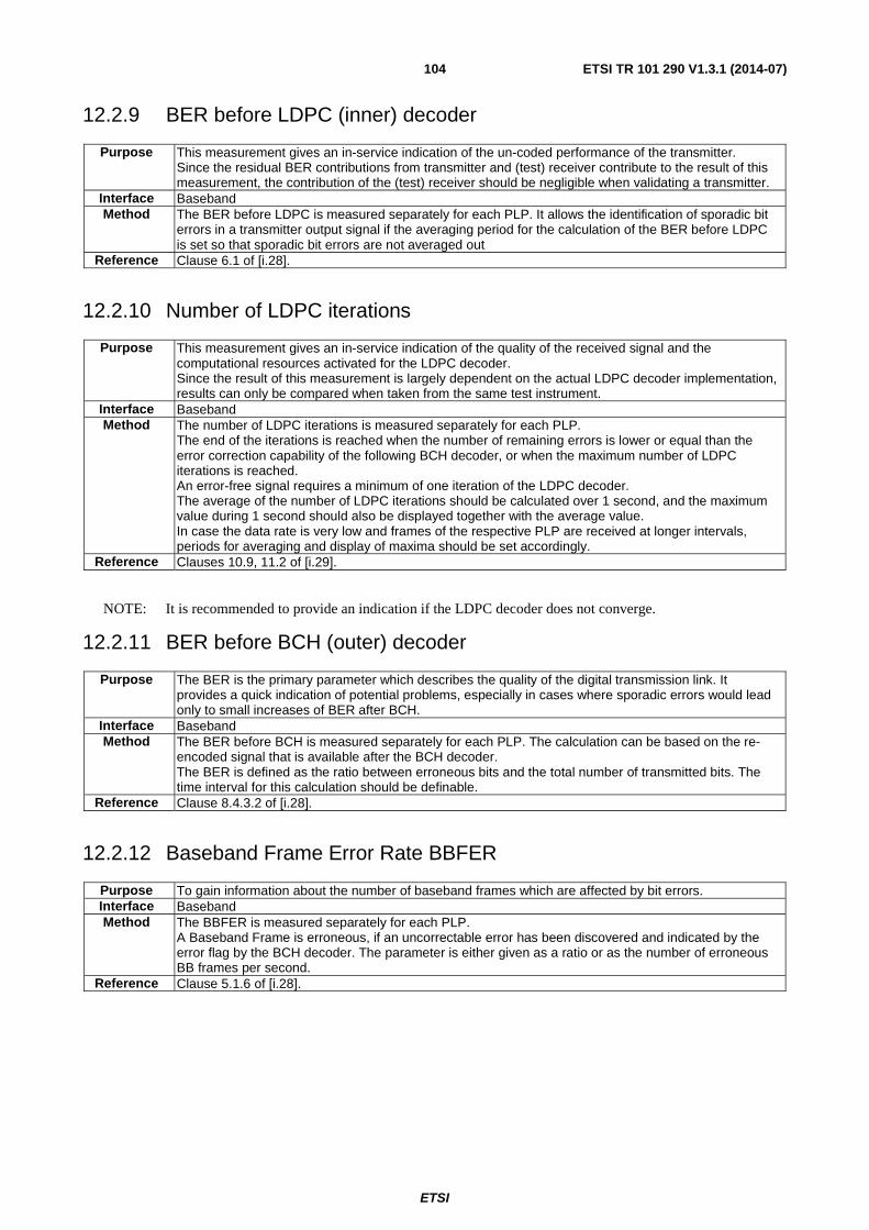
ETSI
ETSI TR 101 290 V1.3.1 (2014-07) 104
12.2.9 BER before LDPC (inner) decoder
Purpose This measurement gives an in-service indication of the un-coded performance of the transmitter. Since the residual BER contributions from transmitter and (test) receiver contribute to the result of this measurement, the contribution of the (test) receiver should be negligible when validating a transmitter.
Interface Baseband Method The BER before LDPC is measured separately for each PLP. It allows the identification of sporadic bit
errors in a transmitter output signal if the averaging period for the calculation of the BER before LDPC is set so that sporadic bit errors are not averaged out
Reference Clause 6.1 of [i.28].
12.2.10 Number of LDPC iterations
Purpose This measurement gives an in-service indication of the quality of the received signal and the computational resources activated for the LDPC decoder. Since the result of this measurement is largely dependent on the actual LDPC decoder implementation, results can only be compared when taken from the same test instrument.
Interface Baseband Method The number of LDPC iterations is measured separately for each PLP.
The end of the iterations is reached when the number of remaining errors is lower or equal than the error correction capability of the following BCH decoder, or when the maximum number of LDPC iterations is reached. An error-free signal requires a minimum of one iteration of the LDPC decoder. The average of the number of LDPC iterations should be calculated over 1 second, and the maximum value during 1 second should also be displayed together with the average value. In case the data rate is very low and frames of the respective PLP are received at longer intervals, periods for averaging and display of maxima should be set accordingly.
Reference Clauses 10.9, 11.2 of [i.29].
NOTE: It is recommended to provide an indication if the LDPC decoder does not converge.
12.2.11 BER before BCH (outer) decoder
Purpose The BER is the primary parameter which describes the quality of the digital transmission link. It provides a quick indication of potential problems, especially in cases where sporadic errors would lead only to small increases of BER after BCH.
Interface Baseband Method The BER before BCH is measured separately for each PLP. The calculation can be based on the re-
encoded signal that is available after the BCH decoder. The BER is defined as the ratio between erroneous bits and the total number of transmitted bits. The time interval for this calculation should be definable.
Reference Clause 8.4.3.2 of [i.28].
12.2.12 Baseband Frame Error Rate BBFER
Purpose To gain information about the number of baseband frames which are affected by bit errors. Interface Baseband Method The BBFER is measured separately for each PLP.
A Baseband Frame is erroneous, if an uncorrectable error has been discovered and indicated by the error flag by the BCH decoder. The parameter is either given as a ratio or as the number of erroneous BB frames per second.
Reference Clause 5.1.6 of [i.28].
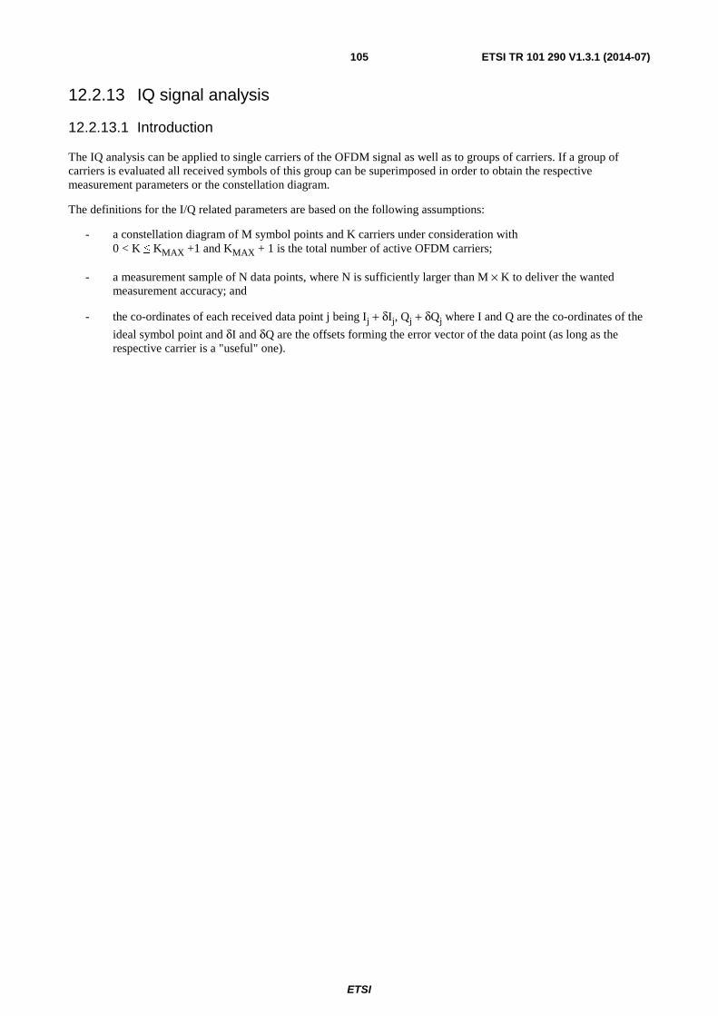
ETSI
ETSI TR 101 290 V1.3.1 (2014-07) 105
12.2.13 IQ signal analysis
12.2.13.1 Introduction
The IQ analysis can be applied to single carriers of the OFDM signal as well as to groups of carriers. If a group of carriers is evaluated all received symbols of this group can be superimposed in order to obtain the respective measurement parameters or the constellation diagram.
The definitions for the I/Q related parameters are based on the following assumptions:
- a constellation diagram of M symbol points and K carriers under consideration with 0 < K ≤ KMAX +1 and KMAX + 1 is the total number of active OFDM carriers;
- a measurement sample of N data points, where N is sufficiently larger than M × K to deliver the wanted measurement accuracy; and
- the co-ordinates of each received data point j being Ij + δIj, Qj + δQj where I and Q are the co-ordinates of the
ideal symbol point and δI and δQ are the offsets forming the error vector of the data point (as long as the respective carrier is a "useful" one).
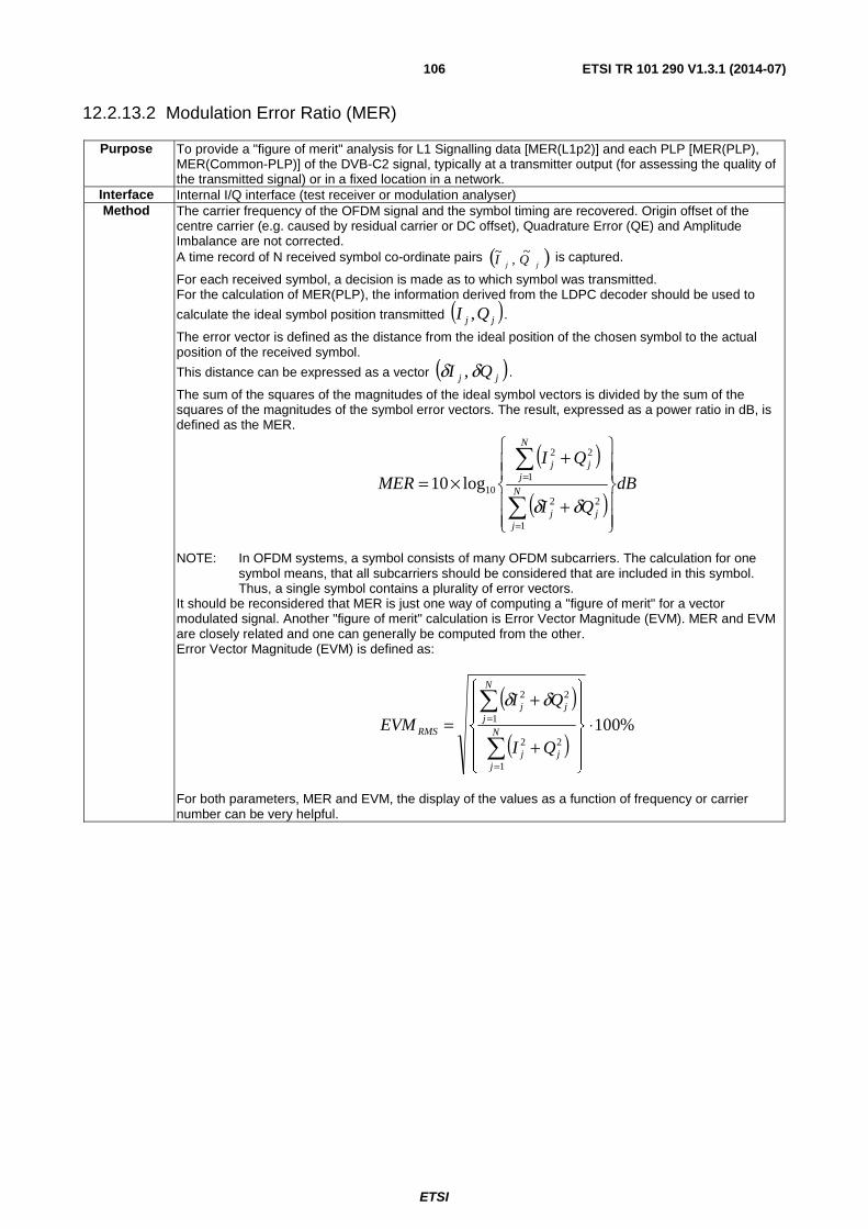
ETSI
ETSI TR 101 290 V1.3.1 (2014-07) 106
12.2.13.2 Modulation Error Ratio (MER)
Purpose To provide a "figure of merit" analysis for L1 Signalling data [MER(L1p2)] and each PLP [MER(PLP), MER(Common-PLP)] of the DVB-C2 signal, typically at a transmitter output (for assessing the quality of the transmitted signal) or in a fixed location in a network.
Interface Internal I/Q interface (test receiver or modulation analyser) Method The carrier frequency of the OFDM signal and the symbol timing are recovered. Origin offset of the
centre carrier (e.g. caused by residual carrier or DC offset), Quadrature Error (QE) and Amplitude Imbalance are not corrected. A time record of N received symbol co-ordinate pairs ( )jj QI
~,
~ is captured.
For each received symbol, a decision is made as to which symbol was transmitted. For the calculation of MER(PLP), the information derived from the LDPC decoder should be used to
calculate the ideal symbol position transmitted ( )jj QI , .
The error vector is defined as the distance from the ideal position of the chosen symbol to the actual position of the received symbol.
This distance can be expressed as a vector ( )jj QI δδ , .
The sum of the squares of the magnitudes of the ideal symbol vectors is divided by the sum of the squares of the magnitudes of the symbol error vectors. The result, expressed as a power ratio in dB, is defined as the MER.
( )
( )dB
QI
QI
MER N
jjj
N
jjj
⎪⎪
⎭
⎪⎪
⎬
⎫
⎪⎪
⎩
⎪⎪
⎨
⎧
+
+×=
∑
∑
=
=
1
22
1
22
10log10δδ
NOTE: In OFDM systems, a symbol consists of many OFDM subcarriers. The calculation for one symbol means, that all subcarriers should be considered that are included in this symbol. Thus, a single symbol contains a plurality of error vectors.
It should be reconsidered that MER is just one way of computing a "figure of merit" for a vector modulated signal. Another "figure of merit" calculation is Error Vector Magnitude (EVM). MER and EVM are closely related and one can generally be computed from the other. Error Vector Magnitude (EVM) is defined as:
( )
( )%100
1
22
1
22
⋅
⎪⎪
⎭
⎪⎪
⎬
⎫
⎪⎪
⎩
⎪⎪
⎨
⎧
+
+=
∑
∑
=
=N
jjj
N
jjj
RMS
QI
QI
EVM
δδ
For both parameters, MER and EVM, the display of the values as a function of frequency or carrier number can be very helpful.
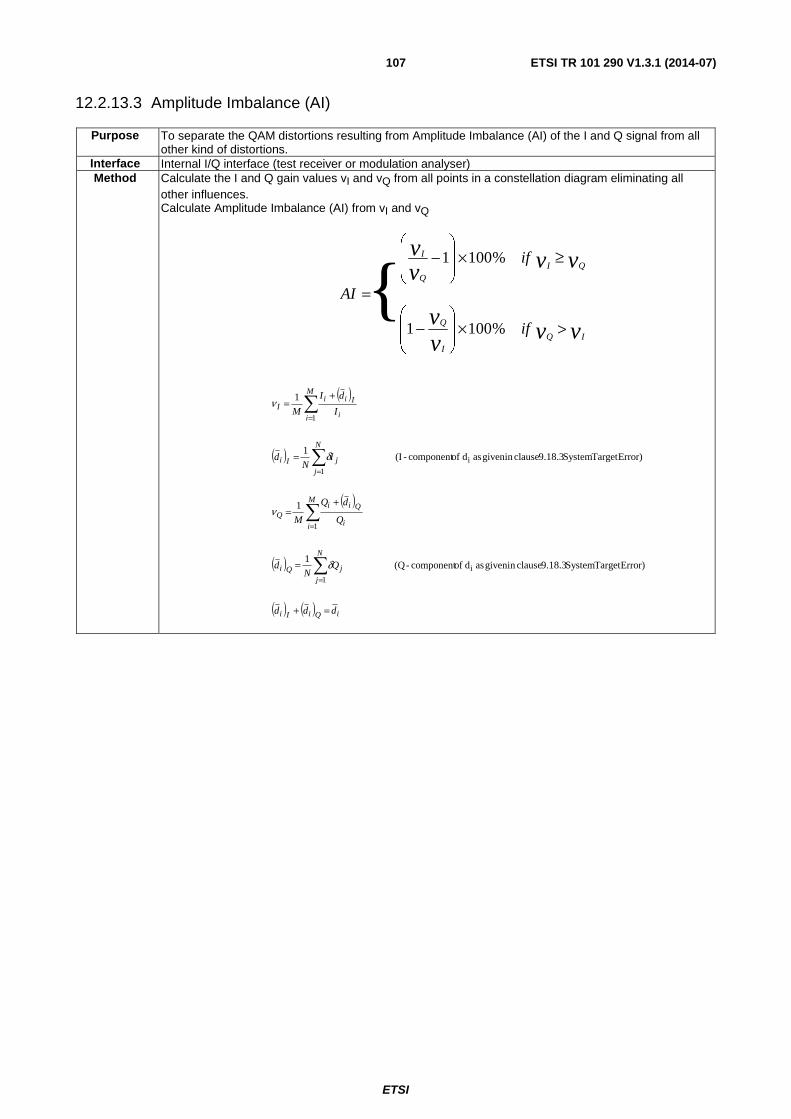
ETSI
ETSI TR 101 290 V1.3.1 (2014-07) 107
12.2.13.3 Amplitude Imbalance (AI)
Purpose To separate the QAM distortions resulting from Amplitude Imbalance (AI) of the I and Q signal from all other kind of distortions.
Interface Internal I/Q interface (test receiver or modulation analyser) Method Calculate the I and Q gain values vI and vQ from all points in a constellation diagram eliminating all
other influences. Calculate Amplitude Imbalance (AI) from vI and vQ
vvvv
vvvv
IQI
Q
QIQ
I
if
if
AI
>×⎟⎟
⎠
⎞
⎜⎜
⎝
⎛−
≥×⎟⎟
⎠
⎞
⎜⎜
⎝
⎛−
=
%1001
%1001
{
( )
( )
( )
( )
( ) ( ) iQiIi
N
j
jQi
M
i i
QiiQ
N
j
jIi
M
i i
IiiI
ddd
QN
d
Q
dQ
M
IN
d
I
dI
M
=+
=
+=
=
+=
∑
∑
∑
∑
=
=
=
=
Error)Target System 9.18.3 clausein given as d ofcomponent -(Q 1
1
Error)Target System 9.18.3 clausein given as d ofcomponent -(I 1
1
i
1
1
i
1
1
δ
ν
δ
ν
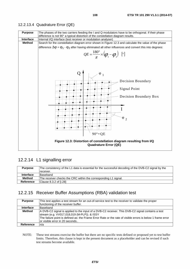
ETSI
ETSI TR 101 290 V1.3.1 (2014-07) 108
12.2.13.4 Quadrature Error (QE)
Purpose The phases of the two carriers feeding the I and Q modulators have to be orthogonal. If their phase difference is not 90° a typical distortion of the constellation diagram results.
Interface Internal I/Q interface (test receiver or modulation analyser) Method Search for the constellation diagram error shown in Figure 12.3 and calculate the value of the phase
difference Δϕ = ϕ1 - ϕ2 after having eliminated all other influences and convert this into degrees:
( ) [ ]°−×°= ϕϕπ 21
180QE
I
Q
Decision Boundary
Signal Point
Decision Boundary Box
1ϕ
2ϕ
90°+QE
Figure 12.3: Distortion of constellation diagram resulting from I/Q Quadrature Error (QE)
12.2.14 L1 signalling error
Purpose The consistency of the L1 data is essential for the successful decoding of the DVB-C2 signal by the receiver.
Interface Baseband Method The receiver checks the CRC within the corresponding L1 signal.
Reference Clause 8.3.2 of [i.28]
12.2.15 Receiver Buffer Assumptions (RBA) validation test
Purpose This test applies a test stream for an out-of-service test to the receiver to validate the proper functioning of the receiver buffer.
Interface Baseband Method A DVB-C2 signal is applied to the input of a DVB-C2 receiver. This DVB-C2 signal contains a test
stream (e.g. VV017,018,019 (M-PLP)). & ISSY The failure point is defined as: the Frame Error Rate or the rate of visible errors is below 1 frame error or visible error in 20 seconds..
Reference n/a
NOTE: These test streams exercise the buffer but there are no specific tests defined or proposed yet to test buffer limits. Therefore, this clause is kept in the present document as a placeholder and can be revised if such test streams become available.

ETSI
ETSI TR 101 290 V1.3.1 (2014-07) 109
Annex A: General measurement methods
A.1 Introduction It is recommended that manufacturers add the test mode described in this annex to certain professional grade cable and satellite broadcast equipment. This recommendation is relevant to equipment that implements the channel encoding schemes defined in EN 300 429 [i.6] (cable) and EN 300 421 [i.5] (satellite).
The purpose of the recommended test mode is to simplify out of service testing of systems and system components by making the channel encoder able to generate a known, fixed, repeating bit sequence of an essentially pseudo-random nature.
The central requirement is that when the channel encoder is in the test mode, the data entering the sync inversion/randomization function is a continuous repetition of one fixed TS packet. The fixed packet is defined as the four byte sequence 0x47, 0x1f, 0xff, 0x10, followed by 184 zero bytes (0 x 00). This form of data is a refinement of the null TS packet definition in ISO/IEC 13818-1 [i.1].
A.2 Null packet definition This clause summarizes the null packet definition from ISO/IEC 13818-1 [i.1] and then describes how the definition has been extended for the purpose of the recommended test mode.
ISO/IEC 13818-1 [i.1] defines a null TS packet for the purposes of data rate stuffing.
Table A.1 shows the structure of a null TS packet using the method of describing bit stream syntax defined in clause 2.4.3.3 of ISO/IEC 13818-1 [i.1].
This description is derived from tables 2-3 Transport Header (TH) in ISO/IEC 13818-1 [i.1]. The abbreviation "bslbf" means "bit string, left bit first", and "uimsbf" means "unsigned integer, most significant bit first".
The column titled "Value", gives the bit sequence for the recommended null packet.
A null packet is defined by ISO/IEC 13818-1 [i.1] as having:
- payload_unit_start_indicator = "0";
- PID = 0x1FFF;
- transport_scrambling_control = "00";
- adaptation_field_control value = "01". This corresponds to the case "no adaptation field, payload only".
The remaining fields in the null packet that should be defined for testing purposes are:
- transport_error_indicator which is "0" unless the packet is corrupted. For testing purposes this bit is defined as "0" when the packet is generated;
- transport_priority which is not defined by ISO/IEC 13818-1 [i.1] for a null packet. For testing purposes this bit is defined as "0";
- continuity_counter which ISO/IEC 13818-1 [i.1] states is undefined for a null packet. For testing purposes this bit field is defined as "0000";
- data_byte which ISO/IEC 13818-1 [i.1] states may have any value in a null packet. For testing purposes this bit field is defined as "00000000".

ETSI
ETSI TR 101 290 V1.3.1 (2014-07) 110
Table A.1: Null TS packet definition
Syntax No. of bits Identifier Value null_transport_packet(){ sync_byte 8 bslbf "01000111" transport_error_indicator 1 bslbf "0" payload_unit_start_indicator 1 bslbf "0" transport_priority 1 bslbf "0" PID 13 uimsbf "1111111111111" transport_scrambling_control 2 bslbf "00" adaptation_field_control 2 bslbf "01" continuity_counter 4 uimsbf "0000" for (I = 0;i<N;i++) { data_byte 8 bslbf "00000000" } }
A.3 Description of the procedure for "Estimated Noise Margin" by applying statistical analysis on the constellation data
Instead of adding real noise to the received signal this method uses statistical analysis and an iterative search algorithm to estimate the added noise power to reach the critical BER.
1) Demodulate the signal to produce a statistically significant sequence of data records. Each record represents the state of the demodulated I and Q components at a decision instant.
2) Compute the average noise power as the mean square of the error vectors and calculate the estimated Savg/Navg
ratio.
( )
( )⎟⎟⎟⎟⎟⎟⎟
⎠
⎞
⎜⎜⎜⎜⎜⎜⎜
⎝
⎛
+
+
×=
∑
∑
=
=N
j
jjN
N
j
jjN
QI
QI
SNR
1
221
1
221
10log10
σσ
The σIj and σQj are the error vector co-ordinates which represent the offset from the co-ordinates of the centre (mean
value) of the actual received data for a specific constellation point, to the actual received data point j.
If only Gussian noise is present as an impairment the "centre (mean value) of the actual received data for a specific constellation point" is identical to the ideal symbol point.
N is the number of data points in the measurement sample.
3) Compute the additional noise power Nstep required to degrade the computed SNR by a certain amount. The
value Nstep is usually determined by the iterative optimization procedure which is used.
4) For each data record in the sample compute the distances d from the true position of the signal at the decision instant to each of the decision boundaries with adjacent cells. For each of the directions +I, -I, +Q, -Q that would cause a symbol error, convert the distance to the decision boundary into the number of standard deviations (k) of a normal distribution with a variance corresponding to the added noise power. The variance of the added noise power is:
stepN=2σ
and the normalized standard deviation corresponding to the distance dI+ is for example:
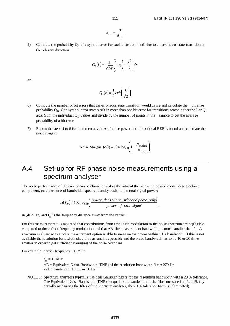
ETSI
ETSI TR 101 290 V1.3.1 (2014-07) 111
++ =
II d
kσ
5) Compute the probability QS of a symbol error for each distribution tail due to an erroneous state transition in
the relevant direction.
( ) ∫∞
⎟⎟
⎠
⎞
⎜⎜
⎝
⎛−=
k
s dxx
kQ2
exp2
1 2
π
or
( ) ⎟⎟⎠
⎞⎜⎜⎝
⎛=
22
1 kerfckQs
6) Compute the number of bit errors that the erroneous state transition would cause and calculate the bit error probability QB. One symbol error may result in more than one bit error for transitions across either the I or Q
axis. Sum the individual QB values and divide by the number of points in the sample to get the average
probability of a bit error.
7) Repeat the steps 4 to 6 for incremental values of noise power until the critical BER is found and calculate the noise margin:
Noise Margin ⎟⎟
⎠
⎞
⎜⎜
⎝
⎛+×=
avg
added
N
NdB 1log10)( 10
A.4 Set-up for RF phase noise measurements using a spectrum analyser
The noise performance of the carrier can be characterized as the ratio of the measured power in one noise sideband component, on a per hertz of bandwidth spectral density basis, to the total signal power:
( ) ⎟⎟⎠
⎞⎜⎜⎝
⎛×=
lotal_signapower_of_t
se_only)deband,phaity(one_sipower_densfm 10log10α
in (dBc/Hz) and fm is the frequency distance away from the carrier.
For this measurement it is assumed that contributions from amplitude modulation to the noise spectrum are negligible compared to those from frequency modulation and that ΔB, the measurement bandwidth, is much smaller than fm. A
spectrum analyser with a noise measurement option is able to measure the power within 1 Hz bandwidth. If this is not available the resolution bandwidth should be as small as possible and the video bandwidth has to be 10 or 20 times smaller in order to get sufficient averaging of the noise over time.
For example: carrier frequency: 36 MHz
fm = 10 kHz
ΔB = Equivalent Noise Bandwidth (ENB) of the resolution bandwidth filter: 270 Hz video bandwidth: 10 Hz or 30 Hz
NOTE 1: Spectrum analysers typically use near Gaussian filters for the resolution bandwidth with a 20 % tolerance. The Equivalent Noise Bandwidth (ENB) is equal to the bandwidth of the filter measured at -3,4 dB, (by actually measuring the filter of the spectrum analyser, the 20 % tolerance factor is eliminated).
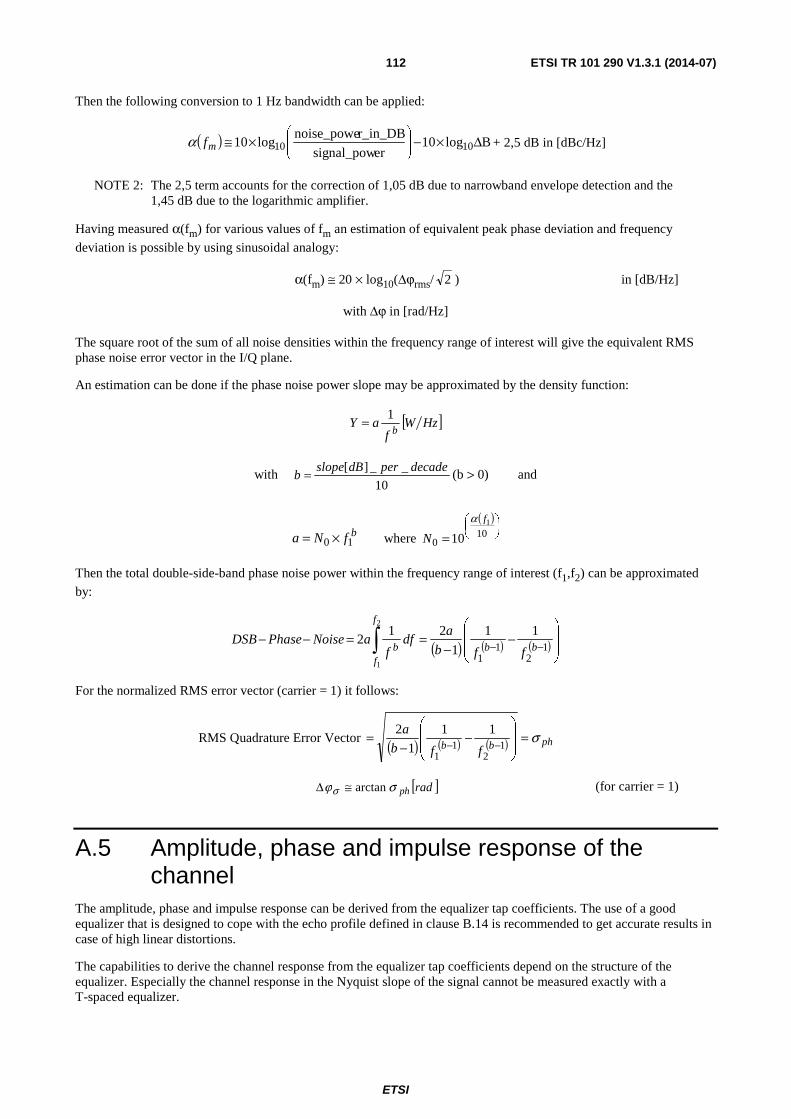
ETSI
ETSI TR 101 290 V1.3.1 (2014-07) 112
Then the following conversion to 1 Hz bandwidth can be applied:
( ) Blog10ersignal_pow
r_in_DBnoise_powelog10 1010 Δ×−⎟⎟
⎠
⎞⎜⎜⎝
⎛×≅mfα + 2,5 dB in [dBc/Hz]
NOTE 2: The 2,5 term accounts for the correction of 1,05 dB due to narrowband envelope detection and the 1,45 dB due to the logarithmic amplifier.
Having measured α(fm) for various values of fm an estimation of equivalent peak phase deviation and frequency
deviation is possible by using sinusoidal analogy:
α(fm) ≅ 20 × log10(Δϕrms/ 2 ) in [dB/Hz]
with Δϕ in [rad/Hz]
The square root of the sum of all noise densities within the frequency range of interest will give the equivalent RMS phase noise error vector in the I/Q plane.
An estimation can be done if the phase noise power slope may be approximated by the density function:
[ ]HzWf
aYb
1=
with 10
__][ decadeperdBslopeb = (b > 0) and
bfNa 10 ×= where
( )⎟⎠
⎞⎜⎝
⎛
= 100
1
10
f
N
α
Then the total double-side-band phase noise power within the frequency range of interest (f1,f2) can be approximated
by:
( ) ( ) ( )∫ ⎟⎟
⎠
⎞
⎜⎜
⎝
⎛−
−==−− −−
2
1
12
11
11
1
212
f
fbbb ffb
adf
faNoisePhaseDSB
For the normalized RMS error vector (carrier = 1) it follows:
RMS Quadrature Error Vector ( ) ( ) ( ) phbb ffb
a σ=⎟⎟
⎠
⎞
⎜⎜
⎝
⎛−
−= −− 1
21
1
11
1
2
[ ]radphσϕσ arctan≅Δ (for carrier = 1)
A.5 Amplitude, phase and impulse response of the channel
The amplitude, phase and impulse response can be derived from the equalizer tap coefficients. The use of a good equalizer that is designed to cope with the echo profile defined in clause B.14 is recommended to get accurate results in case of high linear distortions.
The capabilities to derive the channel response from the equalizer tap coefficients depend on the structure of the equalizer. Especially the channel response in the Nyquist slope of the signal cannot be measured exactly with a T-spaced equalizer.

ETSI
ETSI TR 101 290 V1.3.1 (2014-07) 113
A.6 Out of band emissions The out of band emissions can be measured using a spectrum analyser. The resolution bandwidth should be low enough to detect peaks in the out of band spectrum. The video filter should be at least 10 times lower than the resolution bandwidth for sufficient averaging of the noise-like signal.
Figure A.1: Spectrum mask as defined in EN 300 429 [i.6]

ETSI
ETSI TR 101 290 V1.3.1 (2014-07) 114
Annex B: Examples for test set-ups for satellite and cable systems Even if not demonstrated in the diagrams of this clause and also not mentioned in the explanations the receiver may be a part of the measurement device. In this case all the interfaces defined in figure 4.2 are internal ones, where the measurement device has access to.
B.1 System availability See clause 6.1.
Because this measurement is based on the error_indicator_flag in the TS header set in any previous stage including the last stage of the transmission chain the signal at interface Z should be used.
Figure B.1: Test set-up for system availability
B.2 Link availability See clause 6.2.
This measurement monitors the performance of an individual link. Therefore the RS information should be created and be correct at the start point of the link. The measurement set-up may rely on the overload information coming from the RS decoder in the receiver at interface X or on the transport_error_indicator in the header of the TS packets at interface Z.
Figure B.2: Test set-up for link availability
B.3 BER before RS See clause 6.3.
The measurement can be done as out service measurement or as in service measurement. In both cases the measurement time is an important parameter. This parameter should be selectable within a wide range by the user. Preferably the measurement should display the BER as a function of measurement time.
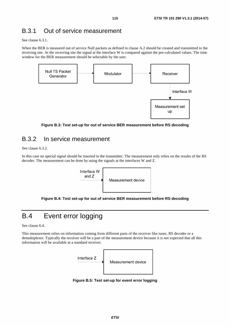
ETSI
ETSI TR 101 290 V1.3.1 (2014-07) 115
B.3.1 Out of service measurement See clause 6.3.1.
When the BER is measured out of service Null packets as defined in clause A.2 should be created and transmitted to the receiving site. At the receiving site the signal at the interface W is compared against the pre-calculated values. The time window for the BER measurement should be selectable by the user.
Figure B.3: Test set-up for out of service BER measurement before RS decoding
B.3.2 In service measurement See clause 6.3.2.
In this case no special signal should be inserted in the transmitter. The measurement only relies on the results of the RS decoder. The measurement can be done by using the signals at the interfaces W and Z.
Figure B.4: Test set-up for out of service BER measurement before RS decoding
B.4 Event error logging See clause 6.4.
This measurement relies on information coming from different parts of the receiver like tuner, RS decoder or a demultiplexer. Typically the receiver will be a part of the measurement device because it is not expected that all this information will be available at a standard receiver.
Figure B.5: Test set-up for event error logging
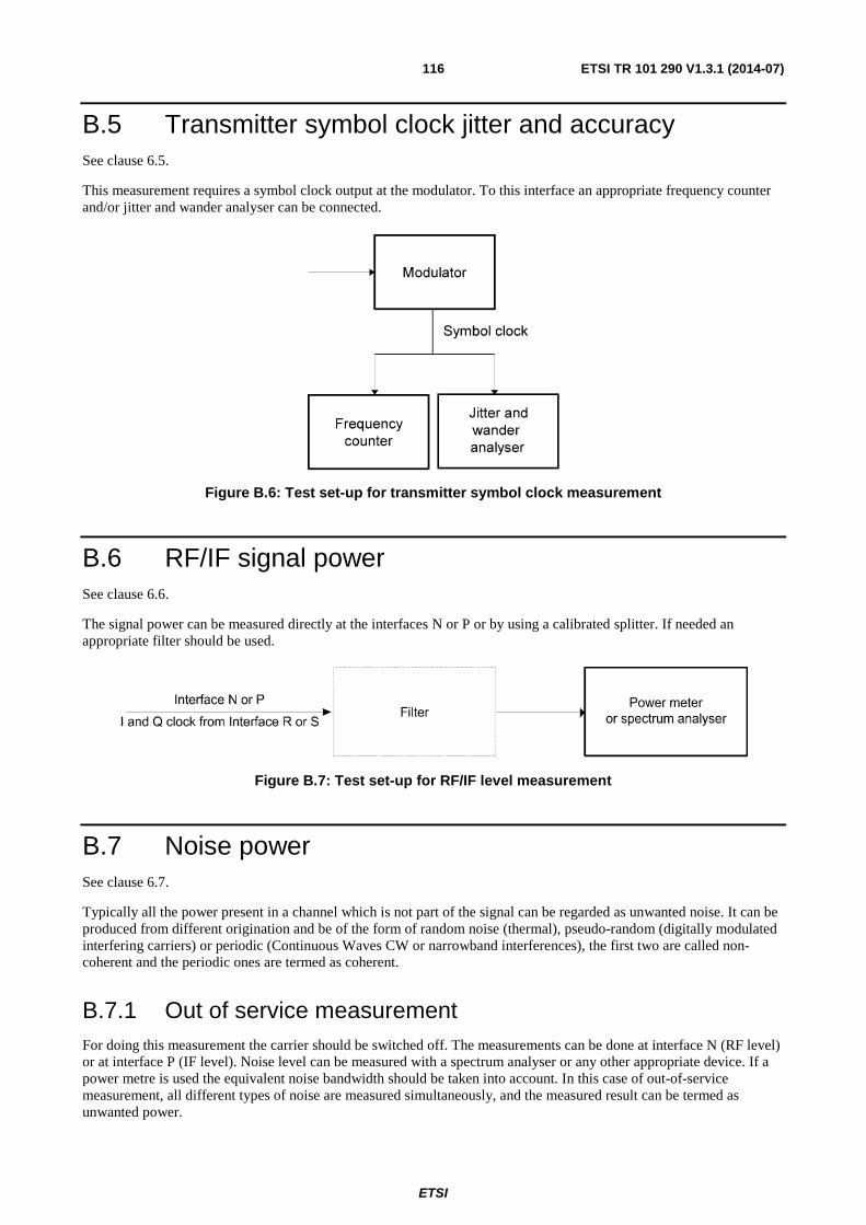
ETSI
ETSI TR 101 290 V1.3.1 (2014-07) 116
B.5 Transmitter symbol clock jitter and accuracy See clause 6.5.
This measurement requires a symbol clock output at the modulator. To this interface an appropriate frequency counter and/or jitter and wander analyser can be connected.
Figure B.6: Test set-up for transmitter symbol clock measurement
B.6 RF/IF signal power See clause 6.6.
The signal power can be measured directly at the interfaces N or P or by using a calibrated splitter. If needed an appropriate filter should be used.
Figure B.7: Test set-up for RF/IF level measurement
B.7 Noise power See clause 6.7.
Typically all the power present in a channel which is not part of the signal can be regarded as unwanted noise. It can be produced from different origination and be of the form of random noise (thermal), pseudo-random (digitally modulated interfering carriers) or periodic (Continuous Waves CW or narrowband interferences), the first two are called non-coherent and the periodic ones are termed as coherent.
B.7.1 Out of service measurement For doing this measurement the carrier should be switched off. The measurements can be done at interface N (RF level) or at interface P (IF level). Noise level can be measured with a spectrum analyser or any other appropriate device. If a power metre is used the equivalent noise bandwidth should be taken into account. In this case of out-of-service measurement, all different types of noise are measured simultaneously, and the measured result can be termed as unwanted power.

ETSI
ETSI TR 101 290 V1.3.1 (2014-07) 117
Figure B.8: Test set-up or out-of-service noise level measurement
B.7.2 In service measurement For the "in service measurement" eye diagrams or IQ constellation diagram derived from I and Q signals available at interface T should be employed. In this case of "in service measurement", it is possible to determine the type of the noise by applying the I/Q signal analysis (see clause 6.9).
Figure B.9: Test set-up for in-service noise level measurement
B.8 BER after RS See clause 6.8.
The set-up is equivalent to clause 6.3 BER before RS. The comparison is done after RS at interface Y.
B.9 I/Q signal analysis See clause 6.9.
For this measurement eye diagrams or IQ constellation diagram derived from I and Q signals available at interface T should be employed.
Figure B.10: Test set-up for I/Q signal analysis
B.10 Service data rate measurement The set-up is equivalent to B.1 The measurement is based on the TS only.
B.11 Noise margin See clause 7.1.
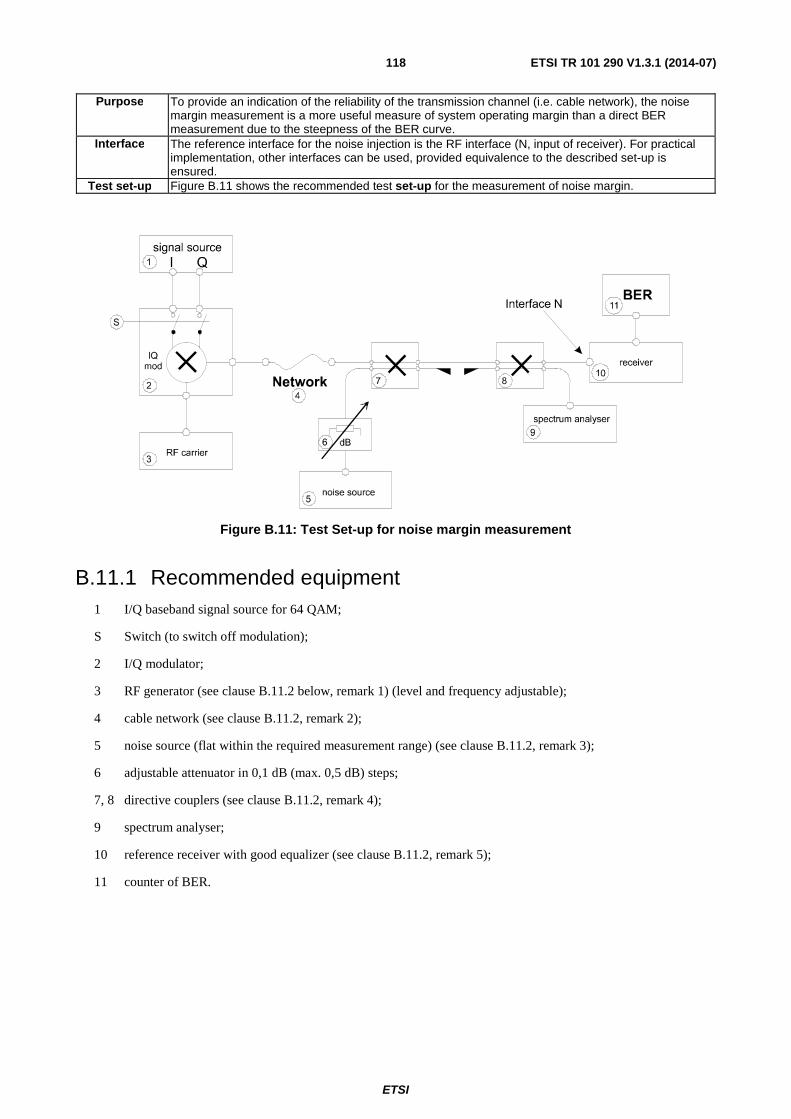
ETSI
ETSI TR 101 290 V1.3.1 (2014-07) 118
Purpose To provide an indication of the reliability of the transmission channel (i.e. cable network), the noise margin measurement is a more useful measure of system operating margin than a direct BER measurement due to the steepness of the BER curve.
Interface The reference interface for the noise injection is the RF interface (N, input of receiver). For practical implementation, other interfaces can be used, provided equivalence to the described set-up is ensured.
Test set-up Figure B.11 shows the recommended test set-up for the measurement of noise margin.
Figure B.11: Test Set-up for noise margin measurement
B.11.1 Recommended equipment 1 I/Q baseband signal source for 64 QAM;
S Switch (to switch off modulation);
2 I/Q modulator;
3 RF generator (see clause B.11.2 below, remark 1) (level and frequency adjustable);
4 cable network (see clause B.11.2, remark 2);
5 noise source (flat within the required measurement range) (see clause B.11.2, remark 3);
6 adjustable attenuator in 0,1 dB (max. 0,5 dB) steps;
7, 8 directive couplers (see clause B.11.2, remark 4);
9 spectrum analyser;
10 reference receiver with good equalizer (see clause B.11.2, remark 5);
11 counter of BER.
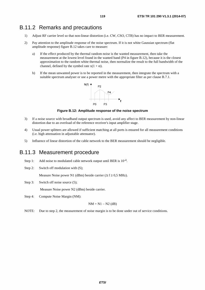
ETSI
ETSI TR 101 290 V1.3.1 (2014-07) 119
B.11.2 Remarks and precautions 1) Adjust RF carrier level so that non-linear distortion (i.e. CW, CSO, CTB) has no impact to BER measurement.
2) Pay attention to the amplitude response of the noise spectrum. If it is not white Gaussian spectrum (flat amplitude response) figure B.12 takes care to measure:
a) If the effect produced by the thermal random noise is the wanted measurement, then take the measurement at the lowest level found in the wanted band (P4 in figure B.12), because it is the closest approximation to the random white thermal noise, then normalize the result to the full bandwidth of the channel, defined by the symbol rate x(1 + α).
b) If the mean unwanted power is to be reported in the measurement, then integrate the spectrum with a suitable spectrum analyser or use a power metre with the appropriate filter as per clause B.7.1.
Figure B.12: Amplitude response of the noise spectrum
3) If a noise source with broadband output spectrum is used, avoid any affect to BER measurement by non-linear distortion due to an overload of the reference receiver's input amplifier stage.
4) Usual power splitters are allowed if sufficient matching at all ports is ensured for all measurement conditions (i.e. high attenuation in adjustable attenuator).
5) Influence of linear distortion of the cable network to the BER measurement should be negligible.
B.11.3 Measurement procedure Step 1: Add noise to modulated cable network output until BER is 10-4.
Step 2: Switch off modulation with (S);
Measure Noise power N1 (dBm) beside carrier (Δ f ≥ 0,5 MHz).
Step 3: Switch off noise source (5);
Measure Noise power N2 (dBm) beside carrier.
Step 4: Compute Noise Margin (NM):
NM = N1 − N2 (dB)
NOTE: Due to step 2, the measurement of noise margin is to be done under out of service conditions.
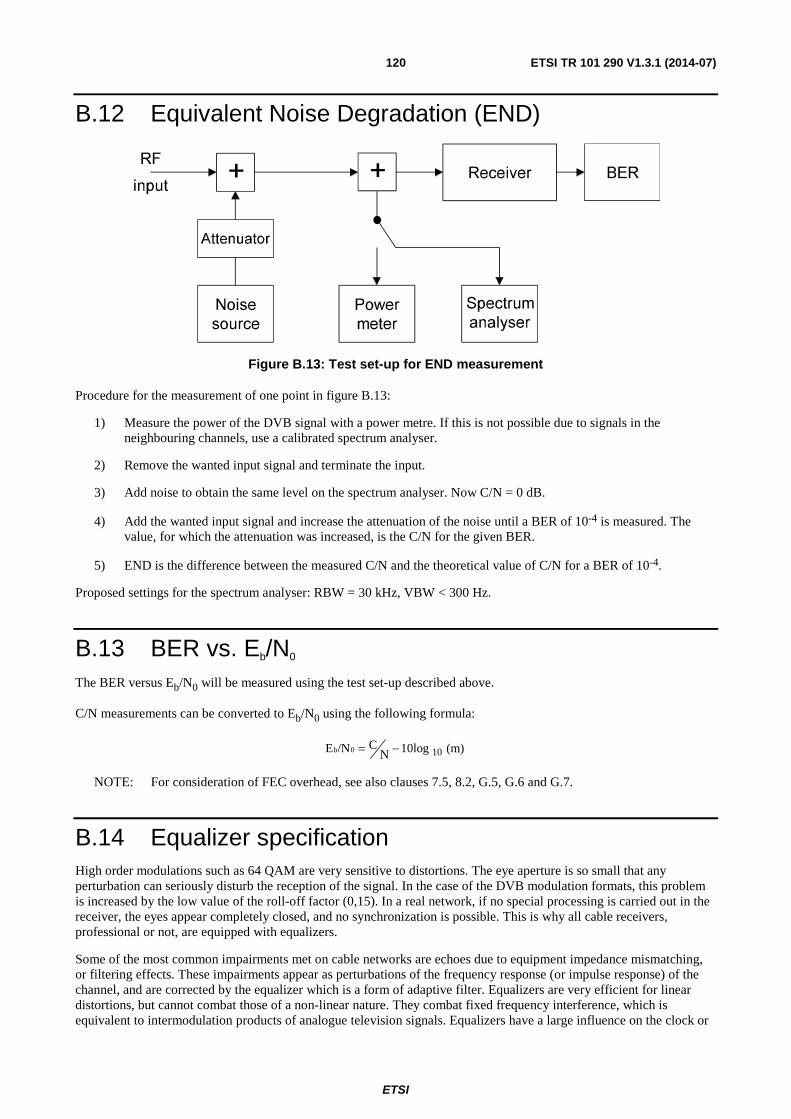
ETSI
ETSI TR 101 290 V1.3.1 (2014-07) 120
B.12 Equivalent Noise Degradation (END)
Figure B.13: Test set-up for END measurement
Procedure for the measurement of one point in figure B.13:
1) Measure the power of the DVB signal with a power metre. If this is not possible due to signals in the neighbouring channels, use a calibrated spectrum analyser.
2) Remove the wanted input signal and terminate the input.
3) Add noise to obtain the same level on the spectrum analyser. Now C/N = 0 dB.
4) Add the wanted input signal and increase the attenuation of the noise until a BER of 10-4 is measured. The value, for which the attenuation was increased, is the C/N for the given BER.
5) END is the difference between the measured C/N and the theoretical value of C/N for a BER of 10-4.
Proposed settings for the spectrum analyser: RBW = 30 kHz, VBW < 300 Hz.
B.13 BER vs. Eb/N0 The BER versus Eb/N0 will be measured using the test set-up described above.
C/N measurements can be converted to Eb/N0 using the following formula:
(m)10logNC /NE 0b 10−=
NOTE: For consideration of FEC overhead, see also clauses 7.5, 8.2, G.5, G.6 and G.7.
B.14 Equalizer specification High order modulations such as 64 QAM are very sensitive to distortions. The eye aperture is so small that any perturbation can seriously disturb the reception of the signal. In the case of the DVB modulation formats, this problem is increased by the low value of the roll-off factor (0,15). In a real network, if no special processing is carried out in the receiver, the eyes appear completely closed, and no synchronization is possible. This is why all cable receivers, professional or not, are equipped with equalizers.
Some of the most common impairments met on cable networks are echoes due to equipment impedance mismatching, or filtering effects. These impairments appear as perturbations of the frequency response (or impulse response) of the channel, and are corrected by the equalizer which is a form of adaptive filter. Equalizers are very efficient for linear distortions, but cannot combat those of a non-linear nature. They combat fixed frequency interference, which is equivalent to intermodulation products of analogue television signals. Equalizers have a large influence on the clock or
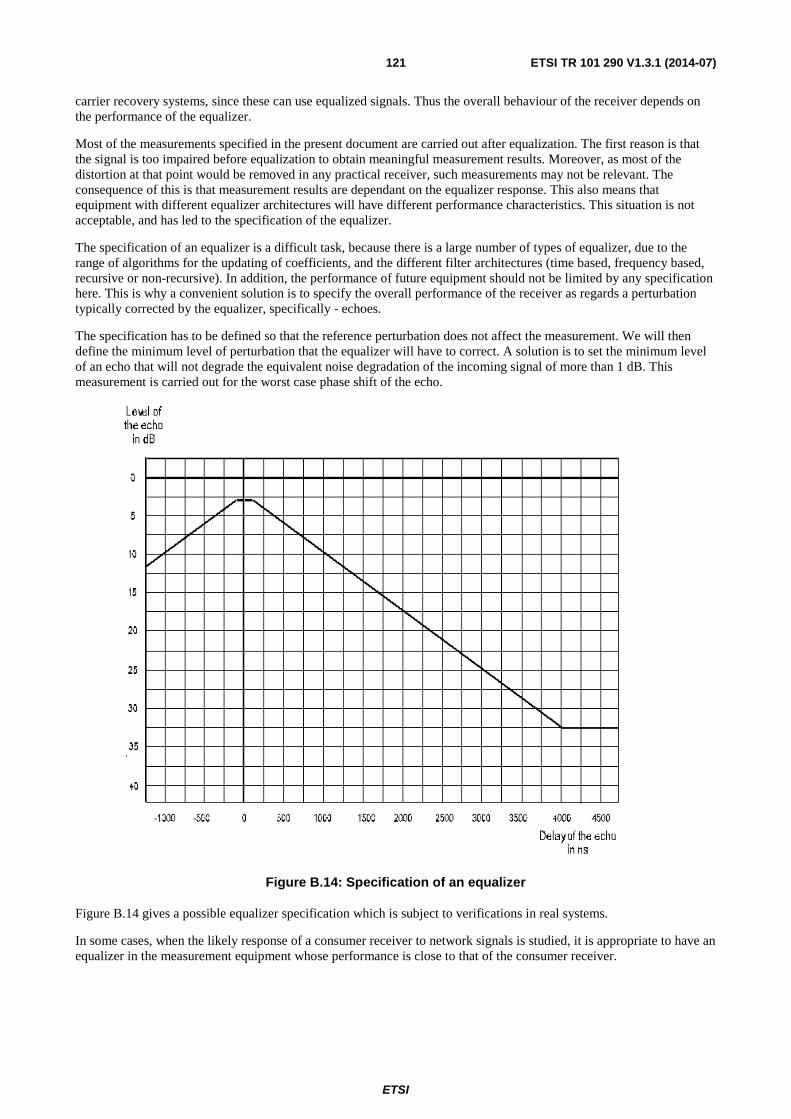
ETSI
ETSI TR 101 290 V1.3.1 (2014-07) 121
carrier recovery systems, since these can use equalized signals. Thus the overall behaviour of the receiver depends on the performance of the equalizer.
Most of the measurements specified in the present document are carried out after equalization. The first reason is that the signal is too impaired before equalization to obtain meaningful measurement results. Moreover, as most of the distortion at that point would be removed in any practical receiver, such measurements may not be relevant. The consequence of this is that measurement results are dependant on the equalizer response. This also means that equipment with different equalizer architectures will have different performance characteristics. This situation is not acceptable, and has led to the specification of the equalizer.
The specification of an equalizer is a difficult task, because there is a large number of types of equalizer, due to the range of algorithms for the updating of coefficients, and the different filter architectures (time based, frequency based, recursive or non-recursive). In addition, the performance of future equipment should not be limited by any specification here. This is why a convenient solution is to specify the overall performance of the receiver as regards a perturbation typically corrected by the equalizer, specifically - echoes.
The specification has to be defined so that the reference perturbation does not affect the measurement. We will then define the minimum level of perturbation that the equalizer will have to correct. A solution is to set the minimum level of an echo that will not degrade the equivalent noise degradation of the incoming signal of more than 1 dB. This measurement is carried out for the worst case phase shift of the echo.
Figure B.14: Specification of an equalizer
Figure B.14 gives a possible equalizer specification which is subject to verifications in real systems.
In some cases, when the likely response of a consumer receiver to network signals is studied, it is appropriate to have an equalizer in the measurement equipment whose performance is close to that of the consumer receiver.

ETSI
ETSI TR 101 290 V1.3.1 (2014-07) 122
B.15 BER before Viterbi decoding This measurement should be based on the I and Q signals at interface T. If an external measurement device is used the signals at interfaces T and V are needed. The set-up is equivalent to figure B.9.
B.16 Receive BER vs. Eb/N0 The measurement is based on transmission of Null packets as defined in clause A.2. At the receiving site noise is added at one of the interfaces N, P or R. The spectrum analyser is used for checking that the normal noise level is well below the added noise. The measurement itself is done either within the receiver or at one of the interfaces T, V or Y depending whether BER before Viterbi, after Viterbi or after RS should be evaluated. In case of interface Y, RS decoding should be deactivated in order to reduce the duration of the measurement.
Figure B.15: Test set-up for BER vs. Eb/N0 measurement
B.17 IF spectrum The output of the modulator should be directly connected to the spectrum analyser. In addition it is also possible to use a (calibrated) splitter.
Figure B.16: Test set-up for IF spectrum measurement
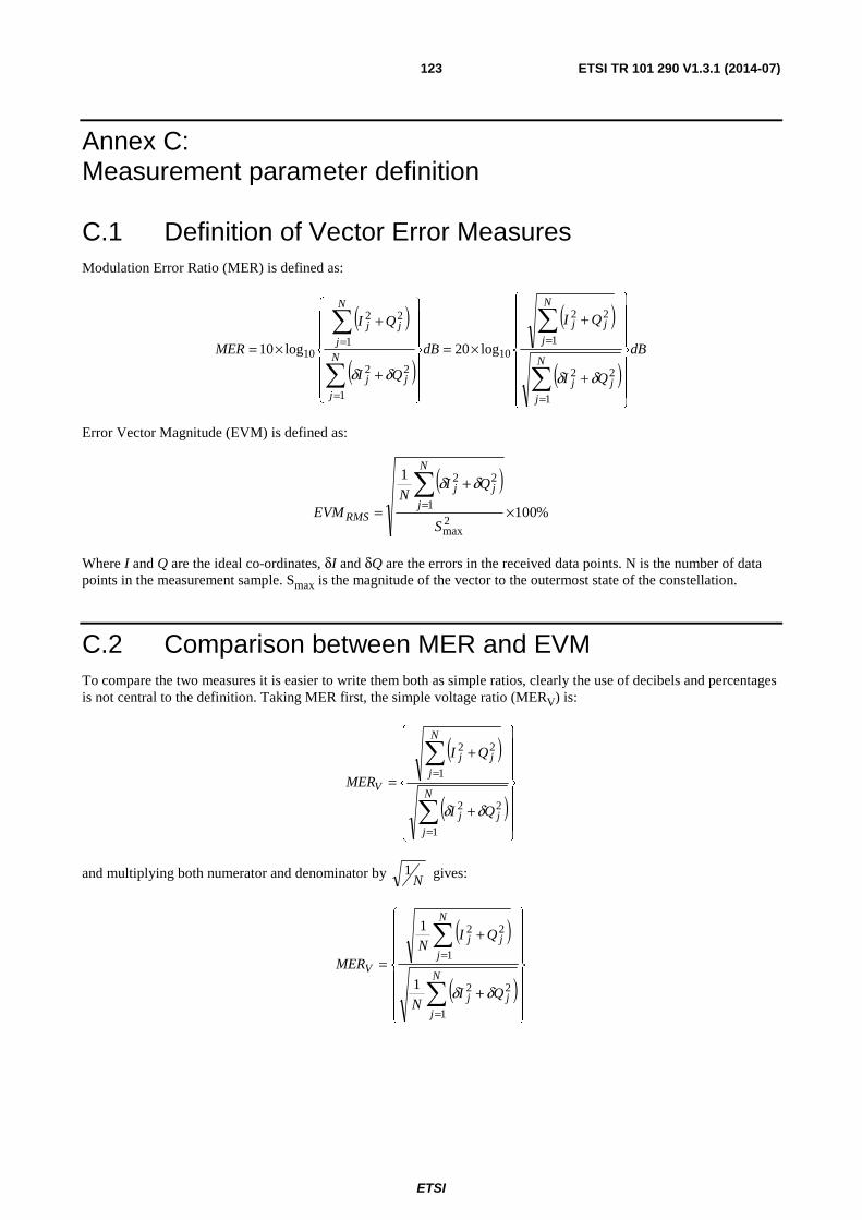
ETSI
ETSI TR 101 290 V1.3.1 (2014-07) 123
Annex C: Measurement parameter definition
C.1 Definition of Vector Error Measures Modulation Error Ratio (MER) is defined as:
( )
( )
( )
( )dB
QI
QI
dB
QI
QI
MERN
j
jj
N
j
jj
N
j
jj
N
j
jj
⎪⎪⎪
⎭
⎪⎪⎪
⎬
⎫
⎪⎪⎪
⎩
⎪⎪⎪
⎨
⎧
+
+
×=
⎪⎪⎪
⎭
⎪⎪⎪
⎬
⎫
⎪⎪⎪
⎩
⎪⎪⎪
⎨
⎧
+
+
×=
∑
∑
∑
∑
=
=
=
=
1
22
1
22
10
1
22
1
22
10 log20log10
δδδδ
Error Vector Magnitude (EVM) is defined as:
( )%100
1
2max
1
22
×
+
=∑
=
S
QIN
EVM
N
j
jj
RMS
δδ
Where I and Q are the ideal co-ordinates, δI and δQ are the errors in the received data points. N is the number of data points in the measurement sample. Smax is the magnitude of the vector to the outermost state of the constellation.
C.2 Comparison between MER and EVM To compare the two measures it is easier to write them both as simple ratios, clearly the use of decibels and percentages is not central to the definition. Taking MER first, the simple voltage ratio (MERV) is:
( )
( )⎪⎪⎪
⎭
⎪⎪⎪
⎬
⎫
⎪⎪⎪
⎩
⎪⎪⎪
⎨
⎧
+
+
=
∑
∑
=
=
N
j
jj
N
j
jj
V
QI
QI
MER
1
22
1
22
δδ
and multiplying both numerator and denominator by N1 gives:
( )
( )⎪⎪⎪
⎭
⎪⎪⎪
⎬
⎫
⎪⎪⎪
⎩
⎪⎪⎪
⎨
⎧
+
+
=
∑
∑
=
=
N
j
jj
N
j
jj
V
QIN
QIN
MER
1
22
1
22
1
1
δδ

ETSI
ETSI TR 101 290 V1.3.1 (2014-07) 124
Now looking at EVM as a simple voltage ratio (EVMV), we can write:
( )max
1
221
S
QIN
EVM
N
j
jj
V
∑=
+
=
δδ
EVM and MER are related such that:
( )max
max
1
22
/1
1
SSVS
QIN
EVMMER rms
N
j
jj
VV ==
+
=×
∑=
or
VMEREVM
VV ×
= 1
If the peak to mean voltage ratio, V, is calculated over a large number of symbols (10 times the number of points in the constellation is adequate if the modulation is random) and each symbol has the same probability of occurrence then it is a constant for a given transmission system. The value tends to a limit which can be calculated by considering the peak to mean of all the constellation points. Table A.2 lists the peak- to-mean voltage ratios for the DVB constellation sizes.
Table C.1: Peak-to-mean ratios for the DVB constellation sizes
QAM format Peak-to-mean voltage ratio (V)
16 1 341 32 1 303 64 1 527
C.3 Conclusions regarding MER and EVM MER and EVM measure essentially the same quantity and easy conversion is possible between the two measures if the constellation is known. When expressed as simple voltage ratios MERV is equal to the reciprocal of the product of
EVMV and the peak-to-mean voltage ratio for the constellation.
MER is the preferred measurement for the following reasons:
- The sensitivity of the measurement, the typical magnitude of measured values, and the units of measurement combine to give MER an immediate familiarity for those who have previous experience of C/N or SNR measurement.
- MER can be regarded as a form of Signal-to-Noise ratio measurement that will give an accurate indication of a receiver's ability to demodulate the signal, because it includes, not just Gaussian noise, but all other uncorrectable impairments of the received constellation as well.
- If the only significant impairment present in the signal is Gaussian noise then MER and SNR are equivalent.

ETSI
ETSI TR 101 290 V1.3.1 (2014-07) 125
Annex D: Exact values of BER vs. Eb/N0 for DVB-C systems Exact values of BER vs. Eb/N0 for DVB-C systems (see figure 7.2).
Table D.1: Exact values of BER vs. Eb/N0 for DVB-C systems
Eb/N0 Pb
10 0,025 48 10,5 0,020 72 11 0,016 46 11,5 0,012 74 12 0,009 582 12,5 0,006 981 13 0,004 909 13,5 0,003 319 14 0,002 147 14,5 0,001 323 15 0,000 771 6 15,5 0,000 423 5 16 0,000 217 1 16,5 0,000 103 1 17 4,499e-005 17,5 1,783e-005 18 6,351e-006 18,5 2,006e-006 19 5,537e-007 19,5 1,314e-007 20 2,634e-008 20,5 4,365e-009 21 5,846e-010 21,5 6,166e-011 22 4,974e-012
This assumes that the relationship between BER and Symbol Error Rate (SER) is given by the formula:
SERm
BER ×= 1
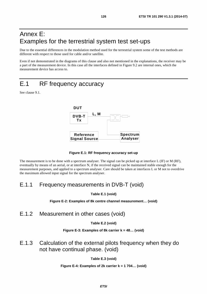
ETSI
ETSI TR 101 290 V1.3.1 (2014-07) 126
Annex E: Examples for the terrestrial system test set-ups Due to the essential differences in the modulation method used for the terrestrial system some of the test methods are different with respect to those used for cable and/or satellite.
Even if not demonstrated in the diagrams of this clause and also not mentioned in the explanations, the receiver may be a part of the measurement device. In this case all the interfaces defined in Figure 9.2 are internal ones, which the measurement device has access to.
E.1 RF frequency accuracy See clause 9.1.
DVB-T Tx
Reference Signal Source
Spectrum Analyser
DUT
L, M
Figure E.1: RF frequency accuracy set-up
The measurement is to be done with a spectrum analyser. The signal can be picked up at interface L (IF) or M (RF), eventually by means of an aerial, or at interface N, if the received signal can be maintained stable enough for the measurement purposes, and applied to a spectrum analyser. Care should be taken at interfaces L or M not to overdrive the maximum allowed input signal for the spectrum analyser.
E.1.1 Frequency measurements in DVB-T (void)
Table E.1 (void)
Figure E-2: Examples of 8k centre channel measurement… (void)
E.1.2 Measurement in other cases (void)
Table E.2 (void)
Figure E-3: Examples of 8k carrier k = 48… (void)
E.1.3 Calculation of the external pilots frequency when they do not have continual phase. (void)
Table E.3 (void)
Figure E-4: Examples of 2k carrier k = 1 704… (void)

ETSI
ETSI TR 101 290 V1.3.1 (2014-07) 127
Figure E-5: Examples of 8k carrier k = 6 816… (void)
Figure E-6: Examples of 2k carrier k = 0… (void)
Figure E-7: Examples of 2k carrier k = 0… (void)
Table E.4 (void)
E.1.4 Measuring the symbol length and verifying the Guard Interval (void)
Table E.5 (void)
Figure E-8: Examples of 8k carrier k = 6 813… (void)
Table E.6 (void)
Table E.7 (void)
Table E.8 (void)
Figure E-9: Examples of 2k carrier k = 1 701… (void)
E.1.5 Measuring the occupied bandwidth, and calculation of the frequency spacing and sampling frequency
The occupied bandwidth depends directly from the frequency spacing and this from the sampling frequency.
If the frequency of the external pilots is known, see above on how to measure them, then the related values may be calculated as per table below. Denoting the outermost pilot frequencies as FL and FH appropriately the occupied
bandwidth is OB = FH _ FL. The number of carriers K, and for 2k mode K-1 = 1 704 while for 8k mode K-1 = 6 816.
Table E.9
Calculated value Nominal value (8 MHz Channels) 8k mode 2k mode 8k mode 2k mode
Occupied bandwidth FH - FL 7,60714285714285714285714285714286… MHz
Frequency Spacing (FH - FL)/6 816 (FH - FL)/1 704 1 116,0714285…Hz 4 464,2857142…Hz
Useful duration 6 816/(FH - FL) 1 704/(FH - FL) 896 μs 224 μs
Centre channel 1st IF (FH - FL) × 4 096/(K-1) (FH - FL) × 1 024/(K-1) 4,57142857142857142857142857142857…MHz
Sampling Frequency (FH - FL) × 16 384/(K-1) (FH - FL) × 4 096/(K-1) 18,2857142857142857142857142857143…MHz
NOTE: The long periodic decimals have been calculated using the Calculator facility from Windows, and have been left here as resulted from copying through the clipboard, as a matter of curiosity only.
Values in italics are approximate values.
Table E.10
Nominal value (7 MHz Channels) Nominal value (6 MHz Channels) 8k mode 2k mode 8k mode 2k mode
Occupied bandwidth 6.656250 MHz 5,70535714285714285714285714285842… MHz
Frequency Spacing 976,5625 Hz 3 906,25 Hz 837,053571428571…Hz 3 348,2142857142…Hz
Useful duration 1 024 μs 256 μs 1 194,666666… μs 298,666666… μs
Centre channel 1st IF 4 MHz 3,42857142857142857142857142857334…MHz
Sampling Frequency 16 MHz 13,7142857142857142857142857142934…MHz
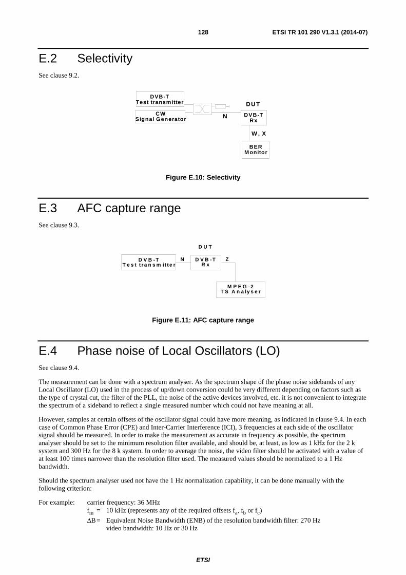
ETSI
ETSI TR 101 290 V1.3.1 (2014-07) 128
E.2 Selectivity See clause 9.2.
DVB-T Test transmitter
CW Signal Generator
DVB-T Rx
BER Monitor
N
W , X
DUT
Figure E.10: Selectivity
E.3 AFC capture range See clause 9.3.
D V B -T R x
M P E G -2 T S A n a ly s e r
D U T
N Z D V B -T T e s t t r a n s m it te r
Figure E.11: AFC capture range
E.4 Phase noise of Local Oscillators (LO) See clause 9.4.
The measurement can be done with a spectrum analyser. As the spectrum shape of the phase noise sidebands of any Local Oscillator (LO) used in the process of up/down conversion could be very different depending on factors such as the type of crystal cut, the filter of the PLL, the noise of the active devices involved, etc. it is not convenient to integrate the spectrum of a sideband to reflect a single measured number which could not have meaning at all.
However, samples at certain offsets of the oscillator signal could have more meaning, as indicated in clause 9.4. In each case of Common Phase Error (CPE) and Inter-Carrier Interference (ICI), 3 frequencies at each side of the oscillator signal should be measured. In order to make the measurement as accurate in frequency as possible, the spectrum analyser should be set to the minimum resolution filter available, and should be, at least, as low as 1 kHz for the 2 k system and 300 Hz for the 8 k system. In order to average the noise, the video filter should be activated with a value of at least 100 times narrower than the resolution filter used. The measured values should be normalized to a 1 Hz bandwidth.
Should the spectrum analyser used not have the 1 Hz normalization capability, it can be done manually with the following criterion:
For example: carrier frequency: 36 MHz fm = 10 kHz (represents any of the required offsets fa, fb or fc)
ΔB = Equivalent Noise Bandwidth (ENB) of the resolution bandwidth filter: 270 Hz video bandwidth: 10 Hz or 30 Hz
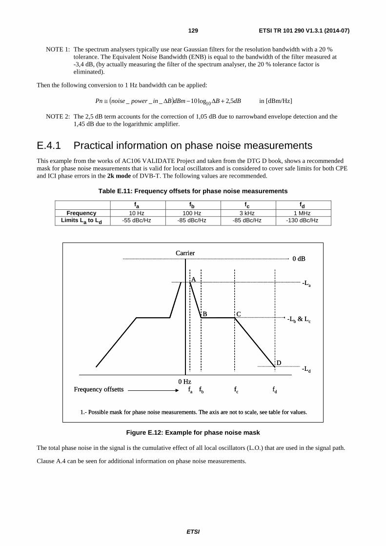
ETSI
ETSI TR 101 290 V1.3.1 (2014-07) 129
NOTE 1: The spectrum analysers typically use near Gaussian filters for the resolution bandwidth with a 20 % tolerance. The Equivalent Noise Bandwidth (ENB) is equal to the bandwidth of the filter measured at -3,4 dB, (by actually measuring the filter of the spectrum analyser, the 20 % tolerance factor is eliminated).
Then the following conversion to 1 Hz bandwidth can be applied:
( ) dBBdBmBinpowernoisePn 5,2log10___ 10 +Δ−Δ≅ in [dBm/Hz]
NOTE 2: The 2,5 dB term accounts for the correction of 1,05 dB due to narrowband envelope detection and the 1,45 dB due to the logarithmic amplifier.
E.4.1 Practical information on phase noise measurements This example from the works of AC106 VALIDATE Project and taken from the DTG D book, shows a recommended mask for phase noise measurements that is valid for local oscillators and is considered to cover safe limits for both CPE and ICI phase errors in the 2k mode of DVB-T. The following values are recommended.
Table E.11: Frequency offsets for phase noise measurements
fa fb fc fd
Frequency 10 Hz 100 Hz 3 kHz 1 MHz Limits La to Ld -55 dBc/Hz -85 dBc/Hz -85 dBc/Hz -130 dBc/Hz
A
B C
fa fb fc
-La
-Lb & Lc
-Ld
0 dB
0 HzFrequency offsetts
Carrier
1.- Possible mask for phase noise measurements. The axis are not to scale, see table for values.
D
fd
A
B C
fa fb fc
-La
-Lb & Lc
-Ld
0 dB
0 HzFrequency offsetts
Carrier
1.- Possible mask for phase noise measurements. The axis are not to scale, see table for values.
D
fd
Figure E.12: Example for phase noise mask
The total phase noise in the signal is the cumulative effect of all local oscillators (L.O.) that are used in the signal path.
Clause A.4 can be seen for additional information on phase noise measurements.
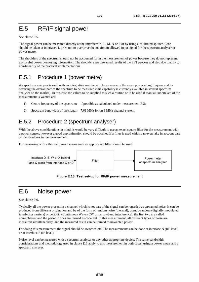
ETSI
ETSI TR 101 290 V1.3.1 (2014-07) 130
E.5 RF/IF signal power See clause 9.5.
The signal power can be measured directly at the interfaces K, L, M, N or P or by using a calibrated splitter. Care should be taken at interfaces L or M not to overdrive the maximum allowed input signal for the spectrum analyser or power metre.
The shoulders of the spectrum should not be accounted for in the measurement of power because they do not represent any useful power conveying information. The shoulders are unwanted results of the FFT process and also due mainly to non-linearity of the practical implementations.
E.5.1 Procedure 1 (power metre) An spectrum analyser is used with an integrating routine which can measure the mean power along frequency slots covering the overall part of the spectrum to be measured (this capability is currently available in several spectrum analyser on the market). In this case the values to be supplied to such a routine or to be used if manual undertaken of the measurement is wanted are:
1) Centre frequency of the spectrum: if possible as calculated under measurement E.2;
2) Spectrum bandwidth of the signal: 7,61 MHz for an 8 MHz channel system.
E.5.2 Procedure 2 (spectrum analyser) With the above considerations in mind, it would be very difficult to use an exact square filter for the measurement with a power sensor, however a good approximation should be obtained if a filter is used which can even take in account part of the shoulders in the measurement.
For measuring with a thermal power sensor such an appropriate filter should be used.
Figure E.13: Test set-up for RF/IF power measurement
E.6 Noise power See clause 9.6.
Typically all the power present in a channel which is not part of the signal can be regarded as unwanted noise. It can be produced from different origination and be of the form of random noise (thermal), pseudo-random (digitally modulated interfering carriers) or periodic (Continuous Waves CW or narrowband interference), the first two are called non-coherent and the periodic ones are termed as coherent. In this measurement, all different types of noise are measured simultaneously, and the measured result can be termed as unwanted power.
For doing this measurement the signal should be switched off. The measurements can be done at interface N (RF level) or at interface P (IF level).
Noise level can be measured with a spectrum analyser or any other appropriate device. The same bandwidth considerations and methodology used in clause E.6 apply to this measurement in both cases, using a power metre and a spectrum analyser.
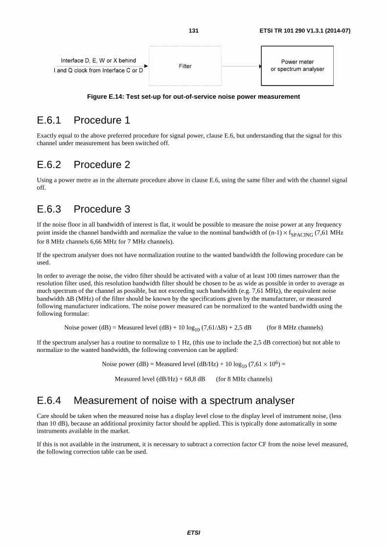
ETSI
ETSI TR 101 290 V1.3.1 (2014-07) 131
Figure E.14: Test set-up for out-of-service noise power measurement
E.6.1 Procedure 1 Exactly equal to the above preferred procedure for signal power, clause E.6, but understanding that the signal for this channel under measurement has been switched off.
E.6.2 Procedure 2 Using a power metre as in the alternate procedure above in clause E.6, using the same filter and with the channel signal off.
E.6.3 Procedure 3 If the noise floor in all bandwidth of interest is flat, it would be possible to measure the noise power at any frequency point inside the channel bandwidth and normalize the value to the nominal bandwidth of (n-1) × fSPACING (7,61 MHz
for 8 MHz channels 6,66 MHz for 7 MHz channels).
If the spectrum analyser does not have normalization routine to the wanted bandwidth the following procedure can be used.
In order to average the noise, the video filter should be activated with a value of at least 100 times narrower than the resolution filter used, this resolution bandwidth filter should be chosen to be as wide as possible in order to average as much spectrum of the channel as possible, but not exceeding such bandwidth (e.g. 7,61 MHz), the equivalent noise bandwidth ΔB (MHz) of the filter should be known by the specifications given by the manufacturer, or measured following manufacturer indications. The noise power measured can be normalized to the wanted bandwidth using the following formulae:
Noise power (dB) = Measured level (dB) + 10 log10 (7,61/ΔB) + 2,5 dB (for 8 MHz channels)
If the spectrum analyser has a routine to normalize to 1 Hz, (this use to include the 2,5 dB correction) but not able to normalize to the wanted bandwidth, the following conversion can be applied:
Noise power (dB) = Measured level (dB/Hz) + 10 log10 (7,61 × 10⁶) =
Measured level (dB/Hz) + 68,8 dB (for 8 MHz channels)
E.6.4 Measurement of noise with a spectrum analyser Care should be taken when the measured noise has a display level close to the display level of instrument noise, (less than 10 dB), because an additional proximity factor should be applied. This is typically done automatically in some instruments available in the market.
If this is not available in the instrument, it is necessary to subtract a correction factor CF from the noise level measured, the following correction table can be used.
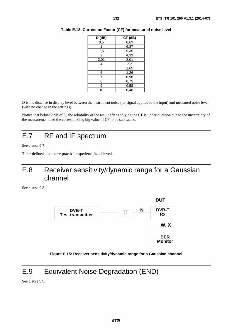
ETSI
ETSI TR 101 290 V1.3.1 (2014-07) 132
Table E.12: Correction Factor (CF) for measured noise level
D (dB) CF (dB) 0,5 8,63 1 6,87
1,5 5,35 2 4,33
3,01 3,01 4 2,2 5 1,65 6 1,26 7 0,98 8 0,75 9 0,58
10 0,46
D is the distance in display level between the instrument noise (no signal applied to the input) and measured noise level (with no change in the settings).
Notice that below 2 dB of D, the reliability of the result after applying the CF is under question due to the uncertainty of the measurement and the corresponding big value of CF to be subtracted.
E.7 RF and IF spectrum See clause 9.7.
To be defined after some practical experience is achieved.
E.8 Receiver sensitivity/dynamic range for a Gaussian channel
See clause 9.8.
N
W, X
DUT
DVB-TTest transmitter
DVB-TRx
BERMonitor
Figure E.15: Receiver sensitivity/dynamic range for a Gaussian channel
E.9 Equivalent Noise Degradation (END) See clause 9.9.

ETSI
ETSI TR 101 290 V1.3.1 (2014-07) 133
N , P , S
W , X
D VB -T Tx
D V B -T R x
N oise G en erato r
B E R M o nito r
Figure E.16: Equivalent Noise Degradation (END)
All measurements of performance parameters are carried out by using a dummy load which provides a return loss for the wanted channel which is low enough not to influence the measurement.
E.9.1 Description of the measurement method for END To improve the accuracy of the measurement, two independent noise sources are used. By this, the influence of the tolerance of the first attenuator is eliminated which could well be in the same magnitude as the wanted measurement result.
The following steps should be carried out to arrive at an accurate ENF value:
1) Connect the real DVB-T transmitter to the DVB-T receiver and add Gaussian noise, Ncal, to the point where
the BER reaches a pre-determined value (e.g. 2 x 10⁻⁴ after Viterbi decoding). Ncal does not have to be
measured. No channel noise, Nch, should be added. The C/N at the input to the receiver (Interface C) is
therefore C/(Ntx + Ncal).
2) Replace the real DVB-T transmitter by the ideal one (disconnect Ntx in figure E.17). The C/N at Interface C is
now somewhat higher (C/Ncal), since Ntx is no longer present. The BER is therefore now lower than the
predetermined value.
3) Add Gaussian channel noise, Nch, to the point where the BER has reached its predetermined value again. The
C/N at interface C is now C/(Nch + Ncal).
4) Measure the value of C/Nch at Interface B.
+ + + Ideal DVB-T Tx
NcalNchNtx
Unknown DVB-T Rx
Real DVB-T Tx
FixedBER=2 x 10⁻⁴
after Viterbi orRS decoding
C
Interface A
Interface B
Interface C
Figure E.17: ENF measurement scheme

ETSI
ETSI TR 101 290 V1.3.1 (2014-07) 134
Since both C/(Ntx + Ncal) and C/(Nch + Ncal) lead to the same BER, Nch can be identified with Ntx and be regarded as
an estimate of Ntx.
The ENF is defined to be 10 10log(Ntx/C). The estimated ENF value is similarly 10 10log(Nch/C)
As long as all distortions of a DVB-T transmitter can be well approximated by the Gaussian noise, Ntx, the ENF
measurement, as described above, should be completely independent of both the DVB-T mode and the receiver characteristics. For highest measurement accuracy the measurement should however preferably be done using the (non-hierarchical) mode requiring the highest C/N, i.e. 64-QAM R=7/8.
In practice, there might however be selective effects such as amplitude ripple and spurious signals within the useful bandwidth. In these cases the ENF will in principle be better (= a more negative value) when stronger code rates are used (such as R = 1/2 or 2/3) than when weaker codes are used (such as R = 5/6 or 7/8). Whether this difference is measureable or not remains to be seen. It is therefore recommendable to measure the ENF also for the other code rates. If there is negligible difference between the ENF figures for the different code rates, this will imply that there are few selective effects and/or that these effects can be well approximated by Gaussian noise. If however there is a significant difference in ENF figures this implies that the ENF (and hence END) is code rate dependent. In such a case the ENF value to be used (either by itself or for the calculated END) should preferably be the one measured with the same code rate as the DVB-T transmitter will be used with by the network operator.
E.9.2 Conversion method between ENF and END Let (C/N)min, theory be the minimum C/N requirement for a DVB-T mode given by EN 300 744 [i.9].
Assume an implementation loss of 3,0 dB for all modes. Let X = (C/N)min, real be the corresponding minimum required C/N for a DVB-T mode.
X = (C/N)min, real = (C/N)min, theory + 3,0 dB
END can be calculated from ENF by the formula:
END = -10 10log(10 -X/10 -10 ENF/10) - X
Example:
X = 19,5 dB (64QAM, R= 2/3) ENF = -30,0 dB
END = -10 10log(10 -19,5/10 -10 -30,0/10) - 19,5 dB = 0,41 dB
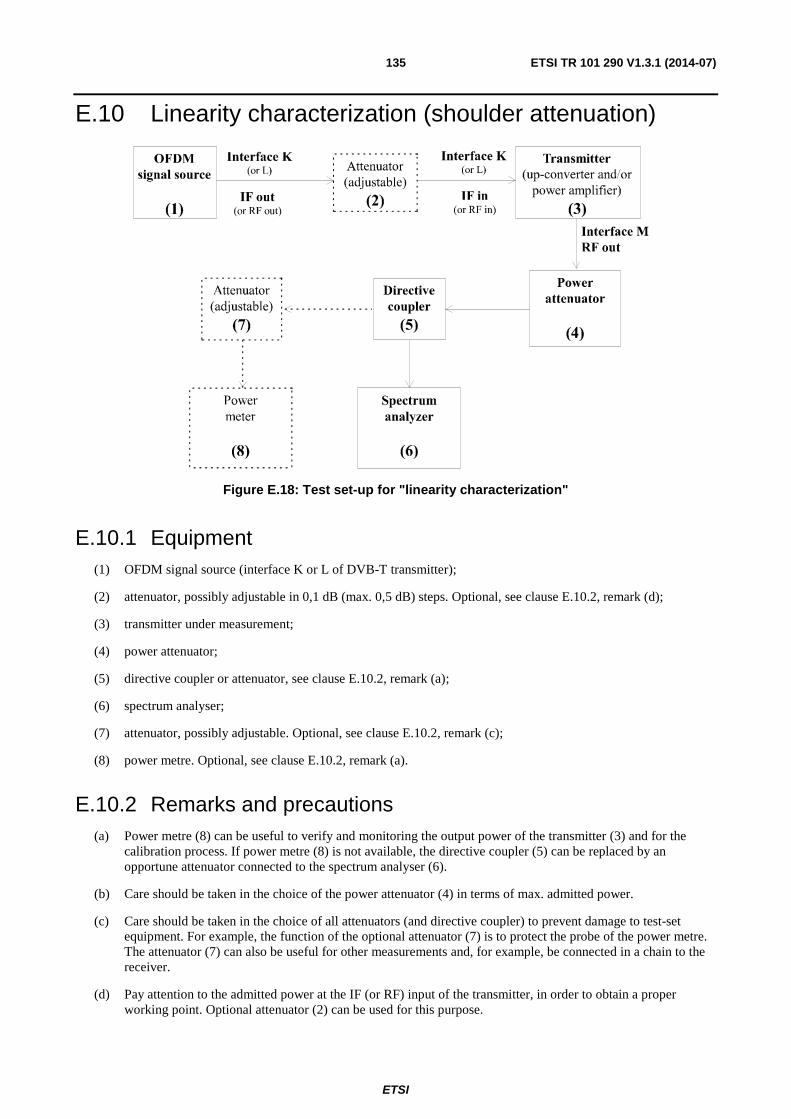
ETSI
ETSI TR 101 290 V1.3.1 (2014-07) 135
E.10 Linearity characterization (shoulder attenuation)
Figure E.18: Test set-up for "linearity characterization"
E.10.1 Equipment (1) OFDM signal source (interface K or L of DVB-T transmitter);
(2) attenuator, possibly adjustable in 0,1 dB (max. 0,5 dB) steps. Optional, see clause E.10.2, remark (d);
(3) transmitter under measurement;
(4) power attenuator;
(5) directive coupler or attenuator, see clause E.10.2, remark (a);
(6) spectrum analyser;
(7) attenuator, possibly adjustable. Optional, see clause E.10.2, remark (c);
(8) power metre. Optional, see clause E.10.2, remark (a).
E.10.2 Remarks and precautions (a) Power metre (8) can be useful to verify and monitoring the output power of the transmitter (3) and for the
calibration process. If power metre (8) is not available, the directive coupler (5) can be replaced by an opportune attenuator connected to the spectrum analyser (6).
(b) Care should be taken in the choice of the power attenuator (4) in terms of max. admitted power.
(c) Care should be taken in the choice of all attenuators (and directive coupler) to prevent damage to test-set equipment. For example, the function of the optional attenuator (7) is to protect the probe of the power metre. The attenuator (7) can also be useful for other measurements and, for example, be connected in a chain to the receiver.
(d) Pay attention to the admitted power at the IF (or RF) input of the transmitter, in order to obtain a proper working point. Optional attenuator (2) can be used for this purpose.
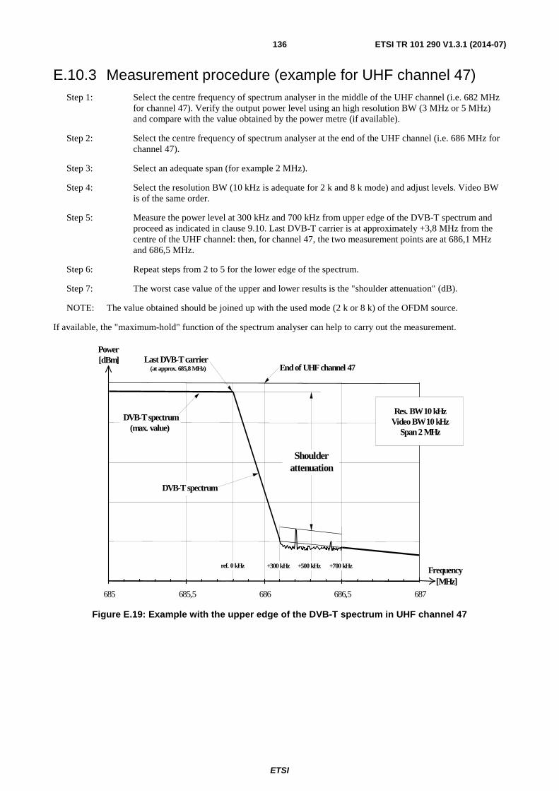
ETSI
ETSI TR 101 290 V1.3.1 (2014-07) 136
E.10.3 Measurement procedure (example for UHF channel 47) Step 1: Select the centre frequency of spectrum analyser in the middle of the UHF channel (i.e. 682 MHz
for channel 47). Verify the output power level using an high resolution BW (3 MHz or 5 MHz) and compare with the value obtained by the power metre (if available).
Step 2: Select the centre frequency of spectrum analyser at the end of the UHF channel (i.e. 686 MHz for channel 47).
Step 3: Select an adequate span (for example 2 MHz).
Step 4: Select the resolution BW (10 kHz is adequate for 2 k and 8 k mode) and adjust levels. Video BW is of the same order.
Step 5: Measure the power level at 300 kHz and 700 kHz from upper edge of the DVB-T spectrum and proceed as indicated in clause 9.10. Last DVB-T carrier is at approximately +3,8 MHz from the centre of the UHF channel: then, for channel 47, the two measurement points are at 686,1 MHz and 686,5 MHz.
Step 6: Repeat steps from 2 to 5 for the lower edge of the spectrum.
Step 7: The worst case value of the upper and lower results is the "shoulder attenuation" (dB).
NOTE: The value obtained should be joined up with the used mode (2 k or 8 k) of the OFDM source.
If available, the "maximum-hold" function of the spectrum analyser can help to carry out the measurement.
685 685,5 686 686,5 687
Power [dBm]
Res. BW 10 kHz Video BW 10 kHz
Span 2 MHz
Shoulder attenuation
+700 kHz +500 kHz +300 kHz
End of UHF channel 47 Last DVB-T carrier
(at approx. 685,8 MHz)
DVB-T spectrum (max. value)
ref. 0 kHz
DVB-T spectrum
Frequency [MHz]
Figure E.19: Example with the upper edge of the DVB-T spectrum in UHF channel 47
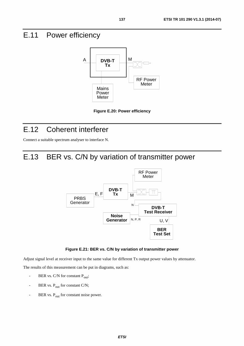
ETSI
ETSI TR 101 290 V1.3.1 (2014-07) 137
E.11 Power efficiency
DVB-TTx
MainsPowerMeter
RF PowerMeter
A M
Figure E.20: Power efficiency
E.12 Coherent interferer Connect a suitable spectrum analyser to interface N.
E.13 BER vs. C/N by variation of transmitter power
DVB-TTx
NoiseGenerator
RF PowerMeter
MPRBS
Generator
E, F
BERTest Set
DVB-TTest Receiver
U, VN, P, R
N
Figure E.21: BER vs. C/N by variation of transmitter power
Adjust signal level at receiver input to the same value for different Tx output power values by attenuator.
The results of this measurement can be put in diagrams, such as:
- BER vs. C/N for constant Pout;
- BER vs. Pout for constant C/N;
- BER vs. Pout for constant noise power.
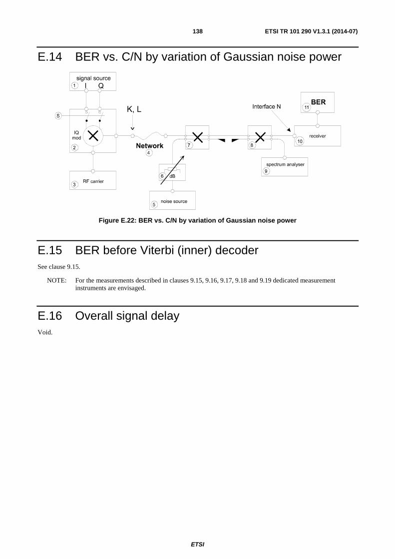
ETSI
ETSI TR 101 290 V1.3.1 (2014-07) 138
E.14 BER vs. C/N by variation of Gaussian noise power
Figure E.22: BER vs. C/N by variation of Gaussian noise power
E.15 BER before Viterbi (inner) decoder See clause 9.15.
NOTE: For the measurements described in clauses 9.15, 9.16, 9.17, 9.18 and 9.19 dedicated measurement instruments are envisaged.
E.16 Overall signal delay Void.
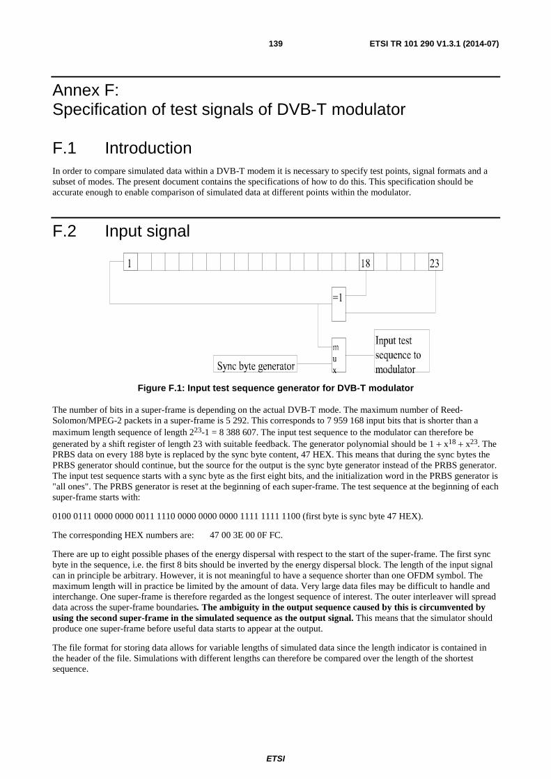
ETSI
ETSI TR 101 290 V1.3.1 (2014-07) 139
Annex F: Specification of test signals of DVB-T modulator
F.1 Introduction In order to compare simulated data within a DVB-T modem it is necessary to specify test points, signal formats and a subset of modes. The present document contains the specifications of how to do this. This specification should be accurate enough to enable comparison of simulated data at different points within the modulator.
F.2 Input signal
Figure F.1: Input test sequence generator for DVB-T modulator
The number of bits in a super-frame is depending on the actual DVB-T mode. The maximum number of Reed-Solomon/MPEG-2 packets in a super-frame is 5 292. This corresponds to 7 959 168 input bits that is shorter than a maximum length sequence of length 223-1 = 8 388 607. The input test sequence to the modulator can therefore be generated by a shift register of length 23 with suitable feedback. The generator polynomial should be 1 + x18 + x23. The PRBS data on every 188 byte is replaced by the sync byte content, 47 HEX. This means that during the sync bytes the PRBS generator should continue, but the source for the output is the sync byte generator instead of the PRBS generator. The input test sequence starts with a sync byte as the first eight bits, and the initialization word in the PRBS generator is "all ones". The PRBS generator is reset at the beginning of each super-frame. The test sequence at the beginning of each super-frame starts with:
0100 0111 0000 0000 0011 1110 0000 0000 0000 1111 1111 1100 (first byte is sync byte 47 HEX).
The corresponding HEX numbers are: 47 00 3E 00 0F FC.
There are up to eight possible phases of the energy dispersal with respect to the start of the super-frame. The first sync byte in the sequence, i.e. the first 8 bits should be inverted by the energy dispersal block. The length of the input signal can in principle be arbitrary. However, it is not meaningful to have a sequence shorter than one OFDM symbol. The maximum length will in practice be limited by the amount of data. Very large data files may be difficult to handle and interchange. One super-frame is therefore regarded as the longest sequence of interest. The outer interleaver will spread data across the super-frame boundaries. The ambiguity in the output sequence caused by this is circumvented by using the second super-frame in the simulated sequence as the output signal. This means that the simulator should produce one super-frame before useful data starts to appear at the output.
The file format for storing data allows for variable lengths of simulated data since the length indicator is contained in the header of the file. Simulations with different lengths can therefore be compared over the length of the shortest sequence.

ETSI
ETSI TR 101 290 V1.3.1 (2014-07) 140
F.3 Test modes The file header in the test file contains information about the specific DVB-T mode used for the simulation. By reading this information a complete description of the set-up is obtained. In order to ease comparison of data and to reduce the amount of simulations necessary a set of "preferred modes" are defined. The preferred test mode for non-hierarchical transmission is:
Inner code rate: 2/3;
Modulation method: 64 QAM;
FFT size: 8 k;
Guard interval: 1/32.
For hierarchical transmission the preferred mode is:
Inner code rate HP: 2/3;
Inner code rate LP: 3/4;
Modulation method: QPSK in 64 QAM, α = 2;
FFT size: 8 k;
Guard interval: 1/32.
F.4 Test points The simulated data can be probed at different points within the modulator. Eight test points are defined, which are related to the interfaces described in figure 9.1:
1) at input (A);
2) after mux adaptation, energy dispersal (B);
3) after outer encoder (C);
4) after outer interleaver (D);
5) after inner encoder (E);
6) after inner interleaver (F);
7) after frame adaptation (H);
8) after guard interval insertion (J).
F.5 File format for interchange of simulated data The file header as well as simulated data from the modem are stored as ASCII characters on files with carriage return and line feed at the end of each line. In order to interchange data it is important that the same file format be used by everyone. A file containing such data should have a header which has the following information:
- text string with a maximum of 80 characters (affiliation, time, place etc.);
- "printf" string used to store the data in the data section of the file;
- test point description;
- length of data buffer;
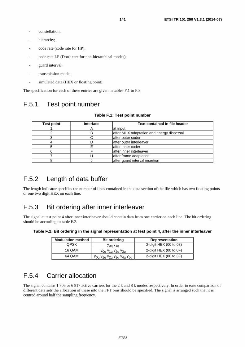
ETSI
ETSI TR 101 290 V1.3.1 (2014-07) 141
- constellation;
- hierarchy;
- code rate (code rate for HP);
- code rate LP (Don't care for non-hierarchical modes);
- guard interval;
- transmission mode;
- simulated data (HEX or floating point).
The specification for each of these entries are given in tables F.1 to F.8.
F.5.1 Test point number
Table F.1: Test point number
Test point Interface Text contained in file header 1 A at input 2 B after MUX adaptation and energy dispersal 3 C after outer coder 4 D after outer interleaver 5 E after inner coder 6 F after inner interleaver 7 H after frame adaptation 8 J after guard interval insertion
F.5.2 Length of data buffer The length indicator specifies the number of lines contained in the data section of the file which has two floating points or one two digit HEX on each line.
F.5.3 Bit ordering after inner interleaver The signal at test point 4 after inner interleaver should contain data from one carrier on each line. The bit ordering should be according to table F.2.
Table F.2: Bit ordering in the signal representation at test point 4, after the inner interleaver
Modulation method Bit ordering Representation QPSK y0q y1q 2-digit HEX (00 to 03)
16 QAM y0q y1q y2q y3q 2-digit HEX (00 to 0F)
64 QAM y0q y1q y2q y3q y4q y5q 2-digit HEX (00 to 3F)
F.5.4 Carrier allocation The signal contains 1 705 or 6 817 active carriers for the 2 k and 8 k modes respectively. In order to ease comparison of different data sets the allocation of these into the FFT bins should be specified. The signal is arranged such that it is centred around half the sampling frequency.
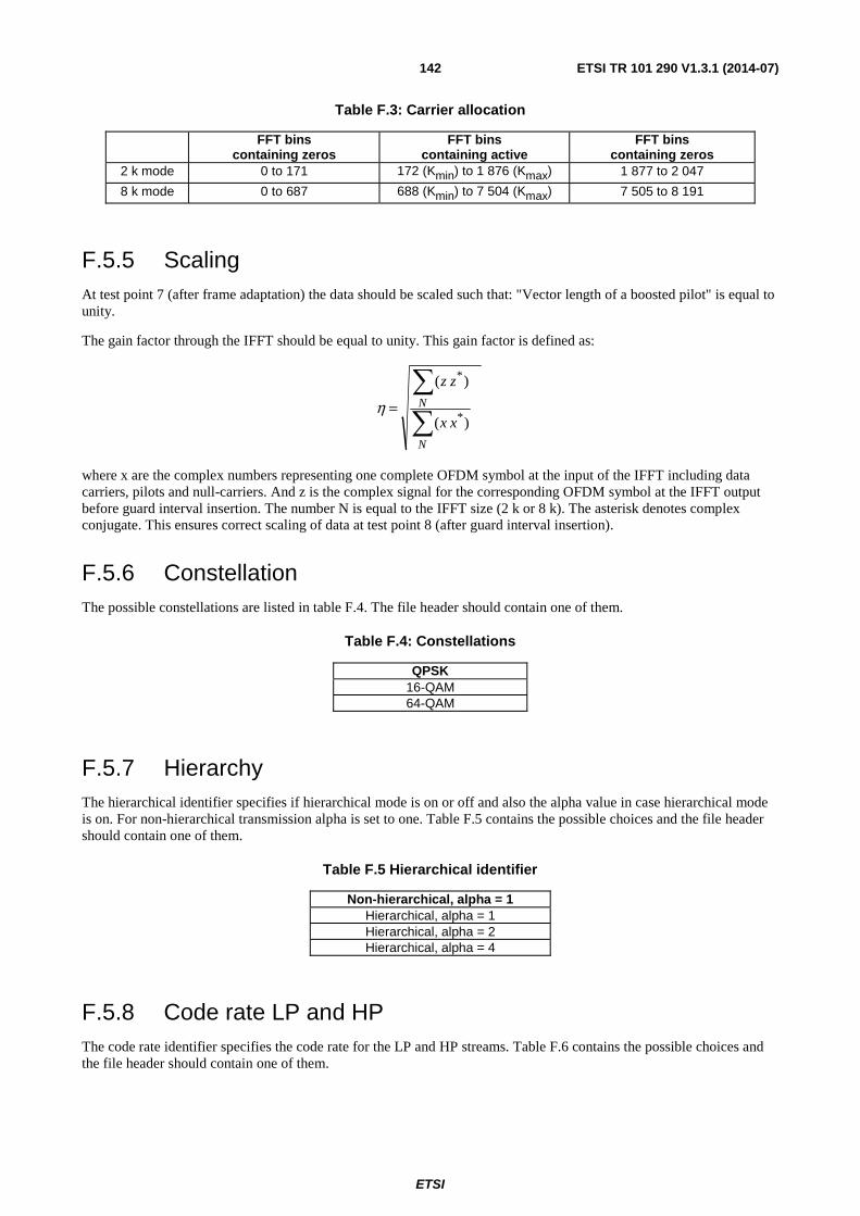
ETSI
ETSI TR 101 290 V1.3.1 (2014-07) 142
Table F.3: Carrier allocation
FFT bins containing zeros
FFT bins containing active
FFT bins containing zeros
2 k mode 0 to 171 172 (Kmin) to 1 876 (Kmax) 1 877 to 2 047
8 k mode 0 to 687 688 (Kmin) to 7 504 (Kmax) 7 505 to 8 191
F.5.5 Scaling At test point 7 (after frame adaptation) the data should be scaled such that: "Vector length of a boosted pilot" is equal to unity.
The gain factor through the IFFT should be equal to unity. This gain factor is defined as:
)(
)(
*
*
∑
∑=
N
N
xx
zz
η
where x are the complex numbers representing one complete OFDM symbol at the input of the IFFT including data carriers, pilots and null-carriers. And z is the complex signal for the corresponding OFDM symbol at the IFFT output before guard interval insertion. The number N is equal to the IFFT size (2 k or 8 k). The asterisk denotes complex conjugate. This ensures correct scaling of data at test point 8 (after guard interval insertion).
F.5.6 Constellation The possible constellations are listed in table F.4. The file header should contain one of them.
Table F.4: Constellations
QPSK 16-QAM 64-QAM
F.5.7 Hierarchy The hierarchical identifier specifies if hierarchical mode is on or off and also the alpha value in case hierarchical mode is on. For non-hierarchical transmission alpha is set to one. Table F.5 contains the possible choices and the file header should contain one of them.
Table F.5 Hierarchical identifier
Non-hierarchical, alpha = 1 Hierarchical, alpha = 1 Hierarchical, alpha = 2 Hierarchical, alpha = 4
F.5.8 Code rate LP and HP The code rate identifier specifies the code rate for the LP and HP streams. Table F.6 contains the possible choices and the file header should contain one of them.
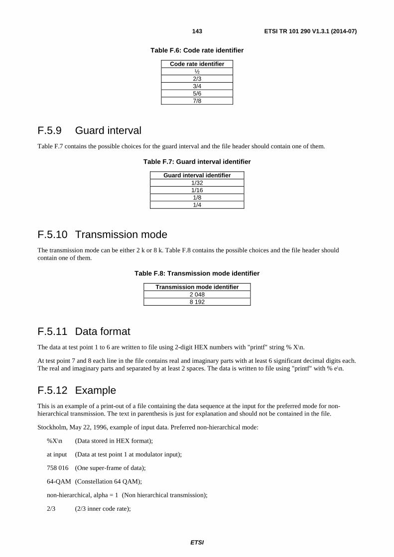
ETSI
ETSI TR 101 290 V1.3.1 (2014-07) 143
Table F.6: Code rate identifier
Code rate identifier ½
2/3 3/4 5/6 7/8
F.5.9 Guard interval Table F.7 contains the possible choices for the guard interval and the file header should contain one of them.
Table F.7: Guard interval identifier
Guard interval identifier 1/32 1/16 1/8 1/4
F.5.10 Transmission mode The transmission mode can be either 2 k or 8 k. Table F.8 contains the possible choices and the file header should contain one of them.
Table F.8: Transmission mode identifier
Transmission mode identifier 2 048 8 192
F.5.11 Data format The data at test point 1 to 6 are written to file using 2-digit HEX numbers with "printf" string % X\n.
At test point 7 and 8 each line in the file contains real and imaginary parts with at least 6 significant decimal digits each. The real and imaginary parts and separated by at least 2 spaces. The data is written to file using "printf" with % e\n.
F.5.12 Example This is an example of a print-out of a file containing the data sequence at the input for the preferred mode for non-hierarchical transmission. The text in parenthesis is just for explanation and should not be contained in the file.
Stockholm, May 22, 1996, example of input data. Preferred non-hierarchical mode:
%X\n (Data stored in HEX format);
at input (Data at test point 1 at modulator input);
758 016 (One super-frame of data);
64-QAM (Constellation 64 QAM);
non-hierarchical, alpha = 1 (Non hierarchical transmission);
2/3 (2/3 inner code rate);

ETSI
ETSI TR 101 290 V1.3.1 (2014-07) 144
0 (Don't care. Code rate LP);
1/32 (Guard interval = 1/32);
8 192 (8 k IFFT size);
47 (First data byte is sync byte 47 HEX);
00 (Rest of data).
ETSI
ETSI TR 101 290 V1.3.1 (2014-07) 145
Annex G: Theoretical background information on measurement techniques This informative annex presents a review of the theoretical background to the measurement techniques recommended in the present document. It is an attempt to gather the most relevant background information into one location, particularly for the benefit of engineers and technicians who are new to digital modulation techniques. It is hoped that it will provide a working knowledge of the theoretical and practical issues, particularly the potential sources of ambiguity and error, to help users of the present document make valid, accurate and repeatable measurements.
G.1 Overview The basic purpose of a digital transmission system is to transfer data from A to B with as few errors as possible. It follows that the fundamental measure of system quality is the transmission error rate.
The transmission error rate is usually measured as the Bit Error Rate (BER), however it can also be informative to consider the error rate of other transmission elements such as bytes, MPEG packets, or m-bit modulation symbols. In practice, although a certain guaranteed minimum BER performance may be a system implementation goal, the system BER alone is not a particularly informative measurement.
The most important figure of merit for any digital transmission system is the BER expressed as a function of the ratio of wanted information power to unwanted interference power (C/N). This is underlined by the fact that most of the measurements in the present document are built around this central theme of BER vs. C/N (or, equivalently, BER vs. Eb/N0).
There are measurements of the individual elements (power and BER measurements). There are measurements of the difference between theoretical and ideal performance (margin and degradation measurements). There are measurements intended to help identify the sources of transmission errors (interference, spectrum, jitter and I/Q measurements). There are measurements for monitoring the consequences of transmission errors at the system level (availability, error event logging).
G.2 RF/IF power ("carrier") When describing the Quadrature Amplitude Modulated (QAM) signals employed by DVB-C or the Quadrature Phase Shift Keying (QPSK) signals employed by DVB-S, it is common to refer to the modulated RF/IF signal as "carrier" (C), mainly to distinguish it from "signal" (S) which is generally used to refer to the baseband demodulated signal.
Strictly, it is incorrect to describe this signal as "carrier" because QAM and QPSK (which is equivalent to 4-state QAM) are suppressed carrier modulation schemes. For OFDM, with thousands of suppressed carriers and assorted pilot tones, the label "carrier" is even more inappropriate. This is why deliberately the expression "wanted information power" is used in the paragraph above, and why the parameter is referred to as "RF/IF power" in the present document.
However, it is clear that engineers will continue to use "carrier" as a convenient shorthand for this parameter, particularly when talking about the "carrier"-to-noise ratio. It seems futile to attempt to change this, so instead it is clearly defined what is meant by "carrier" in this context. Carrier, more accurately called RF/IF power, is the total power of the modulated RF/IF signal as would be measured by a thermal power sensor in the absence of any other signals (including noise).
For DVB compliant systems the QAM/QPSK passband spectrum is shaped by root raised cosine filtering with a roll-off factor alpha (α) of 0,15 for DVB-C systems, or 0,35 for DVB-S systems. For an ideal QAM/QPSK system this means that all the RF/IF power will lie in the frequency band:
( )
21)(
SCQAMOCC
ffBW ×+±= α
(G.1)

ETSI
ETSI TR 101 290 V1.3.1 (2014-07) 146
Equation G.1 defines the occupied bandwidth of the signal, where fC is the carrier frequency, fS is the symbol rate of
the modulation, and α is the filter roll-off factor. RF/IF power (or "carrier") is the total power in this "rectangular" bandwidth, that is, with no further filtering applied.
For OFDM systems the definition of occupied bandwidth is expressed differently because of the radically different modulation technique, however the principle is very similar. The OFDM "shoulders" are not considered to be wanted information power, and are not included in the RF/IF power calculation, even though the power does actually come out of the transmitter:
SPACINGOFDMOCC fnBW ×=)( (G.2)
where n = 6 817 (8 k mode) or 1 705 (2 k mode) and fSPACING = 1 116 Hz (8 k mode) or 4 464 Hz (2 k mode).
In a real multi-signal system (e.g. a live CATV network) measurement of the RF/IF power in a single channel requires a frequency selective technique. This could employ a thermal power metre preceded by a suitably calibrated channel filter, a spectrum analyser with band power measurement capability, or a measuring receiver. Depending on the measurement technique a filter may be required to exclude the "shoulders" of a single OFDM signal.
G.3 Noise level The noise level is the unwanted interference power present in the system when the wanted information power is removed. This is a less bounded quantity than the RF/IF power because there is no definitively "correct" bandwidth over which to measure the noise. The choice is to some extent arbitrary, but the "top three" choices are probably:
1) Channel bandwidth: In a channel based system such as a CATV network you could choose the channel bandwidth, for example 8 MHz, as the system noise bandwidth. This is considered by the DVB-MG to be inappropriate for C/N measurements in digital TV systems. It will result in misleadingly poor C/N ratios when the modulation symbol rate is low relative to the available channel bandwidth. It unnecessarily complicates conversion between C/N measurements made "in the channel " and "in the receiver " by introducing symbol rate dependent correction factors.
2) Symbol rate: For digital modulation employing Nyquist filtering split equally between the transmitter and receiver, the noise bandwidth of the receiver equals the symbol rate. This is considered by the DVB-MG to be appropriate for "in the receiver " C/N measurements of digital TV systems since this reflects the amount of noise entering the receiver independent of symbol rate.
3) The occupied bandwidth: For digital modulation employing Nyquist filtering the occupied bandwidth of the modulated signal is (1 + α) × fS. This is considered by the DVB-MG to be appropriate for "in the channel "
C/N measurements of digital TV systems since it exactly covers the transmitted spectrum, independent of symbol rate.
The DVB-MG have chosen occupied bandwidth, as defined by equation G.1, as the standard definition of noise bandwidth in DVB-C and DVB-S systems. This is primarily because "in the channel " C/N is considered to be the fundamental measurement, but also because a simple correction factor can be applied to determine the equivalent "in the receiver " C/N value.
The other possibility that should be mentioned is to assume that the noise power is evenly distributed across the frequency spectrum of interest and so can be described by a single noise power density value (N0) which is the noise
power present in a 1 Hz bandwidth. From this, the noise power present in any given system noise power bandwidth (BWSYS) can be obtained by simple multiplication:
SYSBWNN ×= 0 (G.3)
By talking in terms of N0 we are freed from the need to define a noise bandwidth, but we are making an assumption that
the noise power spectrum is flat across the bandwidth of interest.

ETSI
ETSI TR 101 290 V1.3.1 (2014-07) 147
G.4 Energy-per-bit (Eb) Trying to commission a DVB system against tight deadlines, Energy-per-bit (Eb) seems to be a rather academic
concept, particularly since the directly measurable quantity is RF power.
However, it is useful to understand Eb, even if only to avoid confusion when it appears in technical specifications or
discussions. Historically, use of Eb arises from information theory and as part of an academic desire to normalize the
performance of different modulation formats and coding schemes for comparative purposes.
The Energy-per-bit is the energy expended in transmitting each single bit of information. Eb is of little practical use on
its own, it is most useful in the context of a graph of BER vs. the Eb/N0 ratio - the well known "waterfall curve" (see
figures G.1 and G.2).
By normalizing to an Eb/N0 ratio on the X axis, the relative performance of various complexities of digital modulation
and channel coding can be compared because the scaling effects of actual signal and noise powers, number of bits-per-symbol and symbol rate are removed. It is then simply a case of comparing the bit error probability for a given ratio.
Energy-per-bit can be easily translated to carrier power. Power is energy-per-second. Which can be expanded to energy-per-bit, times bits-per-symbol, times symbols-per-second. Expressed algebraically we get:
( ) Sb fMEC ××= 2log (G.4)
G.5 C/N ratio and Eb/No ratio The parameters that can be directly measured are RF/IF or "carrier" power (C) and noise power in a certain bandwidth (N). From these measurements we can immediately compute the C/N ratio.
With the equations above, knowledge of the other parameters (e.g. fS ) and a little algebra we can also arrive at an
equivalent Eb/N0 ratio.
G.6 Practical application of the measurements At this point it seems that C/N (or Eb/N0) is defined, and indeed it is from an algebraic perspective.
However, there is scope for endless confusion in applying these simple formulae unless the user is very clear about where the C/N or Eb/N0 ratio is being measured, and what values are being used for the subordinate parameters, most
particularly the system noise bandwidth.
C/N (or Eb/N0) can be measured "in the channel" or "in the receiver". The meaning of "in the channel" is fairly self-
evident, "in the receiver" may need further explanation.
There are typically three filtering processes present in a receiver. The first (which is optional) is a relatively broadband tuneable pre-selection simply to reduce the power presented to the receiver RF front-end. The second, usually applied at an IF, is a high-order bandpass channel selection filter to extract the desired signal with (ideally) no modification of the signal spectrum. The third is the root-raised cosine Nyquist filtering, commonly implemented in the low pass filters following the I/Q demodulation.
For theoretical simplicity we assume that the receiver's bandwidth and band shape are defined totally by the low-pass root-raised cosine filters because the intended purpose of the other RF/IF filters is only signal pre-selection. So we can model the receiver as a broadband receiver with a root-raised cosine passband filter followed by I/Q demodulation.
With this in mind, "in the receiver" can be seen to mean "after the bandwidth and band shape modifying effects of the receiver Nyquist filters has been taken into account".
Whether artificially generating a specific C/N ratio or just measuring the existing C/N ratio it is important to understand the difference between the "in the channel" and "in the receiver" nodes.

ETSI
ETSI TR 101 290 V1.3.1 (2014-07) 148
On a more practical note, graphing the BER performance of a receiver versus Eb/N0 removes the ambiguity introduced
by varying noise bandwidth. If we use the "in the channel" Eb value then we get a certain BER curve, if we use the
slightly lower "in the receiver" Eb value then the Eb/N0 ratio is slightly poorer for the same BER, the curve moves to
the left (closer to the theoretical curve) and the implementation loss decreases because the loss due to the receive filters is not included. An example may help to explain this.
G.7 Example Creation of a signal with a specific C/N ratio in order to test the performance of an Integrated Receiver Decoder (IRD), or perhaps to degrade an incoming RF/IF signal to a specific C/N ratio in order to establish the noise margin.
To do this, add broadband white Gaussian noise "in the channel " to the relatively noise free RF/IF signal. Measure (or compute) the carrier power and then adjust the noise power density to give the required noise power in the selected noise power bandwidth.
Taking the following QAM system parameters as an example:
Symbol rate: fS = 6,875 MHz;
Filter roll-off: α = 0,15;
System noise bandwidth: BWNOISE = 8 MHz;
Constellation size: M = 64;
Carrier power (in dB): C = -25 dBm.
then:
25−=C dBm
( )( ) 15,101loglog10 210 −=××−= Sb fMCE dBm
If a C/N ratio of 23 dB is wanted, then:
00,48−=⎟⎠
⎞⎜⎝
⎛−=dBN
CCN dBm
( ) 03,117log10 100 −=×−= NOISEBWNN dBm
So the ratio of Carrier-to-Noise applied in an 8 MHz system bandwidth at RF/IF can be described as:
00,23=N
CdB
88,150
=N
Eb dB
This signal is then passed through the receiver root-raised cosine filters. The equivalent noise bandwidth of a bandpass root-raised cosine filter is equal to the symbol rate fS. The noise power originally defined in an 8 MHz system
bandwidth is reduced accordingly:
66,48log10 10 −=⎟⎟⎠
⎞⎜⎜⎝
⎛×+=
NOISE
SREC BW
fNN
dB (G.5)
The noise power density N0 is unchanged by the receive filter:
N0(REC) = N0 = -117,03 dBm.
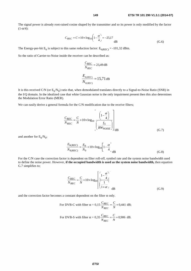
ETSI
ETSI TR 101 290 V1.3.1 (2014-07) 149
The signal power is already root-raised cosine shaped by the transmitter and so its power is only modified by the factor (1-α/4):
17,25
41log10 10 −=⎟
⎠
⎞⎜⎝
⎛ −×+= αCCREC
dB (G.6)
The Energy-per-bit Eb is subject to this same reduction factor: Eb(REC) = -101,32 dBm.
So the ratio of Carrier-to-Noise inside the receiver can be described as:
49,23=REC
REC
N
CdB
71,15)(0
)( =REC
RECb
N
EdB
It is this received C/N (or Eb/N0) ratio that, when demodulated translates directly to a Signal-to-Noise Ratio (SNR) in
the I/Q domain. In the idealized case that white Gaussian noise is the only impairment present then this also determines the Modulation Error Ratio (MER).
We can easily derive a general formula for the C/N modification due to the receive filters;
⎥⎥⎥⎥⎥
⎦
⎤
⎢⎢⎢⎢⎢
⎣
⎡
⎟⎟⎠
⎞⎜⎜⎝
⎛
⎟⎠
⎞⎜⎝
⎛ −×+=
NOISE
SREC
REC
BW
fN
C
N
C 41
log10 10
α
dB (G.7)
and another for Eb/N0;
⎥⎦
⎤⎢⎣
⎡ −×+=4
1log10 100)(0
)( αN
E
N
E b
REC
RECb
dB (G.8)
For the C/N case the correction factor is dependent on filter roll-off, symbol rate and the system noise bandwidth used to define the noise power. However, if the occupied bandwidth is used as the system noise bandwidth, then equation G.7 simplifies to;
⎥⎥⎥⎥
⎦
⎤
⎢⎢⎢⎢
⎣
⎡
⎟⎠
⎞⎜⎝
⎛
+
⎟⎠
⎞⎜⎝
⎛ −×+=
α
α
1
14
1log10 10N
C
N
C
REC
REC
dB (G.9)
and the correction factor becomes a constant dependent on the filter α only.
For DVB-C with filter α = 0,15 441,0+=N
C
N
C
REC
REC dB;
For DVB-S with filter α = 0,35 906,0+=N
C
N
C
REC
REC dB.
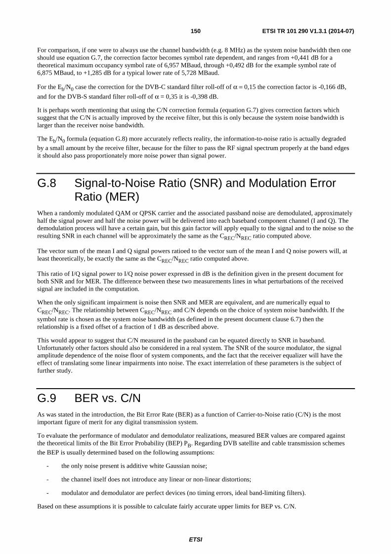
ETSI
ETSI TR 101 290 V1.3.1 (2014-07) 150
For comparison, if one were to always use the channel bandwidth (e.g. 8 MHz) as the system noise bandwidth then one should use equation G.7, the correction factor becomes symbol rate dependent, and ranges from +0,441 dB for a theoretical maximum occupancy symbol rate of 6,957 MBaud, through +0,492 dB for the example symbol rate of 6,875 MBaud, to +1,285 dB for a typical lower rate of 5,728 MBaud.
For the Eb/N0 case the correction for the DVB-C standard filter roll-off of α = 0,15 the correction factor is -0,166 dB,
and for the DVB-S standard filter roll-off of α = 0,35 it is -0,398 dB.
It is perhaps worth mentioning that using the C/N correction formula (equation G.7) gives correction factors which suggest that the C/N is actually improved by the receive filter, but this is only because the system noise bandwidth is larger than the receiver noise bandwidth.
The Eb/N0 formula (equation G.8) more accurately reflects reality, the information-to-noise ratio is actually degraded
by a small amount by the receive filter, because for the filter to pass the RF signal spectrum properly at the band edges it should also pass proportionately more noise power than signal power.
G.8 Signal-to-Noise Ratio (SNR) and Modulation Error Ratio (MER)
When a randomly modulated QAM or QPSK carrier and the associated passband noise are demodulated, approximately half the signal power and half the noise power will be delivered into each baseband component channel (I and Q). The demodulation process will have a certain gain, but this gain factor will apply equally to the signal and to the noise so the resulting SNR in each channel will be approximately the same as the CREC/NREC ratio computed above.
The vector sum of the mean I and Q signal powers ratioed to the vector sum of the mean I and Q noise powers will, at least theoretically, be exactly the same as the CREC/NREC ratio computed above.
This ratio of I/Q signal power to I/Q noise power expressed in dB is the definition given in the present document for both SNR and for MER. The difference between these two measurements lines in what perturbations of the received signal are included in the computation.
When the only significant impairment is noise then SNR and MER are equivalent, and are numerically equal to CREC/NREC. The relationship between CREC/NREC and C/N depends on the choice of system noise bandwidth. If the
symbol rate is chosen as the system noise bandwidth (as defined in the present document clause 6.7) then the relationship is a fixed offset of a fraction of 1 dB as described above.
This would appear to suggest that C/N measured in the passband can be equated directly to SNR in baseband. Unfortunately other factors should also be considered in a real system. The SNR of the source modulator, the signal amplitude dependence of the noise floor of system components, and the fact that the receiver equalizer will have the effect of translating some linear impairments into noise. The exact interrelation of these parameters is the subject of further study.
G.9 BER vs. C/N As was stated in the introduction, the Bit Error Rate (BER) as a function of Carrier-to-Noise ratio (C/N) is the most important figure of merit for any digital transmission system.
To evaluate the performance of modulator and demodulator realizations, measured BER values are compared against the theoretical limits of the Bit Error Probability (BEP) PB. Regarding DVB satellite and cable transmission schemes
the BEP is usually determined based on the following assumptions:
- the only noise present is additive white Gaussian noise;
- the channel itself does not introduce any linear or non-linear distortions;
- modulator and demodulator are perfect devices (no timing errors, ideal band-limiting filters).
Based on these assumptions it is possible to calculate fairly accurate upper limits for BEP vs. C/N.
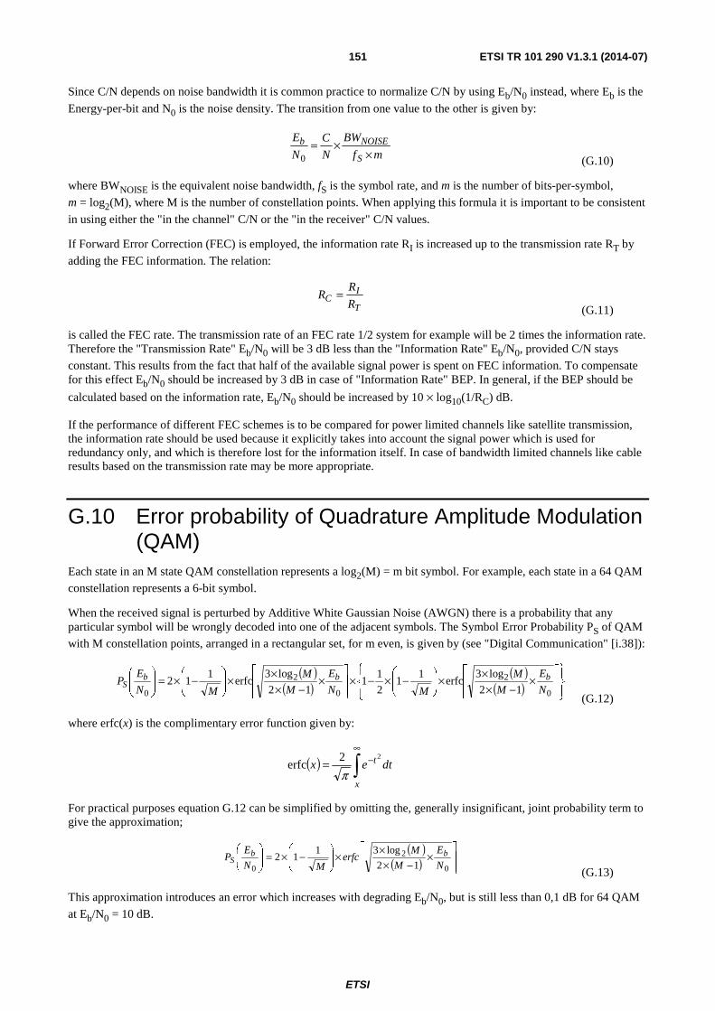
ETSI
ETSI TR 101 290 V1.3.1 (2014-07) 151
Since C/N depends on noise bandwidth it is common practice to normalize C/N by using Eb/N0 instead, where Eb is the
Energy-per-bit and N0 is the noise density. The transition from one value to the other is given by:
mf
BW
N
C
N
E
S
NOISEb
××=
0 (G.10)
where BWNOISE is the equivalent noise bandwidth, fS is the symbol rate, and m is the number of bits-per-symbol,
m = log2(M), where M is the number of constellation points. When applying this formula it is important to be consistent
in using either the "in the channel" C/N or the "in the receiver" C/N values.
If Forward Error Correction (FEC) is employed, the information rate RI is increased up to the transmission rate RT by
adding the FEC information. The relation:
T
IC R
RR =
(G.11)
is called the FEC rate. The transmission rate of an FEC rate 1/2 system for example will be 2 times the information rate. Therefore the "Transmission Rate" Eb/N0 will be 3 dB less than the "Information Rate" Eb/N0, provided C/N stays
constant. This results from the fact that half of the available signal power is spent on FEC information. To compensate for this effect Eb/N0 should be increased by 3 dB in case of "Information Rate" BEP. In general, if the BEP should be
calculated based on the information rate, Eb/N0 should be increased by 10 × log10(1/RC) dB.
If the performance of different FEC schemes is to be compared for power limited channels like satellite transmission, the information rate should be used because it explicitly takes into account the signal power which is used for redundancy only, and which is therefore lost for the information itself. In case of bandwidth limited channels like cable results based on the transmission rate may be more appropriate.
G.10 Error probability of Quadrature Amplitude Modulation (QAM)
Each state in an M state QAM constellation represents a log2(M) = m bit symbol. For example, each state in a 64 QAM
constellation represents a 6-bit symbol.
When the received signal is perturbed by Additive White Gaussian Noise (AWGN) there is a probability that any particular symbol will be wrongly decoded into one of the adjacent symbols. The Symbol Error Probability PS of QAM
with M constellation points, arranged in a rectangular set, for m even, is given by (see "Digital Communication" [i.38]):
( )( )
( )( ) ⎪⎭
⎪⎬⎫
⎪⎩
⎪⎨⎧
⎥⎥⎦
⎤
⎢⎢⎣
⎡×
−×××⎟⎟
⎠
⎞⎜⎜⎝
⎛−×−×
⎥⎥⎦
⎤
⎢⎢⎣
⎡×
−×××⎟⎟
⎠
⎞⎜⎜⎝
⎛−×=⎟⎟
⎠
⎞⎜⎜⎝
⎛
0
2
0
2
0 12
log3erfc
11
2
11
12
log3erfc
112
N
E
M
M
MN
E
M
M
MN
EP bbb
S
(G.12)
where erfc(x) is the complimentary error function given by:
( ) ∫∞
−=x
t dtex22
erfcπ
For practical purposes equation G.12 can be simplified by omitting the, generally insignificant, joint probability term to give the approximation;
( )( ) ⎥
⎥⎦
⎤
⎢⎢⎣
⎡×
−××
×⎟⎟⎠
⎞⎜⎜⎝
⎛−×=⎟
⎟⎠
⎞⎜⎜⎝
⎛
0
2
0 12
log3112
N
E
M
Merfc
MN
EP bb
S
(G.13)
This approximation introduces an error which increases with degrading Eb/N0, but is still less than 0,1 dB for 64 QAM
at Eb/N0 = 10 dB.
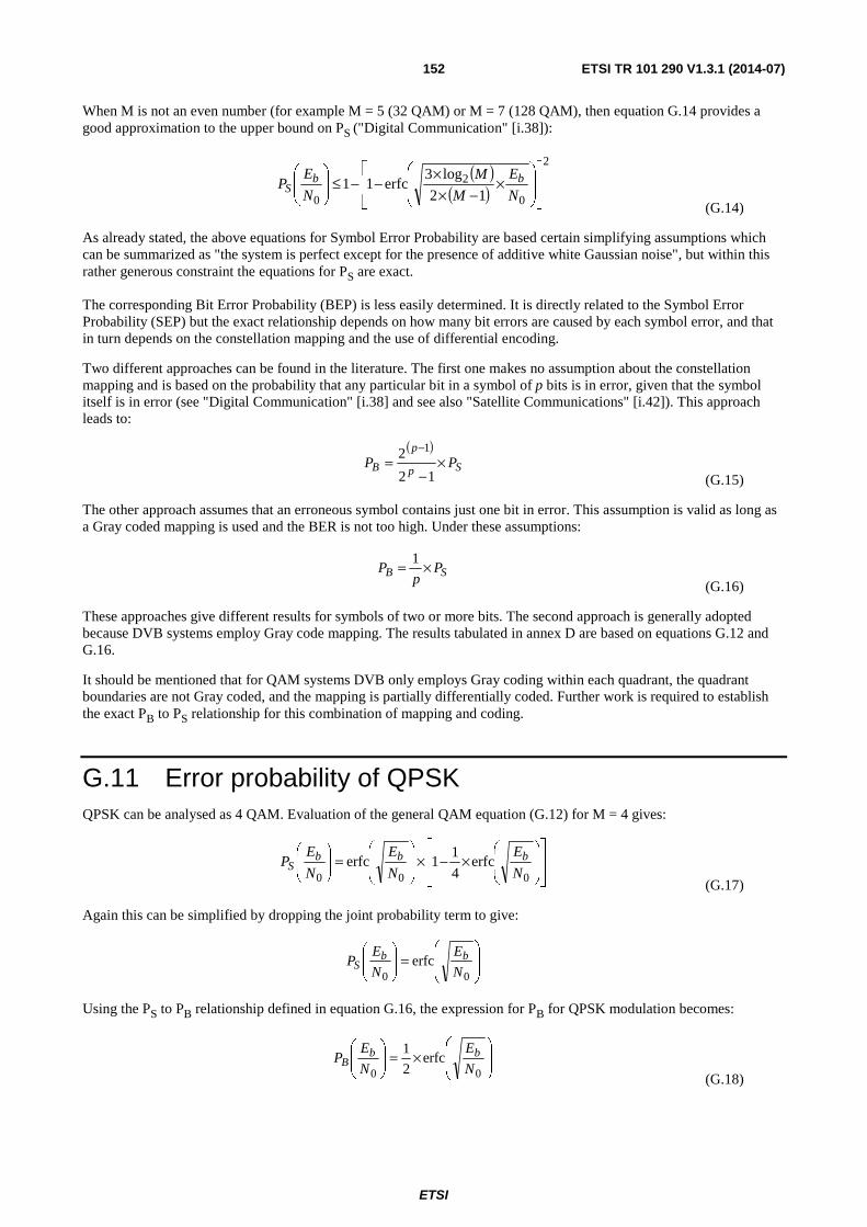
ETSI
ETSI TR 101 290 V1.3.1 (2014-07) 152
When M is not an even number (for example M = 5 (32 QAM) or M = 7 (128 QAM), then equation G.14 provides a good approximation to the upper bound on PS ("Digital Communication" [i.38]):
( )( )
2
0
2
0 12
log3erfc11
⎥⎥
⎦
⎤
⎢⎢
⎣
⎡
⎟⎟
⎠
⎞
⎜⎜
⎝
⎛×
−××
−−≤⎟⎟⎠
⎞⎜⎜⎝
⎛
N
E
M
M
N
EP bb
S
(G.14)
As already stated, the above equations for Symbol Error Probability are based certain simplifying assumptions which can be summarized as "the system is perfect except for the presence of additive white Gaussian noise", but within this rather generous constraint the equations for PS are exact.
The corresponding Bit Error Probability (BEP) is less easily determined. It is directly related to the Symbol Error Probability (SEP) but the exact relationship depends on how many bit errors are caused by each symbol error, and that in turn depends on the constellation mapping and the use of differential encoding.
Two different approaches can be found in the literature. The first one makes no assumption about the constellation mapping and is based on the probability that any particular bit in a symbol of p bits is in error, given that the symbol itself is in error (see "Digital Communication" [i.38] and see also "Satellite Communications" [i.42]). This approach leads to:
( )Sp
p
B PP ×−
=−
12
2 1
(G.15)
The other approach assumes that an erroneous symbol contains just one bit in error. This assumption is valid as long as a Gray coded mapping is used and the BER is not too high. Under these assumptions:
SB P
pP ×= 1
(G.16)
These approaches give different results for symbols of two or more bits. The second approach is generally adopted because DVB systems employ Gray code mapping. The results tabulated in annex D are based on equations G.12 and G.16.
It should be mentioned that for QAM systems DVB only employs Gray coding within each quadrant, the quadrant boundaries are not Gray coded, and the mapping is partially differentially coded. Further work is required to establish the exact PB to PS relationship for this combination of mapping and coding.
G.11 Error probability of QPSK QPSK can be analysed as 4 QAM. Evaluation of the general QAM equation (G.12) for M = 4 gives:
⎥⎥
⎦
⎤
⎢⎢
⎣
⎡
⎟⎟
⎠
⎞
⎜⎜
⎝
⎛×−×
⎟⎟
⎠
⎞
⎜⎜
⎝
⎛=⎟
⎟⎠
⎞⎜⎜⎝
⎛
000erfc
4
11erfc
N
E
N
E
N
EP bbb
S
(G.17)
Again this can be simplified by dropping the joint probability term to give:
⎟⎟
⎠
⎞
⎜⎜
⎝
⎛=⎟
⎟⎠
⎞⎜⎜⎝
⎛
00erfc
N
E
N
EP bb
S
Using the PS to PB relationship defined in equation G.16, the expression for PB for QPSK modulation becomes:
⎟⎟
⎠
⎞
⎜⎜
⎝
⎛×=⎟
⎟⎠
⎞⎜⎜⎝
⎛
00erfc
2
1
N
E
N
EP bb
B
(G.18)
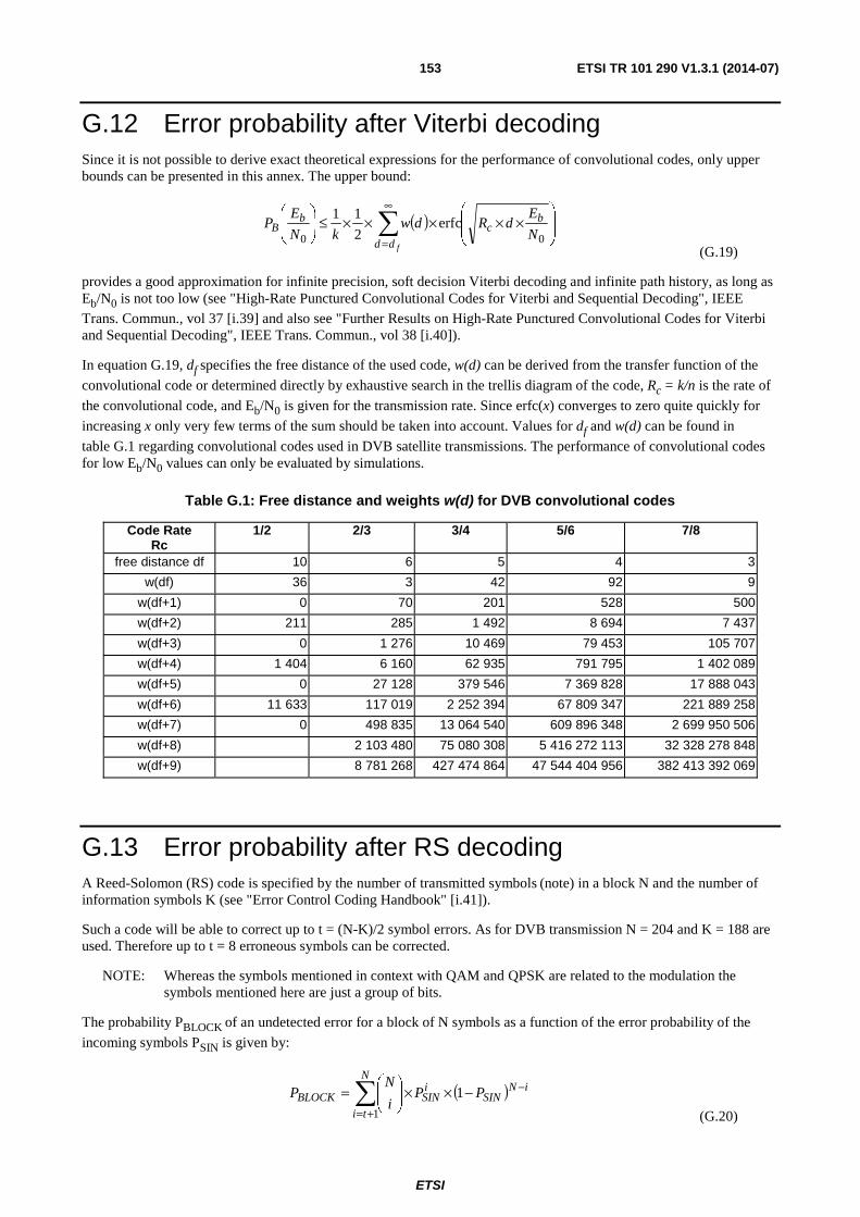
ETSI
ETSI TR 101 290 V1.3.1 (2014-07) 153
G.12 Error probability after Viterbi decoding Since it is not possible to derive exact theoretical expressions for the performance of convolutional codes, only upper bounds can be presented in this annex. The upper bound:
( )⎟⎟
⎠
⎞
⎜⎜
⎝
⎛×××××≤⎟
⎟⎠
⎞⎜⎜⎝
⎛∑
∞
= 00erfc
2
11
N
EdRdw
kN
EP b
c
dd
bB
f (G.19)
provides a good approximation for infinite precision, soft decision Viterbi decoding and infinite path history, as long as Eb/N0 is not too low (see "High-Rate Punctured Convolutional Codes for Viterbi and Sequential Decoding", IEEE
Trans. Commun., vol 37 [i.39] and also see "Further Results on High-Rate Punctured Convolutional Codes for Viterbi and Sequential Decoding", IEEE Trans. Commun., vol 38 [i.40]).
In equation G.19, df specifies the free distance of the used code, w(d) can be derived from the transfer function of the
convolutional code or determined directly by exhaustive search in the trellis diagram of the code, Rc = k/n is the rate of
the convolutional code, and Eb/N0 is given for the transmission rate. Since erfc(x) converges to zero quite quickly for
increasing x only very few terms of the sum should be taken into account. Values for df and w(d) can be found in
table G.1 regarding convolutional codes used in DVB satellite transmissions. The performance of convolutional codes for low Eb/N0 values can only be evaluated by simulations.
Table G.1: Free distance and weights w(d) for DVB convolutional codes
Code Rate Rc
1/2 2/3 3/4 5/6 7/8
free distance df 10 6 5 4 3
w(df) 36 3 42 92 9
w(df+1) 0 70 201 528 500
w(df+2) 211 285 1 492 8 694 7 437
w(df+3) 0 1 276 10 469 79 453 105 707
w(df+4) 1 404 6 160 62 935 791 795 1 402 089
w(df+5) 0 27 128 379 546 7 369 828 17 888 043
w(df+6) 11 633 117 019 2 252 394 67 809 347 221 889 258
w(df+7) 0 498 835 13 064 540 609 896 348 2 699 950 506
w(df+8) 2 103 480 75 080 308 5 416 272 113 32 328 278 848
w(df+9) 8 781 268 427 474 864 47 544 404 956 382 413 392 069
G.13 Error probability after RS decoding A Reed-Solomon (RS) code is specified by the number of transmitted symbols (note) in a block N and the number of information symbols K (see "Error Control Coding Handbook" [i.41]).
Such a code will be able to correct up to t = (N-K)/2 symbol errors. As for DVB transmission N = 204 and K = 188 are used. Therefore up to t = 8 erroneous symbols can be corrected.
NOTE: Whereas the symbols mentioned in context with QAM and QPSK are related to the modulation the symbols mentioned here are just a group of bits.
The probability PBLOCK of an undetected error for a block of N symbols as a function of the error probability of the
incoming symbols PSIN is given by:
( )∑+=
−−××⎟⎟⎠
⎞⎜⎜⎝
⎛=
N
ti
iNSIN
iSINBLOCK PP
i
NP
1
1
(G.20)

ETSI
ETSI TR 101 290 V1.3.1 (2014-07) 154
From this expression the probability:
( ) iNSIN
iSIN
N
ti
iS PPi
N
NP −
+=
−××⎟⎟⎠
⎞⎜⎜⎝
⎛××= ∑ 1
1
1
β (G.21)
of a symbol error can be derived, where βi is the average number of symbol errors remaining in the received block
given that the channel caused i symbol errors. Of course βi = 0 for i ≤ t. When i > t, βi can be bounded by considering
that if more than "t" errors occur, a decoder which can correct a maximum of "t" errors will at best correct "t" of the errors and at worst add "t" errors. So:
titi i +≤≤− β (G.22)
is the possible range for βi. A good approximation is βi = i but also βi = t + i is used, which can be regarded as an upper
limit. From G.21 the BEP can be calculated by using G.15 or G.16.
G.14 BEP vs. C/N for DVB cable transmission For DVB transmission in cable networks, QAM-M systems with M = 16, 32 and 64 are specified. To evaluate the BEP after RS decoding, the following steps should be done:
a) calculate the SEP after QAM demodulation by using (G.12) or (G.14);
b) transform the SEP into a BEP by applying (G.15) or (G.16) to the SEP with p = m;
c) transform the resulting BEP into a SEP with p = 8 by using (G.15) or (G.16);
d) use (G.21) to calculate the SEP PS after RS decoding;
e) apply (G.15) or (G.16) to PS with p = 8 to determine the final BEP;
f) if the BEP should be based on the information rate, shift the curve by:
- 10 × log10(204/188) = 0,35 dB to the right.
If just the BEP before Reed-Solomon is needed, only the first two steps are necessary. In this case there is no difference between information rate and transmission rate. All bits are regarded as information bits.
The limits before and after Reed-Solomon decoding for M = 64, βi = i and Eb, based on the transmission rate, are
presented in figure G.1.
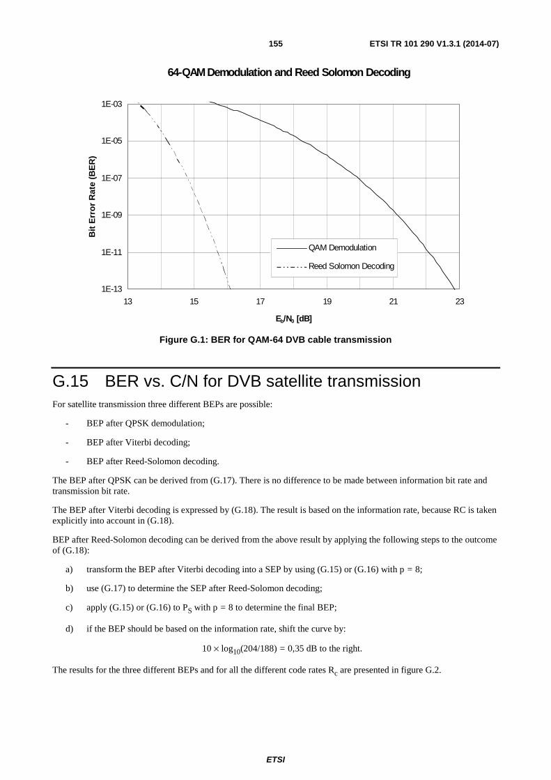
ETSI
ETSI TR 101 290 V1.3.1 (2014-07) 155
64-QAM Demodulation and Reed Solomon Decoding
1E-13
1E-11
1E-09
1E-07
1E-05
1E-03
13 15 17 19 21 23
Eb/N0 [dB]
Bit
Err
or
Rat
e (B
ER
)
QAM Demodulation
Reed Solomon Decoding
Figure G.1: BER for QAM-64 DVB cable transmission
G.15 BER vs. C/N for DVB satellite transmission For satellite transmission three different BEPs are possible:
- BEP after QPSK demodulation;
- BEP after Viterbi decoding;
- BEP after Reed-Solomon decoding.
The BEP after QPSK can be derived from (G.17). There is no difference to be made between information bit rate and transmission bit rate.
The BEP after Viterbi decoding is expressed by (G.18). The result is based on the information rate, because RC is taken explicitly into account in (G.18).
BEP after Reed-Solomon decoding can be derived from the above result by applying the following steps to the outcome of (G.18):
a) transform the BEP after Viterbi decoding into a SEP by using (G.15) or (G.16) with p = 8;
b) use (G.17) to determine the SEP after Reed-Solomon decoding;
c) apply (G.15) or (G.16) to PS with p = 8 to determine the final BEP;
d) if the BEP should be based on the information rate, shift the curve by:
10 × log10(204/188) = 0,35 dB to the right.
The results for the three different BEPs and for all the different code rates Rc are presented in figure G.2.

ETSI
ETSI TR 101 290 V1.3.1 (2014-07) 156
QPSK Demodulation, Viterbi and Reed Solomon Decoding
1E-12
1E-10
1E-08
1E-06
1E-04
1E-02
0 2 4 6 8 10 12 14
Eb/N0 [dB]
Bit
Err
or
Rat
e (B
ER
)
1/22/3
3/47/8
5/6
QPSK-Demodulation
Viterbi
Reed-Solomon 1/2
2/33/4
7/85/6
Figure G.2: BER for DVB satellite transmission
Since it is common practice in satellite transmission to refer the results to the information rates the curves for BEP after Reed-Solomon decoding have been shifted accordingly. The expression (G.19) is only valid for low error rates. Despite the fact that for decreasing Eb/N0 the BER should converge to 1/2 the results according to (G.19) will posses a
singularity for Eb/N0 = 0. This behaviour is especially pronounced for Rc = 7/8, where the assumption of a low error
rate is not fulfilled above a BEP of 10-4.
G.16 Adding noise to a noisy signal In a practical situation where we deliberately add noise to real signal in order to create a specific C/N ratio for measurement purposes, it is important to realize that there are two fundamental assumptions implicit in this technique.
The first assumption is that the input signal has a high C/N ratio and can, for practical purposes, be regarded as carrier only. The second assumption is that the input signal has a considerably better C/N ratio than the C/N ratio we wish to generate. In practice we may be adding noise to an already noisy signal, and in this case there are accuracy issues related to the above assumptions that should be considered.
First consider how noise is typically added to a signal. Figure G.3 gives a simplified block diagram.
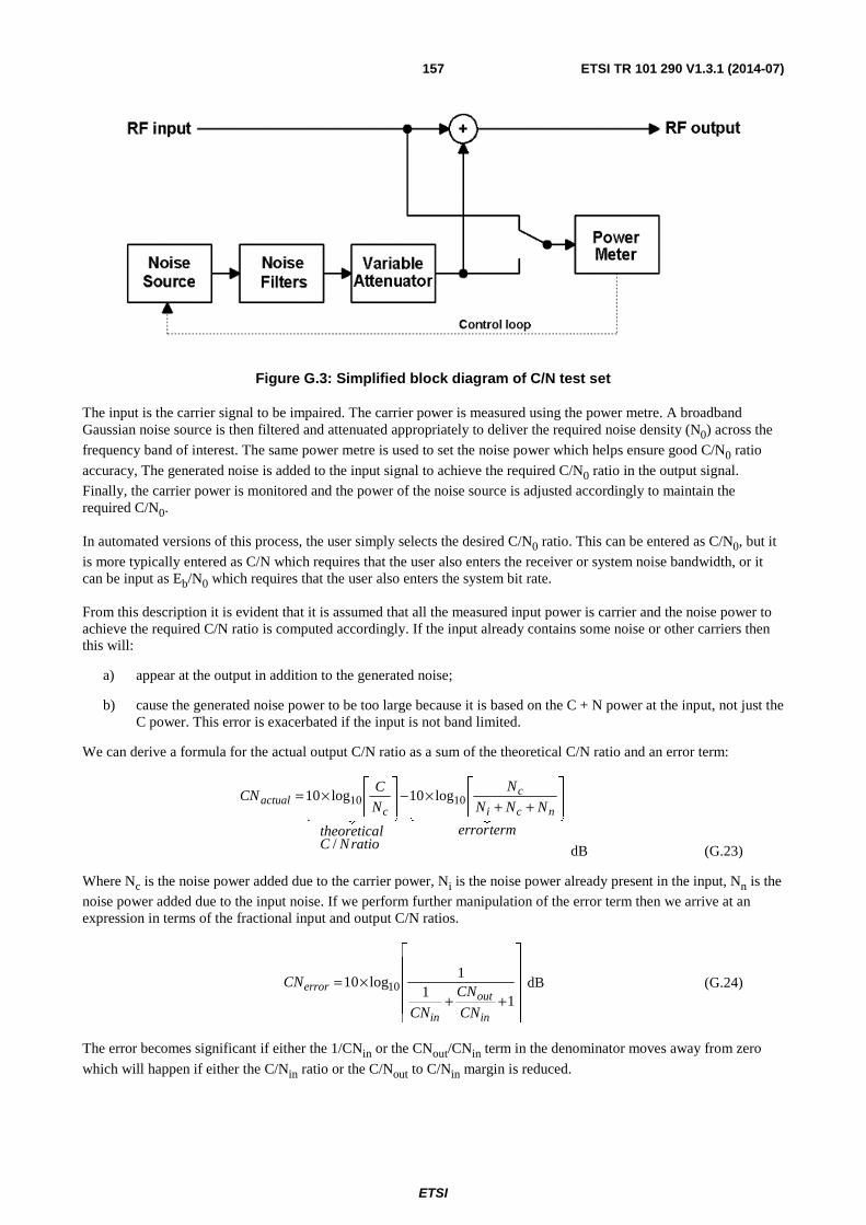
ETSI
ETSI TR 101 290 V1.3.1 (2014-07) 157
Figure G.3: Simplified block diagram of C/N test set
The input is the carrier signal to be impaired. The carrier power is measured using the power metre. A broadband Gaussian noise source is then filtered and attenuated appropriately to deliver the required noise density (N0) across the
frequency band of interest. The same power metre is used to set the noise power which helps ensure good C/N0 ratio
accuracy, The generated noise is added to the input signal to achieve the required C/N0 ratio in the output signal.
Finally, the carrier power is monitored and the power of the noise source is adjusted accordingly to maintain the required C/N0.
In automated versions of this process, the user simply selects the desired C/N0 ratio. This can be entered as C/N0, but it
is more typically entered as C/N which requires that the user also enters the receiver or system noise bandwidth, or it can be input as Eb/N0 which requires that the user also enters the system bit rate.
From this description it is evident that it is assumed that all the measured input power is carrier and the noise power to achieve the required C/N ratio is computed accordingly. If the input already contains some noise or other carriers then this will:
a) appear at the output in addition to the generated noise;
b) cause the generated noise power to be too large because it is based on the C + N power at the input, not just the C power. This error is exacerbated if the input is not band limited.
We can derive a formula for the actual output C/N ratio as a sum of the theoretical C/N ratio and an error term:
4444 34444 2144 344 21
termerror
NNN
N
ratioNCltheoretica
N
CCN
nci
c
cactual ⎥
⎦
⎤⎢⎣
⎡
++×−⎥
⎦
⎤⎢⎣
⎡×= 1010 log10
/
log10
dB (G.23)
Where Nc is the noise power added due to the carrier power, Ni is the noise power already present in the input, Nn is the
noise power added due to the input noise. If we perform further manipulation of the error term then we arrive at an expression in terms of the fractional input and output C/N ratios.
⎥⎥⎥⎥
⎦
⎤
⎢⎢⎢⎢
⎣
⎡
++×=
11
1log10 10
in
out
in
error
CN
CN
CN
CN dB (G.24)
The error becomes significant if either the 1/CNin or the CNout/CNin term in the denominator moves away from zero
which will happen if either the C/Nin ratio or the C/Nout to C/Nin margin is reduced.

ETSI
ETSI TR 101 290 V1.3.1 (2014-07) 158
The present document gives a minimum value of 15 dB for the C/Nin ratio and for the C/Nout to C/Nin margin as a
guideline figure. To meet this condition in satellite systems it is necessary to use a sufficiently large dish to get the required C/N ratio. A received C/N ratio of 20 dB or more is desirable.
Alternatively, it is possible to work with higher noise signals if it is possible to measure the carrier and noise power accurately, for example by measuring carrier plus noise then switching off the carrier and measuring noise only. Equation G.23 can then be used to compensate for the errors due to the input noise.

ETSI
ETSI TR 101 290 V1.3.1 (2014-07) 159
Annex H: Void

ETSI
ETSI TR 101 290 V1.3.1 (2014-07) 160
Annex I: PCR related measurements Void.
ETSI
ETSI TR 101 290 V1.3.1 (2014-07) 161
Annex J: Bitrate related measurements
J.1 Introduction
J.1.1 Purpose of bitrate measurement This annex is intended to clarify a bitrate measurement technique which will allow different vendors of equipment to display the same bitrate value on their equipment when they analyse the same transport stream.
The measurement technique in this specification should be applicable to the whole transport stream as well as its individual components. This should allow displays of transport stream information such as the traditional "bouncing bars" statistical multiplex display to be shown consistently on different equipment. This display is intended to dynamically show the different allocation of bitrate between different services. The intention is that the measurement should be stand-alone and non-intrusive.
The measurement technique should also be easy to implement so that cost-effective designs can be introduced to large MPTS systems. It should also be scalable so that as extra precision is required, a more expensive device can be built using the same principles.
The technique is also appropriate for non Transport Stream system, but the use in such systems is outside the scope of the present document.
J.1.2 User Rate versus Multiplex Rate MPEG-2 transport streams are comprised of many different elements including but not limited to multiple compressed video and audio streams, teletext, table data, conditional access streams, IP data, and other private data. Each of these individual elements and the overall transport stream have data rates associated with them. The data rates can be time varying for the individual elements and the overall stream.
It is of importance to define the measurement of these rates and have a common definition for these measurements. Before the measurements can be defined, the multiplexing of all the elements into a transport stream needs to be understood with regards to rate calculations.
Figure J.1 depicts a general representation of the multiplexing process.

ETSI
ETSI TR 101 290 V1.3.1 (2014-07) 162
Video 1
Audio 1
Video 2
...
Audio 2
PSI/SITables
Null PID
MultiplexSwitch
UserRates
MultiplexRates
Buffers
TransportStreamPackets
...
...
RateMeasurement
Device
Figure J.1: General representation of the multiplexing process
This diagram represents a number of different elements being multiplexed into a single transport stream. Before all the streams are multiplexed together they can be considered to have User rates which are established by the user (e.g. 4 Mbits/s for Video 1). It can be modelled that each element has a User data rate entering the buffer and a Multiplex rate leaving the buffer since the data is extracted directly from the buffer and placed as a complete packet in the transport stream. Over the long term average, the User and Multiplex rates should be the same, but the creation of the transport stream through the multiplex process can either increase or decrease the User rate in the actual transport stream over a specific Time Gate. For example, the video might have a 4,1 Mbits of data over a one-second Time Gate in the transport stream, but in the next one second interval it could have 3,9 Mbits. But with respect to the PTS/DTS values in the stream, the video rate as set by the user could still be 4,0 Mbits/s.
The Multiplex rates will also depend upon what is actually being multiplexed together, and the measurement of the multiplex rate in the output stream will vary if different elements are combined. If only one video is being transmitted at one time and another video is being transmitted at another time, the output Multiplex rate will be different at those two times even if the User rate has not changed.
The User rate for video also needs to be better understood since a single number is often given for this rate (e.g. 4 Mbits/s). This number typically means the total number of bits in a GOP multiplied by the number of GOPs per second. The actual rate of video varies with each frame. An I frame typically receives a much higher percentage of the bits compared to the B and P frames. What generally happens is that even though the I frame has significantly more data than a B frame, it will take longer to transmit this frame and the Multiplex rate can approach the User rate. This definition of User rate for video applies to both the CBR and VBR approaches. In the CBR case, the user provides one value for the rate, while in the VBR case the user provides a minimum and maximum and typically lets compression equipment vary the rate between these parameters in order to maximize video quality based on some constraints. The rate as calculated by the compression equipment is still considered a User rate since it is before the video data is multiplexed into the transport stream.
Since the rates of the elements are less than or equal to the rate of the output transport stream, the positioning of these elements in the output stream is important to consider in calculating the User rate. For example, an element that generates 10 packets per second may have these packets placed at the beginning of the second, in the middle, dispersed throughout, etc. Buffer models in general restrict the packet placement but as an extreme example, it could be assumed that the packets are placed at the beginning of a second and the transport rate is 1,5040 Mbits/s. If the Time Gate of a rate measurement of this element is 0,1 s and this Time Gate started with the transmission of these packets, the first rate measurement would be 0,1504 Mbits/s. If the next measurement also uses 0,1 s of duration and starts just after the packet is transmitted, the rate would be 0,0 Mbits/s. Neither of these numbers matches the expected User rate of 0,01504 Mbits/s.
ETSI
ETSI TR 101 290 V1.3.1 (2014-07) 163
A real world example for a 256 kbit/s audio stream can easily indicate differences of 2 % in the User rate versus the Multiplex rate. This audio stream has approximately 200 packets per second with each audio frame containing about 5 packets. In a measurement interval of one second that begins in the second half of an audio frame, all 5 of the first packets can be transmitted in the second half of an audio frame, and all 5 of the last five packets can be transmitted in the first half of the last audio frame. These results in a Multiplex rate of 205 packets per second that is 2,5 % higher than the User rate of 200 packets per second. This error difference can increase with smaller measurement intervals since for a 100 ms interval the number of packets for the User rate would be 20 while the Multiplex rate could be 25 resulting in a 25 % difference.
J.1.3 User rate applications The rate measurements for transport streams are computed for a variety of purposes. These include but are not limited to:
- Verification/conformance/troubleshooting - the overall transport stream rate or rates of individual elements are expected to be certain values as set by a user or compression/multiplex system. The user needs to validate that the rates in the stream meet the "expected" rates. This validation can be done over time or just once and can include statistics (e.g. minimum and maximum) as well as history of any rate calculation values. The validation would include all elements including video, audio, conditional access data, PSI/SI tables, etc.
- Video and audio quality - there is a strong correlation between video and audio quality and the rate at which these items are transmitted in the transport stream. There is especially a need to monitor the rate of the video since this rate often varies over time and if an video quality issue is determined by visual inspection, there would be a need to determine the rate of the video at that time. A service provider may also guarantee a minimum bit rate for video and audio for a particular program and with a contract, this provider will need to prove that those rates have been met.
- Sale of bandwidth - there is a need to monitor the rate of individual elements in a stream over a longer period so that a service provider can charge a user for the bandwidth that has been used in one hour or one day or one week, etc.
- Monitoring - there is a need to generate an alarm if the rate of a particular element or the whole stream goes outside some user-specified minimum and maximum range. This error could mean that an element is no longer being included in the transport stream due to a multiplexer malfunction. The accuracy of these rate measurements is not critical to the overall application.
J.2 Principles of Bit rate measurement This is a difficult subject as a measured bitrate depends on the time over which the bitrate is averaged. Bit rate is usually expressed in terms of bits per second, but the actual value that is measured will depend on the way the bits are counted.
A bitrate measurement will depend on where in the system the bitrate is measured. For example, in a system, slightly different bitrates may be seen depending on whether the bitrate is measured before or after a large buffer.
J.2.1 Gate or Window function On the assumption that we are always dealing with Transport Stream packet based systems in the DVB world, we have 3 main choices when counting bytes:
- packet based - count only the synchronization bytes;
- byte based - count every byte when it arrives;
- bit based - count every bit as it arrives.
We also have 2 options for applying the window function:
- "continuously" rolling window;
- a jumping window (the end of each window is the start of the next window).
ETSI
ETSI TR 101 290 V1.3.1 (2014-07) 164
A jumping window is very undesirable as the bitrate measured will vary depending on when the window is first applied. This rules it out very early. A rolling window is therefore more desirable, but some caution is needed in the use of the term "continuous".
The most precise bitrates would be given with a bit based counting scheme. Here, each time a new bit is received, or sent, the total number of bits in the last time window (e.g. 1 second) could be counted and a value displayed. This would always give the most accurate value, but there are a number of serious technical difficulties in implementing this, particularly in offline and semi-offline systems. These difficulties include processing bandwidth and timing accuracy. A byte based system also requires large bandwidth, but both bit and byte based may be required in some special circumstances. Although this specification does not to define byte or bit based profiles, they can easily be added by counting the bytes or bits and adjusting the nomenclature appropriately.
A packet based approach may be favourable in situations where cheap implementations with reasonable accuracy are required. It is likely that most DVB Tx and Rx systems would have the capability of deriving some timing information on a packet basis.
J.2.2 "Continuous window" If all transport streams were of a constant bitrate, not bursty, continuously clocked and could be easily analysed as a signal with fixed and uniform temporal sampling, then bitrate measurement would be easy.
In real systems (bursty ASI, Transport streams over IP, 1394b hubs, cascaded networks etc.) the bytes and packets do not necessarily arrive on a uniform sampling grid and pragmatic measures need to be taken in defining the window function. To simplify implementation, we have looked at systems where the window function is moved across the data in different ways: by byte, by packet, by fixed time interval.
There are several points to note about the algorithm in this specification:
1) Strictly speaking, this measure is not continuous.
2) It is a discrete measure whose bitrate values are only valid on time slice boundaries.
3) It is easy to implement and gives a new TS bitrate value every τ (11,1 μs to 1 s).
4) It is applicable to partial transport streams where only a subset of PIDs are being inspected.
5) It can be extended to measure the bitrate of the payload of TS packets.
6) It is repeatable between equipment vendors because the time slice can be made sufficiently small to ensure aliasing is not a problem e.g. when τ = 1/90 kHz
J.2.3 Time Gate values: 20 ms: gives the peak bitrate of a stream based on variable bitrate elements within it.
1 s: gives a longer term "smooth" average.
user: could be used for elements such as subtitles which may only be present from time to time and may require windows of 1 minute or more.
J.2.4 Rate measurements in a transport stream Only the Multiplex rates are available to be measured in the transport stream and not the original User rates. In general, it is the User rates that are of interest as outputs of a measurement device with some exception regarding issues of burstiness and buffer models.
Depending on the customer application, the parameters that should be used in the MG bitrate equation in clause 5.3.3. will be different if the user wants to measure User rates or Multiplex rates as finding the best accuracy for the User rates is different than finding the best accuracy for the Multiplex rates. The parameters also need to take into account tracking the changes in the rate versus time. The parameters should in general be different for elements that differ either in type or in rate in order to maintain accuracy.
ETSI
ETSI TR 101 290 V1.3.1 (2014-07) 165
Here are some general considerations for the parameters:
- For elements that have CBR, increasing T will push the measured Multiplex rate towards the User rate.
- For reasonable accuracy of the User rate, T should be large enough to include multiple elements of what is being measured. For example, if the rate of a SDT is being measured, it should include at least 10 different arrivals of the SDT.
Decreasing τ will cause the Multiplex rate to be more accurately tracked but will not increase the accuracy of calculating User rates for CBR streams. For VBR streams, a smaller τ to within some limits will allow the changes to be better averaged over time.
J.3 Use of the MG profiles The profiles in clause 5.3.3.2 have been designed to have the properties described below.
J.3.1 MGB1 Profile - the backwards compatible profile This is a backwards compatible profile where a 1 second jumping window is used to measure bitrate. In a rigidly CBR system, this will give a good indication of the bitrate, but will give aliasing and inaccuracy if the bitrate being measured is changing faster than every 1s. This makes it impractical for looking at VBR systems, or for looking at the bitrates of VBR components (e.g. stat-mux video) in a CBR transport stream.
This profile is included for backwards compatibility with existing equipment.
J.3.2 MGB2 Profile - the Basic bitrate profile This profile is recommended for new designs. It is intended to give a good idea of the average bitrate of a system, yet have enough resolution (due to a small τ value) to show whether the bitrate is truly static or is varying with time. The values have been chosen to allow simple implementation.
J.3.3 MGB3 Profile - the precise Peak bitrate profile This profile has a time gate which is small enough to show the variable bitrate characteristics of a statistical multiplex environment. The timeSlice is small enough to ensure that only a single packet header will occur in each timeSlice for most distribution systems. The time gate is short enough so that frame by frame averaging does not take place. The timebase chosen can be locked to, or derived from the PCR in a decoder or encoder environment for ease of implementation.
J.3.4 MGB4 Profile - the precise profile This profile is intended to give a "true" smoothed bitrate. The timeSlice is small enough to ensure that only a single packet header will occur in each timeSlice for most distribution systems. The time gate is a little over 1 second to give a long time constant averaging to the data. The timebase chosen can be locked to, or derived from the PCR in a decoder or encoder environment for ease of implementation.
J.3.5 MGB5 Profile - the user profile This profile is intended to give extensibility to the bitrate measurement algorithm. It allows different time gates and timeSlice values to be defined. These can be applied to the whole transport stream, or to individual components of the stream. It is important when using this profile that the results are carefully documented using the nomenclature in these guidelines. This will ensure that results can be repeated at a later date.

ETSI
ETSI TR 101 290 V1.3.1 (2014-07) 166
J.4 Error values in the measurements It is worth noting the areas where errors can be introduced into the measurement:
• clock instability in the time gate and time slice functions;
• quantization due to counting elements which are too big e.g. too many or too few packet headers may fall within the time gate;
• aliasing due to having a timeSlice or a time Gate which is too large for the parameter being measured.
In real systems, the errors due to clock instability and quantization tend to be rather small. The biggest problem is inappropriate use of timeSlice and time gate values. This can be best demonstrated by an example.
Imagine a DVB-S statistical multiplex system (38.1 Mbit/s) where a particular video PID has a bitrate limit of 3 -5 Mbit/s and the hypothetical video encoder is able to change its bitrate every 80ms. Bit rate is measured by counting packet headers of a certain PID. The average video rate is 4 Mbit/s.
If the MGB4 profile is used,
DVB-S ≈ 38,1 Mbit/s packet duration ≈ 40 μs packets per τ ≈ 0,25
The clock frequency error uncertainty may be as high as 500 ppm. This would lead to an error in the duration of the time gate of 500 ppm (0,05 %). This could increase the 1 second window by 500 μs which at 5 Mbit/s could allow an extra 2 packets into the gate. This would give an error of:
= 2 × 188 × 8 bits/s
= 0,06 % of 5 Mbit/s
The uncertainty due to quantization is equal to the element size which is counted which is 1 packet per time gate in this case:
= 188 × 8 bit/s = 1 504 bit/s
= 0,03 % of 5 Mbit/s
It can be seen that these values are all quite small. If we imagine the slightly contrived example of a sequence which requires the bitrate shown below:
Difficult 5 Mbit/s �1sec �
Easy 3 Mbit/s �1sec �
Difficult 5 Mbit/s �1sec �
Easy 3 Mbit/s �1sec �
Difficult 5 Mbit/s �1sec �
Easy 3 Mbit/s �1sec �
• The MGB4 profile will show a smoothed version of the above bitrate with peak values of 5 Mbit/s and 3 Mbit/s.
• The MGB3 profile will show much sharper edges to the bitrate changes and will report the peak values of 5 Mbit/s and 3 Mbit/s.
• The MGB1 profile, however will show different values depending on the moment when the 1 second window jumps to its next starting point. If it is synchronized with the start of the 1 second sequences, then it will report the correct values of 5 Mbit/s and 3 Mbit/s. If, however it starts its measurements 50 % of the way through a 1 second sequence, it will report that the bitrate is constant at 4 Mbit/s. This is an error of 33 % at 3 Mbit/s or 20 % at 5 Mbit/s.
Real errors are less than in this contrived example, but this source of error is the most significant in real systems. Note that in some monitoring applications errors of a few percent may be tolerable, whereas in other applications a precision of 1ppm or better may be required.

ETSI
ETSI TR 101 290 V1.3.1 (2014-07) 167
J.4.1 Very Precise measurements In very accurate measurements, it may be necessary to count individual bytes, or individual bits to obtain the required precision. The same algorithm, nomenclature and synchronization as described in clause 5.3.3 may still be used and the results will be repeatable.

ETSI
ETSI TR 101 290 V1.3.1 (2014-07) 168
Annex K: DVB-T channel characteristics This annex provides some information on terrestrial channel profiles which can be used for off-line computer simulations and realtime simulations based on dedicated equipment. The properties of these profiles reflect realistic reception conditions and/ or worst-case scenarios and were used to verify specific features of the DVB-T standard.
K.1 Theoretical channel profiles for simulations without Doppler shift
(quoted from EN 300 744 [i.9])
The performance of the DVB-T system has been simulated during the development of the standard EN 300 744 [i.9] with two channel models for fixed reception - F1 and portable reception - P1, respectively.
The channel models have been generated from the following equations where x(t) and y(t) are input and output signals respectively:
a) Fixed reception F1:
∑
∑
=
=
⋅⋅− −⋅⋅+⋅
=N
i
i
N
i
ij
i txetx
ty
i
0
2
1
20 )()(
)(
ρ
τρρ θπ
where:
- the first term before the sum represents the line of sight ray;
- N is the number of echoes equals to 20;
- θi is the phase shift from scattering of the i'th path - listed in table K.1;
- ρi is the attenuation of the i'th path - listed in table K.1;
- τi is the relative delay of the i'th path - listed in table K.1.
The Ricean factor K (the ratio of the power of the direct path (the line of sight ray) to the reflected paths) is given as:
∑=
=N
1i
2i
20
r
rK
In the simulations a Ricean factor K = 10 dB has been used. In this case:
∑=
⋅=N
i
io
1
210 ρρ

ETSI
ETSI TR 101 290 V1.3.1 (2014-07) 169
b) Portable reception, Rayleigh fading (P1):
∑=
⋅⋅− −⋅⋅⋅=N
i
ij
i txekty i
1
2 )()( τρ θπ where
∑=
=N
i
i
k
1
2
1
ρ
θi, ρi and τi are given in table K.1.
Table K.1: Attenuation, phase and delay values for F1 and P1
i ρi τi [μs] θi [rad]
1 0,057 662 1,003 019 4,855 121 2 0,176 809 5,422 091 3,419 109 3 0,407 163 0,518 650 5,864 470 4 0,303 585 2,751 772 2,215 894 5 0,258 782 0,602 895 3,758 058 6 0,061 831 1,016 585 5,430 202 7 0,150 340 0,143 556 3,952 093 8 0,051 534 0,153 832 1,093 586 9 0,185 074 3,324 866 5,775 198 10 0,400 967 1,935 570 0,154 459 11 0,295 723 0,429 948 5,928 383 12 0,350 825 3,228 872 3,053 023 13 0,262 909 0,848 831 0,628 578 14 0,225 894 0,073 883 2,128 544 15 0,170 996 0,203 952 1,099 463 16 0,149 723 0,194 207 3,462 951 17 0,240 140 0,924 450 3,664 773 18 0,116 587 1,381 320 2,833 799 19 0,221 155 0,640 512 3,334 290 20 0,259 730 1,368 671 0,393 889
NOTE: Figures in italics are approximate values.
NOTE: For practical implementations profiles with reduced complexity have been used successfully. In many cases it seems sufficient to use e. g. only the six paths with the highest amplitude.
K.2 Profiles for realtime simulations without Doppler shift The following profiles were used in laboratory tests in a research project with satisfactory results.
NOTE: AC106 Validate (1995-1998).
Table K.2: Echo Profiles
Path fixed delay [µs] C/I [dB]
Portable delay [µs] C/I [dB]
dense SFN delay [µs] C/I [dB]
#1 (main) 0 0 - - 0 0 #2 0,5 17,8 0,5 7,8 7,8 9,3 #3 1,95 17,9 1,95 7,9 11,6 5,5 #4 3,25 19,1 3,25 9,1 17,5 16,1 #5 2,75 20,4 2,75 10,4 20,0 14,5 #6 0,45 20,6 0,45 10,6 23,4 23,4 #7 - - 0,85 11,6 - -
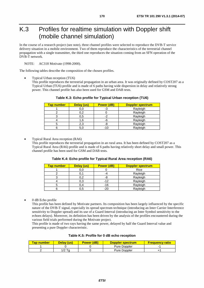
ETSI
ETSI TR 101 290 V1.3.1 (2014-07) 170
K.3 Profiles for realtime simulation with Doppler shift (mobile channel simulation)
In the course of a research project (see note), three channel profiles were selected to reproduce the DVB-T service delivery situation in a mobile environment. Two of them reproduce the characteristics of the terrestrial channel propagation with a single transmitter, the third one reproduces the situation coming from an SFN operation of the DVB-T network.
NOTE: AC318 Motivate (1998-2000).
The following tables describe the composition of the chosen profiles.
• Typical Urban reception (TU6) This profile reproduces the terrestrial propagation in an urban area. It was originally defined by COST207 as a Typical Urban (TU6) profile and is made of 6 paths having wide dispersion in delay and relatively strong power. This channel profile has also been used for GSM and DAB tests.
Table K.3: Echo profile for Typical Urban reception (TU6)
Tap number Delay (us) Power (dB) Doppler spectrum 1 0,0 -3 Rayleigh 2 0,2 0 Rayleigh 3 0,5 -2 Rayleigh 4 1,6 -6 Rayleigh 5 2,3 -8 Rayleigh 6 5,0 -10 Rayleigh
• Typical Rural Area reception (RA6) This profile reproduces the terrestrial propagation in an rural area. It has been defined by COST207 as a Typical Rural Area (RA6) profile and is made of 6 paths having relatively short delay and small power. This channel profile has been used for GSM and DAB tests.
Table K.4: Echo profile for Typical Rural Area reception (RA6)
Tap number Delay (us) Power (dB) Doppler spectrum 1 0,0 0 Rice 2 0,1 -4 Rayleigh 3 0,2 -8 Rayleigh 4 0,3 -12 Rayleigh 5 0,4 -16 Rayleigh 6 0,5 -20 Rayleigh
• 0 dB Echo profile This profile has been defined by Motivate partners. Its composition has been largely influenced by the specific nature of the DVB-T signal, especially its spread spectrum technique (introducing an Inter Carrier Interference sensitivity to Doppler spread) and its use of a Guard Interval (introducing an Inter Symbol sensitivity to the echoes delays). Moreover, its definition has been driven by the analysis of the profiles encountered during the various field trials performed during the Motivate project. This profile is made of two rays having the same power, delayed by half the Guard Interval value and presenting a pure Doppler characteristic.
Table K.5: Profile for 0 dB echo reception
Tap number Delay (us) Power (dB) Doppler spectrum Frequency ratio 1 0 0 Pure Doppler -1 2 1/2 Tg 0 Pure Doppler +1

ETSI
ETSI TR 101 290 V1.3.1 (2014-07) 171
Annex L: The measurement of MER under ACE When ACE method means Active Constellation Extension, it uses outer point constellation points of the useful carriers to reduce the Peak to Average value of the DVB-T2 signals. It is an option of the DVB-T2 standard and it is used for example in the L1 signalling parameters since EN 302 755 (V1.3.1) [i.27].
When ACE is applied on a COFDM signal, the professional receiver is not capable of referring to the theoretical reference point in order to measure the modulation error distance as in the formula.
The problem is to find a solution that allows MER measurement on carriers when Active Constellation Extension is used on a DVB-T2 signal.
1) Enable Active constellation point.
2) Disable ACE on some carriers based on a circular mask pattern. The number of useful carriers is less than 1% in order not to impact the Peak to Average Ratio of the final signal.
3) This method is a test mode located in the modulation part implementing ACE algorithm. The receiver can recover the MER based on the mask pattern definition.
The ACE method is defined in clause 9.6.1 of EN 302 755 [i.27].
Figure L.1: Implementation of the ACE method (extracted from EN 302 755 [i.27])
In the block diagram above, "extendable" signification is modified from the DVB-T2 specification EN 302 755 [i.27] clause 9.6.1, in order to add a circular mask pattern exclusion.
Standard definition of "extendable":
A component is defined as extendable if it is an active cell (i.e. an OFDM cell carrying a constellation point for L1 signalling or a PLP), and if its absolute amplitude is greater than or equal to the maximal component value associated to the modulation constellation used for that cell; a component is also defined as extendable if it is a dummy cell, a bias balancing cell or an unmodulated cell in the Frame Closing Symbol.

ETSI
ETSI TR 101 290 V1.3.1 (2014-07) 172
For the test mode, the text is adjusted:
A component is defined as extendable if it is an active cell (i.e. an OFDM cell carrying a constellation point for L1 signalling or a PLP), and if its absolute amplitude is greater than or equal to the maximal component value associated to the modulation constellation used for that cell; a component is also defined as extendable if it is a dummy cell, a bias balancing cell or an unmodulated cell in the Frame Closing Symbol. In test mode, active cells corresponding to the mask pattern index position list are not extended.
The circular mask pattern is changed for each new T2 frame symbol in order to measure MER for all the carriers.
The mask pattern M[] for ACE is defined as follows:
Idx=Frame Idx mod 100; i=0; While (idx<Cuseful) { Idx=mod(Idx+div(Cuseful /100), Cuseful) M[i]=idx; i++; }
For a given frame index, where Idx provides the carrier position and M[] is the mask pattern containing index position is ascendant form defined for a Frame number FrameIdx.
Where Cuseful
Cuseful = Cdata for data symbols
Cuseful= CP2 for P2 symbols
Cuseful = CFC for Frame closing symbols

ETSI
ETSI TR 101 290 V1.3.1 (2014-07) 173
Annex M: Bibliography
• ETSI TS 102 154: "Digital Video Broadcasting (DVB); Implementation guidelines for the use of Video and Audio Coding in Contribution and Primary Distribution Applications based on the MPEG-2 Transport Stream".
• Recommendation ITU-T G.826: "Error performance parameters and objectives for international, constant bit rate digital paths at or above the primary rate".
• ETSI TR 101 290 (V1.2.1) 2001-05: "Digital Video Broadcasting (DVB); Measurement guidelines for DVB systems".

ETSI
ETSI TR 101 290 V1.3.1 (2014-07) 174
History
Document history
Edition 1 May 1997 Publication as ETR 290
V1.2.1 May 2001 Publication
V1.3.1 July 2014 Publication
V1.3.1 July 2014 Publication
V1.3.1 July 2014 Publication


