TR 145 050 - V12.2.0 - Digital cellular telecommunications ... · A.2 SCENARIO 2 - MULTIPLE MS AND...

ETSI TR 1

Digital cellular telecoBackground for Ra

(3GPP TR 45.0

TECHNICAL REPORT

145 050 V12.2.0 (2015

communications system (PhaRadio Frequency (RF) requirem.050 version 12.2.0 Release 12

GLOBAL SYSTEMOBILE COMMUN

15-04)

hase 2+); rements 12)

TEM FOR UNICATIONS

R

ETSI

ETSI TR 145 050 V12.2.0 (2015-04)13GPP TR 45.050 version 12.2.0 Release 12

Reference RTR/TSGG-0145050vc20

Keywords GSM

ETSI

650 Route des Lucioles F-06921 Sophia Antipolis Cedex - FRANCE

Tel.: +33 4 92 94 42 00 Fax: +33 4 93 65 47 16

Siret N° 348 623 562 00017 - NAF 742 C

Association à but non lucratif enregistrée à la Sous-Préfecture de Grasse (06) N° 7803/88

Important notice

The present document can be downloaded from: http://www.etsi.org/standards-search

The present document may be made available in electronic versions and/or in print. The content of any electronic and/or print versions of the present document shall not be modified without the prior written authorization of ETSI. In case of any

existing or perceived difference in contents between such versions and/or in print, the only prevailing document is the print of the Portable Document Format (PDF) version kept on a specific network drive within ETSI Secretariat.

Users of the present document should be aware that the document may be subject to revision or change of status. Information on the current status of this and other ETSI documents is available at

http://portal.etsi.org/tb/status/status.asp

If you find errors in the present document, please send your comment to one of the following services: https://portal.etsi.org/People/CommiteeSupportStaff.aspx

Copyright Notification

No part may be reproduced or utilized in any form or by any means, electronic or mechanical, including photocopying and microfilm except as authorized by written permission of ETSI.

The content of the PDF version shall not be modified without the written authorization of ETSI. The copyright and the foregoing restriction extend to reproduction in all media.

© European Telecommunications Standards Institute 2015.

All rights reserved.

DECTTM, PLUGTESTSTM, UMTSTM and the ETSI logo are Trade Marks of ETSI registered for the benefit of its Members. 3GPPTM and LTE™ are Trade Marks of ETSI registered for the benefit of its Members and

of the 3GPP Organizational Partners. GSM® and the GSM logo are Trade Marks registered and owned by the GSM Association.

http://www.etsi.org/standards-search

http://portal.etsi.org/tb/status/status.asp

https://portal.etsi.org/People/CommiteeSupportStaff.aspx

ETSI


Intellectual Property Rights IPRs essential or potentially essential to the present document may have been declared to ETSI. The information pertaining to these essential IPRs, if any, is publicly available for ETSI members and non-members, and can be found in ETSI SR 000 314: "Intellectual Property Rights (IPRs); Essential, or potentially Essential, IPRs notified to ETSI in respect of ETSI standards", which is available from the ETSI Secretariat. Latest updates are available on the ETSI Web server (http://ipr.etsi.org).

Pursuant to the ETSI IPR Policy, no investigation, including IPR searches, has been carried out by ETSI. No guarantee can be given as to the existence of other IPRs not referenced in ETSI SR 000 314 (or the updates on the ETSI Web server) which are, or may be, or may become, essential to the present document.

Foreword This Technical Report (TR) has been produced by ETSI 3rd Generation Partnership Project (3GPP).

The present document may refer to technical specifications or reports using their 3GPP identities, UMTS identities or GSM identities. These should be interpreted as being references to the corresponding ETSI deliverables.

The cross reference between GSM, UMTS, 3GPP and ETSI identities can be found under http://webapp.etsi.org/key/queryform.asp.

Modal verbs terminology In the present document "shall", "shall not", "should", "should not", "may", "need not", "will", "will not", "can" and "cannot" are to be interpreted as described in clause 3.2 of the ETSI Drafting Rules (Verbal forms for the expression of provisions).

"must" and "must not" are NOT allowed in ETSI deliverables except when used in direct citation.

http://webapp.etsi.org/IPR/home.asp

http://webapp.etsi.org/key/queryform.asp

http://portal.etsi.org/Help/editHelp!/Howtostart/ETSIDraftingRules.aspx

ETSI


Contents

Intellectual Property Rights ................................................................................................................................ 2

Foreword ............................................................................................................................................................. 2

Modal verbs terminology .................................................................................................................................... 2

Foreword ........................................................................................................................................................... 19

1 Scope ...................................................................................................................................................... 20

2 Information available ............................................................................................................................. 20

3 DCS1800 system scenarios .................................................................................................................... 20

4 GSM900 small cell system scenarios ..................................................................................................... 21

5 GSM900 and DCS1800 microcell system scenarios .............................................................................. 21

6 Conversion factors .................................................................................................................................. 22

7 Repeaters ................................................................................................................................................ 22

8 Error Patterns for Speech Coder Developments ..................................................................................... 23

9 Simulations of Performance ................................................................................................................... 23

10 GSM900 railway system scenarios ........................................................................................................ 23

11 Simulation results for GPRS receiver performance ............................................................................... 24

12 Pico BTS RF scenarios ........................................................................................................................... 24

13 CTS system scenarios ............................................................................................................................. 24

14 GSM400 system scenarios ..................................................................................................................... 24

15 MXM system scenarios .......................................................................................................................... 24

16 LCS scenarios ......................................................................................................................................... 24

17 8-PSK Scenarios ..................................................................................................................................... 24

18 T-GSM 900 System Scenarios ............................................................................................................... 24

19 MBMS System Scenarios ....................................................................................................................... 24

20 T-GSM 810 System Scenarios ............................................................................................................... 25

21 Multicarrier BTS Class ........................................................................................................................... 25

22 ER-GSM band introduction.................................................................................................................... 25

23 Extended Training Sequence Code Sets ................................................................................................. 25

23.1 Background ...................................................................................................................................................... 25

23.2 Extended TSC Sets ........................................................................................................................................... 25

23.2.1 Scope .......................................................................................................................................................... 25

23.2.2 Design criteria ............................................................................................................................................. 26

23.2.3 Design methodology ................................................................................................................................... 26

23.2.4 Evaluation methodology ............................................................................................................................. 26

23.2.5 Performance evaluation .............................................................................................................................. 26

Annex A: DCS1800 System scenarios................................................................................................... 27

A.0 INTRODUCTION .................................................................................................................................. 27

A.1 SCENARIO 1 - SINGLE BTS AND MS ............................................................................................... 27

A.1.1 Constraints ........................................................................................................................................................ 27

A.1.1.1 Frequency Bands and Channel Arrangement (Clause 2 of GSM 05.05) .................................................... 27

ETSI


A.1.1.2 Proximity .................................................................................................................................................... 28

A.1.1.3 Range .......................................................................................................................................................... 28

A.1.3 Inputs needed .................................................................................................................................................... 29

A.2 SCENARIO 2 - MULTIPLE MS AND BTS, COORDINATED .......................................................... 29

A.2.1 Constraints ........................................................................................................................................................ 29

A.2.3 Inputs needed .................................................................................................................................................... 30

A.3 SCENARIO 3 - MULTIPLE MS AND BTS, UNCOORDINATED ..................................................... 31

A.3.1 Constraints ........................................................................................................................................................ 31

A.3.3 Inputs needed .................................................................................................................................................... 31

A.4 SCENARIO 4 - COLOCATED MS ....................................................................................................... 32

A.4.1 Constraints ........................................................................................................................................................ 32

A.4.3 Inputs needed .................................................................................................................................................... 33

A.5 SCENARIO 5 - COLOCATED BTS ..................................................................................................... 33

A.5.1 Constraints ........................................................................................................................................................ 33

A.5.3 Inputs needed .................................................................................................................................................... 33

A.6 SCENARIO 6 - COLOCATION WITH OTHER SYSTEMS ............................................................... 34

A.6.1 Constraints ........................................................................................................................................................ 34

A.6.3 Inputs needed .................................................................................................................................................... 34

A.7 Title: Justifications for the proposed Rec. 05.05_DCS .......................................................................... 35

A.7.1 Transmitter ....................................................................................................................................................... 36

A.7.1.1 Modulation, Spurs and Noise ...................................................................................................................... 36

A.7.1.1.1 Co-ordinated, BTS -> MS (Scenario 2, figure 2.1) ............................................................................... 36

A.7.1.1.2 Uncoordinated, BTS -> MS (Scenario 3, figure 3.1) ............................................................................ 36

A.7.1.1.3 Co-ordinated & Uncoordinated MS -> BTS (Scenarios 2 and 3, figures 2.1 and 3.1) ................................ 36

A.7.1.1.4 Co-ordinated & Uncoordinated MS->MS (Scenario 4) ........................................................................ 36

A.7.1.1.5 Co-ordinated & Uncoordinated BTS->BTS (Scenario 5) ..................................................................... 36

A.7.1.2 Switching Transients................................................................................................................................... 36

A.7.1.2.1 Uncoordinated MS -> BTS (Scenario 3, figure 3.1) ............................................................................. 36

A.7.1.2.2 Uncoordinated BTS -> MS (Scenario 3, figure 3.1) ............................................................................. 36

A.7.1.3 Intermodulation ........................................................................................................................................... 37

A.7.1.3.1 Co-ordinated, BTS -> MS (Scenario 2, figures 2.2 and 2.3) ................................................................. 37

A.7.1.3.2 Uncoordinated, BTS ->MS (Scenario 3, figure 3.2 top) ....................................................................... 37

A.7.1.3.3 Uncoordinated, MS&MS-> BTS (Scenario 4, figure 4.1 bottom) ........................................................ 37

A.7.1.3.4 Uncoordinated MS&MS-> MS (Scenario 4, figure 4.1 top) ................................................................. 37

A.7.2 Receiver ............................................................................................................................................................ 37

A.7.2.1 Blocking ...................................................................................................................................................... 37

A.7.2.1.1 Co-ordinated & Uncoordinated BTS-> MS (Scenarios 2 and 3, figures 2.1 and 3.1) ................................. 37

A.7.2.1.2 Co-ordinated MS-> BTS (Scenario 2, figure 2.1) ................................................................................. 37

A.7.2.1.3 Uncoordinated MS-> BTS (Scenario 3, figure 3.1) .............................................................................. 37

A.7.2.1.4 Co-ordinated & Uncoordinated MS-> MS (Scenario 4) ....................................................................... 37

A.7.2.1.5 Co-ordinated & Uncoordinated BTS-> BTS (Scenario 5) .................................................................... 37

A.7.2.2 Intermodulation ........................................................................................................................................... 38

A.7.2.2.1 Co-ordinated & Uncoordinated BTS-> MS (Scenarios 2 and 3, figure 3.2 middle) ............................. 38

A.7.2.2.2 Co-ordinated MS & MS -> BTS (Scenario 4) ....................................................................................... 38

A.7.2.2.3 Uncoordinated MS & MS -> BTS (Scenario 4, figure 3.2 lower) ......................................................... 38

A.7.2.3 Maximum level ........................................................................................................................................... 38

A.7.2.3.1 Co-ordinated MS -> BTS (Scenario 1).................................................................................................. 38

A.7.2.3.2 Co-ordinated BTS -> MS (Scenario 1).................................................................................................. 38

A.8.1 SCOPE ............................................................................................................................................................. 38

A.8.2 FREQUENCY BANDS AND CHANNEL ARRANGEMENT ...................................................................... 38

A.8.3 REFERENCE CONFIGURATION ................................................................................................................. 38

A.8.4 TRANSMITTER CHARACTERISTICS ......................................................................................................... 39

A.8.4.1 Output power .............................................................................................................................................. 39

A.8.4.1.1 Mobile Station ....................................................................................................................................... 39

A.8.4.1.2 Base Station........................................................................................................................................... 39

A.8.4.2 Output RF spectrum .................................................................................................................................... 39

A.8.4.2.1 Spectrum due to the modulation ............................................................................................................ 39

A.8.4.2.2 Spectrum due to switching transients .................................................................................................... 40

ETSI


A.8.4.3 Spurious emissions ..................................................................................................................................... 40

A.8.4.3.1 Principle of the specification ................................................................................................................. 40

A.8.4.3.2 Base Station........................................................................................................................................... 40

A.8.4.3.3 Mobile Station ....................................................................................................................................... 40

A.8.4.4 Radio frequency tolerance .......................................................................................................................... 41

A.8.4.5 Output level dynamic operation .................................................................................................................. 41

A.8.4.5.1 Base station ........................................................................................................................................... 41

A.8.4.5.2 Mobile station: ...................................................................................................................................... 41

A.8.4.6 Phase accuracy ............................................................................................................................................ 41

A.8.4.7 Intermodulation attenuation ........................................................................................................................ 41

A.8.4.7.1 Base transceiver station ......................................................................................................................... 41

A.8.4.7.2 Intra BTS intermodulation attenuation .................................................................................................. 41

A.8.4.7.3 Intermodulation between MS ................................................................................................................ 41

A.8.5 RECEIVER CHARACTERISTICS ................................................................................................................. 42

A.8.5.1 Blocking characteristics .............................................................................................................................. 42

A.8.5.2 Intermodulation characteristics ................................................................................................................... 43

A.8.5.3 Spurious response rejection ........................................................................................................................ 43

A.8.5.4 Spurious emissions ..................................................................................................................................... 43

A.8.6 TRANSMITTER/RECEIVER PERFORMANCE ........................................................................................... 43

A.8.6.1 Nominal error rates (NER) ......................................................................................................................... 43

A.8.6.2 Reference sensitivity level .......................................................................................................................... 43

A.8.6.3 Reference interference level ....................................................................................................................... 44

A.8.6.4 Erroneous frame indication performance .................................................................................................... 44

Annex B: GSM900 Small Cell System scenarios ................................................................................. 45

B.1 Transmitter ............................................................................................................................................. 46

B.1.1 Modulation, Spurs and Noise ........................................................................................................................... 46

B.1.1.1 Co-ordinated, BTS -> MS ........................................................................................................................... 46

B.1.1.2 Uncoordinated, BTS -> MS ........................................................................................................................ 46

B.1.1.3 Co-ordinated & Uncoordinated MS -> BTS ............................................................................................... 46

B.1.1.4 Co-ordinated & Uncoordinated MS -> MS................................................................................................. 46

B.1.1.5 Co-ordinated & Uncoordinated BTS -> BTS ............................................................................................. 47

B.1.2 Switching Transients ........................................................................................................................................ 47

B.1.2.1 Uncoordinated MS -> BTS ......................................................................................................................... 47

B.1.2.2 Uncoordinated BTS -> MS ......................................................................................................................... 47

B.1.3 Intermodulation ................................................................................................................................................ 47

B.1.3.1 Coordinated, BTS -> MS ............................................................................................................................ 47

B.1.3.2 Uncoordinated, BTS -> MS ........................................................................................................................ 47

B.1.3.3 Uncoordinated, MS&MS -> BTS ............................................................................................................... 47

B.1.3.4 Uncoordinated MS&MS -> MS .................................................................................................................. 47

B.2 Receiver .................................................................................................................................................. 47

B.2.1 Blocking ........................................................................................................................................................... 47

B.2.1.1 Co-ordinated & Uncoordinated BTS -> MS ............................................................................................... 47

B.2.1.2 Co-ordinated MS -> BTS ............................................................................................................................ 47

B.2.1.3 Uncoordinated MS -> BTS ......................................................................................................................... 48

B.2.1.4 Co-ordinated & Uncoordinated MS -> MS................................................................................................. 48

B.2.1.5 Co-ordinated and Uncoordinated BTS -> BTS ........................................................................................... 48

B.2.2 Intermodulation ................................................................................................................................................ 48

B.2.2.1 Co-ordinated & Uncoordinated BTS -> MS ............................................................................................... 48

B.2.2.2 Co-ordinated MS & MS -> BTS ................................................................................................................. 48

B.2.2.3 Uncoordinated MS & MS -> BTS .............................................................................................................. 48

B.2.3 Maximum level ................................................................................................................................................ 48

B.2.3.1 Co-ordinated MS -> BTS ............................................................................................................................ 48

B.2.3.2 Co-ordinated BTS -> MS ............................................................................................................................ 48

B.3.1 Transmitter ....................................................................................................................................................... 49

B.3.1.1 Modulation, Spurs and Noise ...................................................................................................................... 49

B.3.1.1.1 Co-ordinated, BTS -> MS ..................................................................................................................... 49

B.3.1.1.2 Uncoordinated, BTS -> MS .................................................................................................................. 49

B.3.1.1.3 Co-ordinated & Uncoordinated MS -> BTS ......................................................................................... 49

B.3.1.1.4 Co-ordinated & Uncoordinated MS -> MS ........................................................................................... 49

B.3.1.1.5 Co-ordinated & Uncoordinated BTS -> BTS ........................................................................................ 49

ETSI


B.3.1.2 Switching Transients................................................................................................................................... 49

B.3.1.2.1 Uncoordinated MS -> BTS ................................................................................................................... 49

B.3.1.2.2 Uncoordinated BTS -> MS ................................................................................................................... 49

B.3.1.3 Intermodulation ........................................................................................................................................... 50

B.3.1.3.1 Coordinated, BTS -> MS ...................................................................................................................... 50

B.3.1.3.2 Uncoordinated, BTS -> MS .................................................................................................................. 50

B.3.1.3.3 Uncoordinated, MS&MS -> BTS.......................................................................................................... 50

B.3.1.3.4 Uncoordinated MS&MS -> MS ............................................................................................................ 50

B.3.2 Receiver ............................................................................................................................................................ 50

B.3.2.1 Blocking ...................................................................................................................................................... 50

B.3.2.1.1 Co-ordinated & Uncoordinated BTS -> MS ......................................................................................... 50

B.3.2.1.2 Co-ordinated MS -> BTS ...................................................................................................................... 50

B.3.2.1.3 Uncoordinated MS -> BTS ................................................................................................................... 50

B.3.2.1.4 Co-ordinated & Uncoordinated MS -> MS ........................................................................................... 50

B.3.2.1.5 Co-ordinated and Uncoordinated BTS -> BTS ..................................................................................... 50

B.3.2.2 Intermodulation ........................................................................................................................................... 50

B.3.2.2.1 Co-ordinated & Uncoordinated BTS -> MS ......................................................................................... 50

B.3.2.2.2 Co-ordinated MS & MS -> BTS ........................................................................................................... 51

B.3.2.2.3 Uncoordinated MS & MS -> BTS......................................................................................................... 51

B.3.2.3 Maximum level ........................................................................................................................................... 51

B.3.2.3.1 Co-ordinated MS -> BTS ...................................................................................................................... 51

B.3.2.3.2 Co-ordinated BTS -> MS ...................................................................................................................... 51

Annex C: Microcell System Scenarios .................................................................................................. 52

Annex D: Conversion factors ................................................................................................................ 65

Annex E: Repeater Scenarios................................................................................................................ 69

E.1 INTRODUCTION .................................................................................................................................. 69

E.2 REPEATER APPLICATIONS - OUTDOOR AND INDOOR ............................................................. 69

E.3 OUTDOOR REPEATER SCENARIO .................................................................................................. 69

E.4 OUTDOOR REPEATER PERFORMANCE Requirements .................................................................. 70

E.4.1 Wideband Noise ............................................................................................................................................... 70

E.4.2 Intermodulation Products and Spurious Emissions .......................................................................................... 71

E.4.3 Output Power .................................................................................................................................................... 71

E.4.4 Blocking by Uncoordinated BTS ..................................................................................................................... 71

E.4.5 Summary of Outdoor Repeater Requirements .................................................................................................. 72

E.5 INDOOR REPEATER SCENARIO ...................................................................................................... 72

E.6 INDOOR REPEATER PERFORMANCE REQUIREMENTS ............................................................. 72

E.6.1 Wideband Noise ............................................................................................................................................... 72

E.6.2 Intermodulation Products and Spurious Emissions .......................................................................................... 73

E.6.3 Output Power .................................................................................................................................................... 73

E.6.4 Blocking by Uncoordinated BTS ..................................................................................................................... 74

E.6.5 Summary of Indoor Repeater Requirements .................................................................................................... 74

E.7 Title: Repeater Scenarios........................................................................................................................ 75

E.7.1 Introduction ...................................................................................................................................................... 75

E.7.2 Repeater performance ....................................................................................................................................... 75

E.7.2.1 Link Equations ............................................................................................................................................ 75

E.7.2.2 Co-ordinated Scenario ................................................................................................................................ 76

E.7.2.3 Uncoordinated Scenario .............................................................................................................................. 77

E.7.2.4 Wideband Noise .......................................................................................................................................... 77

E.7.2.5 3rd order Intermodulation (IM3) performance/Spurious emissions: .......................................................... 77

E.7.3 Repeater scenarios ............................................................................................................................................ 77

E.7.3.1 Rural scenario ............................................................................................................................................. 78

E.7.3.2 Urban Scenario ........................................................................................................................................... 78

E.7.4 Summary .......................................................................................................................................................... 79

E.7.4.1 Repeater Specification ................................................................................................................................ 79

E.7.4.2 Planning considerations .............................................................................................................................. 79

ETSI


E.7.5 Out of band Gain .............................................................................................................................................. 80

E.7.6 Planning guidelines for repeaters ................................................................................................................ 80

E.7.7 Indoor Repeater Scenario ................................................................................................................................. 80

Annex F: Error Patterns for Speech Coder Development ................................................................. 84

F.0 Introduction ............................................................................................................................................ 84

F.1 Channel Conditions ................................................................................................................................ 84

F.1.1 Simulation Conditions ...................................................................................................................................... 84

F.1.2 Available Error Patterns ................................................................................................................................... 84

F.2 Test Data for the half rate speech coder ................................................................................................. 85

F.2.1 File description ................................................................................................................................................. 85

F.2.2 Soft decision values and chip error patterns ..................................................................................................... 85

F.2.3 Error patterns of corresponding TCH/FS ......................................................................................................... 86

Annex G: Simulation of Performance .................................................................................................. 88

G.1 Implementation Losses and Noise Figure .............................................................................................. 88

G.1.1 Assumed Equalizer ........................................................................................................................................... 88

G.1.2 Accuracy of Simulations .................................................................................................................................. 88

G.1.3 Simulation Results ............................................................................................................................................ 88

G.2 Reference Structure ................................................................................................................................ 97

G.2.1 Error Concealment ........................................................................................................................................... 98

G.2.2 Implementation Losses and Noise Figure ........................................................................................................ 98

G.2.3 Assumed Equalizer ........................................................................................................................................... 98

G.2.4 Simulation Results ............................................................................................................................................ 98

G.2.5 Proposed Values for Recommendation GSM 05.05 ......................................................................................... 98

G.3 Simulation of performance for AMR ..................................................................................................... 99

G.3.1 System Configuration ....................................................................................................................................... 99

G.3.2 Error Concealment ........................................................................................................................................... 99

G.3.3 Implementation Losses and Noise Figure ...................................................................................................... 100

G.3.4 Assumed Equalizer ......................................................................................................................................... 100

G.3.5 Simulation Methods ....................................................................................................................................... 100

G.3.5.1 Simulation for speech ............................................................................................................................... 100

G.3.5.2 Simulation for DTX .................................................................................................................................. 100

G.3.5.3 Simulation for inband channel .................................................................................................................. 100

G.3.6 Remarks to the Data in GSM 05.05 ................................................................................................................ 101

Annex H: GSM900 Railway System Scenarios .................................................................................. 102

H.1 Scope .................................................................................................................................................... 102

H.1.1 List of some abbreviations.............................................................................................................................. 102

H.2 Constraints ............................................................................................................................................ 102

H.2.1 GSM based systems in the 900 MHz band ..................................................................................................... 102

H.2.2 Other systems ................................................................................................................................................. 103

H.2.3 UIC systems outline ....................................................................................................................................... 103

H.2.4 Fixed UIC RF parameters ............................................................................................................................... 103

H.3 Methodology ........................................................................................................................................ 103

H.3.1 Scenarios ........................................................................................................................................................ 104

H.3.2 Format of calculations .................................................................................................................................... 105

H.3.3 GSM900 systems parameters ......................................................................................................................... 105

H.3.4 Minimum Coupling Loss ................................................................................................................................ 106

H.3.5 Interference margins ....................................................................................................................................... 107

H.3.6 Differences between E- and P-GSM .............................................................................................................. 107

H4 Transmitter requirements ..................................................................................................................... 107

H.4.1 Transmitter requirements summary ................................................................................................................ 108

H.5 Receiver requirements .......................................................................................................................... 108

H.5.1 Receiver requirements summary .................................................................................................................... 109

ETSI


H.6 Wanted signals levels ........................................................................................................................... 109

H.6.1 Maximum wanted signal level ........................................................................................................................ 110

H.6.2 Dynamic range of wanted signals ................................................................................................................... 110

Annex I: Void ...................................................................................................................................... 111

Annex J: GSM900 Railway System Scenarios .................................................................................. 112

J.1 Introduction .......................................................................................................................................... 112

J.2 Basic considerations ............................................................................................................................. 112

J.2.1 Types of equipment and frequency ranges ..................................................................................................... 112

J.3 Discussion of the individual sections in GSM 05.05 ........................................................................... 113

J.3.1 Scope .............................................................................................................................................................. 113

J.3.2 Frequency bands and channel arrangement .................................................................................................... 113

J.3.3 Reference configuration ................................................................................................................................. 114

J.3.4 Transmitter characteristics.............................................................................................................................. 114

J.3.4.1 Output power ............................................................................................................................................ 114

J.3.4.2 Void .......................................................................................................................................................... 114

J.3.4.2.1 Spectrum due to the modulation and wide band noise ........................................................................ 114

J.3.4.2.2a MS spectrum due to switching transients ............................................................................................ 114

J.3.4.2.2b BTS spectrum due to switching transients .......................................................................................... 115

J.3.4.3.1 Spurious emissions .............................................................................................................................. 115

J.3.4.3.2 BTS spurious emissions ...................................................................................................................... 116

J.3.4.3.3 MS spurious emissions ........................................................................................................................ 116

J.3.4.3.4 MS spurious emissions onto downlinks .............................................................................................. 117

J.3.4.4 Radio frequency tolerance ........................................................................................................................ 118

J.3.4.5 Output level dynamic operation ................................................................................................................ 118

J.3.4.5.1 BTS output level dynamic operation ................................................................................................... 118

J.3.4.5.2 MS output level dynamic operation .................................................................................................... 119

J.3.4.6 Phase accuracy .......................................................................................................................................... 119

J.3.4.7.1 Intra BTS intermod attenuation ........................................................................................................... 119

J.3.4.7.2 Intermodulation between MS (DCS1800 only) ................................................................................... 119

J.3.4.7.3 Mobile PBX ........................................................................................................................................ 119

J.3.5 Receiver characteristics .................................................................................................................................. 120

J.3.5.1 Blocking characteristics ............................................................................................................................ 120

J.3.5.2 Blocking characteristics (in-band) ............................................................................................................ 120

J.3.5.3 Blocking characteristics (out-of-band)...................................................................................................... 121

J.3.5.4 AM suppresion characteristics .................................................................................................................. 121

J.3.5.5 Intermodulation characteristics ................................................................................................................. 121

J.3.5.6 Spurious emissions ................................................................................................................................... 121

J.3.6 Transmitter/receiver performance .................................................................................................................. 121

J.3.6.1 Nominal error rates ................................................................................................................................... 121

J.3.6.2 Reference sensitivity level ........................................................................................................................ 121

Annex K: Block Erasure Rate Performance for GPRS .................................................................... 123

K.1 Introduction .......................................................................................................................................... 123

K.2 Simulation Model ................................................................................................................................. 123

K.3 Results .................................................................................................................................................. 123

K.4 Conclusions .......................................................................................................................................... 124

Annex L: Proposal on how to report GPRS performance into GSM 05.05 .................................... 125

L.1 Introduction .......................................................................................................................................... 125

L.2 GPRS BLER performance.................................................................................................................... 125

L.3 GPRS throughput analyses ................................................................................................................... 126

L.3.1 TU50 ideal FH ................................................................................................................................................ 127

L.3.2 TU3 no FH ..................................................................................................................................................... 128

ETSI


L.4 Proposals for GPRS performance in GSM 05.05 ................................................................................. 128

L.4.1 TU50 ideal FH ................................................................................................................................................ 128

L.4.2 TU3 no FH ..................................................................................................................................................... 129

L.5 Conclusions .......................................................................................................................................... 129

Annex M: GPRS simulation results in TU 3 and TU 50 no FH ........................................................ 130

M.1 Introduction .......................................................................................................................................... 130

M.2 Simulation Model ................................................................................................................................. 130

M.3 Maximum GPRS throughput ................................................................................................................ 132

M.4 Conclusion ............................................................................................................................................ 133

M.5 References ............................................................................................................................................ 133

Annex N: C/Ic and Eb/No Radio Performance for the GPRS Coding Schemes ............................... 134

N.1 Introduction .......................................................................................................................................... 134

N.2 C/I simulation results............................................................................................................................ 134

N.3 Eb/N0 performance ................................................................................................................................ 136

N.4 Conclusions .......................................................................................................................................... 138

N.5 References ............................................................................................................................................ 138

Annex O: Void ...................................................................................................................................... 139

Annex P: Block Error Rate and USF Error Rate for GPRS ........................................................... 140

P.1 Introduction .......................................................................................................................................... 140

P.2 Simulation Assumptions....................................................................................................................... 140

P.3 Simulation Results ................................................................................................................................ 141

P.3.1 Interference Simulations ................................................................................................................................. 141

P.3.1.1 TU50 Ideal Frequency Hopping ............................................................................................................... 141

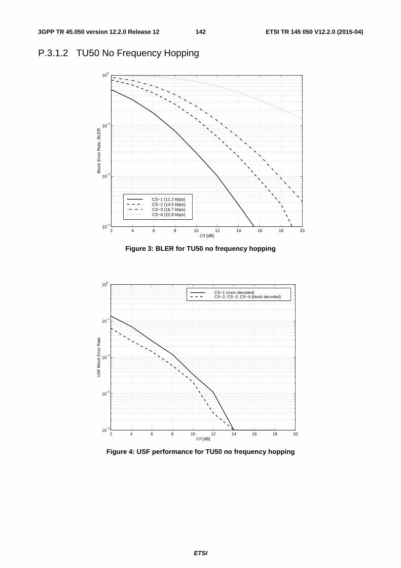
P.3.1.2 TU50 No Frequency Hopping .................................................................................................................. 142

P.3.1.3 TU3 Ideal Frequency Hopping ................................................................................................................. 143

P.3.1.4 TU3 No Frequency Hopping .................................................................................................................... 144

P.3.1.5 RA250 No Frequency Hopping ................................................................................................................ 145

P.3.2 Sensitivity Simulations ................................................................................................................................... 146

P.3.2.1 TU50 Ideal Frequency Hopping ............................................................................................................... 146

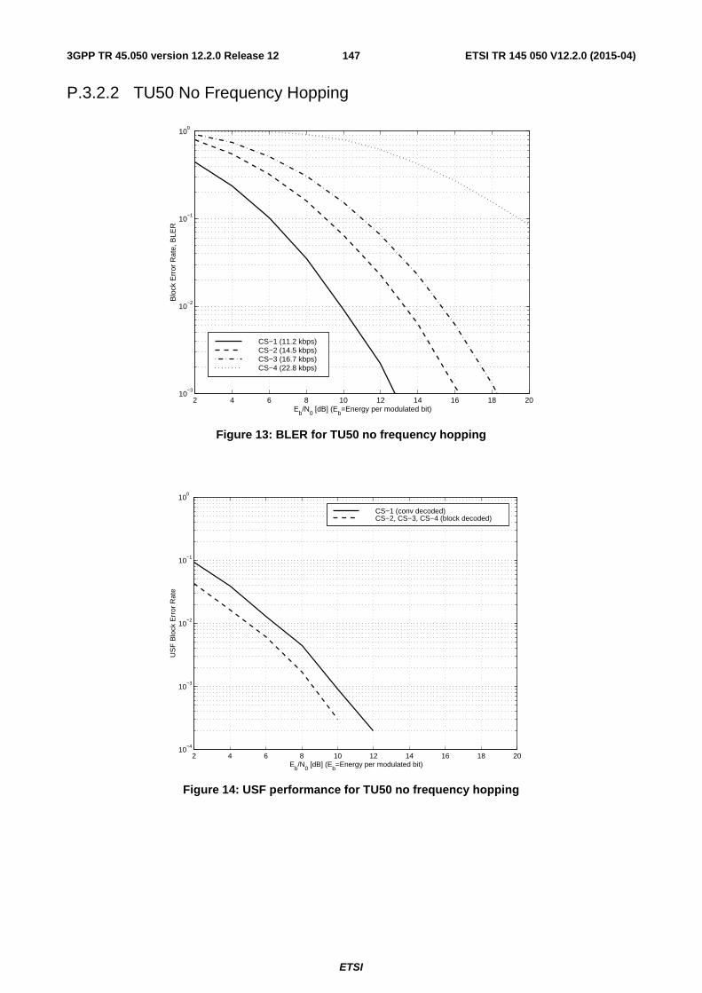
P.3.2.2 TU50 No Frequency Hopping .................................................................................................................. 147

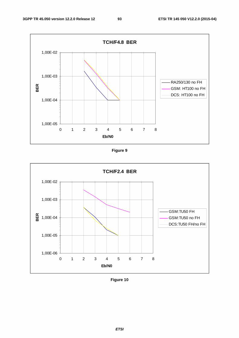
P.3.2.3 HT100 No Frequency Hopping ................................................................................................................ 148

P.3.2.4 RA250 No Frequency Hopping ................................................................................................................ 149

P.3.2.5 Static Channel ........................................................................................................................................... 150

Annex Q: Block Error Rate and USF Error Rate for GPRS, 1800 MHz ........................................ 151

Q.1 Introduction .......................................................................................................................................... 151

Q.2 Simulation Assumptions....................................................................................................................... 151

Q.3 Simulation Results ................................................................................................................................ 152

Q.3.1 Interference Simulations, 1 800 MHz............................................................................................................. 152

Q.3.1.2 TU50, Ideal Frequency Hopping .............................................................................................................. 152

Q.3.1.3 TU50 No Frequency Hopping .................................................................................................................. 153

Q.3.2 Sensitivity Simulations, 1800 MHz ................................................................................................................ 154

Q.3.2.1 TU50 Ideal Frequency Hopping ............................................................................................................... 154

Q.3.2.2 TU50 No Frequency Hopping .................................................................................................................. 155

Q.3.2.3 HT100 No Frequency Hopping ................................................................................................................ 156

Annex R: Pico BTS RF Scenarios ....................................................................................................... 157

ETSI


R.1 Introduction .......................................................................................................................................... 157

R.2 Fixed parameters .................................................................................................................................. 157

R.3 Maximum BTS Output Power .............................................................................................................. 158

R.4 BTS Receiver Sensitivity ..................................................................................................................... 159

R.4.1 Balanced link (zero interference scenario) ..................................................................................................... 159

R.4.2 Interferer at MCL scenario ............................................................................................................................. 159

R.4.3 Power control (zero interference scenario) ..................................................................................................... 160

R.4.4 Sensitivity overview ....................................................................................................................................... 160

R.5 BTS Power Control Range ................................................................................................................... 160

R.6 BTS Spectrum due to modulation and wideband noise ........................................................................ 160

R.7 Spurious Emissions .............................................................................................................................. 161

R.8 Radio Frequency Tolerance .................................................................................................................. 161

R.9 Blocking Characteristics....................................................................................................................... 162

R.10 pico- BTS AM suppression characteristics .......................................................................................... 163

R.10.1 Modulation sidebands ..................................................................................................................................... 164

R.10.1.1 Uncoordinated BTS->MS ......................................................................................................................... 164

R.10.1.2 Uncoordinated MS->BTS ......................................................................................................................... 164

R.10.2 Switching transients ....................................................................................................................................... 164



R.10.3 Blocking ......................................................................................................................................................... 165



R.10.4 The AM suppression requirement .................................................................................................................. 165

R.10.4.1 Downlink, BTS->MS ................................................................................................................................ 165

R.10.4.2 Uplink, MS->BTS ..................................................................................................................................... 165

R.10.4.3 Interference levels ..................................................................................................................................... 166

R.11 intermodulation .................................................................................................................................... 166

R.11.1 co-ordinated and uncoordinated BTS -> MS (scenarios 2 & 3, figure 3.2 middle) ........................................ 166

R.11.2 coordinated MS&MS -> BTS (scenario 4) ..................................................................................................... 166

R.11.3 uncoordinated MS&MS -> BTS (scenario 4, figure 3.2 lower) ..................................................................... 166

R.11.4 MCL relaxation .............................................................................................................................................. 167

R.12 Pico BTS TI1.5 performance requirements .......................................................................................... 167

R.12.1 Nominal Error Rates for Pico-BTS ................................................................................................................ 167

R.13 timing and synchronisation .................................................................................................................. 168

R.13.1 Steady state timing advance error ................................................................................................................... 168

R.13.2 Conventional BTS .......................................................................................................................................... 169

R.13.3 Pico-BTS ........................................................................................................................................................ 169

R.13.3.1 Pico-BTS relaxation .................................................................................................................................. 169

R.13.3.2 MS impact of Pico-BTS relaxation ........................................................................................................... 169

Annex S: CTS system scenarios ......................................................................................................... 171

S.1 Introduction .......................................................................................................................................... 171

S.1.1 Parameter Set .................................................................................................................................................. 171

S.1.1.1 Transmitter Parameter ............................................................................................................................... 171

S.1.1.2 Receiver Parameter ................................................................................................................................... 172

S.1.1.3 Minimum coupling loss values ................................................................................................................. 172

S.1.1.4 Path loss models ....................................................................................................................................... 172

S.1.1.5 Margins ..................................................................................................................................................... 173

S.2 Transmitter characteristics ................................................................................................................... 173

S.2.1 Maximum CTS-FP Transmit Power limited by MS blocking ........................................................................ 173

S.2.2 Maximum CTS-FP Transmit Power limited by Spectrum due to Modulation and WBN .............................. 174

ETSI


S.2.3 Specification of max. CTS-FP Transmit Power and CTS-FP Spectrum due to modulation and wide band noise ............................................................................................................................................................... 175

S.2.3.1 Maximum CTS-FP transmit power ........................................................................................................... 175

S.2.3.2 Spectrum due to modulation and wide band noise.................................................................................... 176

S.2.4 Balanced link for zero interference scenario (Interferer at MCL scenario) .................................................... 177

S.2.5 Range of Coverage for CTS: .......................................................................................................................... 177

S.2.6 Minimum CTS-FP transmit power ................................................................................................................. 178

S.2.7 Power Level Distribution ............................................................................................................................... 179

S.2.8 Spurious Emission .......................................................................................................................................... 179

S.3 Receiver characteristics ........................................................................................................................ 180

S.3.1 Blocking ......................................................................................................................................................... 180

S.3.2 AM suppression .............................................................................................................................................. 181

S.3.2.1 Spectrum due to modulation ..................................................................................................................... 181

S.3.2.2 Switching transients .................................................................................................................................. 182

S.3.2.3 Blocking .................................................................................................................................................... 183

S.3.2.4 Specification of AM Suppression ............................................................................................................. 183

S.3.3 Intermodulation .............................................................................................................................................. 184

S.3.3.1 uncoordinated CTS-MSs -> GSM-BTS .................................................................................................... 184

S.3.3.2 uncoordinated CTS-FPs -> MS ................................................................................................................. 184

S.3.3.3 uncoordinated GSM-MSs -> CTS-FP ....................................................................................................... 185

S.4 CTS-FP TI5 performance requirements ............................................................................................... 185

S.4.1 Nominal Error Rates for the CTS-FP ............................................................................................................. 185

S.5 Conclusion ............................................................................................................................................ 186

Annex T: GSM400 system scenarios .................................................................................................. 187

T.0 Introduction .......................................................................................................................................... 187

T.1 Frequency bands and channel arrangement .......................................................................................... 187

T.2 System Scenario Calculations for GSM400 systems ........................................................................... 188

T.2.1 Worst case proximity scenarios ...................................................................................................................... 188

T.3 Worst Case Scenario Requirements ..................................................................................................... 190

T.3.1 Transmitter ..................................................................................................................................................... 190

T.3.1.1 Modulation, Spurs and noise..................................................................................................................... 190

T.3.1.1.1 Co-ordinated BTS -> MS .................................................................................................................... 190

T.3.1.1.2 Uncoordinated BTS -> MS ................................................................................................................. 190

T.3.1.1.3 Coordinated & Uncoordinated MS -> BTS ......................................................................................... 190

T.3.1.1.4 Coordinated & Uncoordinated MS -> MS .......................................................................................... 190

T.3.1.1.5 Coordinated & Uncoordinated BTS -> BTS ...................................................................................... 190

T.3.1.2 Switching transients .................................................................................................................................. 190

T.3.1.2.1 Uncoordinated MS -> BTS ................................................................................................................. 190


T.3.1.3 Intermodulation ......................................................................................................................................... 191

T.3.1.3.1 Coordinated BTS -> MS ..................................................................................................................... 191


T.3.1.3.3 Uncoordinated MSs -> BTS ................................................................................................................ 191

T.3.1.3.4 Uncoordinated MS & MS -> MS ........................................................................................................ 191

T.3.2 Receiver .......................................................................................................................................................... 191

T.3.2.1 Blocking .................................................................................................................................................... 191

T.3.2.1.1 Coordinated & Uncoordinated BTS -> MS ........................................................................................ 191

T.3.2.1.2 Coordinated MS -> BTS ..................................................................................................................... 191


T.3.2.1.4 Coordinated & Uncoordinated MS -> MS ......................................................................................... 191

T.3.2.1.5 Coordinated & Uncoordinated BTS -> BTS ...................................................................................... 191

T.3.2.2 Intermodulation ......................................................................................................................................... 191

T.3.2.2.1 Coordinated & Uncoordinated BTS -> MS ........................................................................................ 191



T.3.2.3 Maximum level ......................................................................................................................................... 192

ETSI



T.3.2.3.2 Coordinated BTS -> MS .................................................................................................................... 192

T.4 Transmitter characteristics ................................................................................................................... 192

T.4.1 Output power .................................................................................................................................................. 192

T.4.1.1 Mobile Station .......................................................................................................................................... 192

T.4.1.2 Base Station .............................................................................................................................................. 192

T.4.2 Output RF Spectrum ....................................................................................................................................... 192

T.4.2.1 Spectrum due to the modulation and wideband noise ............................................................................... 192

T.4.2.2 Spectrum due to switching transients ....................................................................................................... 193

T.4.3 Spurious emissions ......................................................................................................................................... 193

T.4.3.1 Principle of the specification .................................................................................................................... 193

T.4.3.2 Base transceiver station ............................................................................................................................ 194

T.4.3.3 Mobile station ........................................................................................................................................... 194

T.4.4 Radio frequency tolerance .............................................................................................................................. 194

T.4.5 Output level dynamic operation ..................................................................................................................... 194

T.4.5.1 Base station ............................................................................................................................................... 194

T.4.5.2 Mobile station ........................................................................................................................................... 195

T.4.6 Phase accuracy ............................................................................................................................................... 195

T.4.7 Intermodulation attenuation............................................................................................................................ 195

T.5 Receiver characteristics ........................................................................................................................ 195

T.5.1 Blocking characteristics ................................................................................................................................. 195

T.5.2 AM suppression characteristics ...................................................................................................................... 197

T.5.3 Intermodulation Characteristics ...................................................................................................................... 198

T.5.4 Spurious emissions ......................................................................................................................................... 198

T.6 Receiver performance........................................................................................................................... 198

Annex U: 850 MHz and 1 900 MHz Mixed-Mode Scenarios ........................................................... 199

U.1 Introduction .......................................................................................................................................... 199

U.2 BTS Wide Band Noise and Intra BTS Intermodulation Attenuation ................................................... 199

U.2.1 Overview ........................................................................................................................................................ 199

U.2.1.1 TIA/EIA-136............................................................................................................................................. 199

U.2.1.2 ETSI GSM ................................................................................................................................................ 200

U.2.2 Scenario - Mixed-Mode Multi-Carrier BTS in FCC Regulated Environment ................................................ 200

U.2.3 BTS Wide Band Noise and Intra BTS Intermodulation Attenuation Analysis ............................................... 201

U.3 BTS Blocking and AM Suppression Characteristics ............................................................................ 203

U.3.1 Overview ........................................................................................................................................................ 203

U.3.1.1 TIA/EIA-136............................................................................................................................................. 203

U.3.1.2 ETSI GSM ................................................................................................................................................ 203

U.3.2 Scenario - Mixed-Mode Multiple MS and BTS, Uncoordinated Close Proximity ......................................... 203

U.3.3 Blocking Analysis .......................................................................................................................................... 204

U.3.3.1 Definition .................................................................................................................................................. 204

U.3.3.2 Calculation ................................................................................................................................................ 204

U.3.4 AM Suppression Analysis .............................................................................................................................. 205

Annex V: LCS scenarios ...................................................................................................................... 206

V.1 Introduction .......................................................................................................................................... 206

V.2 TOA Type A LMU in a Co-Located Deployment ............................................................................... 206

V.2.1 Constraints ...................................................................................................................................................... 206

V.2.2 Frequency Bands and Channel Arrangement (clause 2 of GSM 05.05) ......................................................... 206

V.2.3 Proximity for DCS1800/PCS1900 ................................................................................................................. 206

V.2.4 Inputs needed .................................................................................................................................................. 207

V.2.5 Conclusion ...................................................................................................................................................... 207

V.3 Discussion of TOA LMU RF Specification ......................................................................................... 207

V.3.1 Introduction .................................................................................................................................................... 207

V.3.2 Analysis Model .............................................................................................................................................. 208

V.3.3 Results ............................................................................................................................................................ 208

ETSI


V.3.4 Conclusions .................................................................................................................................................... 209

V.4 Simulation results for TOA−LMU performance .................................................................................. 209

V.4.1 Introduction and requirements ........................................................................................................................ 209

V.4.2 Simulation model ........................................................................................................................................... 212

V.4.3 Assumed TOA estimation algorithm .............................................................................................................. 212

V.4.4 Simulation results ........................................................................................................................................... 213

V.4.4.1 Sensitivity performance ............................................................................................................................ 213

V.4.4.2 Interference performance .......................................................................................................................... 213

V.4.4.3 Multipath performance ............................................................................................................................. 214

V.4.4.4 Positioning Performance ........................................................................................................................... 215

V.5 Discussion of RIT measurement performance of TOA LMU .............................................................. 216

V.6 Simulations Results for E-OTD LMUs and E-OTD Capable MSs ...................................................... 217

V.6.1 Introduction .................................................................................................................................................... 217

V.6.2 E-OTD Measurement Accuracy ..................................................................................................................... 217

V.6.2.1 Sensitivity Performance ............................................................................................................................ 217

V.6.2.2 Interference Performance .......................................................................................................................... 218

V.6.2.3 Multipath performance ............................................................................................................................. 220

V.6.3 Location accuracy........................................................................................................................................... 221

V.6.3.1 Network parameters .................................................................................................................................. 221

V.6.3.2 Simulation results ..................................................................................................................................... 221

V.7 BTS Frequency Source Stability, E-OTD reporting periods and E-OTD Location Accuracy ............. 222

V.7.1 Factors determining E-OTD stability ............................................................................................................. 222

V.7.2 Relationship between range errors and location error .................................................................................... 223

Annex V.A: Evaluation of Positioning Measurement Systems ............................................................ 224

1 Introduction .......................................................................................................................................... 224

2 Positioning Simulator ........................................................................................................................... 224

3 System Simulator ................................................................................................................................. 225

3.1 Initiation ......................................................................................................................................................... 226

3.2 Path loss calculations...................................................................................................................................... 226

3.3 Channel allocation .......................................................................................................................................... 226

3.4 C and I calculations ........................................................................................................................................ 226

3.5 Dropping calls with too low C/I ..................................................................................................................... 227

3.6 System simulator parameters .......................................................................................................................... 227

4 Radio Link Level Simulator ................................................................................................................. 228

5 Channel Model ..................................................................................................................................... 228

5.1 Channel model requirements .......................................................................................................................... 228

5.2 Channel model ................................................................................................................................................ 228

5.3 Delay spread ................................................................................................................................................... 229

5.4 Average power delay profile .......................................................................................................................... 230

5.5 Matching the delay spread of the channel model to the delay spread model .................................................. 230

5.6 Short-term fading ........................................................................................................................................... 230

5.7 Diversity ......................................................................................................................................................... 231

5.8 Limitations ..................................................................................................................................................... 231

5.9 Summary of the channel model ...................................................................................................................... 231

6 GSM Adaptation .................................................................................................................................. 232

6.1 FIR Filter Implementation .............................................................................................................................. 232

6.2 Sampling in Time Domain ............................................................................................................................. 233

6.3 Frequency Hopping ........................................................................................................................................ 233

7 Position Calculation and Statistical Evaluation .................................................................................... 233

8 References ............................................................................................................................................ 234

Annex V.B: Simulations on Co-Existence of EDGE and GSM Modulated Signals ........................... 235

1 Introduction .......................................................................................................................................... 235

ETSI


2 Simulations ........................................................................................................................................... 236

3 Simulation Results ................................................................................................................................ 237

4 Conclusions .......................................................................................................................................... 239

Annex W: Update of GPRS background information ....................................................................... 240

W.1 Introduction .......................................................................................................................................... 240

W.2 References ............................................................................................................................................ 240

W.3 Simulation assumptions ........................................................................................................................ 240

W.4 Co-channel interference simulations with varying C/I ......................................................................... 241

W.5 Co-channel interference simulations with varying Eb/N0 ................................................................... 242

W.6 Effect on the MS receiver Noise Factor ............................................................................................... 244

W.7 Conclusion ............................................................................................................................................ 245

Annex X: 8-PSK Scenarios .................................................................................................................. 246

X.1 Assumptions ......................................................................................................................................... 246

X.2 Closest Approach ................................................................................................................................. 246

X.2.1 Closest Approach, Coordinated ...................................................................................................................... 246

X.2.1.1 Closest Approach BTS Transmitting, Coordinated .................................................................................. 246

X.2.1.1.1 Nominal Error Rate Requirement at High Input Levels ...................................................................... 246

X.2.1.1.2 MS Receiver Intermodulation Characteristics..................................................................................... 246

X.2.1.2 Closest Approach MS Transmitting, Coordinated .................................................................................... 247

X.2.1.2.1 Nominal Error Rate at High Input Levels ........................................................................................... 247

X.2.1.2.1.1 GSM900 BTS ................................................................................................................................ 247

X.2.1.2.1.2 DCS1800 BTS ............................................................................................................................... 248

X.2.1.2.2 BTS Receiver Intermodulation Characteristics ................................................................................... 248

X.2.1.3 Minimum Coupling for Coordinated Case ................................................................................................ 249

X.2.1.3.1 Downlink Power Control Enabled ...................................................................................................... 249

X.2.1.3.2 No Downlink Power Control............................................................................................................... 249

X.2.2 Closest Approach, Uncoordinated .................................................................................................................. 249

X.2.2.1 Closest Approach BTS Transmitting, Uncoordinated .............................................................................. 249

X.2.2.1.1 Noise Masking .................................................................................................................................... 249

X.2.2.1.2 MS Receiver Intermodulation Characteristics..................................................................................... 249

X.2.2.1.3 BTS Tx Inter/Intra Modulation Masking ............................................................................................ 250

X.2.2.2 Minimum Coupling for Uncoordinated Case ............................................................................................ 250

X.3 Analysis of Specifications .................................................................................................................... 250

X.3.1 Scenario 1: Single BTS and MS ..................................................................................................................... 250

X.3.1.1 Specifications Affected (GSM 05.05) ....................................................................................................... 250

X.3.1.2 Maximum Receiver Levels ....................................................................................................................... 250

X.3.1.3 Reference Sensitivity Level ...................................................................................................................... 250

X.3.1.3.1 Coverage Limit ................................................................................................................................... 250

X.3.1.3.2 Link Balance ....................................................................................................................................... 251

X.3.2 Scenario 2: Multiple MS and BTS, Coordinated ............................................................................................ 251


X.3.2.2 Adaptive Power Control (GSM 05.05, subclause 4.1) .............................................................................. 252

X.3.2.3 Output RF Spectrum (GSM 05.05, subclause 4.1) .................................................................................... 252

X.3.2.4 Inter/Intra Modulation Attenuation, BTS (GSM 05.05, subclauses 4.7.1 and 4.7.2) ................................ 253

X.3.2.5 Blocking (GSM 05.05, subclause 5.1) ...................................................................................................... 253

X.3.2.6 Reference Interference Level .................................................................................................................... 253

X.3.3 Scenario 3: Multiple MS and BTS, Uncoordinated ........................................................................................ 254


X.3.3.2 Output RF Spectrum (GSM 05.05, subclause 4.2) .................................................................................... 254

X.3.3.3 Transmit Intermodulation (GSM 05.05, subclause 4.7) ............................................................................ 255

X.3.3.4 Blocking, In-Band Up and Down Links (GSM 05.05, subclause 5.1) ...................................................... 255

X.3.3.5 BTS Receiver Intermodulation (GSM 05.05, subclause 5.3) .................................................................... 256

ETSI


X.4 C/I Limited Coordinated MS and BTS ................................................................................................. 256

X.4.1 N=4/12 Reuse Pattern, Geometric C/I ............................................................................................................ 256

X.4.2 N=4/12 Reuse Pattern, C/I CDF ..................................................................................................................... 257

X.4.3 Adjacent Channel Interference ....................................................................................................................... 258

X.5 BTS Inter and Intra Modulation ........................................................................................................... 258

X.5.1 Simplified Analysis ........................................................................................................................................ 258

X.5.2 Normal BTS to Normal BTS (Same EIRP) .................................................................................................... 260

X.5.3 Normal to Micro (Micro BTS EIRP is 20 dB less than Normal BTS) ........................................................... 262

Annex Y: T-GSM 900 system scenarios ............................................................................................. 265

Y.0 Introduction .......................................................................................................................................... 265

Y.1 Frequency bands and channel arrangement .......................................................................................... 265

Y.2 System Scenario Calculations for T-GSM 900 systems ....................................................................... 265

Y.2.1 Worst case proximity scenarios ...................................................................................................................... 265

Y.3 Worst Case Scenario Requirements ..................................................................................................... 267

Y.3.1 Transmitter ..................................................................................................................................................... 267

Y.3.1.1 Modulation, Spurs and noise..................................................................................................................... 267

Y.3.1.1.1 Co-ordinated BTS -> MS .................................................................................................................... 267

Y.3.1.1.2 Uncoordinated BTS -> MS ................................................................................................................. 267

Y.3.1.1.3 Coordinated & Uncoordinated MS -> BTS ......................................................................................... 268

Y.3.1.1.4 Coordinated & Uncoordinated MS -> MS .......................................................................................... 268

Y.3.1.1.5 Coordinated & Uncoordinated BTS -> BTS ...................................................................................... 268

Y.3.1.2 Switching transients .................................................................................................................................. 268

Y.3.1.2.1 Uncoordinated MS -> BTS ................................................................................................................. 268


Y.3.1.3 Intermodulation ......................................................................................................................................... 268

Y.3.1.3.1 Coordinated BTS -> MS ..................................................................................................................... 268


Y.3.1.3.3 Uncoordinated MSs -> BTS ................................................................................................................ 268

Y.3.1.3.4 Uncoordinated MS & MS -> MS ........................................................................................................ 268

Y.3.2 Receiver .......................................................................................................................................................... 269

Y.3.2.1 Blocking .................................................................................................................................................... 269

Y.3.2.1.1 Coordinated & Uncoordinated BTS -> MS ........................................................................................ 269

Y.3.2.1.2 Coordinated MS -> BTS ..................................................................................................................... 269


Y.3.2.1.4 Coordinated & Uncoordinated MS -> MS ......................................................................................... 269

Y.3.2.1.5 Coordinated & Uncoordinated BTS -> BTS ...................................................................................... 269

Y.3.2.2 Intermodulation ......................................................................................................................................... 269

Y.3.2.2.1 Coordinated & Uncoordinated BTS -> MS ........................................................................................ 269



Y.3.2.3 Maximum level ......................................................................................................................................... 270


Y.3.2.3.2 Coordinated BTS -> MS .................................................................................................................... 270

Y.4 Transmitter characteristics ................................................................................................................... 270

Y.4.1 Output power .................................................................................................................................................. 270

Y.4.1.1 Mobile Station .......................................................................................................................................... 270

Y.4.1.2 Base Station .............................................................................................................................................. 270

Y.4.2 Output RF Spectrum ....................................................................................................................................... 270

Y.4.2.1 Spectrum due to the modulation and wideband noise ............................................................................... 270

Y.4.2.2 Spectrum due to switching transients ....................................................................................................... 271

Y.4.3 Spurious emissions ......................................................................................................................................... 271

Y.4.3.1 Principle of the specification .................................................................................................................... 271

Y.4.3.2 Base transceiver station ............................................................................................................................ 271

Y.4.3.3 Mobile station ........................................................................................................................................... 272

Y.4.4 Radio frequency tolerance .............................................................................................................................. 272

Y.4.5 Output level dynamic operation ..................................................................................................................... 272

Y.4.5.1 Base station ............................................................................................................................................... 272

ETSI


Y.4.5.2 Mobile station ........................................................................................................................................... 272

Y.4.6 Phase accuracy ............................................................................................................................................... 272

Y.4.7 Intermodulation attenuation............................................................................................................................ 272

Y.5 Receiver characteristics ........................................................................................................................ 273

Y.5.1 Blocking characteristics ................................................................................................................................. 273

Y.5.2 AM suppression characteristics ...................................................................................................................... 274

Y.5.3 Intermodulation Characteristics ...................................................................................................................... 274

Y.5.4 Spurious emissions ......................................................................................................................................... 274

Y.6 Receiver performance........................................................................................................................... 274

Annex Z: MBMS system scenarios ..................................................................................................... 275

Annex ZA: T-GSM 810 system scenarios ............................................................................................. 281

ZA.1 Introduction .......................................................................................................................................... 281

ZA.2 Coexistence scenario study .................................................................................................................. 282

ZA.2.1 T-GSM 810-iDENTM ...................................................................................................................................... 282

ZA.2.1.1 Downlink study ......................................................................................................................................... 282

ZA.2.1.2 Uplink study.............................................................................................................................................. 282

ZA.2.2 T-GSM 810-TETRA ...................................................................................................................................... 283


ZA.2.2.2 Uplink study.............................................................................................................................................. 283

ZA.2.3 T-GSM 810-T-CDMA ................................................................................................................................... 284


ZA.2.3.2 Uplink study.............................................................................................................................................. 285

ZA.3 Conclusion ............................................................................................................................................ 285

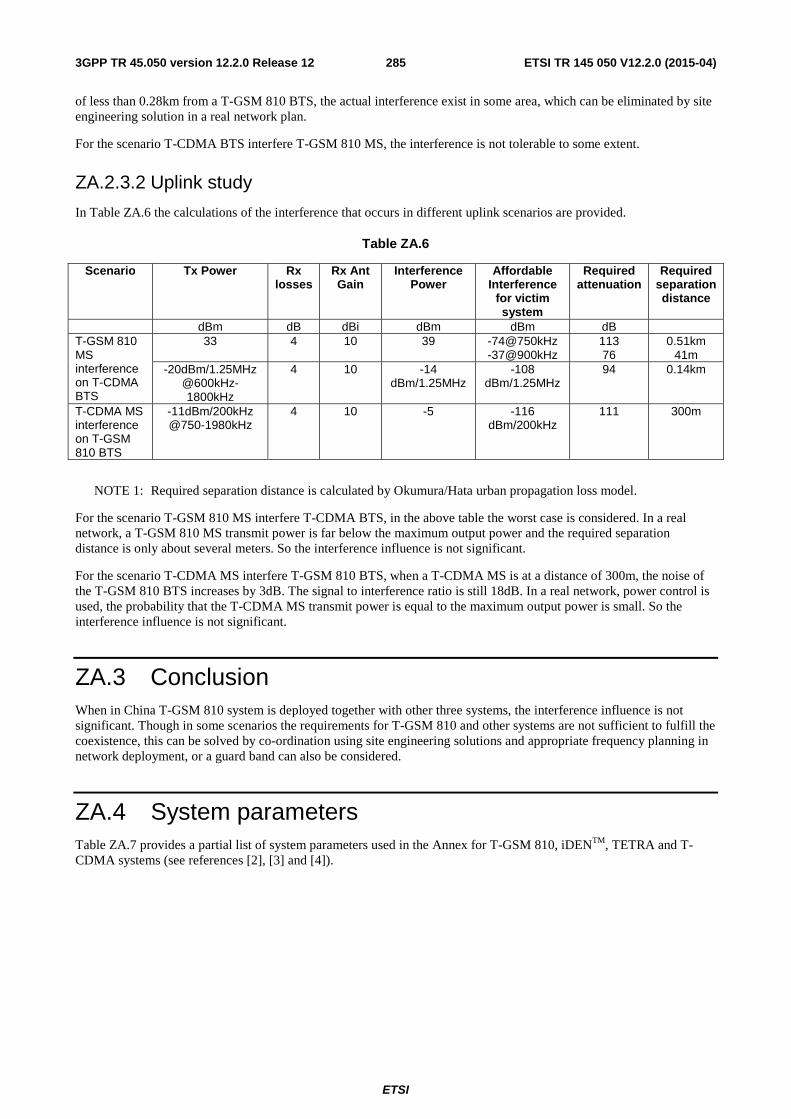
ZA.4 System parameters ................................................................................................................................ 285

ZA.5 References ............................................................................................................................................ 286

Annex ZB: Introduction of multicarrier BTS class ............................................................................. 287

ZB.1 Introduction .......................................................................................................................................... 287

ZB.2 Transmitter ........................................................................................................................................... 287

ZB.2.1 Introduction .................................................................................................................................................... 287

ZB.2.2 Proposal for relaxation and change ................................................................................................................ 288

ZB.2.2.1 Introduction of MCBTS class 1 and class 2 .............................................................................................. 288

ZB.2.2.2 Spectrum due to modulation and wideband noise..................................................................................... 288

ZB.2.2.3 Spurious emission ..................................................................................................................................... 288

ZB.2.2.4 BSS Intermodulation attenuation .............................................................................................................. 289

ZB.2.3 Simulation results ........................................................................................................................................... 289

ZB.2.4 Impact to GSM-R due to relaxation ............................................................................................................... 297

ZB.3 Receiver ................................................................................................................................................ 297

ZB.3.1 Proposal for the relaxation.............................................................................................................................. 297

ZB.3.2 Treatment of receive levels exceeding the new blocking limit....................................................................... 298

ZB.3.2.1 Simulation results ..................................................................................................................................... 298

ZB.3.2.2 Conclusion ................................................................................................................................................ 300

ZB.3.2.3 Discussion ................................................................................................................................................. 301

Annex ZC: Introduction of Medium Range and Local Area multicarrier BTS classes ................... 302

ZC.1 Introduction .......................................................................................................................................... 302

ZC.2 Transmitter ........................................................................................................................................... 302

ZC.3 Receiver ................................................................................................................................................ 302

ZC.4 References ............................................................................................................................................ 303

Annex ZD: ER-GSM band introduction ............................................................................................... 304

ETSI


ZD.1 Introduction .......................................................................................................................................... 304

ZD.2 Generalities on Working assumption and methodology ...................................................................... 304

ZD.2.1 Evaluation on impacted requirements ................................................................................................................. 304

ZD.2.2 Assumptions ................................................................................................................................................... 305

ZD.2.2.1 RF performances ....................................................................................................................................... 305

ZD.2.2.2 Blocker rejection by victim public base station ........................................................................................ 305

ZD.2.2.3 Blocking and Intermodulation reminders ................................................................................................. 306

ZD.2.2.4 Desensitization computing method ........................................................................................................... 306

ZD.2.2.5 Coordinated and uncoordinated deployment ............................................................................................ 307

ZD.2.2.6 Exception to blocking requirement for ER-GSM mobiles ........................................................................ 307

ZD.3 Victim receiver performance for lowest frequency offset of ER-GSM interferer................................ 307

ZD.3.1 GSM BTS as victim receiver .......................................................................................................................... 307

ZD.3.2 UTRA/E-UTRA BS as victim receiver .......................................................................................................... 308

ZD.4 Victim receiver performance in the ER-GSM frequency range ........................................................... 308

ZD.4.1 GSM BTS as victim receiver .......................................................................................................................... 309

ZD.4.2 UTRA/E-UTRA BS as victim receiver .......................................................................................................... 309

ZD.5 Specified requirement based on co-existence analysis ......................................................................... 309

ZD.5.1 Uncoordinated deployment ................................................................................................................................. 310

ZD.5.2 Coordinated deployment ..................................................................................................................................... 310

ZD.6 References ............................................................................................................................................ 310

Annex ZE: Extended TSC Sets .............................................................................................................. 311

ZE.1 Extended TSC Sets Design................................................................................................................... 311

ZE.1.1 Introduction .................................................................................................................................................... 311

ZE.1.2 Training Sequence Design .............................................................................................................................. 311

ZE.1.2.1 Initial Search ............................................................................................................................................. 311

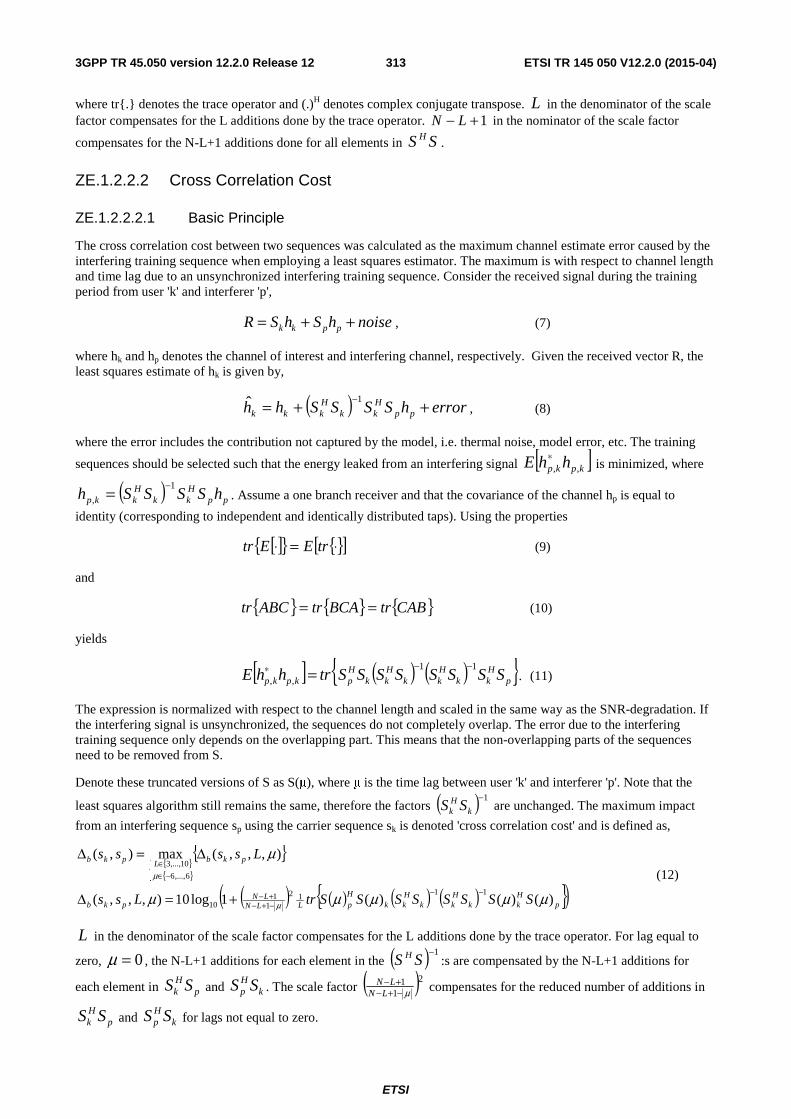
ZE.1.2.2 Building the Cost Function ....................................................................................................................... 312

ZE.1.2.2.1 Auto Correlation Cost ......................................................................................................................... 312

ZE.1.2.2.2 Cross Correlation Cost ........................................................................................................................ 313

ZE.1.2.2.2.1 Basic Principle ............................................................................................................................... 313

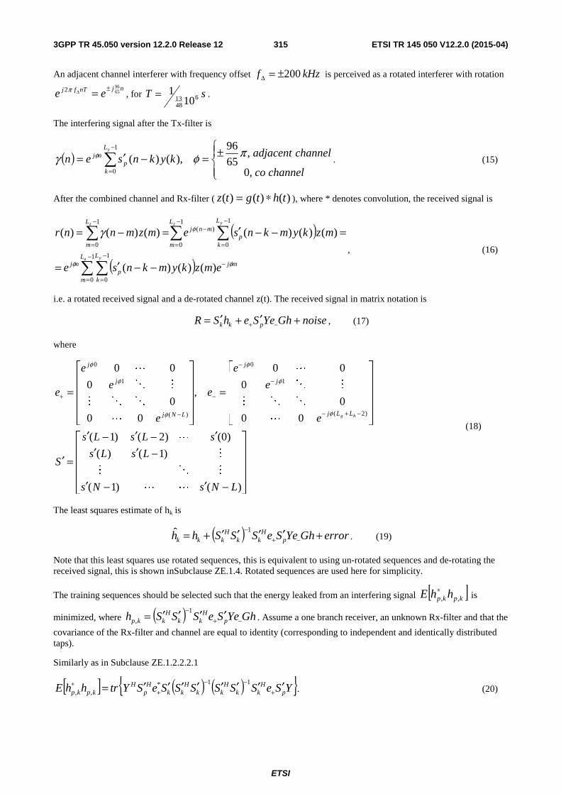
ZE.1.2.2.2.2 Used Model ................................................................................................................................... 314

ZE.1.2.3 Performing the search ............................................................................................................................... 317

ZE.1.3 Proposed Training Sequence Code Set ........................................................................................................... 317

ZE.1.4 Equivalence of rotational approaches ............................................................................................................. 318

ZE.2 Performance framework for design of Extended TSC Sets .................................................................. 320

ZE.2.1 Working Assumptions for performance framework ....................................................................................... 320

ZE.3 Delay statistics for design of Extended TSC Sets ................................................................................ 322

ZE.3.1 Background .................................................................................................................................................... 322

ZE.3.2 Simulations ..................................................................................................................................................... 323

ZE.3.2.1 Simulation assumptions ............................................................................................................................ 323

ZE.3.2.2 Non-ideal network synchronization .......................................................................................................... 323

ZE.3.2.3 Collection of results .................................................................................................................................. 324

ZE.3.2.4 Delay distribution ..................................................................................................................................... 324

ZE.4 NewToN – Performance evaluation ..................................................................................................... 324

ZE.4.1 Introduction .................................................................................................................................................... 325

ZE.4.2 Impact of co-TSC interference ....................................................................................................................... 325

ZE.4.2.1 Introduction............................................................................................................................................... 325

ZE.4.2.2 System model of co-TSC interference ...................................................................................................... 326

ZE.4.2.2.1 Network configuration ................................................................................................................................... 326

ZE.4.2.2.2 Interferer strength .......................................................................................................................................... 327

ZE.4.2.2.3 Co-TSC probability ....................................................................................................................................... 328

ZE.4.2.3 Link level simulations ............................................................................................................................... 329

ZE.4.2.3.1 Interference model ......................................................................................................................................... 329

ZE.4.2.3.2 Other simulation parameters .......................................................................................................................... 330

ZE.4.2.3.3 Results and discussion ................................................................................................................................... 330

ZE.4.3 System level simulations ................................................................................................................................ 330

ETSI


ZE.4.3.1 Introduction............................................................................................................................................... 330

ZE.4.3.2 Simulation assumptions ............................................................................................................................ 331

ZE.4.3.3 Results – non-VAMOS ............................................................................................................................. 331

ZE.4.3.4 Results – VAMOS .................................................................................................................................... 332

ZE.4.4 Performance comparison according to NewToN framework ......................................................................... 333

ZE.4.5 Conclusions .................................................................................................................................................... 334

ZE.4.6: Performance comparison according to NewToN performance framework ........................................................ 335

ZE.4.7 Detailed link level performance ..................................................................................................................... 336

Annex ZF: Change history .................................................................................................................... 337

History ............................................................................................................................................................ 338

ETSI


Foreword This Technical Report has been produced by the 3rd Generation Partnership Project (3GPP).

The contents of the present document are subject to continuing work within the TSG and may change following formal TSG approval. Should the TSG modify the contents of the present document, it will be re-released by the TSG with an identifying change of release date and an increase in version number as follows:

Version x.y.z

where:

x the first digit:

1 presented to TSG for information;

2 presented to TSG for approval;

3 or greater indicates TSG approved document under change control.

y the second digit is incremented for all changes of substance, i.e. technical enhancements, corrections, updates, etc.

z the third digit is incremented when editorial only changes have been incorporated in the document.

ETSI


1 Scope The present document gives background information on how the RF requirements of GSM400, GSM900 and DCS 1800 systems have been derived.

2 Information available The present document collects together temporary documents of ETSI SMG and STC SMG2 and 3GPP GERAN which can be seen as base line material for the RF requirements in GSM 05.05. The documents are divided into several clauses

In each clause there is a short description of the documents. The documents themselves are annexed to this report.

A list of phase 2 change requests to SMG2 related documents are annexed to the SMG meeting reports.

3 DCS1800 system scenarios There are two documents describing the basis of the DCS1800 RF requirements. They are:

- DCS1800 System scenarios (TDoc SMG 259/90, reproduced as TDoc SMG 60/91).

- Justifications for the DCS1800 05.05 (TDoc SMG 260/90, revised as TDoc SMG 60/91)).

These documents have been derived first by the UK PCN operators and later by GSM2 ad hoc group working on DCS 1800 requirements during 1990. The documents were presented to TC SMG in October 1990.

DCS1800 System Scenarios describes six scenarios which are considered to be the relevant cases for DCS1800. The six scenarios described are:

- Single MS - Single BTS.

- Multiple MSs - Multiple co-ordinated BTSs.

- Multiple MSs - Multiple uncoordinated BTSs.

- Co-located MSs, co-ordinated/uncoordinated.

- Co-located BTSs, co-ordinated/uncoordinated.

- Co-location with other systems.

On each of these scenarios the system constraints related to the scenario are described, the RF requirements affected by the scenario are identified and the input information needed to study the scenario in detail is listed.

Justifications for the DCS1800 05.05 includes the analysis of the system scenarios to detailed RF requirements and presents and justifies the proposed changes to GSM 05.05 for DCS1800. In the analysis part the relevant scenario calculations are made for each RF requirement and the most critical scenario requirement identified. The justification part then looks at the identified scenario requirement, compares it to the corresponding existing GSM900 requirement and taking also into account the implementation issues and finally gives reasoning to the proposed change of the specific RF requirement.

These documents are in annex A.

The DCS1800 requirements were originally developed for Phase 1 as a separate set of specifications, called DCS-specifications. For Phase two the DCS1800 and GSM900 requirements are merged. The main Phase 2 change requests of SMG2 in which the requirements for the DCS1800 system were included into are listed below.

- CR 05.01-04 Combination of GSM900 and DCS1800 specifications.

- CR 05.05-37 rev1 Combination of 05.05 (GSM900) and 05.05-DCS (DCS1800) specifications.

ETSI


- CR 05.08-55 rev1 Combination of GSM900 and DCS1800 and addition of National roaming.

Further development of the DCS1800 requirements for Phase 2 can be found in the other Phase 2 CRs of SMG2, the vast majority of which are valid both for DCS1800 and GSM900. The list of Phase 2 CRs of SMG2 can be found in annex E.

4 GSM900 small cell system scenarios There is one document which discusses the small cell system scenarios for GSM900. The document is:

- Small cell system scenarios for GSM900 (TDoc SMG2 104/92, revised as TDoc SMG2 104/92 rev1).

Small cell system scenarios for GSM900 uses the DCS1800 system scenarios and justification document and derives from them the scenario requirements for GSM900 small cells. It also calculates the worst case requirements based on minimum coupling loss of 59 dB.

The document on GSM900 small cell system scenarios is in annex B.

CR 03.30-02 on "Propagation models for different types of cells" gives a definition for a small cell and the typical cell parameters to calculate the propagation loss in a small cell.

5 GSM900 and DCS1800 microcell system scenarios GSM900 and DCS1800 microcells have been discussed by SMG2 in various meetings since late 1991. In SMG2#2 (May 1992) a small group was formed to collect together the various documents and make a proposal for the microcell RF parameters. As agreed by SMG2 there should be four microcell specific requirements, namely:

- transmit power;

- receive sensitivity;

- wideband noise;

- blocking.

As a result of the subgroup and other SMG2 activities there are three documents which can be used as baseline material for the microcell requirements. They are:

- Microcell BTS RF parameters (TDoc SMG2 163/92);

- Comments and proposals on Microcell RF parameters (TDoc 144/92);

- Revised proposal for microcell RF parameters (TDoc SMG2 ad hoc 4/92).

Microcell BTS RF parameters and Comments and proposals on Microcell RF parameters are joint papers giving the microcell scenarios and the requirements. The first one describes the two microcell scenarios, namely range and proximity, and presents the method to derive the detailed requirements starting from the scenarios. The latter document includes some corrections/updates to the scenarios, and proposes the detailed requirements. As described in the documents there are three classes of microcells, depending on the expected Minimum Coupling Loss between BTS and MS. This is to guarantee the optimum choice of BTS transmit powers while maintaining the operability of the system. The last of the microcell documents, Revised proposal for microcell RF parameters includes updates to the detailed requirement figures.

All the microcell requirements were collected together and were presented to and approved by SMG#5.

The documents on GSM900 and DCS1800 microcells are in annex C.

The relevant change requests where the detailed microcell requirements can be found, are listed below.

- CR 03.30-04 Microcell Radio planning aspects;

- CR 03.30-08 Microcell minimum coupling loss for small frequency offsets;

ETSI


- CR 05.05-69 rev1 Microcell BTS RF parameters;

- CR 05.05-79 rev1 Alignment of microcell maximum peak power requirement presentation;

- CR 05.05-90 Update of DCS1800 microcell RF parameters.

6 Conversion factors One of the tasks in ETSI/STC SMG2 has been to align the different RF requirements for the Phase 2 specifications. This was found necessary because in phase 1 some of the RF requirements dominated over others making them almost obsolete. Related to the alignment process it was found necessary to introduce a set of conversion factors to be able to compare different types of requirements measured with different measurement techniques. The original work assumptions were agreed on at SMG2#1 in February 1992 and they were reviewed in SMG2 ad hoc meeting in April 1992.

There are two documents related to the conversion factors. They are:

- Report of the ad hoc meeting on RF parameters (TDoc SMG2 61/92).

- Agreed SMG2 conversion factors (TDoc SMG2 287/92).

Report of the ad hoc meeting on RF parameters describes the process of deriving the conversion factors. In the ad hoc meeting there were number of input papers with practical measurement results of different measurement techniques, and in the ad hoc those measurement results were compared and the average of the results was chosen as a conversion factor. The following conversion factors were agreed on.

- conversion from maximum peak power to average power in a 30 kHz bandwidth on carrier:

=> -8 dB.

- conversion from average power to maximum peak power in 30 kHz bandwidth:

=> +8 dB at zero offset from carrier and + 9 dB at all other offsets.

- conversion from average power in 100 kHz bandwidth to maximum peak power in 30 kHz bandwidth:

=> +5 dB at offset above 1 800 kHz from carrier.

On the conversion factor from maximum peak power in 300 kHz bandwidth to maximum peak power in 30 kHz bandwidth no agreement was reached in the ad hoc meeting and hence the working assumption agreed on in SMG2 meeting is still assumed while pending for further validation.

=> -8 dB at offset above 6 MHz from the carrier.

Agreed SMG2 conversion factors lists the above agreed conversion factors and proposes further a conversion factor of +5 dB for conversions from 100 kHz bandwidth to 300 kHz bandwidth at offsets above 1 800 kHz from the carrier.

These documents are in annex D.

7 Repeaters There are a number of documents describing the background to repeater scenarios. These are:

- Repeater operating scenarios (Tdoc SMG2 29/94);

- Repeater scenarios for DCS1800 (Tdoc SMG2 24/94);

- Repeater scenarios (Tdoc SMG2 25/94);

- Repeater out of band gain (Tdoc SMG2-RPT 20/94).

Repeater operating scenarios: describes the many different scenarios for which a repeater device might be used.

ETSI


Repeater scenarios for DCS1800: describes two scenarios for DCS1800 repeaters, the outdoor scenario and the indoor scenario. For each scenario, the performance requirements on the repeater are derived.

Repeater scenarios: derives the equations that describe the uplink and downlink performance of a repeater. Co-ordinated and uncoordinated scenarios are analysed resulting in outline proposals for repeater hardware requirements in GSM 05.05 and outline planning guidelines in GSM 03.30.

Repeater out of band gain: derives the requirements for the repeater out of band gain and provides planning guidelines when a repeater is in close proximity to other communication systems.

These documents are in annex E.

The documents were presented to STC SMG2 in March 1994. In conclusion, it was decided that no single repeater specification would serve the large number of repeater scenarios that exist. As a consequence, it was agreed to add a specification for the repeater out of band performance to GSM 05.05 with guidelines for the specification and planning of repeaters in the GSM/DCS bands in GSM 03.30.

8 Error Patterns for Speech Coder Developments TD 164/95 in annex F describes available error patterns.

9 Simulations of Performance Several documents in annex G gives background information and simulation results of the GSM performance.

10 GSM900 railway system scenarios In 1993, the "Union Internationale de Chemin de Fer", UIC, decided to base a new railways pan-European system on GSM technology operating in the 900 MHz band.

In 1995, the CEPT, in recommendation T/R 25-09, decided that " the international requirements without excluding national requirements of railways for non-public digital radiocommunication system in the 900 MHz band should be covered by selecting appropriate sub-bands from the designated band 876 MHz to 880 MHz (mobile station transmit) paired with 921 MHz to 925 MHz (base station transmit) with a duplex separation of 45 MHz".

During 1996, SMG2 in a two-step process discussed the RF parameters in GSM 05.05 for GSM-type equipments operating in this frequency band, called UIC equipments. Two documents were elaborated for this purpose. They are:

- UIC system scenarios requirements;

- UIC RF parameters.

In UIC system scenarios requirements, the relevant system and interference scenarios for UIC equipments are identified and the noise levels allowed and the signal levels arising out of the worst cases are derived, both as regards intra-systems performance of a UIC network and towards other GSM-type systems in the neighbouring frequency bands.

Basing on the former, UIC RF parameters discusses all the parameters in GSM 05.05 and determines the RF requirements for UIC equipments, to be in line with the scenario requirements where possible and feasible, or being a reasonable compromise where not. The specifications for other GSM900 and DCS1800 types of equipment are not affected, except possibly where there is absolutely no implications for their implementation.

These documents are in clauses H.1 and H.2, respectively.

The resulting specifications were incorporated into GSM 05.05 by Change Request no. A027.

ETSI


11 Simulation results for GPRS receiver performance The documents in annexes K, L, M, N, P, Q and W give background information and simulation results of GPRS receiver performance

12 Pico BTS RF scenarios The documents in annex R give background information on pico BTS RF scenarios.

13 CTS system scenarios The document in annex S gives background information on CTS system scenarios.

14 GSM400 system scenarios There is one document describing the GSM400 system scenarios. The present document is:

- GSM400 system scenarios (Tdoc SMG2 190/99, revised as Tdoc SMG2 542/99).

GSM400 System Scenarios document presents GSM400 operation primarily in respect of the GSM 05.05 series of recommendations. All relevant scenarios for each part of GSM 05.05 are considered and the most critical cases identified. As a result the present document gives background information for GSM400 RF requirements presented in GSM 05.05 specification.

The present document on GSM400 system scenarios is in annex T.

15 MXM system scenarios The document in Annex U gives background information for 850 MHz and 1 900 MHz mixed mode system operation. 850 MHz and 1 900 MHz mixed-mode is defined as a network that deploys both 30 kHz RF carriers and 200 kHz RF carriers in geographic regions where the Federal Communications Commission (FCC) regulations are applied.

16 LCS scenarios The documents in annex V gives background information on LCS scenarios.

17 8-PSK Scenarios The document in annex X gives background information on 8-PSK scenarios.

18 T-GSM 900 System Scenarios The document in annex Y gives background information on T-GSM 900 scenarios.

19 MBMS System Scenarios The document in annex Z gives background information and simulation results of MBMS receiver performance.

ETSI


20 T-GSM 810 System Scenarios The document in annex ZA gives background information on coexistence scenarios for T-GSM810.

21 Multicarrier BTS Class The document in annex ZB gives background information on introduction of multicarrier BTS class.

22 ER-GSM band introduction As per the Work Item RT_ERGSM approved at 3GPP GERAN #51 in ZD.6 [1], it is required that investigations are performed to ensure that introduction of RF requirements for ER-GSM equipments usage will minimize the potential impacts to existing 3GPP systems in the E-GSM band and secure that the current 3GPP GERAN requirements of the existing GSM 900 bands and therefore dedicated equipment and services are not affected.

Annex ZD is therefore created to meet that requirement and gives background information on introduction of ER-GSM band scenarios.

23 Extended Training Sequence Code Sets

23.1 Background All burst types, except the frequency correction burst, contain a training sequence (also referred to as a synchronization sequence). Its purpose is to facilitate synchronization, channel estimation and blind detection of modulation on the radio interface.

For normal bursts (NB) and higher symbol rate bursts (HB) a set of eight training sequences is defined for each modulation (GMSK, 8PSK, 16QAM and 32QAM for NB, and QPSK, 16QAM and 32QAM for HB) to facilitate training sequence planning, i.e., avoiding that strong interfering bursts have the same training sequence as the wanted signal bursts.

For VAMOS, a second set of eight training sequences (TSC Set 2) is defined for GMSK modulated normal bursts (see 3GPP TS 45.002). Two GMSK training sequences are used to form the AQPSK training sequence (see 3GPP TS 45.002) for the downlink VAMOS modulation. The VAMOS (Set 2) training sequences have superior cross-correlation properties compared to the first set. This has facilitated improved Circuit Switched (CS) link level performance leading to enhanced BTS hardware capacity and improved spectral utilization in CS deployments compared to only using the existing TSC set.

All training sequences are defined in 3GPP TS 45.002.

23.2 Extended TSC Sets

23.2.1 Scope

When using extended TSC sets additional sets, each of eight training sequences, are defined for the different modulations when using normal bursts. The number of additional TSC sets depends on the domain (circuit switched or packet switched) they operate in and the modulation scheme used.

For the circuit switched domain, two new GMSK sets, referred to as GMSK TSC Set 3 and GMSK TSC Set 4 are defined. For VAMOS, the two GMSK training sequence sets can be used to form the AQPSK training sequence (see 3GPP TS 45.002) for the downlink VAMOS modulation.

For the packet switched domain, including EGPRS and EGPRS2-A, one additional set of eight training sequences is defined for each of GMSK, 8PSK, 16QAM and 32QAM normal bursts, referred to as TSC Set 2 for 8PSK, 16QAM and

ETSI


32QAM modulation, while for GMSK, TSC set 3, which is identical to TSC set 3 used for circuit switched channels, is used.

With 16 new sequences for GMSK and 8 new sequences for 8PSK, 16QAM and 32QAM a total of 40 new sequences are introduced.

23.2.2 Design criteria

The new sequences have good cross-correlation properties both within the sets for each modulation but also between the different modulations and towards all TSC sets that existed before the extention was introduced, for all modulations as well as the dummy burst. When designing the sequences, care was taken to make sure the cross correlation properties were especially good for co-channel interference, but also to have good properties for adjacent channel interference. With better cross-correlation properties the link level performance is improved and hence also the spectral efficiency for both the Packet Switched (PS) and the Circuit Switched (CS) domain. The gains will be most evident in the case of synchronous network operation, where the training sequence of wanted signal and interferer to a large extent overlap.

23.2.3 Design methodology

The design of the training sequences is described in detail in the document in Subclause ZE.1. The sets were derived one at a time in the order GMSK Set 3, GMSK Set 4, 8PSK Set 2, 16QAM Set 2, 32QAM Set 2. Each new set was designed such that the cross-correlation properties were good not only within the set but also towards all other existing sets, currently available, and the already generated extended TSC sets in the step-wise approacch.

First an exhaustive search was performed and a large number of sequences with good auto-correlation properties and good cross-correlation properties against all existing sets were selected. Measures of both auto-correlation and all combinations of cross-correlation for all these sequences were calculated. The set was then selected as the one minimizing the cost function based on these correlations.

23.2.4 Evaluation methodology

A methodology framework for evaluating the extended TSC set was followed according to the document in Subclause ZE.2. In short the extended TSC set was evaluated in both interference limited (including both CCI and ACI) and sensitivity limited scenario. For interference limited scenarios the relative delay of the interferer was derived using system level simulations with different cell sizes and re-use factors. The evaluation was based on simulations. These simulations covered both the CS and PS domain for the 900 MHz frequency band. All modulations, including GPRS, EGPRS and EGPRS2-A were considered. Besides sensitivity evaluations, co-channel and adjacent channel interference evaluations were performed. Both non-VAMOS and VAMOS test cases were included in the evaluation. Different weight factors were applied, to arrive at a final performance figure, depending on interference scenario and modulation used. For more details see the document in Subclause ZE.3. The working assumptions in Subclause ZE.3 constitute the basis of what is expected from the extended TSC sets. They are a set of rules defining not only how to evaluate the sets, but also highlighting what is considered to be important during the design of the sequences. Since the working assumptions describe what the extended TSC sets are designed for they are valuable to include in this document for future reference.

23.2.5 Performance evaluation

The performance evaluation, appended in Subclause ZE.4, show the gains of extending the TSC sets. For the performance evaluation a synchronous network has been assumed.

It is shown that increasing the TSC plan from 8 TSCs to 16 TSCs for speech channels give a link level gain of roughly 2 dB and a system capacity gain of 34 - 47 % because of the reduced probability of co-TSC interference and improved TSC correlation properties.

System level capacity gains with VAMOS have also been evaluated, see Subclause ZE.4, where additional gains compared to VAMOS when using existing TSC sets was shown to be 12 – 18 percentage points.

Evaluation of the extended TSC sets described in Section 23.2.3 has been performed according to the evaluation methodology described in Section 23.2.4 resulting in an average gain of 1.5 dB and 0.7 dB compared to TSC set 1, and TSC set 1 and 2 respectively.

ETSI


Annex A:DCS1800 System scenarios ETSI GSM TC TDoc GSM 259/90

Corfu, 1-5 October 1990

Source: GSM2 Ad Hoc on DCS1800, Bristol

Title: DCS1800 - System Scenarios

A.0 INTRODUCTION This paper discusses system scenarios for DCS1800 operation primarily in respect of the GSM 05.05 series of recommendations. To develop the DCS1800 standard, all the relevant scenarios need to be considered for each part of GSM 05.05 and the most critical case identified. The process may then be iterated to arrive at final parameters that meet both service and implementation requirements.

Each scenario has three sections:

a) lists the system constraints such as the separation of the MS and BTS, antenna height etc;

b) lists those sections of 05.05 that are affected by the constraints;

c) lists the inputs required to examine the implications of the scenarios.

The following scenarios are discussed:

1) Single MS, single BTS;

2) Multiple MS and BTS where operation of BTS's is coordinated;

3) Multiple MS and BTS where operation of BTS's is uncoordinated;

4) Colocated MS;

5) Colocated BTS;

6) Colocation with other systems.

A.1 SCENARIO 1 - SINGLE BTS AND MS

A.1.1 Constraints Aside from the frequency bands, the main constraint is the physical separation of the MS and BTS. The extreme conditions are when the MS is close to or remote from the BTS.

A.1.1.1 Frequency Bands and Channel Arrangement (Clause 2 of GSM 05.05)

The system is required to operate in the following frequency bands:

- 1 710 MHz to 1 785 MHz: mobile transmit, base receive;

- 1 805 MHz to 1 880 MHz: base transmit, mobile receive;

with a carrier spacing of 200 kHz.

ETSI


In order to ensure the compliance with the radio regulations outside the band, a guard band of 200 kHz between the edge of the band and the first carrier is needed at the bottom of each of the two subbands. Consequently , if we call F1(n) the nth carrier frequency in the lower band, and Fu(n) the nth carrier frequency in the upper band, we have:

- Fl(n) = 1710.2 + 0.2*(n-512) (MHz) (512 < n < 885)

- Fu(n) = Fl(n) + 95 (MHz)

The value n is called the ABSOLUTE RADIO FREQUENCY CHANNEL NUMBER (ARFCN). To protect other services, channels 512 and 885 will not normally be used, except for local arrangements.

A.1.1.2 Proximity

Table 1 shows examples of close proximity scenarios in urban and rural environments. Different antenna heights are considered; 15 m high antennas are assumed to have lower gain (10 dBi) than 30 m high antennas (18 dBi).

Table 1: Worst case proximity scenarios

Rural Urban Building Street Building Street (note 1) (note 1)

BTS height, Hb (m) 20 15 15 30 30

MS height, Hm (m) 1,5 15 1,5 20 1,5

Horizontal separation (m) (note 4) 30 30 15 60 15 BTS antenna gain, Gb (dB) (note 2) 18 10 10 18 18

BTS antenna gain, G'b (dB) (note 3) 0 10 2 13 0

MS antenna gain, Gm (dB) 0 0 0 0 0

Path loss into building (dB) 6 6 Cable/Connector Loss (dB) 2 2 2 2 2 Body Loss (dB) 1 1 1 1 1 Path loss - antenna gain (dB) 71 66 65 69 71 NOTE 1: Handset at height Hm in building. NOTE 2: Bore-sight gain. NOTE 3: Gain in direction of MS. NOTE 4: Horizontal separation between MS and BTS.

Path loss is assumed to be free space i.e. 37,5 + 20 log d(m) dB, where d is the length of the sloping line connecting the transmit and receive antennas.

These examples suggest that the worst (ie lowest) coupling loss occurs in urban areas where the MS is in a street below the BTS. The coupling loss is then 65 dB. The coupling loss is defined as that between the transmit and receive antenna connectors.

A.1.1.3 Range

Table 2 shows examples of range scenarios. The ranges quoted are the maximum anticipated for DCS1800 operation. In rural areas, this implies relatively flat terrain with little foliage loss. In urban areas, up to 1 km cells should be supported. In each case, an allowance must be made for in-building penetration loss. The figures shown are examples of those needed to achieve these cell sizes. In many situations, however, smaller cells may be used depending on the local conditions of terrain and traffic demand.

ETSI


Table 2: Worst case range scenarios

Rural Urban BTS height, Hb (m) 60 50

MS height, Hm (m) 1,5 1,5

BTS antenna gain, Gb (dB) 18 18

MS antenna gain, Gm (dB) 0 0 Path loss into building (dB) [10] [15] Target range (km) 8 1

A.1.2 05.05 Paragraphs Affected

Paragraph Title 2 Frequency bands and channel arrangement

4.1 Output power 6.1 Nominal error rates (maximum receiver levels) 6.2 Reference sensitivity level

A.1.3 Inputs needed Working assumptions

Propagation model Hata model (down to 1 km)

Free space (up to [200] m maximum)

Log normal shadow margin [6] dB

Building penetration loss - urban [15] dB

- rural [10] dB

External noise (continuous and impulsive) Negligible

MS noise figure: [12] dB

BTS noise figure: [8] dB

Ec/No: 6 dB + 2 dB (implementation margin)

Location probability, Ps: 75% at cell boundary

Implementation losses

Body loss [3] dB (typical)

A.2 SCENARIO 2 - MULTIPLE MS AND BTS, COORDINATED

Coordinated operation is assumed ie BTS's belong to same PLMN. Colocated MS's and colocated BTS's are dealt with in Scenarios 4 and 5, respectively.

A.2.1 Constraints The constraints are the same as those for scenario 1.

ETSI


A.2.2 05.05 paragraphs affected

Paragraph Title 4.1 Adaptive power control:

- reduces co- and adjacent- channel interference. - controls near/far effect for multiple MS's to same BTS.

4.2 Output RF spectrum: - to limit adjacent channel interference.

4.3 Spurious emissions (in-band): - near/far effect to same BTS. - see figure 2.1.

4.5 Output level dynamic operation: - near/far effect to same BTS. - required limits comparable with spurious.

4.7.1 Intermodulation attenuation, BTS - see figure 2.2.

4.7.2 Intra BTS intermodulation attenuation: - see figure 2.3.

5.1 Blocking, in-band: - near/far effect.

6.3 Reference interference level

A.2.3 Inputs needed Target Cluster size Assume 9 cell, i.e. 3 site, 120° sectored.

Figure 2.1: Near/far effect

3 cell, 120° sectored BTS; 400 kHz channel separation between; sectors; 30 dB BTS transmitter/receiver coupling; or transmitter/transmitter coupling.

Figure 2.2: Scenario for Intermodulation distortion

ETSI


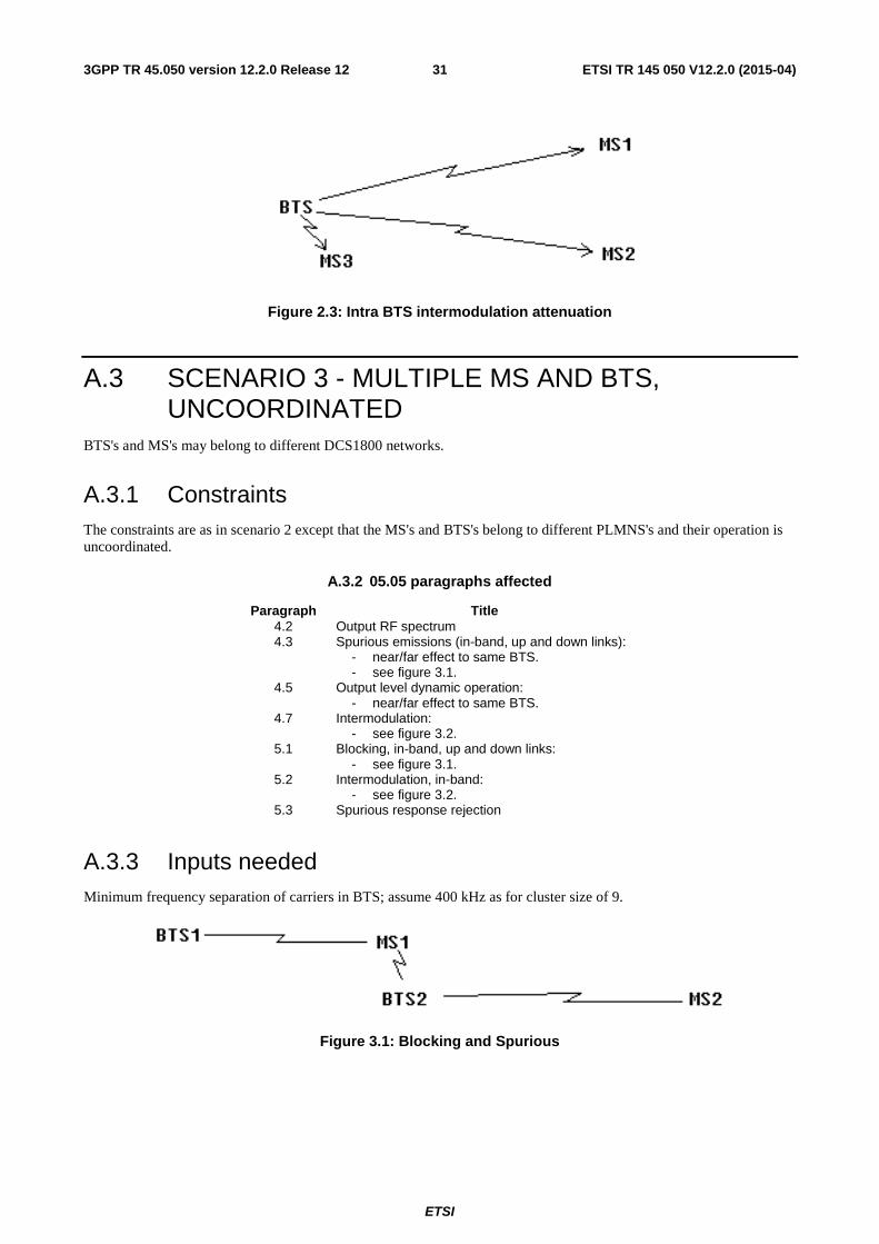
Figure 2.3: Intra BTS intermodulation attenuation

A.3 SCENARIO 3 - MULTIPLE MS AND BTS, UNCOORDINATED

BTS's and MS's may belong to different DCS1800 networks.

A.3.1 Constraints The constraints are as in scenario 2 except that the MS's and BTS's belong to different PLMNS's and their operation is uncoordinated.


Paragraph Title 4.2 Output RF spectrum 4.3 Spurious emissions (in-band, up and down links):

- near/far effect to same BTS. - see figure 3.1.

4.5 Output level dynamic operation: - near/far effect to same BTS.

4.7 Intermodulation: - see figure 3.2.

5.1 Blocking, in-band, up and down links: - see figure 3.1.

5.2 Intermodulation, in-band: - see figure 3.2.

5.3 Spurious response rejection

A.3.3 Inputs needed Minimum frequency separation of carriers in BTS; assume 400 kHz as for cluster size of 9.

Figure 3.1: Blocking and Spurious

ETSI


BTS1 and BTS2 belong to different PLMN's. MS1 affiliated to BTS1 PLMN; MS2 and MS3 affiliated to BTS2 PLMN.

Intermodulation products in BTS1 receiver.

Figure 3.2: Intermodulation

A.4 SCENARIO 4 - COLOCATED MS Colocated MS which may be served by BTS from different networks ie MS's not synchronised.

A.4.1 Constraints Minimum separation of MS 1 m.

Guard band between up and down links 20 MHz.

Bandwidth of up and downlink bands 75 MHz.


Paragraph Title 4.3.3 Spurious emissions, out-of-band. 5.1 Blocking, out-of-band. 5.3 Spurious response rejection. 5.4 Spurious emissions.

[New 4.7.3 Intermodulation between MS]. - see figure 4.1.

ETSI


Out-of-band intermods; MS1 and MS2 at full power. Received signal at MS3 from BTS2 at reference sensitivity. By symmetry, MS1 will be affected by an I.M.

product from MS2 and MS3 whenever MS3 is affected as shown above.

In-band intermods.

Figure 4.1: Intermodulation between MS

A.4.3 Inputs needed Additional body losses; assume [3 dB].

A.5 SCENARIO 5 - COLOCATED BTS Two or more colocated BTS possibly from different PLMN's.

A.5.1 Constraints Coupling between BTS's may result either from the co-siting of BTS's or from several BTS's in close proximity with directional antenna. The maximum coupling between BTS' should be assumed to be [30] dB. This is defined as the loss between the transmitter combiner output and the receiver multi-coupler input.


Paragraph Title 4.3 Spurious emissions.

4.7.1 Intermodulation attenuation, BTS: - (see figure 5.1).

5.1 Blocking: - [30] dB coupling between BTS TX - RX. - [30] dB coupling between BTS TX - TX. - [30] dB coupling between BTS RX - RX. - BTS either same or different PLMN.

5.3 Spurious response rejection. 5.4 Spurious emissions.

A.5.3 Inputs needed None.

ETSI


BTS3 different PLMN from BTS 1 and 2. Intermodulation products at MS3 receiver.

Figure 5.1: Intermodulation scenario

A.6 SCENARIO 6 - COLOCATION WITH OTHER SYSTEMS

DCS1800 systems will have to work in the presence of other mobile radio systems.

A.6.1 Constraints Operation of DCS1800 mobiles to be considered in close proximity with other systems.

GSM phase 1;

GSM phase 2;

DECT;

Analogue cellular (TACS, NMT450/900, C450, R2000); and

CT2 mobiles.


Paragraph Title 4.3 Spurious emissions, out-of-band 5.1 Blocking, out-of-band 5.3 Spurious response rejection 5.4 Spurious emissions

A.6.3 Inputs needed Performance specifications of other systems.

ETSI


ETSI GSM TC TDoc GSM 60/91

Saarbrucken, 14-18 January 1991

Source: GSM2

A.7 Title: Justifications for the proposed Rec. 05.05_DCS

I INTRODUCTION

The DCS1800 system requirements are defined in a paper entitled 'DCS1800 - System Scenarios' (GSM TDoc 259/90) and the parameters chosen either meet these requirements or represent a compromise between them and what can be manufactured at an appropriate cost. Changes to the 900 MHz standard have only been made where there is a specific system advantage or cost saving. Consideration has been given to methods of measurement for the changed specifications.

Section II expands the scenarios paper into more detailed requirements for RF parameters. Section III follows the section numbering of GSM 05.05 and justifies the desired changes for DCS1800. The present document does not comment on simple changes from GSM900 to DCS1800 frequency bands since this change is assumed.

II METHODOLOGY

Unless otherwise stated the results of scenario calculations assume transmit powers of 39 dBm for the base and a 30 dBm for the mobile, both measured at their respective antenna connectors. The equivalent noise bandwidth of the transmitted signal is taken to be 120 kHz and that of the receiver 180 kHz. Worst case scenarios usually involve a "near/far" problem of some kind, the component scenario assumptions (as given in the scenarios paper for "near" and "far" can be summarised as follows.

"Near" Coupling loss (dB) BTS -> MS 65 MS -> BTS 65 MS-> MS 40.5

BTS -> BTS 30 The coupling loss is defined between antenna connectors. The powers and sensitivities are discussed in section III of this paper, they are quoted here to enable scenario calculations to be performed. The transmitter power and receiver sensitivity are measured at the respective antenna connectors.

"Far" Tx power (dBm) Rx Sensitivity (dBm) BTS 39 -104 MS 30 -100

Scenarios can involve uncoordinated or co-ordinated entities (MS or BTS) depending on whether they are from the same PLMN. With uncoordinated operation handover and power control are not used in response to the proximity of the BTS and more severe near/far problems can arise, however, co-ordinated scenarios are often more likely spatially and more likely to occur at lower frequency offsets. Unco-ordinated scenarios become critical when they involve mobiles being simultaneously on the edge of their serving cell and close to another operator's BTS, also the transmitter and affected receiver will be in different operator frequency allocations. It is most important that the co-ordinated scenario requirements are met where possible.

The probability and consequences of the various scenarios must be taken into account when choosing the actual specification. For example, jamming a whole base station is a more serious consequence than jamming a single mobile and intermodulation scenarios which involve the co-location of 3 entities are consequently less likely than those which only involve 2.

ETSI


The remainder of this section outlines the key scenario calculations which affect the choice of parameters for GSM 05.05. Transmitted levels are those in the receiver bandwidth, although in many cases the test bandwidths are narrower because of the need to avoid switching transients affecting the measurement.

A.7.1 Transmitter

A.7.1.1 Modulation, Spurs and Noise

A.7.1.1.1 Co-ordinated, BTS -> MS (Scenario 2, figure 2.1)

Since the affected MS is close to its own base we only need to ensure adequate C/I at the BTS.

Max. Tx noise level in Rx bandwidth = [BTS power] - [Power control range] - [C/I margin] - [Multiple interferers margin] = 39 - 30 - 9 - 10 = -10 dBm.

(BTS dynamic power control is optional, in the worst case it will be employed on the link to the affected MS but the other link will be at full power).

A.7.1.1.2 Uncoordinated, BTS -> MS (Scenario 3, figure 3.1)

Max. Tx. level of noise in Rx. bandwidth = [MS sensitivity] - [C/I margin] - [Multiple interferers margin] + [Coupling loss] = -100 - 9 -10 + 65 = -54 dBm.

Max. Tx level of spur in Rx bandwidth = [MS sensitivity] - [C/I margin] + [Coupling loss] = -100 - 9 + 65 = -44 dBm.

A.7.1.1.3 Co-ordinated & Uncoordinated MS -> BTS (Scenarios 2 and 3, figures 2.1 and 3.1)

Max. Tx level in Rx bandwidth = [BTS sensitivity] - [C/I margin] + [Coupling loss] = -104 - 9 + 65 = -48 dBm.

Although the absolute spec. is the same the MS may find it easier to meet scenario 2 because it will be powered down.

A.7.1.1.4 Co-ordinated & Uncoordinated MS->MS (Scenario 4)

Max Tx level in Rx bandwidth = [MS sensitivity] - [C/I margin] + [Coupling loss] = -100 - 9 + 40.5 = -68.5 dBm.

A.7.1.1.5 Co-ordinated & Uncoordinated BTS->BTS (Scenario 5)

Max Tx level noise in Rx bandwidth= [BTS sensitivity] - [C/I margin] - [Multiple interferers margin] + [Coupling loss] = -104 - 9 - 10 + 30 = -93 dBm.

A.7.1.2 Switching Transients

The peak level of transients in a 5 pole synchronously tuned measurement filter of bandwidth 100 kHz simulates their effect on the receiver. The transients only effect a few bits per timeslot and have approximately 20 dB less effect than continuous interference. Their peak level falls off at 20 dB decade both with increasing frequency offset and measurement bandwidth.

A.7.1.2.1 Uncoordinated MS -> BTS (Scenario 3, figure 3.1)

Max. peak level in effective Rx BW at MS = [Base sensitivity] - [C/I margin] + [Coupling loss] + [Transient margin] = -104 - 9 +65 + 20 = -28 dBm.

A.7.1.2.2 Uncoordinated BTS -> MS (Scenario 3, figure 3.1)

Max. peak level in effective Rx BW at BTS = [MS sensitivity] - [C/I margin] + [Coupling loss] + [Transient margin] = -100 - 9 + 65 + 20 = -24 dBm.

ETSI


A.7.1.3 Intermodulation

A.7.1.3.1 Co-ordinated, BTS -> MS (Scenario 2, figures 2.2 and 2.3)

(Level of input signal 30 dB below wanted transmission).

Required IM attenuation in BTS = [C/I margin] + [BTS power control range] + [margin for other IMs] = 9 + 30 + 3 = 42 dB.

A.7.1.3.2 Uncoordinated, BTS ->MS (Scenario 3, figure 3.2 top)

(Level of input signal 30 dB below wanted transmission).

Required IM attenuation in BTS = [BTS power] - {[Max. allowed level at MS1] + [coupling loss BTS2->MS1]} = 39 -{{-100 - 9 - 3} + 65} = 86 dB.

A.7.1.3.3 Uncoordinated, MS&MS-> BTS (Scenario 4, figure 4.1 bottom)

(Level of input signal 40,5 dB below wanted transmission).

Required IM attenuation in MS = [MS power] - {[Max. allowed level at BTS2] + [coupling loss MS->BTS2]} = 30 -{{-104 - 9 - 3} + 65} = 81 dB.

A.7.1.3.4 Uncoordinated MS&MS-> MS (Scenario 4, figure 4.1 top)

(Level of input signal 40,5 dB below wanted transmission).

Required IM attenuation in MS = [MS power] - {[Max. allowed level at MS3] + [coupling loss MS->MS3]} = 30 -{{-100 - 9 - 3} + 40,5} = 101,5 dB.

A.7.2 Receiver

A.7.2.1 Blocking

A.7.2.1.1 Co-ordinated & Uncoordinated BTS-> MS (Scenarios 2 and 3, figures 2.1 and 3.1)

Max. level at MS receiver = [BTS power] + [Multiple interferers margin] - [Coupling loss] = 39 + 10 - 65 = -16 dBm.

A.7.2.1.2 Co-ordinated MS-> BTS (Scenario 2, figure 2.1)

Max level at BTS receiver = [MS power] - [Power control range] - [Coupling loss] = 30 - 20 - 65 = -55 dBm.

A.7.2.1.3 Uncoordinated MS-> BTS (Scenario 3, figure 3.1)

Max level at BTS receiver = [MS power] - [Coupling loss] = 30 - 65 = -35 dBm.

A.7.2.1.4 Co-ordinated & Uncoordinated MS-> MS (Scenario 4)

Max. level at MS receiver = [MS power] - [Coupling loss] = 30 - 40,5 = -10,5 dBm.

A.7.2.1.5 Co-ordinated & Uncoordinated BTS-> BTS (Scenario 5)

Max. level at BTS receiver = [BTS power] + [Multiple interferers margin] - [Coupling loss] = 39 +10 - 30 = 19 dBm.

ETSI


A.7.2.2 Intermodulation

A.7.2.2.1 Co-ordinated & Uncoordinated BTS-> MS (Scenarios 2 and 3, figure 3.2 middle)

Max. received level at MS1 = [BTS power] - [Coupling loss BTS2->MS1] + [Margin for other IMs] = 39 - 65 + 3 = -23 dBm.

Required IM attenuation in MS is 42 dB for scenario 2 and 86 dB for scenario 3. TheGSM 05.05 clause 5.2 test simulates scenario 3.

A.7.2.2.2 Co-ordinated MS & MS -> BTS (Scenario 4)

Max. received level at BTS1 = [MS power] - [MS power control range] - [Coupling loss MS-> BTS1] + [Margin for other IMs] = 30 - 20 - 65 + 3 = -52 dBm.

A.7.2.2.3 Uncoordinated MS & MS -> BTS (Scenario 4, figure 3.2 lower)

Max. received level at BTS1 = [MS power] - [Coupling loss MS-> BTS1] + [Margin for other IM's] = 30 - 65 + 3 = -32 dBm.

A.7.2.3 Maximum level

A.7.2.3.1 Co-ordinated MS -> BTS (Scenario 1)

Max level at BTS = [MS power] - [Coupling loss] = 30 - 65 = -35 dBm.

(The BTS must be capable of decoding the RACH which is at full power).

A.7.2.3.2 Co-ordinated BTS -> MS (Scenario 1)

Max level at MS = [BTS power] - [Coupling loss] = 39 - 65 = -26 dBm.

(BTS dynamic power control is optional, in the worst case it will not be employed, also the MS must be capable of decoding the BCCH carrier).

III JUSTIFICATIONS

A.8.1 SCOPE

A.8.2 FREQUENCY BANDS AND CHANNEL ARRANGEMENT The up and downlink frequencies have been changed to cover the 1,8 GHz band. The 374 carrier frequencies have been assigned ARFCNs starting at 512.

A.8.3 REFERENCE CONFIGURATION

ETSI


A.8.4 TRANSMITTER CHARACTERISTICS

A.8.4.1 Output power

A.8.4.1.1 Mobile Station

MS power classes of 1 and ¼W have been chosen for DCS1800 defined in the same way as for GSM900. With a 30 m antenna height Hata's model predicts that the higher MS power class will not quite meet the target ranges given in the system scenarios paper both for urban and rural areas. The requirement for a cheap, small, low power handset is also an important constraint. It is felt that the chosen power classes represent a reasonable compromise between these conflicting requirements.

A 20 dB power control range has been chosen for both classes of mobile since it is believed that this will give most of the available improvement in uplink co-channel interference.

Since the chosen power classes and hence power control levels are even numbers in dBm they will not fit into the existing numbering scheme, so a new one has been used. These numbers are only of editorial significance.

The absolute tolerance on power control levels below 13 dBm has been increased by:

- 1 dB because of manufacturers' concerns about implementation.

A.8.4.1.2 Base Station

Following GSM900, the BTS power classes are specified at the combiner input. In order to provide the operator some flexibility four power classes have been specified in the range 34 dBm to 43 dBm. In fact the four lowest power classes from GSM900 have been retained although the numbering has been changed. The 39 dBm BTS power measured at the antenna connector might typically match a 30 dBm mobile.

The tolerance on the BTS static power control step size has been relaxed to simplify implementation, control of the BTS power to an accuracy of less than 1dB was felt to be unnecessary.

The penultimate paragraph has been reworded because a class 1 mobile no longer has 15 power steps.

A.8.4.2 Output RF spectrum

The BTS is not tested in frequency hopping mode. If the BTS uses baseband frequency hopping then it would add little to test in FH mode; if it uses RF hopping then the test will be complicated by permissible intermodulation products (see subclause 4.7) from BTSs which do not de-activate unallocated timeslots.

A.8.4.2.1 Spectrum due to the modulation

The relaxation for MSs with integral antennas has been removed.

The measurement has been extended to cover the whole transmit band and beyond 1 800 kHz from carrier measurements are only taken on DCS1800 carrier frequencies using a 100 kHz bandwidth. This technique still avoids permissible switching transients, is fairly quick and closely reflects the receiver bandwidth and hence the system scenario. It is now a measurement of broadband noise as well as modulation.

The technique proposed in CR 30 for counting spur exceptions in FH mode for GSM 05.05 is also included here.

The table has been split into those parts which apply to the mobile and those which apply to the base reflecting the difference in their respective scenario requirements.

When operating at full power, the table below shows the frequency offset at which scenario requirements are met.

ETSI


39 dBm BTS at ant. conn. 30 dBm MS Scenario 2 400 kHz (1.1.1) 400 kHz (1.1.3) Scenario 3 missed by 10dB

at 6 MHz (1.1.2) 6 MHz (1.1.3)

The figures in brackets are the relevant scenario requirement sub-section numbers in section II of the present document.

Exceptions i and ii below the table define the maximum number of exception channels appropriate to the frequency bands tested. For the BTS permissible intermodulation products must be avoided.

Since the table entries are relative, as the power level of the transmitter is reduced, the absolute specification becomes tighter. Exceptions iii and iv stop the transmitters having to exceed the requirement of scenario 3. Further relaxations are permitted at low frequency offsets; for the MS scenario 3 is unlikely below 600 kHz and the requirement of scenario 2 is used; for the BTS, the 10 dB multiple interferers margin is excessive below 1 800 kHz and the minimum level is increased by 5 dB.

A.8.4.2.2 Spectrum due to switching transients

a) Mobile Station

The table has been modified in accordance with the new mobile power classes. The transients are always above the modulation at 400 kHz offset and so the table collapses to a single row.

Requirement 1.2.1 for scenario 3 becomes -38,5 dBm in 30 kHz. The current specification meets this requirement at offsets above 2.4 MHz while the 4.2.1 test only meets scenario 3 at offsets above 6 MHz. The specification on transients is not the limiting case and need not be changed.

b) Base Station

Requirement 1.2.2 for scenario 3 becomes -34,5 dBm in 30 kHz. With the current specification a 39 dBm BTS meets this requirement at 600 kHz. Again no change is proposed. This figure assumes that "dBc" means relative to the on-carrier power in 30 kHz; a possible ambiguity in the wording has been removed.

A.8.4.3 Spurious emissions

A.8.4.3.1 Principle of the specification

Although 4.2.1 now covers the whole transmit band, the in band part of 4.3.1 is still required to check the behaviour of switching transients beyond 1800 kHz and to catch any spurs missed in 4.2.1.

A.8.4.3.2 Base Station

The protection of frequencies outside the DCS1800 band is unchanged, but the spurious emissions in the transmit band are only permitted up to -36 dBm which is below the CEPT limit of -30 dBm but the same as GSM 05.05. The same applies to the MS transmit band in 4.3.3. The new base receive band is given the same protection as before measured in the modified conditions of 4.2.1, this meets scenario requirement 1.1.5 scaled to a measurement bandwidth of 100 kHz. The GSM900 base receive band is also protected but only when the co-siting of GSM and DCS BTSs occurs.

A.8.4.3.3 Mobile Station

This section consists of two blanket specifications one for transmit mode and one for idle mode Specific tests of the MS receive band are also given.

When allocated a channel, the transmit band and out-of-band specifications are the same as for the BTS in 4.3.2. These are consistent with 4.2.1 and the CEPT specifications for spurious emissions.

In idle mode the CEPT specification below 1 GHz is also applied to the DCS transmit and receive bands using a 100 kHz measurement bandwidth, this specification also exceeds scenario requirement 1.1.3 for the MS transmit band. however, the number of mobiles in idle mode may be quite large.

ETSI


The test of the MS receive band meets scenario requirement 1.1.4 and uses the modified conditions of 4.2.1. 5 exception channels are permitted for discrete spurious, it is rather unlikely that two MS will be one metre apart and receiving at one of these exception channels. Protection of the GSM900 MS receive band is also provided. The specification is 6 dB tighter reflecting the reduced propagation loss between colocated MS at 900 MHz. The dependence of this test on power class has been removed since all mobiles are hand portables. No extra testing of the MS receive band in idle mode is made because it is unlikely to be worse than when allocated a channel.

A.8.4.4 Radio frequency tolerance

A.8.4.5 Output level dynamic operation

A.8.4.5.1 Base station

This specification only affects the interference experienced by co-channel cells in the same PLMN. The requirement on the relative power level of unactivated timeslots has been relaxed from -70 dBc to -30 dBc in line with the BTS power control range. It is understood that "dBc" includes the static but not dynamic power control.The specification has been extended to cover the whole transmit band because the residual power may not be highest on carrier.

The measurement bandwidth is specified as at least 300 kHz due to problems with ringing of the measurement filter just after an active burst has finished.

A.8.4.5.2 Mobile station:

The power level between active bursts from the MS affects the serving BTS receiver. The power measured in 100 kHz on carrier will be similar to that measured in the receiver bandwidth which must be less than -48 dBm to meet scenario requirement 1.1.3. The absolute specification has been tightened from -36 dBm to -47 dBm in line with this requirement but the relative specification has been retained. Allowing 10 dB for the peak-to-mean ratio of the power between active bursts if it is noise-like, the relative specification will meet this scenario requirement for a 1W MS.

A.8.4.6 Phase accuracy

A.8.4.7 Intermodulation attenuation

The definition of intermodulation attenuation has been moved from subclause 4.7.1 to subclause 4.7 to make it clear that it applies to subclauses 4.7.1, 4.7.2 and 4.7.3. A note concerning possible problems with VHF broadcast signals has been added because these are at the difference between the DCS up and downlink frequencies.

A.8.4.7.1 Base transceiver station

A.8.4.7.2 Intra BTS intermodulation attenuation

A.8.4.7.3 Intermodulation between MS

Section 4.7.3 of the 900 MHz specification concerned the mobile PBX. The mobile PBX is no longer included in GSM 02.06, there is no type approval for it and consequently the original subclause 4.7.3 text has been removed. The new section 4.7.3 relates to intermodulation between MS transmitters, an area which was not covered in the 900 MHz standard.

In the proposed measurement, the level of the interfering signal simulates that from a very close MS and the required IM attenuation is to protect MS or BS receivers in the vicinity. MS transmit intermods are covered by scenario requirements 1.3.3 and 1.3.4. If the product lands in the BTS receive band 81 dB IM attenuation is required, if the product lands in the MS receive band 101,5 dB IM attenuation is required in the MS transmitter which produces the IM.

Both these scenarios require the co-location of 3 objects (MS or BTS) with the correct frequency relationship. Experiments performed by manufacturers on 900 MHz PA's indicate that 50 dB attenuation is achievable at all frequency offsets. A tighter specification would require the use of an isolator or more linearity in the PA design. A specification of 50 dB tested at 800 kHz offset was agreed.

ETSI


A.8.5 RECEIVER CHARACTERISTICS A clarification of the of the measurement point for the receiver specifications in line with that for the transmitter has been made.

A.8.5.1 Blocking characteristics

The MS blocking specification close to the received channel has not been changed, this is limited by the receive synthesizer phase noise. At higher frequency offsets the blocking specification relates to the DCS1800 band and the feasibility of the receive filter. The proposed specification is shown below, the dashed line shows a possible receive filter frequency response.

The blocking specification at > 3 MHz offset in the receive band misses the scenario requirement 2.1.1 (-16 dBm) by 10 dB, but the transmit band specification meets scenario requirement 2.1.4 (-10,5 dBm). Power consumption considerations make it undesirable to tighten the receive band specification. The outside the DCS1800 band the 0 dBm specification has been retained. The combination of these proposals amounts to a filter specification over the MS receive band as shown below.

The BTS blocking requirement has been significantly relaxed because the MS power classes are lower. Scenario requirement 2.1.2 is -55 dBm which considers blocking from the bases own MS's. Requirement 2.1.3 is -35 dBm which is for mobiles from other operators. The proposal meets the scenario requirements even at 600 kHz offset and exceeds it by 10 dB beyond 800 kHz.

The consequence of failing to meet this scenario is that the whole base station is blocked. For this reason it is desirable for the base station to exceed the scenario requirement if possible.

The out-of-band specification has not been changed, although it does not meet scenario requirement 2.1.5 (19 dBm). This is because the 30 dB coupling loss assumption between base stations is rather pessimistic, it corresponds to two 18 dBi antennas on boresight 17 m apart. Under these circumstances, operators may need to adopt specific mutual arrangements (eg. extra operator specific receive filters) which need not form part of the DCS1800 standard.

-28

-24

-20

-16

-12

-8

-4

0

1680 1700 1720 1740 1760 1780 1800 1820 1840 1860 1880 1900 1920 1940 1960 1980 2000

Lev

el d

Bm

ETSI


A.8.5.2 Intermodulation characteristics

The 900 MHz standard for handportables limits the maximum level to -49 dBm. Any tightening of this specification will increase the power consumption of the receiver. Since DCS1800 is designed for handportables this figure is now applied to all MSs. The proposed level of -49 dBm for the MS fails to meet scenario requirement 2.2.1 by 23 dB, but the only consequence is that the MS is de-sensed when close to a BTS with the appropriate transmitters active.

The worst case for BTS receiver IMs is when two MSs approach the base, the scenario requirement is covered in subclauses 2.2.2 and 2.2.3 and is -55 dBm for co-ordinated mobiles and -35 dBm for uncoordinated.

Again -49 dBm has been proposed since the probability of the uncoordinated scenario is low both spatially and spectrally. If the coupling loss between both MSs and the BTS increases by 1dB the level of a third order IM product will reduce by 3 dB, thus if the coupling loss assumption between MS and BTS is increased by 5 dB to 70 dB then the scenario would be met.

A note concerning the VHF broadcast problem has been added as in subclause 4.7 for transmiiter intermodulation.

A.8.5.3 Spurious response rejection

This section concerns exceptions to the blocking specification due to spurs in the receive synthesizer and mixer causing spurious responses. The numbers of exception channels has been doubled to reflect the wider receive band. For the BTS the in-band blocking specification can cover frequency offsets of 95 MHz depending on the receive frequency and including the 20 MHz extension of the receive band defined in subclause 5.1. Thus the boundary between parts a and b of the specification has been moved from 45 MHz to 95 MHz because the receive band is now 50 MHz wider.

Following the above logic the breakpoint between parts a and b for the MS should occur at -95 MHz and +115 MHz but in the interests of simplicity the same breakpoint is proposed as for the BTS.

A.8.5.4 Spurious emissions

Since the MS receiver spurious emissions are covered by the idle mode aspect of 4.3.3 this section now only refers to the BTS.

A.8.6 TRANSMITTER/RECEIVER PERFORMANCE

A.8.6.1 Nominal error rates (NER)

The scenario requirement for the maximum received level at the MS is -26 dBm (requirement 2.3.2). The figure of -23 dBm is also in approximate alignment with the blocking specification at >3 MHz.

The required NER for the static channel above at -23 dBm has been increased to ½% in line with CR 28

Under multipath conditions the peak signal level exceeds the mean level. In order to prevent significant clipping the maximum level under multipath conditions has been set to -40 dBm. Multipath reception conditions occur when there is no line of sight path and the received signal level is likely to be lower.

The same specifications have been applied to the BTS receiver.

A.8.6.2 Reference sensitivity level

Simulations of TU50 and HT100 at 1,8 GHz have been performed and table 1 has been modified appropriately. The RA130 results at 1,8 GHz are taken from the RA250 results at 900 MHz. Allowance has been made for enhanced bad frame indication in accordance with CR 27.

The MS sensitivity has been relaxed by 2 dB to simplify the MS at the expense of a slightly higher BTS power requirement, to balance the up and downlinks.

ETSI


A.8.6.3 Reference interference level

TU1.5 and RA 130 results at 1,8 GHz in table 2 are taken from TU3 and RA250 in GSM 05.05 respectively. TU 50 at 1,8 GHz has been simulated and the results are incorporated in the table. Allowance has been made for enhanced bad frame indication in accordance with CR 27.

The effect of doubling the Doppler spread is in general to improve the performance without FH due to increased decorrelation between bursts and to slightly degrade performance with FH because the channel is less stationary during the burst.

A.8.6.4 Erroneous frame indication performance

ETSI


Annex B: GSM900 Small Cell System scenarios

ETSI/STC/SMG2 T.Doc 104/92 - Rev. 1

Strasbourg

1 - 4 September 1992

Title: Small Cell System Scenarios for GSM900.

Source: Vodafone, UK

Introduction

Small cells are defined in GSM 03.30 as having antennas above median roof height but below maximum, whereas Large cells have antennas above the maximum roof height. Median roof heights vary with location, in particular between City Centre and Suburban locations. Suburban median roof heights vary with type of housing and may often be characteristic of a particular country but are likely to fall between 8 m and 20 m.

Small cells feature much lower antennas than large cells and as such the minimum coupling loss between base and mobile antenna is significantly decreased. In practice small cells are likely to operate at a lower transmit power level, being aimed at providing limited coverage, but not necessarily capacity, in urban/suburban environments.

This paper presents the results of applying the propagation loss at 100m BTS to MS antenna separation from the GSM 03.30 Small Cell example, to the system scenarios in TDoc GSM 61/91 which details system scenarios for DCS1800. The results are presented in a similar manner as TDoc GSM 60/91 and will be applicable to a 75% location probability.

A further set of results is presented for the worst case scenario where the agreed Minimum Coupling Loss (MCL) of 59 dB from T.Doc SMG 49/91 is used.

Both sets of results assume a Class 2 coordinated and uncoordinated MS but the effect of MS power control is taken into account for the coordinated MS.

Small Cell Example

The definition of the small cell example in GSM 03.30 annex A.4 is as follows.

Base TX Configuration Antenna Gain: +16 dBi (BAG) Antenna Height: 17 m Roof Height 15 m Antenna Feeder Loss: 2 dB (BFL)

Mobile RX Configuration Antenna Gain: 2 dBi (MAG) Antenna Height 1,5 m Antenna Feeder Loss: 2 dB (MFL)

Propagation Loss Loss (dB) = 132,8 + 38 log(d/km)

The coupling loss for this scenario is then:

132,8 + 38 log(d/km) - BAG + BFL - MAG + MFL= 80,8 dB at a MS to base separation of 100 m.

The system scenarios at 100 m are presented in Appendix 1.

Minimum Coupling Loss Case

ETSI


The system scenarios based on the same small cell example as above but using a MCL of 59 dB are presented in Appendix 2.

It should be noted that this produces worse case figures, assuming operation at limit sensitivity, i.e. in a noise limited environment. For the small cell case the MS at least, is likely to be operating in an interference limited environment with an effective sensitivity worse than limit sensitivity.

Appendix 1: System Scenarios for Small Cell GSM900

Near Coupling loss BTS -> MS 81 MS -> BTS 81 MS -> MS 34,5

BTS -> BTS 25

Far Tx power (dBm Rx Sensitivity (dBm) BTS 38 -104 MS 39 -104

BTS power control range 30 MS power control range 26 C/I margin 9 Multiple interferers margin 10 Transient margin 20 margin for other IMs 3

NOTE: All results are in dBm except for subclause 1.3 where the results are dB.

B.1 Transmitter

B.1.1 Modulation, Spurs and Noise

B.1.1.1 Co-ordinated, BTS -> MS

Max. Tx noise level in RX bandwidth = [BTS power] - [Pwr control range] - [C/I margin]-[Multiple interferers margin] = -11.

B.1.1.2 Uncoordinated, BTS -> MS

Max Tx level of noise in Rx bandwidth = [MS sensitivity] - [C/I margin] - [multiple interferers margin] + [coupling loss] = -42.

Max Tx level of spur in Rx bandwidth = [MS sensitivity] - [C/I margin] + [coupling loss] = -32.

B.1.1.3 Co-ordinated & Uncoordinated MS -> BTS

Max Tx level in Rx bandwidth = [BTS sensitivity] - [C/I margin] + [coupling loss] = -32.

B.1.1.4 Co-ordinated & Uncoordinated MS -> MS

Max Tx level in Rx bandwidth = [MS sensitivity] - [C/I margin] + [Coupling loss] = -78,5.

ETSI


B.1.1.5 Co-ordinated & Uncoordinated BTS -> BTS

Max Tx level noise in Rx bandwidth = [BTS sensitivity] - [C/I margin] - [multiple interferers margin] + [coupling loss] = -98.

B.1.2 Switching Transients

B.1.2.1 Uncoordinated MS -> BTS

Max peak level in effective Rx BW at MS = [Base sensitivity] - [C/I margin] + [coupling loss] + [Transient margin] = -12.

B.1.2.2 Uncoordinated BTS -> MS

Max peak level in effective Rx BW at BTS = [MS sensitivity] - [C/I margin] + [coupling loss] + [transient margin] = -12.

B.1.3 Intermodulation

B.1.3.1 Coordinated, BTS -> MS

Required IM attenuation in BTS = [C/I margin] + [BTS pwr control range] + [margin for other IMs] = 42.

B.1.3.2 Uncoordinated, BTS -> MS

Required IM attenuation in BTS = [BTS power] - {[Max allowed level at MS1] + [coupling loss BTS2 -> MS1]} = 73.

NOTE: [Max allowed level at MS1] = [MS sensitivity - C/I margin - margin for other IMs].

B.1.3.3 Uncoordinated, MS&MS -> BTS

Required IM attenuation in MS = [MS power] - {[Max allowed level at BTS2] + [coupling loss MS -> BTS2]} = 74.

NOTE: [Max allowed level at BTS2] = [BTS sensitivity - C/I margin - margin for other IMs].

B.1.3.4 Uncoordinated MS&MS -> MS

Required IM attenuation in MS = [MS power] - {[Max allowed level at MS3] + [coupling loss MS -> MS3]} = 120,5.


B.2 Receiver

B.2.1 Blocking

B.2.1.1 Co-ordinated & Uncoordinated BTS -> MS

Max level at MS receiver = [BTS power] + [multiple interferers margin] - [coupling loss] = -33.

B.2.1.2 Co-ordinated MS -> BTS

Max level at BTS receiver = [MS power] - [Power control range] - [coupling loss] = -68.

ETSI


B.2.1.3 Uncoordinated MS -> BTS

Max level at BTS receiver = [MS power] - [coupling loss] = -42.

B.2.1.4 Co-ordinated & Uncoordinated MS -> MS

Max level at MS receiver = [MS power] - [coupling loss] = 4,5.

B.2.1.5 Co-ordinated and Uncoordinated BTS -> BTS

Max level at BTS receiver = [BTS power] + [multiple interferers margin] - [coupling loss] = 23.

B.2.2 Intermodulation

B.2.2.1 Co-ordinated & Uncoordinated BTS -> MS

Max received level at MS1 = [BTS power] - [coupling loss BTS2->MS1] + [margin for other IMs] = -40.

B.2.2.2 Co-ordinated MS & MS -> BTS

Max received level at BTS1 = [MS pwr] - [MS pwr control range] - [coupling loss MS -> BTS1] + [margin for other IMs] = -65.

B.2.2.3 Uncoordinated MS & MS -> BTS

Max. received level at BTS1 = [MS power] - [coupling loss MS -> BTS1] + [Margin for other IMs] = -39.

B.2.3 Maximum level

B.2.3.1 Co-ordinated MS -> BTS

Max level at BTS = [MS power] - [coupling loss] = 42.

B.2.3.2 Co-ordinated BTS -> MS

Max level at MS = [BTS power] - [coupling loss] = -43.

Appendix 2: System Scenarios for Small Cell GSM900. 59 dB MCL

Near Coupling loss BTS -> MS 59 MS -> BTS 59 MS -> MS 34,5

BTS -> BTS 25

Far Tx power (dBm) Rx Sensitivity (dBm) BTS 38 -104 MS 39 -104

ETSI


BTS power control range 30 MS power control range 26 C/I margin 9 Multiple interferers margin 10 Transient margin 20 margin for other IMs 3

NOTE: All results are in dBm except for subclause 1.3 where the results are dB.

B.3.1 Transmitter

B.3.1.1 Modulation, Spurs and Noise

B.3.1.1.1 Co-ordinated, BTS -> MS

Max. Tx noise level in RX bandwidth = [BTS power] - [Pwr control range] - [C/I margin] - [Multiple interferers margin] = -11.

B.3.1.1.2 Uncoordinated, BTS -> MS

Max Tx level of noise in Rx bandwidth = [MS sensitivity] - [C/I margin] - [multiple interferers margin] + [coupling loss] = -64.

Max Tx level of spur in Rx bandwidth = [MS sensitivity] - [C/I margin] + [coupling loss] = -54.

B.3.1.1.3 Co-ordinated & Uncoordinated MS -> BTS

Max Tx level in Rx bandwidth = [BTS sensitivity] - [C/I margin] + [coupling loss] = -54.

B.3.1.1.4 Co-ordinated & Uncoordinated MS -> MS

Max Tx level in Rx bandwidth = [MS sensitivity] - [C/I margin] + [Coupling loss] = -78,5.

B.3.1.1.5 Co-ordinated & Uncoordinated BTS -> BTS

Max Tx level noise in Rx bandwidth = [BTS sensitivity] - [C/I margin] - [multiple interferers margin] + [coupling loss] = -98.

B.3.1.2 Switching Transients

B.3.1.2.1 Uncoordinated MS -> BTS

Max peak level in effective Rx BW at MS = [Base sensitivity] - [C/I margin] + [coupling loss] + [Transient margin] = -.34

B.3.1.2.2 Uncoordinated BTS -> MS

Max peak level in effective Rx BW at BTS = [MS sensitivity] - [C/I margin] + [coupling loss] + [transient margin] = -34.

ETSI


B.3.1.3 Intermodulation

B.3.1.3.1 Coordinated, BTS -> MS

Required IM attenuation in BTS = [C/I margin] + [BTS pwr control range] + [margin for other IMs] = 42.

B.3.1.3.2 Uncoordinated, BTS -> MS

Required IM attenuation in BTS = [BTS power] - {[Max allowed level at MS1] + [coupling loss BTS2 -> MS1]} = 95.


B.3.1.3.3 Uncoordinated, MS&MS -> BTS

Required IM attenuation in MS = [MS power] - {[Max allowed level at BTS2] + [coupling loss MS -> BTS2]} = 96.

NOTE: [Max allowed level at BTS2] = [BTS sensitivity - C/I margin - margin for other IMs].

B.3.1.3.4 Uncoordinated MS&MS -> MS

Required IM attenuation in MS = [MS power] - {[Max allowed level at MS3] + [coupling loss MS -> MS3]} = 120,5.


B.3.2 Receiver

B.3.2.1 Blocking

B.3.2.1.1 Co-ordinated & Uncoordinated BTS -> MS

Max level at MS receiver = [BTS power] + [multiple interferers margin] - [coupling loss] = -11.

B.3.2.1.2 Co-ordinated MS -> BTS

Max level at BTS receiver = [MS power] - [Power control range] - [coupling loss] = -46.

B.3.2.1.3 Uncoordinated MS -> BTS

Max level at BTS receiver = [MS power] - [coupling loss] = -20.

B.3.2.1.4 Co-ordinated & Uncoordinated MS -> MS

Max level at MS receiver = [MS power] - [coupling loss] = 4,5.

B.3.2.1.5 Co-ordinated and Uncoordinated BTS -> BTS

Max level at BTS receiver = [BTS power] + [multiple interferers margin] - [coupling loss] = 23.

B.3.2.2 Intermodulation

B.3.2.2.1 Co-ordinated & Uncoordinated BTS -> MS

Max received level at MS1 = [BTS power] - [coupling loss BTS2->MS1] + [margin for other IMs] = -18.

ETSI


B.3.2.2.2 Co-ordinated MS & MS -> BTS

Max received level at BTS1 = [MS pwr] - [MS pwr control range] - [coupling loss MS -> BTS1] + [margin for other IMs] = -43.

B.3.2.2.3 Uncoordinated MS & MS -> BTS

Max. received level at BTS1 = [MS power] - [coupling loss MS -> BTS1] + [Margin for other IMs] = -17.

B.3.2.3 Maximum level

B.3.2.3.1 Co-ordinated MS -> BTS

Max level at BTS = [MS power] - [coupling loss] = 20.

B.3.2.3.2 Co-ordinated BTS -> MS

Max level at MS = [BTS power] - [coupling loss] = -21.

ETSI


Annex C: Microcell System Scenarios ETSI STC SMG2 No.3 T Doc SMG2 63 /92

lst- 4th September 1992

Strasbourg

Source: BTL (UK)

Subject: Microcell BTS RF Parameters

Background

Since the Ronneby meeting of SMG2 there have been a number of input papers concerning the specification of RP parameters for a microcell BTS. In particular T.Docs 184/91, 16/92, 28/92, 80/92, 86/92 and 90/92 from AT&T NSI, MPC, BTL and Alcatel propose specific RF parameters. At the Turin SMG2 meeting it was agreed that the best way to include a microcell BTS specification into the GSM recommendations was as an annex to GSM 05.05 that would specify:

- Transmit powers.

- Receive sensitivities.

- Wideband noise.

- Blocking.

It was also agreed that it would not be practical to specify a single microcell BTS for all applications and that a number of BTS classes would need to be specified. It was noted that this may require guidelines to be added to 03.30 to ensure successful operation.

Scenario Requirements

In order to clarify the requirements for microcell BTS RF parameters we must first look at the scenario requirements. It was agreed at the Amsterdam meeting that the 2 groups of scenarios were 'range' and 'close proximity' as shown in figure 1.

Range:

The general requirements of the range scenario are that:

- Maximum BTS receive sensitivity is required for some applications.

- The uplink and downlink paths should be capable of being balanced.

It has been agreed that the COST 231 propagation model will be used for microcell propagation when a fine of sight street canyon exist. This has been included in GSM 03.30 for guidance (T.Docs 88/92 and 93/92). In order to estimate the maximum, worst case path loss experienced by a microcell BTS we would also have to define.

Table 2: Close Proximity Parameters

GSM900 DCS1800 Minimum Coupling Loss (MCL) 44 dB 50 dB Multiple Interferers Margin (MIM) 10 dB 10 dB C/I margin 9 dB 9 dB

Before we can calculate the scenario requirements shown in figure 1 we must identify some further MS RF parameters in addition to those in table 1.

ETSI


Table 3: Further MS RF Parameters

GSM900 (class 5) DCS1800 (class 1) Most stringent blocking requirement -23 dBm -26 dBm Wideband noise emission in 200 kHz -44 dB -48 dB

NOTE: Currently no specification for GSM900 MS wideband noise beyond 1,8 MHz offset and therefore figures proposed at Aalborg meeting used (as shown in T.Doc 11 1/92).

The wideband noise figures in table 3 have been adjusted by 3 dB since they are specified in a 100 kHz bandwidth in GSM 05.05 but are required in a receiver bandwidth for the scenarios (200 kHz).

BTS Tx power

This requirement (as shown in figure 1) is the maximum microcell BTS transmit power that can be tolerated in order to prevent MS blocking.

BTS Tx power = [MCL] ~ [blocking requirement].

GSM900 BTS Tx power = 44 + (-23) = 21 dBm.

DCS1800 BTS Tx power = 50 + (-26) = 24 dBm.

BTS wideband noise

This requirement (as shown in figure 1) is the maximum microcell BTS wideband noise that can be tolerated in order to prevent MS 'noise masking'. A signal lever lOdB above limit sensitivity is taken.

BTS wideband noise (in 100 kHz) = [signal lever] - [C/I margin] - [MIM] + [MCL] - [200 - 100 kHz BW conversion].

GSM900 BTS wideband noise = (-92) - 9 - 10 + 44 -3 = -70 dBm DCS1800 BTS wideband noise = (-90) - 9 - 10 + 50 -3 = -62 dBm.

- Non fine of sight propagation model.

- Log normal fading margin.

- Rician fading margin.

- Corner attenuation.

- Building penetration loss.

To find the range from this path loss we would have to define the link budget parameters such as antennae gains and cable losses. It is thought to be impractical to define all these parameters as part of this work. However, if we substitute some approximate numbers for the above parameters (such as those in T.Doc 80/92) we can see that with -104 dBm receive sensitivity at the microcell BTS worst case ranges could still be as low as 200 m to 300 m.

In order to define relationships for path balancing we need only to identify the mobile RF parameters and any differences in the uplink and downlink paths (e.g. diversity). The assumptions made here are:

- Class 5 MS for GSM900 and Class 1 MS for DCS1800.

- Same antennae used for transmit and receive at MS and BTS (therefore gain cancers).

- No diversity.

- Path balancing performed for maximum MS transmit power (to give absolute max. BTS transmit power required).

The following MS RF parameters are used:

ETSI


Table 1: MS RF Parameter

MS Tx power MS Rx sensitivity GSM900 29 dBm -102 dBm DCS1800 30 dBm -100 dBm

For balanced paths the uplink max path loss must equal the downlink max path loss. In other words:

[MS Tx power] + [-BTS Rx sens] = [BTS Tx power] + [-MS Rx sens].

The following relationships can therefore be defined:

GSM900 [BTS Tx power] + 73 = - [BTS Rx sensitivity].

DCS1800 [BTS Tx power] + 70 = - [BTS Rx sensitivity].

Close Proximity

At the Amsterdam microcell sub-group the Minimum Coupling Losses (MCL) for Microcell BTS to MS coupling were agreed (T.Doc 41/92 Rev 1). Further work showed that these figures were very worst case and had a low probability of occurring (T.Doc 90/92). The following parameters will be used in the close proximity scenarios.

BTS blocking

This requirement (as shown in Fig. 1) is the maximum signal lever that may be presented to a microcell BTS from an uncoordinated MS.

BTS blocking level = [MS Tx power] - [MCL].

GSM900 BTS blocking level = 29 - 44 = -15 dBm.

DCS1800 BTS blocking level = 30 - 50 = -20 dBm.

BTS Rx sensitivity

This requirement (as shown in figure 1) is the maximum receive sensitivity a microcell BTS can have in order to prevent 'noise masking' from an uncoordinated MS.

BTS Rx sensitivity = [wideband noise from MS] + [C/I margin] - [MCL].

GSM900 BTS Rx sensitivity = -44 + 9 - 44 = -79 dBm.

DCS1800 BTS Rx sensitivity = ~8 + 9 - 50 = -89 dBm.

Practical specification

So far, we have identified the requirements for the range and close proximity scenarios for a microcell BTS. We now need to move towards a practical specification.

Microcell BTS Tx power and Rx sensitivity

If we study the scenario requirements for transmit power and receive sensitivity we find the following:

- The Rx sensitivities needed to satisfy the close proximity scenarios are much less those required for the range scenarios.

- The Tx powers and Rx sensitivities from the close proximity scenarios lead to a 15 dB downlink bias for GSM900 and a 5 dB downlink bias for DCS1800.

In order to satisfy both the path balance relationships in the range scenario and the close proximity scenarios we can either reduce the Tx power or reduce the Rx sensitivity even further. Since the Rx sensitivity is well short of the range requirements already we shall choose to balance paths by reducing Tx power. This gives the following Tx powers:

GSM900 BTS Tx power = -(-79) + 73 = 6 dBm.

DCS1800 BTS Tx power = -(-89) + 70 = 19 dBm.

ETSI


However, if we want to specify microcell BTS classes with better Rx sensitivities than these (and hence higher Tx powers) then the value for MCL has to be increased in order to ensure the close proximity scenarios are satisfied. Popular Rx sensitivities to choose in order to optimise microcell BTS size and cost are -89 Bm and -95 dBm (from SMG2 input papers). Since the limiting close proximity scenario is MS wideband noise masking the microcell BTS receiver we must use this to determine the new MCL requirements as follows:

MCL = [wideband noise from MS] + [C/I margin] - [BTS Rx sensitivity].

Having clone this we can path balance to find the new Tx powers. These results are shown in table 4.

Table 4: New MCLs with balanced Rx sens and Tx powers

MCL Rx sens Tx power GSM900 44 dB -79 dBm 6 dBm 54 dB -89 dBm 16 dBm 60 dB -95 dBm 22 dBm 69 dB -104 dBm 31 dBm DCS1800 50 dB -89 dBm 19 dBm 56 dB -95 dBm 25 dBm 65 dB -104 dBm 34 dBm

Microcell blocting

It has been agreed that by reducing the Rx sensitivity we do not want to imply a relaxation in the blocking requirements for the microcell BTS. Therefore the blocking values will simply be increased by the same amount as the Rx sensitivity has decreased.

Table 5 Change in blocking requirement

Rx sens Change in blocking values

GSM900 -79 dBm +25 dB -89 dBm +15 dB -95 dBm +9 dB -104 dBm No change DCS1800 -89 dBm +15 dB -95 dBm +5 dB -104 dBm No change

Microcell BTS wideband noise

The scenario requirement for wideband noise will obviously change with the MCL. The wideband noise specification currently in GSM 05.05 is -80 dBc at greater than 6 MHz offsets. For low Tx power BTSs a noise floor of -57 dBm is specified for DCS1800 and 45 dBm (>6 MHz) for GSM900. Table 6 shows the scenario requirements for wideband noise with the -80 dBc values (relative to the microcell. Tx power - not shown) and the current specification values (i.e. either the -80 dBc or the noise floor value).

Table 6: Wideband noise requirements

MCL Scenario Requirement

-80 dBc values Current Spec

GSM900 44 dB 70 dBm -74 dBm -45 dBm 54 dB -60 dBm -64 dBm -45 dBm 60 dB -54 dBm -58 dBm -45 dBm 69 dB -45 dBm -49 dBm -45 dBm DCS1800 50 dB -62 dBm -61 dBm -57 dBm 56 dB -56 dBm -55 dBm -55 dBm 65 dB -47 dBm -46 dBm -46 dBm

ETSI


It can be seen that for DCS1800 the current specification satisfies the scenario requirements. However, for GSM900 there is up to a 25 dB discrepancy. A noise floor of -60dBm is proposed for GSM900 which would change the specification to -60 dBm, -60 dBm, -58 dBm and -49 dBm in the top right hand 4 boxes of table 6. This meets the scenario requirement in three cases and exceeds it by 10 dB in one case.

Proposed changes to GSM recommendations

The following changes have been Proposed to GSM 05.05.

Table 7: Microcell BTS Classes

Microcell BTS Class

Tx power (dBm)

Rx sensitivity Blocking (rel to current)

GSM900 1 31 -104 No change 2 22 -95 +9 dB 3 16 -89 +15 dB 4 6 -79 +25 dB DCS1800 1 34 -104 No change 2 25 -95 +9 dB 3 19 -89 +15 dB

Although the longer classes came from the original MCL figures it is recommended that certainly the GSM900 Class 4 BTS be removed as not practical and possibly both Class 3 BTSs also. This is open for discussion.

We have also shown that:

- The GSM900 MS wideband noise needs specifying to the band edge (as for DCS1800 MSs) with values at least as good as those proposed in Aalborg.

- The wideband noise floor for GSM900 microcell BTSs needs to be -60 dBm. No change is required for DCS1800.

The following additions are proposed to GSM 03.30.

The recommended MCL values for the different microcell BTS classes should be included in GSM 03.30 for guidance on installation. These MCL values are connector to connector values and therefore include antennae effects. The following should be added.

Table 8: Recommended MCLs

Microcell BTS Class Recommended MCL (dB)

GSM900 1 69 2 60 3 54 4 44 DCS1800 1 65 2 56 3 50

Removing the GSM900 Class 4 BTS would eliminate the 44 dB MCL from the table. It can be seen that higher MCLs are needed for GSM900 than for DCS1800. This will translate into even larger separations in the field due to the 6 dB fall in path loss when moving from 1,8 GHz to 900 MHz The only way to restore this balance is to specify a tighter MS wideband noise specification for GSM900 than that proposed in Aalborg.

ETSI


Figure 1

BTS

BTS

BTS

Blocking

Rx Sens WB Noise

Tx Pwr

UPLINK

DOWNLINK

MaxPathLoss

MCL

Microcell BTS parametersto be defined

MS paramters are known

Microcell BTS Scenarios

MCL

Rx Sens

Rx Sens

Rx SensWB Noise

Blocking

Tx Pwr

Tx Pwr

Tx Pwr

Close Proximity

Range

ETSI


ETSI/STC SMG 2 T.doc.144/92

Strasbourg, 1-4 September 1992

Source: Mercury Personal Communications

Title: Comments and Proposals on Microcell RF Parameters

Having read the paper from BTL on this subject and as a result of discussions with the author, the following additional comments and proposals have been agreed with him.

1) uBTS classes can be defined to meet MCLs in 5 dB steps GSM {45, 50, 55, 60} DCS {50, 55, 60}. This will aid the cell planner and manufacturers in choosing appropriate equipment for a given ucell site. It is also simpler.

2) Since DCS1800 r.f. parameters were defined using the scenarios approach used here for microcells, a DCS uBTS with a sensitivity of -104 dBm will be identical to a permitted normal BTS and there is therefore little point in defining it.

3) Diversity is possible in ucells. I suggest we allow 3 dB for this in the uBTS maximum power.

4) Parameters which affect the uBTS receiver should meet the MCL. Those which only affect the closest mobile can miss the MCL by 10 dB. The Telia research measurements (SMG2 T.doc. 90/92) show that this 10 dB translates a 0,1% probability to 10% probability of interference.

5) uBTS blocking should exceed the MCL requirement by 10 dB.

a) To allow for interfering signals from outside the system.

b) Because the consequences of the BTS being blocked are severe.

c) To improve the MCL performance with MSs which exceed their noise spec.

Proposed Procedure for Defining the Parameters (Similar to the BTL paper)

1) Choose uBTS sensitivity to match MS noise at MCL.

2) Choose uBTS power to balance links.

3) Set uBTS noise and blocking to be the same as for a normal BTS relative to the power and sensitivity respectively.

4) Relax the uBTS noise and blocking where possible to the point where it just meets the MCL requirements.

Spread Sheets giving uBTS RF Parameters (figures 1 to 3)

1) Microcell RF parameters proposed by BTL paper.

2) Parameters after stages 1-3 in the procedure above.

3) Proposed parameters after stages 1-4 above.

The final proposals are in figure 3. Notice that the class 1 uBTS can be converted into a class 2 with the addition of 5 dB attenuators on transmit and receive paths.

ETSI


Baseline Normal Class 1 Class 2 Class 3 Class 4

Normal Class 1 Class 2 Class 3

GSM DCS GSM GSM GSM GSM GSM DCS DCS DCS DCS

C/ I 9 9 9 9 9 9 9 9 9 9 9 BTS MIM 10 10 10 10 10 10 10 10 10 10 10 MS Margin 10 10 10 10 10 10 10 10 10 10 10 BTS Div. Gain 0 0 0 0 0 0 0 0 0 0 0

MS Power 29 30 29 29 29 29 29 30 30 30 30 MS Noise -44 -48 -44 -44 -44 -44 -44 -48 -48 -48 -48 MS Blocking -23 -26 -23 -23 -23 -23 -23 -26 -26 -26 -26 MS Sensitivity -102 -100 -102 -102 -102 -102 -102 -100 -100 -100 -100

BTS Power 21 24 34 31 22 16 6 37 34 25 19 BTS Noise -67 -59 -49 -42 -51 -57 -67 -46 -44 -53 -59 BTS Blocking -15 -20 -13 -13 -4 2 12 -25 -25 -16 -10 BTS Sensitivity -79 -89 -104 -104 -95 -89 -79 -104 -104 -95 -89

Base MCL 44 50 69 69 60 54 44 65 65 56 50

Margins for MCLs (+ve = good);

MS Blocking 0 0 12 15 15 15 15 2 5 5 5

BTS Noise 0 0 7 0 0 0 0 2 0 0 0

BTS Blocking 0 0 27 27 27 27 27 10 10 10 10

MS Noise 0 0 0 0 0 0 0 0 0 0 0

D/L Bias 15 5 3 0 0 0 0 3 0 0 0

Max Loss 108 119 133 133 124 118 108 134 134 125 119

MCL 44 50 69 69 60 54 44 65 65 56 50

Dyn Range 64 69 64 64 64 64 64 69 69 69 69

NOTE 1: See annex 1 for further information. NOTE 2: Shaded boxes are changeable parameters. NOTE 3: Max loss excludes any antenna gain / cable loss. NOTE 4: Powers and sensitvities are specified at the antenna connector. NOTE 5: Noise measured in 180 kHz.

Figure 1: Microcell RF Parameters as in BTL Paper

ETSI


Baseline Normal Class

1 Class

2 Class

3 Class

4 Normal Class

1 Class

2 Class

3 GSM DCS GSM GSM GSM GSM GSM DCS DCS DCS DCS



BTS Power 21 24 34 25 20 15 10 37 32 27 22 BTS Noise -67 -59 -49 -58 -63 -68 -73 -46 -51 -56 -61 BTS Blocking -15 -20 -13 -4 1 6 11 -25 -20 -15 -10 BTS Sensitivity -79 -89 -104 -95 -90 -85 -80 -104 -99 -94 -89

Base MCL 44 50 69 60 55 50 45 65 60 55 50


MS Blocking 0 0 12 12 12 12 12 2 2 2 2 BTS Noise 0 0 7 7 7 7 7 2 2 2 2

BTS Blocking 0 0 27 27 27 27 27 10 10 10 10 MS Noise 0 0 0 0 0 0 0 0 0 0 0

D/L Bias 12 2 0 0 0 0 0 0 0 0 0

Max Loss 111 122 136 127 122 117 112 137 132 127 122

MCL 44 50 69 60 55 50 45 65 60 55 50

Dyn Range 67 72 67 67 67 67 67 72 72 72 72

NOTE 1: See annex 1 for further information. NOTE 2: Shaded boxes are changeable parameters. NOTE 3: Max loss excludes any antenna gain / cable loss. NOTE 4: Powers and sensitvities are specified at the antenna connector. NOTE 5 Noise measured in 180 kHz.

Figure 2: Microcell RF Parameters after Stages 1 to 3

ETSI


Baseline Normal Class 1 Class 2 Class 3 Class 4 Normal Class 1 Class 2 Class 3




BTS Power 21 24 34 25 20 15 10 37 32 27 22 BTS Noise -67 -59 -49 -51 -56 -61 -66 -46 -49 -54 -59 BTS Blocking -15 -20 -13 -21 -16 -11 -6 -25 -20 -15 -10 BTS Sensitivity -79 -89 -104 -95 -90 -85 -80 -104 -99 -94 -89

Base MCL 44 50 69 60 55 50 45 65 60 55 50




D/L Bias 12 2 0 0 0 0 0 0 0 0 0

Max Loss 111 122 136 127 122 117 112 137 132 127 122

MCL 44 50 69 60 55 50 45 65 60 55 50

Dyn Range 67 72 67 67 67 67 67 72 72 72 72

NOTE 1: See annex 1 for further information. NOTE 2: Shaded boxes are changeable parameters. NOTE 3: Max loss excludes any antenna gain / cable loss. NOTE 4: Powers and sensitvities are specified at the antenna connector. NOTE 5: Noise measured in 180 kHz.

Figure 3: Microcell RF Parameters after Stages 1 to 4

ETSI


Annex 1: Microcell RF Parameters Abbreviations

P = Power (dBm)

N = Noise floor in Rx bandwidth (dBm) (>6 MHz)

B = Blocking level (dBm) (>3 MHz)

S = Reference sensitivity (dBm)

MIM = Multiple interferers margin from BTS (dB)

MSM = MS margin (dB) amount by which MS can fail the scenarios, cf base station

MCL = Minimum coupling loss (dB) between antenna connectors (proximity)

Max. loss = Maximum coupling loss (dB) between antenna connectors (range excluding antennas and cables)

C/I = Reference co-channel interference ratio, assumed to equal interference margin below sensitivity

Equations for Deriving Minimum uBTS specifications from those of the MS such that a given MCL is guaranteed

PBTS = MCL + BMS - MIM + MSM (1)

NBTS = MCL + (SMS + MSM - C/I) - MIM (2)

BBTS = PMS - MCL (3)

SBTS = NMS- MCL + C/I (4)

uBTS Performance Equations

[Down link bias] = PBTS - SMS - (PMS - SBTS + [Diversity Gain]) (5)

[Max. loss] = min ( PBTS - SMS, PMS - SBTS + [Diversity Gain]) (6)

MCL = max ( PBTS + MIM - BMS - MSM,

NBTS + MIM - (SMS + MSM - C/I),

PMS - BBTS

NMS - SBTS + C/I) (7)

[Dyn. Range] = [Max. loss] - MCL (8)

ETSI


ETSI/STC SMG2 Ad Hoc T.doc 4/92

Bristol, 3-4 November 1992

Source: The Technology Partnership (UK)

Title: REVISED PROPOSALS FOR MICROCELL RF PARAMETERS

The present document is an update to SMG2 T.doc 144/92 presented in Strasbourg to include:

1) the new proposed GSM MS noise figures (note).

2) the method of interpreting GSM 05.05 subclause 4.2.1 agreed at the SMG2 ad hoc in Malmesbury (a 2 dB correction).

The table below shows the calculation of the noise floor.

MS power 4.2.1 table entry

at frequency offset

level in 100 kHz

level in 180 kHz

GSM 29 dBm -71 dB 1,8 MHz -50 dBm -43 dBm DCS 30 dBm -75 dB 6 MHz -53 dBm -50 dBm

The conversion factor of total MS power to that measured in 30 kHz on carrier is taken to be 8 dB rather than the 6 dB assumed for phase 1 DCS1800.

The revised proposals are shown in figure 1 and are otherwise calculated in the same manner as described in SMG2 T.doc 144/92. Since the MS noise was the limiting factor in close proximity performance, the change leads to a significant improvement in the overall system especially for microcells.

NOTE: The figures proposed in Strasbourg were:

MS power 4.2.1 table entry ≥ 1,8 MHz ≥ 43 dBm -81 dB 41 dBm

.

.

. ≤ 33 dBm

-79 dB . . .

-71 dB

ETSI


Baseline Normal Class 1 Class 2 Class 3 Class 4 Normal Class 1 Class 2 Class 3




BTS Power 21 24 34 28 23 18 13 37 34 29 24 BTS Noise -67 -59 -49 -51 -56 -61 -66 -46 -49 -54 -59 BTS Blocking -15 -20 -13 -21 -16 -11 -6 -25 -20 -15 -10 BTS Sensitivity -82 -89 -104 -98 -93 -88 -83 -104 -101 -96 -91

Base MCL 44 50 69 60 55 50 45 65 60 55 50




D/L Bias 9 2 0 0 0 0 0 0 0 0 0

Max Loss 114 122 136 130 125 120 115 137 134 129 124

MCL 44 50 66 60 55 50 45 63 60 55 50

Dyn Range 70 72 70 70 70 70 70 74 74 74 74

NOTE 1: Shaded boxes are changeable parameters. NOTE 2: Max loss excludes any antenna gain / cable loss. NOTE 3: Powers and sensitvities are specified at the antenna connector. NOTE 4: Noise measured in 180 kHz. NOTE 5: -71 dB used for class 5 MS but is going to be -67 dB, i.e. raises 4 dB higher.

Figure 1: Microcell RF Parameters with proposed GSM MS noise

ETSI


Annex D: Conversion factors REPORT OF AD HOC MEETING ON RF PARAMETERS

The aim of the meeting was to define BTS transmitter requirements that are consistent with each other (TD 42/92), the following are the specifications that were discussed:

- Modulation Mask.

- Switching Transients.

- Spurious Emissions.

- Intermodulation.

The following plan was agreed:

1. Agree normalised measurement conversion numbers.

2. Define the modulation mask based upon scenario requirements and what is practically feasible.

3. Define new specifications that provide consistent requirements and propose these changes at the next SMG2 meeting in May.

SCENARIO REQUIREMENTS

MPC presented TD 46/92 that described the scenario requirements for DCS1800 which are derived from GSM TDs 60/91 and 61/91. The following principles are contained in TD 46/92:

A) Specifications should satisfy the requirements of the system scenarios unless evidence is presented that they are not practical.

B) Since all specifications must be met, only the most stringent is important.

C) So far as possible, a test should be the tightest constraint on what it is intended to measure. for example, the 4.2.1 test on modulation and noise should be the toughest requirement on these quantities.

The document proposes a change to the modulation mask at 1.8MHz offset to align with the spurious test. It was also stated that the intra-intermodulation requirement at 1.8MHz offset from carrier is tighter than the modulation test, TD 46/92 proposed that the test be modified to say that if the test failed, all carriers but the nearest one be switched off. If the measured level remains the same then the failure can be attributed to modulation and can be ignored. TD 46/92 also proposed a tightening of the modulation requirement at 6MHz offset to comply with the scenario requirement. There was much discussion on this subject and the values used in the scenario were questioned particularly the Minimum Coupling Loss (MCL) and the MS threshold level. It was stated by Motorola that -65 dB appears to be too stringent for MCL. AT&T stated that it was unusual to design coverageor reference sensitivity at the cell boundary. AEG questioned the statistical reasoning behind a tightening of the specification for modulation. It was generally agreed that the more important scenario was with the BTS as the victim and not the MS as the victim.

Vodafone presented TD 52/92 that covered the system scenarios for GSM900, the MCL that was used for GSM900 was 59 dB. In conclusion it was recommended to try to improve limits if at all possible.

ETSI


NORMALISATION OF CONVERSION NUMBERS

The TDs presented were 47, 48, 49, 50, 51, 53, 54 and 55/92. It was decided to discuss TD 47/92 at the next SMG2 meeting. TD 48/92 (AT&T) was an updated version of TD 42/92 including the normalisation numbers agreed at the Amsterdam meeting of SMG2. TD 49/92 (CSELT) illustrates the differences between peak and average in a 30 kHz bandwidth at different offsets using three different commercial spectrum analysers. A bandwidth of 300 kHz is also used but due to the low offset from carrier it was commented that a resolution bandwidth of 300 kHz was too large to be accurate. TD 50/92 (France Telecom) presented information on scaling factors to be used in the normalisation process. From the plots provided in TD 50/92 evidently below 1,8 MHz offset the resolution bandwidth has to be set to less than or equal to 30kHz for an accurate representation of the signal. TD 51/92 (Vodafone) shows that an additional allowance needs to be considered depending on the effect of a particular kind of interference. The example shown is that switching transients have an effect that is 20dB less than continuous interference, therefore, a relaxation of modulation to allow consistency would have more of an effect than a relaxation of switching transients. TD 53/92 (Cellnet) investigates the propositions outlined in TD 42/92 using practical measurements. The paper supports all the propositions of TD 42/92 apart from one. TD 42/92 was in error in the description of the bandwidth used for the average to peak conversion, this error had been corrected in TD 48/92. TD 54/92 (BTL) describes normalisation parameters derived from measurement and states that the following measurements are equal to or below the modulation mask; GSM900 switching transients beyond 1 200 kHz to 1 800 kHz, all in-band spurious values and Intermodulation products less than 6 MHz are masked by the modulation. TD 55/92 (Motorola) presents measured values of modulation at various offsets, using an average 30 kHz bandwidth. Peak measurements using 30 kHz, 100 kHz and 300 kHz bandwidths at various offsets are also presented. The conversion factors are then measured at varying offsets. On the basis of the conversion tables in TD 55/92 it was stated that a 100kHz resolution bandwidth is only meaningful at offsets greater than 1,2 MHz and a 300 kHz bandwidth is only meaningful at offsets greater than 6MHz. This corresponds with the plots in TD 50/92.

To derive the conversion numbers to be used in the normalisation process a comparison of all the numbers presented to the meeting was discussed.

It was agreed that the conversion process would be combined into three distinct steps, these steps are:

1. Average in a 30kHz BW to peak in a 30 kHz BW. All offsets.

2. Average in a 100kHz BW to peak in a 30 kHz BW. Offsets greater than or equal to 1,8 MHz.

3. Peak in a 300kHz bandwidth to peak in a 30 kHz bandwidth. Offsets greater than or equal to 6 MHz.

During the meeting it was decided that a clarification of the definition of peak hold is required in GSM 05.05 clause 4. MPC prepared a CR that stated what had been decided at the meeting. However, there was no time to discuss the CR and it will be presented at the next SMG2 plenary.

Difference between peak power and average (30 kHz BW) zero offset

AT&T 8.0

CSELT 7.5

Cellnet 8.2

France Telecom 7.4

BTL 8.0

Motorola 7.3

Average 7.7

A value of 8 dB was agreed.

Average to Peak in a 30 kHz bandwidth.

ETSI


Org. 0 kHz 400 kHz 600 kHz 1 200 kHz 1 800 kHz 6 MHz AT&T 8 dB 9 dB

FT 6,2 dB CSELT 7,3 dB 10,1 dB 9,9 dB 10,1 dB

BTL 9 dB Motorola 7 dB 8,5 dB 8,3 dB 10 dB 9,4 dB 8,6 dB Average 7,5 dB 9,2 dB 9,1 dB 10 dB 9,4 dB 8,6 dB

The agreed conversion factors are 8 dB at zero offset and 9 dB at all other offsets.

Average in a 100 kHz bandwidth to Peak in a 30 kHz bandwidth.

It was agreed that the conversion factor should be 5 dB at offsets above 1 800 kHz.

Peak in a 300 kHz bandwidth to Peak in a 30 kHz bandwidth.

No agreement was reached on this value so the working assumption as agreed at SMG2 was assumed pending any further validation. The conversion factor is 8 dB at offsets greater than or equal to 6 MHz.

MODULATION MASK

It was agreed that the title for subclause 4.2.1 should be changed to 'Spectrum due to the Modulation and Wide band Noise'.

In accordance with TD 46/92 (MPC) the modulation mask was tightened at 1 800kHz offset to align with the spurious requirement for DCS1800.

BTS power (dBm) < 33 35 37 39 41 > 43 Table entry in 4.2.1 (dB) -65 -67 -69 -71 -73 -75

This was also agreed for GSM900.

It was also agreed to define the modulation mask beyond 1 800 kHz for GSM900 and the value specified would be the same as the present DCS1800 requirements.

To account for lower GSM900 power levels an additional note will be added to 4.2.1:

vi) For GSM900 BTS, if the limit according to the above table between 1 800 kHz to 6 MHz is below -40 dBm, a value of:

- -40 dBm shall be used instead. If the limit above 6 MHz is below.

- -45 dBm, a value of -45 dBm shall be used instead.

It was noted that this additional note for GSM900 was based upon an alignment with the spurious requirement and the scenario requirement was not discussed.

ETSI


ETSI/SMG2 Tdoc 287/92

The Hague

15-18 December 1992

Source: SMG2

Title: Agreed SMG2 Conversion Factors

Maximum peak power to average power in a 30 kHz bandwidth on carrier:

- A conversion factor of -8 dB was agreed.

Average to Peak power in a 30 kHz bandwidth:

- The agreed conversion factors are +8 dB at zero offset and +9 dB at all other offsets.

Average in a 100 kHz bandwidth to Peak in a 30 kHz bandwidth:

- It was agreed that the conversion factor shall be +5 dB at offsets above 1 800 kHz from carrier.

Peak in a 300 kHz bandwidth to Peak in a 30 kHz bandwidth:

- No agreement was reached on this value so the working assumption as agreed at SMG2 was assumed pending any further validation. The conversion factor is -8 dB at offsets greater than or equal to 6 MHz.

Bandwidth conversion from 100 kHz to 300 kHz:

- This was not discussed but a working assumption of +5 dB can be assumed at greater than 1.8 MHz offset from carrier.

EXAMPLE: To calculate the absolute level of wideband noise for a GSM900 BTS at greater than or equal to 1,8 MHz offset for BTS power greater than or equal to +43 dBm measured in a 300 kHz bandwidth.

The specification is -75 dB (100 kHz bandwidth) relative to an average measurement in a 30 kHz bandwidth at zero offset.

Therefore, the difference between peak power and average (30 kHz bandwidth) at zero offset = +8 dB.

Therefore, the absolute level = BTS power(+43 dBm) - 8 - 75

= -40 dBm (100 kHz).

= -35 dBm (300 kHz).

The above conversion factors can also be used to compare all transmitter parameters using a normalised peak measurement in a 30 kHz bandwidth.

ETSI


Annex E: Repeater Scenarios ETSI SMG2 ad-hoc ~ Tdoc. 24/94

Rome, 8 March 1994

Title: REPEATER SCENARIOS FOR DCS1800

Source: Mercury One-2-One

E.1 INTRODUCTION Repeaters represent a relatively low cost means of enhancing a network's coverage in certain locations. Their behaviour is fundamentally different to BTS's in that their output power levels are input level dependent. The RF requirements for these repeater should therefore not be automatically derived from existing BTS specifications, but rather should be derived from realistic scenarios, with due attention paid to what is feasible and economically reasonable to implement.

E.2 REPEATER APPLICATIONS - OUTDOOR AND INDOOR

Mercury One_2_One considers that most repeater applications fall into two types: outdoor and indoor.

In outdoor applications there is normally a need to cover a limited outdoor area into which propagation from existing cell sites is restricted due to terrain or other shadowing effects. Minimum coupling losses from the repeater to nearby MSs are similar to those for existing BTSs (65 dB), and the required gain to provide a reasonable area of effective enhancement is of the order of 70 dB.

Indoor applications are characterised by smaller minimum coupling losses (45 dB), and in order to avoid very high output powers towards the BTS as a result of close-by MSs, the gain of such indoor repeaters is smaller and of the order of 40 dB.

Both of these applications will be considered in more detail in the following subclauses.

E.3 OUTDOOR REPEATER SCENARIO Figure 3 illustrates a typical outdoor repeater scenario.

Figure 3: Outdoor Repeater Scenario

BTS

Repeater

70 dB

-66 dBm

MS

-98 dBm

MS

107 dB 65 dB

+9 dBm -61 dBm

100 dB

+39 dBm

+10 dBm -55 dBm +15 dBm -85 dBm

+30 dBm -77 dBm -7 dBm -107 dBm

ETSI


The repeater is typically located close to an area of marginal coverage (-95 dBm average signal strength at "ground level). By placing a directional antenna (20 dBi) on a tower (15 dB gain from extra height and shadowing avoidance), the received signal strength can be increased around -60 dBm, equivalent to a typical pattern loss between BTS and repeater antenna connectors of 100 dB. A variation of 10 dB either side of this figure is assumed to provide flexibility to deal with local site variations.

The minimum coupling loss between the MS and the repeater is assumed to be 65 dB, the same as a normal DCS1800 BTS.

Two cases for differing mobile locations with respect to the repeater are shown in figure 3: an MS near to the repeater at the MCL values, and an MS at the edge of the repeater coverage area. A diversity gain of; 3 dB is assumed. The dynamic range of the repeater is seen to be 42 dB.

E.4 OUTDOOR REPEATER PERFORMANCE Requirements

In this clause we consider the performance requirements for the outdoor repeater scenario.

E.4.1 Wideband Noise The wideband noise requirement can be split into two separate case for inside and outside of the repeaters gain bandwidth.

Within the gain bandwidth, a co-ordinated scenario is applicable, whereby the noise should be an interference margin below the minimum signal likely be output by the repeater. For the downlink, the permitted in-repeater-band noise lever is therefore given by the following:

In-repeater-band Noise Level < Output Power -C/I - BTS_Power_Control_Range

(in 180 Hz) < +9 - 9 - 30

< -30 dBm

The wideband noise level out of the repeaters gain bandwidth is a more serious problem and can desentise uncoordinated MSs belonging to other operators. The required level to prevent desensitisation is given by:

Out-of-rep.-band Noise level < MS Sensitivity - C/I +MCL

< -100 - 9 + 65

< -44 dBm

Note that, as compared to the BTS wideband noise calculations, there is no multiple interferer margin in the above calculation, as a single repeater can serve many carriers. Assuming no post amplification filtering is employed, this level is equivalent to a noise figure of 7 dB.

It is proposed that this value becomes applicable 400 kHz away from the bandedge of the repeater.

For the uplink direction, the in-repeater band noise level must be such as to not desensitise the BTS at the minimum path loss between repeater and BTS. The level is therefore given by:

In-repeater-band Noise lever < BTS_Senstivity - C/I + Min. BTS_Rep._Path_Loss

< 104 - 9 + 90

< -23 dBm

For the out-of-band noise requirement, it is proposed that the same lever of -44 dBm as calculated for the downlink is adopted. This will protect desensitisation of uncoordinated BTSs with path losses of greater than +69 dB.

ETSI


E.4.2 Intermodulation Products and Spurious Emissions From a scenario perspective, the lever of downlink spurious emissions and intermodulation products that might cause desensitisation of uncoordinated MSs is the same level as for wideband noise, i.e. -44 dBm. However, for normal BTSs, since spurious emissions and intermodulation products are limited in frequency extent and would be difficult to reduce, the maximum level was relaxed for BTSs to -36 dBm. It is proposed that the same -36 dBm limit should apply to outdoor repeaters.

For intermodulation products in the downlink direction, if we take the minimum BTS to repeater path loss of 90 dB, for the resultant output power of +19 dBm in the downlink direction, we can calculate the required third order intercept point (TOI) for intermodulation products falling within the downlink transmit band:

TOI > (1,5 x Output Power) - (0,5 x Intermodulation Product Power)

> (1,5 x 19) - (0,5 x -36)

> +47,5 dBm

For broadband repeaters with duplexors in which it is possible for intermodulation products generated in the downlink direction to fall into the uplink; repeater pass band, additional protection is required. The intermodulation product at the MS end of the repeater should at least 9 dB less than the minimum input levels for MSs at the edge of coverage served by that repeater (-86 dBm in scenario considered, and -96 dBm for scenario with 90 dB BTS to repeater path loss).

In the uplink direction, the output power of the repeater when the MS at the MCL distance is +15 dBm. The required third order intercept point is therefore given by:

TOI > (Output Power) - (0,5 x Intermodulation Product Power)

> (1,5 x 15) - (0,5 x -36)

> +40,5 dBm

It should be noted that the above maximum uplink output of +15 dBm only applies to powered-down MSs. At the start of a call the MS will be at higher power and this may cause a higher temporary intermodulation product if two mobiles at the start of calls are both transmitting in the same timeslot. It is recommended that this unlikely transient scenario is ignored.

E.4.3 Output Power In the downlink direction, the maximum single carrier output power of +19 dBm with a BTS to repeater path loss of 90 dB needs to multiplied by a factor to allow for the amplification of multiple carriers. If we assume 10 carriers, this gives a maximum output power of the repeater, as determined by the 1 dB compression point, of +29 dBm.

In the uplink direction, it is important that the repeater does not seriously distort the initial access bursts transmitted at full power by a nearby mobile. The required 1 dB compression point for correct amplification of such bursts is therefore +35 dB.

E.4.4 Blocking by Uncoordinated BTS The bandedge filtering should provide adequate rejection of other operators frequencies to ensure that the output power and intermodulation product requirements specified in subclauses 4.2 and 4.3 are not exceeded if the repeater is placed close to a BTS of a different operator.

In order to ensure this the limit to the gain for the operators channels is given by:

Gain in other operator's band < Max repeater output - BTS Output Power +Min_BTS_Rep_Path_Loss

< 19 - 39 + 69

< 49 dB

This represents a rejection of 21 dB compared to the repeaters in-band gain.

ETSI


E.4.5 Summary of Outdoor Repeater Requirements Table 4.4 summarises the outdoor repeater requirements.

Table 4.4: Outdoor Repeater Requirements

Downlink Uplink Gain 70 dB 70 dB

Noise Level -30 dBm (in-repeater-band) -44 dBm (out-of-rep.-band)

-23 dBm (in-repeater-band) -44 dBm (out-of-rep.-band)

Spurious -36 dBm -36 dBm Third Order Intercept +47,5 dBm +40,5 dBm

1 dB Compression Point 29 dBm +35 dBm

E.5 INDOOR REPEATER SCENARIO Figure 5 illustrates a typical indoor repeater scenario.

Figure 5: Indoor Repeater Scenario

The repeater is typically located in an area of marginal outdoor coverage (-95 dBm average signal strength at ground level) where in-building coverage cannot be achieved. By placing a directional antenna (20 dBi) on the roof of the building (l0 dB gain from extra height and shadowing avoidance), the received signal strength can be increased to around -65 dBm, equivalent to a typical path loss between BTS and repeater antenna connectors of 105 dB. A variation of +5, -20 dB either side of this figure is to provide flexibility to deal with local site variations.

The minimum coupling loss between the MS and the repeater is assumed to be 40 dB, equivalent to a free space distance of 1.33 m.

It should be noted that with the -105 dB path loss between the BTS and repeater, the receive level at the BTS is -95 dBm, assuming the MS is fully powered clown and at the MCL distance. This will be close to the minimum BTS signal level threshold required for powering clown the mobile. Therefore, for BTS to repeater path losses of more than 105 dB, the MS may not get fully powered_down when at the MCL distance.

E.6 INDOOR REPEATER PERFORMANCE REQUIREMENTS

E.6.1 Wideband Noise For the downlink, using the same calculation as in subclause 4.1, the maximum wideband noise levels are:

In-repeater-band Noise Level < 0utput Power -C/I - BTS Power Control Range

BTS

Repeater

40 dB

-56 dBm

MS

-98 dBm

MS

72 dB 40 dB

-26 dBm -66 dBm

105 dB

+39 dBm

+10 dBm -30 dBm -95 dBm

Range: 85 - 110 dB

+30 dBm -42 dBm -2 dBm -107 dBm

+10 dBm

ETSI


(in 180 kHz) < -26 - 9 - 30

< -65 dBm

Out-of-rep.-band Noise level < MS Sensitivity - C/I + MCL

< -100 - 9 + 40

< -69 dBm

Assuming no post amplification filtering is employed, the out-of-repeater-band level is equivalent to a noise figure of 12 dB, which is readily achievable.

For the uplinlink, the in-repeater maximum noise lever is given by:

In-repeater-band Noise lever < BTS_Senstivity - C/I + Min._BTS_Rep._Path_Loss

< -104 - 9 + 85

< -28 dBm

For the uplink out-of-band noise requirement it is proposed that the same lever of -44 dBm is adopted as in the outdoor repeater case. This will protect desensitisation of uncoordinated BTSs with path losses of greater than +69 dBm.

E.6.2 Intermodulation Products and Spurious Emissions In the downlink direction, its is proposed to reduce the permissible spurious and intermodulation product levels by 25 dB, from -36 to -61 dBm because of the reduced MCL.

For the intermodulation product with an output lever of -6 dBm (for BTS to repeater path loss of 85 dB), this equates to a third order intercept point of:


> (1,5 x -6) - (0,5 x -61)

> +21,5 dBm

For the uplink to minimise costs of the indoor repeater amplifiers, it is proposed that the CEPT input of -30 dBm should apply to interrnodulation products, rather than the -36 dBm GSM figure. This is justified on the basis that the much smaller coverage area of the indoor enhancer will make it unlikely for two MSs close to the enhancer to be using the same timeslot at the same time.

In calculating the third order intercept point requirement for intermodulation products the uplink repeater output lever in figure 5 is increased by 5 dB in order to cover the case where the MS is not fully powered down. The third order intercept point therefore becomes:


> (1,5 x 15) - (0,5 x -30)

> +37,5 dBm

E.6.3 Output Power In the downlink direction, allowing for ten carrier each at an output power of -6 dB (value for BTS to repeater path loss of 95 dB), the maximum output power, as determined the 1 dB compression point is +4 dBm.

In the uplink direction, as in the case of the outdoor repeater, it is important that the repeater does not seriously distort the initial access bursts transmitted at full power by a nearby MS. The required 1 dB compression point for correct amplification of such bursts is +30 dB.

ETSI


E.6.4 Blocking by Uncoordinated BTS The bandedge filtering should provide adequate rejection of other operators frequencies to ensure that the output power and intermodulation product requirements specified in subclauses 6.2 and 6.3 are not exceeded if the repeater is placed close to a BTS of a different operator.

In order to ensure this the limit to the gain for the operators charnels is given by:

Gain in other operator's band < Max repeater output - BTS Output Power + Min_ BTS_Rep._Path_Loss

< -6 - 39 + 69

< 24 dB

This represents a rejection of 16 dB compared to the repeater's in-band gain. From a scenario perspective, this could be relaxed if higher downlink; output powers and TOI were implemented.

E.6.5 Summary of Indoor Repeater Requirements

Table 6.4: Indoor Repeater Requirements

Downlink Uplink Gain 40 dB 40 dB

Noise level (in 180 kHz) -65 dBm (in-repeater-band) -69 dBm (out -of-rep.-band)

-18 dBm (in-repeater-band) -44 dBm (out-of-rep.-band)

Spurious -61 dBm -30 dBm Third Order Intercept +21.5 dBm +37.5 dBm

1 dB Compression point +4 dBm +30 dBm

ETSI


ETSI SMG2 (Ad hoc meeting - Repeaters), Tdoc SMG2 25/94

Meeting 1/94,

Rome,ITALY.

E.7 Title: Repeater Scenarios Source: Vodafone

Date: 8 March 1994

E.7.1 Introduction Tdoc SMG2 274/93 presented to the Madrid meeting introduced the concept of repeaters for use in rural and urban applications and the idea of shared repeaters through coordination between operators

This paper analyses the parameters affecting the performance of repeaters and the necessary constraints on the repeater device. Basic equations governing their performance are derived and applied to different repeater scenarios. This results in a draft specification for repeater devices and a number of planning rules that should be considered when installing repeaters.

E.7.2 Repeater performance In this section the basic equations defining the operation of a repeater are derived. The situation where two BTS, A and B (which may belong to different operators) are in the vicinity of a repeater is illustrated in figure 1. CL1 represents the BTS to repeater coupling loss and CL2 the MS to repeater coupling loss (terminal to terminal).

Figure 1

In the analysis, the following are assumed:

- Equal gain, G, is used in the uplink; and downlink; paths to maintain balance.

- The repeater complies with the CEPT requirements for spurious and lM3.

E.7.2.1 Link Equations

Consider the case for BTSA. Assume that MSA is power controlled through the repeater and a noise free system. Given a scenario requirement for the minimum MSA to repeater coupling loss, CL2A min, and BTSA to repeater coupling loss, CL1A, in the uplink direction:

[MSA_TXpwr_min] - [CL2Amin] + [G] - [CL1A] = [BTSA_RXIev_max] Eq. 1

=> G = [BTSA_RXlev_max] - [MSA_TXpwr_min] + [CL1] + [CL2min]

Repeater

MSA

MSB

BTSA

BTSB

CL2A CL1A

CL1B CL2B

ETSI


Where MSA_TXpwr_min is the minimum transmit power for MSA G the repeater gain and BTSA_RXlev_max, the maximum allowed receive level at the BTS before MS power control is applied. At the maximum coupling loss between MSA and repeater, CL2Amax:

[MSA_TXpwr_max] - [CL2Amax] + [G] - [CL1A] = [BTSA_sensitivity]

where MSA_TXpwr_max is the maximum MS transmit power for MSA and BTSA_sensitivity, the reference sensitivity Ievel for BTSA. The operating dynamic range for MSA is:

[CL2Amax] - [CL2Amin] = [MSA_TXpwr_max] - [MSA_TXpwr_min] -

[BTSA_sensitivity] + [BTSA_RXlev_max] Eq. 2

and the repeater output powers in the uplink; and downlink; directions given by the equations:

Uplink operating power = [MSA_TXpwr_min] - [CL2Aminl + [G]

Max. uplink RACH power = [MSA_TXpwr_max] - [CL2Amin] + [G]

Downlink operating power = [BTSA_TXpwr] - [CL1A] + [G]

E.7.2.2 Co-ordinated Scenario

In the co-ordinated scenario, MSB is also power controlled by BTSB through the repeater. A similar analysis for BTSB, leads to the following equations for the minimum MS transmit power, operating dynamic range and repeater output powers:

[MSB_TXpwr_min] - [CL2Bmin]+[G] - [CL1B] = [BTSB_RXlev_max] Eq. 3

[CL2Bmax] - lCL2Bmin] = [MSB_TXpwr_max] - [MSB_TXpwr_min] -

[BTB_sensitivity] + [BTSB_RXIev_max] Eq. 4

Uplink operating power = [MSB_TXpwr_min] - ECL2Bmin] + [G]

Max uplink; RACH power = [MSB_TXpwr_max] - [CL2Bmin] + [G]

Downlink operating power = [BTSB_TXpwr] - [CL1B] + [G]

If the following assumptions are made:

MSA TXpwr_max - MSB_TXpwr_max

CL2Amin = CL2Bmin, and

BTSA_sensitivity = BTSB_sensitivity

Then, subtracting Equation 4 from Equation 2, and using equations 1 and 3 to eliminate the minimum MS transmit powers leads to the difference in operating dynamic range between the two systems:

[CL2Amax] - lCL2Amin] - ([CL2Bmax] - [CL2Bmin]) = CL1B - CL1A

It can be seen that both BTSA and BTSB, must be equally coupled into the repeater if the operating dynamic range is to be optimised for both donor BTS.

In the co-ordinated scenario the repeater would be configured to operate across the whole of the GSM band.

ETSI


E.7.2.3 Uncoordinated Scenario

In the uncoordinated scenario, MSB will not be power controlled through the repeater. This is only true if the BTS-repeater-MS path loss is greater than the direct BTS-MS path loss.

It is important that the repeater wideband noise (see subclause 2.4) does not desense an uncoordinated MS. The repeater gain to uncoordinated signals also needs to be controlled, which will require filtering within the repeater device. At the minimum coupling loss, the level of enhanced signal/WBN for an uncoordinated MS should be at Ieast 9 dB lower than the uncoordinated wanted signal level.

E.7.2.4 Wideband Noise

Noise considerations are likely to limit the maximum useable gain of the repeater. Considering thermal noise, in the GSM receiver bandwidth (assuming a bandwidth in kHz), the noise output of a repeater with noise figure NF and gain G is described by the equation:

Noise output in GSM Rx BW = -144 + 10*log(RX_BW) + G + NF

For low CL2min and high gains, the wideband noise generated by the MS may be amplified by the repeater to a significant level. To prevent degradation of the BTS receivers, the repeater gain will be limited to the minimum value of G1 or G2 calculated from the following equations:

G1 = [BTS sensitivity] - [C/I margin] - [MS WBN in Rxr BW] + [CL2min] + [CL1]

G2 = [BTS sensitivity] - [C/I margin]+[CL1] - (-1)4 + 10*log(RX_BU))-[NF]

E.7.2.5 3rd order Intermodulation (IM3) performance/Spurious emissions:

If N carriers, each with output powers RPT_TXpwr, are amplified by a repeater with a 3rd order intercept point ICP, the highest level of 3rd order intermodulation tones produced PI

M3 is given by the formula:

PIM3 = RPT_TXpwr - 2(ICP - [RPT_TXpwr]) + 20 log (N/2)

Therefore, to meet the CEPT limits of -36dBm below 1 GHz and -30 dBm above 1 GHz, the repeater should have an output intercept point calculated as follows:

ICP = (3*[RPT_TXpwr] - [CEPT limit])/2 + 10log(N/2)

Where an IM3 tone is generated in the duplex passband, sufficient isolation is required between the duplex paths of the repeater to prevent re-amplification of the IM3 product in the duplex path. The requirement on the BTS IM3 products in the BTS receive band of -91 dBm exists to protect the BTS receivers from their respective transmitters and co-located operators BTS transmitters. In practice close coupling between a BTS and repeater should be avoided if spurious/IM3 products or wideband noise from a BTS is not to be amplified by the high repeater gain. Therefore, the -91 dBm BTS requirement is not necessary for the repeater. With careful planning of the repeater site the CEPT limits are sufficient.

Spurious emissions should meet the -36 dBm CEPT requirement.

In normal operation, the IM3 products generated by the repeater will be largely due to intermodulation between BCCH/TCH bursts. However, during RACH bursts increased levels of IMP will be produced in the uplink path. Automatic gain control (AGC) that is activated at a threshold above the normal uplink operating power may be necessary to prevent these increased levels from exceeding the CEPT limits.

The AGC threshold will be set 3 dB above the maximum allowed power per tone for two tones whose IM3 products just meet the CEPT limits. Careful design of the attack and delay characteristics of the AGC is required to prevent adverse interactions with MS power control and this is for further study. When AGC is activated, all channels operating, through the repeater will be subject to a gain reduction.

E.7.3 Repeater scenarios Example repeater scenarios are presented below. The figures have been calculated using the equations derived in clauses 2 and 3.

ETSI


E.7.3.1 Rural scenario

Typical parameters for a repeater operating in a rural environment are:

CL1: 90 dB

CT2min: 75 dB

MS_TXpwr_max: 39 dBm (class 2)

MS_sensitivity: -104 dBm

BTS_TXpwr 43 dBm

BTS_Rxlev_rnax: -70dBm

Repeater noise figure 8 dB

N (no of carriers) 4

Assuming that the MS is powered controlled clown to 30 dBm at CL2min (MS_TXpwr_min = 30 dBm), the repeater operating parameters are as follows:

Dynamic range: 43 dB

Gain: 65 dB

Uplink operating power: 20 dBm

Downlink operating power: 18 dBm

Min. 3rd order ICP 51 dBm (based on 20 dBm operating power)

E.7.3.2 Urban Scenario

Typical parameters for a repeater operating in a rural environment are:

CL1: 80 dB

CL2min: 45dB

MS_TXpwr_max: 33 dBm (class 4)

MS_sensitivity: -102 dBm

BTS Txpwr: 36 dBm

BTS_Rxlev_max: -70 dBm

Repeater noise figure 6 dB

N (no of carriers) 2

Assuming that the MS is powered controlled down to 20 dBm at CL2min (MS_TXpwr_rnin = 20 dBm), the repeater operating parameters are as follows:

Dynamic range: 47 dB

Gain: 35 dB

Uplink; operating power: 10 dBm

Downlink; operating power: -9 dBm

Min. 3rd order ICP 36 dBm

ETSI


E.7.4 Summary It has been illustrated how repeater devices operate in the co-ordinated and uncoordinated environments. Example figures have been presented based on urban and rural scenarios. The following repeater specification and planning considerations are proposed.

E.7.4.1 Repeater Specification

Selectivity out of band (i.e. outside the GSM band):

Offset from band edge Filter rejection

1 Mhz 30 dB

2 MHz 50 dB

Spurious Emissions (including wideband noise):

Below 1 GHz: less than -36 dBm measured in 100 kHz bandwidth.

Above 1Ghz: less than -30 dBm measured in 100 kHz bandwidth.

Intermodulation products:

Below 1 GHz: less than -36 dBm measured in 100 kHz bandwidth.

Above 1 Ghz: less than -30 dBm measured in 100 kHz bandwidth.

E.7.4.2 Planning considerations

The following planning rules are proposed:

- Where a number of BTS operate through a repeater, operators must consider carefully the coupling between BTS and repeater. The operating dynamic range will only be optimised for all BTS when they are equally coupled into the repeater.

- When selecting a repeater site consideration needs to be given to the proximity of the repeater to uncoordinated BTS. IM3 products/WBN generated in the BTS receive band by the repeater may be transmitted at a level defined by the CEPT limit. This requires a minimum coupling loss:

[CL1min] = [CEPT limit] - [BTS sensitivity] + [C/l margin]

Below 1 GHz this equates to 77 dB. Where IM3 products generated by the repeater are the limiting factor, separate repeater transmit and receive antennas can be used to reduce the minimum coupling loss.

- For co-ordinated MS, the maximum repeater gain shall be the minimum value of G1, G2 and G3, calculated from the following equations.

G1 = [BTS sensitivity] - [C/l margin] - [MS WBN in Rxr BW] + [CL2min] + [CL1]

G2 = [BTS sensitivity] - [C/l margin] + [CL1] - ()144 + l0*log(RX_BW)) - [NF]

G3 = [BTSA_RXlev_max] - [MSA_TXpwr_min] + [CL1] + [CL2min]

- For uncoordinated MS, filtering is necessary to reject the uncoordinated frequencies from the repeater. When selecting a repeater site, operators should implement sufficient filtering of uncoordinated frequencies to ensure that the following is satisfied. At CL2min (the minimum coupling loss between MS and repeater), uncoordinated frequencies enhanced by the repeater shall be at last 9 dB below the wanted signals of the uncoordinated operator.

- These factors will require review during the lifetime of the repeater to account for the developments in both the co-ordinated and uncoordinated networks.

ETSI SMG-2 ad-hoc

ETSI


Sophia Antipolis 12 July 1994

REPEATER OUT OF BAND GAIN

Source: Hutchison Telecom.

This paper proposes additional text to GSM 05. O5 Annex E (normative): Repeater characteristics and GSM 03.30-RPT Version Annex D PLANNING GUIDELINES FOR REPEATERS. There is also text describing the background to the requirements.

GSM 05.05 annex E (normative): Repeater characteristics

E.7.5 Out of band Gain The following requirements apply at all frequencies from 9 kHz to 12,75 GHz excluding the GSM/DCS 1800 bands defined in GSM 05.05 and declared by the manufacturer as the operational bands for the equipment.

The out of band gain in both directions through the repeater shall be less than +25 dB at [5] MHz and greater from the GSM and DCS1800 band edges. The repeater gain shall fall to 0 dB at [10] Mhz and greater from the GSM and DCS 1800 band edges.

In special circumstances additional filtering may be required out of band and reference should be made to GSM 03.30.

E.7.6 Planning guidelines for repeaters

E.7.7 Indoor Repeater Scenario For equipment used inside public buildings where other communication systems could operate in very close vicinity (less than [5]m) of the repeater ,antennas special care must be taken such that out of band signals are not re-radiated from within the building to the outside via the repeater system and vice versa. When using repeaters with an antenna mounted on the outside of a buildings the effect of any additional height gain should be considered. If the close coupled communication system is usually constrained, within the building it may be necessary to consider the negation of building penetration loss when planning the installation. It is the operator's responsibility to ensure that the out of band gain of the repeater does not cause disruption to other existing and future co-located radio communication equipment. This can be done by careful, choice of the repeater antennas and siting or if necessary, the inclusion of in-line filters to attenuate the out of band signals from other systems operating in the close vicinity of the repeater.

The following equation can be used to ensure an adequate safety margin in these cases:

Gsys ≤ Gcom_3 + CL3 - Ms

Where Gsys is the out of band repeater gain plus the gain of external repeater ,antenna less the cable loss to that antenna. Gcom_3 is the antenna gain of the close coupled communication system (use 2dBi if not known).CL3 is the measured or estimated out of band coupling loss between the close coupled communication system and the repeater (terminal to terminal) and Ms is the safety margin which should include the height gain of the external repeater antenna plus, if appropriate, the out of band building penetration loss (use 15dB If not known). See above.

REPEATER OUT OF BAND REQUIREMENT BACK GROUND

Consider the signals passing between two systems, which could be any desired radio communication systems (eg. mobile to base) or incompatible systems (eg. two different mobiles or bases operating on the same frequency). There will be a path loss between these systems which we need to ensure is not significantly affected by the addition of a GSM/DCS repeater in the environment. These systems are uncoordinated with GSM/DCS and the words out of band are used below to refer to the repeater performance outside of the allocated GSM/DCS bands. See below.

ETSI


Taking the simple outdoor case first and assuming a general propagation loss model of the form C +klog(r) the total gain budget between System A and System B via a repeater system with out of band gain Gsys (which includes antenna gain) is:

-pLar + Gsys - PLrb = -2C - k(log x + log y) + Gsys dB

Where x is the distance from System A to the repeater system and y is the distance between the repeater and System B.

Thus the minimum total path loss occurs when either x or y is at its minimum value independent of the propagation type. In other words the worse case situation will arise when the repeater is physically close to one or other of the systems (A or B). In this case the "direct" path loss pLab can be assumed to be very similar to the path loss from the repeater system to the far system excluding, for the moment, any differences in the height gain. i.e.: pLab ≅ pLrb for System A close to the repeater System.

The coupling losses between the radio stations in each system will also depend upon the respective antenna gains. In the following situation a repeater and Station A are closely coupled.

Since the path loss between System B and the repeater (pLrb) and System A and B (pLab) is similar for a closely coupled situation it is useful to compare the EIRP of a signal transmitted from Station A with the signal re-transmitted from the repeater.

EIRPA = PTX + GANT_1

EIRPR = PTX - Car+ GR+ GANT_3

Repeater System

pLrb

pLar

System B

System A

pLab

Gsys

Ant_1 _ .

. PTX _______ Station A _______ Ant_2 Ant_3 _ GR _ . .

. _______ . A B ____Repeater____ _______

pLab

pLrb

Ant_4 _ .

.

________ Station B ________

ETSI


Where Car is the close coupling loss between the terminals of System A and the repeater, GR is the gain of the repeater in the direction A to B, GANT_1 and GANT_3 are the gain of Ant_1 and Ant_3 respectively (including cable loss).

If we constrain EIRPR to be less than EIRPA by a safety margin Ms dB to "protect" System B against height gain differences between Ant_1 and Ant_3 and any other implementation factor we wish to include (eg: building penetration losses) then:

EIRPR + MS + EIRPA

And the repeater gain at a given frequency out of band should be:

GR ≤ GANT_1 + Car - GANT_3 - MS

The above also holds for the effect of System B upon A if the value of repeater gain out of band in the direction B to A is substituted for GR.

This value of gain would ensure that an out of band system would see an added component via the repeater no greater than the "direct" path. This must be considered further for the case when the systems A and B are part of a desired radio communication link. The worse case scenario would be if a direct sine of sight exists between Ant_4 and Ant_1 and also Ant_3, producing strong Rayleigh fading. Although this is unlikely since Ant_1 and Ant_2 must be closely coupled and Ant_2 must be physically remote from Ant_3 to achieve the desired isolation in band operators should take steps to avoid this occurrence. In a typical urban situation a large number of multipath components are more likely and the effect of the repeater would be to increase the signal mean (about 3 dB?) and erode some of the fade margin. This should be well within the implementation margin of all mobile communication systems. It is not anticipated that static communication systems would suffer either (however if the unforeseen case arose the repeater antenna could be easily re-sited to give the required isolation). Note that the susceptible area will depend upon the directional properties of Ant_3 and therefore will be smaller for a higher gain antenna.

Since the out of band frequency response adjacent to the inband frequencies will be the most design critical the values for parameters in band are used for the out of band frequencies. Thus the values given in GSM 03.30 can be used in the limiting case to calculate the safety margin for the adjacent out of band systems.

Taking the scenario for a repeater antenna mounted on a building or tower with undesired close coupling between an out of band system and the repeater at ground lever, GSM 03.30 gives a value for height gain of 9 dB for a change in reference height from 1.5 to 10 m. A safety margin of +9dB is proposed for the outdoor case.

A practical figure of 50dB for the close coupling (terminal to terminal) is proposed for Car. The worst case re-radiation of undesired signals arises when the gain of Ant_3 is much larger than the gain of Ant_1, therefore the following figures are used to calculate the out of band gain for the repeater from the equation above:

MS = +9 dB

Car = 50 dB

GANT_3 = +18 dBi

GANT_1 = +2 dBi

This gives the maximum bi-directional out of band gain for the repeater as +25 dB for the worst outdoor case.

In the vast majority of cases the coupling loss between the repeater and the out of band communication system will be greater than 50 dB and the safety margin accordingly much higher. For out of band frequencies far from the inband frequencies the safety margin above will not degrade therefore a roll off in the repeater response does not seem to be necessary but has been included in the specification to avoid leaving the gain wideband and uncontrolled. Further study is required to check that transmitted power levers from out of band systems will not compromise the in-band performance with this level of gain.

In-building Public, Case

The scenario below is relevant to a repeater installed in a public building where other out of band communication systems may be operating in close vicinity. If close coupling between an indoor out of band system and a repeater with an externally mounted antenna takes place the normal building penetration loss are not experienced by the out of band system, this will affect the safety margin. Figures for building penetration losses are notoriously varied and a range of values for building penetration losses are discussed in GSM 03.30. A value of 15 dB is proposed as representative. Building penetration losses tend to increase with frequency and this will affect the safety margin. On the other hand

ETSI


path losses are greater at higher frequencies so that the areas that might be affected are smaller. It is possible that the externally mounted repeater antenna may have additional height gain if it is mounted on an upper floor. In these cases it is the responsibility of the operator to ensure that close coupling between an out of band system and the repeater is avoided or reduced to cause no disruption to other radio communication systems.

Because of the range in operational and installation possibilities it is more appropriate to give general guidance in GSM 03.03 on the use of in-building repeaters rather than a specify a gain figure for indoor applications. A simple formulae to estimate the maximum gain the repeater should be set to is given in GSM 03.30 to allow the operator to plan installations on a site by site basis.

ETSI


Annex F: Error Patterns for Speech Coder Development

F.0 Introduction This annex attempts to summarise all necessary background information for "Error Patterns for Speech Codec Development", (Change request SMG 117/96 to GSM 05.50, SMG2 TDoc 164/95). The annex contains information on the file structure and the usage of given soft decision values.

F.1 Channel Conditions The number of test conditions have to be limited in order not to have to many subjective test conditions. Therefore pure rayleigh fading has been chosen as a propagation condition. This condition represents all multipath conditions which have a delay spread significant shorter than one bit period (3,7 μs). Therefore the pure rayleigh fading statistics of bit errors is similar to those of TU and RA ( although this is a rice statistic) propagation conditions. Even for HT the energy of pathes with big delay is small compared to the energy transmitted in the first bit period. Therefore the HT bit error statistics is not so far away from pure rayleigh fading. Significant differences can be expected for EQ conditions or a real two path model with equal strength of both pathes. Nevertheless pure rayleigh fading seems to be sufficient for speech codec optimization.

For the FH case vehicular speed within one time slot is assumed to be zero and consecutive time slots are completely decorrelated ( ideal FH ). It has to be noted that up to 200 / 100 km/h for GSM /DCS the variation of the channel impulse response within one time slot can be neglected. Also for RA250 / 130 the effect is not very big. Therefore no vehicle speed within one time slot is a reasonable assumption. Complete decorrelation of consecutive time slots can be achieved by a vehicle speed of 70 / 35 km/h for GSM/ DCS without FH or by FH over a sufficient frequency range depending on the vehicular speed (4 frequencies spread over 10 Mhz should be sufficient to achieve almost ideal FH performance at low vehicular speed). Therefore ideal FH is a good assumption for a lot of cases in GSM. Especially at the beginning of GSM FH is not always available. Therefore for TCH / HS development two error patterns without FH and 3 km/h were provided.

As a disturbance source co-channel interference has been chosen .It can be stated that the bit error statistics for the noise and adjacent channel interference is similar to co-channel interference. Therefore this condition is sufficient for codec development.

F.1.1 Simulation Conditions All simulations are based on floating point calculations in all parts of the transmission chain. No quantization effects are taken into account. Channel filtering is assumed in order to achieve the performance for co-and adjacent channel performance. No tolerance of the filter bandwidth are taken into account . The equalizer consists of a 16 state viterbi equalizer.

F.1.2 Available Error Patterns For TCH/ HS 6 error patterns were available. They are described in the attached documents from 1991. Due to the fact that this error patterns are not available anymore at ETSI 4 new patterns with ideal FH and co-channel interference have been produced and will be distributed SEG ( 4 dB, 7 dB, 10 dB and 13 dB).

ETSI


F.2 Test Data for the half rate speech coder

F.2.1 File description This section gives a description of the test pattern available for the development of the half rate speech coder and the associated channel coding.

All files mentioned in the present document are recorded on 1600 BPI.

There are six different test patterns : EP1, EP2, EP3, EP4, EP5 and EP6. Two files are available for each error pattern. The first one contains the soft decision values and chip errors and the second the error patterns of the corresponding TCH / FS channel. All test patterns are generated under the condition of rayleigh fading and co-channel interference.

EP1/ 2 / 3 are without any speed ( no doppler spectrum ) but with frequency hopping over an unlimited number of frequencies. This means, that the fading of different time slots is uncorrelated.

EP4 and EP5 is without frequency hopping and the mobile speed is 3 km/h.

EP6 is with a random input (noise ).

In the following table the file names are given for each test pattern.

Test pattern File name Soft decision values

and chip error patterns

File name Error pattern

TCH / FS EP1 SDCEPCI10RFFH_1.DAT EPTCHFSCI10RFFH_1.DAT EP2 SDCEPCI7RFFH_1.DAT EPTCHFSCI7RFFH_1.DAT EP3 SDCEPCI4RFFH_1.DAT EPTCHFSCI4RFFH_1.DAT EP4 SDCEPCI10RFNFH_1.DAT EPTCHFSCI10RFNFH_1.DAT EP5 SDCEPCI7RFNFH_1.DAT EPTCHFSCI7RFNFH_1.DAT EP6 SDCEPRAN_1.DAT EPTCHFSRAN_1.DAT

F.2.2 Soft decision values and chip error patterns Each file consists of 6 001 records with a fixed record length of 512 byte.

The program RCEPSD.FOR can read these files (FORTRAN 77). The error patterns and soft decision values of selected records are written to SYS$OUTPUT. The first record contains some parameters of the simulation in the order as described in the following:

1. NTSLOT : number of times slots (INTEGER*4)

2. EBN : Chip energy divided by noise density (REAL*4)

if greater than 50 no noise at all

3. SIDB : co-channel interference C/I (REAL *4)

if greater than 50 no interference at all

4. LFN : Indication frequency hopping (LOGICAL* 4)

=.TRUE with frequency hopping

=.FALSE. without frequency hopping

ETSI


In the following records the time slots of a GSM full rate TCH are stored ( two half rate channels). The test data are starting at the beginning of a 26-frame multiframe. One record contains four time slots and each time slot consists of 2*57=114 bytes ( one byte for one info chip of a time slot). The last 56 byte of each record are not used. Each byte contains a seven bit integer value and a sign ( twos complement representation, range -128 to 127). This data representation is supported by VAX FORTRAN 77 BYTE representation. The soft decision value of a demodulated chip can be calculated by dividing the stored integer value by eight and by taking the absolute value. If the chip is demodulated correctly, the sign is positive and in the case of an chip error the sign is negative. The soft decision information is given by the following equation:

sd = - ln(Pe /(1-Pe ))

Pe - error probability of a chip

In the case of a TCH/FS the error patterns can be used in the following way (multiplication of the bits with the soft decision values including the sign).

Figure F.1

The input of the Viterbi decoder can be used for the metric computation in the usual way. For the TCH / HS the error patterns can be used in the same way for convolutional coding. If block codes with hard decision only are used the soft decision has to be exchanged by the hard decision value.

F.2.3 Error patterns of corresponding TCH/FS These error patterns are generated from the soft decision values described above. They consist of the error positions of the speech frames. The program REPTCHFS.FOR can read files containing error patterns of a TCH / FS (FORTRAN 77). The record length used in the files is not fixed. The following table gives the structure of the file. Each line is one record:

NBITCI, NBICHII, IDUMMY 3 values INTEGER*4

NLOOP 1 value INTEGER*4

LFH 1 value LOGICAL*4

EBN 1 value REAL*4

SIDB 1 value REAL*4

DUMMY 1 value REAL*4

ILOOP 1 value INTEGER*4

NFEHLERG, IED 2 values INTEGER*2

IFV(I), I=1,.....,NFEHLER NFEHLERG values INTEGER*4


transformation: 0 to 1 1 to -1

to convolutional (Viterbi) decoder

soft decision values from error pattern

*

bits 0, 1 from speech

coder

ETSI



IFV(I), I=1,.....,NFEHLER NFEHLERG values INTEGER*4



IFV(I), I=1,.....,NFEHLERG NFEHLERG values INTEGER*4

-1 1 value INTEGER*4

PFEHLCI,PFEHVCII,DUMMY 3 values REAL*4

In the following example the variables are described with more details:

NBITCI - number of bits in class I

NBITCII - number of bits in class II

EBN, SIDB, LFH - as described above

NLOOP - number of the next speech frames

ILOOP - position of the next speech frame with bit errors

1 i= ILOOP i= NLOOP

NFEHLERG - number of errors in this speech frame

IED - bad frame indication of this speech frame

= 1 : bad frame detected

= 0 : no bad frame detected

IFV (I) - array with all error positions in this speech

frame:

possible positions of class I : 1,....,182

possible positions of class II : 183,....,260

PFEHLCI - error probability class I

PFEHLCII - error probability class II

DUMMY,

IDUMMY - these values have no information

(for compatibility reasons necessary)

Speech frames without any errors are not included in the error pattern.

The number of correct speech frames can be calculated by the difference of numbers ILOOP. The end of the error pattern is indicated by the ILOOP =-1.

In the data delivered by the TCH / FS speech coder bits have to be changed at the positions indicated in the error patterns.

ETSI


Annex G: Simulation of Performance

G.1 Implementation Losses and Noise Figure All simulations are based on floating point calculations in all parts of the transmission chain. No quantization effects are taken into account. Channel filtering is assumed in order to achieve the performance for co.- and adjacent channel performance. No tolerance of the filter bandwidth are taken into account. In order to cover the performance of a real receiver an additional implementation margin of two dB shall be allowed. This means, that a simulated value at 7 dB C/Ic corresponds to the performance of a real receiver at 9 dB C/Ic. Taking a reasonable noise figure (8 dB) into account a simulated value of 6 dB Eb/N0 corresponds to the performance of a real receiver at 8 dB Eb/N0 which corresponds to the ref. Sensitivity input level of GSM 05.05.

G.1.1 Assumed Equalizer The equalizer consists of a 16 state viterbi equalizer.

G.1.2 Accuracy of Simulations At very low error rates the accuracy of the simulations become poor. The following table gives the lowest error rate for a certain GSM channel at which error rates can be taken from the simulations.

TCH / F4.8 10-4

TCH / F2.4 10-5

TCH / H2.4 10-4

In case that a simulated value is below the given minimum in the curves the minimum is indicated.

G.1.3 Simulation Results Figures 1 to 18 show the performance (simulated values) for ref.sensitivity and dynamic propagation conditions.

ETSI


Figure 1

Figure 2

FACCH/H FER

1,00E-02

1,00E-01

1,00E+00

0 1 2 3 4 5 6 7 8

Eb/N0

FE

R

GSM:TU50 FH/no FH

DCS: TU50 FH/no FH

RA250/130 no FH

GSM: HT100 no FH

DCS:HT100 no FH

FACCH/F FER

1,00E-02

1,00E-01

1,00E+00

0 1 2 3 4 5 6 7 8

Eb/N0

FE

R

RA250/130 No FH

GSM: HT100 No FH

DCS: HT100 No FH

ETSI


Figure 3

Figure 4

FACCH/F FER

1,00E-02

1,00E-01

1,00E+00

0 1 2 3 4 5 6 7 8

Eb/N0

FE

R

RA250/130 No FH

GSM: HT100 No FH

DCS: HT100 No FH

SDCCH FER

1,00E-02

1,00E-01

1,00E+00

0 1 2 3 4 5 6 7 8

Eb/N0

FE

R

GSM:TU50 FH

GSM:TU50 no FH

DCS:TU50 FH/no FH

ETSI


Figure 5

Figure 6

SDCCH FER

1,00E-02

1,00E-01

1,00E+00

0 1 2 3 4 5 6 7 8

Eb/N0

FE

R

RA250/130 no FH

GSM:HT100 no FH

DCS:HT200 no FH

TCH/9.6 BER

1,00E-03

1,00E-02

1,00E-01

1,00E+00

0 1 2 3 4 5 6 7 8

Eb/N0

BE

R

GSM: TU50 FH

GSM: TU50 no FH

DCS: TU50 FH/no FH

ETSI


TCH/F9.6 BER

1,00E-03

1,00E-02

1,00E-01

1,00E+00

0 1 2 3 4 5 6 7 8

Eb/N0

BE

R

RA250/130 no FH

GSM: HT100 no FH

DCS: HT100 no FH

Figure 7

Figure 8

TCH/F4.8 BER

1,00E-05

1,00E-04

1,00E-03

1,00E-02

0 1 2 3 4 5 6 7 8

Eb/N0

BE

R

GSM: TU50 FH

GSM: TU50 no FH

DCS: TU50 FH/no FH

ETSI


Figure 9

Figure 10

TCH/F4.8 BER

1,00E-05

1,00E-04

1,00E-03

1,00E-02

0 1 2 3 4 5 6 7 8

Eb/N0

BE

R

RA250/130 no FH

GSM: HT100 no FH

DCS: HT100 no FH

TCH/F2.4 BER

1,00E-06

1,00E-05

1,00E-04

1,00E-03

1,00E-02

0 1 2 3 4 5 6 7 8

Eb/N0

BE

R

GSM:TU50 FH

GSM:TU50 no FH

DCS:TU50 FH/no FH

ETSI


Figure 11

Figure 12

TCH/F2.4 BER

1,00E-06

1,00E-05

1,00E-04

1,00E-03

1,00E-02

0 1 2 3 4 5 6 7 8

Eb/N0

BE

R

RA250/130 no FH

GSM: HT100 no FH

DCS: HT100 no FH

TCH/H2.4 BER

1,00E-06

1,00E-05

1,00E-04

1,00E-03

1,00E-02

1,00E-01

1,00E+00

0 1 2 3 4 5 6 7 8

Eb/N0

BE

R

GSM: TU50 FH/no FH

DCS: TU50 FH/no FH

RA250/130 no FH

GSM: HT100 no FH

DCS: HT100 no FH

ETSI


Figure 13

Figure 14

TCH/FS FER

1,00E-02

1,00E-01

1,00E+00

0 1 2 3 4 5 6 7 8

Eb/N0

FE

R

GSM: TU50 FH

GSM: TU50 no FH

DCS: TU50 FH/no FH

TCH/FS FER

1,00E-02

1,00E-01

1,00E+00

0 1 2 3 4 5 6 7 8

Eb/N0

FE

R

RA250/130 no FH

GSM: HT100 no FH

DCS: HT100 no FH

ETSI


Figure 15

Figure 16

TCH/FS RBER Ib

1,00E-03

1,00E-02

1,00E-01

0 1 2 3 4 5 6 7 8

Eb/N0

RB

ER GSM: TU50 FH

GSM: TU50 no FH

DCS: TU50 FH/no FH

TCH/FS RBER Ib

1,00E-03

1,00E-02

1,00E-01

0 1 2 3 4 5 6 7 8

Eb/N0

RB

ER RA250/130 no FH

GSM: HT100 no FH

DCS: HT100 no FH

ETSI


Figure 17

Figure 18

G.2 Reference Structure The reference configuration with respect to channel coding is according to 'Proposed text for draft Recommendation GSM 05.03', August 1994 from Alcatel (vers. 4.1.2H). 'Most recent text for subclause 3.2 of GSM 05.03', Motorola,

TCH/FS RBER II

1,00E-02

1,00E-01

1,00E+00

0 1 2 3 4 5 6 7 8

Eb/N0

RB

ER GSM: TU50 FH

GSM: TU50 no FH

DCS: TU50 FH/no FH

TCH/FS RBER II

1,00E-02

1,00E-01

1,00E+00

0 1 2 3 4 5 6 7 8

Eb/N0

RB

ER RA250/130 no FH

GSM: HT100 no FH

DCS: HT100 no FH

ETSI


September 1994 contains a slightly modified interleaving scheme'. This means the exchange of the ,mapping of bits on even and odd positions within a time slot. It can be stated that the performance is independent from the modification.

In the following the most significant bits of class I which are protected by a CRC code are called class Ia. The other bits of class I are called class Ib. The terms FER and RBER have the same meanings described in GSM 05.05 for the TCH/FS.

G.2.1 Error Concealment Error concealment is done in a way as described in the TCH/HS C-code which is provided by Motorola. This means that bad frames are detected by the CRC and an additional criterium in the channel decoder. Computation of FER and RBER includes the use of both criteria. Therefore no specification of the α factor is required. In addition the UFI according to the ANT proposal is calculated. It has to be noted that the present document does not include additional BFI according to a set UFI flag and an inconsistency in the speech codec data. This means that type approval and testing has to be done only with BFI and UFI indication given by the channel decoder.

G.2.2 Implementation Losses and Noise Figure All simulation are based on floating point calculations in all parts of the transmission chain.

No quantization effects are taken into account. Channel filtering is assumed in order to achieve the performance for co.-and adjacent channel performance. No tolerance of the filter bandwidth are taken into account. In order to cover the performance of a real receiver an additional implementation margin of two dB shall be allowed. This means, that a simulated value at 7 db C/Ic corresponds to the performance of a real receiver at 9 dB C/Ic.

Taking a reasonable noise figure (8 dB) into account a simulated value of 6 dB Eb/NO corresponds to the performance of a real receiver at 8 dB Eb/NO which corresponds to the ref. Sensitivity input level of GSM 05.05.

G.2.3 Assumed Equalizer The equalizer consists of a 16 state viterbi equalizer.

G.2.4 Simulation Results All simulations are based on 40 000 simulated speech frames. Figures 1 to 15 show the performance (simulated values) for ref. sensitivity and interference propagation conditions. The FER and RBER class Ib and II is given.

Furthermore the probability that the BFI or UFI is set is given: FER (BFI or UFI). A RBER class Ib is given for those frames which have not a BFI or UFI indication (bit error in those frames which are considered not to be bad or unreliable ): UFI RBER class Ib.

G.2.5 Proposed Values for Recommendation GSM 05.05 The following values are proposed for ref. Sesitivity of GSM900 in GSM 05.05.

Static TU50 no FH TU50 ideal FH RA250 no FH HT100 no FH FER 0,025% 4,1% 4,1% 4,1% 4,5% RBER class Ib 0,001% 0,36% 0,36% 0,28% 0,56% RBER classII 0,72% 6,9% 6,9% 6,8% 7,6% FER (BFI or UFI) 0,048% 5,6% 5,6% 5,0% 7,5% UFI RBER class Ib 0,001% 0,24% 0,24% 0,21% 0,32%

ETSI


The following values are proposed for ref. Sensitivity of DCS1800 in GSM 05.05.

Static TU50 no FH TU50 ideal FH RA130 no FH HT100 no FH FER 0,025% 4,2% 4,2% 4,1% 5,0% RBER class Ib 0,001% 0,38% 0,38% 0,28% 0,63% RBER classII 0,72% 6,9% 6,9% 6,8% 7,8% FER (BFI or UFI) 0,048% 5,7% 5,7% 5,0% 8,1% UFI RBER class Ib 0,001% 0,26% 0,26% 0,21% 0,35%

It has to be noted that for the static case the error rates for FER, UFI and RBER class Ib are so low that an upper bound according to the simulation results at 3 dB Eb / No has been taken.

The following values are proposed for ref. Interference of GSM900 in GSM 05.05.

Static TU3 ideal FH TU50 no FH TU50 ideal FH RA250 no FH FER 19,1% 5,0% 5,0% 5,0% 4,7% RBER class Ib 0,52% 0,27% 0,29% 0,29% 0,21% RBER classII 2,8% 7,1% 7,1% 7,1% 7,0% FER (BFI or UFI) 20,7% 6,2% 6,1% 6,1% 5,6% UFI RBER class Ib 0,29% 0,20% 0,21% 0,21% 0,17%

The following values are proposed for ref. Interference of DCS1800 in GSM 05.05.

TU1.5 no FH TU1.5 ideal FH TU50 no FH TU50 ideal FH RA130 no FH FER 19,1% 5,0% 5,0% 5,0% 4,7% RBER class Ib 0,52% 0,27% 0,29% 0,29% 0,21% RBER classII 2,8% 7,1% 7,2% 7,2% 7,0% FER (BFI or UFI) 20,7% 6,2% 6,1% 6,1% 5,6% UFI RBER class Ib 0,29% 0,20% 0,21% 0,21% 0,17%

For a ramdom RF input the overall reception performance shall be such that, on average less than one undetected bad speech frame ( false bad frame indication BFI) in 10 s will be measured.

G.3 Simulation of performance for AMR This clause provides some background information about the simulation results of AMR reference sensitivity and interference performance given in GSM 05.05. The simulations were carried out jointly by Ericsson, Nokia and Siemens.

G.3.1 System Configuration The reference system for AMR channel coding simulation is configured according to GSM 05.03. The simulations were carried out by using the simulator developed for the AMR qualification and selection.

G.3.2 Error Concealment Computation of FER and RBER relies on the CRC only. In other words, no other mean than the CRC have been used to identify bad frames.

ETSI


G.3.3 Implementation Losses and Noise Figure All simulations are based on floating point calculations in all parts of the transmission chain. No quantization effects are taken into account. Channel filtering is assumed in order to achieve the performance for co- and adjacent channel performance. No tolerance of the filter bandwidth are taken into account. In order to cover the performance of a real receiver an implementation margin of two dB shall be allowed. This means that a simulated value at 7 dB C/Ic corresponds to the performance of a real receiver at 9 dB C/Ic. Accordingly, the "-3dB" C/Ic condition was simulated at 4 dB C/Ic and the "+3dB" C/Ic condition at 10 dB C/Ic.

Taking a reasonable noise figure (8dB) into account, a value of 6 dB Eb/N0 was used to simulate the performance of a real receiver at 8 dB Eb/N0 which corresponds to the Reference Sensitivity input level of GSM 05.05.

G.3.4 Assumed Equalizer The equalizer which is imbedded in the ETSI AMR radio simulator consists of a 16 state Viterbi equalizer.

G.3.5 Simulation Methods A total of 200 000 frames of data were used for each simulated condition. Correspondingly, the soft error patterns used in the simulations were 200 000 speech frames long. The ETSI (AMR) radio simulator was used to generate the necessary error patterns. The same error pattern generated for a propagation condition (e.g. TU50 no FH at 7 dB C/Ic) was used to simulate all types of channel (TCH/AFS12.2, TCH/AFS10.2, TCH/AFS7.9, TCH/AHS7.9, ...).

G.3.5.1 Simulation for speech

Random data of 200 000 speech frames were used as input data of channel encoder.

G.3.5.2 Simulation for DTX

The performance of the SID update transmission was simulated by calculating EVSIDUR (Erased Valid SID_UPDATE frame Rate) associated to an adaptive speech traffic channel. In DTX testing we must ensure that codec continuously operates in discontinuous transmission mode and this was achieved by connecting all zero signal into speech codec input.

EVSIDUR figures were derived by taking frame classification for each transmitted SID_UPDATE frame and counting the number of incorrect classifications respect to the total amount of the transmitted SID_UPDATE frames. Transmission period of SID_UPDATE frames was 6 frames in TCH/AFS channel and 8 frames in TCH/AHS channel.

The length of the simulations was 200 000 frames which resulted in the transmission of 24 999 SID_UPDATE frames in TCH/AHS channel and 33 332 frames in TCH/AFS channel.

G.3.5.3 Simulation for inband channel

There are two parallel inband channels, one for ModeIndication and one for ModeCommand/ModeRequest. For each of the two inband channels the same algorithm where used. First the current mode was set to a random mode (one of four). Then after every 8 times the current mode had been transmitted a fair coin was flipped, and depending on the outcome of that the current mode was changed to the next higher or lower mode. If the current mode was already the lowest and the coin indicated that a lower mode should be selected, the current mode was retained. Similarly, if the current mode was the highest and the coin indicated that a higher mode should be selected, the current mode was retained. This means that there was a coin flip once every 2*8 = 16 speech frames (once every 320 ms) for each of the two inband channels or that in total there was a coin flip once every 160 ms. The simulation results put into the table was then the mean FER for the two inband channels.

All simulations for inband performance assumed that four modes where currently active.

ETSI


G.3.6 Remarks to the Data in GSM 05.05 Like the specifications for GSM HS and EFS, all data given in GSM 05.05 are properly rounded.

In the case of TU50, TU50 no FH leads systematically to a little bit better performance than TU50 IFH in many cases of GSM900 AHS, DCS1800 AFS and DCS1800 AHS. Possible explanation is that the FH algorithm used in the AMR radio simulator is not good enough to simulate the ideal FH, e.g. it may not be so good as that used for the GSM EFR simulations. Take the reference interference performance in the case of GSM900 as an example. TCH/EFS has an FER of 9%/3% for TU50 no FH/IFH, respectively, which corresponds to a factor of 3 (=9/3). In our simulation, TCH/AFS12.2 has an FER of 6%/3.5% for TU50 no FH/IFH, respectively, i.e. a factor of only 1.7 (=6/3.5). Regarding to this point, the following solution approved at SMG2#31 meeting was used: For the TU50 IFH (GSM900 AHS, DCS1800 AFS & AHS), the same requirements as for the TU50 no FH are set in GSM 05.05 - as people may have done also for GSM FR, HR and EFR simulations. This is reasonable since theoretically the TU50 IFH performance should be at least as good as TU50 no FH.

ETSI


Annex H: GSM900 Railway System Scenarios Title: UIC system scenarios requirements

Source: UIC / DSB

Date: 04.09.1996

H.1 Scope The present document discusses relevant system and interference scenarios of UIC equipments as a first step in determining the RF requirements in GSM 05.05 for the R-GSM band, both as regards intra-system performance of a UIC network and towards other systems.

H.1.1 List of some abbreviations AG Antenna Gain, incl. cable losses etc. FPL Free Path Loss MCL Minimum Coupling Loss, incl. cable losses etc. MIM Multiple Interferers Margin sMS Small MS

H.2 Constraints

H.2.1 GSM based systems in the 900 MHz band Following the decision by CEPT ERC in their June 95 meeting to shift the UIC frequencies and to amend CEPT recommendation TR 25-09 accordingly, UIC systems are now designated on a European basis the band 876 MHz to 880 MHz (mobile station transmit) paired with 921 MHz to 925 MHz (base station transmit).

The GSM based systems in the 900 MHz band are thus, cf. GSM 05.05 and TD 139/95 of SMG2#15).

ARFCN's Uplink carriers Downlink carriers P-GSM 1..124 890,2 MHz to 914,8 MHz 935,2 MHz to 959,8 MHz E-GSM 975..124 (mod1024) 880,2 MHz to 914,8 MHz 925,2 MHz to 959,8 MHz UIC 955..974 876,2 MHz to 880,0 MHz 921,2 MHz to 925,0 MHz

ETSI


H.2.2 Other systems Other possible systems in the 900 MHz band include TETRA and various national public and military systems. These systems are not considered any further in the present document.

Neither is UIC co-existance with DCS1800 considered in any detail, assuming that the RF requirements for UIC equipments at frequencies far away from the operational frequencies shall be identical to P-GSM.

H.2.3 UIC systems outline For reasons of economies of scale, timescales required, availability of equipment, the possibility to use also public networks, etc., it has been important for the UIC that its new radio system for integrated train communications as far as possible is based on an existing standard, namely GSM900.

This also implies that UIC RF parameters should not be different to P-GSM, except where justified by the different frequency band requiring modified filters.

In order to able to roam onto public networks, a UIC MS as a minimum shall be able to operate over both the UIC and the P-GSM band and it must meet the RF requirements of either. This requires a pass band of any "duplex" filters in the UIC MS of 39 MHz. At the same time the transition band is only 6 MHz between the downlink (of UIC) and the uplink (of P-GSM). This implies a greater filter complexity than for P-GSM and probably even E-GSM, unless possibly some related RF performance parameters are relaxed for the UIC MS, e.g. blocking and wide band noise - in line with the scenarios.

It should be studied whether the UIC MS filtering can be of a less order if operation is not required or tolerances (filter ripple) are relaxed in the GSM extension band.

H.2.4 Fixed UIC RF parameters At least the following GSM900 parameters in GSM 05.05 are expected to apply equally to UIC equipments, referred to by the relevant section in GSM 05.05:

4.1 Output power and power levels.

4.4 Radio frequency tolerance.

4.6 Phase accuracy.

6.2 Ref. sensitivity level.

6.3 Ref. interference level.

6.4 Erroneous frame indication performance.

H.3 Methodology The relevant scenarios of interference are identified and a worst case analysis is applied along the lines of GSM 05.50. Thus, assuming a single interferer, the performance required to avoid the interference altogether is calculated based on the minimum coupling loss to the victim.

This method is justified by its simplicity and the typical applications of a UIC system for train control purposes and exchange of voice messages to override signalling information etc., whereby safety is a major concern. Furthermore, UIC systems will typically be noise limited, and any interference scenario not meeting the requirements will lead to a less reliable coverage.

To take in account any multiple interferers, the likelihood of a scenario and the possible consequences of it not being met, interference margins to the worst case requirement may be introduced.

ETSI


H.3.1 Scenarios The identification of relevant scenarios is based on the system scenarios of TD SMG 61/91 (part of technical report GSM 05.50). These are:

1. Single BTS and MS.

2. Multiple MS and BTS, one network.

3. Multiple MS and BTS, different networks.

4. Colocated MS, different networks.

5. Colocated BTS, different networks.

6. Colocation with other systems.

Only the scenario aspects related to close proximity are considered, as the fixed UIC RF parameters set the range as for GSM.

For UIC systems there will not be more than one operator in a region. Even at the border between such regions, the train control applications shall assure that an MS does not get close to a new BTS while still remaining on the old network. Thus 1 and 2 above are the only relevant UIC intra-system close proximity scenarios, with the addition of 4bis (colocated MS, one network) and 5bis (colocated BTS, one network).

Scenarios 3 to 5 are related to coexistance between UIC and other GSM900 systems.

Other systems in the 900 MHz band (scenario 6) are not considered further, as explained in subclause 2.2.

Thus the scenarios for investigation are as follows:

Scenario 1: Single BTS and MS (UIC only)

Consider a UIC MS close to its serving BTS and no interferers, i.e. only the wanted signal levels involved and no interferers.

Scenario 2: Multiple MS and BTS of one network (UIC only)

Consider multiple UIC MS at different distances from a common serving site, i.e. mostly near-far effects. The site will typically be a single BTS with one or two carriers. Sectored cells or umbrella cells will seldom be used in railways networks.

Scenario 3: Multiple MS and BTS of different networks (UIC vs GSM)

Consider interference between a BTS and foreign MS's at close proximity: An MS being distant from its own BTS may transmit at maximum power close to a foreign BTS, and may be exposed to that one transmitting at maximum power to distant MS's of its own.

Scenario 4: Colocated MS of different networks (UIC vs GSM)

Consider GSM and UIC MS's at close proximity, each being served by its own BTS, neither colocated nor synchronised. Thus the uplink of the one MS transmitting at full power can interfere with the downlink of the other MS receiving at reference sensitivity.

Scenario 4bis: Colocated UIC MS (UIC only)

Consider UIC MS's at close proximity, transmitting at full power and receiving at the limit sensitivity.

Scenario 5: Colocated BTS of different networks (UIC vs GSM)

Consider a BTS transmitting to a distant MS at full power, thus possibly interfering with a close proximity BTS of the other system receiving a faint signal from a distant MS.

ETSI


A co-siting and optimised UIC BTS - GSM BTS scenario could be relevant in some cases, e.g. where a public GSM operator operates a UIC system on behalf of a railway, or where the same sites (e.g. a leaky cable system in tunnels) are used for the UIC system and a public GSM system, in order to provide public service to train passengers or to reduce cost for either system.

Scenario 5bis: Colocated UIC BTS (UIC only)

Consider the interactions between transmitters and receivers of a single or cosited BTS's.

H.3.2 Format of calculations The max emissions level allowed is calculated to give the requirement on any noise of the source of interference, overlapping the wanted signal of the victim receiver at reference sensitivity (assume 200 kHz bandwidth).

The maximum exposure signal level is calculated to give the requirement on the victim resilience against a strong signal off the channel of its wanted signal.

The interference signal levels are calculated at the antenna connector of the equipments, in line with GSM 05.05. For equipment with integral antenna only, a reference antenna with 0 dBi gain is assumed.

Correspondingly, the Minimum Coupling Loss is defined between the antenna connectors of either end of the interference link, i.e. it includes the antenna gains and any losses.

H.3.3 GSM900 systems parameters Throughout the analysis the following parameter values are assumed, using values from GSM 03.30 clause A.2 where applicable.

ETSI


UIC GSM MS (vehicle mounted): Antenna gain 4 dBi 2 dBi Cable and connector losses 2 dB 2 dB Antenna height 4 m 1,5 m Output power 39 dBm 39 dBm Small MS (sMS): (note 1) Antenna gain 0 dBi 0 dBi Body losses (note 2) 3 dB 10 dB Antenna height 1,5 m 1,5 m Output power 33 dBm 33 dBm BTS: Antenna gain, bore sight 18 dBi (note 3) 12 dBi Antenna gain, 30 degr. off bore sight 4 dBi 4 dBi Cable and connector losses 2 dB 2 dB Antenna height 30 m 30 m Output power (note 4) 39 dBm 39 dBm Interference limit (note 5) = Sensitivity - C/I - interference degradation margin (note 6) = BTS and vehicle mounted MS: -104 - 9 - 3 = -116 dBm Small MS: -102 - 9 - 3 = -114 dBm NOTE 0: All power levels are at the antenna connector of the

equipment. NOTE 1: As defined in GSM 05.05, a small UIC MS pertains to power

class 4 or 5 (i.e. max 2W) and is not designed to be vehicle mounted.

NOTE 2: For GSM sMS a body loss of 10 dB is assumed, in line with recent experiences and measurements. The lower value of 3 dB assumed for UIC sMS may reflect a typical use, being carried on the body rather than held at the head. By the way, this is also the value given in GSM 03.30.

NOTE 3: For UIC base stations, especially serving high speed line sections, it is likely that high directivity antennas with a correspondingly high gain will be used to provide the required high grade and quality of coverage.

NOTE 4: BTS RX diversity has not been considered. If this should be the case the BTS transmit power should be increased about 3 dB.

NOTE 5: In receiver bandwidth: Assume 200 kHz. NOTE 6: For a noise limited system, the GSM reference sensitivity is

not valid if the receiver is exposed to interference at the same time, nor is the 9 dB C/I ratio valid at the sensitivity limit. Thus a 3 db interference degradation margin is added in the worst case analysis in accordance with GSM 03.30. This is a compromise value, that allows a slight desensitisation of the victim in the case of interference.

H.3.4 Minimum Coupling Loss The minimum coupling loss is calculated assuming free space path loss at 900 MHz (31,5 dB + 20l og(d) [m]), a reasonable assumption for the close proximity scenarios in question.

For all MS to BTS scenarios, as a simple assumption, the minimum coupling loss is assumed to be at a downward angle of 30 deg. off bore sight (i.e. double the vertical distance) with a reduced BTS antenna gain as given above.

ETSI


Scenario Equipm#1 Equipm#2 Dist. m

FPL dB

AG#1 dB

AG#2 dB

MCL dB

1 & 2 UIC MS UIC BTS 52 66 2 2 62 1 & 2 UIC sMS UIC BTS 57 67 -3 2 68

4bis UIC MS UIC MS 2 38 2 2 34 4bis UIC MS UIC sMS 5 45 2 -3 46 4bis UIC sMS UIC sMS 2 38 -3 -3 44

5bis UIC BTS UIC BTS — as for GSM 30

3 GSM MS UIC BTS 57 67 0 2 65 3 GSM sMS UIC BTS 57 67 -10 2 75 3 UIC MS GSM BTS 52 66 2 2 62 3 UIC sMS GSM BTS 57 67 -3 2 68

4 UIC MS GSM MS 20 58 2 0 56 4 UIC MS GSM sMS 5 45 2 -10 53 4 UIC sMS GSM MS 20 58 -3 0 61 4 UIC sMS GSM sMS 2 38 -3 -10 51

5 UIC BTS GSM BTS — see section 3.1 40

H.3.5 Interference margins A Multiple Interferers Margin (MIM) of 6 dB is introduced to tighten the scenarios requirements where GSM base stations are the source of interference, to take into account their multiple and continuous carriers. The likelihood of multiple close proximity mobiles active on overlapping timeslots is considered rather small, so no MIM applies for mobiles producing interference. Also for interfering UIC base stations no MIM applies, considering the low number of carriers.

However, no MIM shall apply for scenario requirements for blocking, which is considered a non-additive narrow band phenomenon.

H.3.6 Differences between E- and P-GSM Concluding the above determination of scenarios and parameters, it may be noted that no differences apply between E- and P-GSM as regards co-existence scenarios with UIC.

H4 Transmitter requirements If not otherwise stated, the max emissions level allowed from an interference source for a given scenario is calculated as follows:

= Victim interference limit (see subclause 3.3)

+MCL (see subclause 3.4)

-MIM (see subclause 3.5)

ETSI


Scenario Source Victim Intf. limit

MCL MIM Max emissions

5 GSM BTS UIC BTS -116 40 6 -82 3 GSM BTS UIC MS -116 62 6 -60 3 GSM BTS UIC sMS -114 68 6 -52 3 GSM MS UIC BTS -116 65 0 -51 4 GSM MS UIC MS -116 56 0 -60 4 GSM MS UIC sMS -114 61 0 -53 3 GSM sMS UIC BTS -116 75 0 -41 4 GSM sMS UIC MS -116 53 0 -63 4 GSM sMS UIC sMS -114 51 0 -63 5 UIC BTS GSM BTS -116 40 0 -76 3 UIC BTS GSM MS -116 65 0 -51 3 UIC BTS GSM sMS -114 75 0 -39

5bis UIC BTS UIC BTS -116 30 0 -86 2 UIC BTS UIC MS — 62 0 0 Note 2 UIC BTS UIC sMS — 68 0 0 Note 3 UIC MS GSM BTS -116 62 0 -54 4 UIC MS GSM MS -116 56 0 -60 4 UIC MS GSM sMS -114 53 0 -61 2 UIC MS UIC BTS -116 62 0 -54

4bis UIC MS UIC MS -116 34 0 -82 4bis UIC MS UIC sMS -114 46 0 -68

3 UIC sMS GSM BTS -116 68 0 -48 4 UIC sMS GSM MS -116 61 0 -55 4 UIC sMS GSM sMS -114 51 0 -63 2 UIC sMS UIC BTS -116 68 0 -48

4bis UIC sMS UIC MS -116 46 0 -70 4bis UIC sMS UIC sMS -114 44 0 -70

NOTE: Max BTS emissions allowed onto another downlink: = min BTS output power on the other downlink - C/I - MIM = Source output power - Power control range - C/I = 39 - 30 - 9 = 0dBm

H.4.1 Transmitter requirements summary From the results above, selecting the more stringent requirement where either MS or sMS is involved at the other end of an interference link, the following table summarises the maximum allowed unwanted emissions of the equipments in order to meet the scenarios, measured in dBm in a 200 kHz bandwidth.

(Victim uplinks) (Victim downlinks) UIC GSM UIC GSM 876 (880) 890 921 (925) 935 -880 -915 -925 -960 MHz

(Source:) UIC BTS -86 -76 0 -51 UIC MS -54 -54 -82 -61 UIC sMS -48 -48 -70 -63 GSM BTS -82 -60 GSM MS -51 -60 GSM sMS -41 -63

H.5 Receiver requirements Applicable to blocking requirements, if not otherwise stated, the max exposure (off-channel) signal level presented to a victim for a given scenario is calculated as follows:

ETSI


= Interference source output power (see subclause 3.3)

- MCL (see subclause 3.4)

Scenario Source Outp. Victim MCL Max exposure

5 UIC BTS 39 GSM BTS 40 -1 3 UIC MS 39 GSM BTS 62 -23 3 UIC sMS 33 GSM BTS 68 -35 3 UIC BTS 39 GSM MS 65 -26 4 UIC MS 39 GSM MS 56 -17 4 UIC sMS 33 GSM MS 61 -28 3 UIC BTS 39 GSM sMS 75 -36 4 UIC MS 39 GSM sMS 53 -14 4 UIC sMS 33 GSM sMS 51 -18 5 GSM BTS 39 UIC BTS 40 -1 3 GSM MS 39 UIC BTS 65 -26 3 GSM sMS 33 UIC BTS 75 -42

5bis UIC BTS 39 UIC BTS 30 9 2 UIC MS 5 UIC BTS 62 -57 Note 2 UIC sMS 5 UIC BTS 68 -63 Note 3 GSM BTS 39 UIC MS 62 -23 4 GSM MS 39 UIC MS 56 -17 4 GSM sMS 33 UIC MS 53 -20 2 UIC BTS 39 UIC MS 62 -23

4bis UIC MS 39 UIC MS 34 5 4bis UIC sMS 33 UIC MS 46 -13

3 GSM BTS 39 UIC sMS 68 -29 4 GSM MS 39 UIC sMS 61 -22 4 GSM sMS 33 UIC sMS 51 -18 2 UIC BTS 39 UIC sMS 68 -29

4bis UIC MS 39 UIC sMS 46 -7 4bis UIC sMS 33 UIC sMS 44 -11

NOTE: Power control is assumed.

H.5.1 Receiver requirements summary From the results above, selecting the more stringent requirement where either MS or sMS is involved at the other end of an interference link, the following table summarises the required resilience of the equipments against strong off-channel signals in order to meet the scenarios, measured in dBm.

(Source uplinks) (Source downlinks) UIC GSM UIC GSM 876 (880) 890 921 (925) 935 -880 -915 -925 -960 MHz

(Victim:) UIC BTS -57 -26 +9 -1 UIC MS +5 -17 -23 -23 UIC sMS -7 -18 -29 -29 GSM BTS -23 -1 GSM MS -17 -26 GSM sMS -14 -36

H.6 Wanted signals levels In this clause the intra UIC system wanted signal levels are calculated.

ETSI


H.6.1 Maximum wanted signal level Scenario 1, single MS and BTS, refers.

Adaptive power control is not considered. At very high speeds and a BTS antenna located close to the track, it is expected to be too slow to react quickly enough to reduce the signal levels substantially at the passage of the mast.

Vehicle Mounted MS:

1) Max MS RX wanted signal level: Source output power - MCL = 39 - 62 = -23dBm

2) Max BTS RX wanted signal level: Source output power - MCL = 39 - 62 = -23dBm Small MS:

1) Max sMS RX wanted signal level: Source output power - MCL = 39 - 68 = -29dBm

2) Max BTS RX wanted signal level: Source output power - MCL = 33 - 68 = -35dBm i.e. the value above takes precedence.

H.6.2 Dynamic range of wanted signals Scenario 2, multiple MS and BTS of one network, refers.

Within one carrier, in the extreme the BTS adjacent timeslots RX levels may range between the max level calculated above and the reference sensitivity.

ETSI


Annex I: Void

ETSI


Annex J: GSM900 Railway System Scenarios Title: UIC RF parameters

Source: UIC / DSB

Date: 28.11.1996

J.1 Introduction The present document presents the results of a small working group aiming to determine the RF-parameters for UIC equipments, to be in line with the scenario requirements where possible and feasible, and to find a reasonable compromise where not.

The current specifications for GSM and DCS equipments are not changed, except possibly where absolutely no implications for their implementation are expected. It has not been investigated, if and to what extent this means that some close proximity co-existance scenarios towards UIC equipments are not met.

The document is largely structured as follows:

- Basic considerations.

- Discussion of transmitter characteristics.

- Discussion of receiver characteristics.

- Discussion of transmitter/receiver performance.

At the end of the document, a list of references is given.

J.2 Basic considerations As explained in [2] for reasons of economies of scale, availability of equipment and the timescales required, in principle, the RF-parameters for UIC equipments should not be different to standard GSM, except where affected by the different frequency band requiring modified filters.

In order to able to roam onto public networks, a UIC mobile as a minimum shall be able to operate over both the band designated for the UIC and the P-GSM band, fulfilling the RF requirements of either.

This requires a pass band of any "duplex" filters in the UIC mobile of 39 MHz. At the same time the transition band is only 6 MHz between the downlink (of UIC) and the uplink (of P-GSM). This implies a greater filter complexity than for P-GSM and probably even E-GSM. Therefore relaxations should be sought for RF parameters related to the filter in the UIC mobile, where possible while still meeting the scenario requirements. It should also be studied whether the filtering in the UIC mobile can be of a less order, if operation is not required or performance and tolerances are relaxed in the GSM extension band.

J.2.1 Types of equipment and frequency ranges For reasons of interoperability and economies of scales, all UIC mobiles must have the capability to operate in the frequency bands mentioned above. UIC base stations, however, in general will only be required to operate in the UIC band, although co-operation arrangements could be envisaged with public band operators, requiring base stations to operate on either band.

ETSI


One way of reflecting this is to define the R-GSM band to cover the UIC band only, and to require UIC mobiles to have "multiband" capabilities. However, the current principle in GSM 05.05 requires multiband equipment to meet all requirements for each of the bands supported (and this is only described for mobiles). At the same time, in-band performances in general are referred to the frequencies of the individual bands, rather than considering that only GSM type scenarios apply within the full relevant GSM900 band, whereas the unwanted out-of-band signals originate from the other link direction and from other systems. For the UIC equipments, this approach leads to an unnecessary overlapping of the more strict out-of-band requirements with the in-band performance required to meet the relevant scenarios.

An alternative approach, to define the R-GSM band to cover both the UIC, P- and possibly E-GSM bands, is not appropriate for the general type of UIC base stations, and it does not reflect what is needed for railways operation, namely a stand alone band which mobiles would only leave under controlled circumstances for roaming.

The approach taken in here is the pragmatic one, whereever relevant for the specification, to discuss and describe the frequency ranges that must actually apply for the "UIC equipment" types described above, when later elaborating the exact wordings.

"UIC mobiles" is used throughout the text to designate either of the following:

- an MS, being a vehicle mounted equipment; or

- a small MS, for which the abbreviation "sMS" is used.

J.3 Discussion of the individual sections in GSM 05.05 This clause discusses the RF-parameters for UIC equipments and the changes required in GSM 05.05 for their inclusion in GSM phase 2+.

Where possible and feasible, the RF-parameters are derived from the scenario requirements as set out in [2]. Otherwise a reasonable compromise is sought.

J.3.1 Scope No change required.

J.3.2 Frequency bands and channel arrangement As a working assumption, the UIC GSM900 band is to be included in the GSM 05.xx series under the term R-GSM, as described and agreed by SMG2 in [3]. Please refer to the present document for the details of the CR required for the change, but to summarise it, the GSM based systems in the 900 MHz band are:

ARFCN's Uplink carriers Downlink carriers P-GSM 1..124 890,2 MHz to 914,8 MHz 935,2 MHz to 959,8 MHz E-GSM 975..124 (mod1024) 880,2 MHz to 914,8 MHz 925,2 MHz to 959,8 MHz UIC 955..974 876,2 MHz to 880,0 MHz 921,2 MHz to 925,0 MHz

ETSI


J.3.3 Reference configuration No changes are required in this subclause of GSM 05.05.

J.3.4 Transmitter characteristics The following table, copied from clause 4 in [2], gives the scenarios requirements for the maximum allowed unwanted emissions of a UIC transmitter, in order not to interfere with another link.

The values corresponds to average measurements in dBm in a 200 kHz bandwidth. As in GSM 05.05, the reference point is the antenna connector of the equipment.

(Victim uplinks) (Victim downlinks) UIC GSM UIC GSM 876 (880) 890 921 (925) 935 -880 -915 -925 -960 MHz

(Source:) UIC BTS -86 -76 0 -51 UIC MS -54 -54 -82 -61 UIC sMS -48 -48 -70 -63

J.3.4.1 Output power

No change is required.

NOTE 1: Also for UIC mobiles the lowest power control level is assumed to be 5dBm.

NOTE 2: Micro BTS is not expected to be used in UIC networks.

J.3.4.2 Void

J.3.4.2.1 Spectrum due to the modulation and wide band noise

This specification is related to in-band performance only, and is closely related to the modulation, i.e. it does not include any effects of the "duplex" filter. Thus the performance should be as for standard GSM, also because the requirements are already close to what is obtainable.

Thus, as a working assumption, no change is proposed to this subclause of GSM 05.05.

NOTE: Comparing with the applicable scenario requirements:

- UIC BTS victimising UIC downlink: 0dBm;

- UIC MS or sMS victimising the UIC uplink: -54dBm and -48dBm, respectively;

the performance specified in GSM 05.05 is fully sufficient for the BTS, whereas the scenarios will not be met in all cases involving MS or sMS. A detailed calculation, however, has not been performed.

J.3.4.2.2a MS spectrum due to switching transients

This being a specification close to the carrier, the applicable scenarios deal with UIC MS or sMS victimising UIC or GSM uplinks.

ETSI


MS sMS -54 -48 dBm Scenarios requirement +20 +20 dB Transient margin (GSM 05.50 p. A-18 [4]) -8 -8 dB Bandwidth conversion factor into 30 kHz - -

-42 -36 dBm Performance requirement For feasibility reasons, this is compared with the requirement in GSM 05.05 at 1 800 kHz offset only, implying a tightening for UIC MS. Nevertheless, no change is proposed, because this could make it difficult to use standard GSM technology, and because only a balanced specification with the 'spectrum due to the modulation and wide band noise' makes sense, by which the scenario requirement is not fully met anyhow, as discussed above (see subclause 4.2.1).

J.3.4.2.2b BTS spectrum due to switching transients

Here, for one, the scenario of UIC BTS victimising the UIC downlink applies. The corresponding requirement is 0dBm, which is uncritial and requires no change to GSM 05.05.

NOTE: The high value reflects the assumption that there will only be one UIC operator in an area, and thus only the coordinated case with power control to consider.

At the upper end of the transmit band, however, UIC BTS switching transients may extend into and victimise the E-GSM downlink, whereby the following applies:

-51 dBm Scenarios requirement

+20 dB Transient margin (GSM 05.50 p. A-18 [4])

-8 dB Bandwidth conversion factor into 30 kHz

-39 dBm Performance requirement onto E-GSM downlink

The UIC BTS power being 39 dBm measured in a 300 kHz bandwidth, this corresponds to -78 dBc. The requirement in GSM 05.05 at 1,2 MHz to 1,8 MHz from the carrier is -74 dBc or -36 dBm, whichever is the higher.

Nevertheless, it is suggested to stay with the GSM 05.05 specification, considering that only mobiles operating on the outermost frequencies of the E-GSM and very close to their reference sensitivity will possibly be interfered with.

J.3.4.3.1 Spurious emissions

The principle of the spurious emissions specification in 05.05 is basically a split in two, an in-band part a), and an out-of-band part b) with more strict requirements. However, the specification is not fully clear on what is the in-band part: Does the term "relevant transmit band" refer to:

- the actual transmit band of an equipment; or

- the total combined range of GSM9 00 as opposed to DCS1800?

The latter seems the more appropriate, assuming that the out-of-band requirement is adapted from general CEPT limits to protect all other various applications of radio reception, whereas the in-band part of the requirements should relate to co-existence scenarios for GSM network operation.

For implementation of E- or P-GSM equipments, the difference between the two interpretations may be negligible, but in any case the latter is more relaxed than the first.

For UIC equipments, capable of operation over the full GSM900 band, however, the latter definition must apply. Otherwise, requiring for multiband operation that all the requirements for each of the bands must be met, unnecessarily strict requirements would result by overlapping an out-of-band with the in-band of another band.

Thus, for UIC equipments, the "relevant transmit band" shall be:

MS and sMS: 876 MHz to 915 MHz;

BTS: 921 MHz to 960 MHz.

ETSI


J.3.4.3.2 BTS spurious emissions

In order to keep a balanced specification, the BTS spurious emissions requirement in the first paragraph of this subclause of GSM 05.05, referring to the conditions specified in subclause 4.3.1a (at 1,8 MHz or greater offset from the carrier), should not be tighter than what is applied for the switching transients (in subclause 4.2.2b, at 1,8 MHz or less offset from the carrier), i.e. also here the current GSM 05.05 specification should be kept.

A tighter specification would not be of much use anyhow. For UIC, with its narrow downlink band, the BTS noise closer to the carrier is expected to be dominant, and even this is not critical, due to the coordinated scenarios. For GSM mobiles suffering this kind of interference when being close to a base station, in most cases the source would rather be a GSM BTS (by their multitude, and being closer in frequency).

In the second paragraph of the section, referring to the conditions in subclause 4.3.1b, the "out-of-band" requirements should not be changed, assuming these are adopted from general CEPT limits.

Regarding protection of the BTS receive band, the UIC BTS victimising UIC or GSM uplinks scenarios apply:

UIC GSM -86 -76 dBm Scenarios requirement -3 -3 dB Bandwidth conversion factor into 100 kHz - -

-89 -79 dBm Performance requirement

NOTE 1: The less tight requirement against the E- and P-GSM bands reflects the scenarios assumption that such cositings would be subject to optimised arrangements providing a coupling loss of at least 40 dB, see [2].

Thus, for UIC, a limit of -89 dBm towards the full BTS receive band should apply, taking the more strict value. This still forms a relaxation compared with standard GSM that can assist the implementation, considering the narrower transition band for the filtering implicated.

NOTE 2: The relaxation largely reflects that no multiple interferers margin is applied for a UIC BTS.

No change is suggested against DCS, assuming implementations based on standard GSM and thus meeting the current requirement.

Considering the above relaxation of the protection of the UIC uplink as compared with GSM, the GSM 05.05 note on protection from co-sited DCS transmitters should be sufficient for protection of the UIC band as well, if ever needed. Nevertheless, it is suggested to include it in the GSM uplink frequency range specified for protection (to read 876 MHz to 915 MHz). This downwards extension by 4 MHz should pose no problem for actual DCS equipments, considering the large spacing to its wanted signal.

By the same principle, also in the last paragraph of this section of GSM 05.05, for protection of the GSM downlink from DCS, the frequency range should be extended to include the UIC band (to read 921 MHz to 960 MHz), and again this should pose no problems for actual DCS equipments.

J.3.4.3.3 MS spurious emissions

For the "in-band" part of the specification, the applicable scenarios deal with UIC MS or sMS victimising UIC or GSM uplinks:

MS sMs -54 -48 dBm Scenarios requirement +20 +20 dB Transient margin -8 -8 dB Bandwidth conversion factor into 30 kHz - -

-42 -36 dBm Performance requirement

ETSI


The first paragraph of GSM 05.05 subclause 4.3.3 should be amended accordingly, to include the above more strict requirement on UIC MS, whereas it is unchanged for UIC sMS.

As above in subclause 4.3.2, the "out-of-band" requirements in the second paragraph should not be changed, assuming these are adopted from general CEPT limits.

Regarding the requirements in idle mode in the 3rd paragraph, the following applies towards the UIC and GSM uplinks:

MS sMS -54 -48 dBm Scenarios requirement -3 -3 dB Bandwidth conversion factor into 100 kHz - -

-57 -51 dBm Performance requirement Comparing this with the existing requirements, for UIC the following differences arise:

UIC MS: -57dBm throughout, below 1 GHz;

UIC sMS: -51dBm in the frequency band 876 MHz to 915 MHz.

No change is assumed above 1 GHz.

J.3.4.3.4 MS spurious emissions onto downlinks

For UIC MS or sMS victimising the UIC downlink, the scenario requirement is -82 dBm and -70 dBm, i.e. the performance requirement is -85 dBm and -73 dBm in 100 kHz, respectively.

However, for UIC mobiles, featuring all 3 GSM bands and having a narrower duplex gap of 6MHz only, it is considered unrealistic to have a performance any better than for GSM MS and sMS. For such, a maximum of -79 dBm and -67 dBm is allowed in the P-GSM and E-GSM downlink bands, respectively. By a simple extrapolation of 79 dB - 67 dB / 10 MHz = 1,2 dB/MHz as a roll-off function towards the edge of the E-GSM downlink, the estimated performance of GSM mobiles in the UIC downlink band is -62 dBm. This is summarised in the figure below.

More detailed investigations and measurements by Philips Semiconductors [5], however, have shown that -60 dBm is a more realistic and feasible value at 921 MHz, using currently available GSM duplexers without extra effort or costs.

It should also be noted, that if UIC mobiles would have a better performance than GSM, then the GSM sMS would remain as the more significant interference source, considering their large numbers and similar close proximity scenarios. Actually, it would be more important to set a corresponding limit for GSM equipments, considering that none exists currently.

ETSI


Thus a limit of -60 dBm is proposed to go into GSM 05.05 for UIC MS and sMS in the UIC downlink frequency range, and to maintain the limits for the GSM downlink. This satisfies the scenario requirements for UIC mobiles victimising the GSM downlink, whereas the scenario requirements for close proximity between UIC mobiles are not met.

Therefore a backwards calculation is performed to determine the resulting minimum distances required to avoid the interference, see also [2].

Source: UIC MS UIC MS UIC SMS UIC SMS Victim: UIC MS UIC SMS UIC MS UIC sMS Victim interference limit -116 -114 -116 -114 Assumed noise in RX band -60 -60 -60 -60 MCL of the scenario 56 54 56 54 AG source 2 2 -3 -3 AG victim 2 -3 2 -3 FPL required 60 53 55 48 Distance required [m] 27 12 15 7 Scenarios requirement 2 5 5 2 AG = Antenna Gain, incl. cable losses etc. FPL = Free Path Loss. MCL = Minimum Coupling Loss, incl. cable losses etc.

When evaluating the consequencies of these UIC mobile to mobile close proximity scenarios not being met, the following preconditions for the interference actually to occur must be borne in mind, that significantly decrease the likelihood of interference:

- although the interference limit applies also to the idle mode, in practice, the worst case is expected to require that the victim and the interfering mobile are both active and operating on overlapping timeslots;

- the victim mobile must be receiving at reference sensitivity.

In addition, for the UIC vehicle mounted MS to MS scenario, along a railways line two locomotives moving in opposite directions must be within 27 m of each other. Thus the overall likelihood of the UIC MS to MS interference is considered small enough to be acceptable, also when seen in relation to the large number of operating GSM MS and sMS, each of which presents a similar potential level of interference.

Whereever UIC sMS are typically being used, such as in stations and shunting yards, a better radio coverage is needed to provide service for such equipments. This implies generally higher wanted signal levels in scenarios involving an sMS, further decreasing the overall likelihood of interference. Thus it is considered acceptable that the scenarios involving UIC sMS are missed by a factor of about 3.

No changes are proposed to the last two paragraphs of this section of GSM 05.05.

J.3.4.4 Radio frequency tolerance

No issues, no change required.

J.3.4.5 Output level dynamic operation

As in subclause 4.3.3, also here it is not fully clear what is the "relevant transmit band". Assuming again that "in-band" requirements relate to co-existence scenarios for operation of GSM networks, it is proposed to apply the same definition, i.e. it is the total combined range of GSM900.

J.3.4.5.1 BTS output level dynamic operation

No changes required.

ETSI


J.3.4.5.2 MS output level dynamic operation

For the present document, the applicable scenarios deal with UIC MS or sMS victimising UIC or GSM uplinks.

For the UIC MS, the scenario requirement is -54 dBm. At the lowest transmit power level, 5 dBm, this corresponds to -59 dBc, assuming 17 power control steps as for standard GSM. I.e. no change is required to GSM 05.05.

For the UIC sMS, the scenario requirement is no tighter than -48 dBm. This relaxation should be included in GMS 05.05.

J.3.4.6 Phase accuracy

No issues, no change required.

J.3.4.7.1 Intra BTS intermod attenuation

Throughout this section of GSM 05.05, it is supposed that the BTS transmit and receive bands are referred to, although this is not clearly stated in the first paragraph.

The second paragraph is understood only to give requirements on intermodulation products falling into the BTS transmit band, i.e. victimising downlinks.

The scenario requirement for UIC BTS victimising the UIC downlink is 0dBm, which is absolutely no problem with the current specification.

NOTE: This reflects the assumption, that for UIC only coordinated scenarios apply, whereas for GSM the intermodulation product could interfere with a close proximity foreign mobile at reference sensitivity.

However, for any UIC BTS intermodulation product falling into the GSM downlink, a scenario requirement of -51 dBm applies. For comparison, for GSM uncoordinated networks the corresponding traditional scenario requirement calculation is:

-104 dBm Reference sensitivity

-9 dB C/I

+59 dB MCL

-54 dBm Performance limit

This is not met by the specification either, probably for feasibility reasons.

Thus no change is proposed to the second paragraph of this subclause in GSM 05.05.

Considering the likely network implementation, with a UIC BTS operating only in the UIC band, normally no 3rd order intermodulation products will fall into any of the UIC or GSM uplinks. In any case, the scenarios requirements for UIC BTS victimising UIC and GSM uplinks are -86 dBm and -76d Bm, respectively. These are the same scenario requirements as in subclause 4.3.2, and for which a TX filter is introduced to protect the BTS receive bands in general. Thus the requirement in the 3'rd paragraph of this section in GSM 05.05 is not a significant problem, and no change is proposed here either.

J.3.4.7.2 Intermodulation between MS (DCS1800 only)

Not applicable.

J.3.4.7.3 Mobile PBX

No change proposed.

ETSI


J.3.5 Receiver characteristics The following table of scenario requirements, copied from clause 5 in [2], gives the required blocking performance of UIC receivers against strong off-channel signals of another link.

The values are given in dBm. As in GSM 05.05, the reference point is the antenna connector of the equipment.

(Source uplinks) (Source downlinks) UIC GSM UIC GSM

876 (880) 890 921 (925) 935 -880 -915 -925 -960 MHz (Victim:) UIC BTS -57 -26 +9 -1 UIC MS +5 -17 -23 -23 UIC sMS -7 -18 -29 -29

J.3.5.1 Blocking characteristics

The "in-band" and "out-of-band" frequency ranges to apply for the blocking performance of a UIC receiver are determined as follows:

1) one of the out-of-bands must include the combined unwanted UIC and GSM transmit band;

2) the in-band, containing wanted as well as unwanted signals and having the more relaxed performance, adjoins the above out-of-band on the one side;

3) the in-band adjoins the other out-of-band at 20 MHz beyond the combined wanted UIC and GSM band.

NOTE: Referring to the combined ranges of UIC and GSM bands is necessary, in 1) to cover the UIC/UIC as well as the UIC/GSM scenarios, and in 3) to avoid possibly extending the stricter requirements of the out-of-band to where the corresponding scenarios are not applicable. This definition is also in line with the assumed wide band capabilities of UIC equipments.

The following results:

UIC BTS UIC mobiles out-of-band, incl TX band > 921 MHz < 915 MHz in-band 856 MHz to 921 Mhz 915 MHz to 980 MHz other out-of-band < 856 MHz > 980 MHz

Thus the table in GSM 05.05 for GSM900 MS applies to UIC MS as well with no change, whereas a new entry is needed for the UIC BTS.

The specification in GSM 05.05 on exceptions is proposed not to be changed.

The changes needed to the GSM 05.05 blocking specification for the UIC equipments are discussed in the following.

As micro BTS is not considered an issue for UIC networks, no changes apply to the last table in subclause 5.1 of GSM 05.05.

J.3.5.2 Blocking characteristics (in-band)

For UIC MS in-band blocking performance, the scenario requirement is -23 dBm to protect against unwanted UIC and GSM downlinks. This is in line with the current specification.

For UIC sMS, the scenario requirement is -29 dBm to protect against unwanted UIC and GSM downlinks.

For UIC BTS, to protect against unwanted GSM uplinks, the scenario requirement is -26 dBm. To protect against unwanted UIC uplinks, the requirement is only -57 dBm, reflecting the coordinated scenario.

ETSI


In summary, this points to the possibility of relaxing some in-band blocking requirements for UIC equipments as compared with GSM. However, there are a number of good reasons not to do so: These requirements are not related to the different frequency band and the narrower duplex gap for filtering. They are not difficult to meet. And this allows for a better performance than for the typical close proximity scenarios, e.g. in a BTS-MS case where antennas are used at the mouth of tunnels to provide inside coverage. Thus it is proposed to retain the same in-band specification as for GSM throughout the table in GSM 05.05.

J.3.5.3 Blocking characteristics (out-of-band)

For UIC MS out-of-band blocking performance, the scenario requirement is +5 dBm or -13 dBm, where the source is a UIC MS or sMS uplink, respectively (see [2]). However, the UIC MS / UIC MS scenario is being failed by the MS spurious emissions anyhow (27 m distance required instead of 2 m, as discussed above on subclause 4.3.3). Thus it is proposed to maintain the 0 dBm specification in GSM 05.05.

For UIC MS, to protect against the GSM uplink, the scenario requirement is -17dBm. Thus, in the band 880 MHz to 915 MHz the out-of-band requirement is suggested to be relaxed to -5 dBm, as in note 2 of GSM 05.05.

For UIC sMS, -7 dBm is sufficient to protect against either of the UIC and GSM uplinks. Thus, a relaxation to -7 dBm is suggested for the UIC sMS in the frequency range 876 MHz to 915 MHz.

For UIC BTS, to protect against other UIC and GSM downlinks, the scenario requirements are +9 dBm and -1 dBm, respectively. This is only a very small difference to the requirements in GSM 05.05, and thus no change is proposed, incl. retaining note 3 although a relaxation to an inside part of the out-of-band is probably not usefull for the UIC BTS.

J.3.5.4 AM suppresion characteristics

No change is proposed.

J.3.5.5 Intermodulation characteristics

No change is assumed, as this specification is not directly based on system scenarios.

J.3.5.6 Spurious emissions

This section has not been examined in detail, but no change is assumed.

J.3.6 Transmitter/receiver performance

J.3.6.1 Nominal error rates

For UIC equipments the highest wanted signal levels are:

UIC BTS -23 dBm.

UIC MS -23 dBm.

UIC sMS -29 dBm.

Although this reflects a possible relaxation, it is proposed to stay with the current specification in GSM 05.05, considering, that in the worst case UIC BTS and mobiles may be much closer to each other than in the more typical case used to calculate the scenario, and that the requirement poses no problem for implementation anyhow.

Thus, no changes are suggested for this section of GSM 05.05.

J.3.6.2 Reference sensitivity level

No changes are assumed to this subclause of GSM 05.05. This also applies to the last paragraph, which is assumed to reflect feasibility.

ETSI


Hint: In some places of a radio network design, not the natural noise floor may be dominant (as assumed in determining the sensitivity), but rather other uncoordinated mobiles by their wide band noise setting an artificial and actual higher noise floor, desensitising the BTS.

The rest of GSM 05.05

No change is assumed, except for annex D.

Annex D: Environmental conditions

To be considered for UIC equipments on another occation.

IV References

[1] GSM TS 05.05 (V5.2.0): "Radio transmission and reception".

[2] "UIC system scenarios requirements" (First part of this annex)

[3] T/Doc. 139/95 (SMG2#15): "AR's on the UIC frequency band".

[4] GSM TR 05.50: "Background for Radio Frequency (RF) requirements".

[5] Tdoc. 239/36 (SMG2#20): "MS spurious emissions onto downlink of UIC".

ETSI


Annex K: Block Erasure Rate Performance for GPRS ETSI STC SMG2 WPB Tdoc SMG2 WPB 47/97

Meeting no 1 Agenda Item 6.1 Edinburgh, Scotland 22 - 26 September 1997

Title: Block Erasure Rate Performance for GPRS/CS-1, CS-2, CS-3 and CS-4 in TU50 ideal FH and TU3 no FH, in the presence of co-channel interference

Source: CSELT, Ericsson

K.1 Introduction Block Erasure Rate (BLER) performance for GPRS/CS-1, CS-2, CS-3 and CS-4 are provided in the case of Typical Urban 50 km/h with ideal frequency hopping and TU3 no FH, in the presence of co-channel interference. CS-1 BLER performance is to be compared with SDCCH FER performance provided by AEG and used for specifying the reference performance in GSM 05.05.

K.2 Simulation Model Hereunder the main assumptions used for carrying out the simulations are reported:

- TU50 ideal FH and TU3 no FH propagation models, as defined in GSM 05.05.

In case of ideal FH, independent fadings over consecutive bursts are assumed:

- Varying fading during one burst.

- One single interfering signal.

- Eb/No = 28 dB (according to GSM 05.05).

- No antenna diversity.

- Burst synchronisation recovery based on the cross-correlation properties of the training sequence.

- Soft output equaliser.

- Channel decoding (for CS-1, performance includes Fire decoding and correction, as for AEG SDCCH FER performance; for CS-2, CS-3 and CS-4, CRC are used for detection only).

K.3 Results Figure 1 shows Block Erasure Rate curves for GPRS/CS-1, CS-2, CS-3 and CS-4 in TU50 ideal FH, coming from CSELT and Ericsson. Moreover SDCCH FER performance from AEG is reported.

ETSI


Figure 1: BLER vs. C/I for GPRS/CS-1, CS-2, CS-3 and CS-4 in TU50 ideal FH. SDCCH FER performance is reported as a reference for GPRS/CS-1 performance

Figure 2 reports BLER versus C/I in TU3 no FH.

Figure 2: BLER vs. C/I for GPRS/CS-1, CS-2, CS-3 and CS-4 in TU3 no FH

K.4 Conclusions CSELT and Ericsson results are similar for all the 4 coding schemes and may be assumed as a basis for specifying the reference values in GSM 05.05. For CS-1 the results are very similar and there is also a good alignment with SDCCH FER results provided by AEG, especially at BLER = 10%, which is the proposed reference performance value.

1.00E-04

1.00E-03

1.00E-02

1.00E-01

1.00E+00

0 5 10 15 20 25

C/I (dB)

BL

ER

CS-1 (CSELT)

SDCCH FER (AEG)

CS-1 (Ericsson)

CS-2 (CSELT)

CS-2 (Ericsson)

CS-3 (CSELT)

CS-3 (Ericsson)

CS-4 (CSELT)

CS-4 (Ericsson)

1.00E-04

1.00E-03

1.00E-02

1.00E-01

1.00E+00

0 5 10 15 20 25

C/I (dB)

BL

ER

CS-1 (CSELT)

CS-1 (Ericsson)

CS-2 (CSELT)

CS-2 (Ericsson)

CS-3 (CSELT)

CS-3 (Ericsson)

CS-4 (CSELT)

CS-4 (Ericsson)

ETSI


Annex L: Proposal on how to report GPRS performance into GSM 05.05 ETSI STC SMG2 WPB Tdoc SMG2 WPB 48/97

Meeting no 1 Agenda Item 6.1 Edinburgh, Scotland 22 - 26 September 1997

Title: Proposal on how to report GPRS performance into GSM 05.05

Source: CSELT

L.1 Introduction The present document reports GPRS Block Erasure Rate (BLER) performance and throughput analyses obtained by simulations for GPRS/CS-1, CS-2, CS-3 and CS-4 coding schemes, in order to provide reference performance in GSM 05.05. The considered propagation models are TU50 ideal FH and TU3 no FH.

L.2 GPRS BLER performance Figures 1 and 2 show the BLER performance for CS-1 to CS-4 in TU50 ideal FH and TU3 no FH, in the presence of co-channel interference. These curves have been obtained with the following assumptions:

- TU50 ideal FH and TU3 no FH propagation models, as defined in GSM05.05.

In case of ideal FH, independent fadings over consecutive bursts are assumed

- Varying fading during one burst.

- One single interfering signal.

- Eb/No = 28 dB (according to GSM 05.05).


- Burst synchronisation recovery based on the cross-correlation properties of the training sequence.

- Soft output equaliser.

- Channel decoding (for CS-1, performance includes Fire decoding and correction; for CS-2, CS-3 and CS-4, CRC are used for detection only).

ETSI


Figure 1: BLER vs. C/Ic, TU50 ideal FH

Figure 2: BLER vs. C/Ic, TU3 no FH

L.3 GPRS throughput analyses Throughput performance has been evaluated for CS-1 to CS-4 versus C/Ic with the following assumptions:

- GPRS MAC/RLC protocol.

- C/I distribution: log-normal with variable mean value and standard deviation of 7 dB.

1.00E-05

1.00E-04

1.00E-03

1.00E-02

1.00E-01

1.00E+00

0 5 10 15 20 25

C/I [dB]

BL

ER

CS-1CS-2CS-3CS-4

1.00E-04

1.00E-03

1.00E-02

1.00E-01

1.00E+00

0 5 10 15 20 25

C/I [dB]

BL

ER

CS-1CS-2

CS-3CS-4

ETSI


- Traffic Model: Poisson distribution of the packet inter-arrival time and packet length distributed according to the Railway traffic model.

- Single-slot MSs.

- A single PDCH dedicated to data traffic.

- Up-link performance.

L.3.1 TU50 ideal FH Figure 3 shows the throughput vs. C/Ic curves in the case of TU50 ideal FH. It is also indicated the C/Ic value at BLER=10% for each coding scheme.

Figure 3: Throughput vs. C/Ic, TU50 ideal FH. Each cross corresponds to a BLER=10%

Figure 4 shows the BLER vs. C/Ic curves for each coding scheme in the case of TU50 ideal FH. Arrows show for which range of C/Ic values each coding scheme provides the highest throughput: for instance, CS-1 has the best performance for C/Ic lower than 7,5 dB, and CS-2 has the highest throughput for 7,5 dB < C/Ic < 10 dB.

Figure 4: BLER vs. C/Ic, TU50 ideal FH. Arrows indicate the highest throughput ranges

0

0.1

0.2

0.3

0.4

0.5

0.6

0.7

0.8

0.9

1

1.1

1.2

1.3

1.4

1.5

1.6

1.7

1.8

0 1 2 3 4 5 6 7 8 9 10 11 12 13 14 15 16 17 18 19 20 21 22 23 24 25 26 27 28 29 30

C/I [dB]

Th

rou

gh

pu

t [k

Byt

es/s

]

CS1

CS2CS3

CS4

BLER=10%

1.00E-05

1.00E-04

1.00E-03

1.00E-02

1.00E-01

1.00E+00

0 1 2 3 4 5 6 7 8 9 10 11 12 13 14 15 16 17 18 19 20 21 22 23 24 25

C/I [dB]

BL

ER

CS1

CS2CS3

CS4

Highest throughput

ETSI


L.3.2 TU3 no FH Figure 5 shows the throughput performance in the case of TU3 no FH. It is also indicated the C/Ic value at BLER=10% for each coding scheme.

Figure 5: Throughput vs. C/Ic, TU3 no FH. Each cross corresponds to a BLER=10%

L.4 Proposals for GPRS performance in GSM 05.05

L.4.1 TU50 ideal FH Hereunder two alternatives have been considered for TU50 ideal FH (2 dB implementation margin has been taken into account to specify the C/Ic values):

1) Variable BLER (figure 4).

In this case the coding schemes are evaluated for different reference BLER values, corresponding to the ranges of the highest throughput.

Coding scheme BLER - C/Ic CS-1 8,5% - 9.5 dB CS-2 35% - 9.5 dB CS-3 32% - 12 dB CS-4 10% - 23 dB

2) Fixed BLER (figure 3).

In this case, the coding schemes are evaluated for a fixed BLER reference value (BLER=10%), in order to try to maximise the throughput performance.

0

0.1

0.2

0.3

0.4

0.5

0.6

0.7

0.8

0.9

1

1.1

1.2

1.3

1.4

1.5

1.6

1.7

1.8

0 1 2 3 4 5 6 7 8 9 10 11 12 13 14 15 16 17 18 19 20 21 22 23 24 25

C/I [dB]

Th

rou

gh

pu

t [k

Byt

es/s

]

CS1

CS2

CS3

CS4

BLER=10%

ETSI


Coding scheme C/Ic at BLER=10% CS-1 9 dB CS-2 13,8 dB CS-3 16 dB CS-4 23 dB

L.4.2 TU3 no FH As far as TU3 no FH is considered, the throughput analysis has shown that option 2) should be considered. A BLER reference value equal to 10% still represents a good trade-off, in order to try to maximise the throughput performance.

- Fixed BLER (figure 5).

Coding scheme C/Ic at BLER=10% CS-1 13 dB CS-2 15 dB CS-3 16 dB CS-4 19,3 dB

L.5 Conclusions Based on the presented results, a BLER reference value equal to 10% for all the coding schemes is proposed, in order to specify performance in GSM 05.05. An implementation margin equal to 2 dB has been taken into account in the proposed C/Ic values.

ETSI


Annex M: GPRS simulation results in TU 3 and TU 50 no FH ETSI STC SMG2 WPB#2 Tdoc SMG2 WPB 99/97

Bonn 3-7 November 1997

Title: GPRS simulation results in TU 3 and TU 50 no FH

Source: GIE CEGETEL

M.1 Introduction The present document presents the performances of the 4 GPRS coding schemes on the GSM radio interface. The performances in terms of BLER and throughput as a function of the C/I are provided to SMG2 WPB for information.

M.2 Simulation Model The conditions for the simulations are:

- TU3 and TU50 propagation models as defined in GSM 05.05 (without frequency hopping for both models).

- one single interferer experiencing the same propagation conditions as the wanted signal with independent fading on the two channels.

Varying fading during one burst:

- noise floor such that Eb/No = 26 dB.

- soft output equaliser.

The results are obtained by processing 40 000 radio blocks for each coding scheme which represents a transfer duration of about 13 minutes. At the end of the simulation a file containing the Block Error Pattern is generated.

Below, the C/I giving a BLER of 10-1 are presented for information.

Interference ratio at Reference performance.

Type of channel Tu3 (no FH) Tu50 (no FH) CS1 13,5 dB 10,5 dB CS2 15,5 dB 13,5 dB CS3 17,5 dB 16 dB CS4 20 dB 24 dB

- C/I for a BLER = 10-1 (including the implementation margin of 2 dB).

These results are aligned with the results presented by Lucent, CSELT and Ericsson. Simulations were also ran without the co-channel interferer considering white noise as the perturbation. These simulations were ran to find the sensitivity level at the reference performance (BLER = 10-1).

Sensitivity level (for normal BTS) at reference performance.

ETSI


Type of channel Tu50 (no FH) CS1 -103 dBm CS2 -100,5 dBm CS3 -98 dBm CS4 -90,7 dBm

- signal strength needed for a BLER = 10-1.

Performances in TU 3 with a co-channel interferer

Performances in TU 50 with a co-channel interferer

Performances of the 4 GPRS coding schemes in TU 3km/h no FH

0,0001

0,001

0,01

0,1

1

3dB 7dB 11dB 15dB 19dB 23dB 27dB

C/I

BLER

CS1

CS2

CS3

CS4

Performances of the 4 GPRS coding schemes in TU 50 km/h no FH

0,00001

0,0001

0,001

0,01

0,1

1


C/I

BLER

CS1

CS2

CS3

CS4

ETSI


M.3 Maximum GPRS throughput In this section, the methodology used to measure the throughput is presented. The GPRS MAC/RLC protocol was implemented according to GSM 03.64 [1] and Tdoc 175/97 [3]. The maximum throughput achievable at a given C/I is measured for each coding scheme. Therefore the traffic load is not considered in the simulations. Furthermore PRACH and PAGCH are always considered correctly decoded.

- the MS is always sending RLC blocks and there is always enough free radio resources to initiate the transfer (the intracell traffic is not considered).

Same C/I on uplink and downlink:

- the response time between the MS - BSS is 2 TDMA frames.

The timer T11 (Wait for Acknowledgement) is set to 100 ms as in [2]:

- when T11 is reset, the MS releases the connection then initiates a new procedure for random access. The time elapsed from the release of the resource and reception of the new Ack/Nack is set to 180 ms including.

- transmission of PRACH.

- reception of PAGCH from the network.

- transmission of a RLC block with the old TFI.

- reception of the missing Ack/Nack from the network.

Performances in TU 3 with a co-channel interferer.

Performances in TU 50 with a co-channel interferer.

maximum throughput in TU 3km/h no FH

0

0,5

1

1,5

2

2,5


C/I

débit en koctet/s

CS1

CS2

CS3

CS4

ETSI


M.4 Conclusion BLER and throughput performances are analysed in the present document for TU3 and TU50 environments (no FH). The throughput curves give the upper bound of each coding scheme at a given C/I.

M.5 References [1] SMG2 GPRS Tdoc 175/97 (January 1997): "GPRS RLC/MAC Temporary Block Flow

Procedures", Ericsson.

[2] SMG2 GPRS Tdoc 218/97 (February 1997): "Evaluation of Channel Coding Schemes CS2 and CS4", CSELT.

[3] GSM 03.64 (1997): "General Packet Radio Service (GPRS); Overall description of the GPRS radio interface; Stage 2".

maximum throughput in TU 50 no FH

0

0,5

1

1,5

2

2,5


C/I

koctet/s

CS1

CS2

CS3

CS4

ETSI


Annex N: C/Ic and Eb/No Radio Performance for the GPRS Coding Schemes ETSI STC SMG2 WPB TDoc SMG2 WPB 100/97

Meeting no 2 Agenda Item 6.1 Bonn, Germany 3 - 7 November 1997

Title: C/Ic and Eb/No Radio Performance for the GPRS Coding Schemes

Source: CSELT

N.1 Introduction The present document reports C/Ic radio performance for the GPRS coding schemes in propagation models for both GSM900 (TU50 no FH, RA250 no FH) and DCS1800 (TU50 no FH, TU50 ideal FH), in order to provide reference performance in GSM 05.05. Moreover, Eb/N0 performance are reported, in the range around 10% for BLER.

N.2 C/I simulation results The following figures show BLER vs. C/Ic performance for CS-1 to CS-4 in different propagation models. These curves have been obtained with the same assumptions reported in [1, 2, 3].

Figure 1: BLER vs. C/Ic, TU50 no FH, GSM900

TU50 no FH GSM 900 C/I

1.00E-03

1.00E-02

1.00E-01

1.00E+00

0 1 2 3 4 5 6 7 8 9 10 11 12 13 14 15 16 17 18 19 20 21 22 23 24 25 26

C/I (dB)

BL

ER

CS-1CS-2CS-3CS-4

ETSI


Figure 2: BLER vs. C/Ic, TU50 ideal FH, DCS1800

Figure 3: BLER vs. C/Ic, TU50 no FH, DCS1800

Figure 4: BLER vs. C/Ic, RA250 no FH, GSM900

TU50 ideal FH DCS1800 C/I

1.00E-02

1.00E-01

1.00E+00

0 1 2 3 4 5 6 7 8 9 10 11 12 13 14 15 16 17 18 19 20 21 22 23 24 25 26

C/I (dB)

BL

ER

CS-1CS-2CS-3CS-4

TU50 no FH DCS1800 C/I

1.00E-04

1.00E-03

1.00E-02

1.00E-01

1.00E+00

0 1 2 3 4 5 6 7 8 9 10 11 12 13 14 15 16 17 18 19 20 21 22 23 24 25 26

C/ I (dB)

BL

ER

CS-1CS-2CS-3CS-4

RA250 no FH GSM900 C/I

1.00E-03

1.00E-02

1.00E-01

1.00E+00

0 1 2 3 4 5 6 7 8 9 10 11 12 13 14 15 16 17 18 19 20 21 22 23 24 25 26

C/I (dB)

BL

ER

CS-1CS-2CS-3CS-4

ETSI


N.3 Eb/N0 performance The following figures show BLER vs. Eb/N0 performance for CS-1 to CS-4 in different propagation models.

Figure 5: BLER vs. Eb/N0, TU50 no FH, GSM900

Figure 6: BLER vs. Eb/N0, RA250 no FH, GSM900

TU50 no FH GSM 900 Eb/No

1.00E-03

1.00E-02

1.00E-01

1.00E+00

0 1 2 3 4 5 6 7 8 9 10 11 12 13 14 15 16 17 18 19 20 21 22 23 24 25 26

Eb/No (dB)

BL

ER

CS-1CS-2CS-3CS-4

RA250 no FH GSM900 Eb/No

1.00E-03

1.00E-02

1.00E-01

1.00E+00

0 1 2 3 4 5 6 7 8 9 10 11 12 13 14 15 16 17 18 19 20 21 22 23 24 25 26

Eb/No (dB)

BL

ER

CS-1CS-2CS-3CS-4

ETSI


Figure 7: BLER vs. Eb/N0, TU50 ideal FH, DCS1800

Figure 8: BLER vs. Eb/N0, TU50 no FH, DCS1800

Figure 9: BLER vs. Eb/N0, static

TU50 ideal FH DCS 1800 Eb/No

1.00E-03

1.00E-02

1.00E-01

1.00E+00

0 1 2 3 4 5 6 7 8 9 10 11 12 13 14 15 16 17 18 19 20 21 22 23 24 25 26

Eb/No (dB)

BL

ER

CS-1 (CSELT)

CS-2 (CSELT)

CS-3 (CSELT)

CS-4 (CSELT)

TU50 no FH DCS 1800 Eb/No

1.00E-03

1.00E-02

1.00E-01

1.00E+00

0 1 2 3 4 5 6 7 8 9 10 11 12 13 14 15 16 17 18 19 20 21 22 23 24 25 26

Eb/No (dB)

BL

ER

CS-1 (CSELT)

CS-2 (CSELT)

CS-3 (CSELT)

CS-4 (CSELT)

STATIC

1.00E-04

1.00E-03

1.00E-02

1.00E-01

1.00E+00

-3 -2 -1 0 1 2 3 4 5 6 7 8 9 10 11 12Eb/No (dB)

BL

ER

CS-1 (CSELT)

CS-2 (CSELT)

CS-3 (CSELT)

CS-4 (CSELT)

ETSI


N.4 Conclusions Based on the reported simulations results, the input signal level and the interference ratio can be derived at the reference BLER performance of 10% and they are included in [4] by adding a 2 dB implementation margin. At the specified reference performance our results do not allow for a specification of the input level in the case of CS-4 in GSM900 RA250 no FH (and as a consequence in DCS1800 RA130 no FH). The same applies for the interference ratio in GSM900 RA250 no FH (and DCS1800 RA130 no FH). Before taking a decision on how to deal with that, we encourage other companies to provide simulation results in the same conditions in order to check if the same problem occurs.

N.5 References [1] TDoc SMG2 WPB 42/97: "Block Error Rate and USF Error Rate for GPRS"; Ericsson, 22-26

September, 1997- Edinburgh, Scotland.

[2] TDoc SMG2 WPB 47/97: "Block Erasure Rate Performance for GPRS/CS-1, CS-2, CS-3 and CS-4 in TU50 ideal FH and TU3 no FH, in the presence of co-channel interference"; CSELT-Ericsson, 22-26 September, 1997- Edinburgh, Scotland.

[3] TDoc SMG2 WPB 48/97: "Proposal on how to report GPRS performance into GSM 05.05"; CSELT, 22-26 September, 1997- Edinburgh, Scotland.

[4] TDoc SMG2 WPB 101/97: "CR 05.05- A062 for input signal level and interference ratio at reference performance"; CSELT, 3-7 November, 1997- Bonn, Germany.

ETSI


Annex O: Void

ETSI


Annex P: Block Error Rate and USF Error Rate for GPRS ETSI STC SMG2 WPB TDoc SMG2 WPB 127/97

November 3-7, 1997

Bonn, Germany

Title: Block Error Rate and USF Error Rate for GPRS

Source: Ericsson

P.1 Introduction BLER (Block Error Rate) and USF (Uplink State Flag) error rate for GPRS are presented for different channel assumptions. Simulations have been performed for all reference environments defined in GSM 05.05 at 900 MHz..

P.2 Simulation Assumptions Assumptions used in the simulations are:

- Varying channel during each burst according to the velocity.

Interference simulations: Interference from one single interferer, Eb/ N0=28 dB:


- Synchronization on burst basis.

- 16-state soft output MLSE-equalizer.

- Channel coding according to GSM 03.64.

For CS-2, CS-3 and CS-4, decoding of USF is performed by soft correlation with the eight possible 12-bit codewords. For CS-1, USF error is detected after normal decoding of the convolutional code. This means that the performance for the USF is equal for CS-2, CS-3 and CS-4. For CS-1 a slightly worse performance is achieved but it is still significantly better than the corresponding BLER.

ETSI


P.3 Simulation Results

P.3.1 Interference Simulations

P.3.1.1 TU50 Ideal Frequency Hopping

Figure 1: BLER for TU50 ideal frequency hopping

Figure 2: USF performance for TU50 ideal frequency hopping

2 4 6 8 10 12 14 16 18 2010

−3

10−2

10−1

100

C/I [dB]

Blo

ck E

rror

Rat

e, B

LER

CS−1 (11.2 kbps)CS−2 (14.5 kbps)CS−3 (16.7 kbps)CS−4 (22.8 kbps)

2 4 6 8 10 12 14 16 18 2010

−4

10−3

10−2

10−1

100

C/I [dB]

US

F B

lock

Err

or R

ate

CS−1 (conv decoded) CS−2, CS−3, CS−4 (block decoded)

ETSI


P.3.1.2 TU50 No Frequency Hopping

Figure 3: BLER for TU50 no frequency hopping

Figure 4: USF performance for TU50 no frequency hopping

2 4 6 8 10 12 14 16 18 2010

−3

10−2

10−1

100

C/I [dB]

Blo

ck E

rror

Rat

e, B

LER


2 4 6 8 10 12 14 16 18 2010

−4

10−3

10−2

10−1

100

C/I [dB]

US

F B

lock

Err

or R

ate


ETSI





2 4 6 8 10 12 14 16 18 2010

−3

10−2

10−1

100

C/I [dB]

Blo

ck E

rror

Rat

e, B

LER


2 4 6 8 10 12 14 16 18 2010

−4

10−3

10−2

10−1

100

C/I [dB]

US

F B

lock

Err

or R

ate


ETSI





2 4 6 8 10 12 14 16 18 2010

−3

10−2

10−1

100

C/I [dB]

Blo

ck E

rror

Rat

e, B

LER


2 4 6 8 10 12 14 16 18 2010

−4

10−3

10−2

10−1

100

C/I [dB]

US

F B

lock

Err

or R

ate


ETSI


P.3.1.5 RA250 No Frequency Hopping

Figure 9: BLER for RA250 no frequency hopping

Figure 10: USF performance for RA250 no frequency hopping

2 4 6 8 10 12 14 16 18 2010

−3

10−2

10−1

100

C/I [dB]

Blo

ck E

rror

Rat

e, B

LER


2 4 6 8 10 12 14 16 18 2010

−4

10−3

10−2

10−1

100

C/I [dB]

US

F B

lock

Err

or R

ate


ETSI


P.3.2 Sensitivity Simulations




2 4 6 8 10 12 14 16 18 2010

−3

10−2

10−1

100

Eb/N

0 [dB] (E

b=Energy per modulated bit)

Blo

ck E

rror

Rat

e, B

LER


2 4 6 8 10 12 14 16 18 2010

−4

10−3

10−2

10−1

100

Eb/N

0 [dB] (E


US

F B

lock

Err

or R

ate


ETSI





2 4 6 8 10 12 14 16 18 2010

−3

10−2

10−1

100

Eb/N

0 [dB] (E


Blo

ck E

rror

Rat

e, B

LER


2 4 6 8 10 12 14 16 18 2010

−4

10−3

10−2

10−1

100

Eb/N

0 [dB] (E


US

F B

lock

Err

or R

ate


ETSI


P.3.2.3 HT100 No Frequency Hopping

Figure 15: BLER for HT100 no frequency hopping

Figure 16: USF performance for HT100 no frequency hopping

2 4 6 8 10 12 14 16 18 2010

−3

10−2

10−1

100

Eb/N

0 [dB] (E


Blo

ck E

rror

Rat

e, B

LER


2 4 6 8 10 12 14 16 18 2010

−4

10−3

10−2

10−1

100

Eb/N

0 [dB] (E


US

F B

lock

Err

or R

ate


ETSI


P.3.2.4 RA250 No Frequency Hopping

Figure 17: BLER for RA250 no frequency hopping

Figure 18: USF performance for RA250 no frequency hopping

2 4 6 8 10 12 14 16 18 2010

−3

10−2

10−1

100

Eb/N

0 [dB] (E


Blo

ck E

rror

Rat

e, B

LER


2 4 6 8 10 12 14 16 18 2010

−4

10−3

10−2

10−1

100

Eb/N

0 [dB] (E


US

F B

lock

Err

or R

ate


ETSI


P.3.2.5 Static Channel

Figure 19: BLER for static channel

Figure 20: USF performance for static channel

2 4 6 8 10 12 14 16 18 2010

−3

10−2

10−1

100

Eb/N

0 [dB] (E


Blo

ck E

rror

Rat

e, B

LER


2 4 6 8 10 12 14 16 18 2010

−4

10−3

10−2

10−1

100

Eb/N

0 [dB] (E


US

F B

lock

Err

or R

ate


ETSI


Annex Q: Block Error Rate and USF Error Rate for GPRS, 1800 MHz ETSI STC SMG2 TDoc SMG2 374/97 Meeting no 24 Cork, Ireland Agenda item 5.2.3

1 - 5 December 1997

Title: Block Error Rate and USF Error Rate for GPRS, 1 800 MHz

Source: Ericsson

Q.1 Introduction BLER (Block Error Rate) and USF (Uplink State Flag) error rate for GPRS are presented for different channel assumptions. Simulations have been performed for 1 800 MHz for those reference environments defined in GSM 05.05 that can not be derived from the 900 MHz simulations.

Q.2 Simulation Assumptions Assumptions used in the simulations are (the same as for 900 MHz):

- Varying channel during each burst according to the velocity.

Interference simulations: Interference from one single interferer, Eb/ N0=28 dB


- Synchronization on burst basis.

- 16-state soft output MLSE-equalizer.

- Channel coding according to GSM 03.64.

For CS-2, CS-3 and CS-4, decoding of USF is performed by soft correlation with the eight possible 12-bit codewords. For CS-1, USF error is detected after normal decoding of the convolutional code. This means that the performance for the USF is equal for CS-2, CS-3 and CS-4. For CS-1 a slightly worse performance is achieved but it is still significantly better than the corresponding BLER.

ETSI


Q.3 Simulation Results

Q.3.1 Interference Simulations, 1 800 MHz

Q.3.1.2 TU50, Ideal Frequency Hopping

Figure 21: BLER for TU50 ideal frequency hopping, 1 800 MHz

Figure 22: USF performance for TU50 ideal frequency hopping, 1 800 MHz

2 4 6 8 10 12 14 16 18 2010

−3

10−2

10−1

100

C/I [dB]

Blo

ck E

rror

Rat

e, B

LER


2 4 6 8 10 12 14 16 18 2010

−4

10−3

10−2

10−1

100

C/I [dB]

US

F B

lock

Err

or R

ate


ETSI


Q.3.1.3 TU50 No Frequency Hopping

Figure 23: BLER for TU50, no frequency hopping, 1 800 MHz

Figure 24: USF performance for TU50, no frequency hopping, 1 800 MHz

2 4 6 8 10 12 14 16 18 2010

−3

10−2

10−1

100

C/I [dB]

Blo

ck E

rror

Rat

e, B

LER


2 4 6 8 10 12 14 16 18 2010

−4

10−3

10−2

10−1

100

C/I [dB]

US

F B

lock

Err

or R

ate


ETSI


Q.3.2 Sensitivity Simulations, 1800 MHz

Q.3.2.1 TU50 Ideal Frequency Hopping

Figure 25: BLER for TU50 ideal frequency hopping, 1 800 MHz

Figure 26: USF performance for TU50 ideal frequency hopping, 1 800 MHz

2 4 6 8 10 12 14 16 18 2010

−3

10−2

10−1

100

Eb/N

0 [dB] (E


Blo

ck E

rror

Rat

e, B

LER


2 4 6 8 10 12 14 16 18 2010

−4

10−3

10−2

10−1

100

Eb/N

0 [dB] (E


US

F B

lock

Err

or R

ate


ETSI


Q.3.2.2 TU50 No Frequency Hopping

Figure 27: BLER for TU50 no frequency hopping, 1 800 MHz

Figure 28: USF performance for TU50 no frequency hopping, 1 800 MHz

2 4 6 8 10 12 14 16 18 2010

−3

10−2

10−1

100

Eb/N

0 [dB] (E


Blo

ck E

rror

Rat

e, B

LER


2 4 6 8 10 12 14 16 18 2010

−4

10−3

10−2

10−1

100

Eb/N

0 [dB] (E


US

F B

lock

Err

or R

ate


ETSI


Q.3.2.3 HT100 No Frequency Hopping

Figure 29: BLER for HT100 no frequency hopping, 1 800 MHz

Figure 30: USF performance for HT100 no frequency hopping, 1800 MHz

2 4 6 8 10 12 14 16 18 2010

−3

10−2

10−1

100

Eb/N

0 [dB] (E


Blo

ck E

rror

Rat

e, B

LER


2 4 6 8 10 12 14 16 18 2010

−4

10−3

10−2

10−1

100

Eb/N

0 [dB] (E


US

F B

lock

Err

or R

ate


ETSI


Annex R: Pico BTS RF Scenarios SMG2 Tdoc 177/98

Source: SMG2

(update SMG2 33/97, 113/97, 155/98, WPB188/98 including 153/98, 154/98, 179/98)

Pico BTS RF Scenarios

R.1 Introduction When radios are mounted on a wall within a building the mobile users can get a lot closer to the antenna than in a conventional cell site. This changes a number of the basic radio parameters, such as receiver blocking, transmit wideband noise, and frequency accuracy.

The calculations in the present document are based on the Scenarios and calculations in annex A of GSM 05.50 that specify the scenarios for DCS1800 systems.

R.2 Fixed parameters This clause reviews the parameters that will be used later in the document to define the scenarios.

From GSM 05.05

For 900 MHz

MS output power class = 4 (only handhelds within the building)

MS output power = +33 dBm

MS output power in 30 kHz for wideband noise calculations = +25 dBm

For 1800 MHz

MS output power class = 1

MS output power = +30 dBm

MS output power in 30 kHz for wideband noise calculations = +22 dBm

MS transmit spectrum due modulation and wideband noise (dBc)

Mobile Bandwidth 30 kHz 100 kHz MHz 100 200 250 400 > 1 800 1 800 < 3 000 3 000 < 6 000 > 6 000 900 +0,5 -30 -33 -60 -63 -65 -71 1 800 +0,5 -30 -33 -60 -65 -65 -73

ETSI


MS receiver reference sensitivity:

900 MHz = -102 dBm

1800 MHz = -102 dBm

MS blocking level < 3 MHz

900 MHz = -23 dBm

1 800 MHz = -26 dBm

From Previous papers SMG2 Tdoc 32/97.

Minimum coupling loss (MCL):

900 MHz = 34 dB

1 800 MHz = 40 dB

C/(I + N) = 9 dB for reference sensitivity performance

Conversion from peak power in 200 kHz to average power in 30 kHz = 8 dB

Conversion from noise power in 100 kHz to 200 kHz = 3 dB

Multiple interference margin 2 carriers case (MIM) = - 3dB

Multiple interference margin 4 carriers case (MIM) = -6dB

MS margin (MSM) - 10 dB

MS margin for 10% affected mobiles (MSM) -15dB (Tdoc SMG2 32/97)

Others

Antenna gain of the mobile and BTS is incorporated into the MCL; therefore all measurements are referenced to the antenna ports.

MS transmit spectrum due modulation and wideband noise (dBm) when mobile is transmitting at full power.

Mobile Bandwidth 30 kHz 100 kHz MHz 100 200 250 400 > 1 800 1 800 < 3 000 3 000 < 6 000 > 6 000 900 +25 -5 -8 -35 -38 -40 -46 1 800 +22 -8 -11 -38 -43 -43 -51

TRANSMITTER CHARACTERISTICS

R.3 Maximum BTS Output Power Based upon the calculations in SMG 2 TDoc 144/92 the maximum output power from an in-building cell is:

P = MS blocking level + MCL - MIM + MSM

At 900 MHz:

P = -23 + 34 - 3 + 10 = +18 dBm

At 1 800 MHz:

P = -26 + 40 - 3 + 10 = +21 dBm

ETSI


Based upon calculations in SMG2 Tdoc 144/92, an MSM margin corresponding to 10% of affected mobiles can be tolerated according to measurements presented in SMG2 Tdoc 32/97 this corresponds to an MSM value of 15 dB in a picocell.

At 900 MHz:

P = -23 + 34 - 3 + 15 = +23 dBm

At 1 800 MHz:

P = -26 + 40 - 3 + 15 = +26 dBm

It was suggested during SMG2 #21 that picocells should not necessarily be restricted to 2 carriers particularly for DCS1800. Correspondingly, values of multiple interferer margin for 4-carrier scenarios should be considered. That is MIM = 6 dB. Using these values in the calculations above gives.

At 900 MHz:

P = -23 + 34 - 6 + 15 = +20dBm

At 1 800 MHz:

P = -26 + 40 - 6 + 15 = +23dBm

It is suggested that the values nominal maximum output power levels of 20 dBm (13 - 20 dBm ± 2 dB) and 23 dBm (16 - 23 dBm ± 2 dB) are chosen as this yields greatest flexibility of deployment and manufacture for the proposed pico-BTS class.

The lower value of power for 900 MHz is derived from (18 dBm - 5 dB) and that for 1 800 MHz from (21 dBm - 5 dB) following the first scenario calculation, the higher value is derived from the last scenario calculation above.

R.4 BTS Receiver Sensitivity

R.4.1 Balanced link (zero interference scenario) To match the up and down links the maximum receiver reference sensitivity at the BTS, BTS sens BL, is:

BTS sens BL = MS output power - max. path loss.

max. path loss = BTS output power - MS ref. sens.

At 900 MHz:

BTS sens BL = 33 - (+ 20 - 102) = -89 dBm

At 1 800 MHz:

BTS ref. sens. = 30 - (+23 - 102) = -95 dBm

R.4.2 Interferer at MCL scenario However, using an other argument from SMG 2 TDoc 144/92 that the BTS receiver noise floor will be dominated by another mobile's wideband noise when it is at MCL, the sensitivity in this scenario, BTS sens MCL, is:

BTS sens MCL = MS wideband noise (in 200 kHz) - MCL + C/N

MS wideband noise (in 200 kHz) = MS output power in 30 kHz - noise (dBc/100 kHz) + conversion factor (100 kHz -> 200 kHz).

At 900 MHz:

BTS sens MCL = (25 - 71 + 3) - 34 + 9 = -68 dBm

ETSI


At 1 800 MHz:

BTS ref. sens. = (22 - 73 + 3) - 40 + 9 = -79 dBm

R.4.3 Power control (zero interference scenario) So we have a choice of receiver sensitivities based upon a balanced link budget with maximum cell radius or on one of the possible scenarios (an uncoordinated mobile at MCL). To choose between them we can assume that an operator will want the cell radius to stay constant under all conditions, but that the mobile should be operating at minimum output power. Here we have to use the second set of figures but increase the sensitivity by the amount of power control required. For a phase 1 mobile the power control range is 20 dB. Therefore the maximum required sensitivity when power control is employed, BTS sens PC, is:

At 900 MHz:

BTS sens PC = -68 - 20 = -88 dBm (-89dBm, subclause R.4.1)

At 1800 MHz

BTS sens PC = -79 - 20 = -99 dBm (-95dBm, subclause R.4.1)

R.4.4 Sensitivity overview At 900 MHz the value in subclause 2.2.3 above is 1 dB lower than that calculated in subclause R.4.1 for an MCL of 34 dB so we choose -88 dBm sensitivity.

At 1800MHz the value in 2.2.3 above is 4dB higher than that calculated in subclause R.4.1 for an MCL of 34dB so we choose -95dBm sensitivity.

Subclause R.4.3 shows that a pico-BTS with a high sensitivity will be able to make use of MS power control when in-band noise from an uncoordinated interferer at MCL is not the limiting scenario.

R.5 BTS Power Control Range The minimum BTS output power is derived from balancing the link budget for the maximum permitted path loss. The appropriate value of sensitivity to use calculating the maximum path loss is for the case when an uncoordinated MS is close to the BTS. Choice of any other value would imply a cell area that would vary depending on the presence of close in interferers.

Min. BTS power = MS ref. sens. + max. path loss

max. path loss = MS output power - BTS sens MCL

At 900 MHz:

Min BTS power = -102 + (33 - 68) = -1 dBm (range 20-1 = 21 dB)

At 1 800 MHz:

Min BTS power = -102 + (30 - 79) = 7 dBm (range 23-9 = 16 dBm)

R.6 BTS Spectrum due to modulation and wideband noise

The BTS wideband noise has to be reduced to a level, which will not degrade receiver performance of an uncoordinated mobile at MCL. Using the formula for the small cell environments (SMG2 TDoc 63/92) with MSM given in SMG2 TDoc 144/92.

ETSI


Wideband noise >= 1,8 MHz = MS ref. sens. + MSM + C/N + MIM + MCL + conversion factor (200 kHz -> 100 kHz)

At 900 MHz:

Wideband noise = -102 + 15 - 9 - 3 + 34 + -3 = -68 dBm

At 1 800 MHz:

Wideband noise = -102 + 15 - 9 - 6 + 40 + -3 = -65dBm

At 900 MHz it is suggested we choose -68 dBm and at 1800MHz -65 dBm. These values correspond to spectrum due to modulation with respect to 30 kHz on carrier of:

Spectrum due to modn = - [max BTS power] + [200 - 30 kHz conversion] + [max wideband noise in dBm]

At 900 MHz:

Spectrum due to modn = -20 + 8 - 68 = -80 dB

At 1 800MHz:

Spectrum due to modn = -23 + 8 - 65 = -80 dB

These values represent a tightening of the values in GSM 05.05, subclause 4.2.1, in comparison with other BTS classes. It is suggested that a compromise between the values suggested by the scenario and equipment complexity considerations be adopted.

The pico-BTS noise specifications should be tightened with respect to the micro BTS classes for offsets beyond 6 000 kHz up to the limits for the normal BTS. For offsets ≥ 1 800 < 6 000 the existing tightening of the micro BTS noise spec with respect to the normal BTS should not be exceeded.

≥ 1800 < 6000 ≥ 6000 9 00 MHz -65 dBm .... -58 dBm -70 dBc -75 dBm .... -68 dBm -80 dBc 1 800 MHz -68 dBm .... -61 dBm -76 dBc -72 dBm .... -65 dBm -80 dBc

R.7 Spurious Emissions Spurious emissions should remain the same at -36 dBm. The only exception is the transmit noise in the receive band. The scenario used in GSM 05.05 assumes 30 dB isolation between Tx and Rx. This scenario represents self-interference and so the higher sensitivity values from subclause R.4.3 is used.

Noise in receive band = [BTS Sens BL]. - C/N - MIM + [coupling loss]

At 900 MHz:

Noise in receive band = -88 - 9 - 3 + 30 = -70 dBm

At 1 800 MHz:

Noise in receive band = -95 - 9 - 6 + 30 = -80 dBm

At 900 MHz it is suggested we choose -70 dBm and at 1 800 MHz that we choose -80 dBm.

R.8 Radio Frequency Tolerance In the present system the mobile has to be designed to work with a Doppler shift caused by speeds up to 250 km/h at 900 MHz, and 130 km/h at 1800 MHz. This corresponds to a frequency offset of around 250 Hz in both cases.

Within a building the fastest a mobile would be expected to move at would be 10 km/m, corresponding to an offset of 10 Hz at 900 MHz, or 20 Hz at 1800 MHz. Therefore the absolute frequency tolerance can be reduced for the BTS.

ETSI


At present the limit is 0,05 ppm, 45 Hz at 900 MHz, 90 Hz at 1 800 MHz. Taking the 1800 MHz case, the mobile can successfully decode signals with a 250 + 90 Hz offset at present = 340 Hz. The new requirement is (20 + frequency error) hence the new maximum frequency error is:

frequency error = present decode offset - new max. Doppler

At 900 MHz:

frequency error = 295 - 10 = 285 Hz = 0,32 ppm

At 1 800 MHz:

frequency error = 340 - 20 = 320 Hz = 0,18 ppm

The discussion at SMG2 #21 on relaxation of the radio frequency tolerance criterion suggested that the above relaxation may cause some problems with mobiles. A compromise value was suggested:

At 900 MHz and 1 800 MHz frequency error = 0,1 ppm

RECEIVER CHARACTERISTICS

R.9 Blocking Characteristics The fundamental property of the radio being tested is the dynamic range. The upper limit is defined by the maximum power received from a mobile operating at MCL and the lower limit is the minimum signal level that must be received from a wanted mobile to meet the reference sensitivity requirement. In this scenario it is the wideband noise from the uncoordinated mobile that defines that lower limit.

From SMG2 TDoc 104/92 the highest level expected at the BTS receiver from an uncoordinated mobile will be:

BTS blocking level = MS power - MCL

At 900 MHz:

BTS blocking level = 33 - 34 = -1 dBm

At 1 800 MHz:

BTS blocking level = 30 - 40 = -10 dBm

From SMG2 TDoc 63/92 the lower level is calculated to be:

[BTS on channel wanted signal during blocking] = [MS wideband noise in 200 kHz] - MCL + C/N

Where fo = wanted signal and f = interfering signal.

At 900 MHz, BTS on channel wanted signal during blocking:

(0,6 MHz ≤ |f-fo| < 0,8 MHz) = (-35 + 8) - 34 + 9 = -52 dBm

(0,8 MHz ≤ |f-fo| < 1,6 MHz) = (-35 + 8) - 34 + 9 = -52 dBm

(1,6 MHz ≤ |f-fo| < 3 MHz) = (-38 + 3) - 34 + 9 = -60 dBm

(3 MHz ≤ |f-fo|) = (-46 + 3) - 34 + 9 = -68 dBm

At 1 800 MHz, BTS on channel wanted signal during blocking:

(0,6 MHz ≤ |f-fo| < 0,8 MHz) = (-38 + 8) - 40 + 9 = -61 dBm

(0,8 MHz ≤ |f-fo| < 1,6 MHz) = (-38 + 8 ) - 40 + 9 = -61 dBm

(1,6 MHz ≤ |f-fo| < 3 MHz) = (-43 + 3) - 40 + 9 = -71 dBm

(3 MHz ≤ |f-fo|) = (-51 + 3) - 40 + 9 = -79 dBm

ETSI


Hence the dynamic range requirements are:

dynamic range = (max. power from uncord. MS) - (BTS wanted signal during blocking)

The use of dynamic range is taken from the microcell scenarios in annex C of GSM 05.05, Tdoc 144/92.

Dynamic range 0.6 ≤ |f-fo| < 0.8 0.6 ≤ |f-fo| < 1.6 1.6 ≤ |f-fo| < 3 3 MHz ≤ |f-fo| 900 MHz 51 51 59 67 1 800 MHz 51 51 61 69

GSM 05.05 specifies the blocking in a different manner. Instead of leaving the blocker at the same level and changing the level of the wanted signal, it leaves the wanted signal at a fixed point (3 dB above sensitivity) and changes the level of the blocker. Maintaining the same dynamic range, a translation can be performed to present the figures in a similar format.

GSM 05.05 defined BTS blocking level = (ref. sens. + 3 dB) + dynamic range

For a fixed wanted signal at 3 dB above reference sensitivity.

At 900 MHz:

wanted signal = -88 + 3 = -85 dBm

BTS blocking level (0,6 MHz ≤ |f-fo| < -0,8 MHz) = -85 + 51 = -34 dBm


BTS blocking level(1,6 MHz ≤ |f-fo| < -3 MHz) = -85 + 59 = -26 dBm

BTS blocking level (< 3 MHz ≤ |f-fo| <) = -85 + 67 = -18 dBm

At 1 800 MHz:

wanted signal = -95 + 3 = -92 dBm



BTS blocking level (1,6 MHz ≤ |f-fo| < -3 MHz) = -92 + 61 =-31 dBm

BTS blocking level (3 MHz ≤ |f-fo|) = -92 + 69 = -23 dBm

Blocking 0.6 ≤ |f-fo| < 0.8 0.6 ≤ |f-fo| < 1.6 1.6 ≤ |f-fo| < 3 3 MHz ≤ |f-fo| 900 MHz -34 -34 -26 -18 1800 MHz -41 -41 -31 -23

R.10 pico- BTS AM suppression characteristics Tdoc SMG2 246/94 from Vodafone examined in detail the test scenarios for AM suppression. These needed to be adjusted to permit a measurement to be made with out co-channel components from the test corrupting the result. Following the logic of the Tdoc and using the values of BTS power, MCL and multiple interferer margin we can get to the following. The original argument for pico-BTS was presented in Tdoc 154/98. Negative numbers in () indicate where the scenario fails, +ve indicate where it is exceeded.

ETSI


R.10.1 Modulation sidebands

R.10.1.1 Uncoordinated BTS->MS

Max noise level allowed in MS Rx BW for no interference, = [MS sensitivity] - [C/I margin] - [multiple interferers margin] + [coupling loss]

GSM900 pico: -102 - 9 - 3 + 34 = -80 dBm.

DCS1800 pico: -102 - 9 - 6 + 40 = -77 dBm.

GSM 05.05 requirement (subclause 4.2.1, picocell modifications, > 6 MHz offset)

= [BTS Tx power] - [8 dB peak power to 30 kHz correction factor] - [spectrum due to modulation requirement] + [100kHz to 200kHz BW correction]

GSM900: (20 - 8) - 80 + 3 = -65 dBm (-15 dB)

DCS1800: (23 - 8) - 80 + 3 = -62 dBm (-15 dB)

R.10.1.2 Uncoordinated MS->BTS

Max noise level allowed in BTS Rx BW for no interference, = [BTS sensitivity] - [C/I margin] + [coupling loss]

GSM900: -88 - 9 + 34 = -63 dBm

DCS1800: -95 - 9 + 40 = -64 dBm

GSM 05.05 requirement (subclause 4.2.1 > 6 MHz offset)

= [MS Tx power] - [8 dB peak power to 30 kHz BW correction factor] - [spectrum due to mod. Requirement] + [100 kHz to 200 kHz BW correction]

GSM900: (33 - 8) - 71 + 3 = -43 dBm (-20 dB)

DCS1800: (30 - 8) - 73 + 3 = -48 dBm (-16 dB)

R.10.2 Switching transients Following the logic of Tdoc 246/94.


Max peak level allowed in effective Rx BW at MS for no interference, = [MS sensitivity] -[C/I margin] + [MCL] + [transient margin]

GSM900: -102 - 9 + 34 + 20 = -57 dBm

DCS1800: -102 -9 + 40 + 20 = -51 dBm

GSM 05.05 requirement (subclause 4.2.2, > 1,8 MHz offset).

GSM900: 20 - 80 = -60 dBm (+3 dB)

DCS1800: 23 - 80 = -57 dBm (+6 dB)


Max peak level allowed in effective Rx BW at BTS for no interference, = [BTS sensitivity] - [C/I margin] + [MCL] + [transient margin]

GSM900: -88 - 9 + 34 + 20 = -43 dBm

ETSI


DCS1800: -95 - 9 + 40 + 20 = -44 dBm

GSM 05.05 (subclause 4.2.2, > 1,8 MHz offset),

GSM900: -36 dBm (-7 dB)

DCS1800: -36 dBm (-8 dB)

R.10.3 Blocking


Max blocking signal level at MS receiver for no interference, = [BTS power] + [multiple inteferers margin] - [MCL]

GSM900: 20 + 3 - 34 = -11 dBm

DCS1800: 23 + 6 - 40 = -11 dBm

GSM 05.05 (subclause 5.1, > 3 MHz offset)

GSM900: -23 dBm (+12 dB)

DCS1800: -26 dBm (+15 dB)


Max blocking signal level allowed at BTS receiver for no interference, = [MS power] - MCL

GSM900: 33 - 34 = -1 dBm

DCS1800: 30 - 40 = -10 dBm

Requirement, GSM 05.05 subclause 5.1, proposed pico-BTS, > 3 MHz offset.

GSM900: -18 dBm (+17 dB)

DCS1800: -23 dBm(+13 dB)

R.10.4 The AM suppression requirement

R.10.4.1 Downlink, BTS->MS

With reference to the calculations in clause 1) the following scenario failures occur

(R.10.1.1) Maximum noise at MS due to BTS modulation sidebands fails the scenario requirement by 15 dB for GSM900 and by 15 dBfor DCS1800.

The most significant failures of the GSM and DCS scenarios occur for BTS modulation sidebands. If we include the MCL relaxation for interference from the BTS to its nearest MS stations of 15 dB the scenarios are passed.

R.10.4.2 Uplink, MS->BTS

With reference to the calculations in subclause R.10.1) the following scenario failures occur

(R.10.1.2) Maximum noise at BTS due to MS modulation sidebands fails the scenario requirement by 20 dB for GSM900 and by 16 dBfor DCS1800.

(R.10.2.2) Maximum noise at BTS due to MS switching transients fails the scenario requirement by 7 dB for GSM900 and by 8 dB for DCS1800.

ETSI


The most significant failures of the GSM and DCS scenarios occur for MS modulation sidebands. The failure margin is 20 dB for GSM900 and 16 dB for DCS1800.

R.10.4.3 Interference levels

Thus for an AM suppression test, the interferer co-channel components in the above scenarios based on GSM 05.05 specification limits (pico-BTS) are too high and would affect the test result. Therefore, the test signal level must be reduced to a level, which will not compromise the co-channel performance.

The maximum permissible interferer signal level to be used for an AM suppression test:

= [Tx power] - MCL - [scenario failure margin]

These levels are calculated in the following table. Following the argument in Tdoc SMG2 246/94, values for BTS->MS testing do not need to be altered.

Interfering source GSM900 DCS1800 MS 33 - 34 - 20 = -21 30 - 40 - 16 = -26

R.11 intermodulation

R.11.1 co-ordinated and uncoordinated BTS -> MS (scenarios 2 & 3, figure 3.2 middle)

[max received level at MS1] = [BTS power] - [coupling loss BTS2 -> MS1] + [margin for other IMs]

At GSM900 = 20 - 34 + 3 = -11 dBm

AT DCS1800 = 23 - 40 + 6 = -11 dBm

The required IM attenuation in MS is for scenario 2 and for scenario 3. The GSM 05.05 subclause 5.3 simulates scenario 3.

R.11.2 coordinated MS&MS -> BTS (scenario 4) [max received level at BTS1] = [MS power] - [MS power control range] - [coupling loss MS -> BTS1] + [margin for other IMs]

At GSM900 = 33 - 20 - 34 + 3 = -18 dBm

At DCS1800 = 30 - 20 - 40 + 6 = -24 dBm

R.11.3 uncoordinated MS&MS -> BTS (scenario 4, figure 3.2 lower)

[max received level at BTS1] = [MS power] - [coupling loss MS - BTS1] + [margin for other IMs]

At GSM900 = 33 - 34 + 3 = 2 dBm

At DCS1800 = 30 - 40 + 6 = -4 dBm

ETSI


R.11.4 MCL relaxation The worst case for BTS receiver IMs is when two MSs approach the base, the scenario requirement is covered in subclauses 2.2.2 and 2.2.3 of GSM 05.50 annex. The argument is reproduced above.

Following the argument in GSM 05.50 annex A, If the coupling loss between both the MSs and the BTS increases by 1 dB the level of a 3rd order IM product will reduce by 3 dB. Thus, if the coupling loss assumption between MS and BTS is increased by 15dB to 50dB, the requirements become:

At 900 MHz 2 - 45 = -43 dBm

At 1 800 MHz -4 - 45 = -49 dB

GSM 05.05 gives a level of -43 dBm for 900MHz BTS and -49 dBm for 1 800 BTS for intermodulation performance. The values above meet the GSM 05.05 scenarios.

R.12 Pico BTS TI1.5 performance requirements The pico-BTS shall meet the static channel performance as specified in GSM 05.05. The only other radio propagation channel that is relevant to the performance of the pico-BTS is the TI 5 channel. At these speeds the GSM interleaving process no-longer works very well. This can be seen in the existing non-hopping performance figures for the TU3 environment which are not that useful. For the performance specified in this channel to be useful for radio planning purposes we propose to follow to some extent the approach adopted for GPRS. To allow easy comparison we suggest the adoption of the performance figures for TU50 no FH at 900 MHz and that we specify the extra signal level and C/I margins that are required over reference levels in order to meet this performance in the TI5 channel.

Simulation shows that sensitivity performance is exceeded when the signal level is increased by 3dB above reference sensitivity.

Simulation shows that interference performance is exceeded when the carrier to interference level is increased by 4 dB above reference sensitivity.

R.12.1 Nominal Error Rates for Pico-BTS The pico-BTS scenarios imply a greater chance that mobile stations will make high power RACH attempts. Therefore it is necessary to update the NER requirements for pico-BTS. In the following we reproduce the MCL distribution table first presented by Motorola in SMG2 32/97 and develop a table of occurrence probability for RACH power with mobile stations making RACH attempts at 33 dBm. The table below shows the MCL loss versus the chance of occurrence.

% of measurements 900 MHz MCL dB 1 800 MHz MCL dB 0,03 -33 -39 0,1 -34 -40

0,53 -36 -42 1,0 -38 -48

1,43 -39 -45 2,86 -42 -48 4,66 -45 -51 9,58 -49 -55

If we now consider a mobile at MCL sending a RACH at maximum power, we can generate a table, which shows received RACH power at the BTS versus probability of occurrence.

ETSI


% of measurements 900 MHz RACH dBm 1 800 MHz RACH dBm 0,03 -0 -9 0,1 -1 -10

0,53 -3 -12 1,0 -5 -14

1,43 -6 -15 2,86 -9 -18 4,66 -12 -21 9,58 -16 -25

If we take the 1% level then 99% of all full power RACH attempts by a mobile will fall below this level. We suggest that this is the level at which pico-BTS NER performance should be met. Thus, we need to maintain RACH error performance and < 10-3 BER at a power level of -5 dBm at 900 MHz and at -14 dBm at 1 800 MHz.

R.13 timing and synchronisation GSM is designed to operate in a highly dispersive macrocell environment with cell radius up to 35 km (or twice that for extended cell) and delay spreads up to 16 microcells. The corresponding range and dispersion characteristics in a pico-cell environment are less than 500 m and less than 150 nano seconds respectively.

To achieve the performance specified in GSM 05.05, in a highly dispersive macro environment, GSM must achieve two things. First, the timing of the MS transmissions to the BSS must be adjusted so that they do not fall outside the guard period of the allocated timeslot at the BSS (this prevents MS transmission causing interference in adjacent timeslots at the BSS). Second, the GSM system must deal with significant radio frequency energy arriving at radio receiver with delays up to 16 micro seconds.

In this section we examine possible relaxation to the timing and synchronization requirements for the pico-BTS. In the case of a pico-BTS with no dynamic timing advance process, we consider how the MS equalizer would cope with an error in the timing of the transmitted signal.

The table below summarizes the timing and synchronization requirements from GSM 05.10 (V6.10).

Value GSM 05.10 reference Synchronization between carriers ±1/4 5.3 BTS signaling tolerance ±1 5.6.1 BTS measurement error ±1/2 5.6.3 BTS measurement error < 500 kmph ±1/4 5.63 MS time base error ±1/2 6.2, 6.3 MS transmission tolerance ±1 6.4 Max picocell BTS-MS range +1/4 (125 m) Time slot guard period 8,25

In the following sections we need a timing advance reference point for determining the timing advance error. For this purpose we define ideal timing alignment as that which would align the transmissions from the MS so they fall in the middle of the BTS time slot equally dividing the guard period.

R.13.1 Steady state timing advance error In this section we examine the steady state accuracy of the standard timing advance process.

From the figures in the clause 13, it can be seen that the BTS has a tolerance to timing alignment errors. The MS timing advance can vary within this window without triggering the BTS to change the signaled timing advance. In the worst case, this timing advance tolerance window is equal to:

BTS timing tolerance = ±1 (BTS signaling tolerance) ±1/2 (BTS measurement error) ±1/4 (BTS measurement error <500kmph) = ±1,75 bits

ETSI


R.13.2 Conventional BTS First, consider the timing accuracy of the MS transmissions when commanded to go to a particular value of timing advance. From the figures in clause 13 we can estimate the worst case error as:

MS transmission timing accuracy = ±1/4 (synchronization between carriers) ±1/2 (MS time base error) ±1 (MS transmission tolerance) = ±1,75

Second, consider the BTS measurement error:

BTS measurement error = ±1/2 (BTS measurement error) ±1/4 (BTS measurement error < 500 kmph) = ±0,75.

Total error = ±1.75 ±0.75 = ±2,5

Error range = 5

The guard period between slots is 8,25 bits which leaves a margin of 3,25 bits on initial timing advance setting.

R.13.3 Pico-BTS First, consider the timing accuracy of the MS transmissions when commanded to go to a particular value of timing advance. From the figures above we can estimate the worst case error as:

MS transmission timing accuracy = ±1/4 (synchronization between carriers) ±1/2 (MS time base error) ±1 (MS transmission tolerance) = ±1,75.

Next, if we assume that a pico-BTS chooses not to implement dynamic timing advance. In this case we can ignore the BTS measurement error but we have to consider the maximum BTS - MS range:

pico-BTS - MS maximum range = 125m = +1/4 bits

Total error = ±1,75 - 0 +1/4 = -1,75 - +2

Error range = 3,75

The guard period between slots is 8,25 bits which leaves a margin of 5 bits on timing advance setting.

R.13.3.1 Pico-BTS relaxation

Present mobile tests require that mobiles maintain performance with shifts in TA of 2 bits. It is suggested that the inter-carrier synchronization be reduced to 2bit periods.

If we relax the constraint on synchronization between carriers from ±1/4 to ±2 bits, the error becomes:

Total error = ±2 (synchronization between carriers) ±1/2 (MS time base error) ±1 (MS transmission tolerance) -0 +1/4 (range) = -3,5 - +3,75

Error range = 7,25

The guard period between slots is 8.25 bits which leaves a margin of 1 bit on timing advance setting.

Given this relaxation, in the worst case, the pico-BTS would have to maintain reference performance as specified in GSM 05.05 while subject to a time alignment error with respect to ideal timing alignment of -3,5 - +3,75 bits.

This suggests a requirement that the pico-BTS maintain reference performance specified in GSM 05.05 with a time alignment error referenced to ideal timing on the BTS receive timeslot of less than ±4 bits.

R.13.3.2 MS impact of Pico-BTS relaxation

If the synchronization between carriers is relaxed from ±1/4 to ±2 bits, in the worst case, the MS would have to maintain performance as specified in GSM 05.05 with ±2 bits timing alignment with respect to ideal time alignment.

ETSI


However, MS are designed to operate in a highly dispersive environment with significant energy at delays up to 16 micro seconds (5 bits) and with a worse case static timing alignment error of ±1.75 bits (Section 13.1). This requires a search window of at least 8,5 bits. Consequentially, in the near zero dispersion picocell environment, the ±2 bits timing alignment would not be a problem.

ETSI


Annex S: CTS system scenarios TDoc SMG2 WPB 12/99

Title: System scenario calculations for GSM-CTS

S.1 Introduction SMG2 was asked to study system scenarios for GSM-CTS.

As for pico-BTS, CTS-FP will be operated in indoor environment, therefore indoor parameters used for pico-BTS system scenarios (see SMG2 WPB Tdoc 188/98) are applied in the CTS system scenarios.

Whatever CTS is used in licensed or license exempt band, the CTS frequency management will be under the control of the regulator and/or the operator on a time and geographical basis. Therefore, the CTS system scenarios have been computed with two objectives:

- ensure that CTS transmission offers the same guarantee of non degrading GSM receivers, including those of non-CTS operators, as other GSM transmitters do.

- minimise the implementation cost of CTS-FP in order to allow re-use of existing GSM-MS hardware.

These scenarios give a theoretical evaluation of worst case situations. It should be kept in mind that CTS principles like Total Frequency Hopping (TFH) and Beacon channel will also contribute to increase the CTS spectrum efficiency.

This goal of this study is to specify the minimum and maximum transmit power for CTS, as well as the transmission (spectrum due to modulation and wide band noise, spurious emission) and reception (blocking, AM suppression, intermodulation) characteristics of the CTS-FP. Performance requirements are also given in clause 4.

S.1.1 Parameter Set

S.1.1.1 Transmitter Parameter

Requirements from GSM 05.05.

GSM900 DCS1800 GSM-MS CTS-MS/FP GSM-MS GSM-MS CTS-MS/FP

max. TxPwr [dBm] 33 30 TxPwr [dBm] ≤ 24 spectrum mask [dBc] 400 kHz - 1,8 MHz / 30 kHz bdw

-60 -60 -60

spectrum mask [dBc] 1,8 MHz - 3 MHz / 100 kHz bdw

-63 -60 -59

spectrum mask [dBc] 3 MHz - 6 MHz / 100 kHz bdw

-65 -65 -59

spectrum mask [dBc] > 6 MHz / 100 kHz bdw

-71 -73 -67

Preliminary assumptions for CTS: same characteristics as for a GSM-MS.

ETSI


GSM900 DCS1800 GSM-MS CTS-MS/FP GSM-MS GSM-MS CTS-MS/FP

max. TxPwr [dBm] spectrum mask [dBc] 400 kHz - 1,8 MHz / 30 kHz bdw

-60 -60

spectrum mask [dBc] 1,8 MHz - 3 MHz / 100 kHz bdw

-63 -60

spectrum mask [dBc] 3 MHz - 6 MHz / 100 kHz bdw

-65 -65


-71 -73

S.1.1.2 Receiver Parameter

Requirements from GSM 05.05.

GSM900 DCS1800 GSM-MS CTS-MS/FP GSM-MS CTS-MS/FP

reference sensitivity [dBm] -102 -102 blocking [dBm] 600 kHz ≤ |f-f0| < 1,6 MHz

-43 -43

blocking [dBm] 1,6 MHz ≤ |f-f0| < 3 MHz

-33 -33

blocking [dBm] |f-f0| ≥ 3 MHz

-23 -26

C/I [dB] 9 9 Preliminary assumptions for CTS: same characteristics as for a GSM-MS.

GSM900 DCS1800 GSM-MS CTS-MS/FP GSM-MS CTS-MS/FP

reference sensitivity [dBm] -102 -102 blocking [dBm] 600 kHz ≤ |f-f0| < 1,6 MHz

-43 -43

blocking [dBm] 1.6 MHz ≤ |f-f0| < 3 MHz

-33 -33

blocking [dBm] |f-f0| ≥ 3 MHz

-23 -26

C/I [dB] 9 9

S.1.1.3 Minimum coupling loss values

MCL between CTS-FP and MS: 34,5 dB GSM900

MCL between CTS-FP and MS: 40 dB DCS1800

These values include 3 dB body loss.

S.1.1.4 Path loss models

Pathloss indoor propagation:

L = 31,5 + 20 lg(d) + 0,9 d [dB] GSM900

L = 37,5 + 20 lg(d) + 0,9 d [dB] DCS1800

For GSM-MSs and CTS-MSs 3dB body loss is added to the pathloss in the calculations.

ETSI


S.1.1.5 Margins

Multiple interference margin (MIM) 4 interfering carriers -6 dB

Multiple interference margin (MIM) >4 interfering carriers -10 dB

MS margin (MSM) for 5% affected mobiles 10 dB

MS margin (MSM) for 10% affected mobiles 15 dB

S.2 Transmitter characteristics

S.2.1 Maximum CTS-FP Transmit Power limited by MS blocking An upper limit for the maximum transmit power of the CTS-FP TxPwrmax is given, according to the calculations in SMG2 Tdoc 144/92 for indoor cells, by the blocking of an uncoordinated MS for:

> 3 MHz frequency separation (compare SMG2 WPB Tdoc 188/98).

This maximum TxPwrmax is:

TxPwrmax = MS blocking level + MCL + MSM - MIM.

For GSM900:

Taking into account that the CTS-FP is a one-carrier BS and using 10 dB MSM the maximum transmit power is:

TxPwrmax [dBm] = -23 + 34,5 + 10 = +21,5 dBm GSM900

Assuming a multiple interferer condition with four CTS-FPs located around an uncoordinated GSM-MS at minimum loss condition (6 dB MIM):

TxPwrmax [dBm] = -23 + 34,5 + 10 - 6 = +15,5 dBm GSM900

Considering the measurement based statistics for indoor cells of SMG2 Tdoc 32/97 which tolerates 10% affected mobiles a MSM of 15 dB has to be used instead of 10 dB

TxPwrmax [dBm] = -23 + 34,5 + 15 - 6 = +20,5 dBm GSM900

For DCS1800:

Taking into account the CTS-FP as a one-carrier BS and 10dB MSM the maximum transmit power is:

TxPwrmax [dBm] = -26 + 40 + 10 = +24 dBm DCS1800

Assuming a multiple interferer condition with four CTS-FPs located around an uncoordinated GSM-MS at minimum loss condition (6 dB MIM):

TxPwrmax [dBm] = -26 + 40 + 10 - 6 = +18 dBm DCS1800

Considering the measurement based statistics for indoor cells of SMG2 Tdoc 32/97 which tolerates 10% affected mobiles a MSM of 15 dB has to be used instead of 10 dB:

TxPwrmax [dBm] = -26 + 40 + 15 - 6 = +23 dBm DCS1800

The calculated maximum transmit power levels are in the range from +15 dBm to +20 dBm for GSM900 and from +18 dBm to +24 dBm for DCS1800. A further requirement can be deduced from spectrum due to modulation and wideband noise which will be considered below.

ETSI


S.2.2 Maximum CTS-FP Transmit Power limited by Spectrum due to Modulation and WBN

Again the TxPwrmax limit will be given by the requirement not to degrade the receiver performance of an uncoordinated MS. For small cell environments (SMG2 Tdoc 63/92) the maximum allowed wideband noise in a 100kHz measurement bandwidth for >= 1.8MHz frequency separation is:

Wideband noise = MS ref. sens. - C/N + MCL - MIM + MSM + conv. fac. (200 -> 100 kHz)

For GSM900:

Considering the MSM from SMG2 Tdoc 32/97 and the CTS-FP as single carrier BS:

Max. wideband noise [dBm] = -102 - 9 + 34,5 - 0 + 15 - 3 = -64,5 dBm GSM900

For a multiple interferer situation with 4 CTS-FPs in close proximity:

Max. wideband noise [dBm] = -102 - 9 + 34,5 - 6 + 15 - 3 = -70,5 dBm GSM900

For DCS1800:

Considering the MSM from SMG2 Tdoc 32/97 and the CTS-FP as single carrier BS:

Max wideband noise [dBm] = -102 - 9 + 40 - 0 + 15 - 3 = -59 dBm DCS1800

For a multiple interferer situation with 4 CTS-FPs in close proximity:

Max. wideband noise [dBm] = -102 - 9 + 40 - 6 + 15 - 3 = -65 dBm DCS1800

For a multiple interferer condition four active CTS-FPs using the same timeslot as an interfered MS have to be located in close proximity to the MS. This situation is very unlikely taking into account that all four CTS-FPs are not synchronised and must all affect the one distinct timeslot used by the MS. Therefore, this situation is not considered furthermore.

From the maximum allowed wideband noise the maximum transmit power of the CTS-FP can be calculated using the spectrum mask values taken as an assumption for the CTS-FP:

TxPwrmax [dBm] = max. wideband noise - Spectrum due to modulation with respect to 30 kHz bandwidth on carrier + conv. fac. (200 kHz -> 30 kHz).

For frequency separation >= 1,8 MHz and < 3 MHz:

TxPwrmax [dBm] = -64,5 + 63 + 8 = +6,5 dBm GSM900


For frequency separation >= 3 MHz and < 6 MHz:



For frequency separation > 6 MHz:



It has to be noted that for secure coexistence of CTS and GSM no compromise has been made here for higher maximum transmit power or lower spectrum mask requirements as for example for the pico-BTS case in SMG2 Tdoc 188/98.

Overview over all values:

ETSI


≥ 1,8 MHz < 3 MHz ≥ 3 MHz < 6 MHz > 6 MHz TxPwrmax GSM900 +6,5 dBm +8,5 dBm +14,5 dBm TxPwrmax DCS1800 +8 dBm +8 dBm +16 dBm

S.2.3 Specification of max. CTS-FP Transmit Power and CTS-FP Spectrum due to modulation and wide band noise

S.2.3.1 Maximum CTS-FP transmit power

In subclauses 2.1 and 2.2 requirements for the maximum transmit power of the CTS-FP for GSM900 and DCS1800 are given. This results for GSM900 and DCS1800 are in the range from TxPwrmax = +6,5 dBm up to +21,5 dBm and from TxPwrmax = +8 dBm up to +24 dBm, respectively. Of course, the choice of the TxPwrmax has to be adapted more close to the lower limit of that range. A more clear view can be obtained by a detailed analysis of the system scenarios under the aspect of CTS interfering GSM-BTS and GSM-MS in single interferer scenarios.

Regarding the two scenarios, blocking and spectrum due to modulation and wideband noise, this analysis shows that for up to +13 dBm TxPwrmax for GSM900 and up to +15,5 dBm TxPwrmax for DCS1800 of CTS-FP and CTS-MS, the available pathloss is only in one scenario lower than the required pathloss. This case is a GSM-MS located indoors close to a CTS-FP and being interfered by the spectrum due to modulation and wideband noise of the CTS-FP. For that case the required pathloss for 1,8 MHz frequency separation is:

min PL CTS-FP/GSM-MS = TxPwrmax CTS-FP + conv. fac. (200 kHz -> 30 kHz) - ref. sens GSM-MS + C/I - MSM - body loss - spectrum mask CTS-FP (dBc/100kHz) + conv. fac. (100 kHz -> 200 kHz).

For GSM900:

min PL [dB] = TxPwrmax CTS-FP - 8 + 102 + 9 - 15 - 3 - 63 + 3 = TxPwrmax CTS-FP + 25

The following table shows the comparison of available and required pathloss (including body loss) between CTS-FP and GSM-MS. The GSM-MS operates in a coverage limited operation receiving at sensitivity level.

TxPwrmax [dBm] 5 9 11 13 required coupling loss [dB] 33 37 39 41 available coupling loss [dB] 34.5 34.5 34.5 34.5

In order to best fulfil the coupling loss requirements, it is proposed to tighten the spectrum mask of the CTS-FP by 5 dB:

proposed spectrum mask CTS-FP (dBc/100kHz) at 1,8 MHz frequency separation: -68 dBc GSM900

Then, the comparison of available and required pathloss (including body loss) between CTS-FP and GSM-MS (with the GSM-MS operating in a coverage limited operation receiving at sensitivity level) becomes.

TxPwrmax [dBm] 5 9 11 13 required coupling loss [dB] 30 32 34 36 available coupling loss [dB] 34,5 34,5 34,5 34,5

Regarding these values, we propose a maximum CTS-FP transmit power TxPwrmax of +11 dBm for GSM900.

For DCS1800:

min PL [dB] = TxPwrmax CTS-FP - 8 + 102 + 9 - 15 - 3 - 59 + 3 = TxPwrmax CTS-FP + 29

ETSI


The following table which shows again the comparison of available and required pathloss (including body loss) between CTS-FP and GSM-MS is made for the GSM-MS being in a coverage limited operation and receiving at sensitivity level.

TxPwrmax [dBm] 8 12 14 16 required coupling loss [dB] 40 44 46 48 available coupling loss [dB] 40 40 40 40

Again here, in order to best fulfil the coupling loss requirements, it is proposed to tighten the spectrum mask of the CTS-FP by 4 dB:

proposed spectrum mask CTS-FP (dBc/100kHz) at 1,8 MHz frequency separation: -63 dBc DCS1800

Then, the comparison of available and required pathloss (including body loss) between CTS-FP and GSM-MS (with the GSM-MS operating in a coverage limited operation receiving at sensitivity level) becomes.

TxPwrmax [dBm] 8 12 14 16 required coupling loss [dB] 36 40 42 44 available coupling loss [dB] 40 40 40 40

Regarding these values, we propose a maximum CTS-FP transmit power TxPwrmax of +12 dBm for DCS1800.

S.2.3.2 Spectrum due to modulation and wide band noise

In the previous section, a tightening of the spectrum mask for the CTS-FP is proposed for 1,8 MHz frequency separation. In order to simplify the specification of the spectrum due to modulation and wide band noise, it is proposed to consider only two frequency bands above 1,8 MHz: 1,8 - 6MHz and > 6 MHz. The resulting CTS-FP spectrum mask is.

GSM900 DCS1800 spectrum mask [dBc] 1,8 MHz - 6 MHz / 100 kHz bdw

-68 -63


-71 -67

Below 1,8 MHz frequency separation, the existing MS spectrum due to modulation and wide band noise characteristics shall be used for the CTS-FP specification.

Exception levels:

Exceptions in the spectrum due to modulation and wide band noise requirements are specified today in subclause 4.2.1 iii), iv) and v) of GSM 05.05. It has been calculated in subclause 2.2 the maximum allowed wide band noise in a 100 kHz measurement bandwidth; the results are:

Max. wide band noise [dBm] in a 100 kHz measurement bandwidth = -64,5 dBm GSM900

Max. wide band noise [dBm] in a 100kHz measurement bandwidth = -59 dBm DCS1800

These values have been used to calculate the maximum CTS-FP transmit power and the CTS-FP spectrum mask, therefore it is proposed to use them as exception levels for the spectrum due to modulation and wide band noise requirements for frequency offsets above 1.8MHz : no further requirement below -64 dBm (GSM900) or -59 dBm (DCS1800) is necessary.

For frequency offsets below 1.8MHz, the maximum allowed wide band noise in a 30 kHz measurement bandwidth, derived from the maximum allowed wide band noise in a 100 kHz measurement bandwidth can be calculated:

Max. wide band noise [dBm] in a 30 kHz measurement bandwidth

ETSI


= Max. wbn [dBm] in a 100 kHz measurement bw + conv. fac. (100 -> 30 kHz) = -64 - 5

= -69 dBm GSM900

Max. wide band noise [dBm] in a 30 kHz measurement bandwidth

= Max. wbn [dBm] in a 100 kHz measurement bw + conv. fac. (100 -> 30 kHz) = -59 - 5

= -64 dBm DCS1800

It is proposed to use these values as exception levels for the spectrum due to modulation and wide band noise requirements for frequency offset below 1,8 MHz: no further requirement below -69 dBm (GSM900) or -64 dBm (DCS1800) is necessary.

S.2.4 Balanced link for zero interference scenario (Interferer at MCL scenario)

The maximum pathloss is given by:

max PL = TxPwrmax CTS-FP - body loss - ref. sens.CTS-MS

max PL [dB] = 11 - 3 + 102 = 110 dB GSM900

max PL [dB] = 12 - 3 + 102 = 111 dB DCS1800

In SMG2 Tdoc 188/98 the receiver sensitivity for pico-BTSs is deduced under the boundary condition that the cell size will stay constant under all conditions. However, this is not so important in a CTS environment. Here we attach more importance to operate at a minimum transmit power. Therefore, the receiver sensitivity of the CTS-FP should be the same as for the CTS-MS : -102 dBm. In that case, for balanced link operation, the TxPwrmax of the CTS-MS is the same as for the CTS-FP:

TxPwrmax CTS-MS = ref. sens.CTS-FP + body loss + max PL

TxPwrmax CTS-MS = -102 + 3 + 110 = 11 dBm GSM900

TxPwrmax CTS-MS = -102 + 3 + 111 = 12 dBm DCS1800

Following the outcome of the discussion in SMG2 WPB meeting in Milano, 2nd - 6th November 1998, the minimum transmit power TxPwrmin of the CTS-FP shall be reduced in order to decrease further interference form CTS on GSM (see subclause 2.6). However, the minimum transmit power of the CTS-MS shall be kept at +5 dBm for GSM900 and 0 dBm for DCS1800 for practical reasons concerning implementation.

This will lead to the fact that the link will be balanced for CTS-FP transmit power levels above +5 dBm for GSM900 and 0 dBm for DCS1800. For CTS-FP transmit power levels below +5 dBm for GSM900 and 0 dBm for DCS1800 it is acceptable that the link will not be balanced anymore in favour of interference reduction.

S.2.5 Range of Coverage for CTS: Using the indoor pathloss law (see subclause 1.1.4) the range of coverage (maximum distance between CTS-FP and CTS-MS dmax) can be calculated. The pathloss is given by:

PL [dB] = 31,5 + 20 log[d] + 0,9 d GSM900

and

PL [dB] = 37,5 + 20 log[d] + 0,9 d DCS1800

Two cases have to be distinguished, the zero interference and the MCL scenario.

For GSM900:

Zero interference scenario:

max PL [dB] = 11 - 3 + 102 = 110 dB

ETSI


=> dmax = 49,5 m

Interferer at MCL scenario:

The minimum wanted signal level Rlev for the CTS-FP is given by the spectrum due to modulation and wideband noise of an uncoordinated GSM-MS (interferer). The receive level Rlev for 1,8 MHz frequency separation is:

Rlev = TxPwrGSM-MS + conv. fac. (200 -> 30 kHz) - spectrum maskGSM-MS + conv. fac. (100 -> 200 kHz) - MCL + C/I

Rlev [dBm] = 33 - 8 - 63 + 3 - 34.5 + 9 = -60,5 dBm

The available pathloss for the CTS in that case and the corresponding maximum distance between CTS-FP and CTS-MS are:

max PL = TxPwr - Rlev - 3 dB body loss

max PL [dB] = 11 + 60,5 - 3 = 68,5 dB

=> dmax = 14,9 m

For DCS1800:

Zero interference scenario:

max PL [dB] = 12 - 3 + 102 = 111 dB

=> dmax = 45 m

Interferer at MCL scenario:

Again, the minimum wanted signal level Rlev for the CTS-FP is given by the spectrum due to modulation and wideband noise of an uncoordinated GSM-MS (interferer). The receive level Rlev for 1,8 MHz frequency separation is:

Rlev = TxPwrGSM-MS + conv. fac. (200 -> 30 kHz) - spectrum maskGSM-MS conv. fac. (100 -> 200 kHz) - MCL + C/I

Rlev [dBm] = 30 - 8 - 60 + 3 - 40.5 + 9 = -66,5 dBm

The available pathloss for the CTS in that case and the corresponding maximum distance between CTS-FP and CTS-MS are:

max PL = TxPwr - Rlev - 3 dB body loss

max PL [dB] = 12 + 66,5 - 3 = 75,5 dB

=> dmax = 15,6 m

For both frequency bands, GSM900 and DCS1800, this range is reasonable for CTS applications, but it shows also clearly that the maximum transmit power TxPwrmax specified above shall not be below +11 dBm for GSM900 and +12 dBm for DCS1800.

S.2.6 Minimum CTS-FP transmit power As already mentioned above, the outcome of the discussion in SMG2 WPB meeting in Milano, 2nd - 6th November 1998, is that the minimum transmit power of the CTS-FP shall be reduced in order to decrease further interference from CTS on GSM. The minimum transmit power of the CTS-MS shall be kept at +5 dBm for GSM900 and 0 dBm for DCS1800 to ease the implementation of CTS in the CTS-MS (no hardware changes).

The CTS-FP shall have a certain transmit power range in order to use an efficient power control on the downlink. However, an acceptable compromise has to be found between a low minimum transmit power and the implementation cost in the CTS-FP.

The CTS-FP is a new GSM component which is likely to re-use existing technologies which have shown effectiveness in the past and present. In particular technologies used for the MS have some similarities to those needed for the CTS-FP and CTS-MS. Among these technologies are the components for the RF front end of the terminal, i.e. power

ETSI


amplification, power detection (loop back control), etc... which will be directly impacted by lower transmit power levels.

A reasonable evolution of those components, necessary to obtain lower transmit power levels, can be achieved with the following proposal for the power control range:

CTS-FP power control range = 20 dB.

From that value and from the maximum transmit power levels TxPwrmax CTS-FP defined in subclause 2.3.1 it follows for the minimum CTS-FP transmit power level TxPwrmin:

TxPwrmin CTS-FP = -9 dBm for GSM900

and

TxPwrmin CTS-FP = -8dBm for DCS1800

S.2.7 Power Level Distribution For the CTS-FP power control range defined above, it can be roughly estimated which percentage of calls will be operated with the minimum transmit power under zero interference condition. We assume that the CTS-MSs will be evenly distributed over the coverage range. This is really a worst case with respect to the transmit power because there will be clearly a maximum in the distances distribution of the CTS-MS more closer to the CTS-FP. However it gives a first impression about power level distribution.

For the calculations we use the power control range of 20 dB proposed in subclause 2.6. Furthermore it is assumed that power control optimises the transmit power to achieve a receive level of -85 dBm at the CTS-MS receiver.

GSM900:

For the assumed power control range and using the assumed spatial distribution of CTS-MSs within the coverage range as well as the pathloss law defined in subclause 1.1.4, the CTS-FP transmit power level is in:

28% of the calls at the minimum transmit power level of TxPwrmin CTS-FP = -9 dBm

DCS1800:

The minimum transmit power level for DCS1800 was defined to be -8 dBm and the maximum transmit power level +12 dBm. For these data the CTS-FP transmit power is in:

24% of the calls at the minimum transmit power level of TxPwrmin CTS-FP = -8 dBm

Though this is only a very rough estimation it shows clearly that power control can reduce interference for a significant percentage of calls. A more realistic distances distribution will increase these figures while consideration of interference limited situations will cause a decrease.

Nevertheless, the power control range of 20 dB for the CTS-FP seems to be reasonable with respect to implementation and interference reduction.

S.2.8 Spurious Emission The spurious transmission in the relevant transmit band of the CTS-FP should remain at -36 dBm measured in 30 kHz bandwidth for an offset between 1,8 MHz and 6 MHz and in 100 kHz bandwidth for an offset larger than 6 MHz.

Within the receive band the maximum allowed power level Txlevmax is given by the receiver sensitivity and the coupling loss. Two cases have been considered, the reception by an uncoordinated CTS-FP receiver and by an uncoordinated pico-BTS. For the coupling loss a minimum distance of 1 m with one wall in-between (7 dB loss) or, which is equivalent for GSM900 and DCS1800, a distance of 2 m without wall is assumed. The corresponding losses are 39,4 dB for GSM900 and 45,4 dB for DCS1800 (indoor path loss model from subclause 1.1.4).

Due to the fact that the CTS-PF is a one carrier base station no multiple interferer margin was considered.

Txlevmax = ref.sens. - C/I + coupling loss + conv. fac. (200 -> 100 kHz)

ETSI


1) Spurious emission received by an uncoordinated CTS-FP:

Txlevmax [dBm] = -102 - 9 + 39,4 - 3 = -74,6 dBm GSM900

Txlevmax [dBm] = -102 - 9 + 45,4 - 3 = -68,6 dBm DCS1800

2) Spurious emission received by an uncoordinated pico-BTS:

This case is less stringent because of the higher receiver sensitivity level of the pico-BTS compared to a CTS-FP:

Txlevmax [dBm] = -88 - 9 + 39,4 - 3 = -60,6 dBm GSM900

Txlevmax [dBm] = -95 - 9 + 45,4 - 3 = -61,6 dBm DCS1800

In both cases the requirements are less stringent than for the MS->MS case which allows manufacturer a low cost re-use of hardware components.

We propose the maximum allowed power level Txlevmax in the receive band to be -75 dBm for GSM900 and -69 dBm for DCS1800.

S.3 Receiver characteristics

S.3.1 Blocking Following SMG2 Tdoc 188/98 the dynamic range of the receiver is given by the maximum power received from a MS at MCL (upper level) and by the minimum signal level to be received from a MS to meet the reference sensitivity requirement (lower level) ; in this case, the lower level is defined by the wideband noise of an uncoordinated MS:

dynamic range = max. power from uncoord. MS - wanted CTS-FP receive level

during blocking = (TxPwrGSM-MS - MCL) - ( MS wideband noise in 200 kHz - MCL + C/I)

GSM900:

dynamic range [dB] = (33 - 34) - (33 + conv.fac. (200 -> 30 kHz) - spectrum mask + conv. fac. (30 -> 200 kHz) - 34 + 9)

DCS1800:

dynamic range [dB] = (30 - 40) - (30 + conv. fac. (200 -> 30 kHz) - spectrum mask + conv. fac. (30 -> 200 kHz) - 40 + 9)

Dynamic range GSM900 DCS1800 600 kHz ≤ |f-f0| < 800 kHz 51 51 800 kHz ≤ |f-f0| < 1,6 MHz 51 51 1,6 MHz ≤ |f-f0| < 3 MHz 59 61 |f-f0| ≥ 3 MHz 67 69

According to SMG2 Tdoc 188/98 this dynamic range can be transformed into GSM 05.05 blocking levels for a wanted signal 3dB above the receiver reference sensitivity:

CTS-FP blocking level = reference sensitivity + 3 dB + dynamic range

For GSM900:

600 kHz ≤ |f-f0| < 800 kHz: CTS-FP blocking level [dBm] = -102 + 3 + 51 = -48 dBm

800 kHz ≤ |f-f0| < 1,6 MHz: CTS-FP blocking level [dBm] = -102 + 3 + 51 = -48 dBm

1,6 MHz ≤ |f-f0| < 3 MHz: CTS-FP blocking level [dBm] = -102 + 3 + 59 = -40 dBm

|f-f0| ≥ 3MHz: CTS-FP blocking level [dBm] = -102 + 3 + 67 = -32 dBm

For DCS1800:

ETSI


600 kHz <= |f-f0| < 800 kHz: CTS-FP blocking level [dBm] = -102 + 3 + 51 = -48 dBm

800 kHz <= |f-f0| < 1,6 MHz: CTS-FP blocking level [dBm] = -102 + 3 + 51 = -48 dBm

1,6 MHz <= |f-f0| < 3 MHz: CTS-FP blocking level [dBm] = -102 + 3 + 61 = -38 dBm

|f-f0| >= 3 MHz: CTS-FP blocking level [dBm] = -102 + 3 + 69 = -30 dBm

For GSM900 and DCS1800 these values are between 2 dB and 9 dB less stringent than the MS blocking levels. However, we propose not to loosen the blocking requirement of the CTS-FP in order to keep a similar hardware for the CTS-FP and CTS-MS; the assumptions for blocking in subclause 1.1.2 are therefore justified.

S.3.2 AM suppression GSM-CTS is basically very similar to a pico BTS environment. In order to allow a direct comparison with pico BTS scenarios, this chapter is made analog to the argumentation in SMG2 WBP Tdoc 188/98. There it is shown that, especially for the for AM suppression test scenarios, precautions have to be made in order to prevent other interference mechanisms to falsify the measurement results. For the test scenarios no MSM margin must be applied. First of all these interference mechanisms will be investigated.

S.3.2.1 Spectrum due to modulation

a) uncoordinated MS -> CTS-FP

The maximum allowed noise level at the interferer site is:

Rlevmax noise at FP = CTS-FP ref. sensitivity - C/I + MCL

This leads to

Rlevmax noise at FP[dB] = -102 - 9 + 34.5 = -76,5 dBm GSM900

and

Rlevmax noise at FP[dB] = -102 - 9 + 40 = -71 dBm DCS1800

The maximum generated noise due to modulation for >6MHz frequency offset is:

MSnoise = TxPwrmax MS + conv. factor (peak -> 30kHz) - spectrum mask + conv. factor (100 kHz -> 200 kHz)

For an interfering CTS-MS:

CTS-MSnoise[dBm] = 11 -8 -71 +3 = -65 dBm GSM900

CTS-MSnoise[dBm] = 12 -8 -67 +3 = -60 dBm DCS1800

For an interfering GSM-MS the maximum noise is larger due to the higher transmit power:

GSM-MSnoise[dBm] = 33 -8 -71 +3 = -43 dBm GSM900

GSM -MSnoise[dBm] = 30 -8 -73 +3 = -48 dBm DCS1800

The maximum noise requirement is missed by 11,5 dB for an interfering CTS-MS, by 33,5 dB for an interfering GSM900 GSM-MS and by 23 dB for an interfering DCS1800 GSM-MS.

b) uncoordinated BTS/CTS-FP -> CTS-MS

The maximum allowed noise level at the interferer site is:

Rlevmax noise at MS = CTS-MS ref. sensitivity - C/I + MCL

This leads due to equivalent reference sensitivities to the same figures as in case a):

Rlevmax noise at MS[dB] = -102 - 9 + 34.5 = -76,5 dBm GSM900

and

ETSI


Rlevmax noise at MS[dB] = -102 - 9 + 40 = -71 dBm DCS1800

The maximum noise due to modulation for > 6 MHz frequency offset is

BTSnoise = TxPwrmax BTS + conv. factor (peak -> 30 kHz) - spectrum mask + conv. factor (100 kHz -> 200 kHz)

For an interfering CTS-FP the maximum noise is:

CTS-FPnoise[dBm] = 11 -8 -71 +3 = -65 dBm GSM900

CTS-FPnoise[dBm] = 12 -8 -67 +3 = -60 dBm DCS1800

For an interfering pico-BTSa higher transmit power and a higher sideband modulation suppression applies:

pico BTSnoise[dBm] = 20 -8 -80 +3 = -65dBm GSM900

pico BTSnoise [dBm] = 23 -8 -80 +3 = -62dBm DCS1800

The maximum noise requirement is missed by 11,5 dB for GSM900 and by 11 dB for DCS1800.

S.3.2.2 Switching transients


The maximum allowed peak level at the interferer site is:

Plevmax at FP = CTS-FP ref. sensitivity - C/I + MCL + transient margin

This leads to:

Plevmax at FP[dB] = -102 - 9 + 34.5 +20 = -56,5 dBm GSM900

and

Plevmax at FP[dB] = -102 - 9 + 40 + 20 = -51 dBm DCS1800

The maximum generated power level for >1.8MHZ frequency offset according to GSM 05.05 is:

MSswitching transients = -36 dBm GSM900/DCS1800

The requirement is therefore missed by 20,5 dB for GSM900 and by 15 dB for DCS1800.


The maximum allowed peak level at the interferer site is:

Plevmax at MS = CTS-MS ref. sensitivity - C/I + MCL + transient margin

This leads to:

Plevmax at MS[dB] = -102 - 9 + 34.5 +20 = -56,5 dBm GSM900

and

Plevmax at MS[dB] = -102 - 9 + 40 + 20 = -51 dBm DCS1800

The maximum generated power level for a CTS-FP and a pico-BTS and >1.8MHZ frequency offset according to GSM 05.05:

CTS-FPswitching transients = -36 dBm GSM900/DCS1800

Due to the same reference sensitivities and the same requirement for the maximum generated power level from GSM05.05 the figures are the same as for case a). Therefore, the requirement is also missed by 20,5 dB for GSM900 and by 15 dB for DCS1800.

ETSI


S.3.2.3 Blocking


The maximum generated signal power level at the CTS-FP receiver site is:

Plevmax at FP = TxPwrMS - MCL

For a CTS-MS:

Plevmax at FP[dBm] = 11 -34.5 = -23,5 dBm GSM900

Plevmax at FP[dBm] = 12 -40 = -28 dBm DCS1800

The blocking requirements for the CTS-FP according to subclause 3.1 are -23 dBm for GSM900 and -26 dBm for DCS1800. These requirements are fulfilled.

For a GSM-MS a higher transmit power applies:

Plevmax at FP[dBm] = 33 - 34,5 = -1,5 dBm GSM900

Plevmax at FP[dBm] = 30 - 40 = -10,dBm DCS1800

Here the blocking requirement is missed by 22 dB for GSM900 and 18 dB for DCS1800.


The maximum generated signal power level at the CTS-MS receiver site is:

Plevmax at MS = TxPwrBTS/FP -MCL

For a CTS-FP:

Plevmax at MS[dBm] = 11 - 34,5 = -23,5 dBm GSM900

Plevmax at MS[dBm] = 12 - 40 = -28 dBm DCS1800

The blocking requirements for the CTS-MS according to GSM 05.05 are -23 dBm for GSM900 and -26 dBm for DCS1800. These requirements are fulfilled.

For a pico BTS:

Plevmax at MS[dBm] = 20 - 34,5 = -14,5 dBm GSM900

Plevmax at MS[dBm] = 23 - 40 = -17 dBm DCS1800

In this case the blocking requirement is missed by 8,5 dB for GSM900 and 9 dB for DCS1800.

S.3.2.4 Specification of AM Suppression

The scenarios of subclauses 3.2.1 to 3.2.3 show that, based on GSM 05.05 specifications, interference from these scenarios will limit the receiver performance. This will also give an indication for the AM suppression test condition. For that we have to distinguish two cases concerning CTS and GSM interferers separately.

Concerning interference from CTS-MS or CTS-FP transmitters the largest deviation from the requirements in the scenarios discussed above comes from switching transients. The maximum failure from the requirement is 20,5 dB for GSM900 and 15 dB for DCS1800, same for uplink and downlink. These figures are essentially the same as for the pico BTS scenarios, see for comparison SMG2 WPB Tdoc 188/98.

Following the logic from that paper, the signal level for the AM suppression test has to be lowered by the maximum deviation outlined above in order to allow proper testing. From that the maximum interferer power levels for the AM suppression test are:

PLAM suppression test = TxPwrmax - MCL - deviation

Therefore:

ETSI


PLAM suppression test[dBm] = 11 - 34,5 - 20,5 = -44d Bm GSM900

and

PLAM suppression test[dBm] = 12 - 40 - 15 = -43 dBm DCS1800

Concerning interference from a GSM-MS, the largest deviation comes from the spectrum mask. The maximum failure is 33,5 dB for GSM900 and 23 dB for DCS1800. The maximum interferer power levels for the AM suppression test for this case are:

PLAM suppression test[dBm] = 33 - 34,5 - 33,5 = -35 dBm GSM900

and

PLAM suppression test[dBm] = 30 - 40 - 23 = -33 dBm DCS1800

All these values are less stringent than the actual GSM 05.05 specification for the AM suppression of a GSM-MS (which is -31 dBm for both, GSM900 and DCS1800) and of a pico-BTS (which is -21 dBm in GSM900 and -26 dBm in DCS1800). Due to the fact, that the CTS-FP shall re-use the existing MS hardware as far as possible, we propose to take the GSM 05.05 AM suppression specification of -31 dBm for the CTS-FP.

S.3.3 Intermodulation

S.3.3.1 uncoordinated CTS-MSs -> GSM-BTS

Two cases will be considered here concerning CTS to GSM interactions. In the first one, the transmission of two CTS-MSs will cause intermodulation products in a GSM BTS receiver located in close proximity to the CTS-MSs. The most critical case is that of a pico-BTS because distances to the CTS-MSs down to 1 meter have to be considered here. Both CTS-MSs are uncoordinated to the GSM-BTS. This corresponds to scenario 4 of GSM 05.50 annex A, figure 3.2 bottom.

The maximum received power level at the GSM-BTS is:

Rlev = TxPwrCTS-MS - MCLCTS-MS -> GSM-BTS + margin for other IMs

For the maximum CTS-MS transmit power defined in subclause 2.4 it follows:

Rlev [dBm] = 11 - 34.5 + 3 = -20,5 dBm GSM900

and

Rlev [dBm] = 12 - 40 + 6 = -22 dBm DCS1800

S.3.3.2 uncoordinated CTS-FPs -> MS

In the second case, the transmission of two CTS-FPs will cause intermodulation products in a MS (CTS or GSM) receiver located in close proximity to the CTS-FPs. This scenario is similar to scenario 3 of GSM 05.50 annex A, figure 3.2 middle, except for the fact that the CTS-FP is a one carrier machine and both signals will stem from two uncoordinated CTS-FPs.

The maximum received power level, now at the MS site, is given by the same expression as above:

Rlev = TxPwrCTS-FP - MCLCTS-FP -> MS + margin for other IMs

For the maximum CTS-FP transmit power defined in subclause 2.3 it follows:

Rlev [dBm] = 11 - 34.5 + 3 = -20,5 dBm GSM900

and

Rlev [dBm] = 12 - 40 + 6 = -22dBm DCS1800

In both cases considered above (subclauses 3.3.1 and 3.3.2), the MCLs have to be relaxed in order to meet the requirements of GSM 05.05. However, comparison to pico-BTS scenarios (SMG2 WPB Tdoc 188/98) show that here,

ETSI


for both cases, the situation is much less critical. According to GSM 05.50 annex A, an increase of the coupling loss of 1 dB will reduce the 3rd order IM product by 3 dB; thus if the MCL assumption is increased by 10 dB, the maximum power level for generated intermodulation products for both cases discussed above to will be:

PLIntermodulation test [dBm] = -20,5 dBm - 30 dB = -50,5dBm GSM900

and

PLIntermodulation test [dBm] = -22 dBm - 30 dB = -52 dBm DCS1800

These figures meet, for both cases discussed above, the intermodulation requirements of GSM 05.05 subclause 5.3 for both the MS (CTS and GSM) and the BTS.

S.3.3.3 uncoordinated GSM-MSs -> CTS-FP

For the case of two GSM-MSs located close to a CTS-FP a higher receive level is observed due to the higher GSM-MS transmit power. This scenario corresponds to scenario 4 of GSM 05.50 annex A, figure 3.2 bottom:

Rlev [dBm] = 33 - 34,5 + 3 = 1,5 dBm GSM900

and

Rlev [dBm] = 30 - 40 + 6 = -4 dBm DCS1800

These figures correspond exactly to those of uncoordinated GSM-MSs located in close proximity of a pico BTS (see Tdoc SMG2 WPB Tdoc 188/98). Like there a relaxation of the MCL of 17 dB will reduce the IM products by 52 dB and the requirements become:

PLIntermodulation test [dBm] = 1,5 dBm - 52 dB = -50,5 dBm GSM900

and

PLIntermodulation test [dBm] = -4 dBm - 52 dB = -56 dBm DCS1800

These figures meet the requirements of GSM 05.05, subclause 5.3, which give intermodulation levels of -49 dBm for both GSM900 and DCS1800 MS. Due to the fact, that the CTS-FP shall re-use the existing MS hardware as far as possible, it is proposed to re-use the MS requirements for the specification of the CTS-FP intermodulation.

S.4 CTS-FP TI5 performance requirements The CTS-FP shall meet the static channel performance as specified in GSM 05.05. The only other radio propagation channel that is relevant to the performance of the CTS-FP is as for the pico-BTS the TI 5 channel.

Therefore the argumentation developed in Tdoc SMG2 WPB 188/98 clause 12 is proposed to be applied to the CTS-FP : the performance figures for TU50 no FH at 900MHz are adopted and are met in the TI5 channel when the signal level is increased by 3 dB above reference sensitivity level (for sensitivity performance) and the carrier to interference level is increased by 4 dB above reference sensitivity level (for interference performance).

S.4.1 Nominal Error Rates for the CTS-FP In CTS, the CTS-MS will access the CTS-FP on the CTSARCH at a distance smaller than for a GSM MS accessing a BTS, however the transmit power for such attempts will be decreased to 11 dBm in GSM900 and 12 dBm in DCS1800 (absolute max. transmit powers in CTS).

In the following we reproduce the MCL distribution table first presented by Motorola in SMG2 32/97 and Tdoc SMG2 WPB 188/98, and develop a table of occurance probability for CTSARCH transmit power with a CTS-MS making CTSARCH attempts at 11 dBm (GSM900) and 12 dBm (DCS1800).

The table below shows the MCL loss versus the chance of occurance.

ETSI


% of measurements 900 MHz MCL dB 1 800 MHz MCL dB 0,03 -33 -39 0,1 -34 -40

0,53 -36 -42 1,0 -38 -48

1,43 -39 -45 2,86 -42 -48 4,66 -45 -51 9,58 -49 -55

If we now consider a CTS-MS at MCL sending a CTSARCH at maximum transmit power (11 dBm for GSM900, 12 dBm for DCS1800), we can generate a table which shows the received CTSARCH power levels at the CTS-FP versus probability of occurance.

% of measurements 900 MHz RACH dBm 1 800 MHz RACH dBm 0,03 -22 -27 0,1 -23 -28

0,53 -25 -30 1,0 -27 -32

1,43 -28 -33 2,86 -31 -36 4,66 -34 -39 9,58 -38 -43

These maximum received levels are below the existing maximum received power levels at which the NER performance of a MS shall be maintained (-15 dBm in GSM900 and -23 dBm in DCS1800). As the CTS-FP shall re-use the existing MS hardware as far as possible, it is proposed to specify that the CTS-FP shall maintain a BER < 10-3 performance and CTSARCH performance at received power levels of -15 dBm for GSM900 and -23 dBm for DCS1800.

S.5 Conclusion It was shown that for a maximum transmit power of +11 dBm for GSM900 and +12 dBm for DCS1800, GSM and CTS systems can coexist without degradation of the GSM. Further tightening of the CTS-FP spectrum due to modulation and wide band noise above 1.8MHz frequency separation was proposed in addition.

The 20 dB power control range for the CTS-FP, which leads to a minimum CTS-FP transmit power of -9 dBm for GSM900 and of -8 dBm for DCS1800, allows significant interference reduction and is an acceptable compromise for implementation cost.

Blocking parameters from GSM-MS characteristics were shown to be justified for use in CTS-MS and CTS-FP, as well as AM suppression and intermodulation characteristics.

ETSI


Annex T: GSM400 system scenarios TDoc SMG2 WPB 542/99

T.0 Introduction This paper discusses system scenarios for GSM400 operation primarily in respect of the GSM 05.05 series of recommendations. To develop the GSM400 standard, all the relevant scenarios need to be considered for each part of GSM 05.05 and the most critical cases identified. The process may then be iterated to arrive at final parameters that meet both service and implementation requirements.

T-GSM 380 and T-GSM 410 MHz are covered by the generic term GSM 400.

T.1 Frequency bands and channel arrangement GSM400 systems are specified for two frequency allocations. Primary utilisation will be allocations around 450 MHz. For some countries allocations around 480 MHz will be possible. T-GSM is specified in the 380, 410 and 450 MHz bands. T-GSM 450 uses the existing GSM 450 specification. In the 380 and 410 MHz frequency bands T-GSM aligns the blocking requirements and the emissions due to modulation and wide band noise requirements with the existing PMR services. This alignment provides for the more flexible frequency allocation required in these bands. Thus the systems to be specified are for operation in the following frequency bands:

T-GSM 380 Band

380.2 – 389.8 MHz: mobile transmit, base receive;

390.2 – 399.8 MHz: base transmit, mobile receive;

T-GSM 410 Band

410.2 – 419.8 MHz: mobile transmit, base receive;

420.2 – 429.8 MHz: base transmit, mobile receive;

NOTE: Although the T-GSM 380 and T-GSM 410 bands are 10 MHz wide and because a transition band of at least 2 MHz is needed, a maximum allocation is limited to approximately 8 MHz within the 10 MHz band. The allocated frequencies may be selected from any part of the band consistent with this transition band.

GSM 450 Band:

450,4 MHz to 457,6 MHz: mobile transmit, base receive;

460,4 MHz to 467,6 MHz: base transmit, mobile receive.

GSM 480 Band:

478,8 MHz to 486 MHz: mobile transmit, base receive;

488,8 MHz to 496 MHz: base transmit, mobile receive.


In the following unless otherwise specified, references to GSM400 includes both GSM 450 and GSM 480.

ETSI


T.2 System Scenario Calculations for GSM400 systems

T.2.1 Worst case proximity scenarios The purpose of the present document is to justify the adoption of E-GSM900 radio frequency requirements to GSM400 systems with minimal changes. This will make it easy to adapt standard GSM technology. Parameters like body loss and multiple interference margin are chosen to be identical that was used in GSM900 or DCS1800 system scenario calculations performed earlier in SMG. This was decided for to keep comparison with different system scenario calculations easy. It has to be noted that with chosen approach the GSM400 scenario calculations are little too pessimistic compared for scenarios in reality.

As was seen with GSM900 and DCS1800 cases all worst case scenarios are not met. Compromises have been made while the parameters have been statistical probabilities of occurrences and implementation issues. Evidently it would also be more severe to block a BTS than a single MS. Statistical properties of occurrence state that coordinated case is more important to fulfill than uncoordinated case. Because of narrow spectrum available at GSM400 bands it is relevant to assume that systems are operated in a coordinated manner in vast majority of cases. Uncoordinated scenarios might happen in some cases and thus those are also discussed in scenario calculations.

Tables below show examples of close proximity scenarios in urban and rural environments for GSM400 and GSM900 systems. Different antenna heights are considered in different environments. Low antennas are assumed to have lower gain (10 dBi) than high antennas, that is (18 dBi) for GSM900 and (14 dBi) for GSM400.

Table 1: Worst case proximity scenarios for GSM400

Rural Urban Street Building Street Building Street (note 1) (note 1)

BTS height, Hb (m) 50 50 15 30 30

MS height, Hm (m) 1.5 15 1.5 20 1.5

Horizontal separation (m) (note 4) 50 100 15 60 15

BTS antenna gain, Gb (dB) (note 2) 14 10 10 14 14



Path loss into building (dB) 6 6 Cable/Connector Loss (dB) 2 2 2 2 2

Body Loss (dB) 1 1 1 1 1

Path loss - antenna gain (dB) 65 65 53 61 59

Table 2: Worst case proximity scenarios for GSM900

Rural Urban Street Building Street Building Street (note 1) (note 1)

BTS height, Hb (m) 20 15 15 30 30

MS height, Hm (m) 1.5 15 1.5 20 1.5

Horizontal separation (m) (note 4) 30 30 15 60 15

BTS antenna gain, Gb (dB) (note 2) 18 10 10 18 18



Path loss into building (dB) 6 6 Cable/Connector Loss (dB) 2 2 2 2 2



NOTE 1: Handset at height Hm in building.

ETSI


NOTE 2: Bore-sight gain.

NOTE 3: Gain in direction of MS.

NOTE 4: Horizontal separation between MS and BTS.

Path loss is assumed to be free space i.e. 25,5 + 20 log d(m) dB for GSM400 systems and 31,5 + 20 log d(m) dB for GSM900 systems, where d is the length of the sloping line connecting the transmit and receive antennas. The coupling loss is defined between antenna connectors. The transmitter power and receiver sensitivity is measured at the respective antenna connectors.

Coupling between BTSs may result either from the co-siting of BTSs or from several BTSs in close proximity with directional antenna. The minimum coupling loss between BTSs is assumed to be 30 dB. This is defined as the loss between the transmitter combiner output and the receiver multi-coupler input.

GSM400 systems are targeted to offer large coverage in rural areas. It is reasonable to assume that BTS heights in rural area are higher than in urban area thus minimum coupling loss (MCL) value of 65 dB between BTS and MS is valid assumption in rural areas. For GSM900 system scenario calculations performed earlier dense urban area MCL value of 59 dB was used. With the identical scenario GSM400 systems will provide 6 dB less MCL thus resulting into the value 53 dB.

MS to MS close proximity MCL for DCS1800 was 40,5 dB and 6 dB less for GSM900. Straightforward calculation suggests using MCL of 28,5 dB for the worst case MS to MS scenario. Recent measures indicate that body loss for small hand sets is rather 10 dB than 1 dB (GSM 05.50 V6.0.2 annex H). By using this higher body loss factor worst case scenario requirements were much milder.

It can be concluded that worst case scenario requirements for GSM400 systems are in some cases 6 dB tighter than for GSM900. This must be considered in cellular planning recommendation GSM 03.30. It may be necessary to recommend to utilise lower output power at GSM400 band BTSs in dense urban area if MCL can be very small (i.e. low antenna heights). This is not a drawback anyway while we remember that a useful carrier too has a smaller path loss at lower frequencies, thus reduced output power is gained back and coverage for urban cells can be maintained the same as at higher bands.

Worst case scenarios usually involve a "near/far" problem of some kind, the component scenario assumptions as given in the scenarios paper for "near" and "far" can be summarised as follows.

"Near" MCL [dB] BTS -> MS 53 MS -> BTS 53 MS -> MS 28.5

BTS -> BTS 30

"Far" TX power [dBm]

RX Sensitivity [dBm]

BTS 39 -104 MS 33 -102

Other parameters used in scenario calculations are:

Parameter Value [dB] BTS power control range 30 MS power control range 26 C/I margin 9 Multiple interferers margin (MIM) 10 Transient margin 20 Margin for other IM's 3

ETSI


It can be speculated that MIM for GSM400 should be lower than 10 dB because of lesser amount of carriers, but as was stated in the beginning GSM900 system scenario calculation parameters are chosen for comparison reasons.

T.3 Worst Case Scenario Requirements

T.3.1 Transmitter

T.3.1.1 Modulation, Spurs and noise

T.3.1.1.1 Co-ordinated BTS -> MS

Max. Tx noise level in Rx bandwidth = [BTS power] - [Power control range] - [C/I margin] - [MIM] = 39 - 30 - 9 -10 = - 10 dBm

T.3.1.1.2 Uncoordinated BTS -> MS

Max. Tx. level of noise in Rx. bandwidth = [MS sensitivity] - [C/I margin] - [MIM] + [MCL] = -102 - 9 - 10 + 53 = -68 dBm

Max. Tx level of spur in Rx bandwidth = [MS sensitivity] - [C/I margin] + [MCL] = -102 - 9 + 53 = -58 dBm

T.3.1.1.3 Coordinated & Uncoordinated MS -> BTS

Max. Tx level in Rx bandwidth = [BTS sensitivity] - [C/I margin] + [MCL] = -104 - 9 + 53 = -60 dBm

T.3.1.1.4 Coordinated & Uncoordinated MS -> MS

Max Tx level in Rx bandwidth = [MS sensitivity] - [C/I margin] + [MCL] = -102 - 9 + 28.5 = -82.5 dBm

T.3.1.1.5 Coordinated & Uncoordinated BTS -> BTS

Max Tx level noise in Rx bandwidth= [BTS sensitivity] - [C/I margin] - [MIM] + [MCL] = -104 - 9 -10 + 30 = -93 dBm

T.3.1.2 Switching transients

T.3.1.2.1 Uncoordinated MS -> BTS

Max. peak level in effective Rx BW at MS = [BTS sensit.] - [C/I margin] + [MCL] + [Transient margin] = -104 - 9 + 53 + 20 = -40 dBm


Max. peak level in effective Rx BW at BTS = [MS sensit.] - [C/I margin] + [MCL] + [Transient margin] = -102 - 9 + 53 + 20 = -38 dBm

ETSI


T.3.1.3 Intermodulation

T.3.1.3.1 Coordinated BTS -> MS

Required IM attenuation in BTS = [C/I margin] + [BTS power ctrl range] + [margin for other IMs] = 9 + 30 + 3 = 42 dB


Required IM attenuat. in BTS = [BTS power] - {[Max. allowed lev. at MS1] + [MCL BTS2->MS1]} = 39 - {[-102 - 9 -3] + 53} = 100 dB

T.3.1.3.3 Uncoordinated MSs -> BTS

Required IM attenuat. in MS = [MS power] - {[Max. allowed level at BTS2] + [MCL MS->BTS2]} = 33 - {[-104 -9 -3] + 53} = 96 dB

T.3.1.3.4 Uncoordinated MS & MS -> MS

Required IM attenuat. in MS = [MS power] - {[Max. allowed level at MS3] + [MCL MS->MS3]} = 33 - {[-102 -9 -3] + 28.5} = 118.5 dB

T.3.2 Receiver

T.3.2.1 Blocking

T.3.2.1.1 Coordinated & Uncoordinated BTS -> MS

Max. level at MS receiver = [BTS power] + [MIM] - [MCL] = 39 + 10 - 53 = -4 dBm

T.3.2.1.2 Coordinated MS -> BTS

Max level at BTS receiver = [MS power] - [Power control range] - [MCL] = 33 - 26 - 53 = -46 dBm


Max level at BTS receiver = [MS power] - [MCL] = 33 - 53 = -20 dBm

T.3.2.1.4 Coordinated & Uncoordinated MS -> MS

Max. level at MS receiver = [MS power] - [MCL] = 33 - 28.5 = 4.5 dBm

T.3.2.1.5 Coordinated & Uncoordinated BTS -> BTS

Max. level at BTS receiver = [BTS power] + [Multiple interferers margin] - [MCL] = 39 + 10 - 30 = 19 dBm

T.3.2.2 Intermodulation

T.3.2.2.1 Coordinated & Uncoordinated BTS -> MS

Max. received level at MS1 = [BTS power] - [MCL BTS2->MS1] + [Margin for other IMs] = 39 - 53 + 3 = -11 dBm

ETSI



Max. received level at BTS1 = [MS power] - [MS power ctrl range] - [MCL MS-> BTS1] + [Margin for other IMs] = 33 - 26 - 53 + 3 = -43 dBm


Max. received level at BTS1 = [MS power] - [MCL MS-> BTS1] + [Margin for other IM's] = 33 - 53 + 3 = -17 dBm

T.3.2.3 Maximum level


Max level at BTS = [MS power] - [MCL] = 33 - 53 = -20 dBm

T.3.2.3.2 Coordinated BTS -> MS

Max level at MS = [BTS power] - [MCL] = 39 - 53 = -14 dBm

T.4 Transmitter characteristics For readability the chapter numbering in the transmitter and receiver characteristics chapters are aligned with current GSM 05.05 chapter numbering.

The worst case scenario requirements and current GSM 05.05 specification for GSM900 are summarized in the tables beginning of each relevant chapter. Specification requirements in the table entries are converted to 200 kHz bandwidth to be comparable for scenario calculation results.

T.4.1 Output power

T.4.1.1 Mobile Station

Coverage gain is seen as one of the major benefits for the down banded GSM system. In order to gain the most of this benefit it was decided to allow the same power classes for GSM400 as was initially chosen for GSM900.

The absolute tolerance on power control levels has been chosen to be the same as with GSM900.

T.4.1.2 Base Station

Following GSM900, the BTS power classes are specified at the combiner input. In order to provide the operator some flexibility same power classes as for GSM900 are chosen.

The tolerance on the BTS static power control step size is same as for GSM900.

T.4.2 Output RF Spectrum

T.4.2.1 Spectrum due to the modulation and wideband noise

GSM400 GSM900 GSM400 GSM900 39/33 dBm TX pwr Frequency offset

Transmitter Modulation and wide band noise (allowed) [dBm] Introduced [dBm] BTS -> MS -10 -10 -68 -62 -27 600 kHz MS -> BTS -60 -54 -60 -54 -27 600 kHz

Coordinated scenarios Uncoordinated scenarios According to GSM 05.05 GSM900

Coordinated case

ETSI


In coordinated case BTS wideband noise requirement are fulfilled with both GSM900 and GSM400 systems and thus there is no need to change the specification for BTS TX mask.

Worst case scenario requirements for MS wideband noise are tighter than for BTS. Since the table entries in GSM 05.05 are relative, as the level of the transmitter is reduced, the absolute specification becomes tighter. For coordinated MS to BTS interference it is to be noted that power control works and MS will be powered down. For MS close to BTS it is relevant to expect that minimum MS TX power is used. Thus introduced wideband noise is reduced accordingly down to -43 dBm at 600 kHz offset. Still there is a gap of 11 dB in GSM900 scenarios and specification.

Probability of this scenario is low and actually allowing this to happen is not practical cellular planning. Low power users operating very close to BTS may block users locating in the edge area of very large cells that operate with full power and still close to sensitivity level. In other words blocking of some users at cell edge would require large cells in dense urban areas with very small handover margin. In sensible cellular planning these should be contradictory occurrences. Thus it was felt that there is no need to make specification too tight because of speculation of some unpractical occurrences.

Uncoordinated case

The theoretical worst case uncoordinated scenarios are missed quite a lot. This was situation also in higher bands. Now the mismatch is about 6 dB worse than in GSM900. In practice this situation is very rare. First as was discussed earlier it is not probable that uncoordinated scenario should happen in narrowband. Secondly the theoretical calculations are done while MS close to disturbing BTS operates at sensitivity level which is not a common situation.

If uncoordinated scenarios are planned it may be decided by the operators that in dense urban areas where MCL may reach low values maximum power level is reduced by 6 dB in respect to those used in GSM900 case. Still due to smaller path loss, low powered GSM400 systems would offer equal coverage than GSM900 system. Down powering of system is a natural choice anyway in urban areas where cellular planning is capacity driven rather than targeting to large cells.

As a conclusion it is seen unnecessary to do any changes to existing GSM900 modulation mask while it is adapted to GSM400 systems.

T.4.2.2 Spectrum due to switching transients

Coordinated case

GSM 05.05 defines modulation mask, switching transients, spurious emissions and intermodulation specifications to be consistent with each other (GSM 05.50 V6.0.2 annex D). In previous it was justified that GSM900 modulation mask is seen to be appropriate at 400 MHz bands. Due the consistence, current switching transient requirements at 900 MHz band are enough at 400 MHz bands also.

Uncoordinated case

For uncoordinated scenarios down banded system may need to be down powered in dense urban scenarios to fulfil GSM900 performance. Down powering will affect similarly for switching transients also and again it is felt that down powered GSM400 systems perform as well as GSM900.

No changes in respect to GSM900 requirements are thus proposed.

T.4.3 Spurious emissions

T.4.3.1 Principle of the specification

No changes to measurement conditions are needed.

ETSI


T.4.3.2 Base transceiver station

Current specification for BTS introduces -95 dBm level of spurious emissions in 200 kHz BTS RX band. The transition band between TX and RX band is only 3 MHz for GSM400 systems that operate with full bandwidth and thus rather deep sloped filtering is required. Current understanding is that the GSM900 specification can be adopted to GSM400 systems. (For R-GSM the requirement is relaxed down to -86 dBm because of low number of carriers expected in R-GSM BTS.)

While GSM400 BTS is co-sited with higher bands, measures must be taken for mutual protection of receivers. GSM400 systems must not produce exceeding noise level in relevant up-link bands for GSM900 and DCS1800. GSM900 and DCS1800 are currently specified to allow at maximum -36 dBm spurious emissions at 400 MHz bands while measured the peak power in 3 MHz band. This corresponds to about -56 dBm at 200 kHz peak power value. This does not quite match with the requirements for GSM400 systems. However no changes to higher band specifications are proposed anyway while GSM400 system is specified. If BTSs of different frequency bands are co-sited the coupling loss must be increased by antenna arrangement or with external filters, but this must not be a part of GSM specification.

T.4.3.3 Mobile station

In idle mode power measured in GSM900 down link band is limited to -57 dBm at 100 kHz measurement band. In up link band allowed level is -59 dBm. For uplink the wideband noise scenario requirement is -60 dBm at 200 kHz band. Due to different measurement methods (i.e. average vs. peak value) in wideband noise and spurious emission conditions it is reasonable to assume that GSM900 requirements can be adopted to GSM400 systems.

When allocated a channel existing GSM900 and DCS1800 are currently specified to allow at maximum -36 dBm spurious emission peaks at 9 kHz - 1 GHz bands with measurement conditions specified in GSM 05.05. No changes is proposed for GSM400 systems.

When allocated a channel spurious emission at MS RX band for E-GSM is -67 dBm at 100 kHz band. This is relaxed from the original P-GSM requirement -79 dBm. Requirement is further relaxed to -60 dBm for R-GSM MS. The initial discussions with component manufacturers indicate that TX filter that limits spurious emissions at 3 MHz from the band edge down to -67 dBm in GSM400 bands would be feasible. It is considered that -62 dBm for T-GSM 380 & 410 is achievable even with a transition band of only 2 MHz. The requirement is in line with the requirements for existing services in these bands.

T.4.4 Radio frequency tolerance No reason for changes in GSM 05.05 (defined in GSM 05.10).

T.4.5 Output level dynamic operation

T.4.5.1 Base station

This specification only affects the interference experienced by co-channel cells in the same PLMN. The requirement on the relative power level of unactivated timeslots is -30 dBc that is in line with the BTS power control range.

No reason to modify current specification.


Transmitter


Spurious emissions (allowed at RX) [dBm] Introduced [dBm]BTS Normal -93 -93 -95 Own RX-bandBTS Micro M3 -93 -78 Own RX-bandBTS R-GSM -93 -86 Own RX-band

MS P-GSM -82.5 -76.5 -76Own RX-bandMS E-GSM -76.5 -64

Own RX-bandMS R-GSM -76.5-59 Own RX-bandMS T-GSM 380 and 410 -82.5

Own RX-band

-57

ETSI


T.4.5.2 Mobile station

Tightening this requirement from current GSM900 specification would mean that the requirement for active MS would be about as tight as requirement in idle mode. This is not felt to be a reasonable requirement and thus it is proposed that GSM900 specification is adopted without changes.

The same relaxation as for GSM900 at preceding slot is allowed.

T.4.6 Phase accuracy No reason for changes in GSM 05.05 (defined in GSM 05.04).

T.4.7 Intermodulation attenuation For GSM900 system intermodulation attenuation is specified only for BTS. Required intermodulation attenuation in coordinated case for both GSM900 and GSM400 systems is 42 dB while current specification states that attenuation is 70 dB.

No changes are proposed for intermodulation attenuation specification.

T.5 Receiver characteristics

T.5.1 Blocking characteristics

GSM400 system passband and transition band between TX and RX bands are much smaller than in GSM900 system. While determining out-of-band limits it was decided to keep the ratio of passband and transition band about the same as for GSM900 system. Thus out-of-band transition bandwidth at high frequencies is chosen to be 6 MHz, which is relatively the same as for GSM where 20 MHz was chosen. Passband to transition band ratio for GSM400 system is quite close to the respective ratio in E-GSM, thus E-GSM has been chosen as a reference system for low out-of-band blocking requirements.

Frequency Frequency range (MHz) band T-GSM 380 T-GSM 410

MS BTS MS BTS in-band 389.6 – 405.6 374.4 – 390.4 419.6 – 435.6 404.4 – 420.4

out-of-band (a) 0.1 - < 390.4 0.1 - < 374.4 0.1 - < 420.4 0.1 - < 404.4 out-of-band (b) N/A N/A N/A N/A out-of band (c) N/A N/A N/A N/A out-of band (d) > 405.6 - 12,750 > 390.4 - 12,750 > 435.6 - 12,750 > 420.4 - 12,750


Transmitter


Introduced [dBm]MS < -- BTS -4 -10 -23 3 MHzBTS < -- MS -52 -13 3 MHzMS < -- MS -1.5 0 (-5 for E-GSM) Own TX-band

BTS < -- BTS 19 19 83 MHzMS < -- BTS, T-GSM 380 & 410 -23

Own TX-bandMS < -- MS, T-GSM 380 & 410

4.5

Own TX-band

-23

-464.5

-4

-4 -10-26-1.5

19 19

4.5

-204.5

-4

ETSI


NOTE: Although the T-GSM 380 and T-GSM 410 bands are 10 MHz wide, because a transition band of at least 2 MHz is needed, a maximum allocation is limited to approximately 8 MHz within the 10 MHz band. The allocated frequencies may be selected from any part of the band consistent with this transition band.

Frequency Frequency range (MHz) Band GSM 450

MS BTS In-band 457,6 - 473,6 444,4 - 460,4 out-of-band (a) 0,1 - < 457,6 0,1 - < 444,4 out-of-band (b) N/A N/A out-of band (c) N/A N/A out-of band (d) > 473,6 - 12,750 > 460,4 - 12,750

Frequency Frequency range (MHz) Band GSM 480

MS BTS In-band 486.0 - 502.0 472.8 - 488.8 out-of-band (a) 0.1 - < 486.0 0.1 - < 472.8 out-of-band (b) N/A N/A out-of band (c) N/A N/A out-of band (d) > 502.0 - 12,750 > 488.8 - 12,750

The out-of-band blocking specification relates to the GSM400 band and the feasibility of the receiver filter. Due to narrow gap between TX and RX bands at low frequency side of the MS out-of-band blocking requirement is chosen to be same as for EGSM i.e. -5 dBm. At the high frequency side of the MS GSM900 out-of-band blocking requirement of value 0 dBm has been chosen.

The MS in-band blocking specification close to the received channel has not been changed, this is limited by the receiver synthesizer phase noise. The blocking specification at > 3 MHz offset still misses the scenario requirements T.3.2.1.1 and T.3.2.1.4. Power consumption considerations make it anyway undesirable to further tighten the specification. Power consumption would grow, because of the extra current needed to compensate the losses in filters. While considering the low amount of interfering carriers in GSM400 systems the scenario is in practice very close to current GSM900 scenario.

The combinations of these proposal amounts to a filter specification over the MS receive band as shown below.

In band

-5 dBm

-23 dBm /at the band edge

Out of band Out of band

18 dB

0 dB

23 dB

Attenuation

0 dBm

Blocking requirement

457.6 460.4 467.6 473.6

ETSI


Frequency band

E-GSM900 GSM 450 and GSM 480

MS BTS MS BTS dBm dBm dBm dBm

in-band 600 kHz ≤ |f-fo | < 800 kHz -43 -26 -43 -26

800 kHz ≤ |f-fo | < 1.6 MHz -43 -16 -43 -16

1.6 MHz ≤ |f-fo | < 3 MHz -33 -16 -33 -16

3 MHz ≤ |f-fo | -23 -13 -23 -13

out-of-band (a) (see note) -5 8 -5 8 (b) - - - - (c) - - - - (d) 0 8 0 8 NOTE: Relaxation for E-GSM MS is in the band 905 MHz to

915 MHz. The following table gives the figures for the small MS for the T-GSM 380 and T-GSM 410 bands:

Frequency band T-GSM 380 and T-GSM 410 small MS

dBµV (emf)

dBm

in-band 600 kHz ≤ |f-fo| < 800 kHz 70 -43 800 kHz ≤ |f-fo| < 1,6 MHz 70 -43 1,6 MHz ≤ |f-fo| < 3 MHz 80 -33

3 MHz ≤ |f-fo| 90 -23 out-of-band

(a) 90 -23 (b) - - (c) - - (d) 90 -23

The BTS in-band blocking requirement has kept same as for GSM900 system. Scenario requirement T.3.2.1.2 is -46 dBm that considers blocking from the BTS own MSs. The proposal meets the scenario requirements even at 600 kHz offset. Requirement T.3.2.1.3 is -20 dBm, which is for mobiles from other operators. This is missed at 600 kHz but it is met at 800 kHz offset. No changes are recommended due to the non-probable occurrence of un-coordinated scenario and especially with full power, small MCL and small frequency offset.

The out-of-band specification has not been changed, although it does not meet scenario requirement T.3.2.1.5 (19 dBm). This is because the 30 dB coupling loss assumption between base stations is rather pessimistic, it corresponds to two 14 dBi antennas on boresight 26 m apart. Under these circumstances, operators may need to adopt specific mutual arrangements (e.g. antenna arrangements or extra operator specific receive filters) which need not form part of the GSM standard.

The out-of-band blocking specification of T-GSM 380 and 410 is matched to the requirements to other services in these bands. The relaxed specification is possible because of the low density of users anticipated in these bands.

T.5.2 AM suppression characteristics AM suppression requirement is targeted for uncoordinated operation where two operators share the band. Current requirements are about the same for both GSM900 and DCS1800 systems. Even though it is assumed that uncoordinated scenarios are rare for GSM400 still AM suppression specification is written for GSM400 system for the specification to be consistent with GSM systems in other bands. It is suggested that GSM900 system requirement is applied for GSM400 systems.

ETSI


T.5.3 Intermodulation Characteristics

The GSM900 specification for handportables limits the maximum level to -49 dBm. Any tightening of this specification will increase the power consumption of the receiver. The proposed level of -49 dBm for the MS fails to meet scenario requirement T.3.2.2.1, but the only consequence is that the MS is de-sensed when close to a BTS with the appropriate transmitters active. Statistical probabilities of occurrence of this situation is highest in dense urban areas and while GSM400 BTS power level is recommended to be reduced the scenario is similar to GSM900 system. In rural areas MCL is easily higher than 53 dB.

The worst case for BTS receiver IMs is when two MSs approach the base station, the scenario requirement is covered in sections T.3.2.2.2 and T.3.2.2.3 and is -43 dBm for coordinated mobiles and -17 dBm for uncoordinated.

The GSM900 system requirement -43 dBm has been proposed since the probability of the uncoordinated scenario with maximum power and minimal MCL is low both spatially and spectrally. If the coupling loss between both MSs and the BTS increases by 1dB the level of a third order IM product will reduce by 3 dB.

T.5.4 Spurious emissions Current requirements are the same for both GSM900 and DCS1800 systems. It is suggested that the same is adopted to GSM400 systems. No changes are proposed for this requirement.

T.6 Receiver performance Reference sensitivity levels for GSM400 are determined to be equal to those of GSM900. The reference sensitivity performance specified in table 1 and table 1a [GSM 05.05] for GSM900 may be taken as GSM400 reference sensitivity performance requirement while the MS speed is doubled. The same applies for reference interference performance in table 2 and table 2a [GSM 05.05].

Current specification states that for static conditions, a bit error rate of 10exp-3 shall be maintained up to -15 dBm for GSM900. From GSM400 scenario calculations T.3.2.3.1 and T.3.2.3.2 it can be seen that maximum signal level expected in BTS antenna is -20 dBm and in MS antenna -14 dBm. These being calculated with pessimistic MCL values it may be concluded that current GSM900 performance requirement with -15 dBm received power level should be applicable also for GSM400 systems.

Chip error rate for GSM900 has been defined for static channel and EQ50 channel. It is reasonable to assume that in static conditions the performance of GSM400 and GSM900 are equal and no changes are proposed. EQ50 channel for GSM900 corresponds about to EQ100 in case of GSM400. Thus it is decided to keep the performance requirement equal while doubling the speed.

GSM400 GSM900 GSM400 GSM900 39/33 dBm TX pwr Frequency offsetCoordinated scenarios Uncoordinated scenarios According to GSM 05.05 GSM900

Intermodulation (Max level introduced) [dBm] Allowed [dBm]MS <- BTS -11 -17 -11 -17 -49BTS <- MS -43 -49 -17 -23 -43

ETSI


Annex U: 850 MHz and 1 900 MHz Mixed-Mode Scenarios

U.1 Introduction 850 MHz and 1 900 MHz mixed-mode is defined as a network that deploys both 30 kHz RF carriers and 200 kHz RF carriers in geographic regions where the Federal Communications Commission (FCC) regulations are applied. There are two scenarios in these regions:

- Mixed-mode multi-carrier BTS in FCC regulated environment.

- Mixed-mode multiple MS and BTS, uncoordinated close proximity.

The following documents describe the basis for the 850 MHz and 1900 MHz mixed-mode base station RF requirements:

[1] TIA/EIA-136-280: "Base Station Minimum Performance".

[2] Federal Communications Commission (FCC) Code of Federal Regulations (CFR), Title 47, Part 22 "Public Mobile Service", Subpart C and H.

[3] Federal Communications Commission (FCC) Code of Federal Regulations (CFR), Title 47, Part 24 "Personal Communications Services (PCS)", Subpart E.

[4] Tdoc ETSI SMG2 EDGE 44/99, Source: TIA TR45.3 AHIC, Title: Liaison Statement to ETSI SMG2 WPB Regarding ETSI SMG2 WPB's Response to TIA TR45.3 AHIC's Tdoc SMG2 WPB 30/99 "EDGE Blocking Specifications".

[5] TR45.3.AHIC/99.02.18.04, Source: Nortel Networks, Title: Proposed Liaison Statement to ETSI SMG2 WPB Regarding ETSI SMG2 WPB Response to TR45.3 AHIC Tdoc SMG2 WPB 30/99 "EDGE Blocking Specifications".

[6] GSM 05.05: "Radio Transmission and Reception", Release 1997.

U.2 BTS Wide Band Noise and Intra BTS Intermodulation Attenuation

U.2.1 Overview

U.2.1.1 TIA/EIA-136

In TIA/EIA-136, the conducted spurious emissions limits are specified as -13 dBm peak measured in 30 kHz outside the authorized transmit band (see TIA/EIA-136-280, §3.4.2.2.1). This includes conducted spurious energy from spurs and intermodulation products in addition to the wideband noise.

850 MHz:

For output powers 50 W or less, the peak power level of any emissions within the base station transmit band between 869 MHz and 894 MHz, measured using a 30 kHz bandwidth centered 120 kHz or more from the carrier frequency, shall not exceed a level of 45 dB below the mean carrier output power or -13 dBm, whichever is the lower power. For output powers greater than 50 W, the peak power level of any emissions within the base station transmit band between 869 MHz and 894 MHz, measured using a 30 kHz bandwidth centered 120 kHz or more from the carrier frequency, shall not exceed a level of 60 dB below the mean carrier power output power (see TIA/EIA-136-280 §3.4.2.2.3.1).

ETSI


1 900 MHz

For output powers 50 W or less, the peak power level of any emissions within the base station transmit band between 1 930 MHz and 1 990 MHz, measured using a 30 kHz bandwidth centered 120 kHz or more from the carrier frequency, shall not exceed a level of 45 dB below the mean carrier output power or -13 dBm, whichever is the lower power. For output powers greater than 50 W, the peak power level of any emissions within the base station transmit band between 1 930 MHz and 1 990 MHz, measured using a 30 kHz bandwidth centered 120 kHz or more from the carrier frequency, shall not exceed a level of 60 dB below the mean carrier power output power (see TIA/EIA-136-280 §3.4.2.2.3.2).

Also, the radiated products from co-located transmitters must not exceed FCC spurious and harmonic level requirements that would apply to a single transmitter (see TIA/EIA-136-280, §3.4.4.1.1).

Finally, TIA/EIA-136 provides an additional requirement for intermodulation performance such that transmit intermodulation products must not exceed -60 dBc relative to the per carrier power in a multi-carrier BTS environment.

U.2.1.2 ETSI GSM

In GSM 05.05, the wideband noise specification is defined for a single RF carrier. GSM 05.05 does not make any specific provisions for the stackup of noise power. For example, a 10 RF carrier BTS would be allowed to radiate wideband noise levels that are 10 dB above those of a single RF carrier BTS.

Transmit spurs are specified separately from wideband noise in GSM 05.05 and are allowed to be up to -36 dBm rms measured in 200 kHz (see GSM 05.05, §4.2.1). The specification allows for: 3 spurs in the range of 600 kHz to 6 MHz offset from the carrier, and 12 more spurs in the range from 6 MHz offset from the carrier to the edges of the relevant transmit band.

Finally, intra BTS intermodulation levels are allowed to be -70 dBc peak with all the carriers on.

U.2.2 Scenario - Mixed-Mode Multi-Carrier BTS in FCC Regulated Environment

Aside from the frequency bands, the main constraint is the number of RF carriers in the BTS. The extreme condition occurs when there are a large number of RF carriers in the BTS.

The 850 MHz mixed-mode system is required to operate in the following frequency bands:

- 824 MHz to 849 MHz: mobile transmit, base receive;

- 869 MHz to 894 MHz: base transmit, mobile receive.

The 1 900 MHz mixed-mode system is required to operate in the following frequency bands:


- 1 930 MHz to 1 990 MHz: base transmit, mobile receive.

with a carrier spacing of 200 kHz for GPRS-136HS and 30 kHz for TIA/EIA-136. Also, the 200 kHz GPRS-136HS carriers and 30 kHz TIA/EIA-136 carriers can be deployed at different power levels and may use portions of the existing Tx chain.

As the number of RF carriers in a BTS increases, the wideband noise requirements become more stringent vis-à-vis a single RF carrier BTS. For example, with 40 RF carriers transmitted via a single antenna subsystem (i.e. a multi-carrier BTS), the wideband noise performance of a single transceiver in such a case would have to be at least 16 dB tighter than a single transceiver in a one-carrier BTS.

NOTE: The scenario description in subclause 2.3 of GSM 05.50 annex A investigates the potential impact of intra BTS intermodulation products contributing to interference between uncoordinated service providers. Specifically, as a mobile station accepting service from a service provider approaches within close proximity of an uncoordinated BTS, the intra BTS intermodulation products may introduce an added source of interference.

In geographic regions governed by FCC regulations, inter-licensee interference is regulated by CFR, Title 47, Part 22 for 850 MHz systems and CFR, Title 47, Part 24 for PCS 1900 MHz systems. CFR, Title 47, Parts 22 and 24 describe

ETSI


emission limits on any frequency outside a service provider's licensed frequency block. These emission limits include the intra BTS intermodulation products that fall within an adjacent service provider's licensed frequency block.

These emissions limits and the conditions imposed by the FCC must be considered when establishing intra BTS intermodulation attenuation performance in geographic regions governed by FCC regulations.

U.2.3 BTS Wide Band Noise and Intra BTS Intermodulation Attenuation Analysis

850 MHz and 1 900 MHz Non-Mixed Mode

This analysis examines the total conducted spurious emissions that would be radiated from a BTS that is compliant with TIA/EIA-136-280 (i.e., for 850 MHz or 1 900 MHz non-mixed-mode operation).

For this analysis, it is assumed that the BTS that transmits 39 dBm rms per 30 kHz carrier. As noted in subclause 1.1.1, the BTS total conducted spurious emissions are limited to -13 dBm peak measured in 30 kHz. The conversion factor between peak and rms power level is taken to be 10 dB. Therefore, the summation of wideband noise and intermodulation products (i.e., the total noise budget) is limited to -23 dBm rms measured in 30 kHz. The total noise budget can be tailored to meet the needs of a particular system. For the purposes of this analysis, equal amounts of power (i.e. -26 dBm rms) are budgeted to the wideband noise and intermodulation products.

As an example, for a sector that is deployed with 20 RF carriers, the wideband noise would be restricted to -39 dBm rms measured in 30 kHz (-26 dBm rms - 10log10 20). This represents -78 dBc measured in 30 kHz [39 dBm rms per 30 kHz carrier - (-39 dBm rms)].

Using the same example, this represents -65 dBc measured in 30 kHz for intermodulation products [39 dBm rms per 30 kHz carrier - (-26 dBm rms)]. This particular example (i.e., a BTS that transmits 39 dBm rms per 30 kHz carrier with 20 carriers) results in an intermodulation attenuation requirement which exceeds the -60 dBc stipulated in TIA/EIA-136-280. However, in conjunction with the wideband noise component, the system meets the -13 dBm peak total conducted spurious emissions requirement (i.e., for high BTS power levels, the -13 dBm specification applies). For a BTS that transmits ≤ 34 dBm rms per 30 kHz carrier (i.e. for low BTS power levels), the -60 dBc requirement applies.

NOTE: This assumed the use of an A+B band transmit filter for 850 MHz operation and an A+B+C+D+E+F band transmit filter for 1 900 MHz operation. If an A or B band transmit filter were to be used separately instead for 850 MHz operation, then the power levels of the out-of-band intermodulation products would be attenuated even further. The same holds true if an A or B or C or D or E or F band transmit filter were to be used separately instead for 1 900 MHz operation.

850 MHz and 1 900 MHz Mixed Mode

For 850 MHz and 1 900 MHz mixed-mode operation, the addition of GPRS-136HS 200 kHz RF carriers must be done in a way that is consistent with the existing non-mixed mode specification environment. Referring to the above analysis, the mixed-mode intra BTS intermodulation specifications become:

- For 30 kHz channel alone, the intermodulation products must be at least -60 dBc measured in a 30 kHz bandwidth relative to the 30 kHz channel carrier power measured in a 30 kHz bandwidth.

- For 200 kHz channel alone, the intermodulation products must be at least -60 dBc measured in a 200 kHz bandwidth relative to the 200 kHz carrier power measured in a 200 kHz bandwidth.

ETSI


- For 30 kHz channel mixed with 200 kHz channel, two measurements must be made and both of the following limits satisfied:

a) All intermodulation products must be at least -60 dBc measured in a 30 kHz bandwidth relative to the 30 kHz channel carrier power measured in a 30 kHz bandwidth; and

b) All intermodulation products must be at least -60 dBc measured in a 200 kHz bandwidth relative to the 200 kHz carrier power measured in a 200 kHz bandwidth.

The measurement of intermodulation products can be expressed in peak or average values, provided that they are expressed in the same parameters as the per carrier power.

In terms of their effect on adjacent band systems, these specifications imply no worse performance than existing non-mixed mode TIA/EIA-136 systems.

NOTE: A manufacturer, whose transmitters are to be used with another manufacturer's combining and isolation equipment, may choose to specify a different intermodulation performance for the transmitter itself with the understanding that the overall goal of 60 dB attenuation is to be achieved when all combining and isolation equipment is in place in a normal installation.

Impact on Performance

The following analysis examines the impact on performance of -60 dBc intra BTS intermodulation on 850 MHz and 1900 MHz mixed mode (while the calculations make use of absolute values for distance, the results are dependent upon relative geometry). See figure U.2.1.

Figure U.2.1: Intra BTS intermodulation performance analysis

The parameters are:

IMD = -60 dBc (intra BTS intermodulation attentuation level).

γ = -38 (decade loss figure).

dB (minimum C/I).

(distance ratio which will meet desired C/I given IMD).

m (maximum cell site radius).

(base to coordinated mobile R2 / interfering base to mobile R1).

m (R where C/I due to interfering base meets required minimum C/I).

Because the distance to the interfering base station is small, the reduction in antenna gain has to be accounted for. An additional factor of 10 dB needs to be accounted for.

Therefore, the region below 10 dB is restricted to:

dB (assumed antenna gain correction).

MS1 BTS1BTS2

R1 R2

10=DCI

7.2010 ==+γ

DCIIMD

DR

100021 =+ RR

1

2

R

RDR =

9.9531

)( 21 =+

+=DR

DRRRR

10_ =CORRANT

9.3710

_

==−+

γCORRANTDCIIMD

DR

ETSI


m

So in this case, it has been shown that only the last 2,6% of the range is potentially exposed.

This is 0,07% of the area.

Where power control is used and when less than the maximum number of channels is operating, the actual IMD levels will be significantly reduced.

U.3 BTS Blocking and AM Suppression Characteristics Blocking and AM suppression characteristics are closely related and must be examined together. The primary difference between the two is that the blocking test uses a CW tone while the AM suppression test uses a modulated signal.

U.3.1 Overview

U.3.1.1 TIA/EIA-136

TIA/EIA-136 specifications do not include BTS blocking or AM suppression specifications in the fashion of GSM 05.05. The closest equivalent is the protection against spurious response interference requirement (see TIA/EIA-136-280, §2.3.2.4). For this test, an interfering π/4 DQPSK modulated signal is injected into the system at -50 dBm along with a desired π/4 DQPSK modulated signal 3 dB above the receiver reference RF sensitivity. The ability of the BTS receiver to discriminate between these two signals is then determined.

U.3.1.2 ETSI GSM

In GSM 05.50, the approach for determining blocking requirements is to identify the minimum coupling loss for a particular scenario and then use the resulting signal level to define the blocking test.

U.3.2 Scenario - Mixed-Mode Multiple MS and BTS, Uncoordinated Close Proximity

Aside from the frequency bands, the main constraint is the separation of the uncoordinated MS and BTS. The extreme condition is the case where the MS is close to the uncoordinated BTS and far from its coordinated BTS.


- 824 MHz to 849 MHz: mobile transmit, base receive;

- 869 MHz to 894 MHz: base transmit, mobile receive.



- 1 930 MHz to 1 990 MHz: base transmit, mobile receive.

With a carrier spacing of 200 kHz for GPRS-136HS and 30 kHz for TIA/EIA-136. Also, portions of the existing Rx chain may be used.

3.9741

)( 21 =+

+=DR

DRRRR

%6.22

1 =R

R

%07.02

2

1 =⎟⎟⎠

⎞⎜⎜⎝

⎛

R

R

ETSI


Since TIA/EIA-136 specifications do not include BTS blocking and AM suppression specifications in the fashion of GSM 05.05, this scenario (see figure U.3.1) will be used to generate these specifications for mixed-mode operation.

Figure U.3.1: Blocking and AM suppression

U.3.3 Blocking Analysis For this analysis, it is assumed that GPRS-136HS mobiles at 850 MHz and 1900 MHz will have similar "spectrum due to the modulation and wide band noise" (see GSM 05.05, subclause 4.2.1) performance characteristics as their GSM900 and DCS1800 counterparts, respectively. Also, a 29 dBm mobile transmit power level is assumed at 850 MHz while a 30 dBm mobile transmit power level is assumed at 1 900 MHz.

U.3.3.1 Definition

The receiver system noise floor of a GPRS-136HS channel is assumed to be -112 dBm. This is derived by the summation of kTB (-120 dBm) and NF (GSM 05.50 Annex A suggests NF value of 8 dB; however, current technology suggest a more appropriate number such as 4 dB for this analysis) of the system. Operationally, blocking is defined as the situation where a combination of MS noise, BTS noise, and BTS LO noise results in desensitization of the receiver by more than 3 dB. The LO noise performance is budgeted to contribute 0,5 dB to the desensitization. See figure U.3.2.

Figure U.3.2: Operational definition of blocking

U.3.3.2 Calculation

- Step 1 - Receiver system noise floor:

dBm

kTB

kTB+NF

kTB+NF+WidebandNoise

3 dB

Desired signal

Mobile stationblocking level

fo fo+>3000 kHz

112−

ETSI


- Step 2 - Acceptable 850 MHz MS wideband noise in 200 kHz:

dBm

- Step 3 - Resulting BTS LO phase noise power for 0.5 dB degradation in BTS receiver sensitivity:

dBm

- Step 4 - 850 MHz MS wideband noise in 100 kHz (i.e., MS wideband noise is measured using a 100 kHz filter):

dBm

- Step 5 - Calculate the Associated Blocking Tone Level (ABTL), given -114 dBm received noise level:

dBm

where 71 dBc is relative to desired signal's carrier power in 30 kHz [for 850 MHz MS (≤ 33 dBm transmit power GSM 05.05 subclause 4.2.1) wideband noise at ≥ 6 000 kHz] and 8 dB is 30 kHz to 200 kHz conversion factor from GSM 05.50 clause 6.

To account for MS and BTS performance margins it is proposed that the blocking test level be increased to -33 dBm for the larger frequency offsets. In addition the same value will be applied to 1900 MHz mixed mode as well.

The reference sensitivity performance as specified in the above example shall be met when the following signals are simultaneously input to the receiver:

a useful signal at frequency fo, 1 dB above the reference sensitivity level as specified in subclause 6.2 in GSM 05.05;

a continuous, static sine wave signal at a level as in the table below and at a frequency (f) which is an integer multiple of 200 kHz.

U.3.4 AM Suppression Analysis Since blocking and AM suppression characteristics are closely related, the analysis used in the previous section can be used to determine the AM suppression requirement.

1131010log10200 10

112

10

5.03112

10 −=⎥⎥

⎦

⎤

⎢⎢

⎣

⎡−=

⎟⎠

⎞⎜⎝

⎛ −⎟⎠

⎞⎜⎝

⎛ −+−

MSN

119101010log10 10

112

10

200

10

109

10 −=⎥⎥

⎦

⎤

⎢⎢

⎣

⎡−−=

⎟⎠

⎞⎜⎝

⎛ −⎟⎠

⎞⎜⎝

⎛⎟⎠

⎞⎜⎝

⎛ − MSN

LO

1163200100 −=−= MSNMSN

37871100 −=++= MSNABTL

ETSI


Annex V: LCS scenarios

V.1 Introduction The purpose of the documents in this annex is to give background information about LCS requirements in GSM 05.05/05.10.

Clause V.2 defines the worst case proximity scenario for the control mobile station of a TOA Type A LMU which is colocated at a BTS (a TOA Type A LMU is an LMU which is accessed over the normal GSM air interface as described in GSM 03.71).

Clause V.3 discusses the TOA LMU (Type A and B) RF requirements as specified in annex H.1.2 of GSM 05.05.

Clause V.4 presents simulation results of TOA LMU performance as specified in annex H.1.3 of GSM 05.05.

Clause V.5 discusses the RIT measurement requirements for a TOA LMU as specified in annex H.1.4.

Clause V.6 presents simulation results of an E-OTD LMU and an E-OTD capable mobile station as specified in annex H.2 and I of GSM 05.05, respectively.

Clause V.7 discusses the relationship between BTS frequency source stability, location estimate accuracy and LMU update rates as described in annex C of GSM 05.10.

Annex V.A gives background information about the channel models and system simulator parameters used for performance evaluation of mobile positioning methods.

Annex V.B gives simulation results about coexistence of EDGE and GSM modulated signals for E-OTD positioning.

V.2 TOA Type A LMU in a Co-Located Deployment

V.2.1 Constraints Aside from the frequency bands, the main constraint is the physical separation of the Type A LMU and BTS. The extreme conditions are when the Type A LMU is close to or remote from the BTS.

V.2.2 Frequency Bands and Channel Arrangement (clause 2 of GSM 05.05)

The system is required to operate in at least one of the following frequency bands.

PCS1900

- 1 850 MHz to 1 910 MHz: LMU transmit, base receive;

- 1 930 MHz to 1 990 MHz: base transmit, LMU receive;


In order to ensure the compliance with the radio regulations outside the band, a guard band of 200 kHz between the edge of the band and the first carrier is needed at the bottom of each of the two subbands.

V.2.3 Proximity for DCS1800/PCS1900 Table V.1 shows the worst-case coupling-loss example that might be encountered in a colocated deployment.

ETSI


Table V.1: Worst case proximity scenario for co-located deployment

Characteristic Value BTS height, Hb (m) 15

LMU OTA antenna height, Hm (m) [4] 3

Horizontal separation (m) [3] 6

BTS antenna gain, Gb (dB) [1] 10

BTS antenna gain, G'b (dB) [2] 0

LMU OTA antenna gain, Gm (dB) 0

Path loss into building (dB) Cable/Connector Loss (dB) 2

Body Loss (dB) N/A

Path loss - antenna gain (dB) 62.6

NOTE 1: Bore-sight gain. NOTE 2: Gain in direction of LMU OTA antenna. NOTE 3: Horizontal separation between LMU OTA

antenna and BTS. NOTE 4: The LMU OTA (Over The Air) antenna is the

Rx/Tx antenna the Type A LMU is using to communicate with the GSM network ("control mobile station").

Path loss is assumed to be free space i.e. 38,0 + 20 log d(m) dB, where d is the length of the sloping line connecting the transmit and receive antennas.

These examples suggest that the worst (ie lowest) coupling loss is 62,6 dB. This is about 2,5 dB less than the minimum coupling loss (MCL) of 65 dB that is assumed for a standard MS - BTS configuration. The coupling loss is defined as that between the transmit and receive antenna connectors. To ensure that no degradation or saturation effects occur, the LMU OTA antenna should have appropriate attenuation added to its output such that the MCL is maintained at or above 65 dB.

V.2.4 Inputs needed Working assumptions

Propagation model Free space (up to [200] m maximum)

V.2.5 Conclusion Colocating a TOA Type A LMU causes the current assumptions about minimum coupling loss between the BTS and the control mobile station of the LMU (OTA Rx/Tx antenna) to be violated by about 2,5 dB (in the worst case). This number is so low that no additional standardization is required. Appropriate attenuation should be added to its output port such that the MCL is maintained at or above 65 dB.

V.3 Discussion of TOA LMU RF Specification

V.3.1 Introduction Two physical configurations of the uplink TOA (UL-TOA) location measurement unit (LMU) installation are expected; stand alone, and shared. A stand-alone LMU is defined as an LMU unit external to a GSM base station cabinet with its own set of antennas. This stand-alone unit may be co-located with a GSM base station, or deployed at a remote location. While this is the most desirable implementation from a performance and deployment flexibility standpoint, it is recognized that for aesthetic and economic reasons, an LMU which shares the existing base station antenna infrastructure may be required. This sharing can be accomplished for an LMU placed inside the base station cabinet, or for an LMU external to the cabinet.

ETSI


To maintain the noise figure of the GSM base station when a stand-alone LMU is coupled into the BTS antenna, a remote LNA will be required at the antennas to compensate for the excess insertion loss introduced. If the LMU resides within the BTS cabinet, it is assumed that the coupling will occur within the RF distribution chain for the GSM TRX modules. For this case, the coupling will most likely occur after the duplexor and pre-amplification, and either side of the internal multi-couplers.

For either the external or internal coupling case, the LMU TOA receiver may be exposed to RF input signals, which are amplified to a level that is greater than that required to compensate for the losses incurred in the system. This has a twofold effect; 1) it will improve the system input sensitivity, and 2) it will increase the input power level of in-band and out-of-band interference and blocking sources. These two effects combined will result in an increase in the required dynamic range of the TOA receiver, resulting in increased implementation complexity and cost. Proposed here is a simple method of maintaining the stand- alone LMU TOA receiver sensitivity and dynamic range when configured with a shared antenna configuration.

The solution suggested, takes advantage of the fact that the front end gain block can set the system noise figure (and hence sensitivity of the LMU) if there is sufficient gain in the block to overcome all of the losses that occur between the gain block and the LMU front end. It will be shown, that for a given LNA noise figure, there is a unique excess gain allowed, at the input to the LMU, which results in no change to the LMU input sensitivity for a shared unit versus a stand alone unit. Simultaneously, for reasonable LMU and LNA receiver design parameters, this excess gain is small enough to not significantly change the design requirements for the upper end of the stand-alone LMU receiver dynamic range.

V.3.2 Analysis Model Figure V.3.1 illustrates the block diagram for a generic (coupling either internal or external to the BTS cabinet) shared antenna installation. In this figure, the gain element is represented by the block containing GainLNA/NFLNA. After this gain block is a coupling element which divides the input signal into the BTS and LMU paths. The coupling ratio of this element should be determined based on the excess gain available to the LMU as described below. Should the coupling ratio not be sufficient to "pad" the input RF signal into the LMU to an acceptable level, then an in-line attenuator can be inserted between the coupling device and LMU.

Figure V.3.31: Analysis Block Diagram

V.3.3 Results Figure V.3.2 illustrates the excess gain allowed, at the LMU receiver input, which results in a minimal degradation of the stand alone LMU input noise figure, when the LNA noise figure is 4 dB. As shown, an LMU receiver with an input noise figure of 6 dB can tolerate an excess gain of 4 dB before any change in the receiver sensitivity is seen. For this configuration, an excess gain of 6 dB would result in an improvement in the receiver sensitivity of 2 dB, while at the same time requiring that the receiver high power RF input characteristics (blocking, inter-modulation, AM suppression) be designed with a minimum margin of 6 dB. For an LMU receiver with a 5 dB noise figure, 6 dB of excess gain at the

Attenuator LMU

Divider/Coupler

GainLNA > 10 dBNFLNA = 4 dB

To BTS (Input or Multicouplers)

NFLMU=?ExGain=?

ETSI


input will have no effect on the receiver sensitivity performance, while requiring a 6 dB increase in the high RF input power receiver characteristic margins. However, if the LMU noise figure is 8 dB, then a 6 dB excess gain at the input will result in a 4 dB increase in receiver sensitivity and a minimum 6 dB increase in the margin required for the high power RF input characteristics.

Figure V.3.32: Excess Gain allowable versus Input LNA gain for various LMU noise figure values

V.3.4 Conclusions The analysis performed, shows that for a stand alone LMU receiver, with a noise figure between 5 dB and 8 dB, preceded by an LNA block, with a noise figure of 4 dB, an excess gain at the LMU input of 6 dB can be tolerated with minimal impact to the receiver design. The net effect of adding an LNA block in front of the LMU TOA receiver is to amplify the desired and interference input RF signals by the same amount. It is therefore proposed that the carrier power requirement for Blocking, Inter-modulation, and AM suppression be 9 dB (3 dB + 6 dB) above the reference sensitivity, and that the interference power levels be increased by 6 dB over those specified in subclause 5.1 of GSM 05.05 for a normal BTS. By specifying the interference environment and carrier power levels in this way, the effect on the cost and complexity of the radio hardware design suggests that the specified sensitivity, blocking, AM suppression, and inter-modulation requirements can be met with a single radio architecture for stand alone and shared antenna LMU applications.

V.4 Simulation results for TOA−LMU performance

V.4.1 Introduction and requirements The Uplink Time−of−Arrival (TOA) positioning method requires Location Measurement Units (LMUs) to accurately measure the TOA of signals transmitted by an MS upon request (see GSM 03.71). Typically, LMUs are colocated at BTS sites. The main task of a TOA−LMU is to capture the bursts from the MS and estimate a TOA value relative to the LMUs internal time base. To calculate the MS position, TOA measurements from at least three (3) LMUs are required. To avoid situations with poor measurement geometry and to combat low SNR, it may be preferable to use more LMUs for measurement. In cellular systems of today, the Carrier−to−Interference ratio (C/I) to distant BTSs (LMUs) is typically low.

Figures V.4.1 and V.4.2 show the C/(I+N) distribution for the first 6 measurement links for the Bad Urban and Rural environment, respectively. The system simulation parameters are as follows (see annex V.A).

Excess Gain Allowed4 dB NFLNA

0

1

2

3

4

5

6

7

8

0 2 4 6 8 10 12 14 16 18 20

GainLNA (dB)

ExG

ain

(dB

)

LMUNF = 5 dB

LMUNF = 6 dB

LMUNF = 8 dB

ETSI


Parameter Value Receiver Noise -118 dBm Adjacent Channel Attenuation 18 dB Frequency Plan 3/9 Antenna Gain (Sector) 17.5 dB MS Peak Power 0.8 W Frequency Band 900 MHz Handover Margin 3 dB Log-Normal Fading 6 dB Lognormal Correlation Distance 110 m Inter-BS Lognormal Fading Correlation 0 Base Station Antenna Height 30 m MS Antenna Height 1.5 m Distance between BS Bad Urban: Rural:

1500 m

30000 m Channel Utilization Bad Urban: Rural:

80% 40%

At the 10th percentile, 3 measurement links can be found with a C/(I+N) greater than about 0 dB. To allow TOA measurements performed at up to 5 LMUs, TOA measurements at C/(I+N) of less than −10 dB shall be possible (at the 10th percentile). At the 3rd percentile, the necessary C/(I+N) requirement for up to 5 LMUs is -13 dB.

Figure V.4.1: C/(I+N) distribution in Bad Urban environment

Figure V.4.2: C/(I+N) distribution in Rural environment

-40 -30 -20 -10 0 10 20 1

3 10

30 100

C.D

.F →

C/(I+N) →

Bad Urban

1st LMU2nd LMU3rd LMU4th LMU5th LMU6th LMU

-30 -20 -10 0 10 20 1

3 10

30 100

C.D

.F →

C/(I+N) →

Rural

1st LMU2nd LMU3rd LMU4th LMU5th LMU6th LMU

ETSI


Positioning accuracy in a cellular system depend on a number of factors. The most important ones are:

- Measurement Geometry: The location of the LMUs and the MS will influence the accuracy of the position fix, due to the phenomenon called Geometric Dilution of Precision (GDOP).

- Number of Measuring LMUs: Increasing the number of measuring LMUs yields in general better accuracy.

- TOA Measurement Accuracy: TOA measurement accuracy depends on SNR, propagation environment (multipath), etc.

Figure V.4.3 shows the Circular Error Probability (CEP) (i.e. the probability of locating the MS within a circle of radius r ("CEP-radius")) for different number of LMUs, for different accuracies of the TOA estimate and for different CEP radii. The assumption were as follows:

- Hexagonal arrangement of LMUs in a cellular network.

- The TOA measurement errors are assumed to be Gaussian distributed with standard deviation σr , which is equal for each measurement link. σr={0.17, 0.33, 0.5, 0.67} [μs] which corresponds to σr = {50, 100, 150, 200 } [m] as shown in the figure legend of figure V.4.3.

- 4 different CEP radii are evaluated in figure V.4.3: 50 m 100 m, 150 m and 300 m (shown in the title of each figure).

From FigureV.4.3 (upper right) one can see, that in order to locate a MS within a radius of 100 m in 67% of the cases, 5 LMUs are required with a TOA estimation standard deviation of about 100 m for each measurement link. To locate 95% of the MSs within 300 m, 3-4 LMUs are required with TOA estimation accuracy of 100m (lower right figure). NOTE: Positioning performance is determined from a multitude of individual links each with distinct operating point (C/I and Eb/N0), shadow fading, and multipath dispersion. These random parameters, the random delay estimates corresponding to unique realizations of noise and interference, plus the unique solution geometry for any mobile location chosen in the service area mean there is not a straightforward, systematic way to relate average position location performance to individual link performance. The analysis above is only valid under the given assumptions. In reality, the TOA measurement accuracy will vary considerably between the different LMUs. For example, the LMU co-located with the serving BTS will always have a better TOA estimation accuracy than the neighbour links. However, under the assumptions above, the FiguresV.4.3 give some indication of the required TOA estimation accuracy. The TOA estimation accuracy should be about 100 m per link if 5 LMUs are used in order to obtain 100 m (67%) and 300m (95%) positioning accuracy.

3 4 5 60

10

20

30

40

50

60

70

80

90

100CEP Radius = 50m

# Measuring LMUs →

CE

P [%

] →

σr = 50 m

σr = 100 m

σr = 150 m

σr = 200 m

3 4 5 60

10

20

30

40

50

60

70

80

90

100CEP Radius = 100 m


CE

P [%

] →

σr = 50 m

σr = 100 m

σr = 150 m

σr = 200 m

ETSI


Figure V.4.3: Circular Error probability for various CEP radii

V.4.2 Simulation model All simulations are based on floating point calculations in all parts of the transmission chain. No quantization effects are taken into account. In order to cover the performance of a real receiver an additional implementation margin of three (3) dB shall be allowed. This means, that a simulated value at −12 dB C/I corresponds to the performance of a real LMU at −9 dB C/I. Taking a reasonable noise figure (8 dB) into account, a simulated value of -16 dB Eb/N0 corresponds to the performance of a real LMU at -13 dB Eb/N0 which corresponds to the reference sensitivity input level of the LMU as defined in GSM 05.05 (annex H.1, table H.1.1).

The carrier signal consists of GMSK modulated Random Access Bursts. The duration of the carrier signal is 320 ms. The Access Bursts occur once every TDMA frame in a 26-frame multiframe, except in frame number 12 and 25.

The access bursts contain 36 encrypted bits, which include the handover reference number and (indirectly) the BSIC of the base station to which the handover is intended. The handover reference number and the BSIC is made known to the LMU(GSM 04.71). Therefore, the whole Access Burst is used for TOA estimation (and not only the training sequence).

The measurement accuracy is the root−mean−square error (90%) as defined in GSM 05.05 (annex H.1.3.1). A total number of 1000 measurement trials are performed.

NOTE 1: The RMS90 criterion has been chosen here because it is less sensitive to occasional large outliers in the TOA estimate. For a limited number of test iterations, the measured RMS90 error converges more quickly to the true RMS90 error than the 100% RMS error because infrequent large outliers do not influence the statistic.

The LMU uses a correlation search window of 20 bit periods (GSM 04.71), as defined in GSM 05.05 (annex H.1.3.1).

The true time of arrival is uniformly distributed within the correlation search window for each measurement trial.

NOTE 2: This is necessary in order to randomize the sampling instant at the LMU and therefore, to avoid sampling the correlation function always close to its maximum value.

The interfering signal consists of GMSK modulated normal bursts. The training sequence is chosen randomly from the 8 possible normal bursts training sequences, but kept fixed during one 320 ms measurement trial.

The time offset between the carrier and the interferer signal is uniformly distributed between 0 and 156.25 bit periods, but fixed during one 320 ms measurement trial, as defined in GSM 05.05 (annex H.1.3.2).

NOTE 3: At very low C/I values, the cross correlation between the carrier training sequence and interfering training sequence is not negligible. Therefore, it is necessary to define this measurement scenario.

V.4.3 Assumed TOA estimation algorithm The used TOA estimation algorithm performs first a correlation of the received bursts with the expected sequence and second an incoherent integration of the correlation results in order to find the maximum value of the correlation. The correlation result is interpolated to give the desired resolution. A multipath rejection algorithm is applied which exploits the fading of the multipath channel.

3 4 5 60

10

20

30

40

50

60

70

80

90



CE

P [

%]

→

σr = 50 m

σr = 100 m

σr = 150 m

σr = 200 m

3 4 5 60

10

20

30

40

50

60

70

80

90



CE

P [

%]

→

σr = 50 m

σr = 100 m

σr = 150 m

σr = 200 m

ETSI


V.4.4 Simulation results

V.4.4.1 Sensitivity performance

Figure V.4.4 shows the root−mean−square error (RMSE90) of the estimated TOA (in μs) at the LMU as function of Eb/N0 in an AWGN channel. Above a certain Eb/N0 , the TOA estimation error decreases exponentially with increasing Eb/N0 Below a certain Eb/N0 value, the TOA error increases rapidly, because the bursts are less likely to be detected. The TOA error is then uniformly distributed within the correlation search window. The detection threshold is around -20 dB Eb/N0. The figure V.4.5 shows the corresponding result in a flat Rayleigh fading channel, with perfect decorrelation between the bursts.

Figure V.4.4: TOA estimation error (in μs) as function of Eb/N0 in a static channel

Figure V.4.5: TOA estimation error (in μs) as function of Eb/N0 in a flat Rayleigh fading channel

V.4.4.2 Interference performance

Figures V.4.6 and V.4.7 show the TOA estimation performance as function of the carrier−to−interference ratio (C/I) is a static channel and in a flat Rayleigh fading channel, respectively (Eb/N0=28 dB (according to GSM 05.05 (annex H.1.3.2)).

-30 -25 -20 -15 -10 -5 0 5 10 150.01

0.1

1

10

100

Eb/N

0 [dB] →

RM

SE90

[μ s

] →

Static

-30 -25 -20 -15 -10 -5 0 5 10 150.01

0.1

1

10

100

Eb/N

0 [dB] →

RM

SE90

[μ s

] →

Rayleigh

ETSI


Figure V.4.6: TOA estimation error (in μs) as function of C/I in a static channel

Figure V.4.7: TOA estimation error (in μs) as function of C/I in a flat Rayleigh fading channel

V.4.4.3 Multipath performance

Figure V.4.8 shows the performance of the TOA LMU in a multipath propagation channel. The channel profile is the typical urban channel (TU, 12 tap setting), as specified in annex C of GSM 05.05. The MS speed is assumed to be 3 km/h and ideal FH is assumed (according to GSM 05.05, annex H.1.3.3).

-25 -20 -15 -10 -5 0 5 10 150.01

0.1

1

10

100

C/I [dB] →

RM

SE90

[μ s

] →

Static

-25 -20 -15 -10 -5 0 5 10 150.01

0.1

1

10

100

C/I [dB] →

RM

SE90

[μ s

] →

Rayleigh

ETSI


Figure V.4.8: TOA estimation error (in μs) as function of Eb/N0 in a TU3 channel

NOTE: The purpose of the multipath test case in GSM 05.05 (annex H.1.3.3) is only to guarantee that the LMU is able to handle multipath errors. For comparison, if the TOA estimate at the LMU would be determined without any multipath rejection mechanism (i.e. determine the maximum in the correlation only) the results shown in figure V.4.9 would be obtained. In that case, the TOA estimation error will not decrease with increasing SNR and the estimated TOA will be the mean excess delay of the channel profile. The channel models defined in GSM 05.05 (annex C) have only been chosen here to simplify testing of LMUs. For evaluation of positioning systems, more complex channel models have been developed, which are described in annex V.A.

Figure V.4.9: TOA estimation error (in μs) as function of Eb/N0 in a TU3 channel without multipath rejection

V.4.4.4 Positioning Performance

Assumptions:

• Evaluation using channel models and system simulation techniques according to annex V.A.

• Measurement signal: 70 handover access bursts (41 bit training sequence) measured with diversity during 0,32 s (resulting in 140 bursts processed).

• Frequency hopping over 4 frequencies.

• Two antennas used for reception.

-30 -25 -20 -15 -10 -5 0 5 10 150.1

1

10

100

Eb/N

0 [dB] →

RM

SE90

[μ s

] →

TU3

-30 -25 -20 -15 -10 -5 0 5 10 150.1

1

10

100

Eb/N

0 [dB] →

RM

SE90

[μ s

] →

TU3

ETSI


• Frequency plan 3/9.

• 3, 5 or 7 location measurement units were ordered to measure. All units were able to perform the measurements, i.e. no blocking has been considered.

• 250 Monte-Carlo runs.

• Perfect time stamping (knowledge of "RTD" between different TOA units).

Simulation Results:

Environment MS speed [km/h]

Perc. at 125m [%]

Error at 67% [m]

Error at 90% [m]

RMSE of 90% [m]

Number of LMUs

Urban A 3 51 79 85

221 97 83

> 500 173 139

238 82 70

3 5 7

Urban A 50 59 86 91

181 79 60

> 500 146 113

192 66 53

3 5 7

Urban B 3 64 95 98

133 56 43

313 88 67

114 45 35

3 5 7

Urban B 50 76 97 98

89 40 29

270 74 57

88 34 25

3 5 7

Suburban 3 80 99 99

93 49 40

225 75 61

85 40 33

3 5 7

Suburban 50 83 99 99

82 42 31

178 69 53

75 35 27

3 5 7

Rural 3 81 99 99

80 36 30

205 61 52

72 30 25

3 5 7

Rural 100 87 99 99

63 29 24

146 50 36

54 24 19

3 5 7

V.5 Discussion of RIT measurement performance of TOA LMU

For Uplink-TOA, the LMU is required to perform Radio Interface Timing (RIT) measurements to associate GSM time for a BTS to the time base the LMU is using (i.e. GPS time) (GSM 04.71). This RIT measurement allows the SMLC to calculate for each TOA measuring LMU a correlation search window which contains the correlation peak corresponding to the propagation delay of the mobiles signal. The width of this correlation search window is established by the maximum range ambiguity from the mobile to each LMU plus additional system errors. The range ambiguity arrises because the location of the mobile prior to the location measurement is known only to within the serving cell or sector plus Timing Advance (TA) radius. Additional ambiguity is introduced from Timing Advance errors, BTS and LMU location errors, MS transmitt timing uncertainties and RIT measurement errors. An RIT measurement error up to ±2 bits is typically a minor component of the overall ambiguity and does not impact the performance of the Uplink TOA location system.

ETSI


V.6 Simulations Results for E-OTD LMUs and E-OTD Capable MSs

V.6.1 Introduction E-OTD LMUs' and E-OTD MSs measurement performance are specified in GSM 05.05 annex H.2 and I, respectively. The object of this section is to give some justification for the figures found in the requirements in GSM 05.05.

First, a presentation of the simulation results for E-OTD measurement accuracy is given. The simulations show the E-OTD accuracy achieved for the configurations used in GSM 05.05. Secondly, simulation results for the overall location accuracy achieved in an idealised network are also provided.

There are equal requirements for an E-OTD LMU and an E-OTD capable MS. Hence, the simulation results apply to both.

V.6.2 E-OTD Measurement Accuracy The downlink E-OTD positioning method requires the mobile to measure the time of arrival of bursts received on the BCCH of neighbor sites relative to a reference (or serving) site. Since a position calculation requires measurements from at least three sites, the caller is positioned by measuring the time of arrival of multiple GSM bursts transmitted on the Broadcast Control Channel (BCCH) from at least three sites on the cell plan. The simulations in this report only cover GMSK modulated bursts. In EDGE, it is allowed to have 8-PSK modulated bursts on the BCCH carrier (on time slots 1-7). Annex V.B gives a presentation of the probability of distinguishing 8-PSK modulated bursts from GMSK modulated bursts.

For more detailed information about the E-OTD location method, see GSM 03.71 annex C.

V.6.2.1 Sensitivity Performance

The been performed in the following way based on the requirements in GSM 05.05:

- GMSK modulated normal bursts (TSC #0) have been used for E-OTD measurement.

The E-OTD MS receives a reference BCCH carrier with a power level of 20 dB above the reference sensitivity level of -102 dBm.

The E-OTD MS receives a neighbour BCCH carrier with power levels in the range of -8 to 20 dB relative the reference sensitivity level of -102 dBm.

The channel is static, remaining at a constant signal level throughout the measurements.

The E-OTD Mobile Station receives twenty-six GMSK modulated normal bursts from the reference site, and twenty-six GMSK modulated normal bursts from the neighbour site.

The E-OTD Mobile Station uses a correlation search window of 9 bit periods, i.e. it searches within ±4 bit periods of the actual location of the training sequence. This corresponds to measurement uncertainty of ±14.76 μs (or ±4.4 km).

The E-OTD measurement algorithm was implemented using multipath rejection with no measurement weighting.

The measurement accuracy of the E-OTD Mobile Station is defined as the RMS value of 90% of the measurements that result in the least E-OTD error, according to annex I.2.1 of GSM 05.05.

N=300 trials were used to determine the measurement error.

A SNR of 0 dB is assumed at an input power level of -110 dBm.

The simulation results are shown in figure V.6.1.

ETSI


Figure V.6.1: E-OTD Mobile Station measurement accuracy in the static channel

V.6.2.2 Interference Performance

For interference simulations, conditions are for the static channel case, but the neighbour BCCH carrier is now fixed at a power level of -82 dBm and has one of the following interfering channels:

Interfering channel C/I Simulation range [dB] Co-channel interference 0 → 10

Adjacent channel interference: 200 kHz -18 → -8 Adjacent channel interference: 400 kHz -41 → -39

The simulation results are shown in figures V.6.2 to V.6.4

Static Channel

0,001

0,01

0,1

1

0 5 10 15 20

Eb/N0 (dB)

RM

SE

90%

(s)

ETSI


Figure V.6.2: E-OTD Mobile Station measurement accuracy in the static channel in the presence of co-channel interference

Figure V.6.3: E-OTD Mobile Station accuracy in the static channel in the presence of adjacent channel interference

Static Channel (Co-channel Interference)

0.01

0.1

1

0 2.5 5 7.5 10

C/I (dB)

RM

SE

90%

(s)

Static Channel (Adjacent Channel Interference: 200 kHz)

0.1

1

-18 -15.5 -13 -10.5 -8

C/I (dB)

RM

SE

90%

(s)

ETSI


Figure V.6.4: E-OTD Mobile Station accuracy in the static channel in the presence of alternate channel interference

V.6.2.3 Multipath performance

For multipath simulations, conditions are for the static channel case, but the neighbour BCCH carrier now propagates through the TU3 channel. Results are shown in figure V.6.5.

Figure V.6.5: E-OTD Mobile Station accuracy in the TU3 channel

NOTE: The purpose of the multipath test case in GSM 05.05 is only to guarantee that the LMU and MS are able to handle multipath errors. The channel models defined in GSM 05.05 (annex C) have only been chosen here to simplify testing of LMUs and MSs. For evaluation of positioning systems, more complex channel models have been developed, which are described in annex V.A.

Static Channel (Alternate Channel Interference: 400 kHz)

0.01

0.1

1

-41 -40.5 -40 -39.5 -39

C/I (dB)

RM

SE

90%

(s)

TU3 Channel

1

10

0 5 10 15 20

Eb/N0 (dB)

RM

SE

90%

(s)

ETSI


V.6.3 Location accuracy This subclause aims to give a presentation of simulated location accuracy with the simulation results shown in the previous section.

NOTE: Positioning performance is determined from a multitude of individual links each with distinct operating point (C/I and Eb/N0), shadow fading, and multipath dispersion. These random parameters, the random delay estimates corresponding to unique realisations of noise and interference, plus the unique solution geometry for any mobile location chosen in the service area mean there is not a straightforward, systematic way to relate average position location performance to individual link performance. The analysis above is only valid under the given assumptions.

V.6.3.1 Network parameters

Thirty-six base stations were arranged in a uniform 6 x 6 pattern over the simulation area and assigned to the 4/12-frequency plan. This frequency plan is defined as having three (120°) sectors per site and four sites per cluster, for a total of 108 sites on the cell plan. It is configured such that the same sector of every other site is a co-channel interferer. The distance between adjacent base stations was defined according to the assigned multipath channel, in accordance with annex V.A.

Two hundred fifty mobile stations were randomly placed over the entire simulation area. In order to simulate an infinite network (and thereby avoid edge effects), the simulation area was wrapped around so that base stations always surrounded every mobile, even those located at the edge. This technique circumvented the problem of having a mobile at the edge experience less interference than one located in the geometrical centre of the simulation area. This wrap-around technique permits a mobile that is making measurement on the BCCH of a site located on the northwest border to experience interference from co-channel sites located on the southeast border.

The following gives a summary of the simulation assumptions/parameters have been used to simulate the network.

Parameter Value Used Number of mobiles 250 Cell geometry Uniform hexagonal Frequency plan 4/12 Maximum gain of transmitting antenna 17 dBi Lognormal correlation distance 110 m Carrier frequency 900 MHz Channel speeds 3, 50 km/h Number of BTS' 36 (wrap-around technique used to avoid edge

effects) Maximum number of bursts measured 26 Standard deviation of lognormal fading 6 dB BTS receiver antenna diversity 2 antennas, 6 m apart

Environment Cell Radius [m] path loss at 1 km and 900 MHZ [dB] Urban A 500 126 Urban B 500 126 Suburban 1500 116 Rural 10,000 98

Only the MS E-OTD measurement accuracy has been taken into account in the simulations. Perfect knowledge of RTD values is assumed. The channel models used are the ones defined in annex V.A.

A least squares (LS) method has been used to calculate the position of the MS.

V.6.3.2 Simulation results

Table V.6.1 summarises the results for the different channel models.

ETSI


Table V.6.1: Location accuracy simulation results

Environment MS speed [km/h]

Perc. at 125 m [%]

Perc. at 50 m [%]

67% [m]

90% [M] 95% [m]

RMSE of 90% [m]

Number of Meas. units

(note) Urban A

3 41 49 55

11 13 14

273 169 149

>500 307 276

>500 422 349

242 145 129

3 5 7

Urban A 50

43 55 57

12 17 13

220 160 146

>500 292 255

>500 406 340

208 136 126

3 5 7

Urban B 3

54 78 82

15 32 33

159 104 90

394 173 154

>500 239 209

145 86 76

3 5 7

Urban B 50

60 80 89

25 37 45

144 84 79

461 160 126

>500 196 165

153 77 65

3 5 7

Suburban 3

72 92 97

27 48 57

112 68 57

346 118 84

>500 138 101

108 58 48

3 5 7

Suburban 50

76 95

100

36 59 68

93 55 49

560 100 71

>500 122 79

116 47 41

3 5 7

Rural 3

75 98

100

28 49 63

99 64 54

416 101 88

>500 116 100

110 53 46

3 5 7

Rural 50

79 98

100

38 59 68

93 54 48

360 85 72

>500 98 82

95 46 41

3 5 7

NOTE: The number of measured units is the number of BTSs the MS has measured. 3 measured units means that

the MS has measured the 3 strongest BTSs.

V.7 BTS Frequency Source Stability, E-OTD reporting periods and E-OTD Location Accuracy

V.7.1 Factors determining E-OTD stability In order to minimise network traffic required to support E-OTD LCS the OTDs must be reported as infrequently as possible and so it becomes important to determine the accuracy with which OTDs can be predicted. By viewing OTDs as measuring the relative phase of BTS transmissions it is clear that it is the phase stability of the BTS frequency source which determines the maximum acceptable OTD reporting period.

Assuming that the systemic phase noise disturbances are Gaussian and that LMU reporting period is relatively short (1000s of seconds) then the OTD Maximum Time Interval Error (MTIE, see ITU-T Recommendation G.810) is related to the OTD reporting period τ by:

( ) ( )(1)

2

2

0

2

00000 ⎪⎭

⎪⎬

⎫

⎟⎟⎠

⎞⎜⎜⎝

⎛ Δ+⎟⎟

⎠

⎞⎜⎜⎝

⎛ Δ+⎥⎦

⎤⎢⎣

⎡⎟⎠

⎞⎜⎝

⎛⎟⎟⎠

⎞⎜⎜⎝

⎛−+⎟⎟

⎠

⎞⎜⎜⎝

⎛ Δ−Δ+

f

f

f

f

f

D

f

D

f

f

f

fVarC jijiji

P

τττ

where E[ ] denotes the mathematical expectation operator, Var[ ] denotes the statistical variance of the bracketed quantity, Δf/f0 characterizes the clock frequency accuracy, D/f0 characterizes the normalized clock frequency drift rate, τ characterizes the time required to accumulate an OTD error of MTIE = Δt sec due to frequency instabilities, Cp sets the

τ

⎪⎭

⎪⎬⎫

⎪⎩

⎪⎨⎧

⎥⎥⎦

⎤

⎢⎢⎣

⎡⎟⎠

⎞⎜⎝

⎛⎟⎟⎠

⎞⎜⎜⎝

⎛−+⎟⎟

⎠

⎞⎜⎜⎝

⎛ Δ−

Δ=Δ

20000

ττf

D

f

D

f

f

f

fEt jiji

ETSI


OTD measurement integrity at probability percentile 100p, and (Δf(τ)/f0) characterizes the RMS fractional frequency deviation which is related to the TIErms (RMS Time Interval Error, see ITU-T Recommendation G.810).

The physics of equation (1) is particularly interesting, since it partitions the frequency stability effects into two terms. The first term characterizes the frequency instability degradations due to the average values of the frequency offsets between BTS OTD reference signals. The second term characterizes the RMS fluctuations of the BTS OTD reference signal frequency offsets, their frequency drifts and the time dependent phase noise fluctuations.

Since the OTD reference signal drift rate (aging) times the measurement period will be small relative to the clock frequency offset and phase noise effects, these terms can be neglected (or they can be estimated through signal processing) for the intervals of interest. Thus (1) reduces to:

From the perspectives of Equations (1-2), the OTD time stability requirements can be assessed. Here CP sets the OTD

measurement integrity in a probability sense that, after seconds, the relative frequency difference between two BTS clocks will cause seconds of time error to accumulate between BTS clocks with probability p. For example, with p=0.997, then Cp=3 and with p=0.90, Cp=1.65. The value of Cp also serves to weight the relative importance of the systematic and random frequency instability effects on the accumulation of time error.

Finally, if one further assumes that the OTD reference signal frequency accuracies are also estimated using signal processing methods and that these estimates are sufficiently accurate so as to place these disturbances well below those set by the random phase noise effects, then (2) reduces to:

Δt =

This equation relates MTIE to the TIErms value as a function of the OTD reporting period, τ, and can be used to demonstrate trade-offs between location accuracy, MTIE, OTD reporting period and TIErms for a confidence level of p.

V.7.2 Relationship between range errors and location error The relationship between E-OTD range measurement errors and location errors depends on the number and relative positions of the BTSs present. This relationship is sometimes summarised by a value known as the horizontal dilution of precision, HDOP. Since at least three BTSs are required for E-OTD location we consider as a reference scenario the case of three BTSs arranged in an equilateral triangle. As an MS moves inside the equilateral triangle defined by the BTSs the HDOP varies between 1.2, when the MS is at the centroid, to a maximum of 2.6.

Table V.7.1: Location error as a function of OTD MTIE

E-OTD MTIE ± @ 95% r max ± @ 95% E-OTD radial location error (rms)

50 ns 100 ns 200 ns

15 m 30 m 60 m

09.1 m to 19.1 m 18.3 m to 38.2 m 36.7 m to 76.4 m

Table V.7.1 shows the behaviour of location accuracy under the reference scenario for three levels of timing error,

OTD MTIE, and corresponding range error, . Note that the timing error, E-OTD MTIE, is a function of both BTS

frequency source stability and the E-OTD reporting period (see GSM 5.10).

τ

ΔΔ Δ

t Ef

f

f

fi j

= ⋅ −⎛

⎝⎜

⎞

⎠⎟

⎧⎨⎪

⎩⎪τ

0 0

(2) )()(

2

0

2

000 ⎪⎭

⎪⎬

⎫

⎟⎟⎠

⎞⎜⎜⎝

⎛ Δ+⎟⎟

⎠

⎞⎜⎜⎝

⎛ Δ+

⎥⎥⎦

⎤

⎢⎢⎣

⎡⎟⎟⎠

⎞⎜⎜⎝

⎛ Δ−

Δ+

f

f

f

f

f

f

f

fVarC jiji

P

ττ

τΔt

)(2 rms τTIECP ⋅⋅

maxr

ETSI


Annex V.A: Evaluation of Positioning Measurement Systems

1 Introduction In order to evaluate and compare different positioning measurement systems, it is highly desirable to define a common positioning simulator.

The single most important effect when evaluating positioning performance is multi-path propagation. The performance of positioning measurement systems is very dependent on the severity of the multi-path propagation. A simulator is more efficient than field trials when evaluating performance with respect to multi-path, since it can model a vast number of radio channels. Due to the importance of multi-path, it is essential to define a common channel model when comparing positioning performance.

The present document proposes a complete positioning simulator. The details are however focused on the essential channel model. The proposed channel model has a multi-path statistic that corresponds to a large number of field measurements.

The outline is as follows. In Section 2 an overview of the positioning simulator is provided. The remaining part of the document describes the various components of the positioning simulator:

• System Simulator (see clause 3).

• Radio Link Simulator (see clause 4).

• Channel Model (clauses 5 to 7).

• Position Calculation and Statistical Evaluation (clause 8).

2 Positioning Simulator In order to evaluate the positioning performance, it is not sufficient to only simulate the measurement performance over a radio link. Instead an integrated positioning simulator is needed. The positioning simulator performs the following steps (see figure 2.1):

Define environments and system parameters: This includes multi-path channel characteristics, path loss parameters, inter-BS distance and frequency plans.

System simulation: Generate frequency and cell plan. Randomly place MS on the cell pattern. For each MS:

Select measurement links: A strategy needs to be implemented which links to use when to positioning the particular MS

Determine characteristics for each link:

EXAMPLE: C/I, C/N, C/A, distance (d), angle (α).

Radio Link Simulation: For each link a realization of the channel model needs to be utilized by the radio link simulator to determine the measurement value and its corresponding measurement quality for the specific link.

Position Calculation and Statistical Evaluation: Estimate the position of the MS given the measurement data and BS locations. Compute circular error and present statistics.

ETSI


Figure 2.1: Positioning Simulator

3 System Simulator The System Simulator is the basis of the Positioning Simulator. Here a cell and frequency plan is created and mobile stations to be positioned are randomly distributed over the cell structure (see Figure 3.1). In order to save infra-structure costs, usually one physical base station is built to serve three different cells. Directional antennas are used to differentiate the coverage areas, as shown in figure 3.1. Each base station serves three surrounding cells. The coverage area of the cells are represented by hexagons.

Figure 3.1: A MS in system

ChannelModel

RadioLink

Simulator

SystemSimulator• Environment

• SystemParameters(e.g. traffic load,cell radius)

• PositioningAccuracy

• PositioningReliability

C/I, C/N,C/A, d, etc.

Measurement Values,Measurement Qualities

For each MS

PositionCalculation

SelectMeasurement

Links

ETSI


3.1 Initiation BS's are placed over an area in a uniform hexagonal pattern, and a frequency plan is defined. The frequency plan assigns each BS a number of traffic channels and one Broadcast Control Channel (BCCH). MS's are placed randomly on the cell plan. The number of MS's is chosen corresponding to the desired offered traffic. In order to avoid that MS's close to the borders of the cell area have a more advantageous interference situation, a wrap around technique is used. This means for example that an MS located on the northeast border can be disturbed by BS's on the southwest side.

3.2 Path loss calculations The received signal power is computed according to the Okumura-Hata formula (see [10]) as:

(3.1)

In (3.1), is the transmitted power, is the antenna gain in the direction to the MS, and γ are environmental

dependent constants, d is the distance in km, and is the lognormal fading. The lognormal fading is determined from

a "lognormal fading map", which defines the excess path loss at different points on the cell plan. Parameters such as correlation distance for the lognormal fading and inter-BS lognormal fading correlation are taken into account. If the inter-BS lognormal fading correlation is zero the excess path losses to different BS's are independent.

The excess path loss in indoor environments is modeled as a lognormal random variable with mean m and standard deviation σ. In practice this is implemented by adding m to the path loss and increasing the standard deviation of the lognormal fading, so that the lognormal fading consists of the sum of the outdoor and indoor fading.

For the uplink, the MS peak output power used is 0.8W (29dBm) and receiver noise in the BS -118 dBm. It is possible to simulate the effect of MS power control. If this option is used less output powers can be used e.g. close to the serving cell.

On the downlink, the BS transmits continuously with full power on the BCCH channel and is not subject to any power control. Simulations are run for balanced links, i.e. the relation between transmission power and receiver noise is the same as for uplink. Note that absolute values of transmit power and noise do not affect the result and do not need to be specified.

3.3 Channel allocation The system simulator is static, i.e. snapshots of the system are taken. To model the dynamic behavior, handover margins are used. A mobile randomly tries to connect to a BS with a signal strength that is within the handover margin from the strongest BS. The number of available channels in the system is fixed and finite. Thus, only a part of the MSs is able to connect. The fraction of connected MS's to the total number of channels is calculated and is called channel utilization. The total number of placed MS's is chosen to give desired channel utilization.

3.4 C and I calculations Based on the channel allocations, the total received signal powers and interference powers for all possible radio links are computed. Thereby, cochannel and adjacent channel interference, and receiver noise is taken into account. For communication, only C/I (note) on the allocated channel for a particular MS is interesting. For positioning, C and I for all BS-MS radio links are interesting since measurements must be performed to more than one BS. The C and I values are passed to the radio link simulator. Note that the calculated C and I are average values. Fast fading and multi-path propagation is modeled in the radio link simulator.

NOTE: To simplify notation we let I denote the combined effect of cochannel interference (I), adjacent channel interference (A) and receiver noise (N).

On TCH channels Discontinuous Transmission (DTX) may be used. With this feature the MS does not transmit during speech pauses. The model assumed is that MS is active 60 % of the time. The effect of DTX is that the interference levels are lowered. DTX does not apply to BCCH channels.

fpatr gdLgPP +−−+= )log(γ

tP ag pL

fg

ETSI


3.5 Dropping calls with too low C/I The C/I on the traffic channel is checked. If TCH C/I is below 9 dB on downlink or uplink traffic channel, the MS is considered not to be able to maintain the call, and the MS is omitted from the calculation. From a positioning perspective this is acceptable since MS will anyway not be able to communicate its position.

3.6 System simulator parameters All parameters common to the system simulator are listed in table 3.1. Environment dependent parameters are listed in table 3.2.

Table 3.1: Common System Parameters

Parameter Suggested Value Receiver Noise -118 dBm Adjacent Channel Attenuation 18 dB Frequency Plan (3 Sector) on TCH 3/9 (note 1) Frequency Plan (3 Sector) on BCCH 4/12 (note 2) Antenna Peak Gain (Sector) 17.5 dB MS Peak Power 0.8 W Frequency Bands 900 MHz BS Receiver Antenna Diversity 2 Antennas 6 m apart Handover Margin 3 dB Log-Normal Fading (outdoors) 6 dB Lognormal correlation distance 110m Inter-BS lognormal fading correlation 0 Base Station Antenna Height 30 m NOTE 1: The frequency reuse strategies are often expressed

as m/n, where m denotes the number of sites per cluster and n denotes the number of cells per cluster.

NOTE 2: The number of measured units is the number of BTSs the MS has measured. 3 measured units means that the MS has measured the 3 strongest BTSs.

Table 3.2: System Environments

Environment

Distance Between BS [m]

Mobile Speed [km/h]

Average Channel

Utilization

Log-normal

fading std (outdoor + indoor)

[dB]

γ (900 MHz)

Lp (+m) [dB] (900 MHz)

Channel Model (see clause 5)

Bad Urban 1 500 3 50

80% 6 35 126 Bad Urban

UrbanA 1 500 3 50

80% 6 35 126 Urban A

UrbanB 1 500 3 50

80% 6 35 126 UrbanB

Suburban 4 500 3 50

80% 6 35 116 Suburban

Rural 30 000 3 100

40% 6 35 98 Rural

Indoor UrbanA 1 500 3 80% 22 66 += 8.5

35 126+13.5 = 139.5

UrbanA

Indoor UrbanB 1 500 3 80% 22 66 + = 8.5

35 126+13.5 = 139.5

UrbanB

Indoor Suburban

4 500 3 80% 22 66 + = 8.5

35 116+7 = 123 Suburban

ETSI


4 Radio Link Level Simulator The radio link simulator needs to be developed according to the proposed positioning measurement method. As stated, an essential part is the channel model. Multi-path propagation and fading which is inherent in mobile communications has a great influence on the positioning performance.

It is therefore crucial that the same channel model is used when evaluating different positioning measurement systems. The proposed channel model is presented in its wide-band version in clause 5 and with a GSM adaptation in clause 6.

Assuming a certain channel model environment, a measurement value and quality can be determined for each link realization based on distance, angle, speed, C/I, C/A and C/N. These results are of course interesting, e.g. to find the rmse under certain assumptions, but the bottom line results are achieved when combined with the system simulator in clause 3.

Figure 4.1: Radio Link Simulator

5 Channel Model In order to compare different proposals for positioning measurement systems, a common channel model is required. In this clause, such a channel model is proposed based on requirements specific to evaluation of positioning techniques.

5.1 Channel model requirements Important factors when modelling the radio channel for positioning evaluation are the following:

• The channel model should be based on physical, measurable parameters. Such parameters are; power delay profile shape, delay spread, angle of arrival distributions and fading statistics.

• Mean excess delays are important, due to the fact that positioning techniques often use time estimations to position the mobile, and the accuracy of such techniques depends on the mean excess delay of the impulse response. Therefore the mean excess delays generated by the model should conform to measurements.

• The model should be based on a wide-band channel that can be adapted to the GSM bandwidth.

• The model should represent the general channel behaviour in a range of typical environments, corresponding to geographically diverse conditions.

It should be possible to study the influence of antenna diversity.

5.2 Channel model The channel model uses the same basic structure as the CODIT model [1], [2], but with some fundamental differences. These differences are due to the following:

Radio Link

Simulator

• C/I

• C/N

• C/A

• Distance (d)

• Measurement Value

• Measurement Quality

Channel Model

d, h(t,τ)

• Environment

ETSI


• The modelling of the delay spread as a distance dependent parameter.

• Field measurements presented by Motorola, and by Ericsson, and results found in the literature [3]-[5].

• Modelling of base station antenna diversity.

Generation of the modelled radio channel for a specific MS-BS configuration is a 6-step process:

• Generate the delay spread.

• Generate an average power delay profile (apdp).

• Adjust the power delay profile so that it produces the desired delay spread.

• Generate short-term fading of the impulse response by the physical process of summation of partial waves.

• Generate multiple, partially correlated channels for multiple BS antennas (space diversity).

• Filtering to GSM bandwidth.

5.3 Delay spread Due to the impact of multi-path propagation on positioning accuracy, modelling of the delay spread is of importance. The model used is from Greenstein [3], and is based on two conjectures:

- At any given distance from the base station, the delay spread is lognormally distributed.

The median delay spread increases with distance.

Both these conjectures are supported by measurements to a certain degree. The proposed model is the following:

(5.1)

Here τrms is the rms delay spread, is the median value of the delay spread at d = 1 km, ε is a distance-dependence

exponent, and y is a lognormal variate, meaning that yY log10= is a Gaussian random variable with standard

deviation σY.

Parameter values have been chosen based on the recommendations in [3] and the following reported measurements:

- Motorola reports on field measurements where the distance dependence is weaker than what is suggested by [3], suggesting a lower value for ε.

- Ericsson reports on field measurement results showing that for the urban environment the original recommendations for ε in [3] gives the best fit.

To accomodate both types of distance dependence of the delay spread into the model, two Urban environments are included: UrbanA which fits the Ericsson observations and UrbanB which fits the Motorola observations. In other environments the weaker distance dependence is used.

The parameter values of the model are given in table 5.1.

Table 5.1: Parameter values for the delay spread model

Environment 1T ε σY

Bad Urban 1.0 μs 0.3 4 dB UrbanA 0.4 μs 0.5 4 dB UrbanB 0.4 μs 0.3 4 dB

Suburban 0.3 μs 0.3 4 dB Rural 0.1 μs 0.3 4 dB

ydTrmsετ 1=

1T

ETSI


The model also assumes that there is no correlation between delay spread values measured to different base stations from the same mobile.

5.4 Average power delay profile The average power delay profile (local average of the squared magnitude of the impulse response) is modelled as the sum of a number of discrete impulses.

(5.2)

Each impulse corresponds to an infinite bandwidth representation of an impinging wave which has been scattered (reflected, diffracted) in the propagation environment.

The original procedures for generating and in the CODIT model [2] has been expanded and changed as more

information on the shape of the apdp has been presented, such as:

- The field measurement results presented by Motorola, which shows that the ratio between delay spread and mean excess delay is of the order 2:1 for rural and suburban,, and of the order 1:1 to 2:1 for urban environments.

- Measurement results by Ericsson showing a 1:1 ratio for urban environments.

Table 5.2 shows the parameters used for generating the apdp:s in the different environments. Again, the UrbanA parameters correspond to the results presented by Ericsson and the UrbanB parameters correspond to Motorola's results.

Table 5.2: Parameters for the average power delay profile

Environment Scatterer # Time delay τi Relative Power pi Average delay spread to mean

excess delay ratio

Nakagami-m parameter

Bad Urban 1-20 0-τmax {0.5-1.5}*exp(- 6τ/τmax)

1:1 1

UrbanA 1-20 0-τmax {0.5-1.5}*exp(- 6τ/τmax)

1:1 1

UrbanB 1-20 As UrbanA, but adjust time delays after calculating relative powers:

3.2

max

1 ⎟⎟⎠

⎞⎜⎜⎝

⎛+⋅=

ττττ

1.5:1 1

Suburban 1 0 4.3 2:1 15 2-6 0-τmax 0.1-0.4 1-5

Rural As suburban

5.5 Matching the delay spread of the channel model to the delay spread model

A simple rescaling of the time delay axis is used to compress or expand the average power delay profiles to give the desired delay spread. To elaborate, if a given realization of an average power delay profile has delay spread d1, but the delay spread model realization value is d2, the time delays of the apdp scatterers are simply multiplied by d2/d1. The apdp will then have delay spread d2.

5.6 Short-term fading The modelling assumption is that each of the scatterers in the impulse response fades individually. The fading is modelled by the physical process of summation of a large number of waves, where the power distribution of the waves is chosen in order to generate Nakagami-m fading statistics [6]. The m-parameter values in the model are given in table 5.2. (m = 1 for Rayleigh, m>>1 for Rice). The complex phase of each wave is random.

( ) ( )∑ −⋅=i

iipp ττδτ

ip iτ

ETSI


The arrival angles of the waves at the mobile are generated from a truncated Gaussian distribution (standard dev. = 0.15 rad) around a mean AoA. The mean AoA for each scatterer is generated from a uniform (0-2π) distribution. 100 waves are used for each scatterer.

The knowledge of all arrival angles, amplitudes and phases of the waves allows us to calculate the complex sum at any position of the mobile. In this way we are able to physically generate the fading of the scatterers as the mobile moves.

5.7 Diversity When using more than one base station antenna for reception/transmission, we need to model the channel for each antenna, with a certain amount of decorrelation between the antenna signals. This is modelled in the same physical manner as the short-term fading, we only need to obtain knowledge about the angles of arrival (departure) at the base station. The following assumptions are made:

- Scattering is primarily occurring close to the mobile [7], so that each scatterer can be viewed as a point source from the base station. (All partial waves for that scatterer have the same angle of arrival at the BS)

The angle of arrival of each scatterer is modelled from a Gaussian with standard deviation:

(5.3)

This approach is is similar to that in [8], but with the inclusion of the time delays of the scatterers. The expression above can be shown [6] to lead to approximately a Laplacian power azimuth spectrum, which has been observed in measurements [9].

5.8 Limitations The following limitations of the model should be kept in mind, so as not to apply the model outside its area of validity.

Wide-Sense Stationarity is assumed, so dynamic changes in the propagation environment is not modelled. All movement of the mobile is assumed to be on a local scale, with no movements around street corners or into houses etc.

The model, especially the delay spread model, is intended to give the average behaviour rather than be able to reproduce the specifics of any given real-world location.

5.9 Summary of the channel model The model is summarized below:

- Delay spreads are generated according to (see equation 5.1). The chosen parameter values are

given in table 5.3.

Table 5.3: Delay spread model parameters for the different environments

Environment ε σY

Bad Urban 1.0 μs 0.3 4 dB UrbanA 0.4 μs 0.5 4 dB UrbanB 0.4 μs 0.3 4 dB

Suburban 0.3 μs 0.3 4 dB Rural 0.1 μs 0.3 4 dB

Parameters for generation of apdp:s and fading are given in table 5.4.

( )d

c ii

ττσθ⋅=

ydTrmsετ 1=

1T

ETSI


Table 5.4: Parameters for the average power delay profile and short-term fading

Environment Scatterer # Time delay τi Relative Power pi Average delay spread to mean

excess delay ratio

Nakagami-m parameter

Bad Urban 1-20 0-τmax {0.5-1.5}*exp(- 6τ/τmax)

1:1 1

UrbanA 1-20 0-τmax {0.5-1.5}*exp(- 6τ/τmax)

1:1 1

UrbanB 1-20 As UrbanA, but adjust time delays after calculating relative powers:

3.2

max

1 ⎟⎟⎠

⎞⎜⎜⎝

⎛+⋅=

ττττ

1.5:1 1

Suburban 1 0 4.3 2:1 15 2-6 0-τmax 0.1-0.4 1-5

Rural As suburban Short-term fading is generated with:

- 100 partial waves for each scatterer.

Partial wave phases: {0-2π}

Base station angles of arrival are generated from a Gaussian distribution with standard deviation:

. The base station angles of arrival, in conjunction with the positions of the base station

antennas, are sufficient for calculating the channel at different base antennas.

6 GSM Adaptation This clause describes a FIR Filter Implementation of the Channel Model for GSM Simulations.

6.1 FIR Filter Implementation The implementation of the CODIT based channel model in GSM simulations is by means of a FIR filter. The channel model delivers the complex amplitude ai(t) and delay τi(t) of each path i from which the time-variant infinite bandwidth channel impulse response h(t,τ) is formed and which is the basis of the FIR filter implementation:

(6.1)

The discrete time implementation of the channel model consists of a tapped-delay-line with a tap spacing defined by the system sampling period T and tap weight coefficients gn(t), where n=0,...,L is the tap index. The number of required taps L, i.e., the length of the FIR filter, is determined by the product of the maximum excess delay of the environment and the system sampling rate.

The tap weights gn(t) can be calculated by taking the signal bandwidth into account. The bandwidth occupied by the real band-pass signal is denoted by W. Then the band occupancy of the equivalent low-pass signal is | f | ≤½W, which allows to define the system sampling rate 1/T=W. By this, the channel can be considered band-limited with null spectral components out of the system bandwidth, sampling it with the same rate. Thus, the multiplicative tap weights gn(t) are obtained by filtering h(t,τ) with an ideal low-pass filter with cut-off frequency ½T=W/2 and sampled at rate 1/T=W [2]:

(6.2)

( ) dci /ττσ θ ⋅=

( ) ( ) ( )( )ttath i

N

i

i ττδτ −=∑=1

,

( ) τττπ

τπdth

W

nW

W

nW

tgn ,

sin

)( ∫∞

∞− ⎟⎠

⎞⎜⎝

⎛ −

⎟⎟⎠

⎞⎜⎜⎝

⎛⎟⎠

⎞⎜⎝

⎛ −=

ETSI


Substituting h(t,τ) (equation (6.1)) into the equation above yields the tap weights of the FIR filter implementation of the channel model:

(6.3)

Thus, each complex amplitude ai(t) delivered by the CODIT model is multiplied by a sinc function shifted by the amount of the corresponding time delay τi(t) and summed up for all scatterers N.

The sampling frequency used for the "Positioning Simulator" has been chosen to 16 times the bit rate in GSM, i.e., 1/T = W = 16 · (13e6/48) Hz ≈ 16 · 270833 Hz ≈ 4333333 Hz. This relative high sampling frequency has been chosen to allow in the simulations over-sampling at the receiver which may improve the performance of time delay estimation algorithms in a TOA or TDOA based positioning system. In order to implement the above equation (6.3) the sinc function has to be truncated. In the proposed "Positioning Simulator", the impulse responses are truncated to 30 microseconds.

The channel output signal is obtained by convolution of this sampled impulse response with the simulated GMSK signal (sampled at the same rate). Since the channel is power normalized, the signal mean power is kept after this convolution. This allows to simulate interference signals and thermal noise which can be added to the channel output signal.

6.2 Sampling in Time Domain With time-variance being relatively slow for all bands (900 MHz, 1 800 MHz and 1 900 MHz), the channel can be assumed quasi time-invariant, i.e. time-invariant over the duration of one burst. Therefore, no change of the delay profile during a burst has to be modeled and hence, only one sample of the delay profile is required for each burst. Since the channel model is only a function of position, moving vehicles can be easily simulated. For each burst a new channel impulse response is computed based on a given desired position. This allows also to simulate accelerating moving mobiles.

6.3 Frequency Hopping The radio interface of GSM uses slow frequency hopping. Because the channel impulse response delivered by the proposed modified CODIT model has infinite bandwidth, frequency hopping can be easily implemented by filtering out the frequency bands of interest. The complex impulse response of equation (6.1) for one burst is multiplied by exp(j2πfHτi(t)), which results in a frequency translation with magnitude fH , i.e., with spectrum H(f-fH). Defining for each burst a different frequency fH the channel to use for each burst is centered around frequency 0 in base-band. This translated impulse responses are then filtered and sampled as described in subclause 6.1.

7 Position Calculation and Statistical Evaluation The position calculation function utilizes the available measurements, e.g time of arrival (TOA) measurements from three or more BS-MS links, to produce a position estimate. It is desirable that a position estimate is delivered even in cases where it is not possible to produce the number of measurements required by the particular method. In the latter case e.g. a position estimate related to the position of the serving cell can be used.

The statistical evaluation is based on computing the difference between the estimated position ( )yx ˆ,ˆ and the true

position (x,y). One possible error measure is to define the circular error:

(8.1)

Here subscript i denotes quantities related to the ith MS. Statistics on the circular error could be presented by:

- Plotting the cumulative distribution function (CDF) of ce.

- Displaying certain CDF percentile values, like e.g. 67% and 90% levels.

⎟⎠

⎞⎜⎝

⎛ −

⎟⎟⎠

⎞⎜⎜⎝

⎛⎟⎠

⎞⎜⎝

⎛ −=∑

=W

ntW

W

ntW

tatg

i

iN

i

in

)(

)(sin

)()(1 τπ

τπ

22 )ˆ()ˆ( iiiii yyxxce −+−=

ETSI


- Determine the amount of position estimates satisfying ce < 125 m.

Another possibility is to compute the root mean square error (rmse):

(8.2)

Here N is the total number of positioned MS's. The rmse calculation is very sensitive to occasional poor position estimates (caused e.g. by poor measurements or lack of measurements). A measure which is less sensitive to these rare so-called outliers is obtained by omitting the 10% worst cases in the rmse calculation.

8 References [1] W. R. Braun and U. Dersch, "A physical mobile radio channel model", IEEE Transactions on

Vehicular Technology, Vol. 40, No. 2, May 1991.

[2] J. Jimenez, et al., "Final propagation model", R2020/TDE/PS/DS/P/040/b1, June 1994.

[3] L. J. Greenstein, V. Erceg, Y. S. Yeh and M. V. Clark, "A new path-gain/delay-spread propagation model for digital cellular channels", IEEE Transactions on Vehicular Technology, Vol. 46, No. 2, May 1997.

[4] D. C. Cox and R. P. Leck, "Distributions of multipath delay spread and average excess delay for 910-MHz urban mobile radio paths," IEEE Transactions on Antennas and Propagation, Vol. AP-23, No. 2, pp. 206-213, March 1975.

[5] A. S. Bajwa and J. D. Parsons, "Large area characterisation of urban UHF multipath propagation and its relevance to the performance bounds of mobile radio systems," IEE Proceedings, Vol. 132, Pt. F, No. 2, pp- 99-106, April 1985.

[6] U. Dersch and R. J. Rüegg, "Simulations of the time and frequency selective outdoor mobile radio channel", IEEE Transactions on Vehicular Technology, Vol. 42, No. 3, pp. 338-344, August 1993.

[7] W. C. Y. Lee, "Effects on correlation between two mobile radio base-station antennas", IEEE Trans. Communications, Vol. COM-21, No. 11, Nov. 1973, pp. 1214-1224.

[8] F. Adachi, M. T. Feeney, A. G. Williamson and J. D. Parsons, "Crosscorrelation between the envelope of 900 MHz signals received at a mobile radio base station site", IEE Proceedings, Vol. 133, Pt. F, No. 6, Oct. 1986.

[9] K. I. Pedersen, P. E. Mogensen and B. H. Fleury, "Power azimuth spectrum in outdoor environments", IEE Electronics Letters, 28th Aug. 1997, Vol. 33, No. 18.

[10] Masaharu Hata, "Empirical Formula for Propagation Loss in Land Mobile Radio Service," IEEE Transaction on Vehicular Technology, Vol. VT-29, No. 3 (1980), pp 317-325.

( )∑=

−+−=N

iiiii yyxx

Nrmse

1

22 )ˆ()ˆ(1

ETSI


Annex V.B: Simulations on Co-Existence of EDGE and GSM Modulated Signals

1 Introduction In a scenario where GSM-GMSK and EDGE-8PSK modulated signals coexist, it is of interest to assess the mutual effect of different modulation formats on the performance of TOA estimation algorithms. The EDGE modulation format has been designed in such a way that mutual orthogonality between EDGE and GSM users is guaranteed for communication purposes. However, since EDGE training sequences have been derived from the binary GSM training sequences, it is possible that at low Signal-to-Noise Ratio (SNRs) levels, where communication cannot take place but TOA estimation is still possible, these two modulation formats interfere with each other.

The present document assesses this problem, providing some simulation results.

A generic TOA estimation can be figured out as follows: the transmitter transmits a modulated burst over the channel. At the receiver side, the burst is correlated with the known training sequence embedded in the transmitted burst. Based on the features of the resulting correlation function, the TOA is estimated.

Under ideal circumstances, the correlation function has a peak clearly higher than the adjacent side-lobes; however, due to multipath, noise, etc. side-lobes can emerge, leading to erroneous TOA estimates. To avoid this problem, the correlation function can be checked, and eventually rejected, before estimating the TOA.

This method can be applied also when the modulation format of the received signal is unknown (e.g., when it can be either GMSK or 8PSK). In fact, correlation between an EDGE modulated burst and a GSM training sequence, or vice versa, results in a correlation function without any dominant peak.

Figure 1 reports the correlation functions obtained by correlating an EDGE modulated burst ("EDGE Transmitted") with the corresponding EDGE ("EDGE Assumed") and GSM ("GSM Assumed") training sequences, in ideal condition of a Line-Of-Sight (LOS) noiseless propagation channel. Similar plots are reported for a GSM transmitted burst, on the right-hand side of the figure. It is evident that, when the training sequence does not match with the actual modulation of the received burst, the resulting correlation function is far from the ideal one.

The presence of GSM and EDGE signals at the same time, and its effect on the TOA estimation performance, can be then analyzed by simply estimating the percentage of bursts rejected by the correlation function check procedure.

ETSI


Figure 1: Examples of correlation functions in a ideal line-of-sight (LOS) noiseless channel

2 Simulations Simulations have been conducted according to the scheme described in Figure 2. The goal is to calculate the percentage of rejected bursts when the received bursts are correlated with the corresponding GSM and EDGE training sequences.

Given a certain Signal-to-Noise Ratio (SNR), a Mobile Station (MS) speed and a channel type compliant with T1P1 models, one EDGE-modulated normal burst and one GSM-modulated normal burst are generated. The binary training sequence embedded in the modulated bursts is the same, namely the number 0 (TSC0).

The transmitted EDGE and GSM bursts propagate over the same AWGN (Additive White Gaussian Noise) multipath channel and are received with a 4th order Butterworth filter with cutoff frequency of 100 kHz.

The received bursts are correlated with the training sequence 0, considering all possible combinations, i.e., for each transmitted burst, the correlation with the EDGE TSC0 and the correlation with the GSM TSC0 are calculated. The resulting correlation functions are then checked using the same rejection/acceptance criteria.

500 Monte Carlo runs have been conducted. The MS speed has been fixed at 3 km/h. Suburban (SU) and Urban A (UA) multipath channels have been considered, with SNR ranging from -10 dB to +10 dB. For reference, also the noiseless channel (SNR=Inf ) has been considered.

ETSI


Figure 2: Simulation scheme

3 Simulation Results Table 3 report results when an EDGE modulated burst is transmitted. The probability that an EDGE burst is accepted, when correlated with the corresponding GSM training sequence ("GSM assumed"), is zero in all cases, with the only exception of the case Suburban@SNR=-10dB, where 2 bursts out of 500, i.e. the 0.4%, are not rejected.

This is the most relevant result; however, a general robustness of the EDGE modulation can be noticed: the probability of an EDGE burst to be rejected when correlated with the correct training sequence ("EDGE assumed") is almost zero for SNR≥0dB, less than 2% @SNR=-5dB and around 14-16% @SNR=-10dB.

The same observations basically apply when a GSM burst is transmitted, though the GMSK modulation results slightly less robust than the 8PSK modulation. In the worst conditions, the probability that GSM bursts are interpreted as EDGE modulated is less than 4% ("EDGE assumed"); while, even in absence of noise or very high SNRs, the multipath can generate rejections of GSM burst, when correlated with the correct training sequence ("GSM assumed").

Table 3: Percentage of rejected bursts when EDGE modulated bursts are transmitted

SNR, dB -10 -5 0 5 10 Inf

EDGE assumed

UA, 3km/h 15.8 1.4 0.2 0 0 0 SU, 3km/h 13.8 0.6 0 0 0 0

GSM assumed

UA, 3km/h 99.6 100 100 100 100 100 SU, 3km/h 100 100 100 100 100 100

Table 4: Percentage of rejected bursts when GSM modulated bursts are transmitted

SNR, dB -10 -5 0 5 10 Inf

EDGE assumed

UA, 3km/h 96.2 96.8 99.2 99.8 99.6 99.8 SU, 3km/h 97.2 96.6 97.8 99.6 99.6 100

GSM assumed

UA, 3km/h 20.4 3.2 1.0 0.6 0.6 0.2 SU, 3km/h 24.8 4.2 1.4 0.6 0.6 0.8

EDGE Burst

GSM Burst

SNR

MS Channel Speed

ChannelType

Training Sequence 0

Generation of:

Desired Bursts

AWGN

Cross-Correlation

GSM TSC0

Cross-Correlation

EDGE TSC0

Correlation

functions

check

acceptance/rejection

Cross-Correlation

GSM TSC0

Cross-Correlation

EDGE TSC0

ETSI


Figure 5 and Figure 4 are graphical representations of the results reported in the tables.

Figure 5: Percentage of rejected EDGE bursts in Urban A, 3 km/h and Suburban, 3 km/h channels

ETSI


Figure 4: Percentage of rejected GSM bursts in Urban A, 3 km/h and Suburban, 3 km/h channels

4 Conclusions As a summary of the results reported in the present document, it can be stated that, in the scenarios considered, the orthogonality between GSM and EDGE modulations is basically maintained even at low levels of SNR, where communication is not feasible. In particular, when considering the application of TOA estimation algorithms for MS positioning, it is possible to discriminate one modulation from another by simply checking the correlation function between the received signal and the associated GSM and EDGE training sequences. The probability to mix up the modulations in Suburban and Urban A channels, with a MS speed of 3km/h and SNR≥-10dB is less than 1% for EDGE bursts and less than 4% for GSM bursts. These figures are so low that the performance of TOA estimation algorithms are most likely not affected by the presence of GSM and EDGE modulations.

ETSI


Annex W: Update of GPRS background information ETSI STC SMG2 #34 Aalborg, Denmark Agenda item 7.2.6.2

10 - 14 January 2000

Source: Alcatel

Title: Justification of CR05.05 on GPRS CS4 receiver performance

W.1 Introduction At the last SMG2 meetings, Alcatel raised the problem of GPRS receiver performance (reference interference) for CS4 in TU3 no FH and TU50 no FH propagation conditions. CRs to 05.05 are proposed on this issue in Tdoc SMG2 91/00, 92/00 and 93/00. This paper presents the background of these CRs based on simulation results.

As an introduction to the proposed relaxations, it should be noted that the GPRS receiver interference performance in CS4 case is tested at very high input levels compared to GSM: the usual Eb/N0 assumption of 28 dB (in the presence of a co-channel interference) remains applicable at these levels, meaning that no AGC convergence mechanism is considered. This constraint is particularly stringent for the MS receiver design, therefore the C/Ic requirements at these levels are to be carefully studied.

W.2 References [1] GSM 05.50 v7.1.0 Release 98 "Background for Radio Frequency (RF) requirements"

Annex N : C/Ic and Eb/N0 Radio Performance for the GPRS Coding schemes

Annex P : Block Error Rate and USF Error Rate for GPRS

Annex Q : Block Error Rate and USF Error Rate for GPRS, 1800 MHz

[2] Tdoc SMG2 1258/99 Discussion on Noise Factor for GPRS receiver

[3] Tdoc SMG2 1697/99 Discussion on GPRS receiver performance

W.3 Simulation assumptions The simulation assumptions are similar to the ones of 05.50 simulations (refer to [1], Annex K to Q), except that Alcatel simulator incorporates a certain number of impairments: Alcatel simulations aim at complementing the GSM 05.50 simulations presented in the previous annexes, in a way similar to EDGE standardisation, where both ideal simulations and simulations with impairments are being performed (Alcatel simulator can be classified in this last category). Alcatel simulator can therefore be considered as more "realistic" and closer to a real implementation than the other two simulators considered for GPRS in GSM 05.50.

The impairments introduced in the Alcatel simulator are:

• fixed point calculation.

• A/D and D/A converters.

• the filters have a non-constant group delay characteristics.

• synthesiser phase noise.

ETSI


Simulations are performed in the 900 MHz frequency band:

• for TU50 no FH;

• for TU3 no FH : the 900 MHz C/I requirement can be derived into a 1800 MHz C/I requirement for TU1.5 propagation conditions.

Additional simulations are also performed in the 1800 MHz frequency band, for TU50 no FH propagation conditions.

W.4 Co-channel interference simulations with varying C/I Simulations similar to GSM 05.50 simulations (i.e. varying C/I vs. BLER) were performed on interference performance for CS4 in TU50 no FH (900 and 1800 MHz) and TU3 no FH (900 MHz) propagation conditions. The results are depicted on figures 1, 2 and 3 together with ETSI/05.50 simulation results (ETSI1 refers to CSELT simulations and ETSI2 refers to Ericsson simulations).

As already highlighted in document [3], the results show a gap of about 3 dB between the required C/I in ETSI/05.50 simulations and the C/I in Alcatel simulation, for both TU3 no FH and TU50 no FH (900 and 1800 MHz) propagation conditions. Note that this gap was less than 1 dB for CS1, CS2 and CS3, refer to document [3], and thus remains within the 2 dB implementation margin. The gap can therefore not be explained easily by the more realistic simulation conditions (fixed point calculation) and is greater than the 2 dB implementation margin.

Figure 1: TU50 no FH interference simulations (var. C/Ic) - 900 MHz

Co- channel ( var . C/ I c) - TU50 noFH - 900 MHz

1, 00%

10, 00%

100, 00%15 16 17 18 19 20 21 22 23 24 25 26 27

C/ I c ( dB)

BL

ER

CS4 Al cat el

CS4 ETSI 1

CS4 ETSI 2

Eb/ N0=28 dB

ETSI


Figure 2: TU50 no FH interference simulations (var. C/Ic) - 1 800 MHz

Figure 3: TU3 no FH interference simulations (var. C/Ic) - 900 MHz

W.5 Co-channel interference simulations with varying Eb/N0

As proposed in document [3], simulations were performed with varying Eb/N0 levels, considering different co-channel interferers:

• for CS4 TU3 no FH : at C/I = 19 (05.05 specification) / 20 / 21 dB.

• for CS4 TU50 no FH @ 900 MHz: at C/I = 23 (05.05 specification) / 24 / 25 dB.

• for CS4 TU50 no FH @ 1800 MHz: at C/I = 25 (05.05 specification) / 26 / 27 dB.

These simulations can not be compared to any simulations performed at ETSI. They are depicted in figures 4, 5 and 6.

CS4 TU3 no FH (figure 6):


1, 00%

10, 00%

100, 00%15 16 17 18 19 20 21 22 23 24 25 26 27 28

C/ I c ( dB)

BL

ER

CS4 Al cat el

CS4 ETSI 1

CS4 ETSI 2

Eb/ N0=28 dB


1, 00%

10, 00%

100, 00%10 11 12 13 14 15 16 17 18 19 20 21 22

C/ I c ( dB)

BL

ER

CS4 Al cat el

CS4 ETSI 1

CS4 ETSI 2

Eb/ N0=28 dB

ETSI


As already mentioned in document [3], the 10% BLER performance is never achieved with the C/I specified in GSM 05.05 (C/I=19 dB), whereas it was expected to achieve it at Eb/N0=28 dB according to GSM 05.50 simulation assumption. This result is off course coherent with the varying C/I simulations that are depicted in figure 3 and the observed gap between the results of Alcatel and the other simulators.

With a relaxation of 1 dB (C/I=20 dB), the 10% BLER performance is not achieved at Eb/N0=28 dB, whereas with a relaxation of 2 dB (C/I=21 dB), the performance is achieved at a level slightly below Eb/N0=28 dB.

Therefore, it is proposed to relax the C/I of the co-channel interferer of 2 dB from C/I=19 to C/I=21 dB.

CS4 TU50 no FH - 900 MHz (figure 4):

As already mentioned in document [3], the 10% BLER performance with the C/I specified in GSM 05.05 is achieved at an Eb/N0 greater than the 28 dB assumption of the GSM 05.50 simulations. This result is coherent with the varying C/I simulations that are depicted in Figure 1 and the observed gap between the results of Alcatel and the other simulators.

With a relaxation of 1 dB (C/I=24 dB), the 10% BLER performance is achieved at Eb/N0 between 27 and 28 dB ; with a relaxation of 2 dB (C/I=25 dB), the performance is achieved at Eb/N0=26 dB.


CS4 TU50 no FH - 1800 MHz (figure 5):

The 10% BLER performance with the C/I specified in GSM 05.05 (25 dB) is achieved at an Eb/N0 greater than the 28 dB assumption of the GSM 05.50 simulations. This result is coherent with the varying C/I simulations that are depicted in Figure 2 and the observed gap between the results of Alcatel and the other simulators.

With a relaxation of 1 dB (C/I=26 dB), the 10% BLER performance is not achieved at Eb/N0=28 dB, whereas with a relaxation of 2 dB (C/I=27 dB), the performance is achieved at a level very close to Eb/N0=28 dB.


NOTE: it is proposed not to include an additional implementation margin to the raw results resulting from Alcatel simulations, as it is believed that the Alcatel simulator is close enough to a real implementation.

Figure 4: TU 50 no FH interference simulations (var. Eb/N0) - 900 MHz

Co- channel ( var . Eb/ N0) - TU50 noFH - 900 MHz

1, 00%

10, 00%

100, 00%15 16 17 18 19 20 21 22 23 24 25 26 27 28 29 30 31 32 33

Eb/ N0 ( dB)

BL

ER

CS4 Al cat el C/ I =23 dB



ETSI


Figure 5: TU 50 no FH interference simulations (var. Eb/N0) - 1 800 MHz

Figure 6: TU 3 no FH interference simulations (var. Eb/N0) - 900 MHz

W.6 Effect on the MS receiver Noise Factor In document [3], it is highlighted how the Eb/N0 requirement can be derived into a requirement on Noise Factor of the MS receiver.

With the proposed relaxations:

• in TU3 no FH case : the maximum receiver Noise Factor at SL=-70 dBm (Signal Level (SL) = -93 + C/I +2 dB) is 23,5 dB.

• in TU50 no FH @ 900 MHz case : the maximum receiver Noise Factor at SL=-67 dBm is 25 dB.

• in TU50 no FH @ 1800 MHz case : the maximum receiver Noise Factor at SL=-64 dBm is 27,5 dB.

These requirements are comparable with the other requirements for CS1, CS2 and CS3 in different propagation conditions, which are in the range 23 dB to 28 dB (refer to document [3]) and seem therefore acceptable from an MS implementation point of view.


1, 00%

10, 00%

100, 00%15 16 17 18 19 20 21 22 23 24 25 26 27 28 29 30 31 32 33

Eb/ N0 ( dB)

BL

ER





1, 00%

10, 00%

100, 00%15 16 17 18 19 20 21 22 23 24 25 26 27 28 29 30 31 32 33

Eb/ N0 ( dB)

BL

ER

CS4 Al c a t e l C/ I =19 dB



ETSI


W.7 Conclusion As requested in last SMG2 WPB meeting in Sophia, Alcatel further investigated the problems of GPRS interference performance with CS4 in TU3 no FH (900 MHz) and TU50 no FH (900 and 1800 MHz) propagation conditions, on the basis of simulations with receiver impairments. The results presented in this paper show that a C/Ic relaxation of 2 dB for CS4 - TU3 no FH and CS4 - TU50 no FH (1800 MHz) and of 1 dB for CS4 - TU50 no FH (900 MHz), allows to solve these problems : the 10% BLER performance is achieved with these relaxations at Eb/N0 very close to 28 dB, which was the original assumption of GSM 05.50 simulations. A more reasonable constraint on the Noise Factor of the GPRS receiver is also finally obtained.

These relaxations are proposed to be introduced:

• for TU50 no FH in the 900 MHz and in the 1 800 MHz bands

• for TU3 no FH in the 900 MHz band and for TU1.5 no FH in the 1 800 MHz band, as these reference environments are equivalent.

CRs against GSM 05.05 Release 97, 98 and 99 are proposed for approval in SMG2 WPB in Tdoc SMG2 91/00, 92/00 and 93/00.

ETSI


Annex X: 8-PSK Scenarios

X.1 Assumptions Noise bandwidth of the uplink and downlink is: 200 kHz

BTS Transmit Power 900 MHz: 43 dBm

BTS Transmit Power 1800 MHz: 43 dBm

MS Transmit Power 900 MHz 33 dBm

MS Transmit Power 1800 MHz 30 dBm

BTS Noise Floor (200 kHz) -112 dBm

MS Noise Floor (200 kHz) -110 dBm

X.2 Closest Approach In this situation it is necessary to understand how close an MS can be to a BTS and still maintain an operational up and downlink.

X.2.1 Closest Approach, Coordinated

X.2.1.1 Closest Approach BTS Transmitting, Coordinated

X.2.1.1.1 Nominal Error Rate Requirement at High Input Levels

An MS is specified to operate properly until the received tone exceeds -26 dBm for MS operating in the GSM900 band and the DCS1800 band.

For a BTS transmitting 43 dBm with an antenna gain of 10 dBi this implies that the coupling loss would need to be:

• Transmit Power + Antenna Gain (MS + BTS) - Static Level Req.

• 43 + 10 - (-26) = 79 dB.

For a BTS which provides downlink power control the required coupling loss is reduced by the amount of power control. Assuming 30 dB of forward link dynamic power control this becomes:

• Transmit Power + Antenna Gain (MS + BTS) - Power Control - Static Level Req.

• 43 + 10 - 30 - (-26) = 49 dB.

X.2.1.1.2 MS Receiver Intermodulation Characteristics

In a situation where the BTS is transmitting multiple carriers at regular frequency spacing as would be the case for regular frequency reuse plans the MS will experience the generation if intermodulation products on it operating channel. Working backwards from the MS intermodulation characteristics in GSM 05.05 it can be shown that the input third order intercept of a MS is:

• -9.5 dBm for GSM900.

• -18.5 dBm for DCS1800.

ETSI


Since the interfering tones, which are causing the MS to generate intermodulation products, are communicating with other mobiles in the same cell they can be assumed to be transmitting at maximum power. To operate MCS 1 at close range the intermodulation products must be at least 8 dB below the desired signal. To run MCS 9 the intermodulation products must be at least 24 dB below the desired signal.

Given a maximum allowable signal on channel of -26 dBm the intermodulation products need to be at least 8 and 24 dB below the desired signal to enable MCS 1 or MCS 9 respectively. The allowable intermodulation products are then -34 dBm and - 50 dBm. The following assumes that the desired and interfering signals are at the same power level out of the BTS. Where downlink power control is used on the desired channel the acceptable intermodulation energy is reduced and the required coupling loss for the interfering tones would have to be adjusted.

For GSM900 the two rates are enabled with input interfering signal levels of:

Input power at MS = (Intermod Product + 2*IIP3)/3

(-34 + 2*(-9.5))/3 = -17,7 dBm


(-50 + 2*(-9.5))/3 = -23,0 dBm

For DCS1800 the two rates are enabled with input interfering signal levels of:


(-34 + 2*(-18.5))/3 = -23,7 dBm


(-50 + 2*(-18.5))/3 = -29,0 dBm

Table X.1: Minimum coupling losses based on MS receiver intermodulation requirements

GSM900 DCS1800 Rate MCS1 MCS 9 MCS 1 MCS 9

BTS Transmit (dBm) 43.0 43.0 43.0 43.0 Antenna Gain (dBi) 10.0 10.0 10.0 10.0 Tolerable Signal (dBm) -17.7 -23.0 -23.7 -29.0 Coupling loss Req'd (dB) 70.7 76.0 76.7 82.0

(note) NOTE: When there is no power control the minimum coupling loss is 79 dB due to NER

requirements. This will put desired signal at -26 dBm. With 82 dBm the desired signal goes to -29 dB and the intermodulation tones are at -50 dBm. This is 3 dB short of assumed MCS 9 operation at 24 dB Increasing the coupling loss 1.5 dB drops the desired by 1.5 abd the intermod products by 4.5 which then gived the required 24 dB.

X.2.1.2 Closest Approach MS Transmitting, Coordinated

X.2.1.2.1 Nominal Error Rate at High Input Levels

A BTS is required to operate properly until the received tone exceeds -26 dBm for BTS operating in the GSM900 band and the DCS1800 band.

X.2.1.2.1.1 GSM900 BTS

For a MS which is operating with uplink power control the required coupling loss is reduced by the amount of power control. For a class E1 mobile in the GSM900 band the power control range is 28 dB and the resulting coupling loss required is:


• 33 + 10 - 28 - (-26) = 41 dB.

ETSI


X.2.1.2.1.2 DCS1800 BTS

For a MS which is operating with uplink power control the required coupling loss is reduced by the amount of power control. For a class E1 mobile in the DCS1800 band the power control range is 30 dB and the resulting coupling loss required is:


• 30 + 10 - 30 - (-26) = 36 dB.

X.2.1.2.2 BTS Receiver Intermodulation Characteristics

In a situation where a BTS is receiving multiple high power carriers at regular frequency spacings from multiple close in coordinated mobiles, which are under power control, the BTS will experience the generation if intermodulation products on its operating channel. Working backwards from the BTS intermodulation characteristics in GSM 05.05 it can be shown that the input third order intercept of a BTS is:

• -9.5 dBm for GSM900.

• -18.5 dBm for DCS1800.

In the case of coordinated mobiles in close approach to the BTS the uplink power control protects the BTS. To operate MCS 1 at close range the intermodulation products must be at least 8 dB below the desired signal. To run MCS 9 the intermodulation products must be at least 24 dB below the desired signal.

Given a maximum allowable signal on channel of -26 dBm the intermodulation products need to be at least 8 and 24 dB below the desired signal to enable MCS 1 or MCS 9 respectively. The allowable intermodulation products are then -34 dBm and -50 dBm.

For GSM900 the two rates are enabled with input interfering signal levels of:


(-34 + 2*(-9.5))/3 = -17.7 dBm


(-50 + 2*(-9.5))/3 = -23.0 dBm

For DCS1800 the two rates are enabled with input interfering signal levels of:


(-34 + 2*(-18.5))/3 = -23.7 dBm


(-50 + 2*(-18.5))/3 = -29.0 dBm

Table X.2: Minimum coupling losses based on BTS receiver intermodulation requirements

GSM900 DCS1800 Rate MCS1 MCS 9 MCS 1 MCS 9

MS Transmit (dBm) 5.0 5.0 0.0 0.0 Antenna Gain (dBi) 10.0 10.0 10.0 10.0 Tolerable Signal (dBm) -17.7 -23.0 -23.7 -29.0 Coupling loss Req'd (dB)

32.7 38.0 33.7 39

ETSI


X.2.1.3 Minimum Coupling for Coordinated Case

X.2.1.3.1 Downlink Power Control Enabled

If the MS receive intermodulation is not implicated then the downlink coupling loss could be as low as 49 dB where downlink power control is deployed. When MS intermodulation performance is implicated the minimum coupling loss required is 71 dB for GSM900 and 77 dB for DCS1800 for a functional coordinated link in the up and downlink (MCS 1). The limiting case was found to be in the downlink direction.

X.2.1.3.2 No Downlink Power Control

The worst case is found in subclause X.2.1.1.1, where downlink power control is not used, and was calculated to be 79 dB for GSM900 and DCS1800 due to nominal error rate specifications for EDGE MS. For GSM900 this is sufficient to get the intermodulation products low enough to allow for MCS 9 operation. For DCS1800 MCS 9 operations would require a coupling loss of 83,5 dB before the signal to intermod product ratio is large enough.

X.2.2 Closest Approach, Uncoordinated The case of interest for uncoordinated MS/BTS interactions is the scenario where the MS is far from its serving cell and close to a BTS operating in a different sub-band. No power control can be assumed in the up or down link.

X.2.2.1 Closest Approach BTS Transmitting, Uncoordinated

X.2.2.1.1 Noise Masking

This occurs as a result of the wideband mask of the BTS, and it is a function of the frequency offset. Since the MS is far away from its serving cell it is assumed to be operating close to its sensitivity level. Given a noise floor, which is at -110 dBm (200 kHz) in the MS, the required coupling loss to get the BTS noise down to the MS noise floor can be calculated.

Table X.3: Coupling loss required due to BTS noise masking.

Frequency Band GSM900 DCS1800 Frequency Offset 1 800 kHz 6 000 kHz 1 800 kHz 6 000 kHz BTS Power (dBm) 43 43 43 43 Mask (dBc) (200 kHz) -80 -85 -80 -85 Antenna Gain (MS+BTS) 10 10 10 10 Noise Floor (dBm) -110 -110 -110 -110 Coupling loss (dB) 83 78 83 78

X.2.2.1.2 MS Receiver Intermodulation Characteristics

From GSM 05.05 the input levels, which will generate intermodulation products at the same level as the MS noise floor are:

• -43 dBm for GSM900.

• -49 dBm for DCS1800.

Table X.4: Minimum coupling losses based on MS receiver intermodulation requirements

GSM900 DCS1800 BTS Transmit (dBm) 43.0 43.0 Antenna Gain (dBi) 10.0 10.0 Tolerable Signal (dBm) -43.0 -49.0 Coupling loss Req'd (dB) 96.0 102.0

ETSI


X.2.2.1.3 BTS Tx Inter/Intra Modulation Masking

This occurs as a result of the inter/intra modulation products of the BTS, and it is a function of the frequency offset. It should be noted that, the tx inter/intra modulation products generated by the BTS will be at exactly the same frequencies as those generated in the MS due to the transmit tones from the BTS. Since the MS is far away from its serving cell it is assumed to be operating close to its sensitivity level. Given a noise floor, which is at -110 dBm (200 kHz) in the MS, the required coupling loss to get the BTS inter/intra modulation products down to the MS noise floor can be calculated.

Table X.5: Coupling loss required due to BTS Tx inter/intra modulation masking

Frequency Band GSM900 DCS1800 BTS Power (dBm) 43 43 Mask (dBc) -80 -80 Antenna Gain (MS+BTS) 10 10 Noise Floor (dBm) -110 -110 Coupling loss (dB) 83 83

X.2.2.2 Minimum Coupling for Uncoordinated Case

From the above analysis the normal degradation mode will be that of BTS noise masking of the receiver performance. In that instance, depending on the relative frequency offset, the minimum coupling loss which allows an uncoordinated MS to operate is 83 dB for offsets from 1 800 kHz to 6 000 kHz and 78 dB for > 6 000 kHz offset.

Where the uncoordinated MS is operating on an ARFCN, which is exposed to intermodulation products, it has been found that the MS receiver performance limits the link, since the BTS tx intermodulation products and the MS receiver intermodulation products will land on exactly the same frequencies. In that scenario, the required coupling losses were found to be 96 dB and 102 dB respectively for 900 MHz and 1 800 MHz operation respectively.

X.3 Analysis of Specifications Given the analysis in subclause X.2 to establish propagation conditions which will allow coordinated and uncoordinated MSs to successfully operate on the up and down links this section will examine the specifications of GSM 05.05 for EDGE operation.

X.3.1 Scenario 1: Single BTS and MS

X.3.1.1 Specifications Affected (GSM 05.05)

Subclause 6.1 Nominal error rates (maximum receiver levels).

Subclause 6.2 Nominal error rates (maximum receiver levels).

X.3.1.2 Maximum Receiver Levels

This case has been analyzed in subclause X.2.1.1.1.

X.3.1.3 Reference Sensitivity Level

X.3.1.3.1 Coverage Limit

The absolute sensitivity of the BTS and MS will determine the coverage characteristics of the BTS and MS. The actual result is a complex function of building geometry, antenna height, building penetration loss, and a number of other factors.

ETSI


X.3.1.3.2 Link Balance

Link balance for symmetric operation is determined from relatively few factors assuming that the uplink and downlink channels are reciprocal. Assuming equivalent Eb/No for the MS and BTS, and given a MS with a transmit power of 33 dBm at 900 MHz, and 30 dBm at 1800 MHz, and a receiver noise floor of -110 dBm in both bands, and a BTS with a noise floor of -112 dBm and a diversity benefit of 5 dB in the uplink balance occurs at the following BTS power:

BTS Transmit Power (Balanced) = MS tx power - BTS noise floor + BTS Diversity + MS noise floor.

For 900 MHz

BTS Transmit Power (Balanced) = 33 dBm - (-112 dBm) + 5 dB + (-110 dBm) = 40 dBm.

For 1800 MHz

BTS Transmit Power (Balanced) = 30 dBm - (-112 dBm) + 5 dB + (-110 dBm) = 37 dBm.

X.3.2 Scenario 2: Multiple MS and BTS, Coordinated Coordinated operation is assumed ie BTS's belong to same PLMN. Collocated MS's and collocated BTS's are dealt with in Scenarios 4 and 5, respectively.

Figure X.1: Near/far

Figure X.2: BTS intermodulation

ServingBTS

MS

MS

MS

MS

BTS withchannels every800 kHz

ETSI


Figure X.3: Intra BTS intermodulation


Subclause 4.1 Adaptive power control.

Subclause 4.2 Output RF spectrum.

Subclause 4.7.1 Intermodulation attenuation, BTS (see figure X.2).

Subclause 4.7.2 Intra BTS intermodulation attenuation (see figure X.3).

Subclause 5.1 Blocking, in-band (near/far effect).

Subclause 6.3 Reference interference level.

X.3.2.2 Adaptive Power Control (GSM 05.05, subclause 4.1)

This was examined in X.2.1.1.1.

X.3.2.3 Output RF Spectrum (GSM 05.05, subclause 4.1)

In closest approach to a BTS, a single MS will transmit energy into adjacent channels and beyond. For channels, which are offset from the MS ARFCN by 200 kHz, 400 kHz, and 600 kHz:

[TBD]

For larger offsets the amount of desensitization of the BTS can be calculated.

For GSM900, given a BTS noise floor -112 dBm, with downlink power control enabled the closest approach mobile will induce.

Table X.6: Desensitization of BTS due to the presence of close in coordinated GSM900 MS.

Offset 1 800 kHz 3 000 kHz 6 000 kHz Mobile Power (dBm) 5 5 5 Mask at offset (200 kHz) (dB) -68 -70 -76 Coupling loss (dB) -49 -49 -49 Antenna Gain (MS + BTS) 10 10 10 Mask Power at BTS (dBm) -102 -104 -110 Desensitization (dB) 10.4 8.6 4.1

For DCS1800, given a BTS noise floor -112 dBm, with downlink power control enabled the closest approach mobile will induce.

ServingBTS

MS1

MS3 MS2

ETSI


Table X.7: Desensitization of BTS due to the presence of close in coordinated DCS1800 MS

Offset 1 800 kHz 6 000 kHz Mobile Power (dBm) 0 0 Mask at offset (200 kHz) (dB) -64 -72 Antenna Gain (MS + BTS) 10 10 Coupling loss (dB) -49 -49 Mask Power at BTS (dBm) -103 -111 Desensitization (dB) 9.5 3.5

X.3.2.4 Inter/Intra Modulation Attenuation, BTS (GSM 05.05, subclauses 4.7.1 and 4.7.2)

With 30 dB of coupling assumed between the antenna faces of a sectorized cellsite the intermodulation distortions should be same or less than the allowable intra BTS intermodulation levels.

For coordinated system with even channel spacing inter/intra modulation products can land on channel as in band interference.

Given an MCS 9 channel that requires, for example, 25 dB of C/I, and the BTS supports 30 dB of dynamic power control then the system would have to provide at least 55 dB of suppression to mitigate the impact of Inter/Intra Modulation products.

The uncoordinated problem is examined in more detail in clause X.5.

The impacts of transmit and receive intermodulations are also examined in subclauses X.2.1.1.2, X.2.2.1.2, X.2.2.1.3, and clause X.5.

X.3.2.5 Blocking (GSM 05.05, subclause 5.1)

Blocking occurs when a receiver is unable to distinguish between a low power desired signal in the presence of a high powered interferer which is not on channel (distinct from C/I).

In a coordinated scenario these conditions are manifest where a desired MS is operating far from the serving BTS and there are other coordinated mobile in close proximity to the BTS. This case was analyzed for the uplink in subclause X.3.2.3 and from those results it can be seen that the desensitization associated with the MS wide band noise is in fact a dominant mechanism for operational blocking.

For the downlink the coordinated case is not applicable since a single BTS has all of its transceivers in one place.

In the case of multiple BTSs this is an issue of network C/I performance and is a function of the deployed channel reuse rate. This is covered more extensively in clause X.4.

X.3.2.6 Reference Interference Level

[TBD]

ETSI


X.3.3 Scenario 3: Multiple MS and BTS, Uncoordinated

Figure X.4: Blocking scenario

Figure X.5: BTS transmit intermodulation masking and MS transmit mask

Figure X.6: BTS receiver intermodulation masking


Subclause 4.2 Output RF spectrum.

Subclause 4.7 Intermodulation (see figure X.5).

Subclause 5.1 Blocking, in-band, up and down links (see figure X.4).

Subclause 5.3 Intermodulation, in-band (see figure X.6).

X.3.3.2 Output RF Spectrum (GSM 05.05, subclause 4.2)

This case was examined in X.2.2.1.1 for the downlink.

Uplink:

In closest approach to a BTS, a single MS will transmit energy into adjacent channels and beyond. For larger offsets, which is the case that applies to uncoordinated scenarios, the amount of desensitization of the BTS can be calculated.

ETSI


For GSM900, given a BTS noise floor -112 dBm, noise masking only, a closest approach uncoordinated mobile will induce.

Table X.8: Desensitization of BTS due to the presence of close in uncoordinated GSM900 MS

Offset 1 800 kHz 3 000 kHz 6 000 kHz Mobile Power (dBm) 33 33 33 Mask at offset (200 kHz) (dB) -68 -70 -76 Antenna Gain (BTS + MS) 10 10 10 Coupling loss (dB) -83 -83 -78 Mask Power at BTS (dBm) -108 -110 -111 Desensitization (dB) 5.4 4.1 3.5 MS Power at BTS (dBm) -40 -40 -35

For DCS1800, given a BTS noise floor -112 dBm, noise masking only, a closest approach uncoordinated mobile will induce.

Table X.9: Desensitization of BTS due to the presence of close in uncoordinated DCS1800 MS.

Offset 1 800 kHz 6 000 kHz Mobile Power (dBm) 30 30 Mask at offset (200 kHz) (dB) -70 -78 Antenna Gain (MS + BTS) 10 10 Coupling loss (dB) -83 -78 Mask Power at BTS (dBm) -113 -116 Desensitization (dB) 2.5 1.5 MS Power at BTS (dBm) -43 -38

From the above, it can be seen, that even with relatively large coupling losses the wideband noise of the mobile is a dominant desensitization mechanism.

In situations where an uncoordinated mobile is experiencing receive intermodulation events the coupling loss required for it to work are much larger and would not be able to get close enough to the BTS to measurably desensitize it.

X.3.3.3 Transmit Intermodulation (GSM 05.05, subclause 4.7)

This case was examined in subclause X.2.2.1.3.

X.3.3.4 Blocking, In-Band Up and Down Links (GSM 05.05, subclause 5.1)

The downlink scenario is examined in subclause X.2.2.1.1.

Uplink:

From subclause X.2.2.2, the minimum coupling losses when intermodulation products are not involved are 83 dB for MS operating 1 800 kHz to 6 000 kHz away from the desired channel, and 78 dB for MS > 6 000 kHz offset in frequency. From the BTS these coupling losses set the noise at the MS antenna equal to the noise in the MS which yields a 3 dB desensitization in the MS. In the reverse direction these coupling losses yield:

MS Power + Antenna (BTS + MS) - Coupling loss

33 dBm + 10 dB - 83 dB = -40 dBm at the BTS (GSM900, 1 800 kHz to 6 000 kHz offset)

30 dBm + 10 dB - 83 dB = -43 dBm at the BTS (DCS1800, 1 800 kHz to 6 000 kHz offset)

33 dBm + 10 dB - 78 dB = -35 dBm at the BTS (GSM900, > 6 000 kHz offset)

30 dBm + 10 dB - 78 dB = -38 dBm at the BTS (DCS1800, > 6 000 kHz offset)

For these values the associated amount of BTS desensitization is.

ETSI


Table X.10: Achievable Operational Blocking Levels

GSM900 DCS1800 Offset 3 000 kHz 6 000 kHz 1 800 kHz 6 000 kHz

MS Mask (200 kHz) (dB) -70 -76 -70 -78 Signal Level (dBm) -40 -35 -43 -38 Noise Power at BTS (dBm) -110 -111 -113 -116 Noise Floor of BTS (dBm) -112 -112 -112 -112 Desensitization (dB) 4.1 3.5 2.5 1.5

These values represent the signals that would be observed in practice at a BTS that is operating in a near far relationship with different PLMN. Since the exiting test levels in GSM 05.05 subclause 5.1 are significantly higher than the above the BTS response to the MS tone levels received operationally there is significant margin in that specification.

When the frequency planning of the serving network is such that the MS generates intermodulation products which land on its operating channel the MS will need significantly more coupling loss in order to operate.

X.3.3.5 BTS Receiver Intermodulation (GSM 05.05, subclause 5.3)

From GSM 05.50, the input levels, which will generate intermodulation products at the same level as the BTS noise floor are:

• -43 dBm for GSM900.

• -49 dBm for DCS1800.

Table X.11: Minimum Coupling Losses Based on MS receiver Intermodulation Requirements

GSM900 DCS1800 MS Transmit (dBm) 33.0 30.0 Antenna Gain (dBi) 10.0 10.0 Tolerable Signal (dBm) -43.0 -49.0 Coupling loss Req'd (dB) 86.0 89.0

If the coupling loss exceeds this the intermodulation products will not be high enough to cause a problem. As noted in subclause X.2.2.2 in situations where intermodulation generation is possible on the up and down links the coupling losses required to allow a mobile to operate are much larger than and as such this should not be a normal operational impairment.

X.4 C/I Limited Coordinated MS and BTS This is the situation where a mobile is operating in a system with many BTSs arranged in regular reuse patterns. In this case it is necessary to understand the baseline C/I condition that will apply in the coverage area. The following assumes that the system would be otherwise functional from an absolute signal level standpoint.

X.4.1 N=4/12 Reuse Pattern, Geometric C/I The following figure shows the mean C/I levels expected in a N=4/12 reuse pattern. This was generated assuming a propagation factor of 38 dB/decade.

ETSI


Figure X.7: Geometric C/I contours for N=4/12 reuse pattern

X.4.2 N=4/12 Reuse Pattern, C/I CDF The following figure shows the C/I CDF that corresponds to Figure X.7 with the assumption of a 6 dB standard deviation for the shadowing component.

ETSI


Figure X.8: CDF of C/I for an N=4/12 reuse plan with shadowing standard deviation of 6 dB

X.4.3 Adjacent Channel Interference Adjacent channel interference can be represented as a co channel interference which the system is more tolerant of.

[TBD]

X.5 BTS Inter and Intra Modulation BTS inter and intra modulations are additional sources of interfering energy between systems. For coordinated MS if the inter/intra modulation energy is too high it would have the potential to limit the available downlink power control range. For uncoordinated MS there is potential for inter/intra modulation components falling on channel and causing undesirable interference. The worst case for the uncoordinated systems is that the serving and interfering cell are at opposite ends of the same coverage area with the uncoordinated MS close to the interferer and far from the serving BTS.

In operation, the use of DTX and forward link power control will significantly reduce the actual inter/intra modulation energy radiated from the interfering BTS. Figure X.7 illustrated the inherent C/I baseline for the network deployed on an N=4/12 reuse plan. That figure does not show the impact of shadowing, however, it can be seen that the average C/I at the cell EDGE at the extreme opposite end of the coverage is ~ 20 dB. It is thus desirable then that the inter /intra modulation performance would not adversely impact that performance.

X.5.1 Simplified Analysis The following analysis examines the impact on performance of -60 dBc intra/inter intermodulation. (while the calculations make use of absolute values for distance, the results are dependent upon relative geometry).

0 2 4 6 8 10 12 14 16 18 20 22 24 26 28 30 32 34 36 38 40 42 44 46 48 50 52 54 56 58 600

10

20

30

40

50

60

70

80

90

100

C/I [dB]

% <

Abs

ciss

a

ETSI


Figure X.9: Representation of relative geometry for BTS intra/inter modulation performance

The parameters are:

IMD = -60 dBc (intra BTS intermodulation attentuation level).

γ = 38 (decade loss figure).

dB (minimum C/I).

(distance ratio which will meet desired C/I given IMD).

m (maximum cell site radius).

(base to coordinated mobile R2 / interfering base to mobile R1).

m (R where C/I due to interfering base meets required minimum C/I).

Because the distance to the interfering base station is small, the reduction in antenna gain has to be accounted for. An additional factor of 10 dB needs to be accounted for.

Therefore, the region below 10 dB is restricted to:

dB (assumed antenna gain correction).

m

So in this case, it has been shown that only the last 2.6% of the range is potentially exposed.

This is 0.23% of the area.

Where power control is used and when less than the maximum number of channels is operating, the actual IMD levels will be significantly reduced.

MS1 BTS1BTS2

R1 R2

20=DCI

3.1110 ==−γ

DCIIMD

DR

100021 =+ RR

1

2

R

RDR =

7.9181

)( 21 =+

+=DR

DRRRR

10_ =CORRANT

7.2010

_

==+−

γCORRANTDCIIMD

DR

9.9531

)( 21 =+

+=DR

DRRRR

%8.42

1 =R

R

%23.02

2

1 =⎟⎟⎠

⎞⎜⎜⎝

⎛

R

R

ETSI


X.5.2 Normal BTS to Normal BTS (Same EIRP)

Figure X.10: Relative geometry for inter/intra modulation analysis

The serving cell is part of a N=4/12 reuse plan. The serving cell and the uncoordinated cell are operating with the same EIRP.

In figures X.11 and X.13 show the geometric C/I for a 60 dBc and 70 dBc rms. interferer. The antenna height is 40 m. Low gain antennas are used which provide very little vertical pattern rolloff close in to the BTSs. Propagation constant is 38 dB per decade.

Figures X.12 and X.14 show the C/I CDFs for 60 dBc and 70 dBc rms. interferers. There is no significant degradation compared to figure X.8.

Figure X.11: Geometric C/I contours for worst-case interfering cell (interferer at -60 dBc)

Serving CellUncoordinatedCell

MS

ETSI


Figure X.12: C/I CDF for N=4/12 and interferer at -60 dBc, standard deviation = 6 dB

Figure X.13: Geometric C/I contours for worst-case interfering cell (interferer at -70 dBc)

0 2 4 6 8 10 12 14 16 18 20 22 24 26 28 30 32 34 36 38 40 42 44 46 48 50 52 54 56 58 600

10

20

30

40

50

60

70

80

90

100

C/I [dB]

% >

Abs

ciss

a

ETSI


Figure X.1: C/I CDF for N=4/12 and interferer at -70 dBc, standard deviation = 6 dB

X.5.3 Normal to Micro (Micro BTS EIRP is 20 dB less than Normal BTS)

Figure X.15: Relative geometry for inter/intra modulation analysis for Normal to Micro BTS

In this case the microcell is assumed to have an EIRP which is 20 dB less than the normal BTS. Since the normal BTS is transmitting with an EIRP which is 20 dB higher than the micro BTS the apparent inter/ intra modulation energy is 20 dB higher relative to the micro transmit power.

The serving cell is an omni microcell which is part of an N=7 reuse plan. The microcell network is assumed to have its antennas deployed at 20 m.

In figures X.15 and X.18 show the geometric C/I for a 60 dBc and 70 dBc rms. interferer. Thus, relative to the microcell, the intermodulation energy is apparently at 40 dBc and 50 dBc relative to the microcell carriers. The uncoordinated antenna height is 40 m. Low gain antenna patterns are used which provide very little vertical pattern rolloff close in to the BTSs. Propagation constant is 35 dB per decade.

Figures X.17 and X.19 show the C/I CDFs for 60 dBc and 70 dBc rms. interferers.

0 2 4 6 8 10 12 14 16 18 20 22 24 26 28 30 32 34 36 38 40 42 44 46 48 50 52 54 56 58 600

10

20

30

40

50

60

70

80

90

100

C/I [dB]

% >

Abs

ciss

a

Serving CellUncoordinatedCell

MS

ETSI


Figure X.16: Geometric C/I contours for a Microcell with Normal BTS interferer that is radiating intermodulation emissions at 40 dB rms below the Microcell EIRP

Figure X.17: C/I CDF for an N=7 omni network with an interfering Normal BTS that is radiating intermodulation emissiona at 40 dB rms below the Microcell EIRP,

standard deviation = 6 dB

0 2 4 6 8 10 12 14 16 18 20 22 24 26 28 30 32 34 36 38 40 42 44 46 48 50 52 54 56 58 600

10

20

30

40

50

60

70

80

90

100

C/I [dB]

% >

Abs

ciss

a

ETSI


Figure X.18: Geometric C/I contours for a Microcell with Normal BTS interferer that is radiating intermodulation emissions at 50 dB rms below the Microcell EIRP

Figure X.19: C/I CDF for an N=7 omni network with an interfering Normal BTS that is radiating intermodulation emissiona at 50 dB rms below the Microcell EIRP,

standard deviation = 6 dB

0 2 4 6 8 10 12 14 16 18 20 22 24 26 28 30 32 34 36 38 40 42 44 46 48 50 52 54 56 58 600

10

20

30

40

50

60

70

80

90

100

C/I [dB]

% >

Abs

ciss

a

ETSI


Annex Y: T-GSM 900 system scenarios

Y.0 Introduction This paper discusses system scenarios for T-GSM 900 operation primarily in respect of the 05.05 series of recommendations. To develop the T-GSM 900 standard, all the relevant scenarios need to be considered for each part of 05.05 and the most critical cases identified. The process may then be iterated to arrive at final parameters that meet both service and implementation requirements.

Y.1 Frequency bands and channel arrangement T-GSM 900 systems are specified for the following frequency band. It is recognised that a guard band is required at the crossover from up link to down link at 915 MHz. See also CEPT ECC Report No. 5 on Adjacent Band Compatibility between TAPS (T-GSM 900) and GSM at 915 MHz:

T-GSM 900 Band

870.4 – 876 MHz: mobile transmit, base receive;

915.4 – 921 MHz: base transmit, mobile receive;


Y.2 System Scenario Calculations for T-GSM 900 systems

Y.2.1 Worst case proximity scenarios The purpose of the present document is to justify the adoption of E-GSM 900 radio frequency requirements to the T-GSM 900 system with minimal changes. This will make it easy to adapt standard GSM technology. Parameters like body loss and multiple interference margin are chosen to be identical that was used in GSM 900 or DCS 1800 system scenario calculations performed earlier in SMG. This was decided for to keep comparison with different system scenario calculations easy. It has to be noted that with chosen approach the T-GSM 900 scenario calculations are somewhat pessimistic compared to the scenarios for GSM 900. This is because the user densities expected in the T-GSM 900 are much lower than those of GSM 900.

As was seen with GSM 900 and DCS 1800 cases all worst case scenarios are not met. Compromises have been made where the parameters have statistical probabilities of occurrences and implementation issues. Evidently it would also be more severe to block a BTS than a single MS. Statistical properties of occurrence determine that the co-ordinated case is more important to meet than the uncoordinated case. Because of limited spectrum available in the T-GSM 900 band and the adjacent location to the GSM P band at 915 MHz it is relevant to assume that systems are operated in a co-ordinated manner in all cases.

Tables below show examples of close proximity scenarios in urban and rural environments for GSM 900 and T-GSM 900 systems.

ETSI


Table 1 Worst case proximity scenarios for T-GSM 900

Rural Urban

Street Building Street Building Street

[1] [1]

BTS height, Hb (m) 20 15 15 30 30

MS height, Hm (m) 1.5 15 1.5 20 1.5

Horizontal separation (m) [4] 30 30 15 60 15

BTS antenna gain, Gb (dB) [2] 18 10 10 18 18

BTS antenna gain, G'b (dB) [3] 0 10 2 13 0


Path loss into building (dB) 6 6

Cable/Connector Loss (dB) 2 2 2 2 2



Notes: [1] Handset at height Hm in building

[2] Bore-sight gain

[3] Gain in direction of MS

[4] Horizontal separation between MS and BTS

Path loss is assumed to be free space i.e. 31.5 + 20 log d(m) dB for GSM 900 and T-GSM 900 systems, where d is the length of the sloping line connecting the transmit and receive antennas. The coupling loss is defined between antenna connectors. The transmitter power and receiver sensitivity is measured at the respective antenna connectors.

Coupling between BTSs may result either from the co-siting of BTSs or from several BTSs in close proximity with directional antenna. The minimum coupling loss between BTSs is assumed to be 30 dB. This is defined as the loss between the transmitter combiner output and the receiver multi-coupler input.

T-GSM 900 system scenario calculations use a value for dense urban area MCL of 59 dB.

MS to MS close proximity MCL is 34.5 dB for GSM 900 and T-GSM 900. Recent measures indicate that body loss for small hand-sets is closer to 10 dB rather than the used 1 dB (05.50 v 6.0.2 Appendix H). The requirements for the worst case scenario would be relaxed by this difference and easier to meet.

Worst case scenarios usually involve a "near/far" problem of some kind, the component scenario assumptions as given in the scenarios paper for "near" and "far" can be summarised as follows.

ETSI


"Near" MCL [dB] BTS -> MS 59 MS -> BTS 59 MS -> MS 34.5

BTS -> BTS 30

"Far" TX power [dBm]

RX Sensitivity [dBm]

BTS 39 -104 MS 33 -102

Other parameters used in scenario calculations are:

Parameter Value [dB]

BTS power control range 30

MS power control range 26

C/I margin 9

Multiple interferers margin (MIM) 10

Transient margin 20

Margin for other IM's 3

It is suggested that MIM for T-GSM 900 should be much lower than 10 dB because of the lower amount of carriers possible, but as was stated in the beginning GSM 900 system scenario calculation parameters are chosen for comparison reasons.

Y.3 Worst Case Scenario Requirements

Y.3.1 Transmitter

Y.3.1.1 Modulation, Spurs and noise

Y.3.1.1.1 Co-ordinated BTS -> MS

Max. Tx noise level in Rx bandwidth = [BTS power] - [Power control range] - [C/I margin] - [MIM] =

39 – 30 – 9 –10 = - 10 dBm

Y.3.1.1.2 Uncoordinated BTS -> MS

Max. Tx. level of noise in Rx. bandwidth = [MS sensitivity] - [C/I margin] - [MIM] + [MCL] =

-102 – 9 – 10 + 59 = -62 dBm

Max. Tx level of spur in Rx bandwidth = [MS sensitivity] - [C/I margin] + [MCL] =

-102 – 9 + 53 = -52 dBm

ETSI


Y.3.1.1.3 Coordinated & Uncoordinated MS -> BTS

Max. Tx level in Rx bandwidth = [BTS sensitivity] - [C/I margin] + [MCL] =

-104 – 9 + 59 = -52 dBm

Y.3.1.1.4 Coordinated & Uncoordinated MS -> MS

Max Tx level in Rx bandwidth = [MS sensitivity] - [C/I margin] + [MCL] =

-102 – 9 + 34.5 = -76.5 dBm

Y.3.1.1.5 Coordinated & Uncoordinated BTS -> BTS

Max Tx level noise in Rx bandwidth= [BTS sensitivity] - [C/I margin] - [MIM] + [MCL] =

-104 – 9 –10 + 30 = -93 dBm

Y.3.1.2 Switching transients

Y.3.1.2.1 Uncoordinated MS -> BTS

Max. peak level in effective Rx BW at MS = [BTS sensit.] - [C/I margin] + [MCL] + [Transient margin] =

-104 – 9 + 59 + 20 = -34 dBm


Max. peak level in effective Rx BW at BTS = [MS sensit.] - [C/I margin] + [MCL] + [Transient margin] =

-102 – 9 + 59 + 20 = -32 dBm

Y.3.1.3 Intermodulation

Y.3.1.3.1 Coordinated BTS -> MS

Required IM attenuation in BTS = [C/I margin] + [BTS power ctrl range] + [margin for other IMs] =

9 + 30 + 3 = 42 dB


Required IM attenuat. in BTS = [BTS power] - {[Max. allowed lev. at MS1] + [MCL BTS2->MS1]} =

39 - {[-102 – 9 –3] + 59} = 94 dB

Y.3.1.3.3 Uncoordinated MSs -> BTS

Required IM attenuat. in MS = [MS power] - {[Max. allowed level at BTS2] + [MCL MS->BTS2]} =

33 – {[-104 –9 –3] + 59} = 90 dB

Y.3.1.3.4 Uncoordinated MS & MS -> MS

Required IM attenuat. in MS = [MS power] - {[Max. allowed level at MS3] + [MCL MS->MS3]} =

33 - {[-102 –9 –3] + 34.5} = 112.5 dB

ETSI


Y.3.2 Receiver

Y.3.2.1 Blocking

Y.3.2.1.1 Coordinated & Uncoordinated BTS -> MS

Max. level at MS receiver = [BTS power] + [MIM] - [MCL] =

39 + 10 – 59 = -10 dBm

Y.3.2.1.2 Coordinated MS -> BTS

Max level at BTS receiver = [MS power] - [Power control range] - [MCL] =

33 – 26 – 59 = -52 dBm


Max level at BTS receiver = [MS power] - [MCL] =

33 – 59 = -26 dBm

Y.3.2.1.4 Coordinated & Uncoordinated MS -> MS

Max. level at MS receiver = [MS power] - [MCL] =

33 - 34.5 = -1.5 dBm

Y.3.2.1.5 Coordinated & Uncoordinated BTS -> BTS

Max. level at BTS receiver = [BTS power] + [Multiple interferers margin] - [MCL] =

39 + 10 – 30 = 19 dBm

Y.3.2.2 Intermodulation

Y.3.2.2.1 Coordinated & Uncoordinated BTS -> MS

Max. received level at MS1 = [BTS power] - [MCL BTS2->MS1] + [Margin for other IMs] =

39 – 59 + 3 = -17 dBm


Max. received level at BTS1 = [MS power] - [MS power ctrl range] - [MCL MS-> BTS1] + [Margin for other IMs] =

33 – 26 – 59 + 3 = -49 dBm


Max. received level at BTS1 = [MS power] - [MCL MS-> BTS1] + [Margin for other IM's] =

33 – 59 + 3 = -23 dBm

ETSI


Y.3.2.3 Maximum level


Max level at BTS = [MS power] - [MCL] =

33 – 59 = -26 dBm

Y.3.2.3.2 Coordinated BTS -> MS

Max level at MS = [BTS power] - [MCL] =

39 – 59 = -20 dBm

Y.4 Transmitter characteristics For readability the chapter numbering in the transmitter and receiver characteristics chapters are aligned with current GSM 05.05 chapter numbering.

The worst case scenario requirements and current GSM 05.05 specification for GSM 900 are summarized in the tables beginning of each relevant chapter. Specification requirements in the table entries are converted to 200 kHz bandwidth to be comparable for scenario calculation results.

Y.4.1 Output power

Y.4.1.1 Mobile Station

T-GSM 900 uses the same power classes as GSM 900.

The absolute tolerance on power control levels has been chosen to be the same as with GSM 900.

Y.4.1.2 Base Station

T-GSM 900 uses the same power classes as GSM 900.

The tolerance on the BTS static power control step size is the same as for GSM 900.

Y.4.2 Output RF Spectrum

Y.4.2.1 Spectrum due to the modulation and wideband noise

T-GSM900

GSM900 T-GSM900

GSM900 39/33 dBm TX pwr Frequency offset

Transmitter Modulation and wide band noise (allowed) [dBm] Introduced [dBm] BTS -> MS -10 -10 -62 -62 -27 600 kHz MS -> BTS -52 -52 -52 -52 -27 600 kHz


Coordinated case

In the coordinated case the BTS wideband noise requirement are fulfilled with both GSM 900 and T-GSM 900 systems and thus there is no need to change the specification for BTS TX mask.

Worst case scenario requirements for MS wideband noise are tighter than for BTS. Since the table entries in GSM 05.05 are relative, as the level of the transmitter is reduced, the absolute specification becomes tighter. For coordinated MS to BTS interference it is to be noted that power control works and MS will be powered down. For MS close to BTS it is

ETSI


relevant to expect that minimum MS TX power is used. Thus introduced wideband noise is reduced accordingly down to –43 dBm at 600 kHz offset. Still there is a gap of 9 dB in GSM 900 scenarios and specification.

Probability of this scenario is low and actually allowing this to happen is not practical cellular planning. Low power users operating very close to BTS may block users locating in the edge area of very large cells that operate with full power and still close to sensitivity level. In other words blocking of some users at cell edge would require large cells in dense urban areas with very small handover margin. In sensible cellular planning these should be contradictory occurrences. Thus it was felt that there is no need to make specification too tight because of speculation of some unpractical occurrences.

Uncoordinated case

The theoretical worst case uncoordinated scenarios are failing by a large margin. This has always been the case for all bands. In reality this situation is very rare. An uncoordinated scenario is unlikely in the spectrum available for T-GSM 900. Secondly the theoretical calculations assumes the MS to be operating at its sensitivity limit while being close to a disturbing BTS. This is not a likely scenario. Experience has proved that there is no reason to require a change in the existing GSM900 transmitter mask.

Special Case

The normal requirement to wideband noise is inadequate in the case of a GSM BTS receiver operating just below 915 MHz and a T-GSM 900 BTS operating above 915 MHz. In this case coordination is required. The TAPS BTS will need to be fitted with an additional filter to suppress the wideband noise according to the physical distance and separation in frequency. See ECC Report no. 5.

Y.4.2.2 Spectrum due to switching transients

Coordinated case

GSM 05.05 defines modulation mask, switching transients, spurious emissions and intermodulation specifications to be consistent with each other (GSM 05.50 V6.0.2 Annex D). The requirements for GSM900 are considered adequate also for T-GSM 900.

Uncoordinated case

The requirements for GSM900 are considered adequate also for T-GSM 900.

No changes in respect to GSM 900 requirements are proposed.

Y.4.3 Spurious emissions

Y.4.3.1 Principle of the specification

No changes to measurement conditions are needed.

T-GSM900 GSM900 T-GSM900 GSM900 39/33 dBm TX pwr Frequency offset

Transmitter


Spurious emissions (allowed at RX) [dBm] Introduced [dBm] BTS Normal -93 -98 Own RX-band BTS R-GSM -93 -89 Own RX-band BTS T-GSM -93 -98 Own RX-band

MS E-GSM -76.5 -67 Own RX-band MS R-GSM -76.5 -60 Own RX-band MS T-GSM -76.5 -60 Own RX-band

MS P-GSM

-76.5

-93 -79 Own RX-band -76.5

Y.4.3.2 Base transceiver station

The current specification for BTS requires –98 dBm level of spurious emissions suppression in a 200 kHz BTS RX band. Current understanding is that the GSM 900 specification can be adopted for T-GSM 900 systems.

ETSI


When T-GSM 900 BTS is co-sited with GSM systems in other bands, measures must be taken for mutual protection of receivers. T-GSM 900 systems must not produce excessive level of noise in the relevant up-link bands for GSM 900 and DCS 1800. GSM 900 and DCS 1800 are currently specified to allow a maximum of –36 dBm spurious emissions in the T-GSM 900 MHz band. This does not quite match with the requirements for T-GSM 900 systems. However no changes to the specifications are proposed as it is considered highly unlikely that these levels will exist so close to own receive band for GSM 900 and even more unlikely for DCS 1800. If BTSs of different frequency bands are co-sited the coupling loss must be increased by antenna arrangement or with external filters, but this must not be a part of GSM specification.

Y.4.3.3 Mobile station

In idle mode power measured in GSM 900 down link band is limited to –57 dBm at 100 kHz measurement band. In up link band allowed level is –59 dBm. For uplink the wideband noise scenario requirement is –60 dBm at 200 kHz band. Due to different measurement methods (i.e. average vs. peak value) in wideband noise and spurious emission conditions it is reasonable to assume that GSM 900 requirements can be adopted as is for T-GSM 900 systems.

When allocated a channel the GSM 900 and DCS 1800 systems are currently specified to allow at maximum –36 dBm spurious emission in the 9 kHz – 1 GHz frequency range with measurement conditions as specified in GSM 05.05. However, no changes are proposed for the GSM 900 or DCS 1800 systems.

Y.4.4 Radio frequency tolerance Maintain requirements in GSM 05.05 (defined in GSM 05.10).

Y.4.5 Output level dynamic operation

Y.4.5.1 Base station

This specification only affects the interference experienced by co-channel cells in the same PLMN. The requirement on the relative power level of unactivated timeslots is -30 dBc that is in line with the BTS power control range.

Maintain current specification.

Y.4.5.2 Mobile station

Maintain current specification.

Y.4.6 Phase accuracy Maintain current specification for GSM 900 in 05.05 (defined in GSM 05.04).

Y.4.7 Intermodulation attenuation For GSM 900 system intermodulation attenuation is specified only for BTS. Required intermodulation attenuation in the coordinated case for both GSM 900 and T-GSM 900 systems is 42 dB while the current specification states that attenuation is 70 dB.

No changes are proposed for intermodulation attenuation specification.

ETSI


Y.5 Receiver characteristics

Y.5.1 Blocking characteristics

The scenario where MS is blocked by BTS is considered to have insignificant influence because of the GSM-R band that separates T-GSM 900 and GSM 900. In respect of the GSM-R again no significant influence is expected because of the relative low user densities in this band and the statistical probability of a GSM-R MS to be close to a T-GSM BST and far away from its own BST while wanting to communicate.

The scenario where MS is blocking MS is very depending on statistical probabilities. It is considered highly unlikely that two MS will be in operation on the same timeslot within a few meters and one is at the sensitivity limit also considering the relatively low user densities of T-GSM.

The BTS to BTS blocking is a special case for T-GSM because of the frequency allocation. T-GSM BTS transmitter is operating from 915.6 MHz and the GSM BST receiver may be at 914.8 MHz in the same geographical area. This situation requires co-ordination and may require additional filters at the GSM BST receiver where the physical distance is short between a T-GSM BTS and the GSM BTS. See also ECC Report No. 5.

Frequency Frequency range (MHz) band T-GSM 900

MS BTS in-band 900 - 980 850 - 915

out-of-band (a) 0,1 - < 900 0,1 - < 850 out-of-band (b) N/A N/A out-of band (c) N/A N/A out-of band (d) > 980 - 12,750 > 915 - 12,750

Frequency band E-GSM 900 T-GSM 900

MS BTS MS BTS dBm dBm dBm dBm

in-band

600 kHz ≤ |f-fo | < 800 kHz -43 -26 -43 -26

800 kHz ≤ |f-fo | < 1.6 MHz -43 -16 -43 -16

1.6 MHz ≤ |f-fo | < 3 MHz -33 -16 -33 -16

3 MHz ≤ |f-fo | -23 -13 -23 -13

out-of-band

(a) [Note 1] -5 8 -9 8

(b) - - - -

(c) - - - -

(d) 0 8 0 8



MS <- BTS -10 -10 -10 -10 -23 3 MHz BTS <- MS -52 -52 -26 -26 -13 3 MHz MS <- MS -1.5 -1.5 -1.5 -1.5 0 & -9 for T-GSM Own TX-band BTS <- BTS 19 19 19 19 8 Own TX-band

ETSI


Note 1: Relaxation for E-GSM MS is in the band 905 – 915 MHz.

The BTS in-band blocking requirement has kept same as for the GSM 900 system.

The out-of-band specification has been changed for MS. It has taken implementation issues into account but is based on the low probability of occurrence.

Y.5.2 AM suppression characteristics AM suppression requirement is targeted for uncoordinated operation where two operators share the band. Current requirements are about the same for both GSM 900 and DCS 1800 systems. Because of the closeness of GSM 900, GSM-R and T-GSM 900 it is considered that the current GSM 900 requirement also shall cover T-GSM 900.

Y.5.3 Intermodulation Characteristics



Intermodulation (Max level introduced) [dBm] Allowed [dBm]MS <- BTS -17 -17 -17 -17 -49BTS <- MS -49 -49 -23 -23 -43

T-GSM 900 has the same characteristics as GSM 900 although with much reduced user densities. Because of the ramifications of a change in the specification it is not proposed to change the intermodulation requirements for T-GSM 900.

Y.5.4 Spurious emissions No changes are proposed for this requirement.

Y.6 Receiver performance T-GSM 900 is sufficiently close in frequency to GSM 900 not to make any changes to the specification for T-GSM 900.

ETSI


Annex Z: MBMS system scenarios The following section contains simulation results for MBMS repetition schemes, to be used in the definition of receiver performance requirements of MBMS.

In the figures below, the performance of repetition redundancy (i.e. transmission without ARQ, as defined in 3GPP TS 43.246) for different coding schemes and with different numbers of repetitions is shown. The performance is defined in terms of the C/I required to achieve the target SDU Frame Erasure Rate. The simulations have been carried out using the TU3iFH radio channel profile defined in 3GPP TS 45.005, with co-channel interference.

A Service Data Unit (SDU) is defined as the basic unit of data transported over the GERAN. In the case of A/Gb mode, an SDU is an LLC frame. Since the performance of the repetitions schemes is dependent upon the size of the SDUs, a fixed size needs to be defined. For these results a fixed LLC frame size of 510 octets has been used. This assumes an IP packet of 500 octets plus 10 octets deriving from the overhead introduced by the SNDCP and LLC protocols. For transmission without feedback, the LLC operates in unacknowledged mode. The 10 octets consists of 4 octets for the SNDCP header (for the SN UNITDATA PDU format, see 3GPP TS 44.065), 1 octet for the LLC address field, 2 octets for the LLC control field (UI format, see 3GPP TS 44.064) and 3 octets for the LLC Frame Check Sequence. This overhead is present only for transmission over GERAN A/Gb mode.

In the simulations each RLC/MAC block is repeat k times. At the receiver the repetitions of each block are combined and then the block is decoded. For GPRS coding schemes, performance results are presented without any combining of the repetitions of each block. Each block is decoded independently, and if all of the repetitions of a block are found to be in error, then a block error will be counted.

For EGPRS coding schemes, Incremental Redundancy has been used to combine the blocks. In this case, only blocks for which the header has been successfully decoded have their payloads combined. If after combining the decoded block is still found to be erroneous, then a block error is counted.

The performance for SDU FER of 10%, 1% and 0.1% are presented for both GPRS and EGPRS coding schemes. Each point in the graphs defines the throughput per timeslot corresponding C/I required to meet the SDU FER target for a repetition scheme.

The parameters used in the simulations are summarised in Table 1.

Table 1: Simulation parameters

Radio Channel profile TU3 with ideal Frequency Hopping Interference Co-channel Simulation length 50000 RLC/MAC blocks LLC frame size (SDU size) 510 octets SDU FER 10%, 1%, 0.1% Receiver impairments none

The figures (for the C/I ratio) below do not include any implementation margin.

Figure 1, Figure 2 and Figure 3 contain results for a target SDU FER of 10% for CS-1 to CS-4, MCS-1 to MCS-4 and MCS-5 to MCS-9, respectively.

Figure 4, Figure 5 and Figure 6 contain results for a target SDU FER of 1% for CS-1 to CS-4, MCS-1 to MCS-4 and MCS-5 to MCS-9, respectively.

Figure 7, Figure 8 and Figure 9 contain results for a target SDU FER of 0.1% for CS-1 to CS-4, MCS-1 to MCS-4 and MCS-5 to MCS-9, respectively.

ETSI


Figure 1: Performance of CS-1 to CS-4 for 10% SDU FER

Figure 2: Performance of MCS-1 to MCS-4 with incremental redundancy for 10% SDU FER

0

5

10

15

20

25

3.0 6.0 9.0 12.0 15.0 18.0 21.0 24.0 27.0 30.0 33.0

C/I (dB)

Th

rou

gh

pu

t (k

bp

s)

CS-1 (1 repetitions)












0

2

4

6

8

10

12

14

16

6.0 8.0 10.0 12.0 14.0 16.0 18.0 20.0 22.0 24.0 26.0 28.0 30.0

C/I (dB)

Th

rou

gh

pu

t (k

bp

s)

MCS-1 (1 repetitions)




MCS-3 (1 repetition)




ETSI



Figure 4: Performance of CS-1 to CS-4 for 1% SDU FER

0.00

10.00

20.00

30.00

40.00

50.00

60.00

70.00

6.0 9.0 12.0 15.0 18.0 21.0 24.0 27.0 30.0

C/I (dB)

Th

rou

gh

pu

t (k

bp

s)












0

5

10

15

20

25

3.0 6.0 9.0 12.0 15.0 18.0 21.0 24.0 27.0 30.0 33.0

C/I (dB)

Th

rou

gh

pu

t (kb

ps)













ETSI




0

2

4

6

8

10

12

14

16

6.0 8.0 10.0 12.0 14.0 16.0 18.0 20.0 22.0 24.0 26.0 28.0 30.0

C/I (dB)

Thro

ughp

ut (k

bps)









0.00

10.00

20.00

30.00

40.00

50.00

60.00

70.00

9.0 12.0 15.0 18.0 21.0 24.0 27.0 30.0 33.0

C/I (dB)

Thr

oug

hput

(kb

ps)












ETSI


Figure 7: Performance of CS-1 to CS-4 for 0.1% SDU FER

Figure 8: Performance of MCS-1 to MCS-4 with incremental redundancy for 0.1% SDU FER

0

5

10

15

20

25

3.0 6.0 9.0 12.0 15.0 18.0 21.0 24.0 27.0 30.0 33.0

C/I (dB)

Th

rou

gh

pu

t (k

bp

s)CS-1 (1 repetitions)












0

2

4

6

8

10

12

14

16

6.0 8.0 10.0 12.0 14.0 16.0 18.0 20.0 22.0 24.0 26.0 28.0 30.0

C/I (dB)

Th

rou

gh

pu

t (k

bp

s)









ETSI


Figure 9: Performance of MCS-5 to MCS-9 with incremental redundancy for 0.1% SDU FER

0.00

10.00

20.00

30.00

40.00

50.00

60.00

70.00

9.0 12.0 15.0 18.0 21.0 24.0 27.0 30.0 33.0 36.0 39.0

C/I (dB)

Th

rou

gh

pu

t (k

bp

s)












ETSI


Annex ZA: T-GSM 810 system scenarios

ZA.1 Introduction The T-GSM 810 frequency band has been introduced in the GERAN specifications in order to allow the operation of a trunking system based on GSM in the 810 MHz band. The band is as follows:

• 806 – 821 MHz: Uplink (MS transmit, BTS receive)

• 851 – 866 MHz: Downlink (BTS transmit, MS receive)

In China, regulations allow four trunking systems to be deployed in this band:

• T-GSM 810: GSM-based Digital Trunking Mobile Communication System in the 810 MHz frequency band [2].

• T-CDMA: CDMA-based Digital Trunking Mobile Communication System in the 810 MHz frequency band [3].

• Trunking System A and Trunking System B: Digital Trunking Mobile Communication System [4].

Trunking System A and Trunking System B specified by the Chinese government in [4] correspond to the trunking systems TETRA and iDENTM, respectively. In the following description, the four trunking systems are denoted T-GSM810, T-CDMA, TETRA and iDENTM.

NOTE: iDENTM is a trademark of Motorola Inc.

In this Annex, the results of a partial coexistence analysis between these systems are presented. The study is based on a worst-case scenario.

Coexistence of other system carriers and T-GSM 810 system carriers of the same duplex direction are assumed. As a consequence, the interference scenarios considered for the downlink study are:

• Other system BTS � T-GSM 810 MS

• T-GSM 810 BTS � Other system MS

For these scenarios, the objective is to evaluate the impact of other system BTS interference on T-GSM 810 MS and T-GSM 810 BTS interference on other system MS.

For the uplink study, the interference scenarios considered are:

• Other system MS � T-GSM 810 BTS

• T-GSM 810 MS � Other system BTS

For these scenarios, the objective is to evaluate the impact of other system MS interference on T-GSM 810 BTS and T-GSM 810 MS interference on other system BTS.

Both TETRA and iDENTM are TDMA systems. The carrier separation is both 25kHz. There are similar wireless characteristics between the two systems. The following analysis focuses on the T-GSM 810, iDENTM, TETRA and T-CDMA systems. It should also be noted that the coexistence between T-GSM 810 and TETRA is considered to be feasible according to the ECC study [1].

ETSI


ZA.2 Coexistence scenario study In this study, the coexistence scenarios are studied between T-GSM 810-iDENTM, T-GSM 810-TETRA, T-GSM 810-T-CDMA systems. The following subclauses provide coexistence analysis results for these three scenarios.

ZA.2.1 T-GSM 810-iDENTM

ZA.2.1.1 Downlink study

In Table ZA.1 the calculations of the interference that occurs in different downlink scenarios are provided.

Table ZA.1

Scenario Tx Power Tx Losses

Tx Ant Gain

Interference Power

Affordable Interference

for victim system

Required attenuation

Required separation distance

dBm dB dBi dBm dBm dB T-GSM 810 BTS interference on iDENTM MS

47.8 8 10 49.8 -40 89.8 100m -9.2@400kHz 8 10 -8

dBm/25kHz -122

dBm/25kHz 114 0.54km

iDENTM BTS interference on T-GSM 810 MS

-19@200-500kHz

8 10 -17 -113 dBm/200kHz

96 150m

NOTE 1: Required separation distance is calculated by Okumura/Hata urban propagation loss model.

NOTE 2: T-GSM 810 BTS power = 60W, feed loss is 8dB.

NOTE 3: The significant source of iDENTM BTS interference on T-GSM 810 MS is spectrum emission due to modulation of iDENTM BTS.

For the scenario T-GSM 810 BTS interfere iDENTM MS, when an iDENTM MS is at a distance of 0.54km, the noise of the iDENTM MS increases by 3dB. The signal to interference ratio is still 19dB. When an iDENTM MS is at a distance of less than 0.54km from a T-GSM 810 BTS, the actual interference exist in some area, but will not be significant, which can be eliminated by site engineering solution in a real network deployment.

For the scenario iDENTM BTS interfere T-GSM 810 MS, when a T-GSM 810 MS is at a distance of 150m from an iDENTM BTS, the noise of the T-GSM 810 MS increases by 3dB. The signal to interference ratio is still 20dB. When a T-GSM 810 MS is at a distance of less than 150m from an iDENTM BTS, power control is used, the actual interference will not be significant.

ZA.2.1.2 Uplink study

In Table ZA.2 the calculations of the interference that occurs in different uplink scenarios are provided.

Table ZA.2

Scenario Tx Power Rx losses

Rx Ant Gain

Interference Power


for victim system



dBm dB dBi dBm dBm dB T-GSM 810 MS interference on iDENTM BTS

-28 dBm/25kHz @400kHz

4 10 -22 dBm/25kHz

-125 dBm/25kHz

103 0.26km

iDENTM MS interference on T-GSM 810 BTS

-43 4 10 -37 -116 dBm/200kHz

79 50m

35 4 10 41 -54 @400kHz

95 0.15km

mailto:-9.2@400

ETSI



NOTE 2: The power -43dBm of iDENTM MS is spurious emission power.

For the scenario T-GSM 810 MS interfere iDENTM BTS, in the above table the worst case is considered. In a real network, the T-GSM 810 MS transmit power is far below the maximum output power and the required separation distance is only about several meters. So the interference influence is not significant.

For the scenario iDENTM MS interfere T-GSM 810 BTS, from the above table, the interference is small and can be tolerable. When an iDENTM MS is at a distance of less than 0.15km from a T-GSM 810 BTS, the adjacent interference can be tolerable. That can be solved by frequency plan solution in a real network deployment. And the probability that the transmit power of an iDENTM MS is equal to the maximum output power is small. So the interference influence is not significant.

ZA.2.2 T-GSM 810-TETRA



Table ZA.3


Tx Ant Gain

Interference Power


for victim system



dBm dB dBi dBm dBm dB T-GSM 810 BTS interference on TETRA MS

-10 dBm/25kHz @400kHz

8 10 -8 dBm/25kHz -122 dBm/25kHz

114 0.54km

47.8 8 10 49.8 -30 @400kHz

79.8 50m

TETRA BTS interference on T-GSM 810 MS

-33dBm/200kHz @100kHz

8 10 -31 dBm/200kHz

-113 dBm/200kHz

82 61m


NOTE 2: T-GSM 810 BTS power = 60W, feed loss is 8dB, TETRA BTS power = 40W.

NOTE 3: The significant source of TETRA BTS interference on T-GSM 810 MS is spectrum emission due to modulation of TETRA BTS.

For the scenario T-GSM 810 BTS interfere TETRA MS, when a TETRA MS is at a distance of 0.54km, the noise of the TETRA MS increases by 3dB. The signal to interference ratio is still 19dB. When a TETRA MS is at a distance of less than 0.54km from a T-GSM 810 BTS, the actual interference exist in some area, but will not be significant, this can be eliminated by site engineering solution in a real network deployment.

For the scenario TETRA BTS interfere T-GSM 810 MS, from the above table, the interference is small and can be tolerable.



ETSI


Table ZA.4


Rx Ant Gain

Interference Power


for victim system



dBm dB dBi dBm dBm dB T-GSM 810 MS interference on TETRA BTS

-28dBm/25kHz @400kHz

4 10 -22 dBm/25KHz

-125 dBm/25KHz

102 0.24km

TETRA MS interference on T-GSM 810 BTS

-36 4 10 -30 -116 dBm/200kHz

86 81m

45 4 10 51 -54 @400kHz 105 0.29km


NOTE 2: The power -36dBm of TETRA MS is spurious emission power.

For the scenario T-GSM 810 MS interfere TETRA BTS, in the above table the worst case is considered. In a real network, a T-GSM 810 MS transmit power is far below the maximum output power and the required separation distance is only about several meters. So the interference influence is not significant.

For the scenario TETRA MS interfere T-GSM 810 BTS, from the above table, the interference is small and can be tolerable. When a TETRA MS is at a distance of less than 0.29km from a T-GSM 810 BTS, the adjacent interference can be tolerable. That can be solved by frequency plan solution in a real network deployment. And the probability that the TETRA MS transmit power is the maximum output power is small. So the interference influence is not significant.

ZA.2.3 T-GSM 810-T-CDMA



Table ZA.5


Tx Ant Gain

Interference Power


for victim system



dBm dB dBi dBm dBm dB T-GSM 810 BTS interference on T-CDMA MS

-3 dBm/1.25MHz @600-1600kHz

8 10 -1 dBm/1.25MHz -105 dBm/1.25MHz

104 0.28km

T-CDMA BTS interference on T-GSM 810 MS

9.2dBm/200kHz @750kHz~1.98M

Hz

8 10 11.2dBm/200kHz -113 dBm/200kHz

124.2 1.09km


NOTE 2: T-GSM 810 BTS power = 60W, feed loss is 8dB, T-CDMA BTS power = 40W.

NOTE 3: The significant source of T-CDMA BTS interference on T-GSM 810 MS is spectrum emission due to modulation of T-CDMA BTS.

For the scenario T-GSM 810 BTS interfere T-CDMA MS, when a T-CDMA MS is at a distance of 0.28km, the noise of the T-CDMA MS increases by 3dB. The signal to interference ratio is still 10dB. When a T-CDMA MS is at a distance

ETSI


of less than 0.28km from a T-GSM 810 BTS, the actual interference exist in some area, which can be eliminated by site engineering solution in a real network plan.

For the scenario T-CDMA BTS interfere T-GSM 810 MS, the interference is not tolerable to some extent.



Table ZA.6


Rx Ant Gain

Interference Power


for victim system



dBm dB dBi dBm dBm dB T-GSM 810 MS interference on T-CDMA BTS

33 4 10 39 -74@750kHz -37@900kHz

113 76

0.51km 41m

-20dBm/1.25MHz @600kHz-1800kHz

4 10 -14 dBm/1.25MHz

-108 dBm/1.25MHz

94 0.14km

T-CDMA MS interference on T-GSM 810 BTS

-11dBm/200kHz @750-1980kHz

4 10 -5 -116 dBm/200kHz

111 300m


For the scenario T-GSM 810 MS interfere T-CDMA BTS, in the above table the worst case is considered. In a real network, a T-GSM 810 MS transmit power is far below the maximum output power and the required separation distance is only about several meters. So the interference influence is not significant.

For the scenario T-CDMA MS interfere T-GSM 810 BTS, when a T-CDMA MS is at a distance of 300m, the noise of the T-GSM 810 BTS increases by 3dB. The signal to interference ratio is still 18dB. In a real network, power control is used, the probability that the T-CDMA MS transmit power is equal to the maximum output power is small. So the interference influence is not significant.

ZA.3 Conclusion When in China T-GSM 810 system is deployed together with other three systems, the interference influence is not significant. Though in some scenarios the requirements for T-GSM 810 and other systems are not sufficient to fulfill the coexistence, this can be solved by co-ordination using site engineering solutions and appropriate frequency planning in network deployment, or a guard band can also be considered.

ZA.4 System parameters Table ZA.7 provides a partial list of system parameters used in the Annex for T-GSM 810, iDENTM, TETRA and T-CDMA systems (see references [2], [3] and [4]).

ETSI


Table ZA.7 - System parameters

System parameter T-GSM 810 iDENTM TETRA T-CDMA BTS transmit power (dBm) 47.8 48 46 46 BTS thermal noise -116dBm/200kHz -125dBm/25kHz -125dBm/25kHz -108dBm/1.25MHz BTS reference sensitivity level (dBm)

-104 -114.5 -115 -124

BTS antenna Tx gain (dBi) 10 10 10 10 BTS Tx feed loss (dB) 8 8 8 8 BTS Rx feed loss (dB) 4 4 4 4 BTS antenna Rx gain (dBi) 10 10 10 10 BTS antenna height (m) 50 50 50 50 MS transmit power (dBm) 33 35 45 23 MS thermal noise -113dBm/200kHz -122dBm/25kHz -122dBm/25kHz -105dBm/1.25MHz MS receive signal level in coverage edge (dBm)

-90 -100 -100 -92

ZA.5 References [1] ECC Report 005, 'Adjacent band compatibility between GSM and TETRA Mobile Services at 915

MHz', Baden, June 2002

[2] YDC 030-2004, 'Technical Requirements for the GSM-based Digital Trunking Mobile Communication System', China Communications Standards Association (CCSA)

[3] YDC 031-2004, 'Technical Requirements for the CDMA-based Digital Trunking Mobile Communication System', China Communications Standards Association (CCSA)

[4] SJ/T 11228-2000, 'Digital Trunking Mobile Communication System', China

ETSI


Annex ZB: Introduction of multicarrier BTS class

ZB.1 Introduction Multicarrier transceiver architectures applied to GSM BTSs would allow several GSM carriers to be processed by a single transmitter and power amplifier in the downlink and by a single wideband receiver in the uplink.

Given the recent advances in components technology, these architectures seem more and more feasible, however feasibility is still conditioned by the relaxation of some of the most severe requirements in 3GPP TS 45.005. Those requirements are the ones related to intermodulation (clause 4.7) and spurious emission (clause 4.3) for the transmitter part and to blocking characteristics (clause 5.1) for the receiver part.

During the discussions in 3GPP TSG GERAN, for each of these three specification parameters, a way to relax the standard was proposed and evidence was given why such a relaxation has negligible impact on existing GSM systems. This is due to the fact that in every case, an inconsistency exists to another GSM specification requirement. Furthermore, scenarios were presented and investigated in which the equipment features better performance than according to the specifications. It was shown by means of calculations and simulations that even then, the proposed relaxations have negligible system impact. It was then agreed that the best way to apply the relaxations is to introduce two multicarrier BTS classes with different levels of relaxation concerning Tx intermodulation attenuation and spurious emissions. This allows the adoption of the principle of the relaxation while being able to address special regulatory issues in different geographical areas separately. In addition, it was found necessary to measure also the spectrum due to modulation and wideband noise of the transmitter with all carriers active. It was recognized that with this setting, the spectrum due to modulation and wideband noise cannot be distinguished in general from intermodulation products. In order to simplify the measurements, a common spectrum mask was defined covering all effects of interference (wideband noise, intermodulation, spurious emissions) together. When deriving this spectrum mask, it was recognized that in existing BTSs using several single carrier transmitters, the wideband noise sums up at the antenna. As a consequence, the 'cumulated wideband noise' of existing BTSs was used as one limit of the common spectrum mask.

In this chapter, the investigations done for the introduction of the new multicarrier BTS classes are summarized.

ZB.2 Transmitter

ZB.2.1 Introduction According to recent advances in components technology, implementation of multicarrier transmitter architectures seems more and more feasible. However, feasibility and power-efficient usage of hard-ware are still conditioned by the relaxation of some requirements in 3GPP TS 45.005. The requirements that need considerations are: Spectrum due to modulation and wideband noise (clause 4.2.1), spurious emission (clause 4.3) and intermodulation (clause 4.7). In present specification these requirements are specified in different ways, i.e. spurious emissions and Intermodulation are defined as peak-hold measurements while Spectrum due to modulation and wideband noise is an average measurement. This difference, which has been known since GSM phase 1, imply an inconsistency between wideband noise measurement and IM/spurious emission requirements. In the IM and spurious measurements, wideband noise peaks may exceed IM and spurious emission although the equipment fulfils the requirements for Spectrum due to modulation and wideband noise. This difficulty is removed if average measurements are introduced for all these parameters. In addition this is also in line with the specifications for other 3GPP access technologies. Another reason why a relaxation of the Intermodulation Attenuation was seen as reasonable is the fact that not only the BTS transmitter generates intermodulation products but also the MS receiver: in an uncoordinated scenario, if an MS served by one operator is very close to a BTS of another operator, the intermodulation products in the MS receiver might exceed by far the intermodulation products received from the BTS. But even with equipment over-performing the specifications and in case of higher distances between the BTS and the MS, it was shown that the proposed relaxation has negligible system impact. This can be seen in ZB.2.3.

ETSI


ZB.2.2 Proposal for relaxation and change

ZB.2.2.1 Introduction of MCBTS class 1 and class 2

Initially, for each of the targeted specifications, one way of relaxation was proposed. However, during the discussions within GERAN, it was found reasonable to introduce not only one Multicarrier BTS class but two. The two classes differ in the following way:

To make multicarrier transmitter feasible at all and still get reasonable consistency between the intermodulation requirements for the mobile station and the BTS requirements for intermodulation and spurious emission, the values are proposed to be kept as today but measured in average mode. These relaxations are defining multicarrier BTS class 1 requirements.

However, the relaxations for multicarrier BTS class 1 do not allow taking best advantage of the power amplifier technology as power efficiency will suffer from stringent Intermodulation requirements. To achieve improved efficiency of the equipment, further relaxation of intermodulation attenuation requirements is needed. The proposed level of relaxation is to allow closer alignment with the corresponding requirements for other 3GPP access technologies. The proposal is to, in addition to the relaxation for class 1, allow less stringent requirements for third order intermodulation products, which are the most crucial parameter to consider, and related out-of-band spurious emissions. These relaxations are defining multicarrier BTS class 2 requirements.

ZB.2.2.2 Spectrum due to modulation and wideband noise

Present requirement is a single-carrier measurement. To assure same performance in multicarrier operation using multicarrier BTS as when using single-carrier amplifiers combined in a combiner, additional requirements are needed, when more than one carrier is active. The proposal is to, for frequency offsets between 1.8 MHz and transmit band edge, reuse the requirements for single-carrier amplifiers but allow for an increase of wideband noise level of 10*LOG(N) dB, where N is the number of active carriers. At appropriate third order intermodulation frequency offsets, taking spectrum widening into account, the least stringent requirement of this multicarrier wideband noise requirement and intermodulation requirement, according to applicable multicarrier class, apply. For other frequency offsets up to the highest third order intermodulation frequency + 200 kHz or 6 MHz, whichever is highest, the least stringent requirement of the multicarrier wideband noise requirement and the requirement for intermodulation according to multicarrier class 1 apply. For larger offsets the multicarrier wideband noise requirement applies.

To take the relaxed spurious emission requirements into account and potential existence of higher intermodulation products, a number of exceptions are allowed for frequency offsets higher than 1.8 MHz. The number of exceptions M is proposed to increase linearly from the single-carrier requirements of 15 bands up to a maximum of 40 bands of 200 kHz, centered on a frequency that is multiple of 200 kHz, according to the formula M= 15 + 3*(N-1), where N is the number of active carriers.

ZB.2.2.3 Spurious emission

The proposal is to introduce average measurements for spurious emission while keeping the requirement value. As this corresponds to a relaxation of the maximum level by approximately 9 dB and, in some scenarios, in the same order of magnitude as the intermodulation, the number of allowable occurrences inband and close proximity of transmit band is limited as described in section ZB 2.2.2.

The out-of-band requirements for class 1 are proposed to be relaxed by changing the measurement method, i.e. -36 dBm in average detector mode, reusing the same measurement bandwidths as before. In addition to remove the existing steps in the requirements a slope from 5 MHzto 10 MHz frequency offset.

For class 2 additional relaxations are proposed to align with the intermodulation requirements at frequencies where filtering is not feasible. The proposal is to align with the requirements for UTRA and E-UTRA BS, where appropriate. The same for principle with a slope for 5-10 MHz offset is used here as well. For offsets ≥ 10 MHz the requirements are the same for all multicarrier BTS classes.

The proposed requirements for class 1 and 2 are shown in the table below, while reusing the same measurement bandwidths as for other BTS than multicarrier BTS:

ETSI


Band Frequency offset outside

relevant transmit band

Multicarrier BTS Maximum power limit

Comment

Class 1 Class 2

9 kHz to 1 GHz

≥ 2 MHz -36 dBm -25 dBm Aligning with intermodulation requirements

≥ 5 MHz -31 -2*(Δf - 5) dBm (Note)

-20-4.2*(Δf - 5) dBm (Note)

Gradually changing to more stringent requirements up to 10 MHz offset, where common requirements apply

≥ 10 MHz -36 dBm -36 dBm Aligning multicarrier BTS class 1 and 2

1 GHz to 12.75 GHz

≥ 2 MHz -30 dBm -25 dBm Aligning with intermodulation requirements

≥ 5 MHz -25-2*(Δf - 5) dBm (Note)

-20-3*(Δf - 5) dBm (Note)

Gradually changing to more stringent requirements up to 10 MHz offset, where common requirements apply

≥ 10 MHz -30 dBm Aligning multicarrier BTS class 1 and 2

Note: Δf is the frequency offset outside relevant transmit band in MHz

ZB.2.2.4 BSS Intermodulation attenuation

The proposed requirements are as follows:

For multicarrier BTS class 1, the average value of intermodulation components over a timeslot shall not exceed -70 dBc, -36 dBm or the requirements specified in subclause 4.2.1, whichever is less stringent, for frequency offsets between 1.8 MHz and the edge of the relevant Tx band. The measurement bandwidth for both the carrier and the intermodulation products is 300 kHz for offsets larger than 6 MHz and 100 kHz for offsets between 1.8 and 6 MHz.

For multicarrier BTS class 2, the average value of intermodulation components over a timeslot shall not exceed the values required for multicarrier BTS class 1 except that at third order intermodulation frequencies and their adjacent channels (±200 kHz) the total power of the intermodulation components may increase up to -60 dBc . The measurement conditions regarding frequency offsets and measurement bandwidths are the same as defined for multicarrier BTS class 1.

In addition the intermodulation products, for any output power of the BTS, shall never exceed -16 dBm. This is aligned with requirements in UTRA and E-UTRA.

ZB.2.3 Simulation results This clause provides the simulation results of impact due to relaxation of RF requirements for MCBTS.

In the simulation two uncoordinated systems using GSM 900 were assumed to be operating in the same location. The interfering system was using MCBTS(s) with relaxed or un-relaxed requirement while the victim was using traditional BTS(s). It was assumed that their operating frequency bands were next to each other with 200 kHz guard band, so that all the relaxed IM and SE products fall into the victim system band and, the BTSs of the interfering system were assumed to be placed at the edge of the victim cells so that the impact would be the worst. These settings correspond to very severe scenarios but yet relevant for comparing the impact due to the relaxation.

ETSI


The simulations were carried out separately by Alcatel-Lucent (scenario 1), ZTE (scenario 2-3) and Ericsson (scenario 4-8). The according settings are listed in Table 1 and Table 2 below.

Table 1: Simulation assumptions (Scenario 1 - 4)

Settings Scenario 1 Scenario 2 Scenario 3 Scenario 4

victim aggressor victim aggressor victim aggressor victim aggressor

Cell radius [m] 4000 4000 600 600 200 600 120 600

Sector/cell 3 3 3 3 3 3 1 3

Freq. reuse 4/12 4/12 3/9 4/12 3/9 4/12 3/9 1/3

FH Off Off On Off On Off On Off

Pmax [dBm] 40 40 40 40 30 40 24 39

Carrier no. 1 2 4 6 4 6 3 9

Min MS-BTS dist. [m]

30 30 30 30 30 30 5 30

IP3 of MS 10 dB better than spec. in victim system -5 dBm in victim

system

Path loss model HATA HATA COST231

-WI COST231

-WI COST231

-WI COST231

-WI [2] [3]

Spurious Emission Products [6]

Off Off Off On Off On Off On

Wideband noise Off Off Off On Off On Off On

Relaxation mode -

MCBTS class 1 -

MCBTS class 1& 2 -

MCBTS class 1& 2 -

MCBTS class 1& 2

Table 2: Simulation assumptions (Scenario 5 - 8)

Settings Scenario 5 Scenario 6 [1] Scenario 7 Scenario 8

victim aggressor victim aggressor victim aggressor victim aggressor

Cell radius [m]

120 150 120 600 2000 2000 2000 2000

Sector/cell 1 3 1 3 3 3 3 3

Freq. reuse

3/9 1/3 3/9 3/9 3/9 1/3 4/12 3/9

FH On Off On Off On Off Off Off

Pmax [dBm]

24 31 24 39 39 39 39 39

Carrier no.

3 9 3 6 3 9 3 9

Min MS-BTS dist.

5 12.5 12 30 30 30 30 30

ETSI


[m]

IP3 of MS -5 dBm in victim system

Pass loss model

[2] [4] [2] [3] [5] [5] [5] [5]

Spurious Emission Produces [6]

Off On Off On Off On Off On

Wideband noise

Off On Off On Off On Off On

Relaxation mode -

MCBTS class 1& 2 -

MCBTS class 1& 2 -

MCBTS class 1& 2 -

MCBTS class 1& 2

[1] In scenario 6, only one cell in either victim or aggressor system was studied.

[2] ITU-R P.1411-4 chapter 4.3.

[3] Walfish-Ikegami / Okumura-Hata (sigma=8), with LOS-model from COST 259.

[4] COST 231 Walfish-Ikegami incl. LOS-model, described in TS 25.996.

[5] Okumura-Hata (sigma=8), no LOS-model.

[6] The probability for occurrence of spurious emission bands at -36 dBm power level is set to 20*(1+0.05)(n-1)%, where n is the number of active carriers in the aggressor system.

Scenario 1: Sparse Macro interfered by Sparse Macro

Figure 1: CDF vs. SNIR calculated in the macro cell scenario.

Figure 2: CDF vs. maximum EGPRS throughput calculated in the macro cell scenario.

-10 0 10 20 30 400

10

20

30

40

50

60

70

80

90

100

SNIR (dB)

CD

F (

%)

Without IMs

With IMs, unrelaxed

With IMs, relaxed

0 10 20 30 40 50 600

10

20

30

40

50

60

70

80

90

100

Maximum Throughput (kbps)

CD

F (

%)

Without IMs

With IMs, unrelaxed

With IMs, relaxed

3GPP TR 45.050 version 12.2.0 Release 12

Figure 3: SNIR difference between twithout IM and the case with IM accorcurrent specification, calculated in the

scenario.

Scenario 2: Macro interfered b

Figure 5 C/I CDF comparing different levels

Figure 7 Throughput degradation CDF

-60 -40 -20 0 20 40 60

0.1

0.2

0.3

0.4

0.5

0.6

0.7

0.8

0.9

1

C/I [dB]

CD

F

Unrelaxed

MCBTS Class 1

MCBTS Class 2

0 1 2 3 4 5 60.9

0.91

0.92

0.93

0.94

0.95

0.96

0.97

0.98

0.99

1

Degradation in Bitrate EGPRS[kbit/s]

CD

F

Unrelaxed->MCBTS

Unrelaxed->MCBTS

ETSI

ETSI TR 145 0502922

n the case ording to the the large cell

Figure 4: SNIR difference betwwithout IM and the case with IM

dB, calculated in the macro c

d by Macro

nt relaxation Figure 6 C/I degradation CDF comrelaxation levels

F of EGPRS Figure 8 Throughput degrada

60 80

0 0.5 1 1.5 20.75

0.8

0.85

0.9

0.95

1

C/I degradation [dB]

CD

F

Unrelaxed

Unrelaxed

7 8

TS Class 1

TS Class 2

0 1 2 3 4 50.9

0.91

0.92

0.93

0.94

0.95

0.96

0.97

0.98

0.99

1

Degradation in Bitrate EGPRS2-A [kb

CD

F

Unrelaxe

Unrelaxe

50 V12.2.0 (2015-04)

tween the case IMs relaxed by 10 cell scenario.

omparing different ls

dation CDF of

2.5 3

ed->MCBTS Class 1

ed->MCBTS Class 2

6 7 8[kbit/s]

xed->MCBTS Class 1

xed->MCBTS Class 2

ETSI


comparing different relaxation levels EGPRS2-A comparing different relaxation levels

Scenario 3: Small cells interfered by Macro

Figure 9 C/I CDF comparing different relaxation levels

Figure 10 C/I degradation CDF comparing different relaxation levels

Figure 11 Throughput Degradation CDF of EGPRS comparing different relaxation levels

Figure 12 Throughput Degradation CDF of EGPRS2-A comparing different relaxation levels

Scenario 4: Street level Micro interfered by Urban Macro

Figure 13. C/I CDF comparing MCPA IM Figure 14. C/I degradation CDF comparing relaxed

-50 -40 -30 -20 -10 0 10 20 30 40 500

0.1

0.2

0.3

0.4

0.5

0.6

0.7

0.8

0.9

1

C/I [dB]

CD

F

UnrelaxedMCBTS Class 1

MCBTS Class 2

0 0.5 1 1.5 2 2.5 30.75

0.8

0.85

0.9

0.95

1


CD

F

Unrelaxed->MCBTS Class 1


0 1 2 3 4 5 6 7 80.9

0.91

0.92

0.93

0.94

0.95

0.96

0.97

0.98

0.99

1

Degradation in Bitrate EGPRS[kbit/s]

CD

F



0 1 2 3 4 5 6 7 80.9

0.91

0.92

0.93

0.94

0.95

0.96

0.97

0.98

0.99

1

Degradation in Bitrate EGPRS2-A [kbit/s]

CD

F



0 10 20 30 40 50 60 700

0.1

0.2

0.3

0.4

0.5

0.6

0.7

0.8

0.9

1

C/I [dB]

CD

F

Original

Original + MS IM

Total, BTS IM -60 dBcTotal, BTS IM -70 dBc

Total, BTS IM -80 dBc

0 1 2 3 4 5 6 7 8 9 100.75

0.8

0.85

0.9

0.95

1


CD

F

-80 -> -60 dBc

-80 -> -70 dBc

ETSI


requirements -60, -70 and -80 dBc. IM requirement to -60 and -70 dBc.

Figure 15. EGRPS bitrate degradation CDF comparing relaxed IM requirement to -60 and -70

dBc.

Figure 16. EGRPS2-A bitrate degradation CDF comparing relaxed IM requirement to -60 and -70

dBc.

Scenario 5: Street level Micro interfered by urban small Macro

Figure 17. C/I CDF comparing MCPA IM requirements -60, -70 and -80 dBc.

Figure 18. C/I degradation CDF comparing relaxed IM requirement to -60 and -70 dBc.



0 1 2 3 4 5 6 7 8 9 10 11 12 13 14 150.9

0.91

0.92

0.93

0.94

0.95

0.96

0.97

0.98

0.99

1

Degradation in bitrate EGPRS [kbit/s]

CD

F

-80 -> -60 dBc

-80 -> -70 dBc

0 1 2 3 4 5 6 7 8 9 10 11 12 13 14 150.9

0.91

0.92

0.93

0.94

0.95

0.96

0.97

0.98

0.99

1

Degradation in bitrate EGPRS2-A [kbit/s]

CD

F

-80 -> -60 dBc

-80 -> -70 dBc

0 10 20 30 40 50 60 700

0.1

0.2

0.3

0.4

0.5

0.6

0.7

0.8

0.9

1

C/I [dB]

CD

F

Original

Original + MS IM



0 1 2 3 4 5 6 7 8 9 100.75

0.8

0.85

0.9

0.95

1


CD

F

-80 -> -60 dBc

-80 -> -70 dBc

0 1 2 3 4 5 6 7 8 9 10 11 12 13 14 150.75

0.8

0.85

0.9

0.95

1


CD

F

-80 -> -60 dBc

-80 -> -70 dBc

0 1 2 3 4 5 6 7 8 9 10 11 12 13 14 150.75

0.8

0.85

0.9

0.95

1


CD

F

-80 -> -60 dBc

-80 -> -70 dBc

ETSI


dBc. dBc.

Scenario 6: Single street level micro cell interfered by single roof-top macro cell

Figure 21. C/I distribution CDF with different BTS IM3 requirements. The sum of all BTS IM3 products is limited.

Figure 22 EGRPS2-A bitrate distribution CDF with different BTS IM3 requirements. The sum of all BTS IM3 products is limited.

Scenario 7: Rural Macro interfered by Rural Macro, with FH

0 10 20 30 40 50 60 70 800

0.1

0.2

0.3

0.4

0.5

0.6

0.7

0.8

0.9

1

C/I [dB]

CD

F

MS IMD + -60 dBc BTS IMD



No IMD

30 32 34 36 38 40 42 44 46 48 500.1

0.2

0.3

0.4

0.5

0.6

0.7

C/I [dB]

CD

F




No IMD

0 10 20 30 40 50 60 70 80 90 1000

0.1

0.2

0.3

0.4

0.5

0.6

0.7

0.8

0.9

1

CDF bitrate EGPRS2-A [kbit/s]

CD

F




No IMD

40 45 50 55 60 65 70 75 800

0.02

0.04

0.06

0.08

0.1

0.12

0.14

0.16

0.18

0.2

CDF bitrate EGPRS2-A [kbit/s]

CD

F




No IMD

ETSI





dBc.


dBc.

Scenario 8: Rural Macro interfered by Rural Macro, no FH



0 10 20 30 40 50 60 700

0.1

0.2

0.3

0.4

0.5

0.6

0.7

0.8

0.9

1

C/I [dB]

CD

F

Original

Original + MS IM



0 1 2 3 4 5 6 7 8 9 100.75

0.8

0.85

0.9

0.95

1


CD

F

-80 -> -60 dBc

-80 -> -70 dBc

0 1 2 3 4 5 6 7 8 9 10 11 12 13 140.9

0.91

0.92

0.93

0.94

0.95

0.96

0.97

0.98

0.99

1


CD

F

-80 -> -60 dBc

-80 -> -70 dBc

0 1 2 3 4 5 6 7 8 9 10 11 12 13 14 150.9

0.91

0.92

0.93

0.94

0.95

0.96

0.97

0.98

0.99

1


CD

F

-80 -> -60 dBc

-80 -> -70 dBc

0 10 20 30 40 50 60 700

0.1

0.2

0.3

0.4

0.5

0.6

0.7

0.8

0.9

1

C/I [dB]

CD

F

Original

Original + MS IM



0 1 2 3 4 5 6 7 8 9 100.75

0.8

0.85

0.9

0.95

1


CD

F

-80 -> -60 dBc

-80 -> -70 dBc

ETSI



dBc.


dBc.

ZB.2.4 Impact to GSM-R due to relaxation During the discussions within GERAN, great care was taken to consider possible system impacts of the relaxations on GSM-R applications in railway networks. Concerning the receiver blocking, a compromise could be found very easily by not allowing the according relaxation for GSM-R receiver equipment. Concerning the relaxations on the transmitter side, more investigations had to be done in order to assess the impact of increased interference levels close to railway lines. Since railway operators were not directly present at the GERAN meetings, discussions were established with a railway operator in order to clarify the worst case scenario from the railway perspective. This scenario is given if a BTS of a 'public' GSM network transmits close to the handover zone between two GSM-R BTSs along a railway line. If the interferences caused by the transmitter of the 'public' GSM BTS are exceeding the minimum receive level defined for GSM-R receivers in trains (between –92 and –98 dBm depending on the type of train), the link between the train and the GSM-R network might be lost. For security reasons, the train then has to be braked thus leading to unacceptable delays in the railway operation. During the discussions with the railway operator, it was recognized that such situations could occur in principle in uncoordinated scenarios. It was also recognized that a whole number of counter measures can be applied to protect the GSM-R system from such impacts. Such measures could be e.g.

• Frequency coordination between the 'public' GSM and the GSM-R network.

• Minimum distance between the 'public' BTS and the closest railway line.

• Usage of duplex filters within the 'public' BTS with sufficient attenuation in the GSM-R frequency band.

• Suited setting of output power and antenna directivity in the 'public' BTS.

It was agreed that the according measures have to be specified in detail as 'regulatory restrictions' for the usage of MCBTS during the regulatory process after the GERAN approval of the relaxations.

ZB.3 Receiver

ZB.3.1 Proposal for the relaxation Initially, it was proposed to relax the blocking requirements of the BTS receiver by aligning them to those of DCS 1800. During the discussions, it was found that on the GSM-R field, there are some differences to GSM networks used for public communication: there are still high power MSs in use and the antenna patterns differ concerning the directivity and the location. As a consequence, it was agreed to split the blocking requirements in the way that those of GSM-R application are unchanged and only those of 'public' GSM networks are relaxed by aligning to the values

0 1 2 3 4 5 6 7 8 9 10 11 12 13 14 150.9

0.91

0.92

0.93

0.94

0.95

0.96

0.97

0.98

0.99

1


CD

F

-80 -> -60 dBc

-80 -> -70 dBc

0 1 2 3 4 5 6 7 8 9 10 11 12 13 14 150.9

0.91

0.92

0.93

0.94

0.95

0.96

0.97

0.98

0.99

1


CD

F

-80 -> -60 dBc

-80 -> -70 dBc

ETSI


defined for DCS 1800. Later on it was discussed how to deal with receive levels exceeding the relaxed blocking values. Such high levels occur with a rather small probability but due to complete blocking of the BTS receiver, they can lead to an amount of drop calls that is not acceptable within GSM networks. Several possibilities cover such rare cases were discussed. Finally, it was agreed that the best way to solve this problem is to introduce a second higher blocking level at which the sensitivity may degrade compared to the sensitivity that must be ensured in the 'normal' blocking case.

ZB.3.2 Treatment of receive levels exceeding the new blocking limit

Collected path loss data from live networks shows that in dense city areas input signal level will occur above the proposed blocking requirement. However, the probability is low in most cells but there exist cells with significant probability of higher input signal. This is probably due to difficulties to locate base station in other location.

If the receiver was designed to process signals just up to this level, it could be completely blocked by higher signal levels. This is due to the fact that the AD converters have a fixed limit of their dynamic range.

Several possibilities were considered to deal with or avoid such situations:

• Define a second higher blocking level (e.g. 3 dB higher) where larger desensitization could be allowed.

• Define a requirement on duration and levels of 'blind' periods.

• Increase the proposed blocking level to be 2-3 dB higher.

It was found that the first proposal delivers the most suitable solution which fits best to the situation in the field: It leaves the value of –25 dBm as target value for the relaxation at which the full 'blocking sensitivity' of –101 dBm (original sensitivity of –104 dBm, desensitized in the blocking case by 3 dB) has to be achieved. On the other side, it covers the rare cases where very high blocking signals occur at the receiver. As it was shown above, in such cases the receiver suffers also from a very high wideband noise level caused by the transmitters of mobiles located close to the BTS in the uncoordinated scenario. This noise level anyway leads to a significant desensitization of the BTS receiver. That means that a certain desensitization defined in the standard could not be 'seen' by the GSM system. It was then proposed to introduce a second higher blocking level with degraded sensitivity.

ZB.3.2.1 Simulation results

Both interfering system and victim system are modeled to investigate the impact due to blocking requirement relaxation in near-far problem scenario. Four different cases were simulated in the victim network:

• M0: The current requirement where receiver is blocked for Blocking Signal Strength (BSS) > -13 dBm.

• M1: Receiver blocked at BSS > -25 dBm.

• M2: Receiver blocked at BSS > -20 dBm.

-25 < BSS <= -20 dBm: sensitivity additionally reduced by 5 dB

• M3: Receiver blocked at signals > -15 dBm.



In all cases the receiver is blocked for all frequencies when the disturbing signal strength exceeds the highest blocking level limit.

BTS blocking impact on dropped calls

In these simulations the stored disturbance matrixs were applied to all received bursts in the victim network. The drop call evaluation was implemented by adding the disturbance to the SACCH signalling. The following network parameters were used in the simulation of the victim network:

ETSI


Ericsson ZTE

Victim

System

Interfering

System

Victim

System

Interfering

System

Cell radius 1400 m 600 m 600 m 600 m

Sector per cell: 3 3 3 3

No cells 48 48 27 27

No frequency 27 27 48 48, 72

Freq reuse 3/9 3/9 4/12 4/12

DTX off off Off Off

Max MS power 33 dBm 33 dBm 33 dBm 33 dBm

Number of mobiles per cell

20 5, 10, 20 20 20, 40

Pass loss model HATA Cost231-

Walfish-Ikegami

Cost231-

Walfish-Ikegami

Cost231-

Walfish-Ikegami

Average call length 40 s no limit no limit no limit

Minimum MS-BTS distance

20 m 20 m 20 m 20 m

MCL 52dB 52 dB 59dB 59dB

Disturbing bursts with signal strength higher than 1 dB above the highest blocking level limit are assumed to result in high BER. First a reference simulation with the existing blocking requirement (M0) was performed. The increased dropped call rates with different number of interfering system MS for the new blocking requirement alternatives (M1-M3) are compared to the reference simulation and shown in the figure below:

Figure ZB.1. - Increased dropped call rates under different Blocking requirement modes

EGPRS performance with IR from Ericsson

0.00%

0.50%

1.00%

1.50%

2.00%

2.50%

3.00%

3.50%

4.00%

M1 M2 M3

5MS/cell(Ericsson)

10MS/cell(Ericsson)

20MS/cell(Ericsson)

20MS/cell(ZTE)

40MS/cell(ZTE)


The performance impact on EGPRS was simusimulation of received levels. The simulation

Frequency band: 900 MHz

TU3iFH propagation condition

MRC-receiver with typical impairments

20000 radio blocks per simulated point in

No correlation between retransmissions durinresults for MCS-9 and the different specificat

MCS-9 throughput with incrementaredundancy, alternative M1

MCS-9 throughput with incrementaredundancy, alternative M3.

ZB.3.2.2 Conclusion

Simulations show that if the performance or bsignificant due to the character of wideband r

By adding slightly relaxed requirements at higdynamic range can be significantly reduced.

ETSI

ETSI TR 145 0503002

mulated using a link simulator with the disturbance matrixon assumptions used:

in the graphs

ring the Incremental Redundancy process was assumed. Tcation alternatives, M1 to M3, are shown below.

ntal MCS-9 throughput with incrementaredundancy, alternative M2.

ntal

r behaviour is not defined for levels above -25 dBm, the imd receivers to block all frequencies for each blocked burst.

higher disturbing signal strength, the impact from the limi

50 V12.2.0 (2015-04)

trix applied from

. The achieved link

ntal

e impact may be rst.

imitation of receiver

ETSI


ZB.3.2.3 Discussion

It is shown that RX blocking levels of up to -15 dBm can still occur in live networks taking into account macro and micro cell deployment in urban areas and that higher call drop rates and losses of data throughput can be observed if the receiver is blind for levels above -22 dBm. Also comparing the current requirements in 45.005 on RX blocking level between DCS 1800 and GSM 900, we observe a system gain difference of 9 dB, which is composed of a 3 dB higher maximum transmit power (33 dBm for GSM900, 30 dBm for DCS 1800) and a 6 dB better propagation in case of free space propagation. Taking the current RX blocking level requirement of -25 dBm for DCS 1800 as a reference, the BTS receiver for GSM 900 should be designed to cope with blocking levels of up to -16 dBm, 9dB above -25 dBm. Thus it is proposed to add a second blocking level requirement at -16 dBm and to accept a degradation of the sensitivity performance of 9 dB, leading to a sensitivity performance of -92 dBm in case of a severe blocker.

ETSI


Annex ZC: Introduction of Medium Range and Local Area multicarrier BTS classes

ZC.1 Introduction With the introduction of the MSR Medium Range (MR) and Local Area (LA) base station classes [1], corresponding MCBTS classes were also introduced to enable GSM capability sets for MSR Band Category 2. To minimize specification impact and ensure requirement alignment it was decided to use the existing macro multicarrier BTS class (there is only one class from TS 45.005 v8.11.0 and onwards) as a baseline and adapt the requirements toward shorter distances between MS and base stations and also lower BTS output powers. The multicarrier BTS class existing before the introduction of the MR and LA classes was renamed Wide Area (WA) to distinguish the three classes, and align with nomenclature used in MSR.

To create sets of MSR compatible parameters it was decided to base MR and LA MCBTS on the micro and pico scenarios used in the development of the new MSR BS classes [2], which implies a Minimum Coupling Loss (MCL) of 53 dB and 45 dB, respectively, for all bands. The smallest MCL that the WA MCBTS is compatible with is the GSM900 small cell scenario that has an MCL of 59 dB.

The approach used for the specification of MR and LA requirements was to shift the already specified WA MCBTS requirements by respective MCL difference, i.e. 59-53=6 dB for MR and 59-45=14 dB, for LA, This would imply the new classes would have the same performance requirements, RF protection and co-existence characteristics as the WA MCBTS class However, this approach was not always followed and in those cases further justification can be found under applicable paragraphs below.

ZC.2 Transmitter To align with the MR and LA MSR BS [1], the new classes were specified with a maximum output power of 38 dBm and 24 dBm, respectively. But to avoid multicarrier margins when deriving MS blocking and BTS co-location blocking it was decided to specify these power levels as the total output power per antenna port.

Limits on spectrum due to the modulation and wideband noise was tightened by 6 dB and 14 dB for MR and LA, respectively, compared to WA, to maintain the same interference levels into adjacent systems. This was fulfilled by adopting the WA MCBTS noise mask together with the new output power definition and reducing the absolute limits by 6dB and 14 dB for the two classes, respectively.

The out-of-band spurious emission limits in the offsets from 2 MHz and 5 MHz were based on transmitter intermodulation for the highest output power level together with regulatory limits for offsets outside 10 MHz. A connection slope was used from 5 MHz to 10 MHz, as was done for WA MCBTS. The out-of-band spurious emission limits in the receive band was relaxed corresponding to the reduction of reference sensitivity, giving requirements of -92 dBm and -84 dBm for MR and LA, respectively (see sub-clause ZC.3 for futher background) . However, the MR requirement was further adjusted by 1 dB to -91 dBm to align with the MSR BS

For intra BTS intermodulation, the WA MCBTS requirements were adopted also for MR and LA MCBTS, with the addition that the lower limit for IM emission was reduced to -46 dBm for carrier output powers below 24 dBm.

ZC.3 Receiver The difference in MCL compared to the WA class was used to derive the new reference sensitivity levels, giving a desensitization of 6 dB and 14 dB for the MR and LA classes, respectively. The same reference interference requirements as WA MCBTS were reused, but for the LA class the propagation condition was limited to TI5, as was done for pico-BTS. Since VAMOS performance was found to be affected to a larger extent than non-VAMOS performance for the TI5 propagation, an additional margin of 2 dB was introduced for TI5 and VAMOS channels, resulting in a 5 dB and 6 dB additional margins to the TU50 requirements for Reference sensitivity and Reference interference respectively.

ETSI


Based on the maxium MS output power (33 dBm) and the MCL for respective class, 5 dB and 13 dB higher blocking levels than the WA class was introduced for all bands. Further, it was considered sufficient in GSM900 to only keep two blocker levels instead of three. The degradation at the higher of two blocking levels was set to be 8 dB and 12 dB, for the MR and LA classes, respectively. AM suppression was scaled in the same way as for inband blocking, with requirements 5 dB and 13 dB stricter than WA MCBTS, for LA and MR, respectively.

The general out-of-band blocking requirement for WA MCBTS was reused also for MR and LA. The co-location requirement was based on the maximum output power of 38 dBm and 24 dBm attenuated by 30 dB, giving +8 dBm and -6 dBm for MR and LA, respectively.

Since the reference sensitivity level was increased, the interference levels for intermodulation were increased to not relax the requirement on receiver linearity. A third-order (3:1) relation between intermodulation noise and interferer level was assumed. For MR, this corresponds to a 6 / 3 = 2 dB increase in interferer level compared to WA MCBTS and for LA, 14 / 3 ≈ 5 dB.

For Nominal Error Rates, the low signal level was raised corresponding to the desensitization. The high level input requirement at 10-3 BER is related to the highest expected input level not under power control, that for the WA MCBTS 900 this level was specified with a 8 dB margin (33 dBm -59 dB - (-18 dBm)), but for the new classes it was considered sufficient to have a margin of 6 dB (4 carriers) for MR and 3 dB (2 carriers) for LA. So instead of increasing these levels by the MCL difference, an increase of 4 dB ((59-53) – (8-6)) and 9 dB ((59-45) – (8-3)) was seen as sufficient. The same increase was used for the requirements for random access and paging performance. The -40 dBm levels refer to signals under power control and were not changed with the introduction of the new classes.

ZC.4 References [1] 3GPP TS 37.104: 'Multi-Standard Radio (MSR) Base Station (BS) radio transmission and

reception'

[2] 3GPP TR 25.951: 'FDD Base Station (BS) classification'

ETSI


Annex ZD: ER-GSM band introduction

ZD.1 Introduction In Europe within the CEPT area it was decided in June 2009 to allow the use of the band 870-876/915-921 MHz, which is planned for applications within the land mobile servic based on national possibilities and national market, see [2].

In [2] it is decided that the frequency requirements for Wide Band Digital Land Mobile PMR/PAMR systems referred to in the Annex to this Decision shall be met within the bands 870-876 MHz paired with 915-921 MHz with 45 MHz duplex spacing between the transmit frequencies of mobile stations (870-876 MHz) and the transmit frequencies of bases stations (915-921 MHz), GSM-R within the bands 873-876 MHz / 918-921 MHz is considered as a subset of PMR/PAMR.

In countries where [2] is implemented 3 MHz additional RF bandwidth is available for European Railway use in ER-GSM band, provided that those frequencies are granted by the National regulator. With this introduction, the guard band between UL and DL is reduced to 3 MHz.

This annex aims at capturing the co-existence studies that were produced at 3GPP TSG GERAN level and related inputs given by 3GPP TSG RAN4 on the requirements of UTRA and E-UTRA systems deployed in E-GSM band.

ZD.2 Generalities on Working assumption and methodology

ZD.2.1 Evaluation on impacted requirements Use of GSM systems in ER-GSM band may impact the performance of systems already deployed in band VIII, such as Public GSM systems (legacy BTS or MCBTS), UTRA BS or E-UTRA BS.

Those systems can be impacted by:

• Main emissions in DL band that could result in blocking of installed systems.

• Tx spurious emissions in UL/DL guard band and in E-GSM UL band

NOTE: Co-existence study in [3] concluded that spurious emissions from ER-GSM equipments have no impact on systems already deployed in the field. Therefore, this topic is not developed in this annex.

Evaluation of these elements can be made by evaluating RF level of aggressor systems at system input of victim system. This can be done with the general equation below:

Pin = Tx power – Rejection – Isolation where

• Pin = RF power level at victim system input; Rejection = Rx filter rejection of victim receiver

NOTE: In some situation, rejection is not to be considered

• Isolation = isolation between aggressor and victim system.

In the next chapters, Isolation and Rejection will be evaluated for all relevant scenarios.

Currently [4] defines a requirement on the level of Tx spurious emissions in BTS receive band as -89 dBm/100 kHz for a R-GSM BTS (c.f. Table 4.3-4). It has been approved within TSG GERAN that this level can be kept unchanged for a ER-GSM BTS since the introduction of this new band results in same scenario as for R-GSM band.

ETSI


ZD.2.2 Assumptions

ZD.2.2.1 RF performances

RF performances assumed for the impacted systems have been agreed during the study on ER-GSM introduction for evaluations in 3GPP TSG GERAN and by liaisoning with 3GPP RAN4. Open issues in this regard were raised to 3GPP RAN4 to their specifications [6] and [7]. In [8] 3GPP RAN4 provided feedback on UTRA and E-UTRA RF performances to be assumed for the evaluation of the impact on UTRA and E-UTRA systems in the E-GSM band.

The assumptions on RF performances for the impacted systems (victim systems) are summarized below:

Nominal Sensitivity

• GSM BTS nominal sensitivity: -110 dBm

NOTE: Reference sensitivity for GSM BTS systems is specified at -104 dBm. However, state of the art BTS have significantly better sensitivity than specified. Therefore, this is considered in the feasibility study

• UTRA BS nominal sensitivity: -121 dBm

• E-UTRA BS nominal sensitivity: -101.5 dBm

NOTE: Nominal sensitivity for UTRA and E-UTRA BS are aligned to specifications [6] and [7] as outlined by TSG RAN4 in [8].

Acceptable desensitization

• Acceptable desensitization of victim system: 0.8 dB

NOTE: While specified desensitization criteria for blocking and intermodulation interferers are 3 dB for GSM BTS and 6 dB for UTRA and E-UTRA BS, feasibility study on ER-GSM introduction considered desensitization of impacted systems of 0.8 dB. This is because emissions of ER-GSM BTS in the DL band 918-921 MHz are likely to be more continuous. The 0.8 dB desensitization criteria was found acceptable by TSG RAN4[8].

Minimum Coupling Loss

• Minimum coupling loss between ER-GSM BTS and victim base station receiver for uncoordinated deployment scenario: 67 dB.

NOTE: This figure is based on the assumed minimum coupling loss between base stations [5].

Blocking performance

• Blocking performance for a GSM victim BTS is derived based on GERAN specification [4] for an inband blocker with an offset larger than 3 MHz as outlined in section ZD.2.2.3.

• For blocking performance of UTRA and E-UTRA BS in the ER-GSM band feedback was received in [8] that the assumed performance should be as specified in [6] and [7] meaning that the inband blocking requirement in the band 880-915 MHz is also applicable for the blocker at lowermost ER-GSM carrier frequency at 918.2 MHz and that there is no specific requirement in RAN4 specifications for a blocker at uppermost ER-GSM carrier frequency at 921.0 MHz. Further information on the derived performance at 918.2 MHz is provided in section ZD.2.2.3.

ZD.2.2.2 Blocker rejection by victim public base station

Receiver from victim system could be partly protected by rejection of diplexer or Rx filter.

It was however agreed in TSG GERAN that public BSs exist where there is no rejection at lowermost ER-GSM carrier frequency at 918.2 MHz (taking into account frequency drift and ensure a flat insertion loss over the frequencies in the pass band). In addition 0 dB rejection at 918.2 MHz corresponds to assumptions for victim UTRA and E-UTRA BS in 3GPP RAN4[8]. Hence this worst case scenario has been considered for the evaluation in the present annex in order to determine the maximum ER-GSM output power per carrier in case of uncoordinated and coordinated networks. For the

ETSI


transition region between 918.2-921.0 MHz a linear slope was agreed. The blocking rejection model for the victim receiver is depicted below in Figure 1.

Figure 1: Blocker rejection model over UL/DL guard band assumed for victim base station (E-GSM, UTRA, E-UTRA BS).

Based on feedback received from several network manufacturers, the two parameters of the blocker rejection model for the victim base station were defined in TSG GERAN:

• There is no protection for the lowest ER-GSM carrier frequency at 918.2 MHz, hence the cut-of.frequency for the slope is at 918.2 MHz.

• The slope coefficient of the linear slope in the frequency range between 918.2 and 921.0 MHz is 6 dB/MHz for GSM BTS victim system.

• The slope coefficient of the linear slope in the frequency range between 918.2 and 921.0 MHz is 11 dB/MHz for UTRA BS or E-UTRA BS victim system.

ZD.2.2.3 Blocking and Intermodulation reminders

In case of impact of ER-GSM BTS to GSM BTS victim station, a blocker level of -13 dBm was assumed for single carrier legacy BTS and a blocker level of -25 dBm for MCBTS according to inband blocking specification for a blocker with a larger offset than 3 MHz specified in [4].

In case of impact of ER-GSM BTS to UTRA/E-UTRA BS victim station, from the investigation carried out in 3GPP RAN4 [8], a required isolation between GSM BTS and UTRA/E-UTRA BS systems of 104 dB / 106 dB for an assumed output power of 45 dBm per GSM carrier for ER-GSM BTS is determined. This investigation is based on different assumed modulations for the narrowband blocker level: whilst UTRA narrow blocking specification [6] is based on -47 dBm for a GMSK modulated blocker, E-UTRA narrow blocking specification [7] is based on -49 dBm for an E-UTRAN UE blocker carrying 1 Resource Block having a higher PAPR than the GMSK signal. Thus it was agreed to align the UTRA and E-UTRA blocking requirements for the present study by reusing the blocker level defined for UTRA (-47 dBm) for the E-UTRA analysis. Application of intermodulation requirements was not considered further, since these correspond to inband interferers with same interferer power, whilst in the present scenario victim receiver filter attenuation on two carriers from the ER-GSM BTS is assumed to be different.

ZD.2.2.4 Desensitization computing method

In order to simplify the computations a method has been elaborated to evaluate requested protection level for a given desensitization (0.8 dB) from applicable specifications. Specified desensitization criteria are 3 dB for GSM and 6 dB for UTRA and E-UTRA.

In order to simplify the computations a general desensitization computation is developed to quickly estimate acceptable interferer. Starting from desensitization as specified by a standard for a given interferer level, the goal is to evaluate what interferer level can be accepted for a given desensitization.

915 918 925

0 dB

Rejection Freq shift

Linear

slope

Rejection @ 918 MHz

921

Rejection @ 921 MHz

MHz Rejection @ 925 MHz

RX Guard band and freq shift

ETSI


Comparing noise in a given bandwidth:

Thermal noise floor: KTB After amplification with noise figure N: NKTB (equivalent at Rx input) Desensitization by X, noise floor becomes: X NKTB Added noise = (X-1) NKTB Desensitization by Y, noise floor becomes: Y NKTB Added noise = (Y-1) NKTB Ratio: (NKTB (X-1) / NKTB (Y-1)) (X-1) / (Y-1)

Ratio in dB is the interferer power level reduction requested to get YdB desensitization when a system is specified for XdB desensitization with a given interferer power level

For example with GSM (normal BTS):

Specified blocker for -101 dBm sensitivity is -13 dBm (over 3 MHz offset) Nominal sensitivity = -110 dBm, therefore desensitization is 9 dB with blocker as specified by 3GPP 45.005 Acceptable desensitization in normal operation = 0.8 dB Delta (dB) = 15.4 dB. Acceptable blocker for a BTS with -110 dBm nominal sensitivity is: -13 dBm – 15.4 dB = -28.4 dBm (for 0.8 dB desensitization)

ZD.2.2.5 Coordinated and uncoordinated deployment

At CEPT coordination between public and railway operators is recommended to alleviate interference cases reported by some railway operators (see [9]). This recommendation would be applicable to ER-GSM deployment as well. Considering this possibility, requirements on RF parameters in coordinated case could be adjusted, in particular for the Minimum Coupling Loss to be used.

ZD.2.2.6 Exception to blocking requirement for ER-GSM mobiles

Because of the reduction of the guard band between RX and TX band to 3MHz it was assumed that some relaxation related to out-of-band blocking performance for interferers in the upper 3 MHz range of the E-GSM UL band is needed for implementation reasons. A relaxed value for the blocking requirement (see Table 5.1-2b Exceptions to Blocking requirements of [4]) is therefore considered: -12 dBm instead of -7 dBm (R-GSM small MS) and -5 dBm (R-GSM MS), respectively.

ZD.3 Victim receiver performance for lowest frequency offset of ER-GSM interferer

In this section the assumed receiver performance for the victim base station (E-GSM, UTRA, E-UTRA) is derived from existing blocking performance requirements in 3GPP specifications ([4],[6],[7]) and based on the assumptions in section ZD.2. The performance is applicable for the lowest frequency offset of the ER-GSM carrier from the EGSM UL band, i.e. at 918.2 MHz, where no receiver filter attenuation is assumed, see clause ZD 2.2.2. The case of co-existence between public and railway GSM systems is considered only.

ZD.3.1 GSM BTS as victim receiver In this section GSM BTS of a public GSM system is considered as victim receiver and the maximum interferer level of the DL carrier frequency of the ER-GSM base station at the victim receiver antenna port is determined for the lowest frequency offset (918.2 MHz). In-Band blocking is defined up to bottom of DL band (925 MHz) according to applicable standards, therefore, enough isolation shall be met so that base station are not blocking each others. Desentisitization from standard is converted to acceptable desensitization using the desensitization computing method. The analysis is performed for blocking.

ETSI


Table 1 presents these evaluations for GSM legacy BTS and GSM MCBTS as victim receiver for nominal performance level.

Table 1: Maximum ER-GSM blocker leval at victim base station (GSM BTS).

One BCCH at full power, fixed frequency at lower Tx channel edge

Accepted desensitization 0.8 dB

SCBTS Nominal

MCBTS Nominal

Sensitivity with blocker -101.0 dBm -101.0 dBm Nominal sensitivity -110.0 dBm -110.0 dBm Desensitization 9.0 dB 9.0 dB Accepted desensitization 0.8 dB 0.8 dB Delta 15.4 dB 15.4 dB Blocker level -13.0 dBm -25.0 dB Corrected blocker level -28.4 dBm -40.4 dBm

From this evaluation the maximum allowed blocker level at victim receiver antenna connector of -28.4 dBm results in case of GSM legacy BTS and of -40.4 dBm in case of GSM MCBTS as victim receiver.

ZD.3.2 UTRA/E-UTRA BS as victim receiver In this section UTRA or E-UTRA BS, respectively, of a public GSM system is considered as victim receiver and the maximum interferer level of the DL carrier frequency of the ER-GSM base station at the victim receiver antenna port is determined for the lowest frequency offset (918.2 MHz). In-Band blocking is defined up to bottom of DL band (925 MHz) according to applicable standards, therefore, enough isolation shall be met so that base station are not blocking each others. Desentisitization from standard is converted to acceptable desensitization using the desensitization computing method. The analysisis is performed for blocking.

Table 2 presents the evaluation for UTRA BS as victim receiver for the nominal performance level.

Table 2: Maximum ER-GSM blocker leval at victim base station (UTRA BS).

One BCCH at full power, fixed frequency at lower Tx channel edge

Accepted desensitization 0.8 dB

UTRA BS Nominal

Sensitivity with blocker -110.0 dBm Nominal sensitivity -121.0 dBm Desensitization 6.0 dB Accepted desensitization 0.8 dB Delta 11.7 dB Blocker level -47.0 dBm Corrected blocker level -58.7 dBm

From this evaluation the maximum allowed blocker level at victim receiver antenna connector of -58.7 dBm results in case of UTRA BS as victim receiver. According to the consideration in clause 2.2.3 the maximum ER-GSM blocker level for UTRA BS is also assumed for E-UTRA BS.

ZD.4 Victim receiver performance in the ER-GSM frequency range

In this section the assumed receiver performance for the victim base station (E-GSM, UTRA, E-UTRA) is derived from the receiver blocker rejection model in the frequency range 918.2 to 921.0 MHz for victim base station depicted in clause ZD.2.2.2 as well as from the determination of the maximum allowed blocker level at lowest frequency offset of the ER-GSM interferer, i.e. at 918.2 MHz, depicted in table 1 in clause ZD.3 for GSM victim base station and in table 2 for UTRA/E-UTRA base station, respectively for the case of co-existence between public and railway GSM systems.

ETSI


ZD.4.1 GSM BTS as victim receiver In the ER-GSM frequency range 918 to 921 MHz victim receiver has got additional protection according to the blocker rejection model in clause ZD 2.2.2. Hence the maximum blocker level at victim GSM base station as depicted in clause ZD 3.1 for a blocker at 918.2 MHz can be increased by the additional rejection provided for the ER-GSM carrier frequency under investigation.

Thus the ER-GSM blocker level Pin,max at the victim BTS receiver should be at most:

• Pin,max = -28.4 dBm + (f-918.2)*6 dB in case of coexistence with legacy GSM BTS

• Pin,max = -40.4 dBm + (f-918.2)*6 dB in case of coexistence with GSM MCBTS

The calculation rule related to MCBTS as victim requiring a higher receiver protection is selected for coexistence with public GSM systems.

It has been agreed in 3GPP TSG GERAN to specify for unccordinated operation between public mobile and GSM railway networks the maximum output power level at the agreessor side (ER-GSM) rather than the maximum allowed interferer level at victim BS receiver side.

Taking into account the assumed MCL=67 dB for uncoordinated network operation, see clause ZD.2.2.1, the maximum output power Pout,max of the ER-GSM BTS per GSM carrier for uncoordinated networks with GSM BTS as victim receiver will be :

• Pout,max = -40.4 dBm + 67 dB + (f-918.2)*6 dB = 26.6 dBm + (f-918.2)*6 dB

with f being the DL frequency between 918.2 … 921.0 MHz.

ZD.4.2 UTRA/E-UTRA BS as victim receiver As for GSM victim BTS, victim UTRA/E-UTRA BS receiver in the ER-GSM frequency range 918 to 921 MHz has got additional protection according to the blocker rejection model in clause ZD 2.2.2. Hence the maximum blocker level at victim UTRA/E-UTRA base station as depicted in clause ZD 3.2 for a blocker at 918.2 MHz can be increased by the additional rejection provided for the ER-GSM carrier frequency under investigation.

Thus the ER-GSM blocker level Pin,max at the victim BS receiver should be at most:

• Pin,max = -58.7 dBm + (f-918.2)*11 dB in case of coexistence with UTRA or E-UTRA BS

It has been agreed in 3GPP TSG GERAN to specify for unccordinated operation between public mobile and GSM railway networks the maximum output power level at the agreessor side (ER-GSM) rather than the maximum allowed interferer level at victim BS receiver side.

Taking into account the assumed MCL=67 dB for uncoordinated network operation, see clause ZD.2.2.1, the maximum output power Pout,max of the ER-GSM BTS per GSM carrier for uncoordinated networks with GSM BTS as victim receiver will be :

• Pout,max = -58.7 dBm + 67 dB + (f-918.2)*11 dB = 8.3 dBm + (f-918.2)*11 dB

with f being the DL frequency between 918.2 … 921.0 MHz.

ZD.5 Specified requirement based on co-existence analysis

From the evaluations in the present annex, it appears some specific RF requirements are needed to ensure co-existence of ER-GSM and other 3GPP systems deployed in E-GSM band. In particular the BTS transmitter maximum rated output power per carrier shall be subject to regulatory coordination to avoid uncoordinated system impacts based on the case of uncoordinated or coordinated deployment in the same geographical area with other systems in the E-GSM band as given in the present annex.

ETSI


ZD.5.1 Uncoordinated deployment In case of uncoordinated deployment with other systems in the E-GSM band, in order to prevent blocking, the BTS transmitter maximum rated output power per carrier, measured at the input of the transmitter combiner, in the frequency range 918-921 MHz shall be at most:

• -40.4 dBm + MCL + (f-918.2)*6 dB in case of coexistence with GSM BTS

• -58.7 dBm + MCL + (f-918.2)*11 dB in case of coexistence with UTRA and E-UTRA BS

where f = DL frequency in MHz, 918.2 ≤ f ≤ 921.0 and MCL=67dB.

NOTE: While specified desensitization criteria for blocking and intermodulation interferers are 3 dB for GSM BTS and 6 dB for UTRA and E-UTRA BS, feasibility study on ER-GSM introduction considered desensitization of impacted systems of 0.8 dB. This is because emissions of ER-GSM BTS in the DL band 918-921 MHz are likely to be more continuous.

ZD.5.2 Coordinated deployment In case of uncoordinated deployment with other systems in the E-GSM band, MCL higher than 67 dB can be taken into account to allow higher output power from an ER-GSM BTS transmitting in 918-921 MHz.

ZD.6 References [1] GP-111468, 'New WI proposal: Introduction of ER-GSM band', source BMWi, Huawei

Technologies (UK), Kapsch CarrierCom France S.A.S, Nokia Siemens Networks, Sagemcom SAS. TSG GERAN Meeting #51.

[2] ECC/DEC/(04)06) amended 26 June 2009

[3] GP-130098, 'Elements for assessing impact of ER-GSM systems introduction'

[4] 3GPP TS 45.005

[5] 3GPP TR 25.942

[6] 3GPP TS 25.104

[7] 3GPP TS 36.104

[8] GP-130090, 'Response to LS on UTRA / E-UTRA parameters for ER-GSM study', source TSG RAN WG4

[9] ECC Report 162: PRACTICAL MECHANISM TO IMPROVE THE COMPATIBILITY BETWEEN GSM-R AND PUBLIC MOBILE NETWORKS AND GUIDANCE ON PRACTICAL COORDINATION. Montegrotto Terme, May 2011

ETSI


Annex ZE: Extended TSC Sets This Annex contains a collection of documents related to Extended TSC Sets.

ZE.1 Extended TSC Sets Design 3GPP TSG GERAN WG1 #63

GP-140646 (with corrected GMSK set 3 sequence 7)

Ljubljana, Slovenia, Agenda item 7.2.6.2

26 - 29 August 2014

Source: Ericsson

Title: Training Sequence Design for NewToN

ZE.1.1 Introduction In this Subclause, a Training Sequence Code (TSC) set for NewToN is proposed.

In Subclause ZE.1.2, a method for designing training sequences is described.

In Subclause ZE.1.3, the proposed TSC set from Ericsson is presented.

ZE.1.2 Training Sequence Design The training sequence set candidate presented in this contribution has been found using the search based method described in this section.

Consider candidate training sequences, )(ns , of length N

⎩⎨⎧ −=≠

=otherwise

Nnns

,0

1,...,0,0)( (1)

and already decided training sequences, i.e. legacy training sequences and possibly already decided NewToN

sequences, )(nx , of length N

⎩⎨⎧ −=≠

=otherwise

Nnnx

,0

1,...,0,0)( . (2)

Let )(ns′ and )(nx′ denote the rotated sequences. The )(ns :s are rotated according to desired modulation and the

)(nx :s are rotated according to the modulation the sequence is defined for. Legacy sequences are rotated for all

modulations, i.e. 16 GMSK + 8 8PSK + 8 16QAM + 8 32QAM = 40 rotated sequences. Also the GMSK dummy burst and possibly already decided NewToN sequences are rotated according to the modulation used.

ZE.1.2.1 Initial Search

Let )(sΦ denote cross correlation,

ETSI


{ }⎟⎠

⎞⎜⎝

⎛ −′′=Φ ∑∞

−∞=

∗

⎩⎨⎧

∈′−∈

nXx

KKkknxnss )()(max)(

,...,, (3)

where

K is a suitable maximum considered lag

X is a suitable subset of all known )(nx′

*(.) denotes complex conjugate

An exhaustive search through all possible training sequences was performed and NL, a large number, sequences with the

lowest )(sΦ , were selected using a suitably small value for K .

Also, any candidate sequence not fulfilling the following three requirements where disqualified from the search.

• Autocorrelation, )(sA , ( )1sr and ( )2sr must be small.

∑∑−

=

∗−

=

−==121

1

)()()(,)()(N

kns

N

ks knsnskrkrsA . (4)

• Possible Least Squares (LS) regression matrices must have a low matrix condition value (the ratio between maximum and minimum singular value).

{ }{ }

⎥⎥⎥⎥

⎦

⎤

⎢⎢⎢⎢

⎣

⎡

−−

−−−

==∈

)()1(

)1()(

)0()2()1(

,)(max)(10,...,3

LNsNs

LsLs

sLsLs

SSScondsC H

L

LL

MOM

M

L

. (5)

where L is the channel length used in LS. A high condition value is associated with high energy leakage from an interfering signal according to the maximum channel estimation error defined in Subclause ZE.1.2.2.2.

• The cross correlation )(sΦ against all known sequences must not be high for large K . In this case X is

the set of all known rotated sequences, including the dummy burst and possibly already decided NewToN sequences.

ZE.1.2.2 Building the Cost Function

ZE.1.2.2.1 Auto Correlation Cost

A maximized and normalized SNR-degradation, Ψ(s), was calculated for each of the NL best sequences. The normalized SNR-degradation, Ψ(s,L). The maximization and normalization is done with respect to the channel length, L.

{ }{ } [ ]{ }( )

⎥⎥⎥⎥

⎦

⎤

⎢⎢⎢⎢

⎣

⎡

−−

−−−

=

+=ΨΨ=Ψ−+−

∈

)()1(

)1()(

)0()2()1(

1log10),(,),(max)(11

1010,...,3

LNsNs

LsLs

sLsLs

S

SStrLsLss HLLN

L

LL

MOM

M

L

, (6)

ETSI


where tr{.} denotes the trace operator and (.)H denotes complex conjugate transpose. L in the denominator of the scale factor compensates for the L additions done by the trace operator. 1+− LN in the nominator of the scale factor

compensates for the N-L+1 additions done for all elements in SS H.

ZE.1.2.2.2 Cross Correlation Cost

ZE.1.2.2.2.1 Basic Principle

The cross correlation cost between two sequences was calculated as the maximum channel estimate error caused by the interfering training sequence when employing a least squares estimator. The maximum is with respect to channel length and time lag due to an unsynchronized interfering training sequence. Consider the received signal during the training period from user 'k' and interferer 'p',

noisehShSR ppkk ++= , (7)

where hk and hp denotes the channel of interest and interfering channel, respectively. Given the received vector R, the least squares estimate of hk is given by,

( ) errorhSSSShh ppHkk

Hkkk ++= −1ˆ , (8)

where the error includes the contribution not captured by the model, i.e. thermal noise, model error, etc. The training

sequences should be selected such that the energy leaked from an interfering signal [ ]kpkp hhE ,,∗

is minimized, where

( ) ppHkk

Hkkp hSSSSh

1

,

−= . Assume a one branch receiver and that the covariance of the channel hp is equal to

identity (corresponding to independent and identically distributed taps). Using the properties

[ ]{ } {}[ ]⋅=⋅ trEEtr (9)

and

{ } { } { }CABtrBCAtrABCtr == (10)

yields

[ ] ( ) ( ){ }pHkk

Hkk

Hkk

Hpkpkp SSSSSSSStrhhE

11

,,

−−∗ = . (11)

The expression is normalized with respect to the channel length and scaled in the same way as the SNR-degradation. If the interfering signal is unsynchronized, the sequences do not completely overlap. The error due to the interfering training sequence only depends on the overlapping part. This means that the non-overlapping parts of the sequences need to be removed from S.

Denote these truncated versions of S as S(μ), where μ is the time lag between user 'k' and interferer 'p'. Note that the

least squares algorithm still remains the same, therefore the factors ( ) 1−k

Hk SS are unchanged. The maximum impact

from an interfering sequence sp using the carrier sequence sk is denoted 'cross correlation cost' and is defined as,

{ }{ }

{ }

( ) ( ) ( ) ( ){ }( )pHkk

Hkk

Hkk

HpLLN

LNpkb

pkbLpkb

SSSSSSSStrLss

Lssss

)()()(1log10),,,(

),,,(max),(

1112

11

10

6,...,6

10,...,3

μμμμμ

μ

μ

μ

−−

−+−+−

⎩⎨⎧

−∈∈

+=Δ

Δ=Δ (12)

L in the denominator of the scale factor compensates for the L additions done by the trace operator. For lag equal to

zero, 0=μ , the N-L+1 additions for each element in the ( ) 1−SS H :s are compensated by the N-L+1 additions for

each element in pHk SS and k

Hp SS . The scale factor ( )2

11μ−+−

+−LN

LN compensates for the reduced number of additions in

pHk SS and k

Hp SS for lags not equal to zero.

ETSI


The auto correlation cost Ψ(s) and cross correlation cost Δb(sk,sp) for all NL sequences are stored in a matrix X.

⎥⎥⎥⎥⎥

⎦

⎤

⎢⎢⎢⎢⎢

⎣

⎡

ΨΔΔΔ

ΨΔΔΔΨ

=

−−−−

−−

−

)(),(),(

),(

)(),(

),(),()(

12101

12

101

10100

LLLL

LL

L

NNNbNb

NNb

b

Nbb

sssss

ss

sss

sssss

X

L

OM

M

L

(13)

ZE.1.2.2.2.2 Used Model

Subclause ZE.1.2.2.2.1 describes the basic principle used when searching for TSCs. However, for the NewToN work the basic principle was modified to include:

• Adjacent channel interference.

• Modulation rotations.

• Cross correlation between different modulations and between NewToN candidates and legacy sequences.

Thus, the training sequence code of the desired signal, )(nsk , is not necessarily taken from the same TSC set

or list as the training sequence code of the interfering signal, )(ns p .

The channel hp is split into Tx-filter, y , Rx-filter, g and channel, h .

⎥⎥⎥

⎦

⎤

⎢⎢⎢

⎣

⎡

−=

⎥⎥⎥

⎦

⎤

⎢⎢⎢

⎣

⎡

−=

⎥⎥⎥

⎦

⎤

⎢⎢⎢

⎣

⎡

−=

)1(

)0(

,

)1(

)0(

,

)1(

)0(

hgy Lh

h

h

Lg

g

g

Ly

y

y MMM

YGhhp = (14)

)(,

)1(00

)1(0

)0()1(

0

)0()1(

000)0(

gy

y

y

y NN

Ly

Ly

yLy

yy

y

Y ×

⎥⎥⎥⎥⎥⎥⎥⎥⎥

⎦

⎤

⎢⎢⎢⎢⎢⎢⎢⎢⎢

⎣

⎡

−

−−=

L

MOOM

MO

OM

OMM

MO

)(,

)1(00

)1(0

)0()1(

0

)0()1(

000)0(

hg

g

g

g LN

Lg

Lg

gLg

gg

g

G ×

⎥⎥⎥⎥⎥⎥⎥⎥⎥

⎦

⎤

⎢⎢⎢⎢⎢⎢⎢⎢⎢

⎣

⎡

−

−−=

L

MOOM

MO

OM

OMM

MO

⎪⎩

⎪⎨

⎧

−++==−++=−+=

−+=

2

21

1

hgyy

hgygyy

hgg

LLLNL

LLLNLN

LLN

ETSI


An adjacent channel interferer with frequency offset kHzf 200±=Δ is perceived as a rotated interferer with rotation

njnTfj ee 6596

2 ±=Δπ , for sT 64813 10

1= .

The interfering signal after the Tx-filter is

( )⎪⎩

⎪⎨⎧±=−′= ∑

−

= channelco

channeladjacentkyknsenyL

kp

nj

,0

,65

96,)()(

1

0

πφγ φ . (15)

After the combined channel and Rx-filter ( )()()( thtgtz ∗= ), where * denotes convolution, the received signal is

( )

( )∑∑

∑ ∑∑

−

=

−

=

−

−

=

−

=

−−

=

−−′=

=−−′=−=

1

0

1

0

1

0

1

0

)(1

0

)()()(

)()()()()()(

z y

z yz

L

m

L

k

mjp

nj

L

m

L

kp

mnjL

m

emzkymknse

mzkymknsemzmnnr

φφ

φγ, (16)

i.e. a rotated received signal and a de-rotated channel z(t). The received signal in matrix notation is

noiseGhYeSehSR pkk +′+′= −+ , (17)

where

⎥⎥⎥⎥

⎦

⎤

⎢⎢⎢⎢

⎣

⎡

−′−′

−′′′−′−′

=′

⎥⎥⎥⎥⎥

⎦

⎤

⎢⎢⎢⎢⎢

⎣

⎡

=

⎥⎥⎥⎥⎥

⎦

⎤

⎢⎢⎢⎢⎢

⎣

⎡

=

−+−

−

−

−

−

+

)()1(

)1()(

)0()2()1(

00

0

0

00

,

00

0

0

00

)2(

1

0

)(

1

0

LNsNs

LsLs

sLsLs

S

e

e

e

e

e

e

e

e

hg LLj

j

j

LNj

j

j

LL

MOM

M

L

L

OOM

MO

L

L

OOM

MO

L

φ

φ

φ

φ

φ

φ

(18)

The least squares estimate of hk is

( ) errorGhYeSeSSShh pH

kkH

kkk +′′′′+= −+−1ˆ . (19)

Note that this least squares use rotated sequences, this is equivalent to using un-rotated sequences and de-rotating the received signal, this is shown inSubclause ZE.1.4. Rotated sequences are used here for simplicity.

The training sequences should be selected such that the energy leaked from an interfering signal [ ]kpkp hhE ,,∗

is

minimized, where ( ) GhYeSeSSSh pH

kkH

kkp −+− ′′′′= 1

, . Assume a one branch receiver, an unknown Rx-filter and that the

covariance of the Rx-filter and channel are equal to identity (corresponding to independent and identically distributed taps).

Similarly as in Subclause ZE.1.2.2.2.1

[ ] ( ) ( ){ }YSeSSSSSSeSYtrhhE pH

kkH

kkH

kkH

pH

kpkp ′′′′′′′′= +−−

+∗ 11*

,, . (20)

ETSI


Because of the assumptions on G and h [ ]kpkp hhE ,,∗

becomes independent of G, h and −e . The expression is

normalized with respect to the total unknown channel length (Lh+Lg-1 = L-Ly+1) and scaled in the same way as the SNR-degradation. The resulting cost is cubed to increase the dynamic range to punish bad pairs.

If the interfering signal is unsynchronized, the sequences do not completely overlap. The error due to the interfering training sequence only depends on the overlapping part. This means that the non-overlapping parts of the sequences need to be removed from S", denote these truncated versions of S" as S"(μ), where μ is the time lag between user 'k' and

interferer 'p'. Note that the least squares algorithm still remains the same, therefore the factors ( ) 1−′′ kH

k SS are

unchanged. The maximum impact from an interfering sequence s"p (with some modulation) when using the carrier sequence s"k (with some modulation) is denoted 'cross correlation cost' and is defined as,

{ }{ }

{ }

( ) ( ){ }3

11*)1,1max(10

6,...,6

10,...,3

)()()()(1log10),,,(

),,,(max),(

2

11

⎟⎟

⎠

⎞

⎜⎜

⎝

⎛

⎟⎟

⎠

⎞

⎜⎜

⎝

⎛′′′′′′′′+=′′Δ

′′Δ=′′Δ

+−−

++−

⎟⎠⎞⎜

⎝⎛

⎩⎨⎧

−∈∈

−+−+−

YSeSSSSSSeSYtrLss

Lssss

pH

kkH

kkH

kkH

pH

LLpk

pkLpk

y

LNLN

μμμμμ

μ

μ

μ (21)

Note that if L is smaller than Ly the length of the total unknown channel is 1 and the Tx-filter is truncated to its strongest taps. For scaling purposes the sum of the used Tx-filter taps should be equal to one.

The cost matrices when comparing candidate sequences of the same modulation for co-channel interference are

⎥⎥⎥⎥⎥

⎦

⎤

⎢⎢⎢⎢⎢

⎣

⎡

Ψ′′Δ′′Δ′′Δ

Ψ′′Δ′′Δ′′ΔΨ

=′

−−−−

−−

−

)(),(),(

),(

)(),(

),(),()(

)(

12101

12

101

10100

LLLL

LL

L

NNNN

NN

N

sssss

ss

sss

sssss

sD

L

OM

M

L

, (22)

where the sub-scripted number denotes a unique sequence among the candidates.

The cost matrices when comparing sequences of different modulation, with adjacent channel interference or when comparing against legacy sequences are

⎥⎥⎥⎥⎥

⎦

⎤

⎢⎢⎢⎢⎢

⎣

⎡

′′Δ′′Δ′′Δ′′Δ

′′Δ′′Δ′′Δ′′Δ′′Δ

=′′

−−−−−

−−

−

),(~

),(~

),(~

),(~

),(~

),(~

),(~

),(~

),(~

),(

112101

12

1101

101000

LLLLL

LL

L

Np

Nk

Np

Nkp

Nk

Np

Nk

pkpk

Npkpkpk

pk

ssssss

ss

ssss

ssssss

ssF

L

OM

M

L

, (23)

where k and p denote two different sets of sequences and the super-scripted number denotes unique sequences in those

sets. Each element in F is calculated as the maximum value of ),( pk ss ′′Δ and ),( kp ss ′′Δ ,

( )),(),,(max),(~

kppkpk ssssss ′′Δ′′Δ=′′Δ . (24)

The cost function for co-channel interference becomes (including sensitivity)

( ) ( ) ( )( ) ( ) ...1,1,

,

2211

2211222111

+′+′+

+′′+′+′=−

LegacysFaLegacysFa

assFaasDaasDaCost

ModH

ModModH

Mod

ModModModH

ModModModH

ModModModH

Modchannelco (25)

for the relevant modulations (here only two are shown). 'Legacy' includes the legacy sequences rotated for each modulation (including set 2 for GMSK) and the GMSK dummy burst. The cost functions for adjacent channel interference becomes

( ) ( )( ) ( ) ( ) ...1,1,,

,,

22112211

22221111

+′+′+′′+

+′′+′′=−

LegacysFaLegacysFaassFa

assFaassFaCost

ModADJH

ModModADJH

ModModModModADJH

Mod

ModModModADJH

ModModModModADJH

Modchanneladj (26)

ETSI


where 'ADJ' indicates that 0≠φ when calculating (.,.)Δ .

The total cost function is

( ){ }

{ }−−−

+−+−

⎪⎩

⎪⎨⎧

−=∈

=++

∑

= channeladjadjchanneladjadjchannelcoco

Niia

biaa

CostwCostwCostwa

Ln

ni

n

1,...,0,1,0)(

:

minarg~ , (27)

where bn is the number of desired sequences for NewToN set n and xw are weights.

The NewToN sequences are found by minimizing the cost function. The solution was found using a combination of the steepest descent method and a full search approach.

ZE.1.2.3 Performing the search

The search can be performed either by searching for all sequences at once or by searching in multiple iterations - one iteration for each new NewToN subset. The first iteration decides the NewToN GMSK sequences. The second iteration decides the 8PSK sequences, and so on. The decided sequences from the previous iterations are considered both in the

initial search and in the resulting cost function. When calculating )(sΦ during the initial search only the legacy

sequences up to the currently considered modulation is considered. For example when searching for a GMSK set, only legacy GMSK is considered and when searching for an 8PSK set, the legacy GMSK sets the new GMSK sets and the legacy 8PSK set are considered.

To optimize performance for VAMOS the resulting NewToN GMSK sequences are sorted to maximize the paired performance between set 3 and set 4 for GMSK. Also the best sequence in each pair is assigned to set 3 to maximize non-VAMOS GMSK performance.

ZE.1.3 Proposed Training Sequence Code Set The training sequence symbols used in the extended training sequence sets are captured in Table 2 to Table 6. Antipodal constellation points from each modulation scheme are used to construct the training sequence in the burst mapping. The mapping of training sequence symbols to bit sequences follow the mapping used for the legacy TSC sets and is captured in Table 1.

Table 1. Mapping between training sequence symbols and modulating bits

Modulation Training sequence symbol in Table 2 – Table 6

Modulating bits

GMSK 0 0 GMSK 1 1 8PSK 0 111 8PSK 1 001

16QAM 0 1111 16QAM 1 0011 32QAM 0 00000 32QAM 1 10010

Table 2. GMSK - TSC set 3

Training Sequence

Code (TSC)

Training sequence symbols

0 1,1,0,0,0,0,1,0,0,1,0,0,0,1,1,1,1,0,1,0,1,0,0,0,1,0 1 0,0,1,0,1,1,1,1,1,0,0,0,1,0,0,1,0,1,0,0,0,0,1,0,0,0 2 1,1,0,0,1,0,0,0,1,1,1,1,1,0,1,1,1,0,1,0,1,1,0,1,1,0 3 0,0,1,1,0,0,0,0,1,0,1,0,0,1,1,0,0,0,0,0,1,0,1,1,0,0 4 0,0,0,1,1,1,1,0,1,0,1,1,1,0,1,0,0,0,0,1,0,0,0,1,1,0 5 1,1,0,0,1,1,1,1,0,1,0,1,0,1,1,1,1,0,0,1,0,0,0,0,0,0 6 1,0,1,1,1,0,0,1,1,0,1,0,1,1,1,1,1,1,0,0,0,1,0,0,0,0 7 1,1,1,0,0,1,0,1,1,1,1,0,1,1,1,0,0,0,0,0,1,0,0,1,0,0

ETSI


Table 3. GMSK – TSC set 4

Training Sequence

Code (TSC)


0 1,1,0,0,1,1,1,0,1,0,0,0,0,0,1,0,0,0,1,1,0,1,0,0,0,0 1 0,1,1,0,0,0,1,0,0,0,0,1,0,1,0,0,0,1,0,1,1,1,0,0,0,0 2 1,1,1,0,0,1,0,0,0,0,0,1,0,1,0,1,0,0,1,1,1,0,0,0,0,0 3 0,1,1,0,1,1,0,0,1,1,1,1,1,0,1,0,1,0,0,0,0,1,1,0,0,0 4 1,1,0,1,1,0,0,0,0,1,0,0,0,0,1,0,0,0,1,0,1,1,0,0,0,0 5 1,1,0,1,0,0,1,1,1,1,1,1,1,0,1,0,0,0,1,1,0,1,0,1,1,0 6 0,0,1,0,0,1,1,1,1,1,1,1,0,0,1,0,1,0,1,0,1,1,0,0,0,0 7 0,1,0,1,1,1,0,0,0,0,0,0,1,0,1,0,0,1,1,0,0,0,1,1,1,0

Table 4. 8PSK

Training Sequence

Code (TSC)


0 0,0,0,0,0,1,0,1,1,0,0,0,0,1,0,1,0,0,1,1,1,0,1,1,1,0; 1 0,1,1,1,1,0,1,1,0,1,0,1,1,1,1,1,0,0,1,1,0,1,1,0,0,0; 2 1,0,1,0,0,1,1,1,0,1,0,1,1,1,1,1,0,1,0,1,0,0,1,1,0,0; 3 0,0,1,0,1,1,1,0,1,1,1,1,0,1,1,1,1,0,0,1,0,1,1,1,0,0; 4 0,1,1,1,1,0,1,0,0,1,1,0,0,0,0,0,1,0,1,1,0,0,0,1,0,0; 5 0,1,0,1,1,1,1,0,1,0,1,1,1,0,1,1,0,0,0,0,1,0,0,1,0,0; 6 1,1,1,1,1,0,1,0,1,1,0,1,0,0,0,1,1,1,0,1,1,1,0,1,0,0; 7 1,1,1,1,1,1,1,0,0,1,0,1,0,1,1,0,0,1,0,0,0,0,0,1,1,0

Table 5. 16QAM

Training Sequence

Code (TSC)


0 1,0,0,0,1,0,1,1,1,0,1,1,1,1,0,0,1,0,1,0,1,1,0,0,0,0; 1 1,1,1,0,0,0,1,1,1,1,0,1,1,0,0,1,0,0,0,0,1,0,1,0,0,0; 2 1,0,0,1,1,1,0,1,1,0,1,0,1,1,0,0,1,1,1,1,1,0,1,0,1,0; 3 0,0,1,1,1,0,1,1,1,0,1,1,0,1,0,1,1,1,1,0,0,0,0,1,0,0; 4 1,0,1,0,0,1,0,1,1,1,1,0,0,1,1,0,1,0,1,1,1,0,1,1,0,0; 5 0,0,0,1,1,0,1,0,1,1,0,0,1,1,1,1,1,1,0,1,0,1,0,1,1,0; 6 0,0,0,0,1,1,0,1,0,0,0,0,1,0,1,0,0,0,1,1,0,0,1,1,1,0; 7 0,1,0,1,1,0,0,0,0,0,1,0,0,0,1,0,1,0,1,1,0,0,1,1,1,0

Table 6. 32QAM

Training Sequence

Code (TSC)


0 1,0,1,0,1,0,1,0,0,0,0,0,1,1,0,1,0,0,1,1,1,0,0,1,0,0; 1 0,0,1,1,0,1,0,0,1,1,1,0,1,0,1,0,0,0,0,1,1,0,1,0,0,0; 2 1,0,0,1,1,0,0,0,0,1,0,1,0,0,1,0,0,1,1,1,1,0,0,0,1,0; 3 0,0,0,1,1,1,0,1,0,1,1,1,0,0,1,1,0,1,1,1,1,0,1,0,0,0; 4 0,0,1,0,1,0,0,1,1,1,1,0,1,0,0,0,1,0,0,1,1,0,0,0,0,0; 5 1,0,0,0,0,1,1,1,0,1,0,0,1,1,0,1,1,1,1,0,1,1,0,0,0,0; 6 1,1,1,1,0,0,1,0,1,0,1,1,0,1,1,0,0,0,0,1,1,0,0,0,0,0; 7 1,1,0,1,1,1,0,0,1,1,1,1,1,0,1,0,0,1,0,0,1,0,1,0,0,0

ZE.1.4 Equivalence of rotational approaches The most straight-forward way to model cross correlations between sequences of different modulation (or same modulation) is to:

a) Rotate carrier according to carrier modulation and interferer according to interfering modulation and de-rotate the received signal according to the carrier modulation. Use least squares with un-rotated sequences.

ETSI


For simplicity in this case it is more convenient to:

b) Rotate carrier according to carrier modulation and interferer according to interfering modulation, do not de-rotate. Use least squares with sequences rotated according to carrier modulation.

For the purpose of calculating [ ]kpkp hhE ,,∗

a) and b) are equivalent, this is shown below.

Let φ be the carrier modulation rotation and ϕ be the interferer modulation rotation.

The rotated carrier can be expressed as:

−+=′⇔=′ φφφkk

njkk SSesns )(

⎥⎥⎥⎥⎥

⎦

⎤

⎢⎢⎢⎢⎢

⎣

⎡

=

⎥⎥⎥⎥⎥

⎦

⎤

⎢⎢⎢⎢⎢

⎣

⎡

=−

−

−

−

+

0

)2(

)1(

)(

1

0

00

0

0

00

,

00

0

0

00

φ

φ

φ

φ

φ

φ

φφ

j

Lj

Lj

LNj

j

j

e

e

e

e

e

e

L

OOM

MO

L

L

OOM

MO

L

Similarly the rotated interferer can be expressed as:

−+=′⇔=′ ϕϕϕpp

njpp SSesns )(

Some useful identities (valid both for φ and ϕ ):

*1*1 , −−−+

−+ == φφφφ

( ) **+−−+ ==′ φφφφ HHH SSS

( ) ( ) ( ) ( ) −−

−−−

++−

−−

+−−

−+−−− ===′′=′′ φφφφφφφφφφ 1**1*1**111

SSSSSSSSSS HHHHH

The model for b) is

( )⎪⎩

⎪⎨

⎧

′′′′=

+′+′=

+−

+

YzSeSSSh

noiseYzSehSR

bp

sequencesLSrotated

Hkk

Hkkp

pkk

4434421

1

,:) ,

where z is the combined channel and Rx-filter which is assumed unknown and −e is omitted based on results in

Subclause ZE.1.2.2.2.2.

Similarly as in Subclause ZE.1.2.2.2.1

[ ] ( ) ( ){ }YSeSSSSSSeSYtrhhE pH

kkH

kkH

kkH

pH

kpkp ′′′′′′′′= +−−

+∗ 11*

,, .

Using the identities shown above yields

[ ] ( ) ( ){ }( ) ( ){ }YSeSSSSSSeSYtr

YSeSSSSSSeSYtrhhE

pHkk

Hkk

Hkk

Hp

H

pHkk

Hkk

Hkk

Hp

Hkpkp

−+++−−

+++−

−+++−−−

−−−

−−+++−∗ ==

ϕϕφφϕϕ

ϕϕφφφφφφφφϕϕ*11***

**1*1****,,

which corresponds to

( ) YzSeSSSh p

sequencesLSrotun

Hkk

Hkkp −+++

−

−= ϕϕφ*

.

1

,

~43421

ETSI


and the received signal

{

noiseYzSehS

noiseYzSehSR

terfinrot

pkk

p

h

kk

k

++

=++=

−+++

−+++−++

321

..

*

*

~

*

~

~

ϕϕφ

ϕϕφφφφ

.

The term *+φ is the de-rotation with the rotation of the carrier, hence the model above is a).

( )⎪⎩

⎪⎨⎧

=

++=

−+++−

−+++

YzSeSSSh

noiseYzSehSRa

pHkk

Hkkp

pkk

ϕϕφϕϕφ*1

,

*

~

~~:)

Which proves that when calculating [ ]kpkp hhE ,,∗

a) and b) are equivalent.

ZE.2 Performance framework for design of Extended TSC Sets

3GPP TSG GERAN #61

GP-140107

Sophia Antipolis, France, Agenda item 11.1

24 - 28 February 2014

Source: Ericsson

Title: NewToN – Working Assumptions

ZE.2.1 Working Assumptions for performance framework

# Working Assumption Reference paper

ETSI


1 The final performance evaluation shall only be based on simulations using a commonly agreed framework

GP-140192

2 If a TSC set is proposed by a contributing company, performance evaluation is required for the proposed TSC set, and all other TSC sets proposed by other companies.

GP-140192

3 No more than one complete TSC set shall be proposed by each contributing company GP-140192 4 Each company evaluating performance shall evaluate the performance using at least one

receiver implementation expected in real network operation (which BTS and/or MS receiver architectures to use are not commonly agreed but up to each company performing the evaluation). Only one representative set of performance figures shall be derived from the receiver(s) simulated. Note: A chosen receiver implementation shall be used to evaluate all proposed TSC sets.

GP-140192

5 Each company evaluating performance shall evaluate the performance in at least one of: CS+EGPRS, or, CS+EGPRS+EGPRS2-A. Note: If only CS+EGPRS services are evaluated, the interfering modulation need not include rotated 16QAM(UL/DL) and 32QAM(DL) with a TSC included.

GP-140192

6 If the final performance figure (considering all evaluations from all companies) of the best TSC set (a complete TSC design from one company) is less than (<) 0.1 dB better than the second best TSC set, a TSC set is randomly chosen (by blind draw by the GERAN WG1 secretary) from all TSC sets whose final performance figure is less than 0.1 dB worse than the best TSC set.

GP-140192

7 The performance shall only be evaluated in the 900 MHz frequency band. GP-140192 8 The different interferer/noise scenarios shall be investigated in propagation conditions

TU50nFH (sensitivity and interference) and HT100nFH (sensitivity) GP-140192

9 The performance shall be evaluated in: • Sensitivity (Auto correlation) • CCI (Cross correlation) • ACI at +200 kHz (Cross correlation) • ACI at -200 kHz (Cross correlation)

GP-140192

10 The non-ideal time synchronization model used for VAMOS UL shall apply only for the wanted signals in VAMOS UL simulations

GP-140192

11 The time shift models (separate models for CCI and ACI) as proposed in Table 1 shall be used in the performance evaluation with the delay applied independently per burst.

GP-140192

12 Wanted signal: Sensitivity: Performance is evaluated with the new TSC set assigned Interference: Performance is evaluated with the new TSC set assigned (both legacy TSC and new TSCs interfering) and with legacy TSC set assigned (only new TSCs interfering).

GP-140192

13 Interfering signal: All TSCs (CCI: All TSCs except the one assigned the wanted signal, ACI: All TSCs) are assumed to interfere each assigned wanted signal (including both legacy TSC set and new TSC sets for different modulations). Note: All legacy TSCs in this regard includes the normal burst TSCs defined in 3GPP TS 45.002 for NSR, as well as the dummy burst as defined in subclause 5.2.6.

GP-140192

14 All TSC combinations shall be evaluated at a raw BER level of 5% except for 16QAM and 32QAM where 1 % shall be used

GP-140192

15 The distance between two simulation points used for interpolation shall not be more than 2 dB GP-140192 16 Each simulation point shall be simulated using at least 4000 bursts. GP-140192 17 For a given TSC proposal, for each company evaluation: For each simulated carrier

modulation, and, in case of interference simulations, interference type and interferer modulation, all intersection points (dB) are converted to linear values and averaged to arrive at a performance metric (dB).

GP-140192

18 For all TSC proposals, for each company evaluation: The dB-deviation of each proposed TSC set from the averaged performance of all TSC proposals is recorded for each carrier modulation and scenario simulated (see WA 17).

GP-140192

19 For a given TSC proposal, for each company evaluation: All carrier modulations (see WA 5) shall be evaluated in sensitivity. All carrier modulations (see WA5) excluding AQPSK, shall be evaluated in interference.

GP-140192

20 For a given TSC proposal, for each company evaluation: The carrier evaluation for VAMOS shall be simulated for - SCPIR=0 and -10 dB in case of VAMOS UL - SCPIR=0,-4 dB in case of VAMOS I MS on the DL - SCPIR=0,-4,-10 dB in case of VAMOS II or VAMOS III MS on the DL The performance need only be evaluated for one of the VAMOS sub-channels in case of SCPIR=0 dB and the weak sub-channel in case of negative SCPIR.

GP-140192

21 For a given TSC proposal, for each company evaluation: AQPSK shall not be simulated as an interfering modulation.

GP-140192

22 For all TSC proposals, across different company evaluations: The derived performance figure GP-140192

ETSI


for each carrier and interfering modulation, interference scenario (see WA 17 and WA 19) and TSC proposal from each contributing company shall be averaged (dB).

23 For all TSC proposals, across different company evaluations, interference simulations: The performance figures for all TSC proposals (see WA 22) shall be weighted depending on carrier modulation with: GMSK: 70%; 8PSK: 20%; 16QAM: 5%; 32QAM: 5%.

GP-140192

24 For all TSC proposals, across different company evaluations, interference simulations: The performance figures for all TSC proposals (see WA 22) for each carrier modulation shall be weighted across interfering modulations according to: GMSK: 70%; 8PSK: 20%; 16QAM: 5%; 32QAM: 5%.

GP-140192

25 For all TSC proposals, across different company evaluations, sensitivity simulations: The performance figures for all TSC proposals (see WA 22) shall be weighted depending on carrier modulation with: GMSK: 50%; VAMOS (DL: AQPSK, UL: paired GMSK): 20% 8PSK: 20%; 16QAM: 5%; 32QAM: 5%.

GP-140192

26 For all TSC proposals, across different company evaluations: The different propagation profiles and scenarios shall be weighted according to: Sensitivity: 25%; CCI: 60%; ACI-: 7.5%, ACI+: 7.5%.

GP-140192

ZE.3 Delay statistics for design of Extended TSC Sets 3GPP TSG GERAN WG1 #61

GP-140140

Sophia Antipolis, France, Agenda item 7.1.5.2.4

24 - 28 February 2014

Source: Ericsson

Title: NewToN – Delay statistics from system level simulations

ZE.3.1 Background A synchronized radio network is usually referring to a network with the same absolute time reference in all sites and with the frame structure on the radio interface aligned between the different sites.

In such a network there will still be 'asynchronous behavior' in the sense that propagation delay will cause external interference to be offset compared to the wanted signal at the receiver reference point. Propagation delay here excludes multi-path effects which will be added on top of this asynchronous behavior during the link level simulations.

The propagation delay is roughly 1 GSM symbol duration per kilometer (3e8*48/13e6).

The maximum propagation offset experienced in the network will be mainly dependent on the output power of the transmitter, the propagation loss and the receiver sensitivity.

The minimum propagation offset need not be limited by a zero offset. Negative offsets can be expected in a network when the serving base station is the most suitable base station in terms of minimizing path loss, but at the same time not the base station geographically closest to the MS. Other effects resulting in a negative delay can be non-ideal mobility and/or non-ideal synchronization of the network (the absolute time reference is not the same in all base stations in the network).

Apart from the maximum and minimum delay experienced, the delay distribution between these two extremes will vary depending on frequency re-use, cell size, system load etc.

ETSI


ZE.3.2 Simulations

ZE.3.2.1 Simulation assumptions

Simulations have been carried out in different scenarios to estimate the delay expected in synchronous networks. The simulation assumptions used in the evaluations are listed in Table 1.

Table 1. Simulation assumptions

Parameter MUROS-1 MUROS-2 Frequency band (MHz) 900 900 Cell radius / ISD 500 m / 1500m

250 m / 750 m(1) 166 m / 500 m(1)

100 m / 300 m(1)

500 m / 1500 m 250 m / 750 m(1) 166 m / 500 m(1)

100 m / 300 m(1) Bandwidth 4.4 MHz 11.6 MHz Guard band 0.2 MHz 0.2 MHz # channels excluding guard band 21 57 # TRX 4 6 BCCH frequency re-use 4/12 4/12 TCH frequency re-use 1/1

1/31 3/9

Frequency Hopping Synthesized Baseband Length of MA (# FH frequencies) 9 5 Fast fading type TU TU BCCH or TCH under interest Both Both MS speed 50 km/h 50 km/h MS noise figure 6 dB(1) 6 dB(1) BTS noise figure 4 dB(1) 4 dB(1) MS output power 33 dBm 33 dBm BS output power 43 dBm 43 dBm Power control On/Off(1) On/Off(1) Network load 2 % blocking

50 % of the load at 2% blocking(1) 2 % blocking

50 % of the load at 2% blocking(1) NOTE1: Additional simulations compared to MUROS baseline. Settings are only used if explicitly mentioned.

The relation between cell radius and ISD is a factor x3, i.e. the ISDs simulated are 1500m (baseline MUROS assumption), 750 m, 500 m and 300 m, since a hexagonal cell structure is used.

Each network simulated is evaluated at 2 % blocking without activation of the VAMOS feature.

Delay statistics are collected separately for UL/DL and separately for CCI (Co Channel Interference) and ACI (Adjacent Channel Interference).

An interfering burst is only logged if the signal level is above the thermal noise level at the receiver reference point.

ZE.3.2.2 Non-ideal network synchronization

Network synchronization in GSM is typically done using either GPS based synchronization or a software based synchronization.

A non-ideal factor of network synchronization has been used as described in Table 3.

Table 3. VAMOS time offset model.

Time offset [symbol] Probability [%] -1 25% 0 50% 1 25%

ETSI


ZE.3.2.3 Collection of results

The results are analyzed for each frequency re-use pattern, ISD, use of power control, network load and split between UL/DL. The interference is separated on CCI and ACI, and for each interference type the distribution of the three strongest interferers is collected.

It has been assumed that any variation of parameter not having significant impact on the final distribution will not be separated. For example, if no significant difference is seen between the DL and UL distribution, the same distribution (an average of the UL and DL distribution) is proposed to be used for both UL and DL simulations.

The different scenarios simulated have been weighted based on input from operators. Equal weights have been used except for different frequency re-use patterns where the weighting factors are captured in Table 4.

Table 4. Weighting factors for different frequency re-use patterns.

Frequency re-use Weight 1/1 10 % 1/3 20 % 3/9 35 % 4/12 35 %

Apart from using a 0.5 symbol delay resolution, the distribution is limited to 0.5 resolution of percentage figures.

ZE.3.2.4 Delay distribution

The final distribution for CCI and ACI is shown in Table 5.

Table 5. Finally proposed probability distribution.

Delay [symbols] Probability [%] CCI ACI

-1.5 0.5 1.0 -1.0 2.5 8.0 -0.5 8.0 9.5 0.0 10.0 19.5 0.5 18.0 18.5 1.0 15.5 16.0 1.5 15.5 12.5 2.0 10.5 6.0 2.5 7.5 3.5 3.0 3.5 2.0 3.5 3.5 1.5 4.0 1.5 0.5 4.5 1.0 0.5 5.0 1.0 0.5 5.5 0.5 0.5 6.0 0.5 0.0 6.5 0.5 0.0

ZE.4 NewToN – Performance evaluation 3GPP TSG GERAN WG1 #64

GP-140873

San Francisco, USA, Agenda item 7.1.5.1.2

17 - 21 November 2014

Source: Ericsson

Title: NewToN – Performance evaluation

ETSI


ZE.4.1 Introduction A new work item on New Training Sequences for GERAN, acronym NewToN, was approved at GERAN#60.

The work consists of defining new training sequences for both CS and PS services in GERAN with the aim to reduce the cross correlation between TSCs to primarily allow for a more spectral efficient implementation of synchronized GSM networks.

The new TSC sets are referred to as Set 3 and Set 4 for GMSK modulation (two sets introduced double the TSC sets in the CS domain), while for other modulations referred to as Set 2.

A performance evaluation framework has been agreed to be able to select among different TSC proposals. Currently, there is only one TSC proposal available, but the framework can also be used to compare a TSC proposal to the legacy TSC sets. In Annex A, a relative performance comparison according to the framework is shown. The final metric (basically a weighted average of the performance with all possible combinations of TSCs for carrier and interferer in various scenarios) for the new TSC set is found to be 0.7 dB better than legacy when including TSC set 2 for GMSK, and 1.5 dB if only TSC set 1 from all modulations are considered.

Whereas this is an attractive improvement, it may not fully reflect the expected gains of NewToN. One important aspect of extending the set of training sequences is that it increases the possibilities of TSC planning so that under-performing TSC combinations can more easily be avoided.

In this contribution, the following aspects of using an extended TSC set are investigated:

• The benefits of extended TSC sets for TSC planning are investigated:

• In Section ZE.4.2, the impact of co-TSC interference – interference from an interferer with the same TSC as the wanted signal – is studied on link level based on system level statistics.

• In Section ZE.4.3 system level simulations using TSC planning with current and existing TSC sets are evaluated both in a non-VAMOS and VAMOS network scenario.

• The benefit of extended TSCs sets according to the agreed performance framework is presented in Section ZE.4.4.

ZE.4.2 Impact of co-TSC interference

ZE.4.2.1 Introduction

Figure 1 illustrates an extreme example of the impact of co-TSC interference. An IRC receiver interfered by a single co-channel interferer has been simulated. The interferer is synchronized to the carrier but has a propagation delay according to the agreed propagation delay model for NewToN.

In the 'Co-TSC' case, the interferer always has the same TSC as the carrier, whereas in the 'Other TSC' case, the interferer TSC is randomly chosen from the other seven TSCs in GMSK set 1.

At 1% FER, the difference between the two curves is about 18 dB. Even though this is in an extreme scenario, it is obvious that co-TSC interference is very detrimental to IRC. Similar results (not shown here) have been noticed for a SAIC receiver.

ETSI


Figure 1: FER vs C/I with single CCI.

ZE.4.2.2 System model of co-TSC interference

To assess the impact of TSC planning to reduce co-TSC interference in real networks, the following approach has been taken:

1) For a given network, TSC planning is performed seeking to avoid strong co-TSC interference. Two different TSC plans were derived using eight TSCs (corresponding to the legacy case without VAMOS) and 16 TSCs (corresponding e.g. to the case of extended TSC sets), respectively. The TSC planning algorithm is proprietary but should be seen to reflect a realistic TSC planning in the field.

2) System simulations are run using the derived TSC plans to get statistics of interference levels and co-TSC probabilities.

3) The statistics are used to build an interference model that is used in a link simulator to derive link performance impacts.

ZE.4.2.2.1 Network configuration

The considered network is a tight reuse network with 100% speech users and with the network load placed at around 2% hard blocking. The configuration is summarized in Table 1.

ETSI


Table 1: Parameters for the system simulations.

Parameter Value Cell radius 300m Frequency re-use 1/1 #TRX 3 #Frequencies 9 Erlang per cell 14.3 Power control ON Speech codec AFS5.90 DTX ON Speech activity factor 0.6 #cells in system 147 Pathloss model Okumura-Hata

Shadow fading Log-normal, standard deviation = 8 dB

ZE.4.2.2.2 Interferer strength

The strength of the carrier and the two strongest CCI interferers, the two strongest ACI+ interferers and the two strongest ACI- interferers are logged for each transmitted burst in the system. The statistics are binned based on the C/Itot (where Itot is the total interferer energy) before fast fading. For a given C/Itot, the median strength of each of the interferers is stored. This way, a C/I-dependent interferer strength profile is derived.

The results are shown in Figure 2 and Figure 3 for the uplink and for the downlink, respectively. The individual interferer strengths as well as Itot are defined after the RX filter assuming and an ACP of 18 dB.

An interesting observation is that at low C/I levels, the interference is dominated by the strongest CCI (especially for downlink), whereas at higher C/I, the second strongest CCI and the ACIs become increasingly prominent (i.e., closer in strength to the strongest CCI).

Figure 2: Interferer strengths for uplink scenarios.

ETSI


Figure 3: Interferer strengths for downlink scenarios.

ZE.4.2.2.3 Co-TSC probability

The co-TSC probabilities for the two strongest CCIs are also derived from the system simulation statistics. The probabilities are calculated per cell. CDFs over all cells are shown in Figure 4 and Figure 5 for uplink and downlink, respectively.

Figure 4: CDFs of co-TSC probability in uplink scenarios.

ETSI


Figure 5: CDFs of co-TSC probability in downlink scenarios.

To cover a wide range of situations in the network, three different scenarios are considered when deriving the likelihood of co-TSC in the interferer models: the 10th percentile (corresponding to a good cell from a TSC planning perspective), the median (corresponding to a median cell) and the 90th percentile (bad cell). The probabilities are summarized in Table 2.

Table 2: Probabilities of co-TSC.

10th percentile 50th percentile 90th percentile

Uplink 8 TSC plan

1st CCI 3.5% 6.5% 11% 2nd CCI 6.9% 9.8% 13%

16 TSC plan 1st CCI 0.64% 1.6% 3.2% 2nd CCI 1.7% 3.2% 5.7%

Downlink 8 TSC plan

1st CCI 1.8% 5.5% 13% 2nd CCI 4.4% 9.9% 16%

16 TSC plan 1st CCI 0.19% 1.1% 4.7% 2nd CCI 0.80% 3.0% 6.2%

ZE.4.2.3 Link level simulations

Based on the statistics derived in Section ZE.4.3, an interference model is built and used in link simulations.

ZE.4.2.3.1 Interference model

The interference model consists of two CCI interferers, two ACI+ interferers and two ACI- interferers. Their relative strengths (before fast fading) are set according to Figure 2 (for uplink simulations) and Figure 3 (for downlink simulations) depending on the C/I.

The CCI interferers randomly use the same TSC as the carrier with probabilities given in Table 2 for a given configuration (in total there are 12 configurations in Table 2 – two link directions, two different TSC plans and three different percentiles). When the co-TSC is not chosen, one of the other TSCs (7 or 15 other, depending on the used TSC plan) is chosen randomly with a uniform distribution. The ACI interferers randomly choose a TSC from all available (8 or 16) TSCs. The carrier always uses TSC 0 from legacy set 1.

In the 16 TSC plan case, the GMSK TSC Set 3 is used in addition to the legacy GMSK TSC Set 1.

All interferers are GMSK modulated. The NewToN propagation delay models are used.

ETSI


ZE.4.2.3.2 Other simulation parameters

Other simulation parameters are listed in Table 3.

Table 3: Parameters for the link simulations.

Parameter Value Channel model TU50nFH Frequency band 900 MHz Channel coding AFS4.75

AFS5.90 AFS7.95 AFS12.2

Receiver DL: SAIC UL: IRC

TX impairments Typical RX impairments Typical Number of speech frames 10000

ZE.4.2.3.3 Results and discussion

Plots of class 1A FER versus C/I are shown in sub clause ZE.4.7) for both uplink and downlink. The gains at 1% FER are collected from all scenarios into a CDF in Figure 6.

It is evident that even though the co-TSC probabilities are much smaller than in the 100% co-TSC scenario in Figure 1, they have a significant impact on performance. The average gain seen is roughly 2 dB. This gain is partly due to the reduced co-TSC probability and partly due to the better cross correlation properties of the extended TSC set.

Figure 6: FER vs C/I in downlink scenarios – AFS4.75, AFS5.90, AFS7.95, AFS12.2.

ZE.4.3 System level simulations

ZE.4.3.1 Introduction

System level simulations have been carried out using a dynamic system simulator where a link simulator object has been integrated in each radio link to model the link level performance of each user.

Hence, instead of using Link-2-System mappings, which is the conventional method to model radio link performance on system level, the link performance is modeled on IQ-level with demodulators called for each user and each burst.

ETSI


This allows the evaluation of system performance to fully take into account complex aspects such as TSC allocation and their impact on system capacity.

ZE.4.3.2 Simulation assumptions

The same system level configuration as presented in Table 1 was used to simulate UL network performance. AFS12.2 was used for the non-VAMOS network performance evaluations and AFS7.95 for the VAMOS network performance evaluations to get a quality limited network below the load of 2 % blocking. I.e. using for example AFS4.75 results in a blocking limited network where system capacity gains due to improved network quality cannot be measured.

The same TSC planning algorithm was used as described in Section ZE.4.2.2. Since this planning principle mainly aims at avoiding co-TSC interference there is a need to map a specific TSC value/index to each specific TSC value in the plan. In other words, the TSC planning algorithm will determine for example that e.g. cells [1,15,27,35,52,89,115,132,145] should have the same TSC in order to avoid co-TSC in the network (and similar cell-vectors exist for all 8 or 16 TSCs). It will however, not map a specific TSC to these cells. In order to estimate the impact on the results from different TSC plans, three different, randomly chosen, mapping vectors were generated and simulated. The result for each simulated scenario is an average of these three mapping alternatives. It can be noted that the TSC planning implies that TSCs from one, or two sets, are used for a basic TSC plan in the network. This implies that legacy TSC set 1 is not used in half of the cells (in case of using a TSC plan of 16).

The two TSC planning scenarios as described in Section ZE.4.2.3.1 was also evaluated on system level. In addition, the TSC plan of 16 available TSCs, only taken from the proposed NewToN set was also simulated. This scenario would represent a system with a high penetration of NewToN MS where the new set could be used as a baseline in the TSC planning, and the legacy set is only used when allocating users in a VAMOS channel.

The metric on 'Happy users' is taken from the MUROS study where a <2% call FER is classified as a 'Happy user' when simulating FR channels.In the non-VAMOS simulations a 100 % MS penetration level of legacy MS, or NewToN MS (when TSC set 3 and TSC set4 is used) has been assumed.

In the VAMOS simulations a 100 % MS penetration level of VAMOS MS, or NewToN VAMOS MS (when TSC set 3 and TSC set4 is used) has been assumed.

ZE.4.3.3 Results – non-VAMOS

The results are shown in Figure 7.

Figure 7. System level results with different TSC mapping plans – non VAMOS


It can be seen that the system level capacity gfor the case of using legacy set 1 together witusing the NewToN set.

The results in terms of system capacity gains

Table 4. System capacity gains with N

LegNew

ZE.4.3.4 Results – VAMOS

The intention of the NewToN work, by increatwo times increase in the number of TSCs use

In this section VAMOS performance is evaluaNewToN TSCs. The TSC sets used for the TSVAMOS allocation". For example 'Set 1 : Setuse eight), and that TSC set 2 is used in case othat only paired TSCs of the same index are cpaired with TSCs of set 2 using the same TSC

The simulation assumptions in Section ZE4.3

The results are shown in Figure 8. The systemcompared to the non-VAMOS case when the

Figure 8. System level re

Two different TSC plans without NewToN hausing a 16 re-use is that the probability of co-

ETSI

ETSI TR 145 0503322

y gains in reference to the legacy 8 TSC planning are quiteith NewToN set 3, with further gains when adding a com

ns are also summarized in Table 4 at the quality limit of 95

h NewToN compared to system performance usin

System capacity gains [%] egacy set 1 + ewToN set 3

NewToN set 3 + NewToN set 4

34 47

reasing the number of TSCs in the CS domain from 16 to used for TSC planning when supporting VAMOS.

luated assuming different TSC planning strategies with an TSC plans are represented by "TSC sets for TSC plan" : "Set 2' implies that TSC set 1 is used for the baseline TSC pse of users being in VAMOS mode. The VAMOS principle considered. For example, in "Set 1+3 : Set 2+4" TSCs ofSC index.

4.3.2 are followed.

tem capacity gains with VAMOS are shown in the legend (he system is at 2% blocking).

results with different TSC mapping plans – VAMO

have been used, either applying an 8 re-use or a 16 re-use-TSC is vastly reduced in case of a low loaded network (

50 V12.2.0 (2015-04)

ite substantial both mplete TSC plan

95% Happy users.

sing legacy set 1.

to 32 was to realize a

and without "Paired TSC sets for

C plan (i.e. TSC re-iple is followed in of set 1 is only

d (i.e. capacity gains

MOS.

use. The benefit of rk (not many VAMOS

ETSI


connections), while at high loads the VAMOS connections increase and the plan, in the extreme case of only VAMOS connections, effectively reduces to an 8 TSC re-use. It can be seen from the simulations that the gap between the two curves without NewToN (blue) diminishes with increasing load.

For NewToN both using TSC set 1+3 (16 re-use), and TSC set 2+3 (16 re-use) was simulated. TSC set 2+3 was simulated to see what could be gained at a high loaded network scenario with NewToN MS (i.e. where TSC set 1 is not used for basic TSC planning but only in VAMOS connections).

It can be seen that additional system capacity gains of 12-18 percentage points are brought by using NewToN with the VAMOS feature compared to using a 16 TSC re-use without NewToN.

ZE.4.4 Performance comparison according to NewToN framework In Section ZE.4.6, the performance gain of the proposed TSC set according to the performance evaluation framework is shown. The gain is shown compared to two different references. The first reference is the legacy training sequences for all modulations, excluding GMSK TSC Set 2 (except for the VAMOS performance, for which both GMSK TSC sets were used). Compared to this reference, the gain is 1.5 dB, when averaged across all scenarios defined in the framework.

The second reference is using all legacy training sequences, i.e., GMSK TSC Set 2 is included. The gain compared to this reference is 0.7 dB.

It can be seen that gains of up to 4.8 dB is observed in the extreme scenario (32QAM carrier, GMSK interferer) while some performance losses are also observed, mainly in scenarios where low weight is given to the interferer scenario, modulation combination according to the agreed framework. The most extreme loss is observed in the ACI performance scenario with 32QAM carrier and 8PSK interferer.

To illustrate the performance Figure 9 is used, reflecting the difference of the 16 CCI modulation combinations in the Annex. As can be seen, 50% of the combinations are above 3 dB and 2 dB respectively for "TSC set 1" and "TSC set 1 and 2" respectively. The losses are at most 1 dB, but most of them ≤ 0.5 dB.

Figure 9. "CDF" of NewToN gains compared to performance evaluation framework – CCI.

To further analyze the point where of a loss of 1 dB is observed (C: GMSK, I: 8PSK versus TSC set 1), Figure 10 has been produced that shows the linear average of C/I at 5 % BER for different TSC sets combinations for this specific modulation combination.

ETSI


Figure 10. Breakdown of CCI case with C: GMSK, I: 8PSK.

It can be observed that:

- The legacy case (red color in figure) consist of two parts, 'GMSK1 + 8PSK1' and 'GMSK2 + 8PSK1'. These differ significantly in performance. The average of these, denoted 'GMSK1/2 + 8PSK1', constitutes our reference case. Compared to this, there is a gain of 0.3 dB for NewToN, 'GMSK1/2/3/4 + 8PSK1/2'.

- If comparing only to legacy set 1 ('GMSK1+8PSK1'), there is a loss of 1 dB.

- Looking more into details, one can see:

- 'GMSK3 + 8PSK1' and 'GMSK4 + 8PSK1', i.e. new TSC:s for carrier and legacy TSC:s for interferer, are both better than 'GMSK1 + 8PSK1'. This is good and should be the most important case for a NewToN MS (using GMSK and being interfered by 8PSK), and is roughly 1.5 dB better than the collected legacy performance of TSC set 1 and 2 ('GMSK1/2 + 8PSK1').

- 'GMSK1 + 8PSK2' and 'GMSK2 + 8PSK2', i.e. how legacy GMSK sets perform when interfered by the new 8PSK set, is in the middle, on each side of the legacy case with difference around 0.3 dB.

- 'GMSK3 + 8PSK2' and 'GMSK4 + 8PSK2' are worse (but still better than the legacy 'GMSK2 + 8PSK1' case). This is the least likely case (NewToN MS interfered by other NewToN MS).

- The differences seen can be taken into account in network planning, i.e. it is shown that the NewToN sets are superior when interfered by the legacy set, while NewToN GMSK sets interfered by NewToN 8PSK set is inferior. Hence, effectively a network could have more loose relation between cells of new TSCs, and stronger relation between cells using new and legacy sets respectively.

ZE.4.5 Conclusions In this contribution, the impact of co-TSC interference (interference with the same TSC as the wanted signal in a synchronized network) has been investigated. Further, the gains of having a sparser TSC plan (as enabled by e.g. NewToN) have been assessed. It was found that by using 16 TSCs instead of eight in the TSC plan, the probability of strong co-TSC interference can be reduced, resulting in a link level gain of around 2 dB.

The new TSC set has also been investigated on system level using a dynamic system level simulator with an integrated link level simulator object in detail modeling the impact of TSCs allocation for each radio link. System capacity gains in the range of 34 - 47 % were observed compared to a system utilizing TSC set 1 for the TSC plan. When NewToN was used together with VAMOS, additional VAMOS capacity gains of 12 - 18 percentage points were observed. The

ETSI


simulations does not take into account the most likely deployment scenario where TSC set 1 is planned in all cells, in which case lower system capacity gains are expected. For example, if a 5 % penetration level is assumed, the system capacity gains would be significantly reduced.

Furthermore, the proposed TSC set was evaluated with the agreed framework to provide on average 1.5 dB and 0.7 dB gains respectively when compared with TSC set 1 and TSC set 1 and TSC set 2. The gains were seen to provide rather large variations depending on scenario with maximum gain at 4.8 dB, but also noting some losses mainly in the less prioritized scenarios according to the agreed framework. For one important case a loss of up to 1 dB was observed. More analysis was provided to explain the reason for the performance difference, showing that the new GMSK sets interfered by legacy 8PSK set (sub-set of the total metric) provides a gain of roughly 1.5 dB, which is considered to be the most important sub-set of this metric.

ZE.4.6: Performance comparison according to NewToN performance framework

Figure 10 summarizes the gains of the proposed NewToN TSC sets compared to legacy TSC Sets, according to the performance evaluation framework.

In the left table, GMSK TSC Set 2 was excluded except for the sensitivity performance with VAMOS, for which GMSK TSC Set 2 was included.

In the right table, GMSK TSC Set 2 is included also in the non-VAMOS simulations.

.

Figure 10: Performance evaluation of TSC proposal according to the framework, compared to legacy training sequences, using a BTS receiver.

GMSK 8PSK 16QAM 32QAM GMSK 8PSK 16QAM 32QAM

GMSK 3,3 -1,0 4,0 4,8 GMSK 0,8 0,3 2,0 2,7

8PSK 0,5 3,6 -0,8 -0,5 8PSK 0,9 3,6 -0,8 -0,5

16QAM 3,7 -0,4 3,3 4,1 16QAM 2,2 -0,4 3,3 4,1

32QAM 4,4 -0,4 4,2 4,2 32QAM 2,7 -0,4 4,2 4,2


GMSK 2,0 -1,3 1,3 2,0 GMSK 0,7 -0,2 0,5 0,8

8PSK -0,4 2,2 -1,1 -1,3 8PSK 0,2 2,2 -1,1 -1,3

16QAM 2,4 -1,2 2,1 3,0 16QAM 1,3 -1,2 2,1 3,0

32QAM 4,0 -2,5 4,2 1,8 32QAM 2,3 -2,5 4,2 1,8


GMSK 1,7 -1,8 1,7 1,5 GMSK 0,6 0,0 0,6 0,7

8PSK 0,0 1,5 -1,2 -1,7 8PSK 0,2 1,5 -1,2 -1,7

16QAM 2,0 -0,8 1,7 3,3 16QAM 0,8 -0,8 1,7 3,3

32QAM 3,2 -2,0 3,8 2,3 32QAM 1,4 -2,0 3,8 2,3

GMSK 0,0 GMSK 0,0

VAMOS -0,6 VAMOS -0,6

8PSK 0,0 8PSK 0,0

16QAM 0,0 16QAM 0,0

32QAM -0,1 32QAM -0,1

FINAL METRIC FINAL METRIC

0,7

Interferer

Interferer

Interferer Interferer

Interferer

Interferer

Carrier

Adj-

Carrier

Sens

Carrier

NewToN vs Legacy Set 1+2

Co

Carrier

Adj+

Co

NewToN vs Legacy Set 1

Carrier

Carrier

Adj-

Carrier

Sens

Carrier

Adj+

1,5

ETSI


ZE.4.7 Detailed link level performance In this Annex contains link level plots of class 1A FER versus C/I based on the methodology in sub clause ZE.4.2 for the different codecs listed in Table 3 (ZE.4.2.3.2).

Figure 12. FER vs C/I in uplink scenarios – AFS4.75, AFS5.90, AFS7.95, AFS12.2

Figure 13. FER vs C/I in downlink scenarios – AFS4.75, AFS5.90, AFS7.95, AFS12.2

ETSI


Annex ZF: Change history

SPEC SMG# CR PHASE

VERS NEW_VERS

SUBJECT

05.50 s26 A006 R98 6.0.2 7.0.0 Pico BTS Scenarios 05.50 s29 A007 R98 7.0.0 7.1.0 Introduction of CTS system scenarios 05.50 s30 A010 R98 7.1.0 7.2.0 AMR performance simulation 05.50 s30 A008 R99 7.2.0 8.0.0 EDGE 850 MHz and 1900 MHz mixed mode scenarios 05.50 s30 A009 R99 7.2.0 8.0.0 Addition of GSM400 system scenarios into GSM 05.50 05.50 s31 A011 R99 8.0.0 8.1.0 8-PSK scenarios in GSM 05.50 05.50 s31 A013 R99 8.0.0 8.1.0 Background Information for LCS Requirements in GSM 05.05 05.50 s31 A018 R99 8.0.0 8.1.0 Update of GPRS background information 05.50 s31b A022 R99 8.1.0 8.2.0 BTS Synchronisation, Location Accuracy and LMU update rates

Change history Date TSG # TSG Doc. CR Rev Subject/Comment Old New 2001-04 4 Version for Release 4 4.0.0 2001-08 figures made legible 4.0.0 4.0.1 2002-06 10 Version for Release 5 4.0.1 5.0.0 2002-09 Clean-up 5.0.0 5.0.1 2002-11 12 GP-023320 001 2 Implementation of new frequency ranges 5.0.1 6.0.0 2004-11 22 GP-042788 002 1 Introduction of MBMS 6.0.0 6.1.0 2005-01 23 GP-050036 003 Correction of figures for MBMS 6.1.0 6.2.0 2005-03 23 Replacement of corrupted figure 7 in Annex G 6.2.0 6.2.1 2005-09 26 GP-051985 0004 Introduction of T-GSM810 scenarios 6.2.1 7.0.0 2008-05 38 GP-080516 0005 Introduction of multicarrier BTS class 7.0.0 8.0.0 2008-08 39 GP-081427 0006 3 Introduction of MCBTS: transmitter part 8.0.0 8.1.0 2009-12 44 Version for Release 9 8.1.0 9.0.0 2011-03 49 Version for Release 10 9.0.0 10.0.0 2012-09 55 Version for Release 11 10.0.0 11.0.0 2012-11 56 GP-121267 0008 Introduction of Medium Range and Local Area

multicarrier BTS 11.0.0 11.1.0

2013-08 59 GP-130883 0009 6 TCRT: Introduction of ER-GSM band 11.1.0 12.0.0 2014-11 64 GP-140997 0010 5 Introduction of extended TSC sets 12.0.0 12.1.0 2015-03 65 GP-150125 0011 Extended TSC sets correction 12.1.0 12.2.0

ETSI


History

Document history

V12.0.0 October 2014 Publication

V12.1.0 January 2015 Publication

V12.2.0 April 2015 Publication

Date post:	07-Jul-2018
Category:	Documents
Upload:	vannhi
View:	214 times
Download:	0 times

TR 145 050 - V12.2.0 - Digital cellular telecommunications ... · A.2 SCENARIO 2 - MULTIPLE MS AND...

Documents