Royal Institute of Technology

TRITA-FYS 2012:50

ISSN 0280-316X

ISRN KTH/FYS/--12:50—SE

TRACE Analysis of LOCA Transients Performed on FIX-II Facility

XIAO HU

Master of Science Thesis

Division of Nuclear Power Safety

Stockholm, Sweden 2012

2

Abstract

As a latest developed computational code, TRACE is expected to be useful and effective for analyzing the thermal-hydraulic behaviors in design, licensing and safety analysis of nuclear power plant. However, its validity and correctness have to be verified and qualified before its application into industry. Loss-of-coolant accident (LOCA) is a kind of transient thermal hydraulic event which has been emphasized a lot as a most important threat to the safety of the nuclear power plant. In the present study, based on FIX- II LOCA tests, simulation models for the tests of No. 3025, No. 3061 and No. 5052 were developed to validate the TRACE code (version 5.0 patch 2). The simulated transient thermal-hydraulic behaviors during the LOCA tests including the pressure in the primary system, the mass flow rate in certain key parts, and the temperature in the core are compared with experimental data. The simulation results show that TRACE model can well reproduce the transient thermal-hydraulic behaviors under different LOCA situations. In addition, sensitivity analysis are also performed to investigate the influence of particular models and parameters, including counter current flow limitation (CCFL) model, choked flow model , insulator in the steam dome, K-factor in the test section, and pump trip, on the results. The sensitivity analyses show that both the models and parameters have significant influence on the outcome of the model.

Key words: LOCA, TRACE, thermal-hydraulics transient, sensitivity analysis

3

Acknowledgements

First of all, I would like to express my sincere gratitude to my supervisor Dr. Weimin Ma who guides my thesis work with his insight, patience and encouragement. I would also like to express my gratitude to Prof. Sevostian Bechta for his kind support and being my examiner.

I also want to thank Liangxing Li, Hua Li, and Shengjie Gong who teach and help me a lot during my thesis work. In addition to the physical knowledge behind my work, they also teach me what a man should be and how should we socialize with other office mates.

I am very grateful to the department of Nuclear Power Safety with such a harmony working circumstance.

Finally, I want to thank my girlfriend, Mian Xing, who accompanies me for my whole master period and supports me every day.

4

Contents

1. Introduction .............................................................................................................................................. 6

1.1 Nuclear power development .............................................................................................................. 6

1.2 Safety analysis in nuclear power plant ............................................................................................... 6

1.3 FIX-II program...................................................................................................................................... 7

1.4 TRACE code and SNAP ......................................................................................................................... 8

2. Description of FIX-II test facility .............................................................................................................. 12

2.1 General description of test facility .................................................................................................... 12

2.2 Test section ....................................................................................................................................... 14

2.3 LOCA test ........................................................................................................................................... 17

3. TRACE model ........................................................................................................................................... 20

3.1 General description of model ........................................................................................................... 20

3.2 Improvement of the model ............................................................................................................... 22

3.2.1 Countercurrent flow limitation (CCFL) model ............................................................................ 22

3.2.2 Choked-flow model .................................................................................................................... 23

3.2.3 Flow-area change loss calculation ............................................................................................. 25

3.2.4 Pump modification ..................................................................................................................... 26

3.2.5 Break mass flow rate calculate .................................................................................................. 27

3.2.6 Geometry and initial conditions correctness ............................................................................. 27

3.2.7 Insulator activation in the steam dome ..................................................................................... 27

4. Results and discussions ........................................................................................................................... 28

4.1 LOCA test No. 3025 ........................................................................................................................... 28

4.2 LOCA test No. 3061 ........................................................................................................................... 33

4.3 LOCA test No. 5052 ........................................................................................................................... 38

4.4 Sensitivity analysis ............................................................................................................................ 42

4.4.1 CCFL model ................................................................................................................................. 42

4.4.2 Choked flow model .................................................................................................................... 43

4.4.3 Insulator option .......................................................................................................................... 44

4.4.4 Wall roughness and friction in test section ............................................................................... 45

4.4.5 Coast-down of pump 1 in the intact loop .................................................................................. 46

5. Conclusions ............................................................................................................................................. 48

5

References .................................................................................................................................................. 50

6

1. Introduction

1.1 Nuclear power development

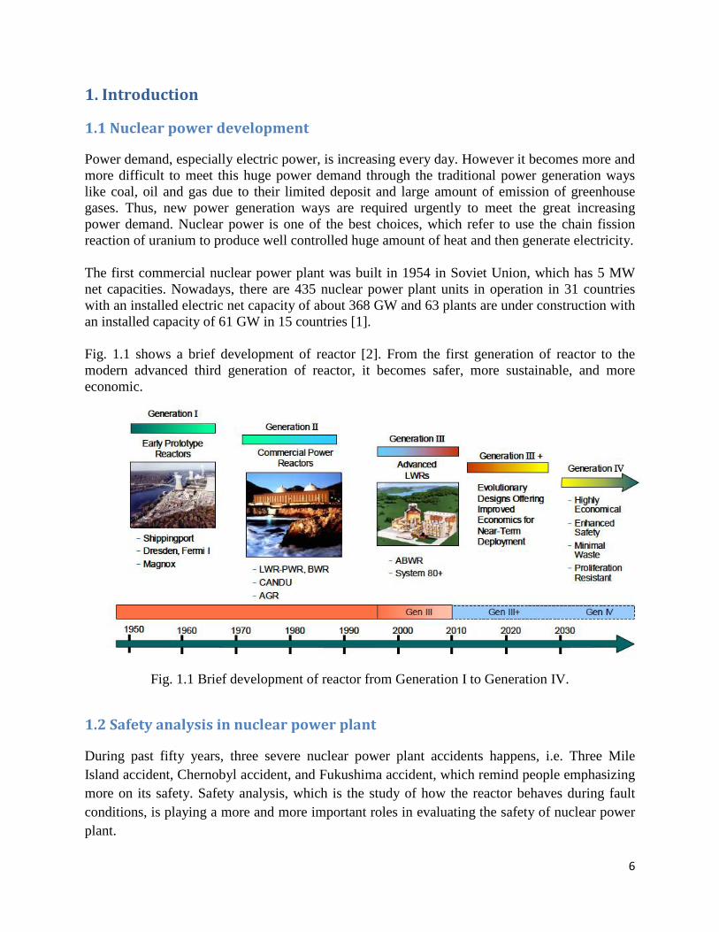
Power demand, especially electric power, is increasing every day. However it becomes more and more difficult to meet this huge power demand through the traditional power generation ways like coal, oil and gas due to their limited deposit and large amount of emission of greenhouse gases. Thus, new power generation ways are required urgently to meet the great increasing power demand. Nuclear power is one of the best choices, which refer to use the chain fission reaction of uranium to produce well controlled huge amount of heat and then generate electricity. The first commercial nuclear power plant was built in 1954 in Soviet Union, which has 5 MW net capacities. Nowadays, there are 435 nuclear power plant units in operation in 31 countries with an installed electric net capacity of about 368 GW and 63 plants are under construction with an installed capacity of 61 GW in 15 countries [1]. Fig. 1.1 shows a brief development of reactor [2]. From the first generation of reactor to the modern advanced third generation of reactor, it becomes safer, more sustainable, and more economic.

Fig. 1.1 Brief development of reactor from Generation I to Generation IV.

1.2 Safety analysis in nuclear power plant

During past fifty years, three severe nuclear power plant accidents happens, i.e. Three Mile Island accident, Chernobyl accident, and Fukushima accident, which remind people emphasizing more on its safety. Safety analysis, which is the study of how the reactor behaves during fault conditions, is playing a more and more important roles in evaluating the safety of nuclear power plant.

7

This thesis focuses on one of the design based accidents----Loss-Of-Coolant Accident (LOCA). Design based accident refers to a special category of events which are not expected to occur during the life time of the reactor but are presumed as a basis for design of the safety system. The LOCA can be categorized by the break occurring above and below the core as well as large and small break. In this work, all the three LOCA cases studied occur below the core with different break sizes. During large LOCA, shortly after the break, the coolant flow reverses in the core and dryout occurs within 2 seconds. After a short time, rewetting is caused by the downward two-phase flow which is generated by boiling of the water in the gaps between the coolant channels. During small and medium LOCA, the break flow leads to reactor scram and opening of pressure relief valve. The water level in the reactor vessel could fail down if the auxiliary feed water system cannot compensate for the break flow and for the steam generated by the residual heat [3].

Deterministic safety analysis is an important safety analysis method which helps to study the transient thermal-hydraulic behaviors when LOCA occurs through using calculation models to investigate the essential variables after the initial events. The purpose is to verify the safety design and to check whether licensing requirements are met [3]. Some computational codes have been developed to verify the design, licensing and safety of nuclear power plant. However, computational models are only approximation of the reality. Thus, validation of accuracy of computational codes becomes significantly important. Their validity should be tested against the realistic experimental results. In this thesis, The TRACE code (version 5.0 patch 2) is tested again FIX-II experiments. The aim is to simulate and understand the thermal-hydraulic behaviors when LOCA occurs in the primary system and validate of the TRACE code.

1.3 FIX-II program

The FIX-II experiments were performed in Sweden in 1980s by Studsvik Energiteknik AB in cooperation with AB Asea-Atom, which aim to produce an experimental data for understanding the initial stage of LOCA which is caused by a break in the main circulation line in Swedish BWRs and so as to verify the computational codes such as RELEP5 and TRACE. The purposes of FIX-II program can be briefly summarized as:

a. Determine the time for occurrence of the dryout in an electrically heated fuel rod bundle during loss of coolant accident.

b. Estimate the fuel rod temperature profile under different break sizes and different initial conditions, and calculate the corresponding heat transfer coefficient.

The test facility is based on Oskarshamn 2 which contains 444 fuel rod assemblies. Each assembly has 64 rods, and among them, 63 rods are powered. The volumetric scaling and power scaling between FIX-II and Oskarshamn 2 are 1:777 as shown in Equation (1-1). .

8

𝑉𝐹𝐼𝑋𝑉𝑂2

= 𝑃𝐹𝐼𝑋𝑃𝑂2

= 36444∗63

= 1777

(1-1)

The project plan can be summarized as 5 stages.

Stage 1: Reactor analysis of LOCA case for Oskarshamn 2 and scaling calculations were performed with reference to Oskarshamn 2 as model. Fuel rod simulators were developed.

Stage 2: Modification of FIX loop according to the results obtained in stage 1. Data collecting instrument was installed with corresponding computer program.

Stage 3: Running and trimming of experimental instrument.

Stage 4: Experimental stage includes 15 static dryout measurements, 7 LOCA and 6 - 8 pump trip experiments.

Stage 5: Experimental stage with additional LOCA and pump trip experiments. (General report part one) [4].

The cases studied in this thesis are experiments from stage 4 and 5.

1.4 TRACE code and SNAP

The TRAC/RELAP Advanced Computational Engine is developed by U.S. Nuclear Regulatory Commission (NRC) for analyzing transient and steady state thermal-hydraulic behavior in light water reactor. It is the product of combining NRC’s four main codes (TRAC-P, TRAC-B, RELAP5 and RAMONA) into one modernized computational code.

TRACE has been designed to perform the best-estimate analysis and prediction of thermal-hydraulic behavior in loss of coolant accidents, operational transients, and other accident scenarios in pressurized water reactors (PWRs), boiling water reactors (BWRs) and experimental facilities designed to simulate realistic reactors.

The Symbolic Nuclear Analysis Package (SNAP) is designed to simplify the process of performing thermal-hydraulic analysis. SNAP uses symbolic way to generate the input file, such as ASC II file for TRACE. It also allows the interaction between different codes. Currently, SNAP supports the RELAP5, TRACE, CONTAIN and FRAPCON-3 analysis codes. Support for the MELCOR AND FRAPTRAN codes is still under development [5].

TRACE uses a component-based approach to simulate a reactor system. Each component can represent a corresponding realistic component in the reactor system. The compromised hydraulic components generated by SNAP in TRACE used in this thesis are summarized in Table 1.1. In addition, the basic control blocks generated by SNAP are shown in Table 1.2 [6].

9

Table 1.1 The compromised hydraulic components used in this thesis.

Component name Function & Application Symbol

BREAK Component Apply the desired coolant flow

and pressure boundary conditions.

FILL Component Impose desired coolant flow rate and boundary condition

PIPE Component Models coolant flow in a 1D tube, channel, or pipe.

POWER Component

As a mean for delivering energy to fluid through HTSTR or hydraulic

component walls

PUMP Component Describe the interaction of the system fluid with a centrifugal

pump

HTSTR Component

Evaluate the dynamics of conduction, convection, and

gap-gas radiation heat transfer in a fuel-rod or structure

hardware component

VALVE Component Model various types of valves

associated with light water reactor.

Table 1.2 The basic control blocks used in this thesis.

Control system Function

Control blocks Function operators that operate on input signals to determine an output signal.

Trips

To decide when to evaluate a component hardware action. To define a ± 1.0 or 0.0 (ON or OFF) status signal for application

within a control block. To define a blocking or coincidence trip.

Signal variables The only means by which information is communicated to the control system.

The basic theory behind TRACE is the fluid field equations which model two-phase flow and the numerical approximations for solving these equations. Mass, energy, and momentum

10

conservation equations for the liquid and gas field compromise the basic two-fluid, two-phase field equation set, which gives rise to six partial differential equations to model two-phase flow. In addition, a series of approximations may also be needed to complete the closure of these field equations.

TRACE assumes that both liquid phase and gas phase have the same velocity and temperature. As a result, only one energy conservation equation and one momentum conservation equation are needed.

The six field conservation equations combined with interface jump condition can be expressed as the following equations [7].

Time Averaged Mass Equations:

𝜕[(1−𝛼)]𝜌𝑙���𝜕𝑡

+ 𝛻 �(1− 𝛼)𝜌𝑙�𝑉𝑙���⃗� � = −𝛤� (1-2)

𝜕�𝛼𝜌𝑔�����𝜕𝑡

+ ∇ �𝛼𝜌𝑔���𝑉𝑔���⃗� � = Γ� (1-3)

Time Average Energy Equations:

𝜕 �(1 − 𝛼)𝜌𝑙� �𝑒𝑙 + 𝑉𝑙22�

��������������

𝜕𝑡+ 𝛻 �(1 − 𝛼)𝜌𝑙� �𝑒𝑙 + 𝑉𝑙2

2� �𝑉𝑙���⃗�������������������

�

= −∇�(1− 𝛼)𝑞𝑙,����⃗ � + ∇ �(1 − 𝛼) �𝑇𝑙𝑉�⃗ 𝑙

������� + (1 − 𝛼)𝜌𝑙� �⃗�𝑉𝑙���⃗����� − 𝐸𝚤� + 𝑞𝑑𝑙���� (1-4)

𝜕 �𝛼𝜌𝑔��� �𝑒𝑔 + 𝑉𝑔22�

���������������

𝜕𝑡+ ∇ �𝛼𝜌𝑔��� �𝑒𝑔 + 𝑉𝑔2

2� �𝑉𝑔���⃗�������������������

�

= −∇�𝛼𝑞𝑔,�������⃗ � + ∇ �𝛼 �𝑇𝑔𝑉�⃗𝑔

�������� + 𝛼𝜌𝑔����⃗�𝑉𝑔���⃗����� − 𝐸𝚤� + 𝑞𝑑𝑔����� (1-5)

Time Average Momentum Equations:

𝜕�(1−𝛼)𝜌𝑙���𝑉𝑙����⃗����

𝜕𝑡+ ∇(1 − 𝛼)𝜌𝑙�𝑉𝑙���⃗ 𝑉𝑙���⃗

����� = ∇[(1 − 𝛼)𝑇𝑙� ] + (1 − 𝛼)𝜌𝑙� �⃗� − 𝑀𝚤��� (1-6)

𝜕�𝛼𝜌𝑔����𝑉𝑔����⃗�����

𝜕𝑡+ ∇𝛼𝜌𝑔���𝑉𝑔���⃗ 𝑉𝑔���⃗

����� = ∇�𝛼𝑇𝑔� � + 𝛼𝜌𝑔����⃗� + 𝑀𝚤��� (1-7)

11

In these equations, an over bar represents a time average, α is the probability that a point is occupied by gas phase, and Г, Ei, and Mi represent the contribution of time averaged jump conditions to transfer of mass, energy and momentum respectively. Besides, q’ is conductive heat flux, qd is the heat flux by direct heating and T is the full stress tensor. The subscripts of “g” and “l” represent gas and liquid term respectively.

12

2. Description of FIX-II test facility

2.1 General description of test facility

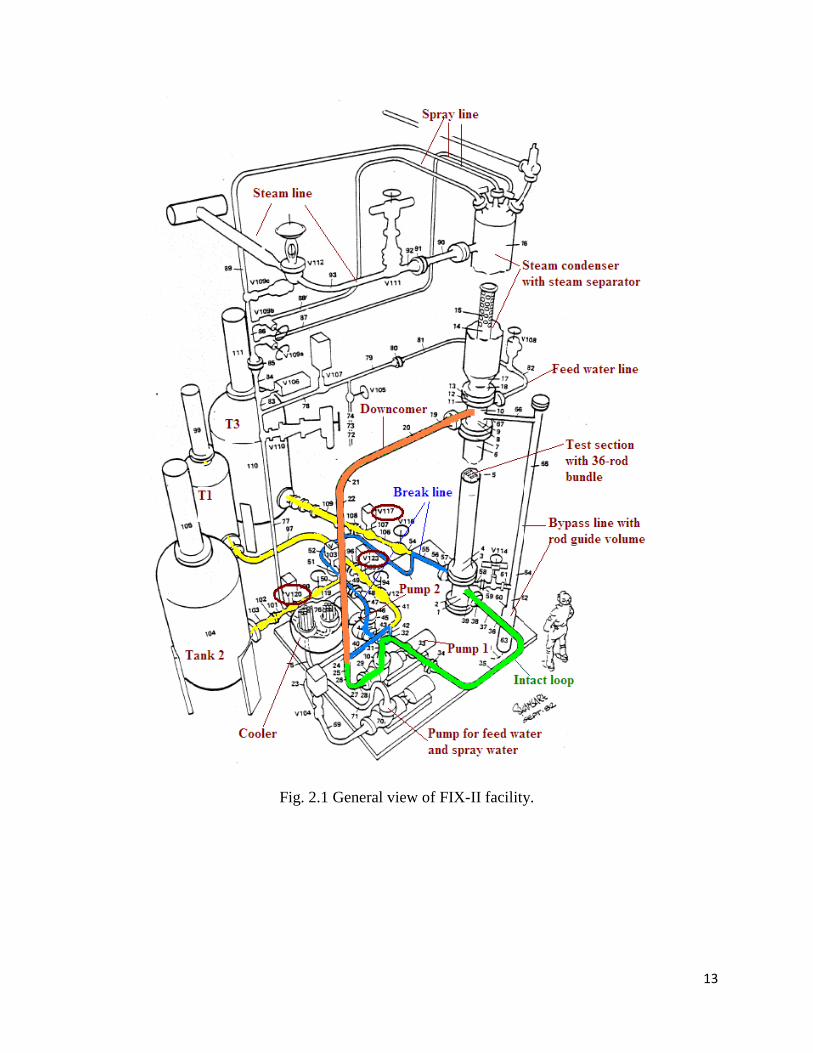
The test facility FIX-II is shown in Fig. 2.1. It contains the primary system and auxiliary system. In the primary system, the test section consists of a 36-rod bundle. A steam separator connects the test section with a spray condenser, where the steam generated from the test section will be condensed by the subcooled spray water from spray water line. After condensation, the condensed water mixes with the feed water and enters the downcomer. At the bottom of the downcomer, the water goes into three different lines: the break loop line where LOCA occurs, the intact loop line, and the cooling line which belongs to the auxiliary system. In the auxiliary system, the water is pumped from the downcomer to the cooling line and passes the tubes in evaporation cooler. Finally, it reaches the feed water line and spray line. Two pumps are used to deliver the water through the break loop line and intact loop line to the lower plenum which is connected with the test section and a bypass line. The bypass line is parallel with the test section and is heated by two electric rods. A rod guide tube is connected with the bypass line at the bottom, which simulates the control rod guide tube in the lower plenum and the moderate water. The water in the rod guide tube does not participate in the coolant circulation during steady state. The volume of main parts of the primary system compared with Oskarshamn 2 is stated in Table 2.1[4].

13

Fig. 2.1 General view of FIX-II facility.

14

Table 2.1 The volumetric scaling of FIX-II compared with Oskarshamn 2.

Part of primary system Oskarshamn 2 (m3) Ideally scaled FIX-II (dm3)

Actual FIX-II volume (dm3)

Lower plenum 34.8 44.8 30.6

Control rod guides in lower plenum 25.0 32.2 32.3

Bypass in core 23.3 30.0 32.8

Core inlet 1.1 1.4 0.8

Core 17.2 22.1 22.3

Core outlet 2.0 2.6 0.4

Upper plenum 8.1 10.4 7.6

Steam separator 11.3 14.5 16.7

Steam volume in steam dome 147 189 632

Downcomer, water at saturation temperature 29.5 38.0 39

Downcomer, subcooled part 60 77 77

Main recirculation lines, low side 10.2 13.1 25.4

Main recirculation lines, pressure side 23.1 29.9 53.3

2.2 Test section

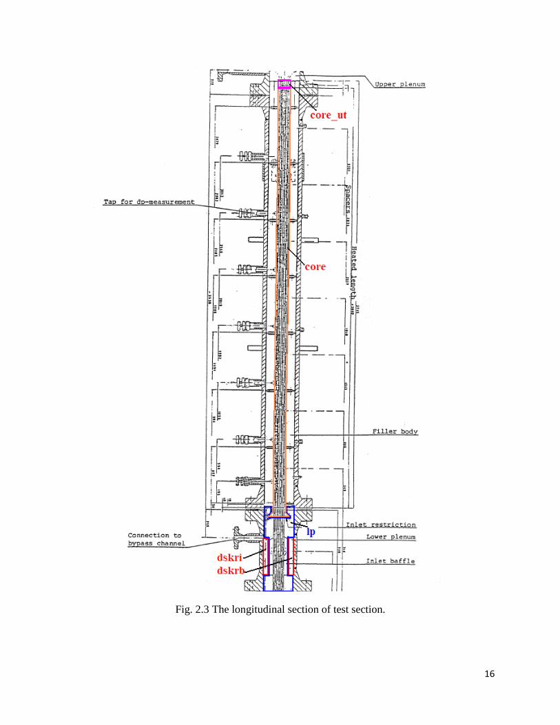
The test section consists of 36 electrical-heated rods with 3.68 m heating length, surrounded by a square canister fuel box which serves as a coolant channel. The cross section of the test section at heated part is shown in Fig. 2.2 and the longitudinal section is shown in Fig. 2.3. All the rods have the same diameter of 12.25 mm and the same separation of 16.3 mm. The square section where rods locate is supported by four reinforcement bars with inner radius of 101.8 mm and thickness of 2 mm. The geometrical arrangement gives the flow area of 6.03x10-3 m2 and the hydraulic diameter of 0.0136 m. The square section is surrounded by Teflon filler body as the thermal insulator. Between the pressure vessel and Teflon filler body, there is a gap filling water which will be heated during LOCA blowdown phase. The pressure vessel hangs in the flange coupling under the spray condenser. The inner radius of the pressure vessel is 264 mm and wall

15

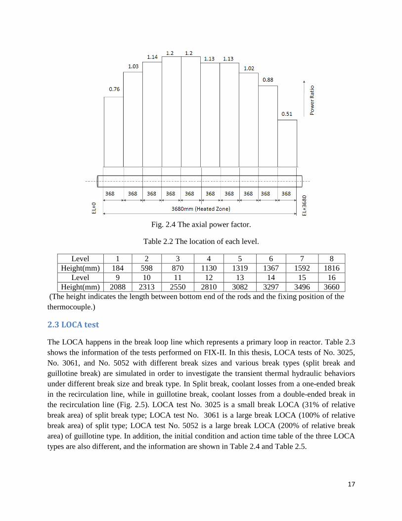
thickness is 30 mm. It contains a lower part (the lower plenum) which is 730 mm in height, a middle part which is 3630 mm in height, and an upper part (the upper plenum) which is also 730 mm in height. At the bottom, there is a plate where rods are bolted. The electrical power is used to directly heat the 36-rod bundle. The axial power distribution along the 36 rods is illustrated in Fig. 2.4. Along the rods, the thermocouples are fixed at 16 different longitudinal levels to monitor the temperature values of the rods. The location of each level is shown in Table 2.2[4].

(a)

(b)

Fig. 2.2 Test section: (a) the cross section of test section, (b) the cross section of the core: arrows indicate the detailed arrangement of thermocouples in the core.

16

Fig. 2.3 The longitudinal section of test section.

17

Fig. 2.4 The axial power factor.

Table 2.2 The location of each level.

Level 1 2 3 4 5 6 7 8 Height(mm) 184 598 870 1130 1319 1367 1592 1816

Level 9 10 11 12 13 14 15 16 Height(mm) 2088 2313 2550 2810 3082 3297 3496 3660

(The height indicates the length between bottom end of the rods and the fixing position of the thermocouple.)

2.3 LOCA test

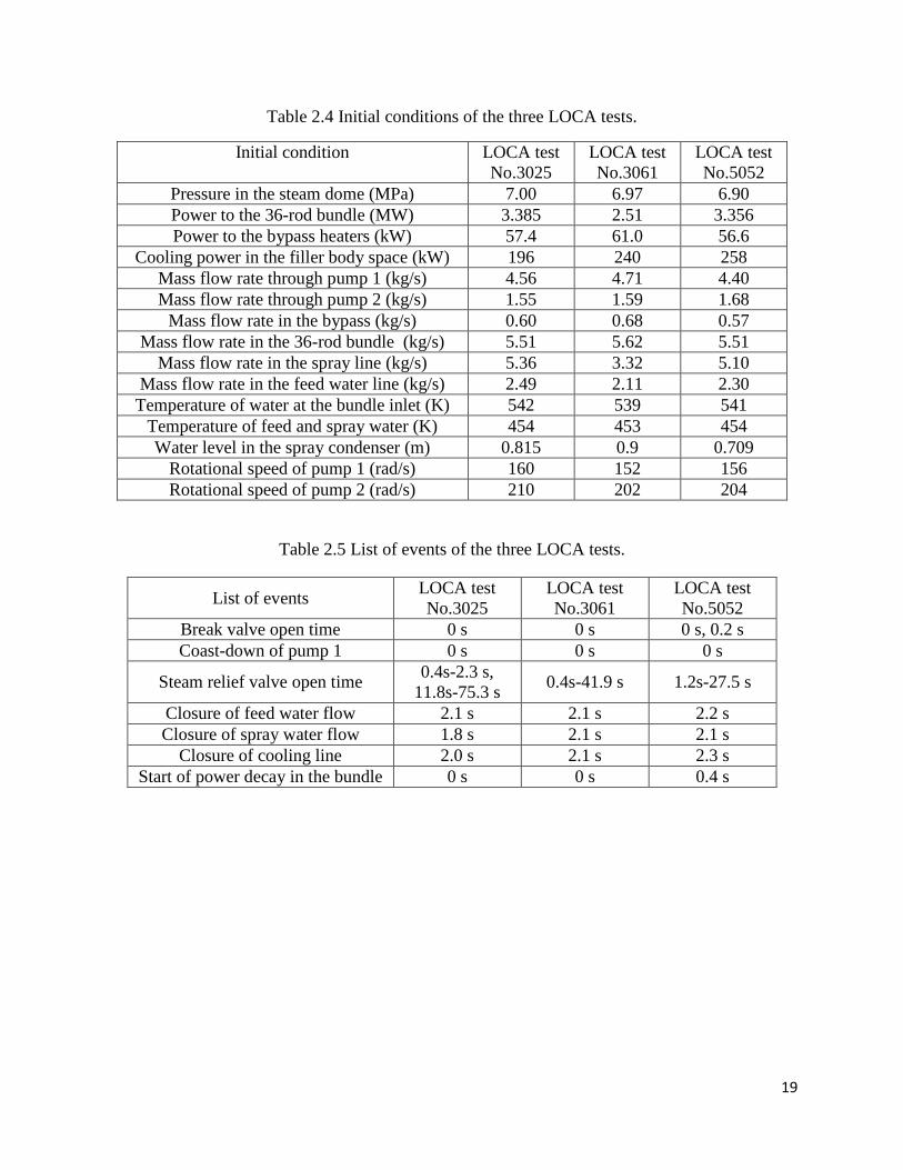
The LOCA happens in the break loop line which represents a primary loop in reactor. Table 2.3 shows the information of the tests performed on FIX-II. In this thesis, LOCA tests of No. 3025, No. 3061, and No. 5052 with different break sizes and various break types (split break and guillotine break) are simulated in order to investigate the transient thermal hydraulic behaviors under different break size and break type. In Split break, coolant losses from a one-ended break in the recirculation line, while in guillotine break, coolant losses from a double-ended break in the recirculation line (Fig. 2.5). LOCA test No. 3025 is a small break LOCA (31% of relative break area) of split break type; LOCA test No. 3061 is a large break LOCA (100% of relative break area) of split type; LOCA test No. 5052 is a large break LOCA (200% of relative break area) of guillotine type. In addition, the initial condition and action time table of the three LOCA types are also different, and the information are shown in Table 2.4 and Table 2.5.

18

Table 2.3 LOCA tests information.

Break classification Split breaks Guillotine

Type of simulation (see Figure)

A B C

Relative break area (%)

10 31 48 100 150 200 155 200

Break I.D. (mm) 6.8 12.0 15.0 21.6 26.4 30.5 16.0+21.6 21.6+21.6

Initial bundle power (MW)

2.35 2.35 3.35 3.35 2.35 2.35 2.35 2.35 2.35 3.35

LOCA test identification No.

3051 3013 3024 3025 3026 3027

3031 3061 3071 3041 4011 5061 5051 5052

Fig.2.5 Types of break of each LOCA test.

19

Table 2.4 Initial conditions of the three LOCA tests.

Initial condition LOCA test No.3025

LOCA test No.3061

LOCA test No.5052

Pressure in the steam dome (MPa) 7.00 6.97 6.90 Power to the 36-rod bundle (MW) 3.385 2.51 3.356 Power to the bypass heaters (kW) 57.4 61.0 56.6

Cooling power in the filler body space (kW) 196 240 258 Mass flow rate through pump 1 (kg/s) 4.56 4.71 4.40 Mass flow rate through pump 2 (kg/s) 1.55 1.59 1.68

Mass flow rate in the bypass (kg/s) 0.60 0.68 0.57 Mass flow rate in the 36-rod bundle (kg/s) 5.51 5.62 5.51

Mass flow rate in the spray line (kg/s) 5.36 3.32 5.10 Mass flow rate in the feed water line (kg/s) 2.49 2.11 2.30

Temperature of water at the bundle inlet (K) 542 539 541 Temperature of feed and spray water (K) 454 453 454 Water level in the spray condenser (m) 0.815 0.9 0.709

Rotational speed of pump 1 (rad/s) 160 152 156 Rotational speed of pump 2 (rad/s) 210 202 204

Table 2.5 List of events of the three LOCA tests.

List of events LOCA test No.3025

LOCA test No.3061

LOCA test No.5052

Break valve open time 0 s 0 s 0 s, 0.2 s Coast-down of pump 1 0 s 0 s 0 s

Steam relief valve open time 0.4s-2.3 s, 11.8s-75.3 s 0.4s-41.9 s 1.2s-27.5 s

Closure of feed water flow 2.1 s 2.1 s 2.2 s Closure of spray water flow 1.8 s 2.1 s 2.1 s

Closure of cooling line 2.0 s 2.1 s 2.3 s Start of power decay in the bundle 0 s 0 s 0.4 s

20

3. TRACE model

3.1 General description of model

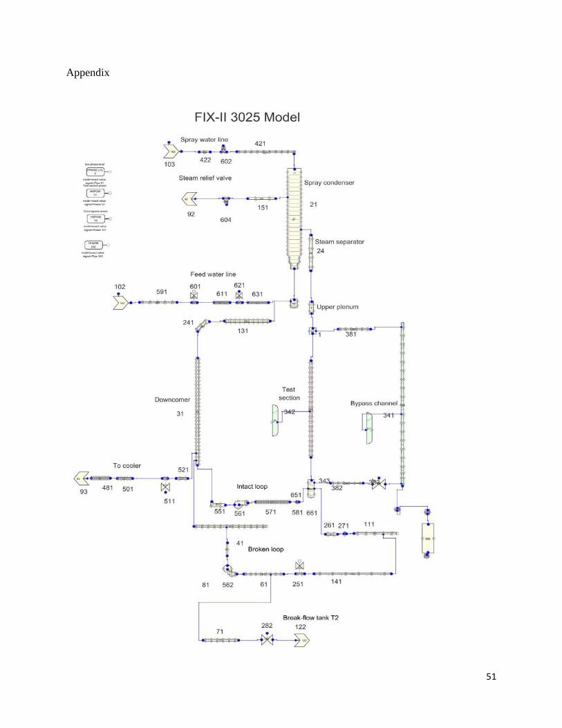
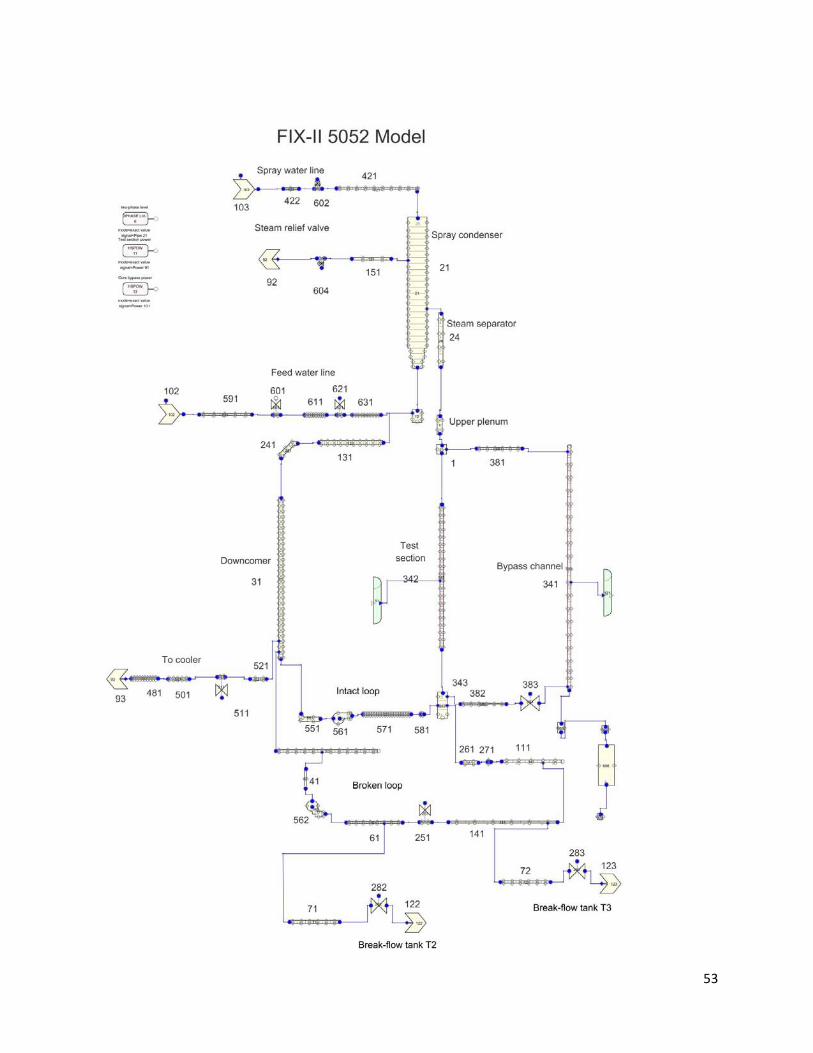
The model is generated by SNAP and the detail information is shown in Appendix. In the model, only the primary system is specifically simulated while the auxiliary system is replaced by one break component and two fill components so as to simplify the simulation model and realize the boundary conditions setting. The two fill components are used to represent the sub-cooled feed-water and spray water on the top of steam condenser respectively. The steam condenser is simulated by a pipe component, where steam is condensed by sub-cooled spray water. The test section is simulated by four pipe components (one for the core, another one for the lower plenum and the other two for upper plenum) and two heat structures. One of the heat structures has been used as the canister wall of the core, and the other heat structure has been used to simulate the fuel rod in the core. A power component is coupled to the heat structure which simulates the fuel rod in the core. The power distribution along the core is varied with experimental data. In addition to the test section, two pipes have been used to represent the downcomer and bypass which is also heated by a power-coupled heat structure. Two pump components are used to simulate the two main circulation pumps which force the coolant flow from downcomer to lower plenum. A valve component connected with a break component is used to represent the LOCA in the system. The desired break area is achieved by adjusting the valve flow area. The same principle is also applied in the steam relief valve.

The initial conditions of steady state are designed based on the parameters listed in Table 2.4. The first 1000 s is to present the steady state. After that, transient calculation is performed. During transient state, there are several valves need to be regulated according to the conditions shown in Table 2.5. The regulation of these valves is realized by a TRIP as illustrated in Fig. 3.1. The time variable during the transient is designed as illustrated in Fig. 3.2. In the Fig. 3.2, TIMEOF 10 is a signal of problem time. Control block -1 is a positive difference. Control block -3 is a sum of input of control block -1 and a constant -1000. The control black -3 can be used as the time variable during the transient.

(a)

21

(b)

Fig. 3.1 (a) Trip for valve regulation, (b) Logic of trip component.

(a)

(b)

Fig. 3.2 (a) time variable controlling logic, (b) Logic of control block -3

22

3.2 Improvement of the model

The model I start to work with is only a basic model which ignores the influence of some important physical items such as countercurrent flow limitation and choked flow. In order to better reflect the physical phenomena and validate the TRACE code based on the experimental results, several special physical models are applied into the simulations.

3.2.1 Countercurrent flow limitation (CCFL) model

Countercurrent flow limitation (CCFL) or flooding usually occurs when the vapor and liquid flow in the opposite direction. In the case of this work, the vapor goes upwards in the test section and upper plenum, while the liquid goes downwards due to the LOCA occurs at the bottom of the system during the transient state. When CCFL occurs, upwards vapor will limit the liquid flowing from the upper part of system to the lower part of the system. In present TRACE modeling, the CCFL model is employed since it will help to better predicting the liquid mass flow while avoid the over-prediction of downward liquid mass flow in the region of countercurrent flow [8].

In TRACE model, user can specify the correlations to evaluate CCFL. Three correlations are provided in TRACE code: Wallis, Kutateladze, and Bankoff. Wallis [9], Kutateladze [10], and Bankoff [11] correlations are as shown in following equations:

𝑗𝑔∗1/2 + 𝑚𝑤𝑗𝑓

∗1/2 = 𝐶𝑤 (3-1)

𝐾𝑔∗1/2 + 𝑚𝐾𝐾𝑓

1/2 = 𝐶𝐾 (3-2)

𝐻𝑔1/2 + 𝑚𝐵𝐻𝑓

1/2 = 𝐶𝐻 (3-3)

Where m and C are the constant determined by experimental data. 𝑗𝑖∗ ,𝐾𝑖∗ and 𝐻𝑖∗ are the dimensionless superficial velocity. The three correlations differ in their methods to determine the superficial velocity as below:

𝑗𝑖∗ = 𝑗𝑖 �𝜌𝑖

𝑔𝑑�𝜌𝑓−𝜌𝑔��1/2

(3-4)

𝐾𝐼 = 𝑗𝑖 �𝜌𝑖2

𝑔𝜎�𝜌𝑓−𝜌𝑔��1/2

(3-5)

𝐻𝑖∗ = 𝑗𝑖 �𝜌𝑖

𝑔𝑤�𝜌𝑓−𝜌𝑔��1/2

(3-6)

23

Where 𝑗𝑖 is the superficial velocity and 𝜌𝑖 is the density of phase i, 𝑑 is the diameter, 𝜎 is the surface tensor, and 𝑤 is the interpolative length scale determined from:

𝑤 = 𝑑1−𝛽𝐿1 𝛽 (0 ≤ 𝛽 ≤ 1) (3-7)

𝐿1 = � 𝜎𝑔�𝜌𝑓−𝜌𝑔�

�1/2

(3-8)

𝛽 = tanh(𝛾𝑘𝑐𝑑) (3-9)

𝑘𝑐 = 2𝜋𝑡𝑝

(3-10)

Where 𝐿1 is the Laplace capillary constant, 𝛽 is the scaling constant between 0 and 1, 𝑘𝑐 is the critical wave number, 𝛾 is the perforation ratio, and 𝑡𝑝 is the plate thickness.

In TRACE modeling, the occurrence location of CCFL and three parameters should be specified by users: (A) the interpolation constant, (B) the slope for the CCFL correlation and (C) the constant for the CCFL correlation. Previous studies [12] [13] show that Wallis correlation is more suitable for the pipe with small hydraulic diameter. In Wallis’s experiments, M is assumed from 0.8 to 1 and C is assumed from 0.7 to 1 for a vertical pipe. In present study, C is assumed 1 in all the cases, and M is 0.8 in case of 3025, while 1 in case of 3061 and 5052.

3.2.2 Choked-flow model

Choked flow, also named as critical flow, occurs when the mass flow rate in a pipe is independent from the downstream condition, which means the mass flow will remain constant even the downstream pressure changed. The choked flow occurs when the acoustic signals no longer influence the boundary condition which determines the mass flow rate at the choked plane [14]. Accurate prediction of such phenomenon has significant meaning in reactor safety simulation because the choked flow plays significant roles in how the reactor responds during such transient.

In the simulation model, the choked flow will occur in the break valve when the pressure difference is enormous. In TRACE NAMELIST variables DATA, two options are available for modeling the choked flow: default choked flow using default multiplier and user defined choked flow using optional multiplier. The second option is recommended because it has wilder application than the first option.

Choosing of appropriate choked-flow model by TRACE is based on void fraction. The choked flow in this study is a two phase flow, with the void fraction 1.0 × 10−5 < 𝛼 < 0.999 . As a result, a two phase choking calculation is done to predict choking velocity. The TRACE two-phase choked flow model calculation is based on the model developed by Ransom and Trapp

24

[15]. The optional multipliers will help to modify the calculated velocities through following two equations so as to improve the accuracy of prediction.

𝑉𝑚𝑒𝑝 = 𝛼𝑒𝜌𝑔𝑒𝑉𝑔𝑒+(1−𝛼𝑒)𝜌𝑙𝑒𝑉𝑙𝑒

𝜌𝑚𝑜 (3-11)

𝑉𝑙𝑒𝑝 = 𝐶𝐻𝑀𝐿𝑇2 ∙ 𝑉𝑚𝑒

𝑝 ∙𝜌𝑚𝑐𝜌𝑔𝑐𝛼𝑐𝑆+𝜌𝑙𝑐(1−𝛼𝑐)

(3-12)

Where 𝐶𝐻𝑀𝐿𝑇2 is a user-input choked-flow multiplier; 𝛼𝑒 is the cell-edge void fraction; 𝜌𝑙𝑒 and 𝜌𝑔𝑒 are the cell-edge saturation densities determined by the cell-edge pressure; 𝜌𝑔𝑐,𝜌𝑙𝑐, and 𝜌𝑚𝑐 are the cell-center steam/gas mixture, liquid and total mixture densities.

If the liquid velocity determined by the momentum solution is less than the maximum liquid choking velocity, the flow flag will be treated as non-choked flow and calculation will be ended. When the momentum calculated liquid velocity is equal or greater than the maximum choking velocity, the choked flow calculation will be performed and then liquid velocity will be set to the maximum liquid choking velocity. Besides, the gas/steam velocity is calculated in choked flow model as

𝑉𝑔𝑒𝑝 = 𝑆 ∙ 𝑉𝑙𝑒

𝑝 (3-13)

Where S is the slip ratio.

𝑆 = 𝑉𝑔𝑉𝑙

(3-14)

Where Vg and Vl are the momentum velocity solution for gas/steam and liquid respectively.

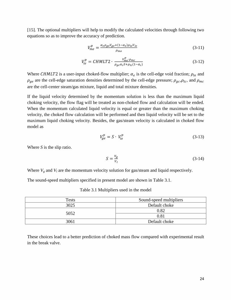
The sound-speed multipliers specified in present model are shown in Table 3.1.

Table 3.1 Multipliers used in the model

Tests Sound-speed multipliers 3025 Default choke

5052 0.82 0.81

3061 Default choke

These choices lead to a better prediction of choked mass flow compared with experimental result in the break valve.

25

3.2.3 Flow-area change loss calculation

Flow-area change loss and geometry of hydraulic component play a significant role in calculating the pressure drop profile and mass flow rate. Flow-area change results in change in the momentum flux term in the TRACE momentum equations. Flow-area change generally has four different scenarios: abrupt expansion, abrupt contraction, thin-plate-orifice, and pipe bending. The loss coefficients K for different scenarios are summarized in Table 3.2.

In namelist variables table, option of 1D reverse friction should be set to both forward and reverse because reverse flow will occur between the lower plenum and the break line during the transient state. The reverse flow may also occur in the test section and the bypass. A reverse K factor 1010 in TRACE model is applied to prevent the reverse flow from the auxiliary system to the primary system which does not occur in the experiment because of an existence of a pump in the cooling line. Lack of the reverse flow prevention will result in a little pressure increase which is inconsistent with experiment results. As a result, it has significant meaning to define the reverse friction in these components.

26

Table 3.2 K factor calculation in four scenarios [16] [17]

Abrupt expansion 𝐾 = �1 −

𝐴𝑗𝐴𝑗+1

�2

Abrupt contraction

𝐴𝑗+1𝐴𝑗

0.0 0.16 0.64 1.0

K 0.5 0.45 0.38 0.0

Thin-plate-orifice

𝐾 = �1 + 0.707�1 −Aj+1 2�

Aj

−Aj+1 2�

Aj�

2

Pipe bending

Small curvatures �𝑅𝑜𝐷ℎ

< 1.0� :

𝐾 = 0.0175 ∙ 𝜆 ∙ 𝑅𝑜𝐷ℎ∙ 𝛼 + 0.21

�𝑅𝑜𝐷ℎ�2.5 ∙ 𝐶

𝐶 = �0.9 ∙ sin𝛼 for 𝛼 ≤ 70°

1.0 for 𝛼 = 90°

0.7 + 0.35 ∙𝛼

90 for 𝛼 ≥ 90°

�

𝜆

= 𝑚𝑎𝑥 ��

64𝑅𝑒� , �

0.316𝑅𝑒0.25� ,

�2 log �𝐷ℎ

2 ∙ 𝑅𝑂𝑈𝐺𝐻�+ 1.74�

�

−2

Where Ro and Dh are the band radius and the hydraulic diameter of the pipe, respectively; 𝛼 is the bend angle; 𝜆 is the friction pressure loss coefficient.

Large curvatures �𝑅𝑜𝐷ℎ≥ 1.0� :

𝐾 = 0.0175 ∙ 𝜆 ∙ 𝑅𝑜𝐷ℎ∙ 𝛼 + 0.21

�𝑅𝑜𝐷ℎ�0.5 ∙ 𝐶

3.2.4 Pump modification

Two main circulation pumps are simulated in this model. During the steady state, the mass flow rate through each pump is evaluated by initial pump speed and rated values which includes rated head, rated torque, rated volumetric flow, rated density and rated speed. Correct input of initial pump speed value and rated values guarantee the desired mass flow.

27

During all the three LOCA tests, the coast-down of pump 1 in the intact recirculation line starts immediately after the break, and the power to pump 2 in the broken line is maintained. Correctly modeling coast-down of pump 1 has significant meaning for accurate prediction of rod temperature in the core. The impeller rotational speed of the pump is carefully designed to decease gradually in the transient state.

3.2.5 Break mass flow rate calculate

The break mass flow rate plays an important role in determining the transient behaviors like pressure drop and rod temperature patterns. It is necessary to guarantee the break mass flow in the simulation should be as much as that in experiment. Only ensuring this match, it is meaningful to analyze other transient behavior. In the experiment orifice flow meter has been used to measure the mass flow rate. However, the possibilities of evaluating two-phase mass flow from such measurements are limited, because void fraction and steam quality cannot be measured and the theoretical methods are imperfect. Fortunately the integrated value of the break flow mass is obtained with satisfactory accuracy from the water level increment in tanks T1-T3. The collecting tanks are filled with water. They are designed to serve both as condensation tanks for blown out steam and as measurement tanks for the integrated mass flow. If satisfactory condensation and no interference with non-condensable air, the level measurements should also give satisfactory information about the time sequence of the mass flow. As a result, the choked flow multiplier is designed to make the simulation result fitting to the integrated mass flow curve in the experimental data.

3.2.6 Geometry and initial conditions correctness

The geometry and initial conditions of each component are validated with the corresponding experimental configuration. The purpose of the validation is to make sure the correctness of fluid and steam distribution in the system. It also guarantees the total volume of the system which will influence the pressure drop ratio, fluid dynamic and heat transfer. Furthermore, correct initial conditions help the model to achieve the desired steady state.

3.2.7 Insulator in the steam dome

Activation of insulator option in the steam dome also has a significant influence on both steady state and transient state. During the steady state, the insulator has a similar function as the heat loss media which help the system to be condensed. While in the transient state, the temperature of insulator is higher than the system, so the insulator has inversed function of heating the steam dome to prevent the pressure dropping too fast.

28

4. Results and discussions

Based on FIX- II LOCA tests, simulation models for the tests of No. 3025, No. 3061 and No. 5052 were developed by using the TRACE code (version 5.0 patch 2) in present study. The main parameters during the tests are simulated, which are including the pressure, mass flow rate in some key parts (the break, the steam relief valve and the two circulation pumps), and temperature of both liquid and fuel rods in the fuel rod bundle. Consequently, The TRACE code is validated and qualified by comparison of these parameters between the experimental data and simulated results.

In all the three cases, the time 1000 s is chosen to coincide with the opening of the break valve which indicates the occurrence of break flow. The first 1000 s indicates the steady state situation. All the time shown in tables and text indicates the transient time which is corresponding to the opening of break valve.

4.1 LOCA test No. 3025

For the LOCA test of No. 3025, the break conditions are shown in Table 2.3 and Fig. 2.5, a split break amounting to 31 percent of the scaled down flow area of one recirculation pipe, combined with an initial bundle power of 3.38 MW. In this case, a relative small LOCA in split type is simulated. The purpose of the simulation is to see whether the TRACE model can reproduce the transient thermal-hydraulic behavior of a small LOCA in split type. The main results of TRACE simulation results including pressure, temperature at different locations and mass flow rate are summarized in Table 4.1 and Figs. 4.1-13. The corresponding experimental data are also plotted in the related figure for comparison.

Table 4.1 Comparison between experimental data and simulation results.

Experimental data Simulation results

Time of bundle uncover after break 49 s 51.5 s Maximum break mass flow rate 7.4 kg/s 7.46 kg/s Maximum mass flow through pump 1 6.6 kg/s 5.95 kg/s Maximum mass flow through pump 2 3.6 kg/s 3.6 kg/s Maximum dome pressure after the break 7.34 MPa 7.42 MPa Final dome pressure at the end of blowdown 2.15 MPa 2.08 MPa Maximum rod temperature 625 K 621 K Integrated break mass flow 214 kg 220.5 kg Integrated steam relief mass flow 39.7 kg 37.6 kg

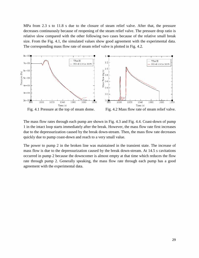
Fig. 4.1 shows the pressure transient at the top of steam dome when the break occurs. The pressure drops at the beginning of the transient because the opening of the steam relief valve and the closure of the spray and feed water. Then, the pressure goes up to a maximum value of 7.42

29

MPa from 2.3 s to 11.8 s due to the closure of steam relief valve. After that, the pressure decreases continuously because of reopening of the steam relief valve. The pressure drop ratio is relative slow compared with the other following two cases because of the relative small break size. From the Fig. 4.1, the simulated values show good agreement with the experimental data. The corresponding mass flow rate of steam relief valve is plotted in Fig. 4.2.

Fig. 4.1 Pressure at the top of steam dome. Fig. 4.2 Mass flow rate of steam relief valve.

The mass flow rates through each pump are shown in Fig. 4.3 and Fig. 4.4. Coast-down of pump 1 in the intact loop starts immediately after the break. However, the mass flow rate first increases due to the depressurization caused by the break down-stream. Then, the mass flow rate decreases quickly due to pump coast-down and reach to a very small value.

The power to pump 2 in the broken line was maintained in the transient state. The increase of mass flow is due to the depressurization caused by the break down-stream. At 14.5 s cavitations occurred in pump 2 because the downcomer is almost empty at that time which reduces the flow rate through pump 2. Generally speaking, the mass flow rate through each pump has a good agreement with the experimental data.

30

Fig. 4.3 Mass flow rate through pump 1 in the intact loop.

Fig. 4.4 Mass flow rate through pump 2 in the broken loop.

The mass flow rate through break is shown in Fig. 4.5 and the corresponding integrated mass flow rate is shown in Fig. 4.6. As mentioned in Section 3.2.5, it is impossible to measure the two-phase flow precisely under current technology. In order to guarantee the satisfied outcome, comparison of both break mass flow rate and integrated mass flow should be performed. A default choked flow model is applied in the break to well represent the experimental data. It can be found from the simulation that the maximum break flow rate is reached at the beginning, about 7.46 kg/s in the simulation, and 7.4 kg/s in the experimental data. The mass flow rate decreases after reaching the maximum value because of depressurization in the system which results in a reduced pressure difference in the break.

Fig. 4.5 Mass flow rate of the break. Fig. 4.6 Integrated mass flow of the break.

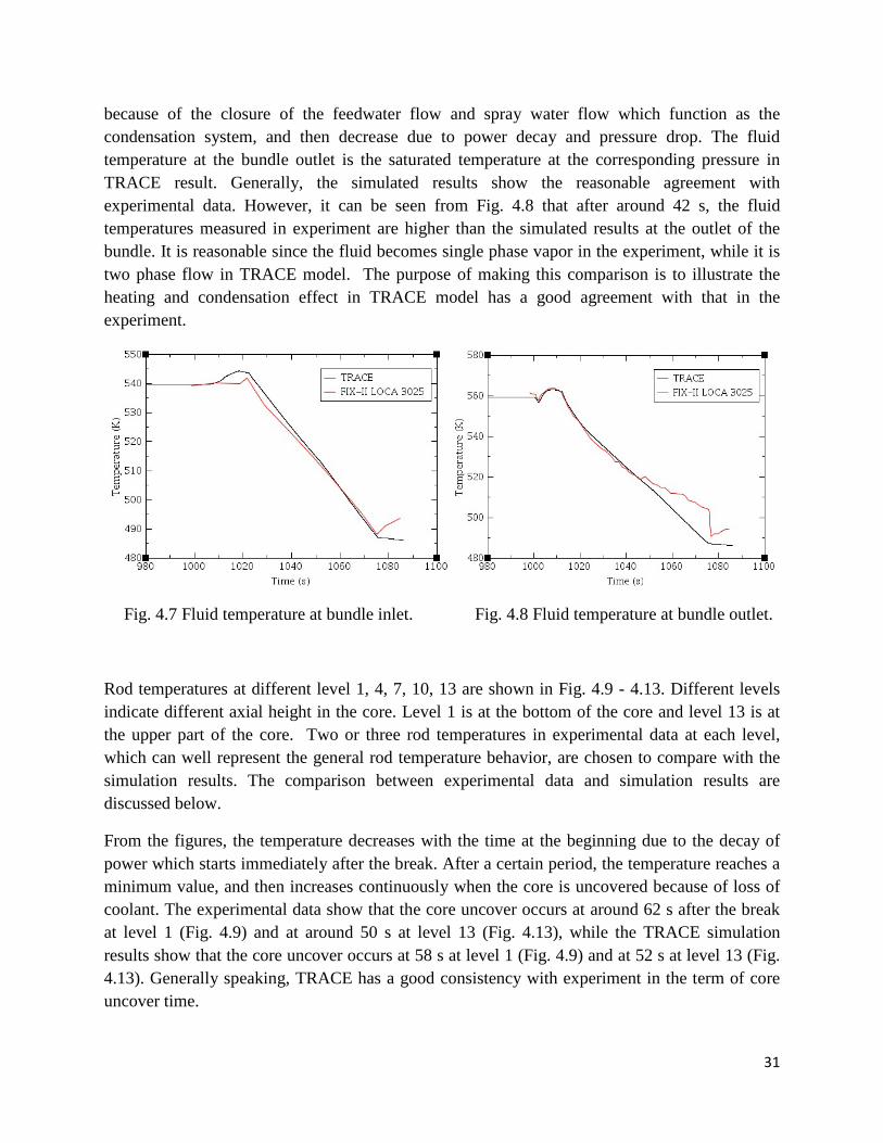
Fig. 4.7 and Fig. 4.8 illustrate the fluid temperature during the LOCA process at the inlet and outlet of the fuel rod bundle respectively. The Fluid temperature at the bundle inlet first increases

31

because of the closure of the feedwater flow and spray water flow which function as the condensation system, and then decrease due to power decay and pressure drop. The fluid temperature at the bundle outlet is the saturated temperature at the corresponding pressure in TRACE result. Generally, the simulated results show the reasonable agreement with experimental data. However, it can be seen from Fig. 4.8 that after around 42 s, the fluid temperatures measured in experiment are higher than the simulated results at the outlet of the bundle. It is reasonable since the fluid becomes single phase vapor in the experiment, while it is two phase flow in TRACE model. The purpose of making this comparison is to illustrate the heating and condensation effect in TRACE model has a good agreement with that in the experiment.

Fig. 4.7 Fluid temperature at bundle inlet. Fig. 4.8 Fluid temperature at bundle outlet.

Rod temperatures at different level 1, 4, 7, 10, 13 are shown in Fig. 4.9 - 4.13. Different levels indicate different axial height in the core. Level 1 is at the bottom of the core and level 13 is at the upper part of the core. Two or three rod temperatures in experimental data at each level, which can well represent the general rod temperature behavior, are chosen to compare with the simulation results. The comparison between experimental data and simulation results are discussed below.

From the figures, the temperature decreases with the time at the beginning due to the decay of power which starts immediately after the break. After a certain period, the temperature reaches a minimum value, and then increases continuously when the core is uncovered because of loss of coolant. The experimental data show that the core uncover occurs at around 62 s after the break at level 1 (Fig. 4.9) and at around 50 s at level 13 (Fig. 4.13), while the TRACE simulation results show that the core uncover occurs at 58 s at level 1 (Fig. 4.9) and at 52 s at level 13 (Fig. 4.13). Generally speaking, TRACE has a good consistency with experiment in the term of core uncover time.

32

There is a temperature sudden increase at the beginning of the transient which is considered as the occurrence of dryout. However, TRACE predicts differently with experiment result for the initial temperature increase. In the experiment, the dryout after the break is caused by the stagnation of the bundle flow and the initial depressurization and is quenched quickly because the steam relief valve and spray flow were closed, which lead to a pressure increase. The dryout is detected from level 11 and above in the experiment. However the simulation results by TRACE fails to predict the initial dryout, while predicts a core uncover from level 7 to level 13 (Fig. 4.11 - 4.13). In order to explain the difference, it is necessary to understand the principle for BWR dryout. The reason for a BWR dryout lies in the depressurization in the system. The depressurization will increase the void fraction and influence the mass flow rate in the fuel rod bundle, which contributes to the occurrence of dryout. The experiment date show that the dryout occurs at around 2 s after the depressurization; for simulation result, TRACE fails to predict the dryout while predicts a core uncover after that. It is probably because the dryout in the experiment is a local phenomenon, which only occurs in several rods not in all the rods. At the other hand, TRACE performs one-dimensional calculation which may result in the absence of the initial dryout. TRACE may also not predict the void distribution in the core very well leading to an occurrence of core uncover after that.

Fig. 4.9 Fuel rod temperature at level 1. Fig. 4.10 Fuel rod temperature at level 4.

Fig. 4.11 Fuel rod temperature at level 7. Fig. 4.12 Fuel rod temperature at level 10.

33

Fig. 4.13 Fuel rod temperature at level 13.

4.2 LOCA test No. 3061

For the test of No. 3061, the break conditions are shown in Table 2.3 and Fig. 2.5. In this case, a split break amounting to 100 percent of the scaled down flow area of one recirculation pipe, combined with an initial bundle power of 2.51 MW is simulated. The purpose of the simulation is to validate the TRACE model against a large LOCA in split type. The main results of experiment and TRACE simulation including pressure, temperature at different location and mass flow rate are summarized in Table 4.2 and illustrated in Figs. 4.14 - 4.27.

Table 4.2 Comparison between experimental data and simulation results

Experiment result TRACE result

Time to dryout after break 1.2 s 1.2 s Maximum break mass flow rate 19 kg/s 19.5 kg/s Maximum mass flow through pump 2 8 kg/s 8.4 kg/s Final dome pressure at the end of blowdown 2.02 MPa 2.05 MPa Maximum dryout temperature 887 K 822 K Maximum rod temperature at the end of the blowdown 804 K 795 K

Integrated break mass flow 268 kg 265.5 kg Integrated steam relief mass flow 14 kg 14.1 kg

Fig. 4.14 shows the pressure transient at the top of steam dome when the break occurs. The pressure at steam dome drops much rapidly than that in the small LOCA case. The pressure reaches the almost same value as the experimental data at the end of blow down phase. The mass

34

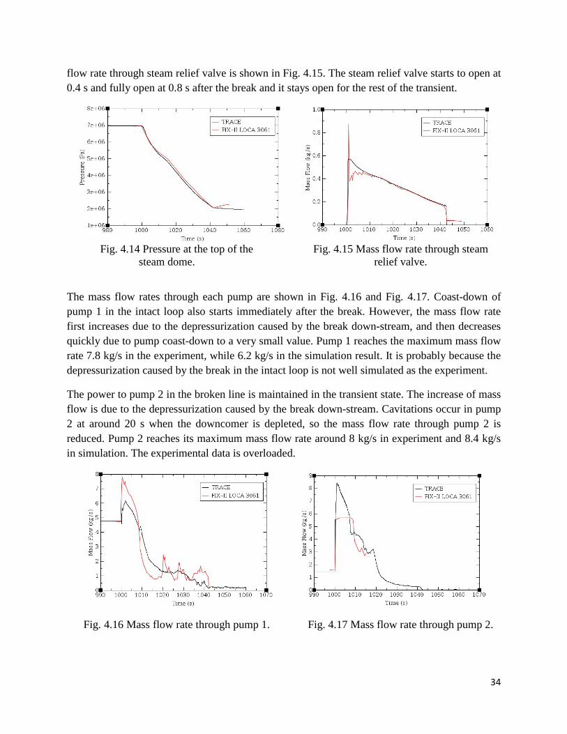
flow rate through steam relief valve is shown in Fig. 4.15. The steam relief valve starts to open at 0.4 s and fully open at 0.8 s after the break and it stays open for the rest of the transient.

Fig. 4.14 Pressure at the top of the

steam dome. Fig. 4.15 Mass flow rate through steam

relief valve.

The mass flow rates through each pump are shown in Fig. 4.16 and Fig. 4.17. Coast-down of pump 1 in the intact loop also starts immediately after the break. However, the mass flow rate first increases due to the depressurization caused by the break down-stream, and then decreases quickly due to pump coast-down to a very small value. Pump 1 reaches the maximum mass flow rate 7.8 kg/s in the experiment, while 6.2 kg/s in the simulation result. It is probably because the depressurization caused by the break in the intact loop is not well simulated as the experiment.

The power to pump 2 in the broken line is maintained in the transient state. The increase of mass flow is due to the depressurization caused by the break down-stream. Cavitations occur in pump 2 at around 20 s when the downcomer is depleted, so the mass flow rate through pump 2 is reduced. Pump 2 reaches its maximum mass flow rate around 8 kg/s in experiment and 8.4 kg/s in simulation. The experimental data is overloaded.

Fig. 4.16 Mass flow rate through pump 1. Fig. 4.17 Mass flow rate through pump 2.

35

The mass flow rate through break is shown in Fig. 4.18 and the corresponding integrated mass flow is shown in Fig. 4.19. A default choked flow model is also applied in the break to have a reasonable result with the experimental data. The maximum break flow of about 19 kg/s is reached in the experiment, and 19.4 kg/s in simulation. The mass flow rate decreases after reaching the maximum value because of depressurization in the system which results in a reduced pressure difference in the break. Fig. 4.18 and Fig. 4.19 show that the simulation results have a good agreement with experiment data.

Fig. 4.18 Mass flow rate through break. Fig. 4.19 Integrated mass flow through break.

Fig. 4.20 and Fig. 4.21 illustrate the fluid temperature development during the LOCA process at the inlet and outlet of the fuel rod bundle respectively. Generally, the simulated results show the reasonable agreement with experimental data. The fluid temperature at the bundle inlet first increases because the feedwater flow and spray flow are closed, which have the function of condensation system, and then decrease due to pressure drop and power decay. The purpose of making this comparison is to illustrate the heating and condensation effect in TRACE model has a good agreement with that in the experiment.

Fig. 4.20 Fluid temperature at bundle inlet.

Fig. 4.21 Fluid temperature at bundle outlet.

36

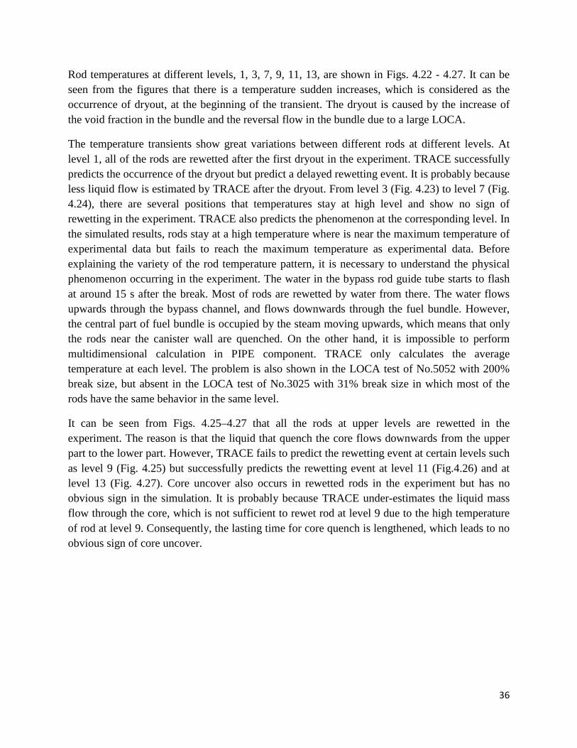
Rod temperatures at different levels, 1, 3, 7, 9, 11, 13, are shown in Figs. 4.22 - 4.27. It can be seen from the figures that there is a temperature sudden increases, which is considered as the occurrence of dryout, at the beginning of the transient. The dryout is caused by the increase of the void fraction in the bundle and the reversal flow in the bundle due to a large LOCA.

The temperature transients show great variations between different rods at different levels. At level 1, all of the rods are rewetted after the first dryout in the experiment. TRACE successfully predicts the occurrence of the dryout but predict a delayed rewetting event. It is probably because less liquid flow is estimated by TRACE after the dryout. From level 3 (Fig. 4.23) to level 7 (Fig. 4.24), there are several positions that temperatures stay at high level and show no sign of rewetting in the experiment. TRACE also predicts the phenomenon at the corresponding level. In the simulated results, rods stay at a high temperature where is near the maximum temperature of experimental data but fails to reach the maximum temperature as experimental data. Before explaining the variety of the rod temperature pattern, it is necessary to understand the physical phenomenon occurring in the experiment. The water in the bypass rod guide tube starts to flash at around 15 s after the break. Most of rods are rewetted by water from there. The water flows upwards through the bypass channel, and flows downwards through the fuel bundle. However, the central part of fuel bundle is occupied by the steam moving upwards, which means that only the rods near the canister wall are quenched. On the other hand, it is impossible to perform multidimensional calculation in PIPE component. TRACE only calculates the average temperature at each level. The problem is also shown in the LOCA test of No.5052 with 200% break size, but absent in the LOCA test of No.3025 with 31% break size in which most of the rods have the same behavior in the same level.

It can be seen from Figs. 4.25–4.27 that all the rods at upper levels are rewetted in the experiment. The reason is that the liquid that quench the core flows downwards from the upper part to the lower part. However, TRACE fails to predict the rewetting event at certain levels such as level 9 (Fig. 4.25) but successfully predicts the rewetting event at level 11 (Fig.4.26) and at level 13 (Fig. 4.27). Core uncover also occurs in rewetted rods in the experiment but has no obvious sign in the simulation. It is probably because TRACE under-estimates the liquid mass flow through the core, which is not sufficient to rewet rod at level 9 due to the high temperature of rod at level 9. Consequently, the lasting time for core quench is lengthened, which leads to no obvious sign of core uncover.

37

Fig. 4.22 Rod temperature at level 1. Fig. 4.23 Rod temperature at level 3.

Fig. 4.24 Rod temperature at level 7. Fig. 4.25 Rod temperature at level 9.

Fig. 4.26 Rod temperature at level 11. Fig. 4.27 Rod temperature at level 13.

38

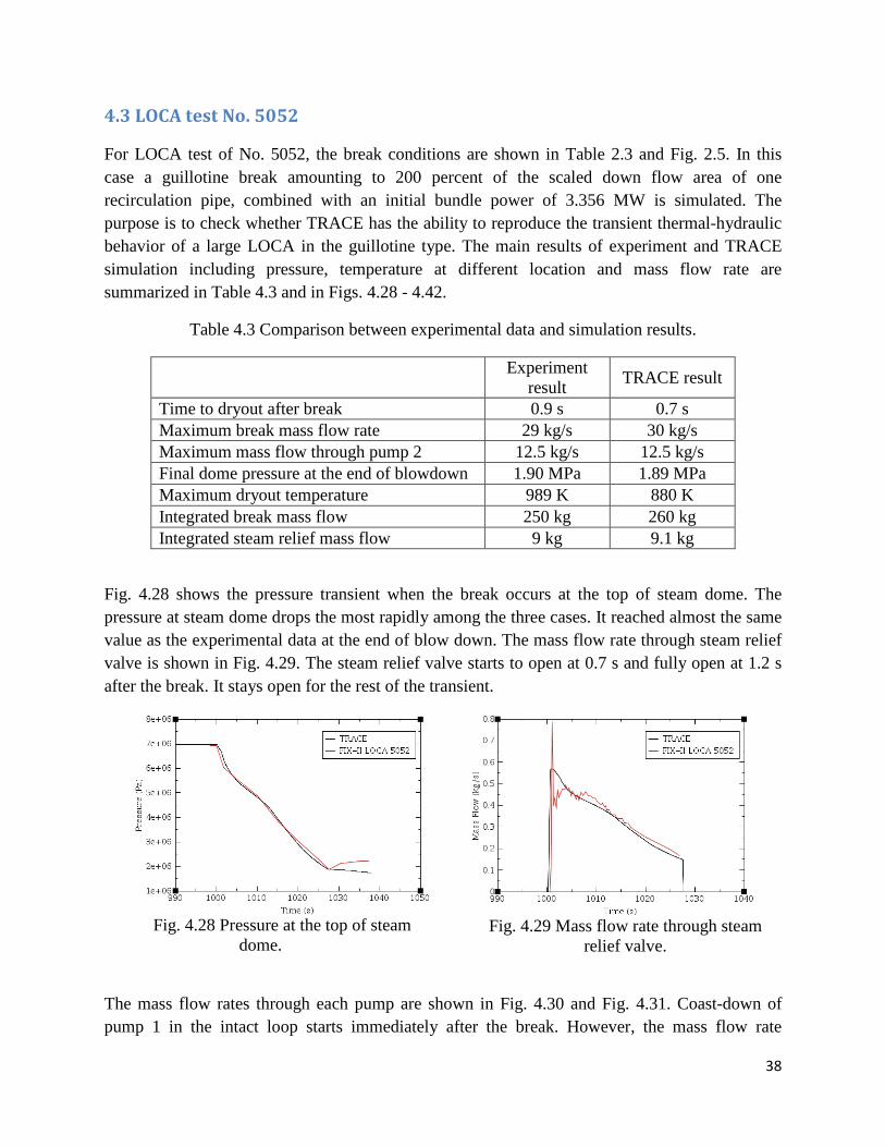
4.3 LOCA test No. 5052

For LOCA test of No. 5052, the break conditions are shown in Table 2.3 and Fig. 2.5. In this case a guillotine break amounting to 200 percent of the scaled down flow area of one recirculation pipe, combined with an initial bundle power of 3.356 MW is simulated. The purpose is to check whether TRACE has the ability to reproduce the transient thermal-hydraulic behavior of a large LOCA in the guillotine type. The main results of experiment and TRACE simulation including pressure, temperature at different location and mass flow rate are summarized in Table 4.3 and in Figs. 4.28 - 4.42.

Table 4.3 Comparison between experimental data and simulation results.

Experiment result TRACE result

Time to dryout after break 0.9 s 0.7 s Maximum break mass flow rate 29 kg/s 30 kg/s Maximum mass flow through pump 2 12.5 kg/s 12.5 kg/s Final dome pressure at the end of blowdown 1.90 MPa 1.89 MPa Maximum dryout temperature 989 K 880 K Integrated break mass flow 250 kg 260 kg Integrated steam relief mass flow 9 kg 9.1 kg

Fig. 4.28 shows the pressure transient when the break occurs at the top of steam dome. The pressure at steam dome drops the most rapidly among the three cases. It reached almost the same value as the experimental data at the end of blow down. The mass flow rate through steam relief valve is shown in Fig. 4.29. The steam relief valve starts to open at 0.7 s and fully open at 1.2 s after the break. It stays open for the rest of the transient.

Fig. 4.28 Pressure at the top of steam

dome. Fig. 4.29 Mass flow rate through steam

relief valve.

The mass flow rates through each pump are shown in Fig. 4.30 and Fig. 4.31. Coast-down of pump 1 in the intact loop starts immediately after the break. However, the mass flow rate

39

increases due to the depressurization caused by the break down-stream. The mass flow rate decreases quickly due to pump coast-down and reaches to a very small value.

The power to pump 2 in the broken line is maintained. The increase of mass flow is due to the depressurization caused by the break down-stream. Pump 2 reaches its maximum mass flow rate around 12.5 kg/s in experiment and 11.94 kg/s in simulation.

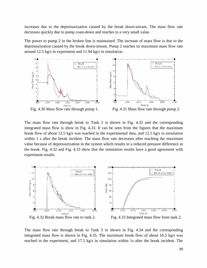
Fig. 4.30 Mass flow rate through pump 1. Fig. 4.31 Mass flow rate through pump 2.

The mass flow rate through break to Tank 2 is shown in Fig. 4.32 and the corresponding integrated mass flow is show in Fig. 4.33. It can be seen from the figures that the maximum break flow of about 12.5 kg/s was reached in the experimental data, and 12.5 kg/s in simulation within 1 s after the break incident. The mass flow rate decreases after reaching the maximum value because of depressurization in the system which results in a reduced pressure difference in the break. Fig. 4.32 and Fig. 4.33 show that the simulation results have a good agreement with experiment results.

Fig. 4.32 Break mass flow rate to tank 2. Fig. 4.33 Integrated mass flow from tank 2.

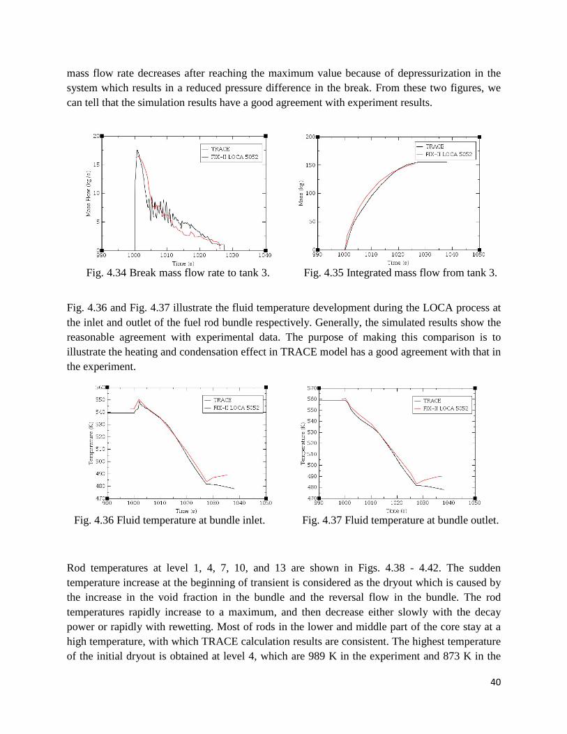
The mass flow rate through break to Tank 3 in shown in Fig. 4.34 and the corresponding integrated mass flow is shown in Fig. 4.35. The maximum break flow of about 16.5 kg/s was reached in the experiment, and 17.5 kg/s in simulation within 1s after the break incident. The

40

mass flow rate decreases after reaching the maximum value because of depressurization in the system which results in a reduced pressure difference in the break. From these two figures, we can tell that the simulation results have a good agreement with experiment results.

Fig. 4.34 Break mass flow rate to tank 3. Fig. 4.35 Integrated mass flow from tank 3.

Fig. 4.36 and Fig. 4.37 illustrate the fluid temperature development during the LOCA process at the inlet and outlet of the fuel rod bundle respectively. Generally, the simulated results show the reasonable agreement with experimental data. The purpose of making this comparison is to illustrate the heating and condensation effect in TRACE model has a good agreement with that in the experiment.

Fig. 4.36 Fluid temperature at bundle inlet. Fig. 4.37 Fluid temperature at bundle outlet.

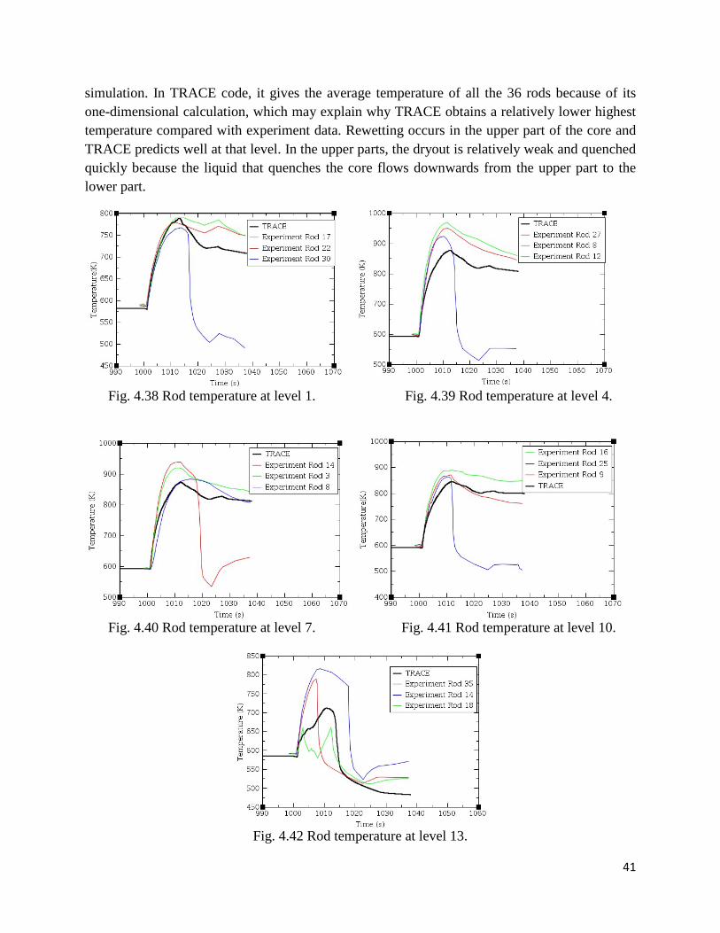
Rod temperatures at level 1, 4, 7, 10, and 13 are shown in Figs. 4.38 - 4.42. The sudden temperature increase at the beginning of transient is considered as the dryout which is caused by the increase in the void fraction in the bundle and the reversal flow in the bundle. The rod temperatures rapidly increase to a maximum, and then decrease either slowly with the decay power or rapidly with rewetting. Most of rods in the lower and middle part of the core stay at a high temperature, with which TRACE calculation results are consistent. The highest temperature of the initial dryout is obtained at level 4, which are 989 K in the experiment and 873 K in the

41

simulation. In TRACE code, it gives the average temperature of all the 36 rods because of its one-dimensional calculation, which may explain why TRACE obtains a relatively lower highest temperature compared with experiment data. Rewetting occurs in the upper part of the core and TRACE predicts well at that level. In the upper parts, the dryout is relatively weak and quenched quickly because the liquid that quenches the core flows downwards from the upper part to the lower part.

Fig. 4.38 Rod temperature at level 1. Fig. 4.39 Rod temperature at level 4.

Fig. 4.40 Rod temperature at level 7. Fig. 4.41 Rod temperature at level 10.

Fig. 4.42 Rod temperature at level 13.

42

4.4 Sensitivity analysis

TRACE model is defined by a serial of equations, parameters, and variables. Sensitivity analysis is the study of how and to what extent an input of a model can influence the output of a model. Sensitivity Analysis has the ability of sequencing by significance the strength and relevance of the inputs in determining the variation in the output [18]. It is essential to perform the sensitivity analysis after computational simulation. In this thesis, some physical model and input parameters, which are considered potentially to have the most significant influence upon the model and play an great important role in the correctness of TRACE modeling, are chosen including CCFL model, choked flow model, insulator in the steam condenser, K-factor in test section and pump trip.

4.4.1 CCFL model

Countercurrent flow is a very common phenomenon in BWR, and occurs at the top of the core and bundle inlet orifice. If countercurrent flow limitation (CCFL) occurs, the upwards vapor will limit the liquid flowing from the upper part of the system to the lower part of the system, which will cause the sudden increase of rod temperature in the core. Properly considering the influence of CCFL model upon the core is quite significant, and will lead to a more precise prediction of liquid mass flow in the core. As a result, activation of CCFL model has significant meaning in the correctness of TRACE modeling. The purpose of performing this sensitivity study is to test the importance of CCFL model and to investigate the influence of the CCFL activation on the output. TRACE model of LOCA test of No. 3025 without activation of CCFL are compared against TRACE model with CCFL. Rod temperatures at level 1, 7, 10, and 14 are compared in Fig. 4.43 - 4.46. It can be seen from the figures that the CCFL model has less influence on the temperatures of the lower parts of the rods, but a significant influence upon the upper parts. The reason is that at the upper part of the rod, the vapor velocity and void fraction reach a larger value; it leads to a smaller liquid mass flow rate according to CCFL model correlation. In conclusion, absence of CCFL model will lead to an over-estimated rod rewetting, and the influence is quite significant.

43

Fig. 4.43 Comparison of models with and without CCFL model at rod level 1 in

LOCA test 3025.

Fig. 4.44 Comparison of models with and without CCFL model at rod level 7 in

LOCA test 3025.

Fig. 4.45 Comparison of models with and

without CCFL model at rod level 10 in LOCA test 3025.

Fig. 4.46 Comparison of rod temperature with and without CCFL model at level 13 in

LOCA test 3025.

4.4.2 Choked flow model

Choked flow, or critical flow, occurs in the break due to the huge pressure difference when opening of break valve. Accurate prediction of such phenomenon has significant meaning in reactor safety simulation because the choked flow plays important roles in how the reactor responds during transient. The activation of choked flow model in the break valve will lead to a more reasonable break mass flow rate. The amount of coolant lost in the break will directly determine the mass and energy balance of the whole system. As a result, the importance of choked flow model and its influence upon the outcome are investigated in the sensitivity study.

44

TRACE model of LOCA test of No. 5052 without choked flow model are compared against the model with choked flow model. The mass flow rates through break to tank 2 and 3 are shown in Fig. 4.47 and Fig. 4.48. Pressure at the top of steam dome is shown in Fig. 4.49. It is obvious to notice that absence of choked flow model will lead to an over-estimated mass flow rate (Fig. 4.47, Fig. 4.48) which caused the pressure to drop much faster than that in the experiment (Fig. 4.49). In conclusion, the choked flow model indeed leads to a better prediction of the break mass flow rate, and the influence is quite significant.

Fig. 4.47 The break mass flow rate to tank 2 calculated with and without activation of choked flow model in LOCA test 5052.

Fig. 4.48 The break mass flow rate to tank 3 calculated with and without activation of choked flow model in LOCA test 5052.

Fig. 4.49 Pressure in the steam dome with and without activation of choked flow model in LOCA test 5052.

4.4.3 Insulator in the steam dome

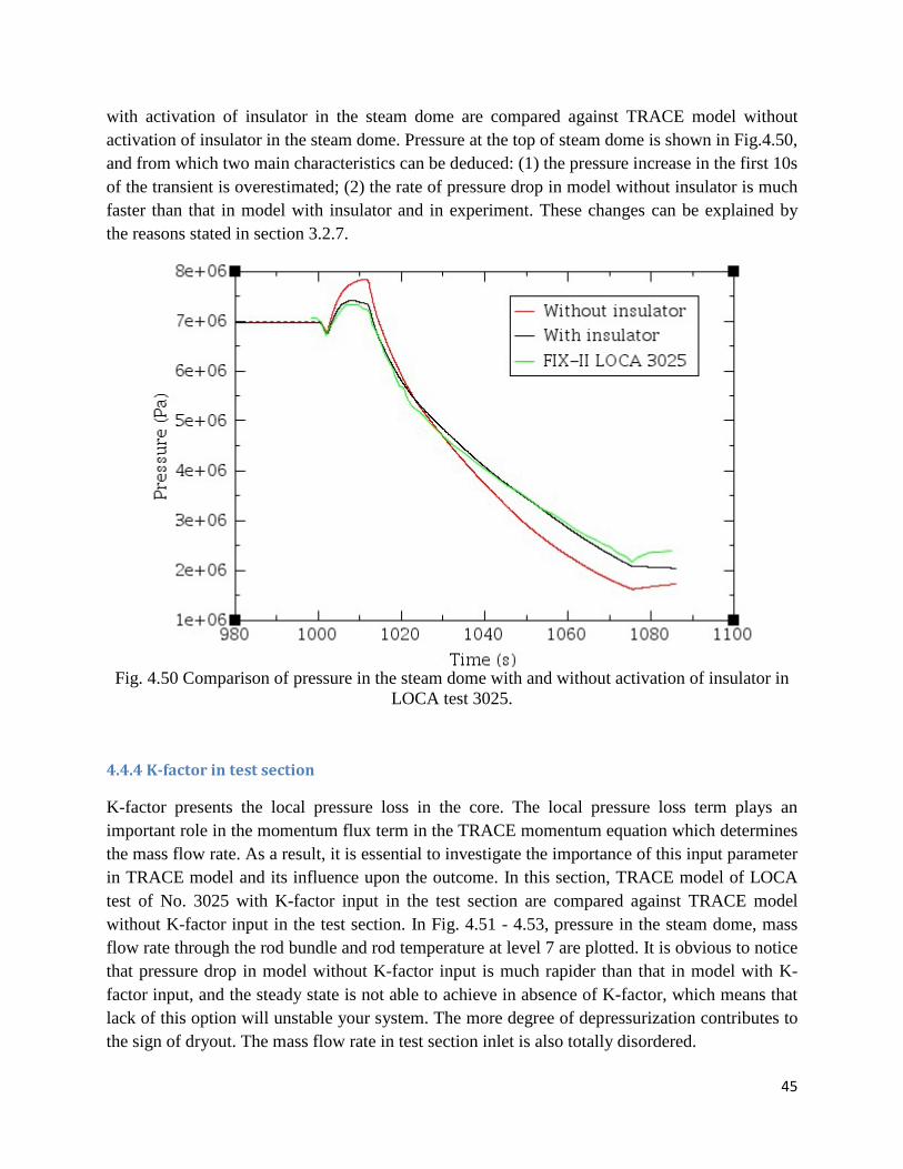
As mentioned in section 3.2.7, insulator is an important parameter in the term of energy balance. In order to verify the theory in section 3.2.7 and investigate the influence of the insulator upon the outcome, sensitivity analysis is performed. In this section, TRACE model of test of No. 3025

45

with activation of insulator in the steam dome are compared against TRACE model without activation of insulator in the steam dome. Pressure at the top of steam dome is shown in Fig.4.50, and from which two main characteristics can be deduced: (1) the pressure increase in the first 10s of the transient is overestimated; (2) the rate of pressure drop in model without insulator is much faster than that in model with insulator and in experiment. These changes can be explained by the reasons stated in section 3.2.7.

Fig. 4.50 Comparison of pressure in the steam dome with and without activation of insulator in

LOCA test 3025.

4.4.4 K-factor in test section

K-factor presents the local pressure loss in the core. The local pressure loss term plays an important role in the momentum flux term in the TRACE momentum equation which determines the mass flow rate. As a result, it is essential to investigate the importance of this input parameter in TRACE model and its influence upon the outcome. In this section, TRACE model of LOCA test of No. 3025 with K-factor input in the test section are compared against TRACE model without K-factor input in the test section. In Fig. 4.51 - 4.53, pressure in the steam dome, mass flow rate through the rod bundle and rod temperature at level 7 are plotted. It is obvious to notice that pressure drop in model without K-factor input is much rapider than that in model with K-factor input, and the steady state is not able to achieve in absence of K-factor, which means that lack of this option will unstable your system. The more degree of depressurization contributes to the sign of dryout. The mass flow rate in test section inlet is also totally disordered.

46

Fig. 4.51 Comparison of pressure in the

steam dome with and without K-factor in test section in LOCA test 3025.

Fig. 4.52 Comparison of liquid mass flow rate in the inlet of test section with and

without K-factor in test section in LOCA test 3025.

Fig. 4.53 Comparison of rod temperature at level 7 with and without K-factor in test section in

LOCA test 3025.

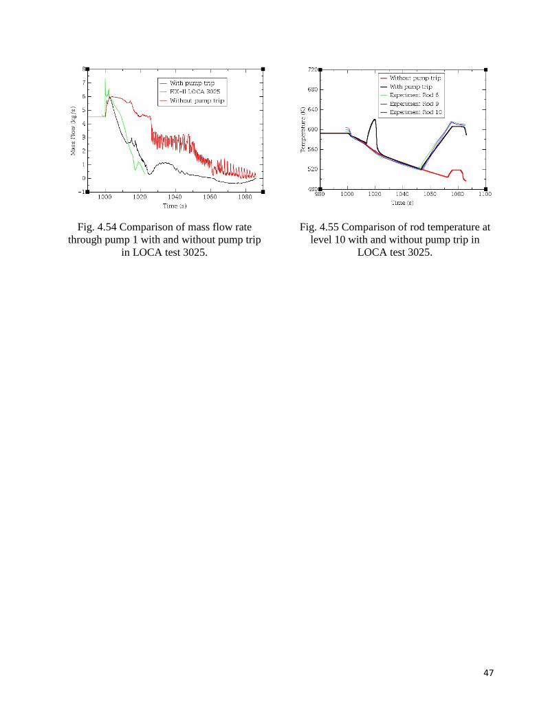
4.4.5 Pump trip in the intact loop

The pump trip in the intact loop is a quite important event in a LOCA transient in BWR. During a LOCA transient, the mass flow in the recirculation line will become unstable because of failure of power regulator. The increase of the mass flow in the recirculation line will lead to an increase of reactor power. Reduction of pump speed and hence a decrease in mass flow will result in an insignificant transient. The reactor power will be stabilized at a certain level corresponding to the lower pump speed. Pump coast-down should be initialed [3]. After pump coast-down, the coolant flow is reduced, which affects the core cooling condition. In order to investigate its influence upon the core cooling condition, sensitivity study is performed. In this section, TRACE models of LOCA test of No. 3025 with and without pump trip are compared in Fig. 4.54 and Fig. 4.55. It can be deduces from Fig. 4.55 that pump trip reduces the mass flow in the circulation line, and which do affect the core cooling condition.

47

Fig. 4.54 Comparison of mass flow rate through pump 1 with and without pump trip

in LOCA test 3025.

Fig. 4.55 Comparison of rod temperature at level 10 with and without pump trip in

LOCA test 3025.

48

5. Conclusions

Motivated by validation of TRACE code as well as trying to interpret the thermal-hydraulic behavior during loss-of-coolant accident in the primary system. TRACE simulation models are validated by comparing the simulation results against the FIX-II LOCA experiments of No. 3025, No. 3061 and No. 5052 in this thesis.

The simulated transient thermal-hydraulic behaviors during the LOCA tests including the pressure in the primary system, the mass flow rate in certain key parts, and the temperature in the core are compared with experimental data. Generally speaking, the simulation results have a good agreement with the experimental data for all the three cases studied, which means TRACE model has the ability to simulate the transient thermal-hydraulic behaviors under different break size. Furthermore, TRACE has a better performance on LOCA test No. 3025 than on LOCA test No. 3061 and No. 5052, which means that TRACE is more suitable to simulate the LOCA transient in a small break LOCA case. However, there are some differences between TRACE simulation results and experimental data, which will be discussed in the three tests respectively.

For the test of No. 3025 with 31% break size, the relative small break size only causes a minor dryout which indicated by the sharp peak at the beginning of the transient. It can be seen from the simulated temperature profile that there is a great difference between simulation results and the experimental data. TRACE fails to predict the initial dryout because it is a local phenomenon in the experiment, which can be omitted by the one-dimensional calculation of TRACE code. However, in the term of core uncover time, the simulated results have a good agreement with experimental data except level 1 in the bottom of fuel bundle.

For the test of No. 3061 with 100% break size, the relative large break size causes the immediately dryout within 2 s after the break which has a good agreement with experimental data. However, rewetting event of the rods predicted by TRACE has some inconsistency with the experimental data. TRACE fails to simulate the rewetting in certain levels like level 9, but successfully predicts the rewetting in upper levels like level 11 and level 13. Furthermore, TRACE also fails to predict core uncover in the rewetted rods compare to experimental data. It is probably because TRACE under-estimate the velocity of the liquid mass flow through the core, which results in insufficient rewetting at certain level. Consequently, the lasting time for core quench is lengthened, which leads to no obvious sign of core uncover. The maximum rod temperature is also underestimated by TRACE due to the variety of rod behaviors at the same level which is averaged by the code.

For the test of No. 5052 with 200% break size, the large break size causes the immediately dryout within 2 s after the break which has a good agreement with experimental data. TRACE computed results have a better agreement with experiment in this test than the test of No. 3061 because most of rods stay at a high temperature in this test, which TRACE predicts well. The maximum rod temperature is also underestimated by TRACE.

49

It can be seen from the sensitivity study that the physical models like CCFL model and choked flow model, input parameters like insulator, K-factor in the core, and pump trip all have significant influence on the outcome of the model. The CCFL model is quite important in predicting rod temperature behavior. It should be activated when vapor and liquid flows in the opposite direction. Choked flow model determines the mass flow rate. Insulator simulates the heat exchanger with outside and the coolant. K-factor presents the pressure loss and affects the mass flow rate. Pump trip reduces the mass flow rate in the main circulation line, which has significant influence on the rod temperature. As a result, it is quite significant to properly design models and input parameters in the right place.

50

References [1] http://www.euronuclear.org/info/encyclopedia/n/nuclear-power-plant-world-wide.htm. [2] US DOE Nuclear Energy Research Advisory Committee, A Technology Roadmap for

Generation IV Nuclear Energy Systems, GIF-002-00, 2002. [3] B. Pershagen, Light water reactor safety, PERGAMON PRESS, 1989. [4] L. Nilsson, P. Gustafsson, FIX-II LOCA BLOWDOWN AND PUMP TRIP HEAT

TRANSFER EXPERIMENTS, Summary report for phase 2: Description of experiment equipment. Part 1 Main text, 1983.

[5] K. Jones, J. Rothe, W. Dunsford, Symbolic Nuclear Analysis Package Tutorial, TRACE Workshop, Potomac Maryland, 2005.

[6] TRACE V5.0 USER’S MANUAL, Volume 1: Input Specification, Division of Safety Analysis, U.S. Nuclear Regulatory Commission, 2008.

[7] TRACE V5.0 THEORY MANUAL, Field Equations, Solution Methods, and Physical Models, pp.6-7, Division of Safety Analysis, U.S. Nuclear Regulatory Commission, 2008.

[8] TRACE V5.0 THEORY MANUAL, Field Equations, Solution Methods, and Physical Models, pp.367-369, Division of Safety Analysis, U.S. Nuclear Regulatory Commission, 2008.

[9] G.B. Wallis, One Dimensional Two Phase Flow McGraw-Hill Book Company, New York, 1969.

[10] S.S. Kutateladze, Izv. Akad. Nauk SSSR, Otd. Tekhn. Nauk, Vol. 8, p. 529, 1951. [11] S.G. Bankoff, R.S. Tankin, M.C. Yuen, and C.L. Hsieh, “Countercurrent Flow of

Air/Water and Steam/Water through a Horizontal Perforated Plate,” International Journal of Heat and Mass Transfer, 24:8, pp. 1381–1395, 1981.

[12] M.A. Navarro, “Study of countercurrent flow limitation in a horizontal pipe connected to an inclined one”, Nuclear Engineering and Design 235 pp. 1139-1148, 2005.

[13] Y.H. Cheng, J. Rwang, C. Shih, and H.T. Lin, “A study of steam-water countercurrent flow model in TRACE code,” in Proceedings of the 17th International Conference on Nuclear Engineering, Brussels, Belgium, 2009.

[14] M.S. Sahota and J.F. Lime, "TRAC-PF1 Choked Flow Model", Los Alamos National Laboratory Report LA-UR-82-1666, also CONF-830103-8, Submitted to Second International Topical Meeting on Nuclear Reactor Thermal-Hydraulics, 1983.

[15] V.H. Ransom and J.A. Trapp, “The RELAP5 Choked Flow Model and Application to a Large Scale Flow Test,” in ANS/ASME/NRC International Topical Meeting on Nuclear Reactor Thermal-Hydraulics pp. 799–819,1980.

[16] B. S. Massey, Mechanics of Fluids, D. Van Nostrand Co., New York, pp. 217-219, 1968. [17] F.M. White, Fluid Mechanics, McGraw-Hill Book Co., New York, p. 384, 1979. [18] Cruz, J. B., editor, System Sensitivity Analysis, Dowden, Hutchinson & Ross, Stroudsburg,

PA, 1973.

51

Appendix

52

53