TRACK MODERNISATION CHAPTER V

CURVES AND SUPERELEVATION 5.1 NECESSITY OF A CURVE

A curve is provided to by-pass obstacles, to have longer and easier gradients or to route the line through obligatory or desirable locations. 5.2 RADIUS OR DEGREE OF A CURVE

A curve is defined either by radius or by its degree. The degree of a curve (D) is the angle subtended as its center by a chord of 30.5 meters or 100 feet.

The value of the degree of the curve can be found out as indicated below: (i) Circumference of a circle = 2ᴫR (ii) Angle subtended at the center by a circle having the above circumference = 3600 (iii) Angle subtended at the center By a 30.5 m chord or degree of curve =360/2ᴫR x 30.5 = 1750/R approx. (R is in meters) (iv) Angle subtended at the center by a = 360/2ᴫR1x 100 100 feet arc or degree of curve = 5730/R1 (R1 is in feet) In case when Radius is very large, an arc of a circle is almost equal to the chord connecting the

two ends of the arc. The degree of the curve is thus given by the following formula: D = 1750/R When R is in meters D = 5730/R1 Where R1 is in feet. A 20 curve has, therefore, a radius of 1750/2 = 875meters. Or 5730/2 = 2865 feet.

5.3 Relationship between radius and Versine of a curve. The relationship between radius and versine can be

established as indicated below. (Fig.5.1)

Let R be the Radius of the curve. Let C be the length of the chord.

Let V be the versine of a chord of length C. As AC and DE are two chords meeting perpendicular at

common point B, it can be proved from simple geometry that: AB x BC = DB x BE Or V (2R-V) = C/2 x C/2 Or 2RV-V2 = C2/4 V being very small, V2 can be neglected, 2 RV = C2/4 or V = C2/8R…………(i) In the above equation V, C & R are in the same unit say meter or cms. This general equation can be

used to find out the versines, once the chord and radius of a curve are known. 5.4 Determination of Degree of the Curve in the field.

For determining the degree of the curve in the field, a chord length of either 11.8 meters or 62 ft. is adopted. These are the chord lengths, where the relationship between the degree and versine of a curve is very simple as indicated below:-

(a) Versine in cm on a chord of 11.8 meters = Degree of the curve. (b) Versine in inches on a chord of 62 ft. = Degree of the curve. This important relationship is utilized in finding out the degree of the curve at any point by

measuring versines either in cms on a chord of 11.8 meters length or in inches on a chord of 62 feet length. The curve is of as many degree as there are cms or inches of the versine of the above chord lengths. 5.5 Elements of a circular curve (Fig. 5.2)

In the figure 13.2 AO and BO are two tangents of the circular curve which meet or intersect at a

point O, called point of intersection of apex. T1 and T2 are the points where the curve touches the tangents and are called tangent points (T.P.) OT1 and OT2 are the tangent length of the curve and are equal in case of a simple curve. T1 T2 is the long chord and EF is the versine on the same. Angle AOB formed between the tangent line AO an OB is called the angle of intersection (I) and the angle BOO1 is the angle of defection.

The following are some of the important relations between various elements (Fig. 5.2). (i) <I+<f = 1800 (ii) Tangent length = OT1 = OT2 = R tanf/2

(iii) T1 T2 = length of the long chord = 2 R sinf/2 (iv) Length of the curve = 2ᴫR/360 x f = ᴫRf/180

5.6 SETTING OUT A CIRCULAR CURVE A circular curve is generally set out by any of the following methods.

5.6.1 Tangential Offset Method (Fig.5.3) This is the method employed for setting out a short curve of about 100 meter (300 ft.) length. It is

generally used for laying turn-out curves.

In the Fig.5.3, let PT be the straight alignment and let T be the tangent point for a curve of known

radius. Let AA’, BB’, CC’, etc. be the perpendicular offsets from the tangent. It can be proved by simple geometry that:

Value offset O1 C12/2R

Where C1 is the length of the chord along the tangent. Similarly O2 = C2

2/2R; O3 = C32/ 2 R; On = Cn

2/2R The various steps involved in laying out the curve are as follows: (1) Extend the straight alignment PT to TO with the help of a ranging rod. TO is now the

tangential direction. (2) Measure out lengths equal to C1, C2, C3, etc. along the tangential direction and calculate the

lengths O1, O2, O3, etc. for these lengths as per the formula given above. For simplicity purposes the values of C1, C2, C3, etc. may be taken in multiples of 3 m or so.

(3) Measure the perpendicular offsets O1, O2, O3, etc. from the points A, B, C, etc. and thus locate the points A’.B’.C’. etc. on the curve.

Sometimes in the actual practice, it becomes difficult to extend the tangent length beyond a certain point due to some obstruction or as the length of the curve increases, the offsets become too large to be measured accurately. In such cases, the curve is laid up to any convenient point and another tangent is drawn out at this point. For laying the curve further, the offsets are measured at fixed distances from the newly drawn out tangent. 5.6.2 Long Chord Offset Method (Fig.5.4)

The method is employed for laying out curves of short lengths. In this case it is necessary that both the tangent points are allocated in such a way that the distance between them can be measured and the offsets taken from the long chord.

In the field long chord is first marked on the ground and its length measured Points A, B, C, etc. are

then fixed by dividing this long chord in 8 equal parts. The values of perpendicular offsets from the long chord are then measured and points located on the curve.

The method is used rarely in the field on the railways 5.6.3. Chord deflection method (Fig.5.5)

The chord deflection method is one of the most popular methods of laying the curves on the Indian Railways. The method is particularly suited to confined situations as most of the work is done in the immediate proximity of the curve. In the Fig.5.5, T2 be the tangent point and A,B,C and D etc. to be successive points on the curve. Let this length of chords T1A, AB, BC and CD be X1,X2, X3, and X4. In actual practice, all chords are taken of equal lengths and let their value be c. the last chord may be of different length and its value be “c1. It can be proved by simple geometry that.

                  1st offset A’A = X21/2R =C2/2R 

2nd offset B’B =X1X2/2R + X22/2R = C2/2R

3rd offset C’C =X2X3/2R + X23/2R = C2/2R

Last offset N’N =Xn-1Xn/2R + X2n/2R = CC1/2R + C12/2R

=C1(C+C1)/2R Note: Setting of various points on the curve has to be done with great precision because if any point

is inaccurately fixed, its error is carried forward through all subsequent points. 5.6.4 Theodolite Method (Fig.5.6)

The theodolite method is a most popular method for setting out a curve on the Indian Railways, particularly when accuracy is required. This method is also known as Rankine’s Methods of tangential angles. In this method the curve is set out by tangential angles with the help of a theodolite and a chain or tape.

In the figure 4.6 let A, B,C & D etc. be the successive points on the curve having lengths T1A=x1, AB = x2, BC = x3, CD=x4 etc. Let δ1, δ2, δ3, δ4 be the tangential angles OT1A, AT1, B, BT1C AND CT1D which the successive chords made amongst themselves.

Let Δ1, Δ2, Δ3, Δ4 be the deflection angles (OT1A, OT2B, OT3C and OT3D) of chord from the deflection line

Tangential angle for x ft chord = D/2 x 1/100 x degree

= 5730/2 x R x 1/100 x 60 x minutes = 1719 x/R Where deflection angle in minutes, X = chord in feet, R = radius in feet. It would be seen that,

Δ1 = δ1

Δ2 = δ1 + δ2 = Δ1+ δ2

Δ3 = δ1 + δ2 + δ3 = Δ2 + δ3 etc.

The procedure followed for setting of the curve is as indicated below (1) Set the theodolite on the tangent point T1 and sight it in the direction to T2O. (2) Rotate the theodolite by an angle which is already calculated and set the line T1A1. (3) Measure the distance X1, on this line T1 A1 to locate the point A. (4) Now rotate the theodolite by a deflection angle to sight it in the direction T1B1 and locate the

point B by measuring AB as the chord length X2. (5) Similarly locate the other points C,D,E, etc. on the curve by rotating the theodolite to the

required deflection angles till the last point on the curve is reached. (6) The curve can also be set by using two theodolites, if higher precision is required.

5.7 Superelevation, Cant deficiency and Cant excess for curves. 5.7.1 Definitions

(i) Super elevation or Cant (Ca): Superelevation or cant is the difference in height between the outer and the inner rail on a curve. It

is provided by gradually lifting the outer rail above the level of the inner rail. The inner rail is considered as the reference rail and is normally maintained at its original level. The inner rail is also known as the gradient rail. The main functions of superelevation are:

(1) To have a better distribution of load on both rails. (2) To reduce the wear and tear of rail and rolling stock. (3) To neutralize the effect of lateral forces. (4) To provide comfort to passengers. (ii) Equilibrium Speed: When the speed of a vehicle following a curved track is such that the resultant of the weight of the

vehicle and the effect of radial acceleration is perpendicular to the plane of the rails, the vehicle is not subject to an unbalanced radial acceleration and is said to be in equilibrium; then this particular speed is

called the equilibrium speed. The equilibrium speed as such is the speed at which the effect of centrifugal force is exactly balanced by the cant provided.

(iii) Maximum permissible speed: This is the highest speed which may be permitted on a curve taking into consideration the radius of

curvature, actual cant, cant deficiency, cant excess and the length of transition. When the maximum permissible speed of the curve is less than the maximum sectional speed of the section of line, permanent speed restriction becomes necessary on such curves.

(iv) Cant deficiency (Cd): Cant deficiency occurs when a train travels around a curve at a speed higher than the equilibrium

speed. It is the difference between the theoretical cant required for such higher speed and the actual cant provided.

(v) Cant excess(Ce): Cant excess occurs when a train travels around a curve at a speed lower than the equilibrium speed.

It is the difference between the actual cant provided and the theoretical cant required for such lower speed.

(vi) Cant gradient &cant deficiency gradient: These indicate the amount by which cant or deficiency of cant is increased or reduced in a given

length of transition e.g. A gradient of 1 in 1000 means that cant or deficiency of cant of 1 mm is attained or lost in every 1000 mm transition length.

(vii) Rate of change of cant or cant deficiency: This is the rate at which cant-deficiency is increased while passing over the transition curve,

e.g..35mm per second means that a vehicle when travelling at maximum speed permitted will experience a change in cant or cant deficiency of 35 mm in each second of travel over the transition. 5.7.2 Centrifugal force on curved track.

When a vehicle moves in a circular curve. It has a tendency to travel in a straight direction, which is tangential to the curve. The vehicle is subjected a constant radial acceleration as given below:

Radial Acceleration = g = V2/R V = Velocity (Metres per second or feet per second) R = Radius of curve (Meters or feet) This radial acceleration produces a centrifuged force which acts away from the Centre in a radial

direction. The value of the centrifugal force is given by the formula. Force = Mass X Acceleration F = m x V2/R F = W/g x V2/R Where F = centrifugal force. ( Tones or Tons). W = weight of the vehicle. (Tones or Tons) V = speed (Meter/sec or ft/sec.) G = acceleration due to gravity. ( Meter/sec2 or ft/sec2 ) R = radius of curve. (Meter or feet). To counter act the effect of centrifugal force, the outer rail of the curve is elevated above the inner

one by an amount equal to superelevaton. A state of equilibrium is reached when both the wheels beat equally on the rails and superelevation is enough to bring the resultant of the centrifugal force and the weight of the vehicle force at right angles to the plane of the top of rails. In this state of equilibrium, the difference between heights of outside and inside rails of the curve is called equilibrium superelevation. 5.7.3 Equilibrium super elevation (Fig.5.7)

In figure 13.8, if θ is the angle which inclined place makes with the horizontal. tan θ = Superelevation/Gauge = e/W (i)

Also tan θ = Centrifugal force/Weight = F/W (ii) From the above two equation e/G = F/W or c = F.G/W e = W/g V2/R G/W = GV2/gR where c = equilibrium superelevation, G = dynamic gauge, V = velocity .. g = acceleration due to

gravity, R = Radius of the curve. In metric system. The equilibrium superelevation is given by the formula: E = GV2/127R

Where, e = superelevation in mm, V = speed in kmph, R = Radius of curve in meters, G = dynamic

gauge in mm, which is gauge in mm + width or rail head in mm. This is 1750 mm for BG and 1058 mm for MG. 5.7.4 Equilibrium Speed for providing Superelevation

The amount of superelevation to be actually provided depends not only on the maximum speed of the fastest train, but also on the average speeds of goods traffic moving on the section. A compromise, therefore, has to be achieved by providing superelevation in a way that fast trains may travel safely without discomfort to passengers and slow trains may run safely without fear of derailment due to excessive superelevation.

As per present standards, the equilibrium speed for determination of cant to be provided should be decided by the chief Engineer after careful judgment and taking into consideration generally the following factors: (i) Maximum permissible speed which can actually be achieved by fast trains and goods trains. (ii) Permanent and Temporary speed restrictions. (iii) Number of stoppages. (iv) Gradients. (v) Proportion of slow and fast trains.

After deciding the equilibrium speed as per the above stipulations, the amount of superelevation to be provided is calculated by the formula already given in para 13.7.3, which is reproduced below:

E = GV2/127R = 13.76V2/R for B.G. = 8.33V2/R for M.G. Where e = superelevation in mm V = speed in kmph. G = dynamic gauge which is 1750 mm for BG & 1058 mm for MG.

R = Radius of the curve to meters. 5.7.5. Maximum Value of Superelevation.

The maximum value of superelevation has been laid down based on experiments carried out in Europe on standard gauge for overturning velocity and on consideration of track maintenance standards. The maximum value of superelevations generally adopted in many railways in world is approx. 1/10th to 1/12th gauge. The value of maximum superelevation prescribed on Indian Railways are as given below:

Limiting value of cant

Gauge Group Under normal With special Conditions permission of CE BG A 165mm 185*mm BG B & C 165mm —— BG D & E 140mm —— MG — 90mm 100mm NG — 65mm 75mm

Note:* 185mm may be assumed for the purpose of locating permanent structure etc. by the side of curves on new constructions and doublings on Group ‘A’ routes, having potential for increasing the speed in future. The transition length should also be provided on the basis of 185mm for the purpose of planning and layout of the curves. 5.7.6 Maximum degree of a curve

The maximum degree of a curve depends on various factors such as gauge, wheel base of the vehicle, maximum permissible superelevation and such allied factors. The maximum degree of the curve or minimum radius of the curve permitted on Indian Railways are given in the table below:

On plain track On turn out Gauge Max. degree Min. radius max. degree min. radius B.G. 10 175m 8 218m M.G. 16 109m 15 116m N.G. 40 44m 17 103m

5.8 Safe Speed on Curves Safe speed for all practical purposes means a speed which is safe from the danger of overturning

and derailment with a certain margin of safety. The speed for transitioned curves is presently determined as per the new formula given below: (a) On Broad Gauge V = √ (Ca+Cd) X R/13.76 or V = 0.27 √(Ca+Cd) X R Where, V = maximum speed in kmph. Ca = actual cant in mm. Cd = Cant deficiency permitted in mm R = radius in meters. (b) On meter Gauge. V = 0.347 √ (Ca + Cd) R This is on the assumption that center to center to center distance between rail heads is 1058mm for

M.G. track. (c) Narrow Gauge (762mm) V = 3.65 √ R-6 subject to a maximum of 50kmph. Where V = speed in kmph R = radius in meters.

5.9 Cant deficiency and cant Excess

Cant deficiency is the difference between the equilibrium cant necessary for the maximum permissible speed on a curve and the actual cant provided. The cant deficiency is limited due to two consideration:

(i) Higher cant deficiency causes higher discomfort to passengers. (ii) Higher cant deficiency leads to higher unbalanced centrifugal forces, which in turn requires

stronger track and fastenings to withstand higher lateral forces. The maximum values of cant deficiency prescribed for Indian Railways is: Gauge Group Normal cant Remarks Deficiency

B.G. A & B 75 mm 100 mm cant deficiency permitted

B.G. C, D & E 75 mm only for routes with track maintained to M.G. —— 50 mm C&M vol I and standard for nominated N.G. —— 40 mm rolling stock with permission of PCE. (762 mm)

The limiting values of cant excess have also been prescribed Cant excess should not be allowed to exceed 75 mm on Broad Gauge and 65 mm on Meter Gauge, for all types of rolling stock. The cant excess should be worked out taking into considerations the booked speed of trains on a particular section. In the case of a section carrying predominant goods traffic, the cant excess should be preferably kept low to minimum wear on the inner rail. 5.9.1 Limiting values of various parameters concerning curves.

Limiting Values Item B.G. M.G. 1. Maximum 10 degrees 16 degrees for M.G. & degree 40 degrees for N.G. 2. Maximum cant Group A,B & C : 165mm 90mm(100mm with special Group D & E : 140 mm permission of C.E.) 3. Maximum In normal cases: 75 mm 50 mm cant deficiency (In special case 100 mm for routes with track maintained to C&M vol I standard for nominated rolling stock with permission of Principal Chief Engineer). 4. Cant excess 75 mm 65 mm 5. Maximum 1 in 720; in exceptional 1 in 720 Cant gradient cases I in 360 with permission Of CE 6. Rate of desirable : 35 mm/sec. Desirable 35 mm/sec. change of cant Maximum : 55 mm/sec. Maximum 35 mm/sec. or cant deficiency 7. Minimum 75 mm 50 mm cant deficiency in turn out 5.10 Maximum Permissible Speed on a curve

The maximum Permissible speed which can be permitted on a curve is the minimum value of the speed found out from four considerations given in the next paragraph. Normally the first three consideration are applied for calculation of maximum permissible speed, particularly if the length of transition curve can be increased. For high speed routes, however, the fourth consideration is also very important as cases may arise when the length of transition curve cannot be easily altered.

(i) Maximum sanctioned speed of the section: This is the maximum permissible speed authorised by the Commissioner of Railways Safety. This is determined by conditions of track, standard of interlocking, type of locomotive and rolling stock used and such other factors.

(ii) Maximum speed of the section taking into consideration cant deficiency: Equilibrium speed is first decided taking various factors into consideration and then equilibrium superelevation (Ca) calculated. Full amount of cant deficiency (Cd) is then added to the equilibrium superelevation and maximum speed calculated as per this increased superelevation (Ca+Cd).

(iii) Maximum speed taking into consideration speed of goods train and cant excess: Cant (Ca) is calculated based on the speed of slow moving traffic i.e. goods train. This speed is decided for each section depending on various factors, but generally its value is 65 kmph for BG and 50 kmph for MG.

Maximum value of cant excess (Ce) is added to this cant and it should be ensured that cant for the max. Speed does not exceed the value of actual cant + cant excess (Ca+Ce).

(iv) Speed corresponding to the length of the transition curves: This is the least value of the speed given by the following formulae:

Criteria for length of Desirable length Minimum Length Transition curve of the transition of the transition curve curve.

(a) From consideration of rate of Ca Vm/125 Ca Vm/198 change of cant as 35 mm/sec for normal cases & 55 mm/sec. for (0.008 Ca Vm) exceptional. (b) From consideration of rate of Cd Vm/125 Cd Vm/198 change of cant deficiency as (0.008 Cd Vm) 35 mm/sec. for normal cases and 55/sec for exceptional cases. (c) From consideration of cant gradient. Cant gradient not Cant gradient not to to exceed 1in 720. exceed 1 in 360 for BG & 1 in 720 for MG & NG.

The notation used in the above equations represent as follows: Ca = Value of actual cant in mm. Vm = maximum permissible speed in kmph. Cd = cant deficiency in mm

5.11 Negative Superelevation (Figure 5.8) When the main line is on a curve and has turnout of contrary flexure loading to a branch line, the

superelevation necessary for a average speeds to trains running over the main line curve cannot be given. In the figure 5.8 AB which his the outer rail of the main line curve must be higher than CD. For the branch line, however, CF should be higher than AE or the point C should be higher than point A. These to contradictory conditions cannot be met within one layout. in such cases, the branch line curve has a negative superelevation and therefore speeds on both tracks must be restricted, particularly on the branch line.

5.12 TRANSITION CURVE 5.12.1 Purpose of a Transition Curve (Fig. 5.9)

As soon as a vehicle enters a circular curve taking off from a straight it is subjected to a sudden

centrifugal force, which not only causes discomfort to passengers but distorts track alignment and affects the stability of rolling stock. In order to provide smooth entry to the curve, transition curves are provided on either side of a circular curve so that the centrifugal force is built up gradually by running out the superelevation slowly at a uniform rate. A transition curve is, therefore, an easement curve in which the degree of the curvature and gain of super elevation are uniform throughout its length, starting from zero at the tangent point to the specified value at the circular curve.

The following are the objectives of a transition curve: (i) To decrease the radius of curvature gradually in a planned way from infinity at the straight to

that of the circular curve to help the vehicle to negotiate a curve smoothly. (ii) To provide a gradual increase of the super elevation starting from zero at the straight to the

desired super-elevation at the circular curve. (iii) To enable the vehicles to negotiate a curve smoothly ensuring a gradual increase or decrease

of centrifugal forces. 5.12.2 Requirements of an ideal transition curve

(i) It should be tangential to the straight i.e. it should start from straight with zero curvature. (ii) It should join the circular curve tangentially i.e. at the end it should have the same curvature as

that of the circular curve. (iii) The curvature should increase at the same rate as the superelevation increases. (iv) The length of the transition curve should be adequate to attain the full superelevation, which

increases gradually at a specified rate. 5.12.3 Type of transition curves (Fig.5.10)

The type of transition curves, which can be theoretically provided are given below: (i) Euler’s spiral: This is an ideal transition curve, but due to mathematical complications, it is not

preferred. (ii) Cubical spiral: This is also a good transition curve, but it is quite difficult to set the same.

(iii) Bernoullis Lemniscate: In this curve, radius decreases as the length increases so that the radial acceleration goes on falling. The fall is, however, not uniform beyond 30 deflection angle. This is however, not followed on railways.

 

(iv) Cubic parabola : Indian Railways use mostly cubic parabola for transition curves. The equation of the cubic parabola is

Y = X3 / 6RL In this type of curve, both the curvature and the cant increase at a linear rate. The cant of the

transition curve from straight to curved track is so arranged that the inner rail continues to be the same level while the outer rail is raised in the linear form. A straight line ramp is provided for these transition curves.

The notations used are: = Angle between the straight and the tangent to the transition curve. I = Distance of any point on the transition curve from the take off point. L = Length of the transition curve. X = Horizontal coordinate on transition curve. Y = Vertical coordinate on transition curve. R = Radius of the circular. 5.12.4 Shift (Fig.5.11) To fit in the transition curve, which is laid as a cubic parabola the 1 main circular curve is required to

be moved inward by an amount called ‘Shift”. The value of shift can be calculated by the formula: S = L2 / 24R Where, S = Shift L = Length of transition R = Radius All dimensions are in the same unit either in f.p.s. or in metric unit in the above formula. The offset

in centimeters from the straight to any point on the transition curve is calculated by the formula:

Y = 16.7 X3 / 6RL

Where, Y = y = offset from the straight in cms. X = distance from the commencement of the curve in meters. L = length of transition in meters. R = radius of curve in meters.

5.12.5. Length of transition curves. The length of transition curve prescribed on Indian Railways is maximum of the following three

values: (a) L = 0.008 Ca x Vm or L = Ca x Vm/125 (b) L = 0.008 Cd x Vm or L = Cd x Vm/125 (c) L = 0.72 Ca Where, L = length of the curve in meters. Vm = maximum permissible speed in kmph. Ca = actual cant or superelevation in mm. Cd = Cant deficiency in mm.

5.12.6 Laying a Transition Curve (Fig.5.12)

(i) The length of the transition curve is calculated by the formula given in the previous para. (ii) This length of transition is divided in even equal parts, which is usually 8. (iii) The equation for a cubic parabola and shift are:

Y = X3/6RL = 0.167 X3/L …………..(a) S = L2/24 R = 0.042 L2/R …………...(b) (all measurements in same units vix. Mm or ft.) (iv) Shift is calculated using formula (b) above.

(v) Ordinates at points 1,2,3, etc. are then found out using formula (a) above. Y1 = (L/8)3/6RL = S/128 Y2 = (L/4)3 /6 RL = S/16 Similarly other coordinations area also calculated. These are

Y3 = 0.2115 : Y4 = 0.500 S Y5 = 0.976 S ; Y6 = 1.688 S Y7 = 2.680 S ; Y8 = 4S Where Y1, Y2, Y3, etc. are horizontal coordinates

S = shift of the curve.

5.13 Compound Curve (Fig.5.13)

A compound curve is framed by combination of two circular curves of different radii but curving in

the same direction. A common transition curve may be provided between the two circular curves of a compound curve. 5.14 Reverse curve (fig.5.14)

A reverse curve is formed by combination of two circular curves which turn in opposite directions. A common transition curve may be provided between two circular curves of a reverse curve as could be seen from the diagram.

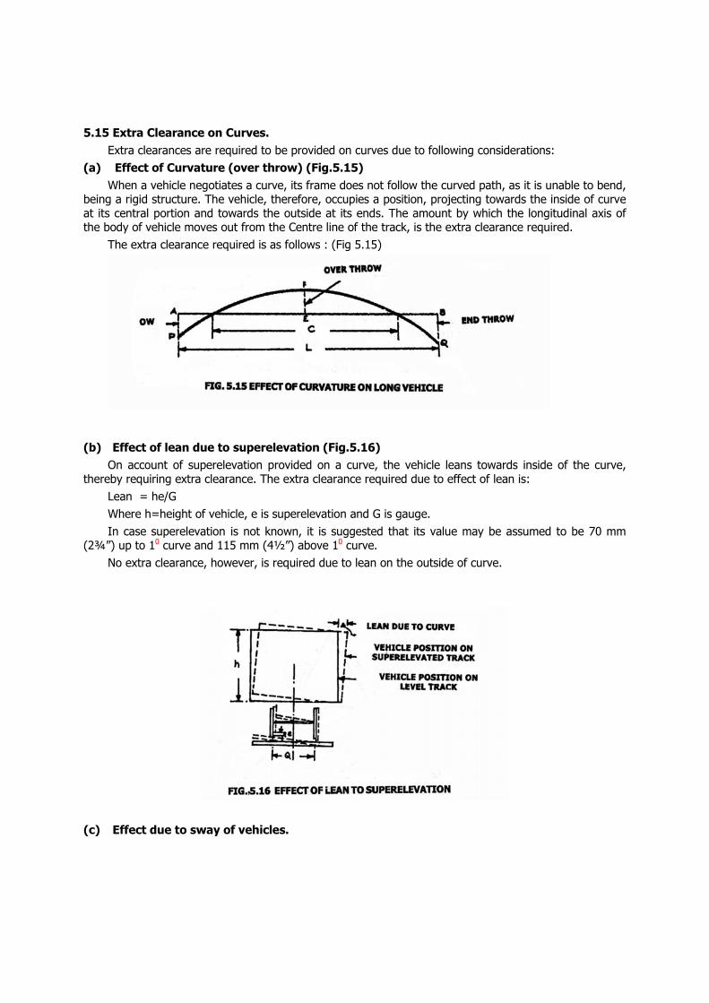
5.15 Extra Clearance on Curves. Extra clearances are required to be provided on curves due to following considerations:

(a) Effect of Curvature (over throw) (Fig.5.15) When a vehicle negotiates a curve, its frame does not follow the curved path, as it is unable to bend,

being a rigid structure. The vehicle, therefore, occupies a position, projecting towards the inside of curve at its central portion and towards the outside at its ends. The amount by which the longitudinal axis of the body of vehicle moves out from the Centre line of the track, is the extra clearance required.

The extra clearance required is as follows : (Fig 5.15)

(b) Effect of lean due to superelevation (Fig.5.16)

On account of superelevation provided on a curve, the vehicle leans towards inside of the curve, thereby requiring extra clearance. The extra clearance required due to effect of lean is:

Lean = he/G Where h=height of vehicle, e is superelevation and G is gauge. In case superelevation is not known, it is suggested that its value may be assumed to be 70 mm

(2¾”) up to 10 curve and 115 mm (4½”) above 10 curve. No extra clearance, however, is required due to lean on the outside of curve.

(c) Effect due to sway of vehicles.

On account of unbalanced centrifugal forces caused due to cant deficiency etc. the vehicles have a tendency of additional sway and extra clearance required on the inside of the curve due to the sway is taken to be 1/4th of the clearance necessary due to lean.

The empirical formula normally adopted in the field for extra clearance due to curvature effect is as given below:

B.G M.G. Overthrow (mm) : 27330/R 23516/R End throw (mm) : 29600/R 24063/R The above empirical formula is based on standard B.G. and M.G. bogie lengths and value of R is in

meters. 5.15.1 Extra clearance for platforms

In case of platforms, it has been observed that provision of extra clearance on curves as stipulated above may lead to excessive gap between the footboard and platform. It has therefore, been stipulated that this extra clearance will be reduced by 51 mm (2") on inside of the curve and 25 mm(1") on outside of the curve. 5.15.2 Widening of gauge or curves

A vehicle normally assumes the central position on a straight track and the flanges of the wheels are clear of rails. The position is however, different on a curved track. As soon as the vehicle enters a curve, the flange of the outside wheel of leading axle continues to travel in a straight line till it rubs against the rail. Due to coning of wheel, the outside wheel travels a longer distance compared to the inner wheel. This is however, not possible for the vehicle as a whole because due to rigidity of the wheel base, the trailing axle occupies a different position. In an effort to make up the difference of travel between outer wheel and inner wheel, the inside wheels slip backward and outer wheels skid forward. A close study of vehicles on curves indicate that wear of flanges cases the passage of a vehicle round curves as it has been effect of increasing the play. Widening of gauge on a curve has in effect the same effect and it tends to decrease wear and tear on both vehicles and track. 5.16 Compensation for Curvature on gradients

The ruling gradient is required to be compensated on curves to offset the extra resistance due to curvature. The curve resistance depends upon a number of variable factors, but for simplicity reasons it is taken as percentage per degree of curve. Compensation for curvature allowed on Indian Railways is as follows:

B.G…..0.04% per degree of curvature i.e. 0.04x1750/R = 7/R M.G….0.03%per degree of curvature i.e. 0.03x1750/R = 52.5/R N.G…..0.02% per degree of curvature i.e. 0.02x1750/R = 35/R Where, R is radius of the curve in meters. Problem. Find out the steepest gradient permissible on a 20 curve for BG line having ruling gradient

of 1 in 200. Solution. Ruling gradient = 1 in 200 = 0.5% = 0.04 x 20 = 0.08% Max. permissible gradient on curve = 0.5 – 0.08 = 0.42% 1 in 100/0.42 = in 238 The curve can have the steepest gradient of 1 in 238.

5.17 VERTICAL CURVES(Fig.5.17) Where two different gradients meet, an angle is formed at the junction forming summit or sag as explained in Fig 5.17.

The angle at the junction is smoothened by providing a curve in the vertical plane called “VERTICAL CURVE”. In the absence of a vertical curve, running on the tack is likely to be rough. Besides this, change in gradient may also cause bunching of vehicles in sags and variation in the tension of couplings in summits, resulting in train parting and bad riding. To avoid these ill effects, the change in gradients is smoothened by a vertical curve. A rising gradient is normally expressed as + ve and a falling gradient expressed as –ve.

A vertical curve is normally designed as a circular curve, the circular profile ensures a uniform rate of change of grade, which controls the rotational accelerations. 5.17.1 Existing rules regarding vertical curves on Indian Railways.

As per existing rules, vertical curves are provided only at junction of the grades where the algebraic difference between the grades equal to or more than 4mm per meter or 0.4 per cent.

The minimum radius of the vertical curve should be as follows:

Broad Gauge (BG) Meter Gauge (MG) Group Min Radius Group Min radius A 4000m all routes 2500m B 3000m C, D & E 2500m

5.17.2 Setting out a vertical curve A vertical curve can be set by various methods such as tangent correction methods and chord

deflection method etc. It is proposed to describe tangent correction method, which is considered simpler and more convenient for field staff. Tangent correction methods (Fig.5.18)

(i) Length of vertical curve is first calculated by using the formula given above. Chainages and

reduced levels of tangent points and apex are then worked out. (ii) Tangent corrections are then computed from formula: Y =cx2 And C = g1-g2/4.N Where Y = vertical ordinate

x = horizontal distance from springing point. G1 = gradient No. 1 (+ive for rising grades) G2 = gradient No.2 (-ive for falling grades) N = number of chords up to half length of the curve. (iii) Find out the elevations of the stations on the curve by adding algebraically the tangent

corrections on tangent OA. 5.18 Realignment of Curves

A railway curve is likely to get distored from its original alignment in course of time due to the following reasons:

(i) Unbalanced loading of inner rail and outer rail due to cant excess with slower speeds or cant deficiency with higher speeds than the equilibrium speeds for which cant has been provided.

(ii) Effect of large horizontal forces on the rails by passing trains. These forces tend to make a curve flatter at few locations and sharper at others and radius of the

curve thus varies from place to place. These give rough riding on the curve due to change in radial acceleration from place to place. Realignment of curve, therefore becomes necessary to restore smooth running on curves. 5.18.1 Criteria for realignment of curves

The Railway Board has prescribed the following criteria for realignment of curve: (i) Cumulative Frequency Diagram. For Group A and B routes the need for curve realignment

should be decided by drawing cumulative frequency diagram showing versine variation over the theoretical versine. For Group A and B routes, the versine variations as measured on 20 meter chord shall be limited to 4mm and 5mm respectively. Realignment should be taken up when the cumulative percentage of versines lying within these limits is less than 80. However, this diagram is obsolete.

(ii) Station to Station versine difference: The running over a curve depends not only on the difference between the actual versine but also on the station to station variation of the actual versine values. This is because it is the station to station variation of versisne which determines the rate of change of radial acceleration on which depends the riding comfort. The following stipulation have been made in this connection:

Broad Gauge: On curves where speeds are from 110 kmph to 140 kmph are permitted, the station to station variation of versines at station 10 m apart shall not exceed 10 mm (15mm for 110 kmph) and for speeds below 110 kmph and up to 50 kmph variations shall not exceed 20 mm and for speeds less than 50 kmph 40 mm or 20% of average versine of the circular portion ( in all above cases) whichever is more.

Metre Gauge: On curves where speeds in excess of 75 kmph are permitted, the station to station variation of versines at stations 10 meters apart shall not exceed 15 mm. for speeds of 75 kmph and less, such variations shall not exceed 20 mm or 20% of the average versine of the circular portion whichever is more.

(iii) The decision for complete realignment of a curve shall be taken on the basis of running on the curve, cumulative frequency diagram (obsolete) or on the basis of distribution of variation of versines between stations as indicated in paras above.

(iv) Unsatisfactory Running of Track : For other routes, curve realignment will be taken in hand when as a result of inspection by trolly or from the footplate of locomotive or by rear carriage or as a result of track tests carried out, the running on the curve is found to be unsatisfactory.

(v) Local adjustment : when there is abrupt variation of versines between adjacent stations local adjustments should be done to obtain versine variation between adjacent stations within reasonable limits. Such corrections should be carried in advance of complete curve realignment. 5.19 String Linging Method of Realignment of Curves. 5.19.1 General Principles

The realignment of existing curves with a theodolite is difficult and laborious work and the curves are therefore realigned by measuring versines with the help of string and correcting these versines; The method is known as ‘String Lining Method’ on the Indian Railways. The Method is based on the following basic principles.

(i) Sum of all versines taken on equal chords of any two curves between the same tangents are equal. If follows, from this, that the final value of the sum of the differences between the existing and proposed versine must be zero.

(ii) Throw at any station is equal to twice the 2nd summation of the differences of the proposed and existing versine up to the previous station. 5.19.2 Procedure for String Lining the Curve. The work of realignment of a curve by string lining method consists of the following three operations: (i) Survey of the existing curve by measurement of versines. (ii) Computation of slews including provisions of proper transition and superelevation for the revised

alignment. (iii) Slewing of the curve to the revised alignment.

5.20 Check rail on curve (Fig. 5.19) Check rails are basically provided on sharp curves on the inner rail to reduce the lateral wear, on the

outer rails. They also prevent the outer wheel flange from mounting on the outer rail and thus decrease the chances of derailment of the vehicles. Check rails wear out quite fast but as these are normally worn

rails unit for main line tracks, further wear of check rails is not considered objectionable.

As per present stipulations check rails are provided on the gauge face side of the inner rails on

curves sharper than 80 on B.G., 100 on M.G. and 140 on N.G. Minimum clearance prescribed for check rail is 44mm for B.G. and 41 mm for N.G.