Tracking GPS Signals

Fundamentals of Global Positioning System Receivers: A Software ApproachJames Bao-Yen Tsui

Copyright 2000 John Wiley & Sons, Inc.Print ISBN 0-471-38154-3 Electronic ISBN 0-471-20054-9

165

CHAPTER EIGHT

Tracking GPS Signals

8.1 INTRODUCTION

One might think that the basic method of tracking a signal is to build a narrow-band filter around an input signal and follow it. In other words, while the fre-quency of the input signal varies over time, the center frequency of the filtermust follow the signal. In the actual tracking process, the center frequency of thenarrow-band filter is fixed, but a locally generated signal follows the frequencyof the input signal. The phases of the input and locally generated signals arecompared through a phase comparator. The output from the phase comparatorpasses through a narrow-band filter. Since the tracking circuit has a very narrowbandwidth, the sensitivity is relatively high in comparison with the acquisitionmethod.

When there are phase shifts in the carrier due to the C/ A code, as in a GPSsignal, the code must be stripped off first as discussed in Section 7.5. The track-ing process will follow the signal and obtain the information of the navigationdata. If a GPS receiver is stationary, the expected frequency change due to satel-lite movement is very slow as discussed in Chapter 3. Under this condition, thefrequency change of the locally generated signal is also slow; therefore, theupdate rate of the tracking loop can be low. In order to strip off the C/ A codeanother loop is needed. Thus, to track a GPS signal two tracking loops arerequired. One loop is used to track the carrier frequency and is referred to asthe carrier loop. The other one is used to track the C/ A code and is referred toas the code loop.

In this chapter the basic loop concept will be discussed first. Two trackingmethods will be discussed. The first one is the conventional tracking loop. Theonly unique point of this method is that the tracking loop will be presentedin digital form and the tracking will be accomplished in software. The secondmethod is referred to as the block adjustment of synchronizing signal (BASS)method. The BASS method is also implemented in software and the perfor-

166 TRACKING GPS SIGNALS

mance might be slightly sensitive to noise. The details of the two methods willbe presented.

8.2 BASIC PHASE-LOCKED LOOPS(1–4)

In this section the basic concept of the phase-locked loop will be described,which includes the transfer function, the error transfer function, the noise band-width, and two types of input signals.

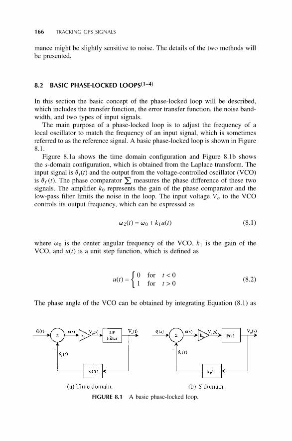
The main purpose of a phase-locked loop is to adjust the frequency of alocal oscillator to match the frequency of an input signal, which is sometimesreferred to as the reference signal. A basic phase-locked loop is shown in Figure8.1.

Figure 8.1a shows the time domain configuration and Figure 8.1b showsthe s-domain configuration, which is obtained from the Laplace transform. Theinput signal is v i(t) and the output from the voltage-controlled oscillator (VCO)is v f (t). The phase comparator ∑ measures the phase difference of these twosignals. The amplifier k0 represents the gain of the phase comparator and thelow-pass filter limits the noise in the loop. The input voltage Vo to the VCOcontrols its output frequency, which can be expressed as

q2(t) c q0 + k1u(t) (8.1)

where q0 is the center angular frequency of the VCO, k1 is the gain of theVCO, and u(t) is a unit step function, which is defined as

u(t) c { 0 for t < 01 for t > 0

(8.2)

The phase angle of the VCO can be obtained by integrating Equation (8.1) as

FIGURE 8.1 A basic phase-locked loop.

8.2 BASIC PHASE-LOCKED LOOPS 167

∫t

0q2(t)dt c q0t + v f (t) c q0t + ∫

t

0k1u(t)dt

where v f (t) c ∫t

0k1u(t)dt (8.3)

The Laplace transform of v f (t) is

v f (s) c k1

s(8.4)

From Figure 8.1b the following equations can be written.

Vc(s) c k0e(s) c k0[v i(s) − v f (s)] (8.5)

Vo(s) c Vc(s)F (s) (8.6)

v f (s) c Vo(s)k1

s(8.7)

From these three equations one can obtain

e(s) c v i(s) − v f (s) c Vc(s)k0

c Vo(s)k0F (s)

c sv f (s)k0k1F (s)

or

v i(s) c v f (s) �1 +s

k0k1F (s) � (8.8)

where e(s) is the error function. The transfer function H(s) of the loop is definedas

H(s) ≡v f (s)v i(s)

c k0k1F (s)s + k0k1F (s)

(8.9)

The error transfer function is defined as

He(s) c e(s)v i(s)

c v i(s) − v f (s)v i(s)

c 1 − H(s) c ss + k0k1F (s)

(8.10)

The equivalent noise bandwidth is defined as(1)


Bn c ∫∞

0|H( jq) | 2d f (8.11)

where q is the angular frequency and it relates to the frequency f by q c 2pf .In order to study the properties of the phase-locked loops, two types of input

signals are usually studied. The first type is a unit step function as

v i(t) c u(t) or v i(s) c 1s

(8.12)

The second type is a frequency-modulated signal

v i(t) c Dqt or v i(s) c Dq

s2(8.13)

These two types of signals will be discussed in the next two sections.

8.3 FIRST-ORDER PHASE-LOCKED LOOP(1–4)

In this section, the first-order phase-locked loop will be discussed. A first-orderphase-locked loop implies the denominator of the transfer function H(s) is afirst-order function of s. The order of the phase-locked loop depends on theorder of the filter in the loop. For this kind of phase-locked loop, the filterfunction is

F(s) c 1 (8.14)

This is the simplest phase-locked loop. For a unit step function input, the cor-responding transfer function from Equation (8.9) becomes

H(s) c k0k1

s + k0k1(8.15)

The denominator of H(s) is a first order of s.The noise bandwidth can be found as

Bn c ∫∞

0

(k0k1)2d fq2 + (k0k1)2

c (k0k1)2

2p ∫∞

0

dq

q2 + (k0k1)2

c (k0k1)2

2pk0k1tan−1 � q

k0k1�

∞

0

c k0k1

4(8.16)

8.4 SECOND-ORDER PHASE-LOCKED LOOP 169

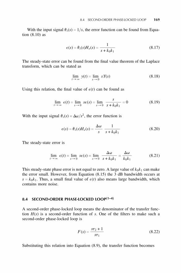
With the input signal v i(s) c 1/ s, the error function can be found from Equa-tion (8.10) as

e(s) c v i(s)He(s) c 1s + k0k1

(8.17)

The steady-state error can be found from the final value theorem of the Laplacetransform, which can be stated as

limt r ∞

y(t) c lims r 0

sY(s) (8.18)

Using this relation, the final value of e(t) can be found as

limt r ∞

e(t) c lims r 0

se(s) c lims r 0

ss + k0k1

c 0 (8.19)

With the input signal v i(s) c Dq/ s2, the error function is

e(s) c v i(s)He(s) c Dq

s1

s + k0k1(8.20)

The steady-state error is

limt r ∞

e(t) c lims r 0

se(s) c lims r 0

Dq

s + k0k1c Dq

k0k1(8.21)

This steady-state phase error is not equal to zero. A large value of k0k1 can makethe error small. However, from Equation (8.15) the 3 dB bandwidth occurs ats c k0k1. Thus, a small final value of e(t) also means large bandwidth, whichcontains more noise.

8.4 SECOND-ORDER PHASE-LOCKED LOOP(1–4)

A second-order phase-locked loop means the denominator of the transfer func-tion H(s) is a second-order function of s. One of the filters to make such asecond-order phase-locked loop is

F (s) c st2 + 1st1

(8.22)

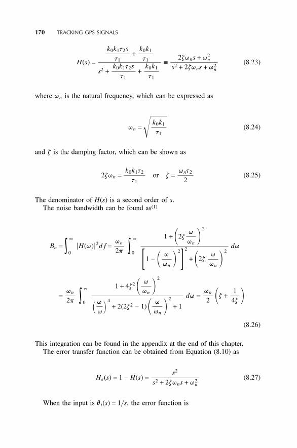
Substituting this relation into Equation (8.9), the transfer function becomes


H(s) ck0k1t2s

t1+

k0k1

t1

s2 +k0k1t2s

t1+

k0k1

t1

≡2zqns + q2

n

s2 + 2zqns + q2n

(8.23)

where qn is the natural frequency, which can be expressed as

qn ci

k0k1

t1(8.24)

and z is the damping factor, which can be shown as

2zqn c k0k1t2

t1or z c qnt2

2(8.25)

The denominator of H(s) is a second order of s.The noise bandwidth can be found as(1)

Bn c ∫∞

0|H(q) | 2d f c qn

2p ∫∞

0

1 + �2zq

qn�

2

[1 − � q

qn�

2] 2

+ �2zq

qn�

2dq

c qn

2p ∫∞

0

1 + 4z2 � q

qn�

2

�q

q �4

+ 2(2z2 − 1) � q

qn�

2

+ 1

dq c qn

2 �z +14z �

(8.26)

This integration can be found in the appendix at the end of this chapter.The error transfer function can be obtained from Equation (8.10) as

He(s) c 1 − H(s) c s2

s2 + 2zqns + q2n

(8.27)

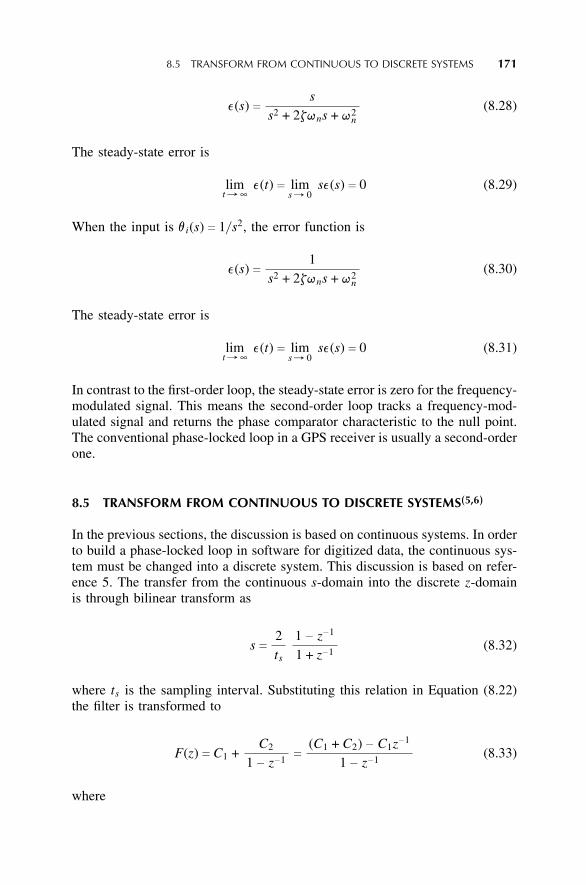
When the input is v i(s) c 1/ s, the error function is

8.5 TRANSFORM FROM CONTINUOUS TO DISCRETE SYSTEMS 171

e(s) c ss2 + 2zqns + q2

n(8.28)


limt r ∞

e(t) c lims r 0

se(s) c 0 (8.29)

When the input is v i(s) c 1/ s2, the error function is

e(s) c 1s2 + 2zqns + q2

n(8.30)


limt r ∞

e(t) c lims r 0

se(s) c 0 (8.31)

In contrast to the first-order loop, the steady-state error is zero for the frequency-modulated signal. This means the second-order loop tracks a frequency-mod-ulated signal and returns the phase comparator characteristic to the null point.The conventional phase-locked loop in a GPS receiver is usually a second-orderone.

8.5 TRANSFORM FROM CONTINUOUS TO DISCRETE SYSTEMS(5,6)

In the previous sections, the discussion is based on continuous systems. In orderto build a phase-locked loop in software for digitized data, the continuous sys-tem must be changed into a discrete system. This discussion is based on refer-ence 5. The transfer from the continuous s-domain into the discrete z-domainis through bilinear transform as

s c 2ts

1 − z−1

1 + z−1(8.32)

where ts is the sampling interval. Substituting this relation in Equation (8.22)the filter is transformed to

F(z) c C1 +C2

1 − z−1c (C1 + C2) − C1z−1

1 − z−1(8.33)

where


FIGURE 8.2 Loop filter.

C1 c 2t2 − ts

2t1

C2 c ts

t1(8.34)

This filter is shown in Figure 8.2.The VCO in the phase-locked loop is replaced by a direct digital frequency

synthesizer and its transfer function N(z) can be used to replace the result inEquation (8.7) with

N(z) c v f (z)Vo(z)

≡k1z−1

1 − z−1(8.35)

Using the same approach as Equation (8.8), the transfer function H(z) can bewritten as

H(z) c v f (z)v i(z)

c k0F(z)N(z)1 + k0F(z)N(z)

(8.36)

Substituting the results of Equations (8.33) and (8.35) into the above equation,the result is

H(z) c k0k1(C1 + C2)z−1 − k0k1C1z−2

1 + [k0k1(C1 + C2) − 2]z−1 + (1 − k0k1C1)z−2(8.37)

By applying bilinear transform in Equation (8.32) to Equation (8.23), the resultcan be written as,

8.6 CARRIER AND CODE TRACKING 173

H(z) c [4zqn + (qnts)2] + 2(qnts)2z−1 + [(qnts)2 − rzqnts]z−2

[4 + 4zqnts + (qnts)2] + [2(qnts)2 − 8]z−1 + [4 − 4zqnts + (qnts)2]z−2

(8.38)

By equating the denominator polynomials in the above two equations, C1 andC2 can be found as

C1 c 1k0k1

8zqnts

4 + 4zqnts + (qnts)2

C2 c 1k0k1

4(qnts)2

4 + 4zqnts + (qnts)2(8.39)

The applications of these equations will be discussed in the next two sections.In reference 6 a third-order phase-locked loop is also implemented. The filter

is implemented in digital format and the result can be used for phase-lockedloop designs, but it is not included in this book.

8.6 CARRIER AND CODE TRACKING(4)

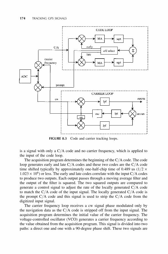
Before discussing the usage of the above equations, let us concentrate on thetracking of GPS signals. The input to a conventional phase-locked loop is usu-ally a continuous wave (cw) or frequency-modulated signal and the frequencyof the VCO is controlled to follow the frequency of the input signal. In a GPSreceiver the input is the GPS signal and a phase-locked loop must follow (ortrack) this signal. However, the GPS signal is a bi-phase coded signal. The car-rier and code frequencies change due to the Doppler effect, which is caused bythe motion of the GPS satellite as well as from the motion of the GPS receiveras discussed in Chapter 3. In order to track the GPS signal, the C/ A code infor-mation must be removed. As a result, it requires two phase-locked loops to tracka GPS signal. One loop is to track the C/ A code and the other one is to trackthe carrier frequency. These two loops must be coupled together as shown inFigure 8.3.

In Figure 8.3, the C/ A code loop generates three outputs: an early code, alate code, and a prompt code. The prompt code is applied to the digitized inputsignal and strips the C/ A code from the input signal. Stripping the C/ A codemeans to multiply the C/ A code to the input signal with the proper phase asshown in Figure 7.1. The output will be a cw signal with phase transition causedonly by the navigation data. This signal is applied to the input of the carrierloop. The output from the carrier loop is a cw with the carrier frequency ofthe input signal. This signal is used to strip the carrier from the digitized inputsignal, which means using this signal to multiply the input signal. The output


FIGURE 8.3 Code and carrier tracking loops.

is a signal with only a C/ A code and no carrier frequency, which is applied tothe input of the code loop.

The acquisition program determines the beginning of the C/ A code. The codeloop generates early and late C/ A codes and these two codes are the C/ A codetime shifted typically by approximately one-half-chip time of 0.489 us (1/ 2 ×1.023 × 106) or less. The early and late codes correlate with the input C/ A codesto produce two outputs. Each output passes through a moving average filter andthe output of the filter is squared. The two squared outputs are compared togenerate a control signal to adjust the rate of the locally generated C/ A codeto match the C/ A code of the input signal. The locally generated C/ A code isthe prompt C/ A code and this signal is used to strip the C/ A code from thedigitized input signal.

The carrier frequency loop receives a cw signal phase modulated only bythe navigation data as the C/ A code is stripped off from the input signal. Theacquisition program determines the initial value of the carrier frequency. Thevoltage-controlled oscillator (VCO) generates a carrier frequency according tothe value obtained from the acquisition program. This signal is divided into twopaths: a direct one and one with a 90-degree phase shift. These two signals are

8.7 USING THE PHASE-LOCKED LOOP TO TRACK GPS SIGNALS 175

correlated with the input signal. The outputs of the correlators are filtered andtheir phases are compared against each other through an arctangent comparator.The arctangent operation is insensitive to the phase transition caused by thenavigation data and it can be considered as one type of a Costas loop. A Costasloop is a phase-locked loop, which is insensitive to phase transition. The outputof the comparator is filtered again and generates a control signal. This controlsignal is used to tune the oscillator to generate a carrier frequency to followthe input cw signal. This carrier frequency is also used to strip the carrier fromthe input signal.

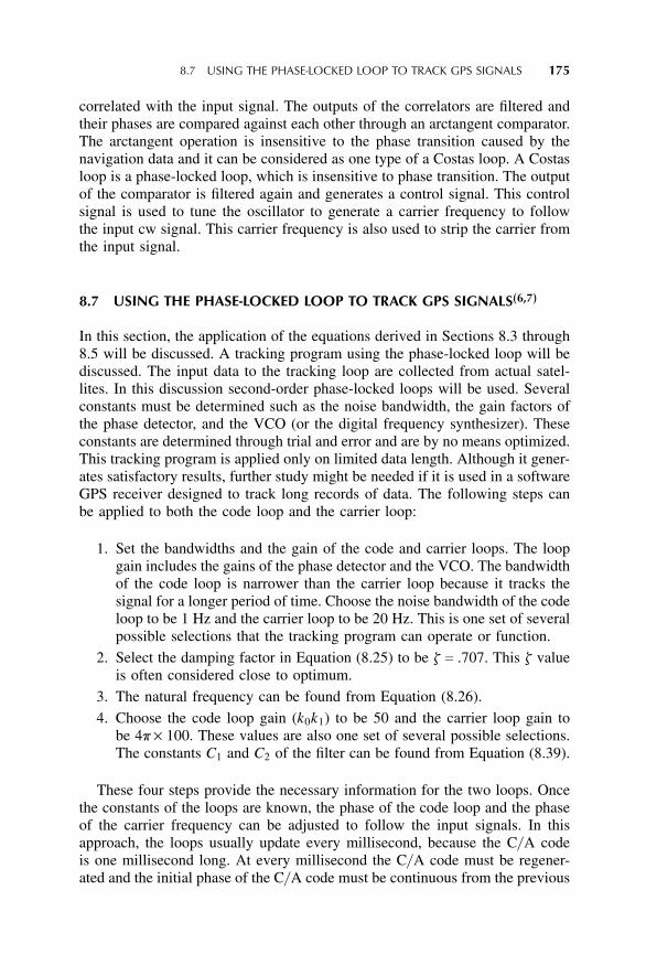
8.7 USING THE PHASE-LOCKED LOOP TO TRACK GPS SIGNALS(6,7)

In this section, the application of the equations derived in Sections 8.3 through8.5 will be discussed. A tracking program using the phase-locked loop will bediscussed. The input data to the tracking loop are collected from actual satel-lites. In this discussion second-order phase-locked loops will be used. Severalconstants must be determined such as the noise bandwidth, the gain factors ofthe phase detector, and the VCO (or the digital frequency synthesizer). Theseconstants are determined through trial and error and are by no means optimized.This tracking program is applied only on limited data length. Although it gener-ates satisfactory results, further study might be needed if it is used in a softwareGPS receiver designed to track long records of data. The following steps canbe applied to both the code loop and the carrier loop:

1. Set the bandwidths and the gain of the code and carrier loops. The loopgain includes the gains of the phase detector and the VCO. The bandwidthof the code loop is narrower than the carrier loop because it tracks thesignal for a longer period of time. Choose the noise bandwidth of the codeloop to be 1 Hz and the carrier loop to be 20 Hz. This is one set of severalpossible selections that the tracking program can operate or function.

2. Select the damping factor in Equation (8.25) to be z c .707. This z valueis often considered close to optimum.

3. The natural frequency can be found from Equation (8.26).

4. Choose the code loop gain (k0k1) to be 50 and the carrier loop gain tobe 4p × 100. These values are also one set of several possible selections.The constants C1 and C2 of the filter can be found from Equation (8.39).

These four steps provide the necessary information for the two loops. Oncethe constants of the loops are known, the phase of the code loop and the phaseof the carrier frequency can be adjusted to follow the input signals. In thisapproach, the loops usually update every millisecond, because the C/ A codeis one millisecond long. At every millisecond the C/ A code must be regener-ated and the initial phase of the C/ A code must be continuous from the previous


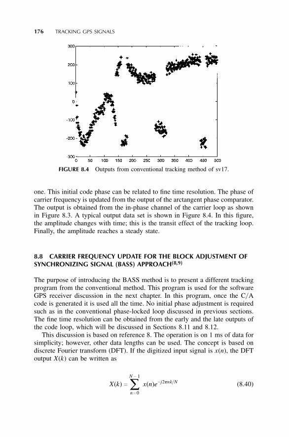
FIGURE 8.4 Outputs from conventional tracking method of sv17.

one. This initial code phase can be related to fine time resolution. The phase ofcarrier frequency is updated from the output of the arctangent phase comparator.The output is obtained from the in-phase channel of the carrier loop as shownin Figure 8.3. A typical output data set is shown in Figure 8.4. In this figure,the amplitude changes with time; this is the transit effect of the tracking loop.Finally, the amplitude reaches a steady state.

8.8 CARRIER FREQUENCY UPDATE FOR THE BLOCK ADJUSTMENT OF

SYNCHRONIZING SIGNAL (BASS) APPROACH(8,9)

The purpose of introducing the BASS method is to present a different trackingprogram from the conventional method. This program is used for the softwareGPS receiver discussion in the next chapter. In this program, once the C/ Acode is generated it is used all the time. No initial phase adjustment is requiredsuch as in the conventional phase-locked loop discussed in previous sections.The fine time resolution can be obtained from the early and the late outputs ofthe code loop, which will be discussed in Sections 8.11 and 8.12.

This discussion is based on reference 8. The operation is on 1 ms of data forsimplicity; however, other data lengths can be used. The concept is based ondiscrete Fourier transform (DFT). If the digitized input signal is x(n), the DFToutput X(k) can be written as

X(k) c N − 1

∑n c 0

x(n)e− j2pnk/ N (8.40)

8.8 CARRIER FREQUENCY UPDATE FOR THE BLOCK ADJUSTMENT 177

where k represents a certain frequency component and N is the total number ofdata points. If x(n) is obtained from digitizing a sinusoidal wave, the highestamplitude |X(ki) | represents the frequency of the input signal. The real (Re)and imaginary (Im) parts of X(k1) can be used to obtain phase angle v as

v c tan−1 � Im[X(ki)]Re[X(ki)] � (8.41)

where v presents the initial phase of the sine wave with respect to the Kernelfunction. If k is an integer, the initial phase of the Kernel function is zero. Ingeneral, if the frequency of the input signal is an unknown quantity, all thecomponents of k (k c 0 ∼ N − 1) must be calculated. However, only half ofthe k values (k c 0 ∼ N/ 2 − 1) provide useful information as discussed inSection 6.13. The highest component X(ki) can be found by comparing all theX(k) values. For this operation, the fast Fourier transform (FFT) is often usedto save calculation time.

If the frequency of the input signal can be found within a frequency resolu-tion cell, which is equal to 1/ Nts (where ts is the sampling time), the desiredX(k) can be found from one component of the DFT. It should be noted that tocalculate one component of X(k), the k value need not be an integer as in thecase of FFT. Since the input frequency is estimated from the acquisition method,the X(k) can be found from one k value of Equation (8.40). The purpose of thisoperation is to find the fine frequency of the input signal.

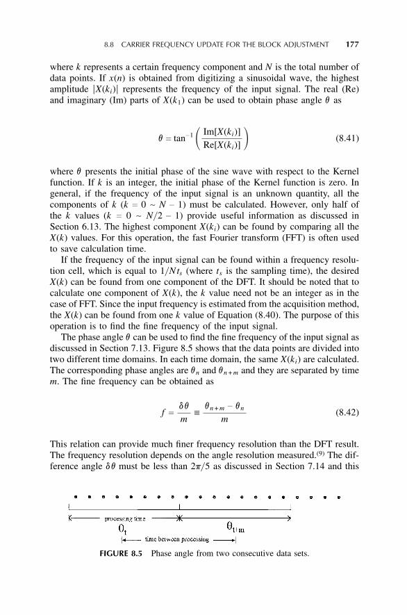
The phase angle v can be used to find the fine frequency of the input signal asdiscussed in Section 7.13. Figure 8.5 shows that the data points are divided intotwo different time domains. In each time domain, the same X(ki) are calculated.The corresponding phase angles are vn and vn + m and they are separated by timem. The fine frequency can be obtained as

f c dv

m≡

vn + m − vn

m(8.42)

This relation can provide much finer frequency resolution than the DFT result.The frequency resolution depends on the angle resolution measured.(9) The dif-ference angle dv must be less than 2p/ 5 as discussed in Section 7.14 and this

FIGURE 8.5 Phase angle from two consecutive data sets.


requirement limits the time between the two consecutive DFT calculations.Since the frequency k is very close to the input frequency, which changes slowlywith time, the unambiguous frequency range is not a problem. This approachis used to find the correct frequency and update it accordingly.

8.9 DISCONTINUITY IN KERNEL FUNCTION

In conventional DFT operation the k value in Equation 8.40 is an integer. How-ever, in applying Equation (8.40) to the tracking program the k value is usually anoninteger, because in using an integer value of k, the frequency generated fromthe kernel function e− j2pnk/ N can be too far from the input frequency. If the k valueis far from the input signal, the amplitude of X(k) obtained from Equation (8.40)will be small, which implies that the sensitivity of the processing is low. In orderto avoid this problem, the k value should be kept as close to the input frequencyas possible. A k value close to the input frequency can also reduce the frequencyambiguity. Under this condition, the k value is usually no longer an integer.

When the k value is an integer, the initial phase of the Kernel functione− j2pnk/ N is zero and the values obtained from two consecutive sets are con-tinuous. The beginning point of the first set is n c 0 and the beginning point ofthe second set is n c N. It is easily shown that

e− j2pnk/ N | n c 0 c e− j2pnk/ N | n cN if k c integer (8.43)

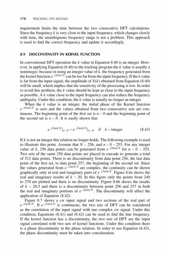
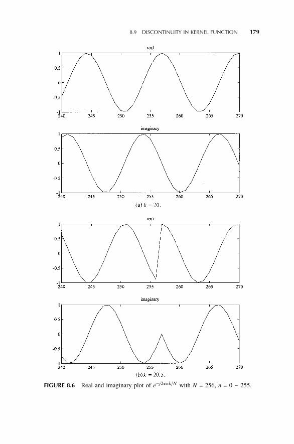
If k is not an integer this relation no longer holds. The following example is usedto illustrate this point. Assume that N c 256, and n c 0 ∼ 255. For any integervalue of k, 256 data points can be generated from e− j2pnk/ N for n c 0 ∼ 255.Two sets of the same 256 data points are placed in cascade to generate a totalof 512 data points. There is no discontinuity from data point 256, the last datapoint of the first set, to data point 257, the beginning of the second set. Sincethe values generated from e− j2pnk/ N are complex, the continuity can be showngraphically only in real and imaginary parts of e− j2pnk/ N . Figure 8.6a shows thereal and imaginary results of k c 20. In this figure only the points from 240to 270 are plotted and there is no discontinuity. Figure 8.6b shows the resultsof k c 20.5 and there is a discontinuity between point 256 and 257 in boththe real and imaginary portions of e− j2pnk/ N . The discontinuity will affect theapplication of Equation (8.42).

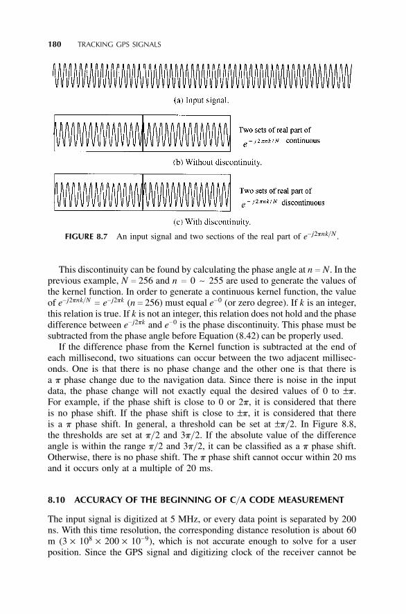
Figure 8.7 shows a cw input signal and two sections of the real part ofe− j2pnk/ N . If e− j2pnk/ N is continuous, the two sets of DFT can be consideredas the correlation of the input signal with one complex cw signal. Under thiscondition, Equations (8.41) and (8.42) can be used to find the fine frequency.If the kernel function has a discontinuity, the two sets of DFT are the inputsignal correlated with two sets of kernel functions. Under this condition thereis a phase discontinuity in the phase relation. In order to use Equation (8.42),the phase discontinuity must be taken into consideration.

8.9 DISCONTINUITY IN KERNEL FUNCTION 179

FIGURE 8.6 Real and imaginary plot of e− j2pnk/ N with N c 256, n c 0 ∼ 255.


FIGURE 8.7 An input signal and two sections of the real part of e− j2pnk/ N .

This discontinuity can be found by calculating the phase angle at n c N. In theprevious example, N c 256 and n c 0 ∼ 255 are used to generate the values ofthe kernel function. In order to generate a continuous kernel function, the valueof e− j2pnk/ N c e− j2pk (n c 256) must equal e−0 (or zero degree). If k is an integer,this relation is true. If k is not an integer, this relation does not hold and the phasedifference between e− j2pk and e−0 is the phase discontinuity. This phase must besubtracted from the phase angle before Equation (8.42) can be properly used.

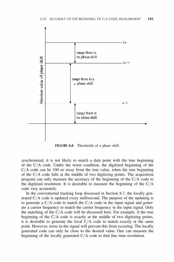
If the difference phase from the Kernel function is subtracted at the end ofeach millisecond, two situations can occur between the two adjacent millisec-onds. One is that there is no phase change and the other one is that there isa p phase change due to the navigation data. Since there is noise in the inputdata, the phase change will not exactly equal the desired values of 0 to ±p.For example, if the phase shift is close to 0 or 2p, it is considered that thereis no phase shift. If the phase shift is close to ±p, it is considered that thereis a p phase shift. In general, a threshold can be set at ±p/ 2. In Figure 8.8,the thresholds are set at p/ 2 and 3p/ 2. If the absolute value of the differenceangle is within the range p/ 2 and 3p/ 2, it can be classified as a p phase shift.Otherwise, there is no phase shift. The p phase shift cannot occur within 20 msand it occurs only at a multiple of 20 ms.

8.10 ACCURACY OF THE BEGINNING OF C/ A CODE MEASUREMENT

The input signal is digitized at 5 MHz, or every data point is separated by 200ns. With this time resolution, the corresponding distance resolution is about 60m (3 × 108 × 200 × 10−9), which is not accurate enough to solve for a userposition. Since the GPS signal and digitizing clock of the receiver cannot be

8.10 ACCURACY OF THE BEGINNING OF C/ A CODE MEASUREMENT 181

FIGURE 8.8 Thresholds of a phase shift.

synchronized, it is not likely to match a data point with the true beginningof the C/ A code. Under the worst condition, the digitized beginning of theC/ A code can be 100 ns away from the true value, when the true beginningof the C/ A code falls at the middle of two digitizing points. The acquisitionprogram can only measure the accuracy of the beginning of the C/ A code tothe digitized resolution. It is desirable to measure the beginning of the C/ Acode very accurately.

In the conventional tracking loop discussed in Section 8.7, the locally gen-erated C/ A code is updated every millisecond. The purpose of the updating isto generate a C/ A code to match the C/ A code in the input signal and gener-ate a carrier frequency to match the carrier frequency in the input signal. Onlythe matching of the C/ A code will be discussed here. For example, if the truebeginning of the C/ A code is exactly at the middle of two digitizing points,it is desirable to generate the local C/ A code to match exactly at the samepoint. However, noise in the signal will prevent this from occuring. The locallygenerated code can only be close to the desired value. One can measure thebeginning of the locally generated C/ A code to find fine time resolution.


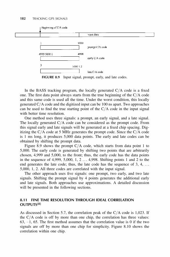
FIGURE 8.9 Input signal, prompt, early, and late codes.

In the BASS tracking program, the locally generated C/ A code is a fixedone. The first data point always starts from the true beginning of the C/ A codeand this same code is used all the time. Under the worst condition, this locallygenerated C/ A code and the digitized input can be 100 ns apart. Two approachescan be used to find the true starting point of the C/ A code in the input signalwith better time resolution.

One method uses three signals: a prompt, an early signal, and a late signal.The locally generated C/ A code can be considered as the prompt code. Fromthis signal early and late signals will be generated at a fixed chip spacing. Dig-itizing the C/ A code at 5 MHz generates the prompt code. Since the C/ A codeis 1 ms long, it produces 5,000 data points. The early and late codes can beobtained by shifting the prompt data.

Figure 8.9 shows the prompt C/ A code, which starts from data point 1 to5,000. The early code is generated by shifting two points that are arbitrarilychosen, 4,999 and 5,000, to the front; thus, the early code has the data pointsin the sequence of 4,999, 5,000, 1, 2 . . . 4,998. Shifting points 1 and 2 to theend generates the late code; thus, the late code has the sequence of 3, 4, . . .5,000, 1, 2. All three codes are correlated with the input signal.

The other approach uses five signals: one prompt, two early, and two latesignals. Shifting the prompt signal by 4 points generates the additional earlyand late signals. Both approaches use approximations. A detailed discussionwill be presented in the following sections.

8.11 FINE TIME RESOLUTION THROUGH IDEAL CORRELATION

OUTPUTS(8)

As discussed in Section 5.7, the correlation peak of the C/ A code is 1,023. Ifthe C/ A code is off by more than one chip, the correlation has three values:63, −1, 65. The first method assumes that the correlation value is 0 if the twosignals are off by more than one chip for simplicity. Figure 8.10 shows thecorrelation within one chip.

8.11 FINE TIME RESOLUTION THROUGH IDEAL CORRELATION OUTPUTS 183

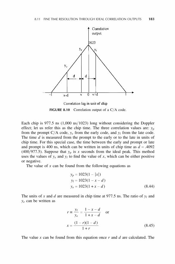
FIGURE 8.10 Correlation output of a C/ A code.

Each chip is 977.5 ns (1,000 us/ 1023) long without considering the Dopplereffect; let us refer this as the chip time. The three correlation values are: yp

from the prompt C/ A code, ye from the early code, and yl from the late code.The time d is measured from the prompt to the early or to the late in units ofchip time. For this special case, the time between the early and prompt or lateand prompt is 400 ns, which can be written in units of chip time as d c .4092(400/ 977.5). Suppose that yp is x seconds from the ideal peak. This methoduses the values of ye and yl to find the value of x, which can be either positiveor negative.

The value of x can be found from the following equations as

yp c 1023(1 − |x | )yl c 1023(1 − x − d )

ye c 1023(1 + x − d ) (8.44)

The units of x and d are measured in chip time at 977.5 ns. The ratio of yl andye can be written as

r ≡yl

yec 1 − x − d

1 + x − dor

x c (1 − r)(1 − d )1 + r

(8.45)

The value x can be found from this equation once r and d are calculated. The


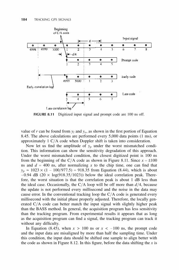
FIGURE 8.11 Digitized input signal and prompt code are 100 ns off.

value of r can be found from yl and ye, as shown in the first portion of Equation8.45. The above calculations are performed every 5,000 data points (1 ms), orapproximately 1 C/ A code when Doppler shift is taken into consideration.

Now let us find the amplitude of yp under the worst mismatched condi-tion. This information can show the sensitivity degradation of this approach.Under the worst mismatched condition, the closest digitized point is 100 nsfrom the beginning of the C/ A code as shown in Figure 8.11. Since x c ±100ns and d c 400 ns, after normalizing x to the chip time, one can find thatyp ≈ 1023 × (1 − 100/ 977.5) c 918.35 from Equation (8.44), which is about−0.94 dB (20 × log(918.35/ 1023)) below the ideal correlation peak. There-fore, the worst situation is that the correlation peak is about 1 dB less thanthe ideal case. Occasionally, the C/ A loop will be off more than d/ 4, becausethe update is not performed every millisecond and the noise in the data maycause error. In the conventional tracking loop the C/ A code is generated everymillisecond with the initial phase properly adjusted. Therefore, the locally gen-erated C/ A code can better match the input signal with slightly higher peakthan the BASS method. In general, the acquisition program has less sensitivitythan the tracking program. From experimental results it appears that as longas the acquisition program can find a signal, the tracking program can track itwithout any difficulty.

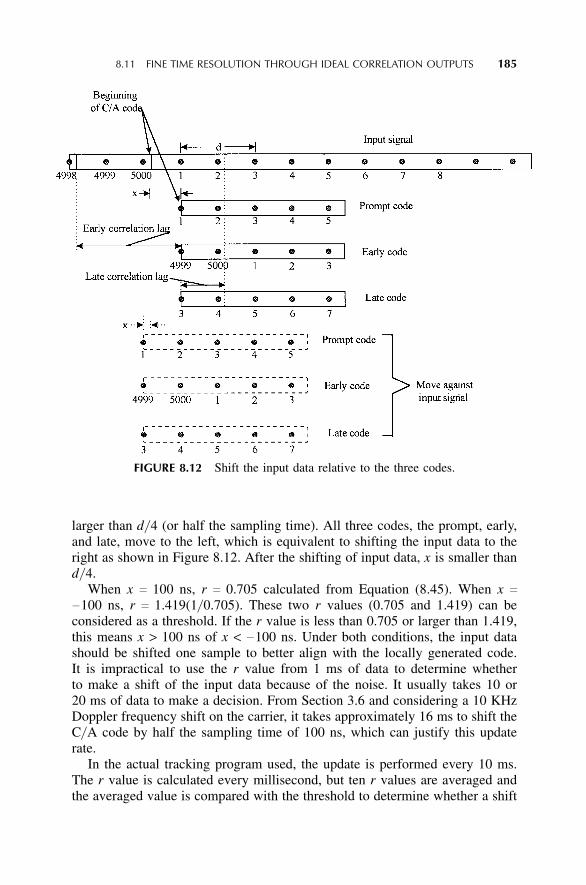
In Equation (8.45), when x > 100 ns or x < −100 ns, the prompt codeand the input data are misaligned by more than half the sampling time. Underthis condition, the input data should be shifted one sample to align better withthe code as shown in Figure 8.12. In this figure, before the data shifting the x is

8.11 FINE TIME RESOLUTION THROUGH IDEAL CORRELATION OUTPUTS 185

FIGURE 8.12 Shift the input data relative to the three codes.

larger than d/ 4 (or half the sampling time). All three codes, the prompt, early,and late, move to the left, which is equivalent to shifting the input data to theright as shown in Figure 8.12. After the shifting of input data, x is smaller thand/ 4.

When x c 100 ns, r c 0.705 calculated from Equation (8.45). When x c−100 ns, r c 1.419(1/ 0.705). These two r values (0.705 and 1.419) can beconsidered as a threshold. If the r value is less than 0.705 or larger than 1.419,this means x > 100 ns of x < −100 ns. Under both conditions, the input datashould be shifted one sample to better align with the locally generated code.It is impractical to use the r value from 1 ms of data to determine whetherto make a shift of the input data because of the noise. It usually takes 10 or20 ms of data to make a decision. From Section 3.6 and considering a 10 KHzDoppler frequency shift on the carrier, it takes approximately 16 ms to shift theC/ A code by half the sampling time of 100 ns, which can justify this updaterate.

In the actual tracking program used, the update is performed every 10 ms.The r value is calculated every millisecond, but ten r values are averaged andthe averaged value is compared with the threshold to determine whether a shift


FIGURE 8.13 Correlation Output with Limited Bandwidth.

in input data is needed. The x value calculated from the averaged r valuethrough Equation (8.45) is considered as the fine time resolution.

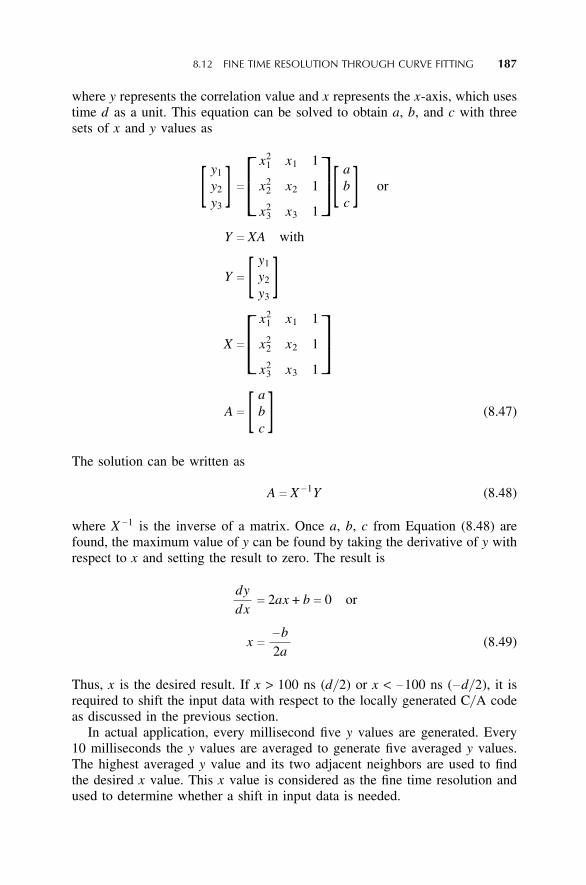
8.12 FINE TIME RESOLUTION THROUGH CURVE FITTING

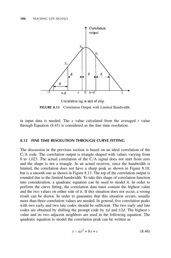
The discussion in the previous section is based on an ideal correlation of theC/ A code. The correlation output is triangle shaped with values varying from0 to 1,023. The actual correlation of the C/ A signal does not start from zeroand the shape is not a triangle. In an actual receiver, since the bandwidth islimited, the correlation does not have a sharp peak as shown in Figure 8.10,but is a smooth one as shown in Figure 8.13. The top of the correlation output isrounded due to the limited bandwidth. To take this shape of correlation functioninto consideration, a quadratic equation can be used to model it. In order toperform the curve fitting, the correlation data must contain the highest valueand the two values on either side of it. If this situation does not occur, a wrongresult can be drawn. In order to guarantee that this situation occurs, usuallymore than three correlation values are needed. In general, five correlation peakswith two early and two late codes should be sufficient. The two early and latecodes are obtained by shifting the prompt code by ±d and ±2d. The highest yvalue and its two adjacent neighbors are used in the following equation. Thequadratic equation to model the correlation peak can be written as

y c ax2 + bx + c (8.46)

8.12 FINE TIME RESOLUTION THROUGH CURVE FITTING 187

where y represents the correlation value and x represents the x-axis, which usestime d as a unit. This equation can be solved to obtain a, b, and c with threesets of x and y values as

[ y1

y2

y3] c

x21 x1 1

x22 x2 1

x23 x3 1

[ abc ] or

Y c XA with

Y c [ y1

y2

y3]

X c

x21 x1 1

x22 x2 1

x23 x3 1

A c [ abc ] (8.47)

The solution can be written as

A c X −1Y (8.48)

where X −1 is the inverse of a matrix. Once a, b, c from Equation (8.48) arefound, the maximum value of y can be found by taking the derivative of y withrespect to x and setting the result to zero. The result is

dydx

c 2ax + b c 0 or

x c −b2a

(8.49)

Thus, x is the desired result. If x > 100 ns (d/ 2) or x < −100 ns (−d/ 2), it isrequired to shift the input data with respect to the locally generated C/ A codeas discussed in the previous section.

In actual application, every millisecond five y values are generated. Every10 milliseconds the y values are averaged to generate five averaged y values.The highest averaged y value and its two adjacent neighbors are used to findthe desired x value. This x value is considered as the fine time resolution andused to determine whether a shift in input data is needed.


This method and the method discussed in Section 8.11 are both used inthe BASS tracking program. The differences between these two programs areinsignificant. The results from the method discussed in Section 8.11 are usedin Chapter 9.

8.13 OUTPUTS FROM THE BASS TRACKING PROGRAM

Besides the phase angles measured through the BASS program, two additionaloutputs are important for calculating user position. One is the beginning of theC/ A code and the other is the fine time resolution. Since the update is performedevery 10 ms, the shift of the beginning of the C/ A code is checked at this rate.If the misalignment between the locally generated C/ A code and the input datais more than 100 ns, the input data must be shifted either to the right or to theleft one data point to better match the local generated code. The actual startingpoints (reference to the input data points) of the C/ A code for every 10 msmust be kept. They will be used in the next chapter to find the beginning ofthe subframes.

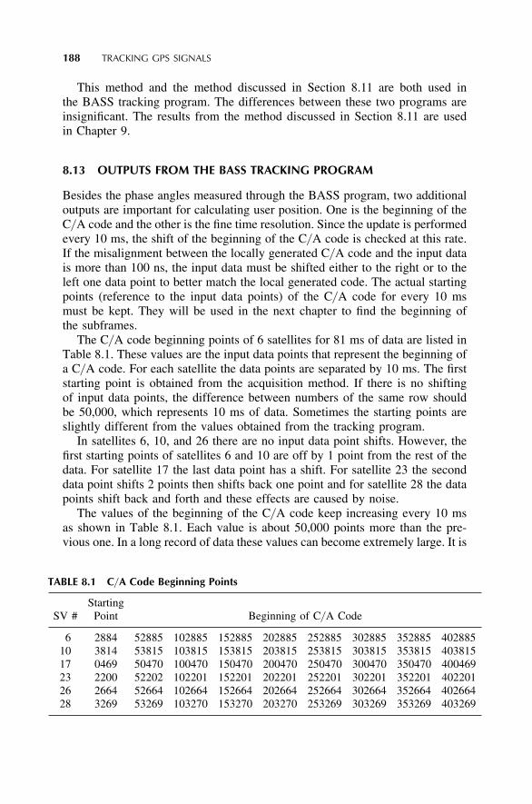
The C/ A code beginning points of 6 satellites for 81 ms of data are listed inTable 8.1. These values are the input data points that represent the beginning ofa C/ A code. For each satellite the data points are separated by 10 ms. The firststarting point is obtained from the acquisition method. If there is no shiftingof input data points, the difference between numbers of the same row shouldbe 50,000, which represents 10 ms of data. Sometimes the starting points areslightly different from the values obtained from the tracking program.

In satellites 6, 10, and 26 there are no input data point shifts. However, thefirst starting points of satellites 6 and 10 are off by 1 point from the rest of thedata. For satellite 17 the last data point has a shift. For satellite 23 the seconddata point shifts 2 points then shifts back one point and for satellite 28 the datapoints shift back and forth and these effects are caused by noise.

The values of the beginning of the C/ A code keep increasing every 10 msas shown in Table 8.1. Each value is about 50,000 points more than the pre-vious one. In a long record of data these values can become extremely large. It is

TABLE 8.1 C/ A Code Beginning Points

StartingSV # Point Beginning of C/ A Code

6 2884 52885 102885 152885 202885 252885 302885 352885 40288510 3814 53815 103815 153815 203815 253815 303815 353815 40381517 0469 50470 100470 150470 200470 250470 300470 350470 40046923 2200 52202 102201 152201 202201 252201 302201 352201 40220126 2664 52664 102664 152664 202664 252664 302664 352664 40266428 3269 53269 103270 153270 203270 253269 303269 353269 403269

8.14 COMBINING RF AND C/ A CODE 189

inconvenient to store these values. However, these values need not be so large.The reason for keeping these large values is easier to explain in the next chapter.In actual programming these values are kept between 1 and 5,000. For example,the beginning of the C/ A code for satellite 6 will have the same value of 2,885instead of the values listed in the table. The beginning of the C/ A code is usedto find the beginning of the subframes, which can be located within 1 ms ofinput data. This topic will be discussed in the next chapter. Since within 1 msthe beginning of the C/ A code is from 1 to 5,000, a value within this range issufficient to locate the beginning of the first subframe.

The time resolution in the above data is 200 ns, determined by the samplingfrequency of 5 MHz, thus, the beginning of the C/ A code can be measured withthis time resolution. With each value of the beginning of the C/ A code there isa fine time x calculated by Equations (8.45) or (8.49), which is not included inTable 8.1. These fine times can be used to improve the overall time resolution.

8.14 COMBINING RF AND C/ A CODE

In Sections 8.8 to 8.12 the BASS tracking method is discussed. In order to trackthe input signals for each satellite, two quantities are locally generated: a complexRF frequency and the C/ A code. Once the C/ A is generated, it is used all the time.The locally generated complex RF signal is updated at most every 10 ms becausethe carrier frequency changes very slowly for a stationary receiver as discussedin Chapter 3. The locally generated C/ A code and RF signal can correlate withthe input signal simultaneously. One convenient approach is to combine the C/ Acode and the Rf signal through point-by-point multiplication to generate a newcode. This new code can be used as the prompt code. This prompt code is shiftedtwo data points to the left and right to obtain the early and late codes. These threecodes consisting of the C/ A code and RF signals are used to correlate with theinput signal. The phase of the RF in the prompt signal is important because it isused to find the fine frequency and the phase transition in the navigation data. Theamplitudes of the early and late codes are used only to determine the fine time res-olution; therefore, the phase of RF signals in the early and late codes is not impor-tant. The fine frequency is calculated from Equation (8.42) and the new frequencyis used in generating the local RF signal for the next 10 ms of data. The phase dis-continuity in the Kernel function must be calculated and necessary adjustmentsmust be made as discussed in Section 8.9.

The outputs from the BASS method are the phase angles obtained fromthe prompt code. The phase angles are calculated every millisecond. After thephase adjustment discussed in Section 8.9, the phase should either be contin-uous between two milliseconds of data or changing by p. The absolute valuesof the phase angle are not very important because it depends on the initial sam-pling point. The difference angle is defined as the phase difference between twoadjacent milliseconds. If the difference angle is within ±p/ 2, it is considered asno phase shift. If the difference is outside the range of ±p/ 2, there is a p phaseshift. The p phase shift should happen in multiples of 20 ms.


8.15 TRACKING OF LONGER DATA AND FIRST PHASE TRANSITION

The BASS tracking program discussed in this chapter is based on tracking1 ms of input data. If the signal is weak, it is possible to track more than 1 msof data to improve sensitivity. It seems that the maximum data length that canbe tracked coherently is 20 ms without very sophisticated processing becausethe navigation data is 20 ms long. The input data must be properly selectedand there should not be a phase transition within the selected 20 ms of data.Under this condition, the sensitivity is improved by 13 dB (10 log (20/ 1)) overtracking 1 ms of data. If the data length is longer than 20 ms, it may contain aphase transition due to the navigation data. The phase transition will disturb theoperation of the tracking program. If multiples of 20 ms of data are used, thetracking process must cover all the possible combinations of phase transition.The tracking program can be rather complicated and calculation intensive.

In order to track 20 ms of data without a navigation data phase transition,one must find a phase transition in the data. This requirement puts an additionalrestraint on the acquisition program. The acquisition is not only required to findthe beginning of the C/ A code and the carrier frequency, it must also find aphase transition. If the phase transition cannot be found, it is impractical to track20 ms of data. Therefore, finding the phase transition becomes an importantrequirement to process weak signals.

8.16 SUMMARY

In this chapter the concept of tracking a GPS signal is discussed. Twoapproaches are presented: the conventional and the BASS methods. A generaldiscussion on the conventional phase-locked loop is presented and its applica-tion to GPS receiver is discussed. In addition, a BASS method is presented indetail. This method needs to generate the C/ A code only once; thus it may savecalculation time for software receiver design. Theoretically, the BASS methodat worst case may lose about 1 dB of sensitivity with 5 MHz sampling rate dueto the potential misalignment between the input signal and the locally gener-ated signal. Two methods of generating fine time resolution are discussed. Theoutputs from the tracking are also discussed. These outputs will be used in thenext chapter to find the user position.

APPENDIX(10)

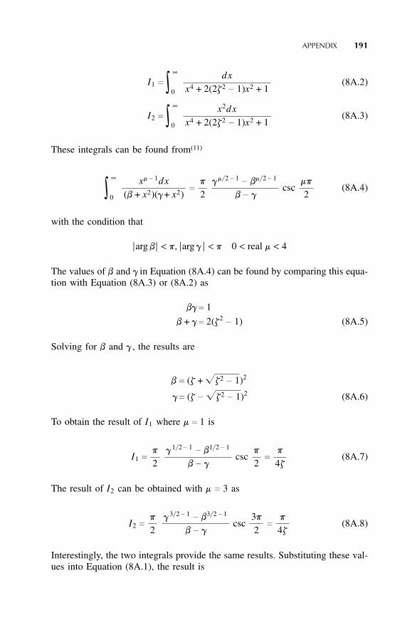
Equation (8.26) can be written as

Bn c qn

2p ∫∞

0

1 + 4z2xx4 + 2(2z2 − 1)x + 1

dx c qn

2pI1 +

qn

2p4z2I2 (8A.1)

where

APPENDIX 191

I1 c ∫∞

0

dxx4 + 2(2z2 − 1)x2 + 1

(8A.2)

I2 c ∫∞

0

x2dxx4 + 2(2z2 − 1)x2 + 1

(8A.3)

These integrals can be found from(11)

∫∞

0

xm − 1dx(b + x2)(g+ x2)

c p

2gm/ 2 − 1 − bm/ 2 − 1

b − gcsc

mp

2(8A.4)

with the condition that

|arg b | < p, | arg g | < p 0 < real m < 4

The values of b and g in Equation (8A.4) can be found by comparing this equa-tion with Equation (8A.3) or (8A.2) as

bgc 1

b + gc 2(z2 − 1) (8A.5)

Solving for b and g, the results are

b c (z +f

z2 − 1)2

gc (z − fz2 − 1)2 (8A.6)

To obtain the result of I1 where m c 1 is

I1 c p

2g1/ 2 − 1 − b1/ 2 − 1

b − gcsc

p

2c p

4z(8A.7)

The result of I2 can be obtained with m c 3 as

I2 c p

2g3/ 2 − 1 − b3/ 2 − 1

b − gcsc

3p

2c p

4z(8A.8)

Interestingly, the two integrals provide the same results. Substituting these val-ues into Equation (8A.1), the result is


Bn c qn

2 �z +14z � (8A.9)

which is the desired result.

REFERENCES

1. Gardner, F. M., Phaselock Techniques, 2nd ed., Wiley, New York, 1979.2. Best, R. E., Phase-locked Loops, Theory, Design, and Applications, McGraw-Hill,

New York, 1984.3. Stremler, F. G., Introduction to Communications Systems, 2nd ed., Addison-Wesley,

Reading, MA, 1982.4. Ziemer, R. E., Peterson, R. L., Digital Communications and Spread Spectrum System,

p. 265, Macmillan, New York, 1985.5. Chung, B. Y., Chien, C., Samueli, H., Jain, R., “Performance analysis of an all-digital

BPSK direct-sequence spread-spectrum IF receiver architecture,” IEEE Journal ofSelected Areas in Communications, vol. 11, no. 7, pp. 1096–1107, September 1993.

6. Van Dierendonck, A. J., “GPS receivers,” Chapter 8 in Parkinson, B. W., Spilker,J. J. Jr., Global Positioning System: Theory and Applications, vols. 1 and 2, AmericanInstitute of Aeronautics and Astronautics, 370 L’Enfant Promenade, SW, Washing-ton, DC, 1996.

7. Stockmaster, M. H., Rockwell Collins, Cedar Rapids, IA, private communication.1997.

8. Tsui, J. B. Y., Stockmaster, M. H., Akos, D. M., “Block adjustment of synchronizingsignal (BASS) for global positioning system (GPS) receiver signal processing,” IONGPS 1997 Symposium, pp. 637–643, Kansas City, MO, September 15–19, 1997.

9. Tsui, J. B. Y., Digital Techniques for Wideband Receivers, Chapter 10 of this book,Artech House, Norwood, MA, 1995.

10. Yu, J. S., West Virginia Instiute of Technology, private communication.11. Gradshteyn, I. S., Ryzhik, I. M., Table of Integrals, Series and Products, Equation

3.264-2, p. 300, Academic Press, New York, 1980.

Date post:	12-Feb-2022
Category:	Documents
Upload:	others
View:	14 times
Download:	0 times

Tracking GPS Signals

Documents