Tracking sperm whales with a towed acoustic vector sensor

Tracking sperm whales with a towed acoustic vector sensorAaron Thode,a� Jeff Skinner, Pam Scott, and Jeremy RoswellMarine Physical Laboratory, Scripps Institution of Oceanography, San Diego, California 92093-0205

Janice StraleyUniversity of Alaska Southeast Sitka Campus, 1332 Seward Ave., Sitka, Alaska 99835

Kendall FolkertP.O. Box 6497, Sitka, Alaska 99835

�Received 20 May 2010; revised 9 September 2010; accepted 13 September 2010�

Passive acoustic towed linear arrays are increasingly used to detect marine mammal sounds duringmobile anthropogenic activities. However, these arrays cannot resolve between signals arriving fromthe port or starboard without vessel course changes or multiple cable deployments, and theirperformance is degraded by vessel self-noise and non-acoustic mechanical vibration. In principleacoustic vector sensors can resolve these directional ambiguities, as well as flag the presence ofnon-acoustic contamination, provided that the vibration-sensitive sensors can be successfullyintegrated into compact tow modules. Here a vector sensor module attached to the end of a 800 mtowed array is used to detect and localize 1813 sperm whale “clicks” off the coast of Sitka, AK.Three methods were used to identify frequency regimes relatively free of non-acoustic noisecontamination, and then the active intensity �propagating energy� of the signal was computedbetween 4–10 kHz along three orthogonal directions, providing unambiguous bearing estimates oftwo sperm whales over time. These bearing estimates are consistent with those obtained viaconventional methods, but the standard deviations of the vector sensor bearing estimates are twicethose of the conventionally-derived bearings. The resolved ambiguities of the bearings deducedfrom vessel course changes match the vector sensor predictions.© 2010 Acoustical Society of America. �DOI: 10.1121/1.3495945�

PACS number�s�: 43.30.Sf, 43.30.Wi, 43.60.Fg, 43.60.Cg �WWA� Pages: 2681–2694

I. INTRODUCTION

Using a towed passive acoustic array to detect biologicsounds is a mature marine mammal monitoring and mitiga-tion method �Leaper et al., 1992�, with several commercialservices available for mitigation monitoring in the presenceof mobile anthropogenic activities such as seismic surveys. Atypical towed system consists of a collection of omnidirec-tional hydrophones that are sensitive to acoustic pressure.Estimating the directionality of the sounds is of considerablepractical importance for most mitigation applications, in thatthe location of marine mammals relative to noise-makingactivities may determine whether that activity must be sus-pended or even completely stopped. One hydrophone, byitself, cannot provide information about a sound’s direction;however, by spatially separating the hydrophones along thearray cable, the resulting signals can be beamformed to de-termine some information about signal directionality. For ex-ample, the simplest type of beamforming measures the rela-tive arrival time of a signal between two hydrophones; e.g.,�Gordon, 1987; Leaper et al., 1992; Gillespie, 1997; Barlowand Taylor, 2005�. If the signal arrives first on the hydro-phone closest to the tow vessel, then the signal must be ar-riving from roughly ahead of the hydrophones. Standard

a�Author to whom correspondence should be addressed. Electronic mail:
[email protected]
J. Acoust. Soc. Am. 128 �5�, November 2010 0001-4966/2010/128�5

Downloaded 13 May 2013 to 129.173.72.87. Redistribution subj

towed array systems typically use multiple hydrophonesseparated by a few meters along the tow cable to estimatesignal bearings.

However, while using spatially distributed hydrophonesto determine the direction of a sound is a standard procedure,the technique suffers from several disadvantages. First, theresolution of the direction measurement is frequency-dependent. For a given hydrophone spacing, a low-frequencysignal will have a less precise bearing than a high frequency-signal. However, if the frequency of a narrowband signal ishigh enough that its associated half-wavelength is smallerthan the array spacing, then the signal will appear to arrivefrom multiple directions, a phenomenon known as spatialaliasing �DeFatta et al., 1988�. Fortunately, many marinemammal signals are sufficiently broadband to avoid spatialaliasing issues �Miller and Tyack, 1998; Thode et al., 2000�.

A second disadvantage of standard single-cable towedarray systems is that directional measurements are less pre-cise along the “endfire,” or on-axis directions of the array,than along the “broadside” directions of the array. Thus get-ting precise bearings of sounds generated forward of the towvessel is impractical, an unfortunate situation given that thepositions of animals ahead of a vessel tend to be of highinterest to mitigation observers. Another challenge towed ar-ray systems face is noise contamination. Towed arrays areoften deployed less than a kilometer from the towing vessel.Even if the tow vessel is not the source of the mitigated
noise, the noise generated by the vessel itself can easily wash
© 2010 Acoustical Society of America 2681�/2681/14/$25.00

ect to ASA license or copyright; see http://asadl.org/terms

out other signals recorded on the array. Tow vessels availablefor mitigation monitoring are often not designed to minimizeacoustic noise, and thus engine harmonics and propellercavitations can easily mask most marine mammal sounds inthe vicinity. While direct engine noise is often restricted to afrequency band of a few hundred hertz, the oscillation ofunderwater bubbles produced by cavitation can easily extendinto the kilohertz range.

A final disadvantage of standard towed arrays is that atowed array system comprised of hydrophones distributedalong a single cable cannot distinguish between an acousticsignal arriving from port or starboard of the towing vessel. Asignal arriving from the port will produce exactly the samerelative arrival times across the hydrophones as would amirror-image signal arriving from the starboard. The “hand-edness” of a signal is defined here as the side from which anacoustic signal is arriving on a towed array. Thus a signal, orbearing derived from that signal, will have either a port orstarboard handedness.

This last weakness is a particular disadvantage for seis-mic surveys, which tend to raster a vessel back and forthover a fixed area. Were a seismic vessel able to determinefrom which side marine mammal acoustic activity is occur-ring, it could conceivably adjust its rastering pattern to moveaway from the animals, instead of shutting down completely.

Three methods have traditionally been used to resolvethis bearing ambiguity. A standard technique is to change thecourse of a vessel while a marine mammal is producing asequence of sounds, and then observe how the acoustic bear-ings of the sound sequence shift over time. If the vesseladjusts course such that the animal’s relative azimuth shiftstoward the bow, then the acoustic bearings would shift to-ward the bow. However, if the course shift orients the vesselfurther away from the animal, then the bearings will shifttoward the stern �Barlow and Taylor, 2005�. This tried-and-true technique is used here to independently verify the hand-edness of whale sounds. However, altering the course of avessel is a slow and often undesirable action �as is the casewith seismic vessels�, and the technique also fails if the sameanimal fails to make sounds before and after the vessel’scourse change.

A second technique is to deploy additional linear towedhydrophones such that their complete underwater spatial dis-tribution occupies a two-dimensional space rather than just aone-dimensional line. This approach is expensive and createsadditional logistic challenges of deployment, operation, andrecovery. A final method for resolving bearing ambiguities isto build a small three-dimensional assembly of hydrophoneson the tow cable, either as a ring around the cable or as asmall cage at the end of the cable.

This paper examines a fourth approach: incorporating anunderwater acoustic vector sensor �D’Spain et al., 1991a;1991b; D’Spain et al., 2006� into a linear towed array, inorder to provide unambiguous bearings to marine mammalsignals. Vector sensors have the ability to measure not onlyacoustic pressure, but also acoustic particle velocity. Sincethe latter is a vector quantity, such sensors have an inherentability to provide unambiguous bearings to a sound source,
at a frequency-independent resolution greater than provided
2682 J. Acoust. Soc. Am., Vol. 128, No. 5, November 2010


by a set of spatially distributed hydrophones, provided thatthe signal-to-noise ratio �SNR� of the signal is adequate�Greene et al., 2004; McDonald, 2004�. As will be discussed,for low SNR signal the vector sensors have to process thedata in such a way that substantially degrades the angularresolution. The vector sensor also provides noise-suppressioncapabilities unavailable to standard arrays, as well as tech-niques for identifying the presence of non-acoustic sourcesof noise contamination.

Section II of this paper reviews vector sensor processingtheory, with an emphasis on so-called “intensity processing”in the frequency domain, an approach that provides high res-olution bearing estimates for high SNR signals with minimalcomputational effort. This section also defines metrics fordetecting the presence of non-acoustic noise in the sensordata, as well as characterizing the spatial heterogeneity of thereceived acoustic field. Section III then describes the equip-ment used in the effort, including the vector sensor, the en-closing tow module, and the complete towed array system.Section IV describes the experimental effort, deployed froma fishing vessel in U.S. waters off the coast of Sitka, AK.Finally, Sec. V characterizes the noise performance of thearray, and demonstrates the sensor’s ability to detect andtrack sperm whale sounds unambiguously, even in the pres-ence of a noisy tow vessel. A side benefit of the vector sensorprocessing is an enhanced capability to identify the presenceof non-acoustic noise contamination in the towed array data.

II. THEORY

A. Basic concepts and geometric configuration

The mathematical description of the propagation of anacoustic wave through a fluid medium arises from the conti-nuity equation and Euler’s equation �Newton’s second law�:

�0�x�� v�x,t�

�t+ �p�x,t� = 0, �1a�

�p�x,t��t

+ ��x� � • v�x,t� = 0. �1b�

Here p�x , t� is the acoustic �perturbed� pressure, v is theacoustic particle velocity, �0 is the ambient fluid density, and� is the adiabatic incompressibility, which is equal to �0c2,where c= ��p /��S is the characteristic sound speed of themedium. Note that p is a scalar and v is a vector quantity, sothe acoustic field is characterized by four components. Alsonote that from Eq. �1a� a measurement of v is proportional tothe spatial gradient of acoustic pressure p. Thus a measure-ment of both p and v at a single point in space provides thesame information as a dense cluster of pressure measure-ments around that point, by applying a Taylor expansion�D’Spain, 1990; D’Spain et al., 1991a�.

These two first-order equations can be combined to forma wave equation with respect to pressure, or other scalarquantities such as acoustic and displacement potential�Jensen et al., 1994�. The simplest non-trivial mathematicalsolution to the wave equation is a propagating plane wave in
an infinite medium. Under these idealized circumstances the
Thode et al.: Sperm whale vector sensor tracking


acoustic velocity is proportional and in phase with the acous-tic pressure: �v�= p /�c. Therefore the time-averaged intensity�power flux� of the wave, which is a vector quantity �pv�,becomes ��p�2 /�0c2�s, where s is a unit vector pointing in thedirection of propagation. In this specific case the measure-ment of acoustic pressure with a hydrophone would be suf-ficient for characterizing the complete field intensity. How-ever, in general, independent measurements of both theparticle velocity and pressure field are required to obtain thetrue acoustic intensity, even in relatively simple cases such asan acoustic wave reflecting from a boundary �Chapman,2008�.

Suppose a situation exists where all four components ofan acoustic field have been measured by a sensor at a fixedpoint corresponding to the origin of the unprimed coordinatesystem in Fig. 1�a�. In this coordinate system the z-axis liesparallel to the ocean surface and points away from the tow-ing vessel, the x-axis points upward, normal to the plane ofthe ocean surface, and the direction of the y-axis points port,as defined by the right-handed coordinate system. The longaxis of the sensor is pitched � degrees relative to the z-axis,and the angular origin of the sensor is rotated � degrees withrespect to the x-z plane. Let v� be the velocity componentsof the acoustic field measured in terms of the primed axesindicated in Fig. 1�a�, representing the sensor’s frame of ref-erence. The corresponding particle velocity components inthe earth-based frame can be derived with two matrix rota-tions:

v = �cos � 0 − sin �

0 0 0

sin � 0 cos �� cos � − sin � 0

0 0 0

sin � cos � 0�v�. �2�

Once the velocity components are rotated into the desiredframe of reference, a complete description of the acousticwave �pressure and velocity� can be arranged into a time-dependent four-component vector A�x , t�= �p,vx ,vy ,vz�,with Ai�t� representing the ith element of the vector at time t.

y

z

x

α

θ

y

x

z

z

x

η

φ

γ

y

β

a) b)

c)

z’

x’

y’

FIG. 1. �Color online� Geometry of towed vector sensor. �a� Relationshipbetween the sensor frame of reference �primed axes� and the earth-basedframe of reference �unprimed axes�. �b� Definitions of acoustic bearing �,elevation �, and azimuth �. �c� Definition of acoustic roll angle �. A positivevalue of � indicates energy arriving from the starboard side of the towedarray.

Thus A1= p, A2=vx and so on. Note that A, unlike v, is not

J. Acoust. Soc. Am., Vol. 128, No. 5, November 2010


a contravariant vector, as p is constant under a coordinaterotation.

B. Additive beamforming vs. vector intensityprocessing

Assume that the acoustic field is dominated by a com-pact deterministic source arriving from an azimuth � andelevation angle � in the earth-based reference frame �Fig.1�b��. Although redundant, it is also convenient to define twoadditional angles: a roll angle � that is negative if the signalis arriving from port and positive if arriving from starboard�Fig. 1�c��; and an “acoustic bearing” �, which indicates theangle between the array cable �negative z-axis� and the in-coming signal.

Two techniques exist for determining the directionalityof the field given particle velocity information: “additivebeamforming” and “vector intensity processing.” In additivebeamforming �McDonald, 2004; D’Spain et al., 2006� thecomponents of A are weighted and summed in a manneridentical to conventional beamforming methods:

D��,�,t� = a0p�t� + �j=1

3

aj�0cv j�t�cos�� j� ,

cos��1� = sin �, cos��2� = sin � cos � ,

cos��3� = cos � cos � , �3�

where aj are normalization factors and cos�� j� are directionalweights that are the cosines of the angles between each can-didate look direction and each axis.

In essence the additive approach is a series of hypothesistests, where every possible combination of � and � must besystematically tested using Eq. �3�, which is maximized atthe correct values of these angles. Note that the acousticvector data allow the arriving signal directionality to be fac-tored into the angles � and �, whereas conventional time-delay beamforming can only provide the acoustic bearing �.

Using concepts from information theory it can be shownthat additive beamforming is the optimal approach for detec-tion of weak, low SNR signals �Brown and Rowlands, 1959;D’Spain et al., 2006�, and in theory can provide an increaseof 6 dB in the signal-to-noise ratio. This approach is also thealgorithm used in Navy DIFAR sonobuoys �1983�. However,the additive approach is also computationally intensive, be-cause Eq. �3� must be computed for every candidate lookdirection.

A much faster, physics-based approach for estimatingsignal direction is available if a signal has sufficiently largeSNR to obviate detection concerns �D’Spain et al., 1991b;1991a; Greene et al., 2004�. In vector intensity processing

the ensemble-averaged acoustic intensity Ji�x , t�� ji�x , t��= �p�x , t�vi�x , t�� is computed along each coordinate axis. Thetime-averaged acoustic intensity is unambiguous with re-spect to direction; for example, two plane waves propagatingin opposite directions will have opposite signs in their acous-
tic intensity measurements.
Thode et al.: Sperm whale vector sensor tracking 2683


As this vector points in the direction of energy flow, theazimuth, elevation, and acoustic bearing � can be directlyinferred from the relative magnitudes of the intensity com-ponents along each coordinate axis:

tan�� = − Jy/Jz, �4a�

tan�� = Jx/Jy2 + Jz

2, �4b�

cos�� = − Jz/Jy2 + Jx

2, �4c�

tan�� = − Jy/Jx. �4d�

The sign of � indicates the handedness of the signal.

C. Estimating bearing and handedness in thefrequency domain

While the acoustic intensity Ji can be band-pass filteredin the time domain and then applied to Eq. �4�, processingthe acoustic intensity in the frequency domain provides a keyadvantage: it yields several metrics for signal quality thathelp determine the most effective bandwidth to use whencomputing bearings. These metrics provide insight into boththe spatial heterogeneity of the acoustic ambient noise field,as well as the presence of non-acoustic noise contaminationin the vector sensor data �D’Spain et al., 2006�.

Let A�x ,� be the vector consisting of the Fourier trans-forms of the corresponding band-limited time series inA�x , t�. Then via Parseval’s theorem

�Ai�t�Aj�t�� = �0

Ai�t�Aj�t�dt = �1

2

Ai��Aj��d

�1

2

Sij��d . �5�

The ergodicity assumption has been used to obtain the sec-ond term. The components of Sij can be arranged into across-spectral density matrix S, the ensemble averaged outerproduct of the vector A�x ,�, which in turn can be decom-posed into real and imaginary components: S�x ,�=C�x ,�+ iQ�x ,�. Under the ergodicity assumption, suc-cessive time “snapshots” of the outer products of A�x ,� canbe averaged to estimate S. The various components of thematrix can be interpreted as physical quantities related toacoustic power flow. Of particular interest here are the off-diagonal components S1i, which correspond to the cross-spectra between the pressure and various particle velocitycomponents. The real parts of these cross-spectra, C1i�x ,�,labeled the active intensity, arise from the in-phase compo-nents of the pressure and velocity, and thus relate to the netpower being propagated through the space by the acousticfield. The imaginary components of the pressure-velocitycross spectra, Q1i�x ,�, labeled the reactive intensity, relatethe components of the pressure and velocity that are 90° outof phase, corresponding to the power flow required to sup-port spatial heterogeneity in the acoustic field �D’Spain,1990�. For example, in a three-dimensional plane wave thepressure and velocity are completely in phase, and all the
energy in the field is transported in the direction of propaga-


tion. The reactive intensity is thus zero, reflecting the factthat a plane wave is spatially homogenous. By contrast aspherically expanding wave and a plane wave reflecting froma plane boundary both contain spatial heterogeneity, so aportion of the energy in the acoustic wave must be investedin maintaining this structure, and consequently the reactiveintensity is nonzero �Fletcher, 1992�.

In exact analogy with Eq. �4� the various angular direc-tions can be computed from the components of the activeintensity:

tan�� = − C13/C14, �6a�

tan�� = C12/C132 + C14

2 , �6b�

cos�� = − C14/C132 + C12

2 , �6c�

tan�� = − C13/C12, �6d�

where C1j =�1

2C1j��d is the band-integrated value of theactive intensity along axis j.

D. Estimating non-acoustic noise contamination onsensor

The reactive intensity Q, although not directly involvedin bearing estimation, provides useful information about thenature of the acoustic and non-acoustic components of thedetected signal. For the case where the vector sensor dataarise purely from acoustic signals, the scaled ratio of thereactive intensity to the acoustic pressure autospectrum pro-vides information about the spatial gradient of the acousticfield at a given frequency �Eq. �29� in D’Spain et al.,1991a�:

Rj�� 0c0Q1j��

C11��= −

1

4�

�C11��C11�� xj

� . �7�

Specifically, this “reactive ratio” Rj�� yields the fractionalchange in the pressure autospectrum arising from a fractionalchange in position along the xj direction, relative to anacoustic wavelength. If portions of signal dominated byacoustic power are sampled over time, then the distributionof the resulting set of Rj measurements at a given frequencywould be expected to cluster around well-defined peak, pro-vided that the spatial statistics of either the acoustic source oracoustic ambient noise background at that frequency remainstationary over time. A low mean value of Rj�� would in-dicate that the acoustic field at that frequency is relativelyspatially homogenous, and dominated by the active intensity.A large nonzero value of Rj at a particular frequency doesnot mean that the frequency component cannot be used to

estimate C1j, but does suggest that only a small fraction ofthe signal power would actually contribute to that estimate.

By contrast, a signal frequency contaminated by randomelectrical noise or stochastic mechanical vibrations, uncorre-lated across channels, would be expected to yield randomrelationships between the phase of the pressure and velocitycomponents of the vector sensor measurement. Therefore,
the distribution of Rj, derived from large numbers of con-


taminated samples over time, would be nearly uniform orotherwise display no clear clustering around a mean value.Plotting this distribution can thus provide one indication ofthe relative contributions of non-acoustic noise over the vec-tor sensor acoustic spectrum. This approach would not flagcorrelated electrical or mechanical interference across allsensor channels.

Other metrics characterizing non-acoustic noise con-tamination can be derived, exploiting the fact that the basicequations of acoustic propagation place constraints on therelationships between the components of the cross-spectralmatrix S. A second potential diagnostic arises from the fol-lowing second-order property of acoustic intensity �D’Spainet al., 2006�:

�S11�� − ��c�2�j=2

4

Sjj�� = �j=2

4�Q1j

�xj. �8a�

In vector sensor measurements dominated by an acousticfield with little spatial heterogeneity, Eq. �7� indicates thatthe levels of the reactive intensity Q will be small and spa-tially uniform, and under such circumstances it has been pos-tulated that the right-hand side of Eq. �8a� will be approxi-mately zero, so the scaled pressure autospectrum �S11�should equal the scaled sum of the three velocity autospectra�D’Spain et al., 2006�. Stated more succinctly, a spatiallyhomogenous acoustic field should statistically divide its en-ergy equally between kinetic and potential forms, so an im-balance between these components may indicate the pres-ence non-acoustic contamination. A metric M1 can bedefined for evaluating this energy balance:

M1

��c�2�j=2

4

Sjj�� − S11��

��c�2�j=2

4

Sjj�� + S11��

. �8b�

If the reactive ratios derived from large numbers of datasamples cluster around zero, then corresponding values ofM1 substantially different from zero may flag non-acousticsignal contamination.

A final potential test for non-acoustic contaminationarises from a relationship between the cross spectra of theparticle velocity components and the active and reactiveacoustic intensity vectors:

�Q34��,Q42��,Q23�� =C1�2,3,4�� Q1�2,3,4��

S11��.

�9a�

Here the notation X1�2,3,4� represents the submatrix compo-nents �X12,X13,X14� of matrix X, arranged as a vector, and‘x’ is the vector cross product. The left side of Eq. �9a�encapsulates the degree of coherence between the compo-nents of acoustic particle velocity—a measure of particlemotion polarization. A second metric M2j can then be defined
such that


M21 =

�Q34�� − � C1�2,3,4�� Q1�2,3,4��

S11��

x�

�Q34�� + � C1�2,3,4�� Q1�2,3,4��

S11��

x� ,

M22 =

�Q42�� − � C1�2,3,4�� Q1�2,3,4��

S11��

y�

�Q42�� + � C1�2,3,4�� Q1�2,3,4��

S11��

y� , . . . .

�9b�

Unlike Eq. �8a�, Eq. �9b� does not require that a set of reac-tive ratio measurements Rj cluster around zero in order to bevalid. Thus values of M2j that diverge significantly from zeromay be a more robust flag of non-acoustic contaminationthan M1.

In Sec. V plots of the distributions of Rj, M1 and M2j ofboth sperm whale and ambient noise data are used to deter-

mine the appropriate bandwidth over which to compute C1j

and Eq. �6� for transient sperm whale clicks.

III. EQUIPMENT

A. Vector sensor module

The vector sensor used in this effort is the Meggitt-Wilcoxon VS-205. Acoustic vector sensors are not a noveltechnology; for example, the United States Navy has used aDIFAR �Directional Finding And Ranging� sonobuoy for de-cades �Naval Weapons Support Center, 1983�. However, DI-FAR sensors are bandlimited to less than 4 kHz, can onlydetect particle velocity along two axes, are extremely sensi-tive to mechanical vibration, and are thus unsuited for de-ployment in towed array systems. However, in recent yearsthe development of new piezoelectric materials has led to thedevelopment of small, sensitive, and low-noise vector sen-sors that can measure particle acceleration from a towed ar-ray �Shipps and Deng, 2003�.

The cutoff frequency of the VS-205 is around 11 kHz, soin principle its useable range covers many marine mammalvocalizations, including baleen whale calls, sperm whale pul-sive signals, and large odontocete “whistles” �Richardson etal., 1995�. The sensor outputs consist of an omnidirectionalacoustic pressure signal and separate acoustic particle accel-eration components for each orthogonal spatial axis. Thesensor also incorporates instrumentation for measuring pitch,roll, and heading so that the sensor outputs can be rotated toa coordinate system aligned with the ship heading and thelocal vertical. In terms of the geometry of Fig. 1�a�, the sen-sor effectively outputs estimates of � and �.

Figure 2 shows how the vector sensor was incorporatedinto a compact tow module designed to minimize mechanicalvibration in the system, based on information released intothe public domain by the Naval Underwater Warfare Center�NUWC�. The 1.1 m length module consists of a 6.3 cmouter diameter polyurethane tube with. 63 cm wall thickness,filled with ISOPAR™ isoparaffinic fluid. Four KEVLAR
strength members span the length of the tube, connecting the


anodized aluminum ends together via a spacer at the tail end,which is mechanically attached to the tail cap via a threadedrod, permitting adjustments in the member tension. Thusdrag forces resulting from a stabilizing rope attached to theend cap would not risk pulling the module apart. Two fillvalves allow for bleeding air out of the system. The head caphas a void to accommodate interface electronics.

B. Towed array design

The vector sensor module is connected via a BratnerMINM-25 module connector to an 800 m towed array, com-prised of cable containing 20 twisted single pairs, manufac-tured by Falmat, Inc. A three-element linear hydrophone ar-ray with total aperture of 2.65 m sat 6.1 m meters ahead ofthe module, and a second three-element array of identicalspacing sat an additional 500 m further up along the cable.All array hydrophones have a flat response between 100 Hzand 35 kHz, and a sensitivity of �158 dB re 1 V /�Pa. Theacoustic data collected on the array hydrophones were usedto provide bearing estimates of marine mammal sounds us-ing standard time-of-arrival techniques, independent of thevector sensor measurements.

All acoustic data, including the vector sensor measure-ments, were transmitted via analog signal to a breakout boxon board the vessel, which then transferred the signal viabalanced audio cables to an ADAT HD-24 hard disk recorder,which sampled all acoustic data, including the vector sensor,at a 96 kHz sampling rate with 24 bit dynamic range. Duringreal-time operations, the outputs of the hard disk recorderwere then digitized using a MOTU Traveler input board, andwere then displayed using the bioacoustic software packageIshmael �Mellinger, 2002�. The non-acoustic sensors �NAS�transmitted their information digitally when polled once asecond by a LabView program. The low polling rate waschosen to minimize electrical interference to the analog datachannels. Each subarray had an integrated accelerometer andmagnetometer �Terella Inc.� that transmitted digital data on

FIG. 2. �Color online� Engineering drawing of towed array module, viewedlooking down the positive y-axis shown in Fig. 1. The towed array cableattaches to the far right.

pitch and roll, respectively, which were polled and logged by



vendor software on a laptop. The combined weight of thearray in water was approximately 40 kg, and the array couldbe towed at speeds up to six knots relative to the surroundwater. At six knots the sensor tows at around 30 m depth.

IV. PROCEDURE

A. Location

The vector sensor module was tested in July 2008 usingthe 19 m fishing vessel Cobra, in U.S. territorial waters nearSitka, AK, southwest of Kruzov Island. Sperm whales �Phy-seter macrocephalus� frequent deep waters in the Gulf ofAlaska, and have learned to recognize the sound of demersallongline fishing activity so that they can approach the vesselsto depredate the lines �Thode et al., 2007�. The continentalshelf is very narrow near Sitka, providing a convenient loca-tion where natural sperm whale habitat lay within U.S. terri-torial waters. Sperm whales produce broadband transientsounds called ‘clicks’, with bandwidth between 0.5 to over15 kHz at close ranges, and have durations on the order of5–15 ms, depending on the received signal-to-noise ratio�Worthington and Schevill, 1957; Watkins, 1977; Rice, 1989;Whitehead, 2003�.

B. Data collection

Whenever the fishing vessel entered water depths greaterthan 200 m, the array was deployed via a hydraulic winch offthe stern, while holding the vessel at a steady course of 4knots relative to the current. When the full length of cablehad been deployed, the winch was secured and a 10 m deckcable was attached to the front end of the array cable. Theother end of the array cable was then connected to the deckbox on the bridge. The entire array and vector sensor modulewere powered up, and the hydrophones of the rear subarraywere monitored aurally and visually via the software pro-gram Ishmael. All raw data were written to the ADAT harddisk recorder, and all NAS data were written to a laptop textfile. A simple real-time “energy” detector integrated the spec-tral power of an equalized spectrogram between 2 and 8 kHz,using a 512 point FFT window. Whenever this metric ex-ceeded a threshold value, the acoustic bearing � was com-puted using relative time-of-arrival measurements on two el-ements of the rear subarray.

Whenever sperm whale sounds were detected, the real-time acoustic bearings provided by the hydrophone arraywere used to guide the vessel toward the correct vicinity.Observers noted the times that the vessel course was ad-justed, as well as the direction �port or starboard� and theamounts of course change. By observing how the acousticbearings of sperm whale clicks shifted after the ship’s coursechanged, the vessel could be maneuvered toward the ani-mals.

C. Data analysis

After the field effort the acoustic bearings of spermwhales were computed using three different techniques.First, the rear subarray hydrophone data were completely
reprocessed using conventional time-of-arrival methods, pro-


ducing a complete time record of sperm whale acoustic bear-ings. The vector sensor data were then only used to resolvethe port/starboard ambiguity of the clicks. Second, the rearsubarray data were still used to detect sperm whale clicks,but then vector sensor data were used to derive bearing esti-mates via Eq. �6�. If a particular detection had been logged asbeing centered at time t and acoustic bearing �, then thevector sensor data were sampled centered at a time t+ �L /c��cos��, with L=6.1 m being the spatial separationbetween the rear subarray and the vector sensor, and c=1500 m /s. Finally, the vector sensor was used to both de-tect sperm whale sounds and estimate their acoustic bearings,using no information from the rest of the towed array system.

In the latter two cases 5 ms snippets of each click wereextracted from the four vector array analog channels. Esti-mates of the array roll � and pitch � were estimated for eachsnippet by averaging 10 s of the roll and pitch values beforeand after the time onset of the snippet. After projecting thetime series data into the earth-based reference frame usingEq. �2�, each snippet was subdivided into a set of 12 samplesegments overlapped by 90%, each Hanning windowed be-fore being subjected to the FFT.

For each discrete frequency i, the corresponding Fou-rier coefficients from the particle acceleration data were di-vided by −ii, converting the data units from particle accel-eration into particle velocity. The coefficients derived fromeach of the four channels were then arranged into the samplevector Aest, whose outer product then formed a snapshot ofthe cross-spectral density matrix Sest at that frequency, foreach 128-pt segment. Successive snapshots of Sest for agiven sperm whale click snippet were averaged together, andwere then used to derive Rj, M1, and M2j for each detectedsnippet as a function of frequency using Eqs. �7�–�9�. Whenthe distributions of all three metrics derived from all detectedclicks are plotted, an appropriate bandwidth for computingbearings was identified, and the active intensity Cest, the realpart of the time-averaged Sest, was integrated over this band

per Eq. �5�. The integrated active intensity C1j was then usedto estimate the acoustic bearing and roll angle of each clickvia Eq. �6�.

In addition to analyzing the sperm whale signals di-rectly, Eqs. �7�–�9� where also applied to 20 ms snippets ofdata collected 0.5 s before the onset of each sperm whaleclick, providing statistical samples of ambient noise condi-tions. The distribution of the three metrics from these datapermitted estimation of the ambient noise spatial gradientsand insight into non-acoustic contamination of the vectorsensor signal between 1 and 20 kHz.

V. RESULTS

A. Data set description

The first deployment of the vector sensor took place onJuly 20, 2008, without a stabilizing rope streamer attached tothe end of the module. The resulting motion of the modulewas unstable, with the measures of the roll �� fluctuating byover �90° over 20 s intervals. On July 21 the array wasredeployed at 08:53 local time, but now 10 m of 1.43 cm-
diameter line had been attached to the rear eyebolt of the


sensor module, and then an additional 10 m of 1.9 cm diam-eter line was attached to the first line, providing a total lengthof 20 m of stabilizing rope. The improvements of the arraydynamics are clearly seen in Fig. 3; the roll value fluctua-tions decreased to �30° over 20 s intervals.

At 09:12 sporadic and faint sperm whale sounds weredetected, but were difficult to track due to interfering vesselpulsive noise. Once bearings had been confirmed, the vesselbegan changing course at 9:53 to converge on the animals.The vessel master noticed another fishing vessel to the north-west off the port bow, and at 10:29 adjusted course to headdirectly toward the vessel. By 11 a.m. it was clear that twoanimals were present somewhere in the vicinity of this sec-ond fishing vessel, and over the next two hours the towingvessel made five course changes in an attempt to determinewhether the animals lay to the port and starboard. The vesselfirst shifted 50° to starboard, and by 11:34 the ambiguity ofone animal had been resolved. The vessel then turned anadditional 30° to port in order to head directly toward themore intense stream of clicks, in an attempt to obtain a visualsighting on at least one animal. Figure 4 displays spectro-grams of all vector sensor components at 11:53, a time whenthe sperm whale acoustic bearings approached closest to thearray broadside.

As the bearings began to shift toward the beam twoadditional port turns were made at 12:24 and 12:36, in anattempt to converge on the animal. At 14:06 the effort wasabandoned and the array gear recovered. Over 1813 clicksfrom two individual sperm whales had been recorded over5 h.

B. Signal quality analysis

Figure 5 plots the distribution densities NR,j�Rj ,� of thereactive ratios Rj�� extracted from all 1813 clicks as a func-tion of frequency between 1 and 20 kHz, along each axis inthe earth-based reference frame of Fig. 1�a�. The horizontalbin width is 0.1, and the distributions are normalized as adensity such that �−1

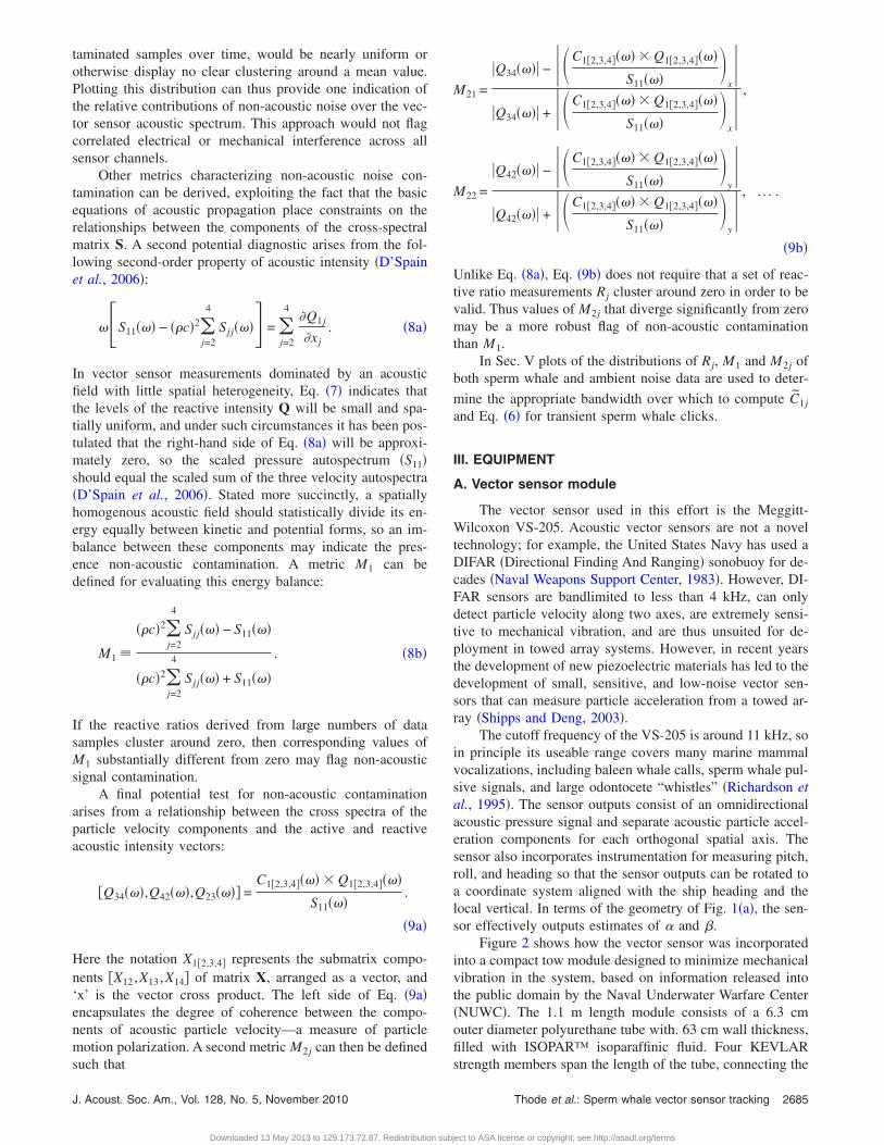
1 NR,j�Rj�dRj =1.Figures 6 and 7 show similarly normalized distributions

of the metric M1 and the three components of M2j, and thethree figures combined illustrate the features of these distri-butions under situations where the vector sensor signal isdominated by a high signal-to-noise ratio acoustic signal.The distributions of Rj and M2j between 4 and 10 kHz dis-played features characteristic of a clean acoustic signal, andthus that band was used for subsequent computations. Thedetails of the metric analyses are presented in Sec. VI.

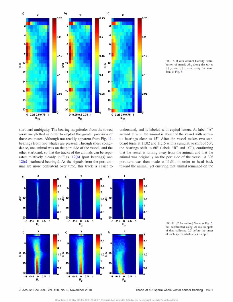
For comparison, Figs. 8–10 show the correspondingdensity distributions of Rj, M1, and M2j of background noisesnippets collected 0.5 s before the onset of each sperm whaleclick, thus providing opportunities to observe both the spatialstructure and potential non-acoustic signal characteristics ofthe vector sensor background data between 1 and 20 kHz.

C. Tracking results

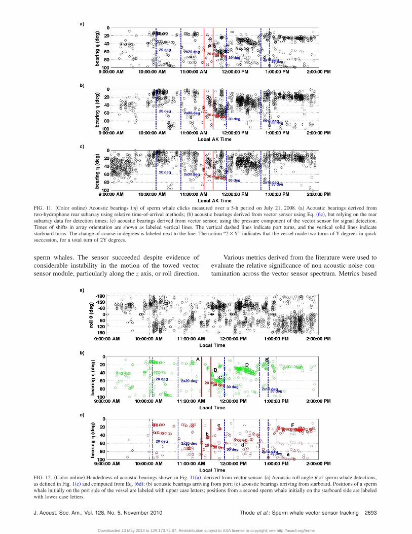
Figure 11 displays the 1813 acoustic bearings �� fromthe 5-h sequence, derived from the three approaches dis-
cussed in Sec. IV C, using signal components between 4 and


10 kHz. Figure 11�a� shows the bearings derived from con-ventional time-of-arrival processing on the rear subarray,without using the vector sensor. Figure 11�b� shows theacoustic bearings derived from vector sensor using Eq. �6c�,but still relying on the towed array data to detect the pres-ence of sperm whale clicks. Finally, Fig. 11�c� plots theacoustic bearings detected and estimated using the vectorsensor data only.

The times at which the towed vector sensor changedcourse are indicated by vertical lines; dashed lines representport turns, while solid lines indicate starboard turns. Thetime lag between when the vessel altered course and whenthe end of the towed array followed suit was estimated to beabout 12 min, or the 800 m length of the cable divided by thetypical vessel speed of 1 m/s �2 kn�.

Figure 12 shows how the vector sensor assigned theacoustic bearings to the port or starboard. Figure 12�a� dis-plays the acoustic roll angle � of the sperm whale clicks,derived by applying Eq. �6d� to the sperm whale data. Per thegeometry of Fig. 1�a�, a negative roll angle corresponds to anactive acoustic intensity arriving from the port side, and viceversa. The standard deviation of the roll estimates were com-puted over 10 s intervals, and over 80% of the deviations areless than �45°. Figures 12�b� and 12�c� take the acousticbearings derived from the towed array �Fig. 11�a��, and thenassign them to port and starboard locations, based on the sign
of �. To clarify the upcoming discussion, key sets of bearings


are labeled alphabetically, with upper-case labels ‘A’ through‘F’ associated with one whale track, and lower case labels ‘a’through ‘e’ associated with a second, fainter whale track.

VI. DISCUSSION

A. Signal quality analysis

Figures 5–7 illustrate metrics of the sperm whale clickquality as a function of frequency. During these times thevector sensor signal should be dominated by a transientacoustic signal with high levels relative to the backgroundlevels on the sensor, minimizing non-acoustic contamination.Thus the M metric distributions derived from the entire clickdata set are expected to be compact distributions close tozero over the frequency band of significant sperm whaleacoustic signal. Furthermore, as the acoustic signal is clearlyin the Fraunhofer �far-field� zone of the whale, and the vectorsensor is over 30 m below the ocean surface, the closestreflecting boundary, the propagating acoustic energy wouldbe expected to propagate as a 3-D plane wave, with theacoustic pressure and particle velocity completely in phase.As a consequence the reactive intensity matrix Q from eachclick should be zero, and the distribution of the Rj valuesderived from the clicks are expected to be compact distribu-tions clustering around zero.

The density distributions of the Rj in Fig. 5 indeed show

FIG. 3. �Color online� Mechanical dynamics of vectorsensor module, towed with a 20 m stabilizing rope,measured on July 21, 2008. The solid center line indi-cates the mean values extracted over 20 s of measure-ments, and the outer dashed lines indicate the standarddeviations of the measurements. �a� Vector sensor pitch��; �b� Vector sensor roll ��; �c� Vector sensor mag-netic heading.

values clustering close to zero along both the x and y axes



between 2 and 20 kHz. Below 2 kHz the distributions of R1

and R2 are nearly uniform between �2.5 and 2.5 �Figs. 5�a�and 5�b��, suggesting non-acoustic contamination in thisband. The clustering near zero at frequencies above 11 kHzmay be due, in part, to the fact that the sensitivity of thevector sensor to particle velocity motions decreases rapidlywith frequency in this band. Small values of particle velocitywould thus yield values near zero for all the metrics over thisrange.

More interesting is the observed distribution of R3, mea-sured along the z-axis, parallel with the array cable. Below 2kHz the distribution of the reactive ratios are nearly uniform,indicative of non-acoustic contamination. Between 4 and 10kHz the ratios do roughly cluster around zero, but then thescatter of the distribution widens considerably above 10 kHz,suggesting an increase in the relative contribution of non-acoustic noise factors. Therefore even though the spectro-grams in Fig. 4 clearly display sperm whale click compo-nents up to 15 kHz range, Fig. 5�f� suggests that the best-quality bandwidth for computing bearings lies below 10 kHz.

The M2j distributions in Fig. 7 reinforce the general im-

FIG. 4. �Color online� Spectrograms of spectral density for three seconds ofthe conventional hydrophone and vector sensor output on July 21, 2008,11:53:00, in terms of �a� pressure �conventional hydrophone�; �b� x axisparticle velocity; �c� y axis particle velocity; and �d� z axis particle velocity.The units of the pressure spectral density are in terms of dB re 1 �Pa2 /Hz.The time series of the original particle acceleration measurements wereconverted from gals to �Pa Hz by multiplying by �106��c. After computingthe resulting spectral densities, the densities were weighted by �2�f�−2 toconvert the units of images �b�–�d� into dB re 1 �Pa2 /Hz. Note the strongimpulsive contamination below 4 kHz in the plots �a� and �d�.

pressions created by the reactive ratio plots. The frequency



band between 2 and 3 kHz shows the metrics clustering atthe high end of the scale, albeit more weakly along the zaxis; reinforcing the impression that non-acoustic contamina-tion dominates the sperm whale data over this bandwidth.Between 4 and 10 kHz the data clusters near zero, indicatingthe presence of a strong acoustic signal, and then above 10kHz the distributions are either uniform or weakly clusternear 1. A strong non-acoustic component on the z axis chan-nel is visible at 13.5 kHz, a resonance frequency of the VS-205.

The performance of the M1 metric in Fig. 6 is disap-pointing, in that the distributions cluster around nonzero val-ues at all frequencies, including the promising 4–10 kHzband flagged by the previous two metrics. For a possibleexplanation, recall from Eq. �8� that the M1 metric is onlyvalid if the spatial gradient of the reactive intensity is zero;thus one possible explanation for the observed distributionsis that at least one component of the reactive intensity has asignificant spatial derivative. Another possible explanation isthat an imperfect calibration between the pressure and par-ticle velocity components that yields a specific acoustic im-pedance different from �c, although such an error would alsobe expected to affect the other metrics.

Figures 8–10 provide further insight into these metricsby plotting their distributions, derived from data sampleswhen sperm whale clicks are absent. The density distribu-tions of Rj shown in Fig. 8 indicate a significant reactiveintensity component in the background noise of the towedsensor. The R2 values along the y axis in Fig. 8�e� clusterclose to zero over most of the bandwidth, consistent withexpectations of a non-directional acoustic ambient noise fieldin the azimuthal �y-z� plane. However, the R1 values alongthe x axis cluster around �0.1. A small vertical spatial gra-dient in the ambient noise field is not surprising, presumingthat the primary mechanism behind the acoustic ambientnoise background was air-sea interactions at the ocean sur-face. Most noticeably, the R3 values along the z-axis clearlycluster around nonzero values above 5 kHz. The distribu-tions, while displaying some scatter, are clearly non-uniform,suggesting that the background noise along the z-axis arisesfrom acoustic noise with a fairly strong spatial gradient inthe direction of the towing vessel. The fishing vessel wascertainly noisy in terms of direct engine noise, hull vibration,and propeller cavitation; of the three, cavitation noise mightbe expected to be the most likely source of acoustic noiseabove 5 kHz.

The scatter in the distributions gradually grows quitelarge below 5 kHz, suggesting that non-acoustic contamina-tion steadily increases with decreasing frequency in the back-ground noise spectrum. The source of this contaminationseems directional, as the x and y components suffer muchless scatter than the z direction.

Figure 10, which plots the M2j metrics for the back-ground noise levels, reinforces the impression that the non-acoustic contributions to the background noise levels worsensignificantly below 5 kHz. Furthermore, the relatively poorclustering of the distributions at higher frequencies suggeststhat non-acoustic sources contribute non-trivial amounts of
background over a broad frequency range, when no sperm


whale sound is present. The nonlinear resonance response ofthe VS-205 at 13.5 kHz is clearly visible on all axes.

Figure 9, which plots the distributions of the M1 metricderived from the noise samples, shows no frequency rangewith values near zero, a result similar Fig. 6. As the results ofFig. 8�f� suggest that a strong spatial gradient exists in theacoustic field along the z axis, the most likely explanation forthe observed distribution of the M1 metric is that the assump-tions behind Eq. �8� are invalid, and this metric should not beused when evaluating appropriate bandwidths for bearing es-timation on a towed array system.

If the results of the M1 metric are ignored, then thedistributions of the reactive ratio and M2j metrics in Figs. 5

FIG. 6. �Color online� Density distribution of metric M1 plotted as a func-
tion of frequency, using the same data as Fig. 5.


and 7 imply that a frequency band between 4 and 10 kHz isa region with high relative active acoustic intensity and lownon-acoustic contamination during times when a sperm clickis present. Furthermore the distributions in Figs. 8 and 10also imply that in the absence of a high signal-to-noise ratioacoustic signal, the relative levels of non-acoustic noise con-tamination on the sensor increase steadily with decreasingfrequency, becoming dominant below 5 kHz. Based on thesecombined considerations, all bearing estimations discussedbelow are derived using sperm whale signal components be-tween 4 to 10 kHz.

B. Estimating bearing and signal handedness

A comparison between the acoustic bearings in Figs.11�a� and 11�b� shows that the time evolution of the acousticbearings estimated directly by the vector sensor is similar tothose obtained from the rear subarray, providing confidencethat the intensity-based processing has been implementedcorrectly, and that in principle a single sensor could replace adistributed array of hydrophones. However, the precision ofthe vector sensor acoustic bearing estimates is less precisethan those obtained through conventional time-of-arrivalmethods: the standard deviations of the vector sensor bearingestimates are �10°, vs. about �5° for the relative time-of-arrival methods applied to the rear subarray. One likely rea-son behind these larger deviations is the instability in thevector sensor physical roll angles �� displayed in Fig. 3�b�.Figure 11�c� shows the 1798 sperm whale clicks that thevector sensor detected directly, which was only 15 clicks lessthan what was detected by the standard towed array system.

Figure 12 replots the magnitudes of the bearings in Fig.

FIG. 5. �Color online� Density distri-bution of reactive ratio Rj along the �a�x; �b� y; and �c� z axis, derived from1813 sperm whale click samples of 5ms duration, plotted as a function ofacoustic frequency. The distributionamplitude units are those of a prob-ability density function. The bottomrow is an expanded view of the toprow.

11�a�, using the vector sensor data to resolve the port/



starboard ambiguity. The bearing magnitudes from the towedarray are plotted in order to exploit the greater precision ofthose estimates. Although not readily apparent from Fig. 11,bearings from two whales are present. Through sheer coinci-dence, one animal was on the port side of the vessel, and theother starboard, so that the tracks of the animals can be sepa-rated relatively cleanly in Figs. 12�b� �port bearings� and12�c� �starboard bearings�. As the signals from the port ani-mal are more consistent over time, this track is easier to



understand, and is labeled with capital letters. At label “A”around 11 a.m. the animal is ahead of the vessel with acous-tic bearings close to 15°. After the vessel makes two star-board turns at 11:02 and 11:15 with a cumulative shift of 50°,the bearings shift to 60° �labels “B” and “C”�, confirmingthat the vessel is turning away from the animal, and that theanimal was originally on the port side of the vessel. A 30°port turn was then made at 11:34, in order to head backtoward the animal, yet ensuring that animal remained on the

FIG. 7. �Color online� Density distri-bution of metric M2j along the �a� x;�b� y; and �c� z axis, using the samedata as Fig. 5.

FIG. 8. �Color online� Same as Fig. 5,but constructed using 20 ms snippetsof data collected 0.5 before the onsetof each sperm whale click sample.



port side, and the acoustic bearings duly shift back down to30° �label “D”�.

Over a 30 min period the acoustic bearings increasefrom 30 to about 45°, �label “D”�, indicating that the vesselis starting to converge on the animal’s location. To hasten theconvergence the vessel makes a 30° port turn at 12:24, shift-ing the bearings back to 15° from the bow �label “E”�. Fi-nally, the vessel makes another 30° port turn, which nowshifts the animal to the starboard side of the array at about25° bearing �label “F” in Fig. 12�c��. Because the bearingslie so close to the vector’s z-axis, the sensor assigns some

FIG. 9. �Color online� Same format as Fig. 6, but using the same data set asFig. 8.



bearings to the port side as well, but the plot of � in Fig.12�a� clearly shows the majority of clicks being associatedwith a positive �starboard� angle.

The second whale track begins at the ‘a’ label at about70° in Fig. 12�c�. After the combined 50° turn to starboard,the acoustic bearings shift to about 20° �label ‘c’�, as wouldbe consistent with a starboard position. After a following 30°port turn the bearings then shift to 50° �label ‘d’�, and furtherport turns move the vessel away from the animal, shifting theacoustic bearings past the beam �label ‘e’�.

The magnitude of the acoustic roll �� angles in Fig.12�a� center around 90°, despite considerable fluctuationsover time. From the definition of roll angle in Fig. 1�c�, a 90°arrival corresponds to acoustic energy propagating horizon-tally, parallel to the ocean surface, as would be expected inthe locally downward-refracting environment. The potentialability of the vector sensor to distinguish between azimuthand elevation may be of practical tracking use in future,more stable, platforms.

In summary, Figs. 11 and 12 demonstrate how the towedarray and vector sensor assemblies yield independent yetconsistent estimates of the unambiguous bearings of spermwhale sounds. While the vector sensor estimates the port/starboard ambiguity instantaneously, multiple course changesby the vessel over time are required to resolve the ambiguityusing standard time of arrival techniques. However, the bear-ing estimates from the towed array are twice as precise asthose obtained from the vector sensor.

VII. CONCLUSION

An acoustic vector sensor has been successfully incor-porated into a towed array system in order to detect and track

FIG. 10. �Color online� Same formatas Fig. 7, but using the same data setas Fig. 8.



sperm whales. The sensor succeeded despite evidence ofconsiderable instability in the motion of the towed vectorsensor module, particularly along the z axis, or roll direction.

FIG. 11. �Color online� Acoustic bearings �� of sperm whale clicks meatwo-hydrophone rear subarray using relative time-of-arrival methods; �b� acosubarray data for detection times; �c� acoustic bearings derived from vectorTimes of shifts in array orientation are shown as labeled vertical lines. Thstarboard turns. The change of course in degrees is labeled next to the line. Tsuccession, for a total turn of 2Y degrees.

FIG. 12. �Color online� Handedness of acoustic bearings shown in Fig. 11�a�as defined in Fig. 1�c� and computed from Eq. �6d�; �b� acoustic bearings arriwhale initially on the port side of the vessel are labeled with upper case lette
with lower case letters.


Various metrics derived from the literature were used toevaluate the relative significance of non-acoustic noise con-tamination across the vector sensor spectrum. Metrics based

over a 5-h period on July 21, 2008. �a� Acoustic bearings derived frombearings derived from vector sensor using Eq. �6c�, but relying on the rear

or, using the pressure component of the vector sensor for signal detection.rtical dashed lines indicate port turns, and the vertical solid lines indicatetion “2�Y” indicates that the vessel made two turns of Y degrees in quick

ved from vector sensor. �a� Acoustic roll angle � of sperm whale detections,rom port; �c� acoustic bearings arriving from starboard. Positions of a spermsitions from a second sperm whale initially on the starboard side are labeled

suredusticsense vehe no

, deriving frs; po



on plotting the distribution of the reactive ratio �Eq. �7��,along with metrics that measure the cross-spectra of the par-ticle velocity components �Eq. �9��, appear more consistentin flagging non-acoustic contamination than metrics that at-tempt to measure imbalances between signal kinetic and po-tential energy �Eq. �8��. A possible reason for the poor per-formance of the last metric is that the reactive intensity of theacoustic field measured in the direction of the tow vesselcomprises a significant portion of the total intensity, invali-dating the assumption of zero divergence in the reactive in-tensity as required by the metric.

The frequency-based intensity analysis concluded thatvector sensor signal components below 4 kHz were contami-nated by non-acoustic noise, but for sperm whale clicks thesignal bandwidth between 4 and 10 kHz was dominated byan active intensity of primarily acoustic origin. Therefore,sperm whale bearings and handedness were evaluated overthis bandwidth and compared with traditional time-of-arrivaltechniques applied to other elements of the towed array sys-tem. The “vector intensity” approach used to process the dataproved fast and effective.

The bearings and bearing ambiguities of two spermwhales derived from the vector sensor �Figs. 11�b�, 11�c�,and 12� were consistent with those independently derivedfrom standard techniques applied to the rest of the towedarray �Fig. 11�a��. However, the module’s roll instability pro-duced bearing uncertainties that were twice as large as thoseobtained from conventional processing, on the order of �10°vs. �5°.

Given the measured instability of the compact vectorsensor tow module, the successful performance of the vectorsensor is encouraging. Further improvements in the precisionof the bearing estimates could be obtained through relativelysimple modifications to the tow module, including attachinga set of radial “torpedo” fins at the base of the module, in-creasing the diameter of the tow module to decrease flownoise, and further improvements in the suspension system todecouple array motion from the sensor motion. This modifi-cation may also decrease the non-acoustic contamination ofthe sensor below 4 kHz, expanding the usable bandwidthinto ranges exploited by baleen whales. Further tests on tonalsounds, or “whistles,” would also be useful.

ACKNOWLEDGMENTS

This work was supported by the Oil and Gas ProducersAssociation Joint Industry Project �JIP�, Grant No. JIP22 06/01. The authors thank David Hedgeland, Gary Hampson, andother members of the JIP project support group for com-ments to improve the manuscript. Roger T Richards of theNaval Underwater Warfare Center �NUWC� provided valu-able advice on the construction of the vector sensor module.



Barlow, J., and Taylor, B. L. �2005�. “Estimates of sperm whale abundancein the northeastern temperate Pacific from a combined acoustic and visualsurvey,” Marine Mammal Sci. 21, 429–445.

Brown, J. L., and Rowlands, R. O. �1959�. “Design of directional arrays,” J.Acoust. Soc. Am. 31, 1638–1643.

Chapman, D. M. F. �2008�. “Using streamlines to visualize acoustic energyflow across boundaries,” J. Acoust. Soc. Am. 124, 48–56.

DeFatta, D. J., Lucas, J. G., and Hodgkiss, W. S. �1988�. ConventionalBeamforming �Wiley, New York�, Appendix A11.

D’Spain, G. L. �1990�. “Energetics of the ocean’s infrasonic sound field,”Ph.D. thesis, University of California, San Diego, CA.

D’Spain, G. L., Hodgkiss, W. S., and Edmonds, G. L. �1991a�. “Energeticsof the deep ocean’s infrasonic sound field,” J. Acoust. Soc. Am. 89, 1134–1158.

D’Spain, G. L., Hodgkiss, W. S., and Edmonds, G. L. �1991b�. “The simul-taneous measurement of infrasonic acoustic particle velocity and acousticpressure in the ocean by freely drifting Swallow floats,” IEEE J. Ocean.Eng. 16, 195–207.

D’Spain, G. L., Luby, J. C., Wilson, G. R., and Gramann, R. A. �2006�.“Vector sensors and vector sensor line arrays: Comments on optimal arraygain and detection,” J. Acoust. Soc. Am. 120, 171–185.

Fletcher, N. H. �1992�. Acoustic Systems in Biology �Oxford UniversityPress, New York�, Chap. 7.

Gillespie, D. �1997�. “An acoustic survey for sperm whales in the SouthernOcean Sanctuary conducted from the RSV Aurora Australis,” Rep. Int.Whal. Comm. 47, 897–907.

Gordon, J. C. �1987�. “The behaviour and ecology of sperm whales off SriLanka,” Ph.D. thesis, University of Cambridge, Cambridge, England.

Greene, C. R., McLennan, M. W., Norman, R. G., Mcdonald, T. L., Jakub-czak, R. S., and Richardson, W. J. �2004�. “Directional frequency andrecording �DIFAR� sensors in seafloor recorders to locate calling bowheadwhales during their fall migration,” J. Acoust. Soc. Am. 116, 799–813.

Jensen, F. B., Kuperman, W. A., Porter, M. B., and Schmidt, H. �1994�.Computational Ocean Acoustics �American Institute of Physics, NewYork�, Chap. 2.

Leaper, R., Chappell, O., and Gordon, J. �1992�. “The development of prac-tical techniques for surveying sperm whale populations acoustically,” Rep.Int. Whal. Comm. 42, 549–560.

McDonald, M. A. �2004�. “DIFAR hydrophone usage in whale research,”Can. Acoust. 32, 155–160.

Mellinger, D. K. �2002�. “Ishmael 1.0 User’s Guide,” PMEL-120 �NOAA/PMEL Tech. Mem�.

Miller, P. J., and Tyack, P. L. �1998�. “A small towed beamforming array toidentify vocalizing resident killer whales �Orcinus orca� concurrent withfocal behavioral observations,” Deep-Sea Res., Part II 45, 1389–1405.

Naval Weapons Support Center �1983�. Sonobuoy Instruction Manual.Rice, D. W. �1989�. “Sperm whale �Physeter macrocephalus�,” in Handbook

of Marine Mammals, edited by S. H. Ridgway and R. Harrison �Academic,London�, pp. 177–233.

Richardson, W. J., Greene, C. R., Malme, C. I., and Thomson, D. H. �1995�.Marine Mammals and Noise �Academic, San Diego�, Chap. 7.

Shipps, J. C., and Deng, K. �2003� “A miniature vector sensor for line arrayapplications,” in Proceedings of IEEE Oceans, Vol. 5, pp. 2367–2370.

Thode, A., Norris, T., and Barlow, J. �2000�. “Frequency beamforming ofdolphin whistles using a sparse three-element towed array,” J. Acoust.Soc. Am. 107, 3581–3584.

Thode, A., Straley, J., Tiemann, C. O., Folkert, K., and O’Connell, V.�2007�. “Observations of potential acoustic cues that attract sperm whalesto longline fishing in the Gulf of Alaska,” J. Acoust. Soc. Am. 122, 1265–1277.

Watkins, W. A. �1977�. “Acoustic behaviors of sperm whales,” Oceanus 20,50–58.

Whitehead, H. �2003�. Sperm Whales: Social Evolution in the Ocean �Uni-versity of Chicago Press, Chicago, IL�, Chap. 5.

Worthington, L. V., and Schevill, W. E. �1957�. “Underwater sounds heardfrom sperm whales,” Nature �London� 180, 291.



Date post:	08-Dec-2016
Category:	Documents
Upload:	kendall
View:	223 times
Download:	0 times

Tracking sperm whales with a towed acoustic vector sensor

Documents