TRACTABILITY RESULTS FOR THE DOUBLE-CUT-AND-JOIN MULTICHROMOSOMAL MEDIAN PROBLEM by Ahmad Mahmoody-Ghaidary B.Sc., Sharif University of Technology, 2009 a Thesis submitted in partial fulfillment of the requirements for the degree of Master of Science in the School of Mathematics c Ahmad Mahmoody-Ghaidary 2011 SIMON FRASER UNIVERSITY Summer 2011 All rights reserved. However, in accordance with the Copyright Act of Canada, this work may be reproduced without authorization under the conditions for Fair Dealing. Therefore, limited reproduction of this work for the purposes of private study, research, criticism, review and news reporting is likely to be in accordance with the law, particularly if cited appropriately.
In this chapter we introduce notions related to genomic evolution and their mathe-
matical modeling. For a comprehensive introduction to molecular evolution, we refer
the reader to [14].
1.1 Genome evolution
In 1859 Charles Robert Darwin introduced his theory of evolution in his book “On
the origin of Species” [11]. According to this theory, all living organisms descend
from a common ancestor, and this divergence from the common ancestor follows from
a process called natural selection. Evolution was accepted as a fact by 1870s in
the scientific community. For example, in 2008, Bousseau et al. were able to infer
computationally properties of this last universal common ancestor (LUCA) from the
study of current genomes[6]. Here we focus on the molecular aspect of evolution, i.e.,
genome evolution.
1.1.1 Genomes and genes
We start with some terminology from molecular biology that will help us explain our
problem. Deoxyribose nucleic acid , or DNA, is a nucleic acid , formed from four bases
called nucleotides : Adenine, Cytosine, Guanine, and Thymine (we use their first
1
CHAPTER 1. INTRODUCTION 2
letters as their abbreviation: A, C, G, T).
A chromosome is a molecule of DNA. It is linear if its bases form a linear chain
whose ends are not connected (Fig. 1.1 (a), (b)), and it is circular if the bases form
a circular chain (Fig. 1.1 (c), (d)).
We say a chromosome is single-stranded if it is a chain of bases (Fig. 1.1 (a), (c)).
It is double-stranded if it consists of two chains such that each base on a chain pairs
with a base on the other chain in the following way: A pairs with T, and C pairs
with G (Fig. 1.1 (b), (d)). The base pairs A-T and C-G are complementary base
pairs.
Figure 1.1: Different forms of chromosome (a) linear single-stranded, (b) linear double-stranded, (c) circular single-stranded, (d) circular double-stranded.
All the information required for the development and the functioning of a living or-
ganism are stored in its genome. A genome is a set of chromosomes. A genome is uni-
chromosomal if it contains only one chromosome, otherwise it is multi-chromosomal .
CHAPTER 1. INTRODUCTION 3
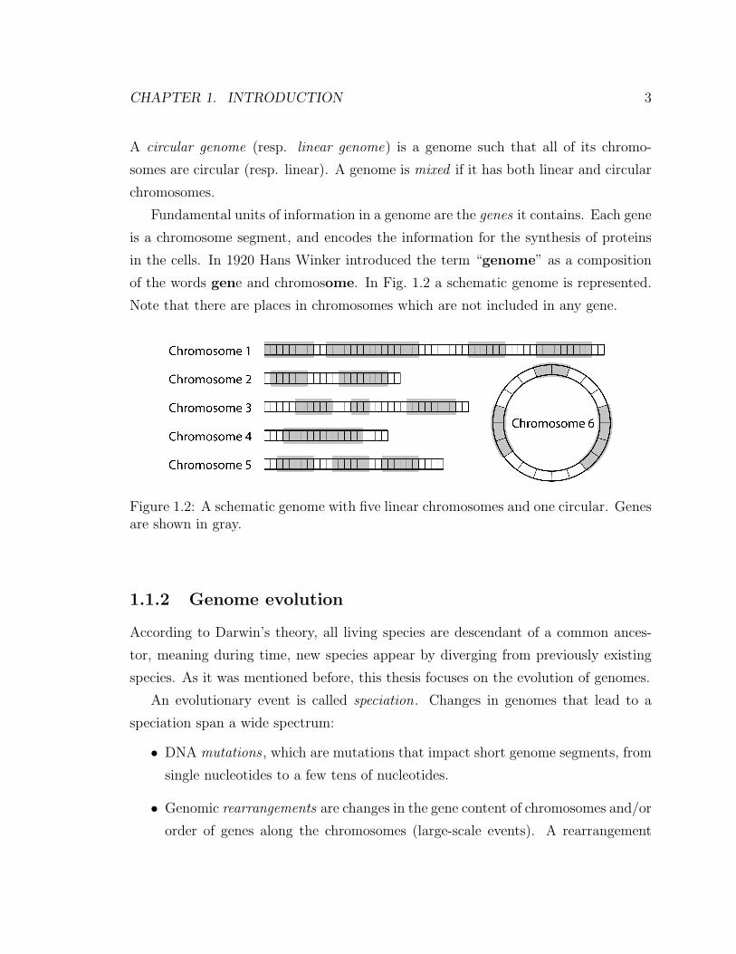
A circular genome (resp. linear genome) is a genome such that all of its chromo-
somes are circular (resp. linear). A genome is mixed if it has both linear and circular
chromosomes.
Fundamental units of information in a genome are the genes it contains. Each gene
is a chromosome segment, and encodes the information for the synthesis of proteins
in the cells. In 1920 Hans Winker introduced the term “genome” as a composition
of the words gene and chromosome. In Fig. 1.2 a schematic genome is represented.
Note that there are places in chromosomes which are not included in any gene.
Figure 1.2: A schematic genome with five linear chromosomes and one circular. Genesare shown in gray.
1.1.2 Genome evolution
According to Darwin’s theory, all living species are descendant of a common ances-
tor, meaning during time, new species appear by diverging from previously existing
species. As it was mentioned before, this thesis focuses on the evolution of genomes.
An evolutionary event is called speciation. Changes in genomes that lead to a
speciation span a wide spectrum:
• DNA mutations , which are mutations that impact short genome segments, from
single nucleotides to a few tens of nucleotides.
• Genomic rearrangements are changes in the gene content of chromosomes and/or
order of genes along the chromosomes (large-scale events). A rearrangement
CHAPTER 1. INTRODUCTION 4
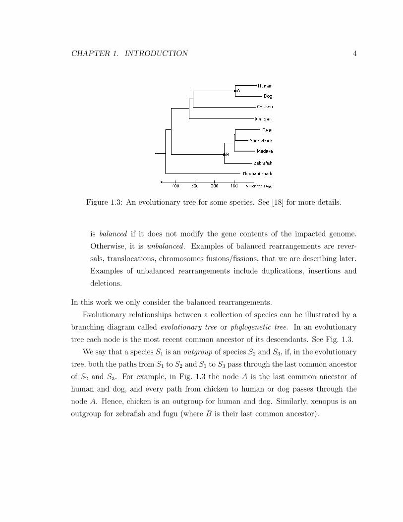
Figure 1.3: An evolutionary tree for some species. See [18] for more details.
is balanced if it does not modify the gene contents of the impacted genome.
Otherwise, it is unbalanced . Examples of balanced rearrangements are rever-
sals, translocations, chromosomes fusions/fissions, that we are describing later.
Examples of unbalanced rearrangements include duplications, insertions and
deletions.
In this work we only consider the balanced rearrangements.
Evolutionary relationships between a collection of species can be illustrated by a
branching diagram called evolutionary tree or phylogenetic tree. In an evolutionary
tree each node is the most recent common ancestor of its descendants. See Fig. 1.3.
We say that a species S1 is an outgroup of species S2 and S3, if, in the evolutionary
tree, both the paths from S1 to S2 and S1 to S3 pass through the last common ancestor
of S2 and S3. For example, in Fig. 1.3 the node A is the last common ancestor of
human and dog, and every path from chicken to human or dog passes through the
node A. Hence, chicken is an outgroup for human and dog. Similarly, xenopus is an
outgroup for zebrafish and fugu (where B is their last common ancestor).
CHAPTER 1. INTRODUCTION 5
1.2 Mathematical models
In this section we model genomes as discrete objects and rearrangements as discrete
operators on these objects. See [24] for graph theory terminology not explained here.
1.2.1 Modeling genomes
Suppose a chromosome, like in Fig. 1.4 (a), has 4 genes. In order to distinguish these
genes, we name them by distinct numbers 1, 2, 3, and 4. Also, we assign to each
gene a head (shown by h) and a tail (shown by t). Head and tail of a gene are called
extremities of that gene. The extremities of a genome is the set of all extremities of
its genes. Now the chromosome can be defined as the set of adjacencies between its
genes’ extremities. So, the chromosomes in Fig. 1.4 (a), (b), and (c) can be described
as:
• (a): {{1h, 2t}, {2h, 3t}, {3h, 4t}},
• (b): {{1h, 2h}, {2t, 3t}, {3h, 4t}},
• (c): {{1h, 2t}, {2h, 3t}, {3h, 4t}, {4h, 1t}}.
Figure 1.4: Genes’ extremities and their adjacencies. (a) and (b) two linear chromo-
somes having gene 2 in reverse directions, (c) a circular chromosome.
A gene extremity is a telomere if it is not adjacent to any other extremity, e.g., in
Fig. 1.4 (a) {1t} and {4h} are two telomeres. Note that the only difference between
CHAPTER 1. INTRODUCTION 6
chromosomes in Fig. 1.4 (a) and (b) is that the gene 2 appears in different (reverse)
direction along these chromosomes. To express this event, we mark this gene by 2
and −2, respectively. A genome can be represented as a set of adjacencies between its
extremities, by considering all of its chromosomes and their corresponding adjacencies.
1.2.2 Genome as a graph on extremities
Adjacencies of a genome can be represented by a graph called the breakpoint graph:
Definition Let G be a genome with gene set {1, 2, . . . , n}. The breakpoint graph of
the genome G, denoted by B(G), is a graph with {1h, 1t, . . . , nh, nt} as its vertex set
(extremities in G). Two vertices in B(G) are connected by an edge if they form an
adjacency in G.
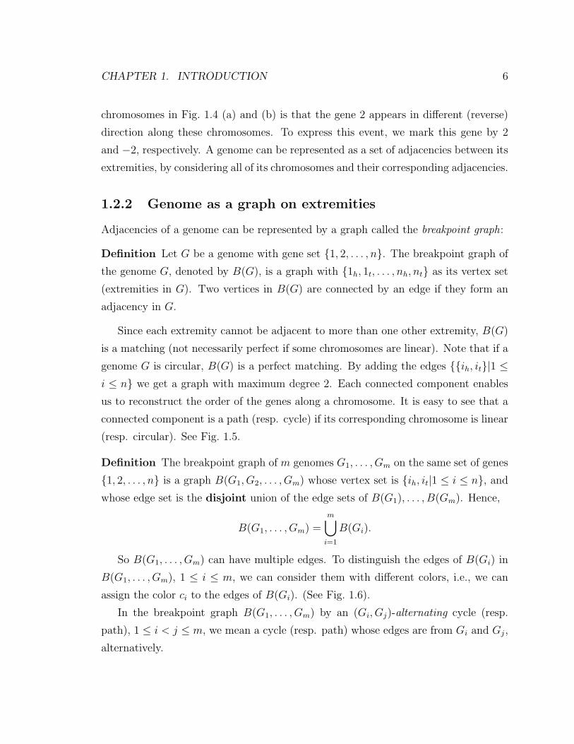
Since each extremity cannot be adjacent to more than one other extremity, B(G)
is a matching (not necessarily perfect if some chromosomes are linear). Note that if a
genome G is circular, B(G) is a perfect matching. By adding the edges {{ih, it}|1 ≤i ≤ n} we get a graph with maximum degree 2. Each connected component enables
us to reconstruct the order of the genes along a chromosome. It is easy to see that a
connected component is a path (resp. cycle) if its corresponding chromosome is linear
(resp. circular). See Fig. 1.5.
Definition The breakpoint graph of m genomes G1, . . . , Gm on the same set of genes
{1, 2, . . . , n} is a graph B(G1, G2, . . . , Gm) whose vertex set is {ih, it|1 ≤ i ≤ n}, and
whose edge set is the disjoint union of the edge sets of B(G1), . . . , B(Gm). Hence,
B(G1, . . . , Gm) =m⋃i=1
B(Gi).
So B(G1, . . . , Gm) can have multiple edges. To distinguish the edges of B(Gi) in
B(G1, . . . , Gm), 1 ≤ i ≤ m, we can consider them with different colors, i.e., we can
assign the color ci to the edges of B(Gi). (See Fig. 1.6).
In the breakpoint graph B(G1, . . . , Gm) by an (Gi, Gj)-alternating cycle (resp.
path), 1 ≤ i < j ≤ m, we mean a cycle (resp. path) whose edges are from Gi and Gj,
alternatively.
CHAPTER 1. INTRODUCTION 7
Figure 1.5: (a) A schematic genome with 10 genes, (b) its breakpoint graph, (c)connecting each gene’s extremities and reconstructing the chromosomes.
Figure 1.6: The breakpoint graph of three genomes with colors: black, bold black,and gray.
CHAPTER 1. INTRODUCTION 8
1.2.3 Modeling genome rearrangements
We consider here only rearrangements that preserve the gene content of a genome,
and we describe them as discrete operators.
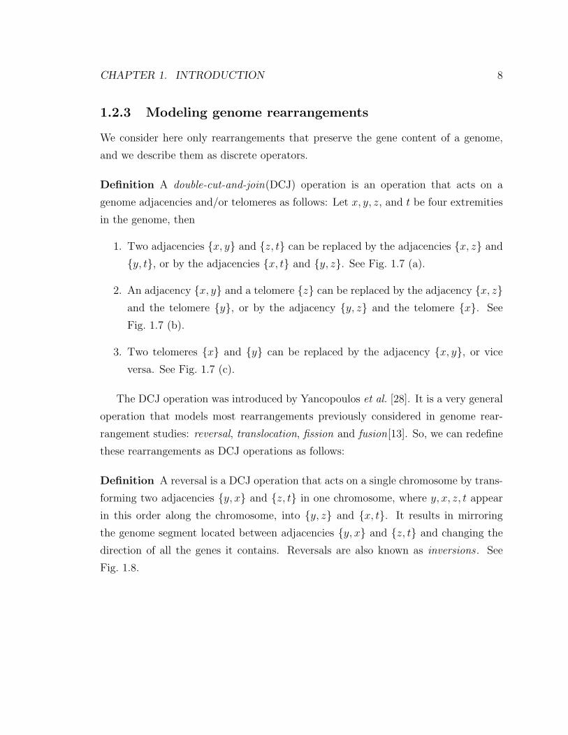
Definition A double-cut-and-join(DCJ) operation is an operation that acts on a
genome adjacencies and/or telomeres as follows: Let x, y, z, and t be four extremities
in the genome, then
1. Two adjacencies {x, y} and {z, t} can be replaced by the adjacencies {x, z} and
{y, t}, or by the adjacencies {x, t} and {y, z}. See Fig. 1.7 (a).
2. An adjacency {x, y} and a telomere {z} can be replaced by the adjacency {x, z}and the telomere {y}, or by the adjacency {y, z} and the telomere {x}. See
Fig. 1.7 (b).
3. Two telomeres {x} and {y} can be replaced by the adjacency {x, y}, or vice
versa. See Fig. 1.7 (c).
The DCJ operation was introduced by Yancopoulos et al. [28]. It is a very general
operation that models most rearrangements previously considered in genome rear-
rangement studies: reversal, translocation, fission and fusion[13]. So, we can redefine
these rearrangements as DCJ operations as follows:
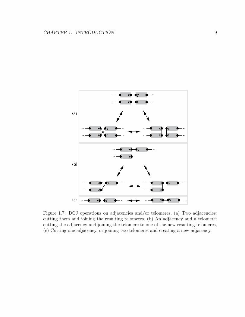
Definition A reversal is a DCJ operation that acts on a single chromosome by trans-
forming two adjacencies {y, x} and {z, t} in one chromosome, where y, x, z, t appear
in this order along the chromosome, into {y, z} and {x, t}. It results in mirroring
the genome segment located between adjacencies {y, x} and {z, t} and changing the
direction of all the genes it contains. Reversals are also known as inversions . See
Fig. 1.8.
CHAPTER 1. INTRODUCTION 9
Figure 1.7: DCJ operations on adjacencies and/or telomeres, (a) Two adjacencies:cutting them and joining the resulting telomeres, (b) An adjacency and a telomere:cutting the adjacency and joining the telomere to one of the new resulting telomeres,(c) Cutting one adjacency, or joining two telomeres and creating a new adjacency.
CHAPTER 1. INTRODUCTION 10
Figure 1.8: Reversal of a block. It is a DCJ operation acting on the adjacencies {x, y}and {z, t}.
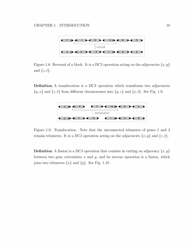
Definition A translocation is a DCJ operation which transforms two adjacencies
{y, x} and {z, t} from different chromosomes into {y, z} and {x, t}. See Fig. 1.9.
Figure 1.9: Translocation. Note that the unconnected telomeres of genes 1 and 3
remain telomeres. It is a DCJ operation acting on the adjacencies {x, y} and {z, t}.
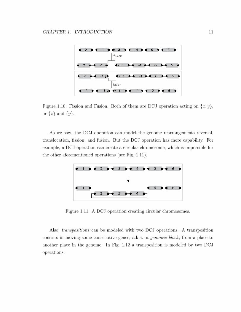
Definition A fission is a DCJ operation that consists in cutting an adjacency {x, y}between two gene extremities x and y, and its inverse operation is a fusion, which
joins two telomeres {x} and {y}. See Fig. 1.10 .
CHAPTER 1. INTRODUCTION 11
Figure 1.10: Fission and Fusion. Both of them are DCJ operation acting on {x, y},or {x} and {y}.
As we saw, the DCJ operation can model the genome rearrangements reversal,
translocation, fission, and fusion. But the DCJ operation has more capability. For
example, a DCJ operation can create a circular chromosome, which is impossible for
the other aforementioned operations (see Fig. 1.11).
Figure 1.11: A DCJ operation creating circular chromosomes.
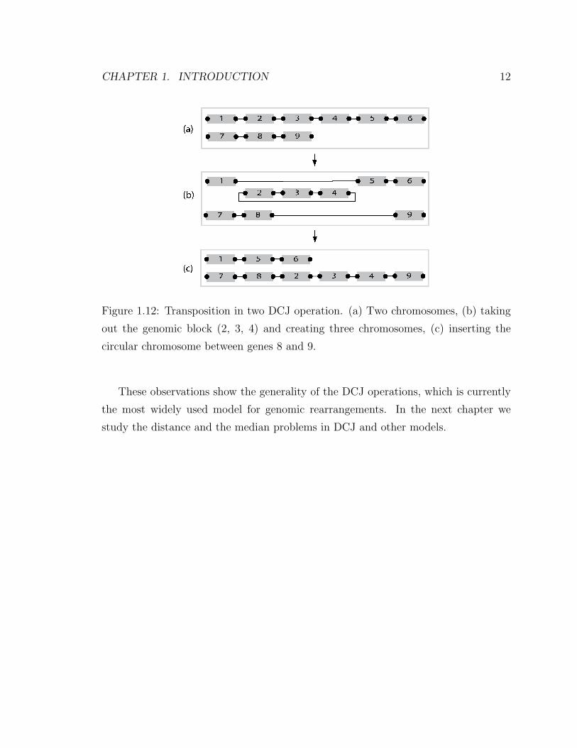
Also, transpositions can be modeled with two DCJ operations. A transposition
consists in moving some consecutive genes, a.k.a. a genomic block , from a place to
another place in the genome. In Fig. 1.12 a transposition is modeled by two DCJ
operations.
CHAPTER 1. INTRODUCTION 12
Figure 1.12: Transposition in two DCJ operation. (a) Two chromosomes, (b) taking
out the genomic block (2, 3, 4) and creating three chromosomes, (c) inserting the
circular chromosome between genes 8 and 9.
These observations show the generality of the DCJ operations, which is currently
the most widely used model for genomic rearrangements. In the next chapter we
study the distance and the median problems in DCJ and other models.
Chapter 2
Genomic Distance and Median
Problem
In this chapter, we introduce the notions of genomic distances, and median problems.
2.1 Distances
In Section 1.2.1 we stated that genomes can be modeled as discrete objects. A nat-
ural question is: How can we measure the similarity/dissimilarity of two genomes?
Genomic distances are good candidates for dissimilarity functions. Computing the
distances allows us to generate distance matrices between genomes, and infer parsi-
monious species trees (see Fig. 1.3). This problem was launched in a paper by David
Sankoff et al. [22].
Genomic distance can be the minimum number of allowed operations to transform
a genome to the other one, or only a function to show the dissimilarity between the
genomes. The former can be formalized as follows:
Given two genomes G1 and G2 on the same set of genes, a set of allowed
rearrangements R, and an optimality criterion C. An evolutionary sce-
nario S = s1, s2, . . . , sk is a sequence of rearrangements si ∈ R, and C is a
function from all possible scenarios to real numbers. What is an optimal
13
CHAPTER 2. GENOMIC DISTANCE AND MEDIAN PROBLEM 14
scenario S, i.e., it minimizes C(S)?
The answer to this question depends on our choice for the model (R, C). It can
be tractable or intractable by assuming different models. Parsimony is a widely used
criterion in which we try to minimize the number of rearrangements, i.e., among all
evolutionary scenarios S = s1, s2, . . . , sk we want to minimize k. In this work, we
always assume parsimony as the optimality criterion.
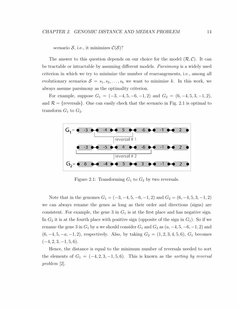
For example, suppose G1 = (−3,−4, 5,−6,−1, 2) and G2 = (6,−4, 5, 3,−1, 2),
and R = {reversals}. One can easily check that the scenario in Fig. 2.1 is optimal to
transform G1 to G2.
Figure 2.1: Transforming G1 to G2 by two reversals.
Note that in the genomes G1 = (−3,−4, 5,−6,−1, 2) and G2 = (6,−4, 5, 3,−1, 2)
we can always rename the genes as long as their order and directions (signs) are
consistent. For example, the gene 3 in G1 is at the first place and has negative sign.
In G2 it is at the fourth place with positive sign (opposite of the sign in G1). So if we
rename the gene 3 in G1 by a we should consider G1 and G2 as (a,−4, 5,−6,−1, 2) and
As mentioned in the previous chapter, we only consider the DCJ median problem of
mixed multi-chromsomal genomes and a circular median. So a circular DCJ median
for three genomes G1, G2, and G3 on the same set of n genes, is a circular genome M
which minimizes
3∑i=1
dDCJ(Gi,M) = 3n− c(G1,M)− c(G2,M)− c(G3,M),
(see Section 2.1.2) and it is equivalent to
maximize3∑i=1
c(Gi,M). (3.1)
Therefore, a genome M that maximizes the total number of (M,Gi)-alternating cycles
(for i ∈ {1, 2, 3} ) is a circular DCJ median. In this work, we consider the maximiza-
tion case. An alternating cycle is a (M,Gi)-alternating cycle for some i, 1 ≤ i ≤ 3.
For the sake of simplicity, by median we always mean the circular DCJ median.
We can generalize the concept of breakpoint graph to any 3-edge-colored graph,
and define the median problem as follows:
Definition A breakpoint graph B(G1, G2, G3) is a 3-edge-colored graph with color
25
CHAPTER 3. TRACTABLE INSTANCES FOR THE DCJ MEDIAN PROBLEM26
classes G1, G2, and G3. A median of B is a matching M on vertices of B, which
maximizes3∑i=1
c(Gi,M).
3.1 Preliminaries
Let B = B(G1, G2, G3) be the breakpoint graph, and let M be a median of B. The
graph BM(G1, G2, G3) = B ∪M is called the median graph of B with the median
genome M . Also, by cyc(B) we mean the number of alternating cycles in the median
graph BM .
Remark The edges of a breakpoint graph are colored, and cyc is a function from
3-edge-colored graphs to integer numbers. Hence, cyc(B) does not depend only on
the topology of B, but also on the colors of its edges.
Remark Note that for different medians M of B, BM has the same number of alter-
nating cycles.
From now on, for a given median graph BM(G1, G2, G3), edges in G1 ∪ G2 ∪ G3
are called colored edges, and edges in M are called median edges. When the context
is clear, we only use BM for BM(G1, G2, G3). By a k-cycle in a 3-edge-colored graph,
we mean an alternating cycle with k vertices.
Let H be a subgraph of the breakpoint graph B. An H-crossing edge in the
median graph BM is a median edge which connects a vertex in V (H) to a vertex in
V (B)− V (H). By an H-crossing cycle we mean an alternating cycle which contains
at least one H-crossing edge. The subgraph H is k-independent if there is a median
M for B such that the number of H-crossing edges in BM is at most k. We denote
by Ck (resp. Pk) a subgraph of B that is isomorphic to a cycle (resp. path) with k
vertices.
The following operation was defined in [27]: shrinking a pair of vertices {u, v} or
an edge with vertices u and v consists of: (1) removing all edges between u and v,
(2) identifying the edges with same color incident to u and v, (3) removing u and v.
We denote the resulting graph by B · {u, v} (Fig. 3.1).
CHAPTER 3. TRACTABLE INSTANCES FOR THE DCJ MEDIAN PROBLEM27
Figure 3.1: Shrinking a pair {u, v}
Proposition 3.1.1 Let B be the breakpoint graph of genomes G1, . . . , Gm, and u, v ∈V (B). Suppose that there are k colored edges between u and v. If there exists a median
containing uv, then cyc(B) = cyc(B · {u, v}) + k.
Proof Consider a median M which contains the edge uv. Let B′ = B · {u, v},M ′ = M −{u, v}, and C be an alternating cycle in BM . If C does not contain {u, v},then it is easy to see that since {u, v} is in M , C does not contain any of the k edges
between u and v. Thus, C remains in B′ ∪M ′, without change. So assume that C
contains uv. If its length is larger than 2, shrinking {u, v} results in a cycle with
smaller length in B′∪M ′ (2 units smaller). Otherwise, if it has length 2, it disappears
in B′ ∪M ′. Thus the number of alternating cycles which disappear in B′ ∪M ′ is k,
since there are k edges between u and v. Therefore, cyc(B) ≤ cyc(B · {u, v}) + k.
Now suppose N is a median for B′. By a similar argument, if N ′ = N ∪ {u, v},then B∪N ′ has cyc(B ·{u, v})+k alternating cycles. So, cyc(B) ≥ cyc(B ·{u, v})+k,
and we have cyc(B) = cyc(B ·{u, v})+k, which means that M ′ (resp. N ′) is a median
for B′ (resp. B).
3.2 A class of tractable instances
Our main result covers a large class of tractable instances for the median problem.
Obviously, the median problem for three genomes involves a breakpoint graph with
maximum degree 3. We hint here that the hardness of the problem is due to the
CHAPTER 3. TRACTABLE INSTANCES FOR THE DCJ MEDIAN PROBLEM28
vertices of degree 3.
Theorem 3.2.1 Let G1, G2, and G3 be three genomes. If there exists a median of
B(G1, G2, G3) with at most ` edges whose both end-vertices are of degree 3, then
computing such a median can be done in time O(n3 · (`+ 1) · (3m ·m2` + 1)), where m
is the number of vertices of degree 3, and n is the number of genes in B(G1, G2, G3).
Note that, as corollaries of this theorem, we have:
1. if m is bounded, then computing a median is tractable,
2. if ` is bounded, then computing a median is FPT with parameter m,
3. if m is not bounded, we can remove some edges incident to vertices of degree 3,
so that in the new instance m′ (the number of vertices of degree 3 in the newer
graph) is bounded. Now, by the case 1, there is a polynomial time algorithm
which computes the median of the new instance. We approximate the median
of the original problem by this median.
Informally, to prove Theorem 3.2.1, we first consider all possibilities (configura-
tions) for matching vertices of degree 3. For each configuration, we reduce the break-
point graph by shrinking and removing some edges to obtain a graph with maximum
degree 2 whose connected components will be paths or cycles. Next, we compute a
median of the remaining breakpoint graph in polynomial time. This will follow since
we show that there exists at least one median M such that: (1) every even component
of B(G1, G2, G3) has no crossing edge, so they can be considered independently and
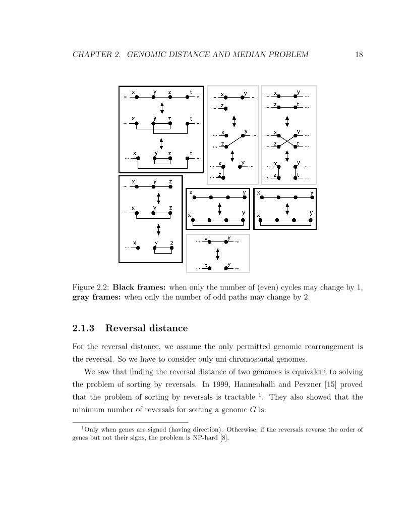
(2) odd components B(G1, G2, G3) are matched with each other. See Fig 3.2.
CHAPTER 3. TRACTABLE INSTANCES FOR THE DCJ MEDIAN PROBLEM29
Figure 3.2: (e) Each even component has no crossing edge, (o) For each odd com-
ponent H1, there is exactly another odd component H2, such that (H1 ∪H2) has no
crossing edge.
From now, G1, G2, and G3 are mixed multi-chromosomal genomes on n genes, and
M is a circular median of these genomes, unless otherwise specified. We denote their
breakpoint graph by B, and the median graph by BM .
3.2.1 Independence of even cycles and paths
In this section we show that if a connected component of B is isomorphic to an even
cycle or even path, it is 0-independent (i.e. each can be processed independently
from the other connected components) and if it is isomorphic to an odd path it is
1-independent. We first state two auxiliary results.
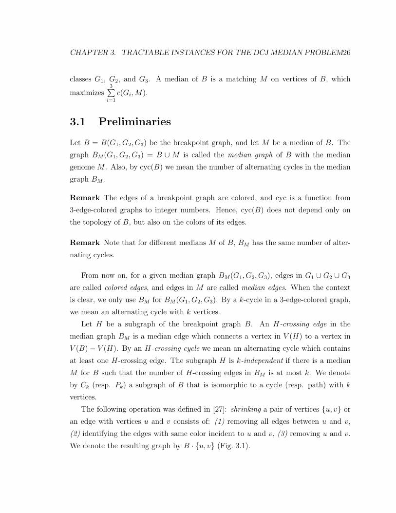
Lemma 3.2.2 If B is isomorphic to Pk or C2k, for k ≥ 1, then for every subgraph
H ⊆ B, cyc(H) ≥ |E(H)|2
.
Proof Consider the path Pk = u1u2 . . . uk. Let M be the matching consisting of the
edges u1u2, u3u4, . . ., and ut−1ut, where t = 2bk2c. Obviously, the number of alternating
cycles in Pk ∪M is bk/2c, so cyc(Pk) ≥ k2≥ |E(Pk)|
2. Similarly cyc(C2k) ≥ k = |E(C2k)|
2.
see Fig. 3.3.
Any proper subgraph H ⊂ Pk or C2k is a union of disjoint paths. If we take the
union of matchings described above for each of these paths and call it M , there are
at least |E(H)|/2 alternating cycles in H ∪M . Therefore for any subgraph H ⊆ B,
cyc(H) ≥ |E(H)|2
.
CHAPTER 3. TRACTABLE INSTANCES FOR THE DCJ MEDIAN PROBLEM30
Figure 3.3: Median edges (dashed) for cycles and union of disjoint paths.
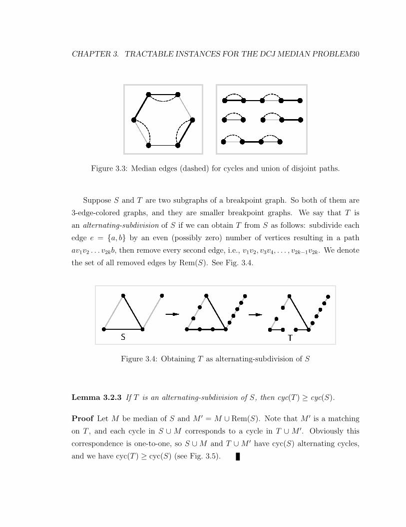
Suppose S and T are two subgraphs of a breakpoint graph. So both of them are
3-edge-colored graphs, and they are smaller breakpoint graphs. We say that T is
an alternating-subdivision of S if we can obtain T from S as follows: subdivide each
edge e = {a, b} by an even (possibly zero) number of vertices resulting in a path
av1v2 . . . v2kb, then remove every second edge, i.e., v1v2, v3v4, . . . , v2k−1v2k. We denote
the set of all removed edges by Rem(S). See Fig. 3.4.
Figure 3.4: Obtaining T as alternating-subdivision of S
Lemma 3.2.3 If T is an alternating-subdivision of S, then cyc(T ) ≥ cyc(S).
Proof Let M be median of S and M ′ = M ∪ Rem(S). Note that M ′ is a matching
on T , and each cycle in S ∪ M corresponds to a cycle in T ∪ M ′. Obviously this
correspondence is one-to-one, so S ∪M and T ∪M ′ have cyc(S) alternating cycles,
and we have cyc(T ) ≥ cyc(S) (see Fig. 3.5).
CHAPTER 3. TRACTABLE INSTANCES FOR THE DCJ MEDIAN PROBLEM31
Figure 3.5: Obtaining a matching for T from the median of S (dashed edges are themedian edges)
Proposition 3.2.4 Let H be a connected component of B. If H is isomorphic to P2k
or C2k, for k ≥ 1, then H is 0-independent.
Proof Let M be a median of B. Suppose M has ` H-crossing edges in BM . If ` = 0,
then we are done, so assume that ` > 0. Since H has an even number of vertices, `
is even and ` ≥ 2. Because H is a connected component in B, each H-crossing cycle
contains an even number of H-crossing edges.
Let C(M) be the set of all H-crossing cycles in the median graph BM , and Cr(M)
be the set of all H-crossing edges. Let X(M) be the set of colored edges in all cycles
of C(M), and Y(M) be the set of all H-crossing edges in all cycles of C(M).
If there is no H-crossing cycle, i.e., C(M) = Y(M) = ∅, we modify M by removing
all H-crossing edges, and re-matching the vertices inside of H together and outside
of H together. Since ` is even, this is always possible and we get a median with no
H-crossing edge. So assume that there exists at least one H-crossing cycle.
We introduce a transformation on M such that after each step we obtain another
median of B with fewer H-crossing edges (decreasing |Cr(M)|) or the same number
of H-crossing edges but with fewer edges in H-crossing cycles (implies the decrement
in |X(M)|). After this transformation, we obtain a median with no H-crossing cycle.
Each step of the transformation is as follows: from each H-crossing cycle we pick one
colored edge in H incident to an H-crossing edge in that cycle arbitrarily. Let S be the
subgraph of B induced by these picked colored edges. Since every colored edge is in
at most one alternating cycle and since two edges of the same color are independent,
CHAPTER 3. TRACTABLE INSTANCES FOR THE DCJ MEDIAN PROBLEM32
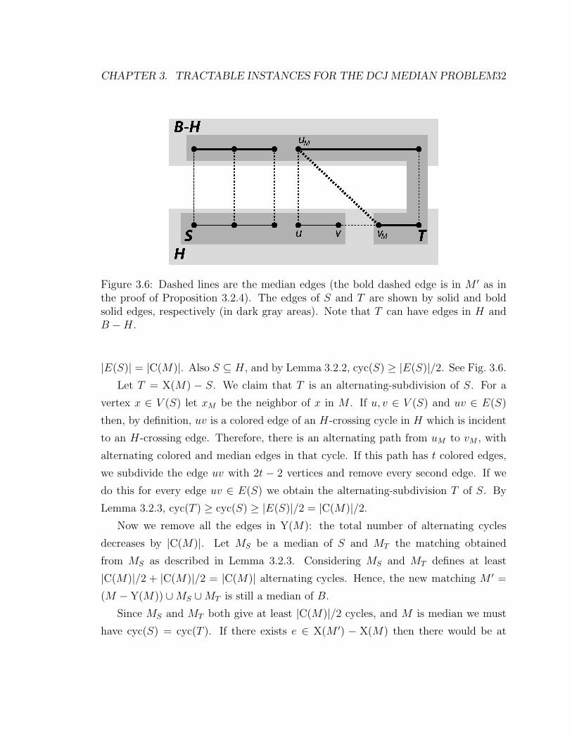
Figure 3.6: Dashed lines are the median edges (the bold dashed edge is in M ′ as inthe proof of Proposition 3.2.4). The edges of S and T are shown by solid and boldsolid edges, respectively (in dark gray areas). Note that T can have edges in H andB −H.
|E(S)| = |C(M)|. Also S ⊆ H, and by Lemma 3.2.2, cyc(S) ≥ |E(S)|/2. See Fig. 3.6.
Let T = X(M) − S. We claim that T is an alternating-subdivision of S. For a
vertex x ∈ V (S) let xM be the neighbor of x in M . If u, v ∈ V (S) and uv ∈ E(S)
then, by definition, uv is a colored edge of an H-crossing cycle in H which is incident
to an H-crossing edge. Therefore, there is an alternating path from uM to vM , with
alternating colored and median edges in that cycle. If this path has t colored edges,
we subdivide the edge uv with 2t − 2 vertices and remove every second edge. If we
do this for every edge uv ∈ E(S) we obtain the alternating-subdivision T of S. By
Now we remove all the edges in Y(M): the total number of alternating cycles
decreases by |C(M)|. Let MS be a median of S and MT the matching obtained
from MS as described in Lemma 3.2.3. Considering MS and MT defines at least
|C(M)|/2 + |C(M)|/2 = |C(M)| alternating cycles. Hence, the new matching M ′ =
(M − Y(M)) ∪MS ∪MT is still a median of B.
Since MS and MT both give at least |C(M)|/2 cycles, and M is median we must
have cyc(S) = cyc(T ). If there exists e ∈ X(M ′) − X(M) then there would be at
CHAPTER 3. TRACTABLE INSTANCES FOR THE DCJ MEDIAN PROBLEM33
least one H-crossing cycle induced by M ′ which is not induced by MS or MT , so the
number of alternating cycles in BM ′ would be more than the number of alternating
cycles in BM , which is a contradiction, because BM and BM ′ have the same number
of alternating cycles. Regarding the fact that S 6= ∅, we have X(M ′) ⊂ X(M), since
E(S) ⊂ X(M) and E(S) ∩X(M ′) = ∅ (the vertices in S are matched to themselves).
We now show that |Cr(M ′)| ≤ |Cr(M)|. An edge e in M ′ is H-crossing edge only
if e = uMvM ∈ MT , where u, v ∈ V (S), vM ∈ H, uM ∈ B − H, and uv ∈ MS (see
Lemma 3.2.3, how we get MT from MS). This implies that uuM is an H-crossing edge
in M . Now by assigning uuM to uMvM we obtain a one-to-one function from Cr(M ′)
to Cr(M), since uuM and uMvM are incident and M ′ is a matching and different edges
in Cr(M ′) are assigned to different edges in Cr(M). Hence |Cr(M ′)| ≤ |Cr(M)|. We
have |X(M ′)|+ |Cr(M ′)| < |X(M)|+ |Cr(M)|, and by iterating all steps above we get
a median without any H-crossing edge.
Remark The transformation introduced in the proof of Proposition 3.2.4 can be
applied as long as there are at least two H-crossing edges. Because when there is
no H-crossing cycle and there are at least two H-crossing edges, we can remove two
of them and match their end-vertices in H together and other end-vertices together.
Otherwise, if there is at least one H-crossing cycle we can define S and T as before
and continue our transformation steps.
Lemma 3.2.5 Let H be a connected component of B. If H is isomorphic to P2k−1,
for k ≥ 1, then H is 1-independent. Moreover, there exists a median in which the
H-crossing edge is incident to one of the terminal vertices (vertices of degree one) of
H.
Proof From Lemma 3.2.2, we know that for every subgraph H ′ ⊆ P2k−1 we have
cyc(H ′) ≥ |E(H ′)|/2. Now by using the transformation introduced in the proof of
Proposition 3.2.4 and by previous remark, we can obtain a median with exactly 1
H-crossing edge. Note that if there is only one H-crossing edge it cannot be in
any H-crossing cycle, and by Proposition 3.2.7 below (which shows that cyc(Pn) is
independent from edge colors in Pn) we can connect that crossing edge to a terminal
vertex of H.
CHAPTER 3. TRACTABLE INSTANCES FOR THE DCJ MEDIAN PROBLEM34
Lemma 3.2.6 For the breakpoint graph B there exists a median in which even com-
ponents have no crossing edge, and each odd path has exactly one crossing edge.
Proof It is easy to see that for each even/odd path or even cycle we can do the
transformation in Proposition 3.2.4 on a current median and reduce the crossing
edges for each of them, without increasing the number of crossing edges in other
components.
3.2.2 Computing cyc for paths and even cycles
The results of the previous section open the way to computing a median of a break-
point graph with maximum degree 2 by considering each path or even cycle inde-
pendently (for odd paths we consider only one crossing edge connected to one of its
terminal vertices). Here, first we show that computing a median of an even con-
nected component or an odd path is tractable. In the following let H be a connected
component of B.
Proposition 3.2.7 If H is isomorphic to Pk, for k ≥ 1, then cyc(H) = bk2c.
Proof From Lemma 3.2.2 cyc(H) ≥ bk2c. To prove the equality we use induction on
k. It obviously holds for k = 1. So we assume that k ≥ 2, and consider a median
M for H. If there is no 2-cycle (i.e., E(H) ∩M = ∅; a 2-cycle is a cycle with length
two which is consist of two parallel edges, denoted by C2), each alternating cycle
has length ≥ 4; since in each alternating cycle there are at least 2 colored edges,
cyc(H) ≤ b |E(H)|2c = bk−1
2c ≤ bk
2c.
Now assume that the median M contains a 2-cycle. So there is an edge uv ∈E(H) ∩ M . Shrinking {u, v} results in H ′ that is either a single path with k − 2
vertices or two paths with p and q vertices such that p + q = k − 2. In both cases,
using induction and the fact that all paths are 0-independent or 1-independent, we
obtain that in the case:
• of one remaining path cyc(H ′) ≤ bk−22c+ 1 = bk
2c.
• of two remaining paths cyc(H ′) ≤ bp2c+ b q
2c+ 1 ≤ bk
2c.
CHAPTER 3. TRACTABLE INSTANCES FOR THE DCJ MEDIAN PROBLEM35
This completes the proof and it is easy to see that the time needed to find a median
of Pk is O(k).
Remark Note that if H is isomorphic to Pk, then cyc(H) is independent from the
edge coloring of H.
Lemma 3.2.8 If H is isomorphic to C2k, for k ≥ 1, then either cyc(H) = k or k+1.
Proof Taking the edges of H, alternatively as a matching M , results in a graph with
k 2-cycles, so cyc(H) ≥ k. Note that when k = 4, cyc(C4) = 3 = 42
+ 1. Also
cyc(C2) = 2 = 22
+ 1.
Now assume that cyc(H) > k. We claim that there is at least one 2-cycle in any
median graph. As in Proposition 3.2.7, if all alternating cycles in the median graph
HM have length at least 4, then the number of alternating cycles is at most k, so
there must exist at least one 2-cycle. Let {u, v} be the colored edge in that 2-cycle:
cyc(H) = cyc(H · {u, v}) + 1 (Proposition 3.1.1). Obviously, H · {u, v} is a path,
or a cycle, and it is a cycle if and only if the two edges incident to {u, v} have the
same color. If it is a path, Proposition 3.2.7 implies that cyc(H · {u, v}) = k − 1
and cyc(H) = k, which contradicts the assumption that cyc(H) > k. So H · {u, v}is a cycle and the edges incident to uv have same color. By induction we can find
a median of H · {u, v} with cyc(H · {u, v}) = k − 1 + 1 or cyc(H · {u, v}) = k − 1,
alternating cycles. Hence, cyc(H) = k + 1 or cyc(H) = k.
Remark By previous theorem, if H is isomorphic to C2k, then cyc(H) dependents
on the edge coloring of H.
We say that a cycle C2k is of the first kind if cyc(C2k) = k, and it is of the second
kind if cyc(C2k) = k + 1 (see Fig. 3.7). We show below how to decide in polynomial
time if an even cycle is of the first or second kind.
In a cycle C, the signature of a vertex is an ordered pair (a, b) such that a and
b are the colors of the edges incident to that vertex. We define signature of vertices
of a cycle with respect to a fixed orientation of the cycle; a will be the color of the
incoming edge and b the color of the outgoing edge.
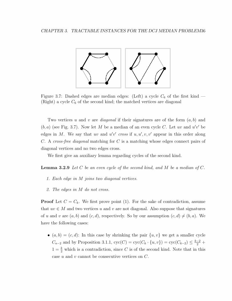
CHAPTER 3. TRACTABLE INSTANCES FOR THE DCJ MEDIAN PROBLEM36
Figure 3.7: Dashed edges are median edges: (Left) a cycle C6 of the first kind —(Right) a cycle C6 of the second kind; the matched vertices are diagonal
Two vertices u and v are diagonal if their signatures are of the form (a, b) and
(b, a) (see Fig. 3.7). Now let M be a median of an even cycle C. Let uv and u′v′ be
edges in M . We say that uv and u′v′ cross if u, u′, v, v′ appear in this order along
C. A cross-free diagonal matching for C is a matching whose edges connect pairs of
diagonal vertices and no two edges cross.
We first give an auxiliary lemma regarding cycles of the second kind.
Lemma 3.2.9 Let C be an even cycle of the second kind, and M be a median of C.
1. Each edge in M joins two diagonal vertices.
2. The edges in M do not cross.
Proof Let C = Ck. We first prove point (1). For the sake of contradiction, assume
that uv ∈M and two vertices u and v are not diagonal. Also suppose that signatures
of u and v are (a, b) and (c, d), respectively. So by our assumption (c, d) 6= (b, a). We
have the following cases:
• (a, b) = (c, d): In this case by shrinking the pair {u, v} we get a smaller cycle
Cn−2 and by Proposition 3.1.1, cyc(C) = cyc(Ck · {u, v}) = cyc(Ck−2) ≤ k−22
+
1 = k2
which is a contradiction, since C is of the second kind. Note that in this
case u and v cannot be consecutive vertices on C.
CHAPTER 3. TRACTABLE INSTANCES FOR THE DCJ MEDIAN PROBLEM37
• (a, b) 6= (c, d): Now by shrinking the pair {u, v}, the remaining graph can be
one of the following:
– A path with k − 2 vertices,
– A cycle and a path, together with k − 2 vertices.
In the first case, vertices u and v must be consecutive on C. But now cyc(C) =
cyc(Ck · {u, v}) + 1 = cyc(Pk−2) + 1 = k−22
+ 1 < k2
+ 1, which is a contradiction,
since C is of the second kind. In the second case cyc(C) = cyc(Ck · {u, v}) =
cyc(C`) + cyc(Pm) ≤ `2
+ 1 + m2≤ k−2
2+ 1 < k
2+ 1, since paths are either 0- or
1-independent and ` + m = k − 2 (note that in the latter case u and v cannot
be consecutive). This is again a contradiction since C is of second kind.
We now prove point (2). Since the cycle C is of the second kind, it follows from
the proof of Lemma 3.2.8, there is a 2-cycle with colored edge {u′, v′} (which is also
an edge in M), and by point (1), vertices u′ and v′ are diagonal. So Ck · {u′, v′} is the
Ck−2 cycle and it must be of the second kind, as otherwise cyc(Ck) = cyc(Ck−2)+1 =k−22
+ 1 = k2< k
2+ 1. Obviously, {u′, v′} does not cross with any median edges of M .
By shrinking this pair and using the induction on Ck · {u′, v′} the proof is complete.
Lemma 3.2.10 An even cycle C is of the second kind if and only if there exists a
matching M of C that is cross-free diagonal.
Proof Assume C = Ck. The necessity follows from Lemma 3.2.9. Now, assume
that there exists a cross-free diagonal matching M on vertices of C. It is easy to
see that M contains edge {u, v} where u and v are consecutive on C (note that M
is a perfect matching, since we only consider circular medians). If we shrink the
pair {u, v}, the resulting graph is Ck−2 and remaining edges of M are a cross-free
diagonal matching for Ck−2. We can complete the proof by induction on k, since
cyc(Ck) = 1 + cyc(Ck−2) = 1 + k−22
+ 1 = k2
+ 1, and the statement of the lemma is
obviously true for k = 2.
CHAPTER 3. TRACTABLE INSTANCES FOR THE DCJ MEDIAN PROBLEM38
Lemma 3.2.11 Let C be an even cycle. Deciding if C admits a cross-free diagonal
matching is tractable.
Proof Let Ck = v1v2 . . . vk, and k be even. We use the following greedy algorithm to
compute a median M (in fact a classical algorithm for deciding if a parenthesis word
is balanced):
1. M = ∅ (v1, v2, . . . , vk are not matched)
2. For j = 1 to k
(a) if there exists i (1 ≤ i < j), such that vi and vj are diagonal, vi is not
matched, and i is the maximum number with this property, then add
{vi, vj} to M (match vi and vj).
3. If all vertices are matched, C has a cross-free diagonal matching, otherwise it
does not.
The time complexity of this algorithm is O(k2): we iterate the loop k times and
for each j in the loop we check previous vertices to find the proper i. One can easily
see that this can be done in linear time as follows:
1. S = ∅ is a stack.
2. For j = 1 to k
(a) if the top element of S is diagonal with vj, pop it from the stack S.
(b) else, push vj on S.
3. If S is empty, C has a cross-free diagonal matching, otherwise it does not.
Proposition 3.2.12 Let C be an even cycle of size k (k ≥ 2). Computing cyc(C)
can be done in time O(k).
Proof Immediate consequence of Lemma 3.2.8, Lemma 3.2.10, and Lemma 3.2.11.
CHAPTER 3. TRACTABLE INSTANCES FOR THE DCJ MEDIAN PROBLEM39
3.3 Proof of Theorem 3.2.1
We first prove that finding a median of a breakpoint graph of maximum degree two
with only odd components can be done in polynomial time. We need the following
lemma.
Lemma 3.3.1 If B has maximum degree 2 and consists of two odd connected com-
ponents, then computing a median of B is tractable.
Proof Let H1 and H2 be the two odd connected components of B. Obviously, a
median M contains an edge e between H1 and H2 (e is a H1-crossing edge). If one
of H1 and H2 is a path, then, by Lemma 3.2.5, we can assume e is connected to its
terminal vertex. In either case, by shrinking e we get an even connected component
or two even connected components, whose medians can be computed independently
in polynomial time. There are at most |V (H1)| × |V (H2)| possible candidates for e,
and for each candidate in time O(|V (H1)|+ |V (H2)|) we calculate the median. Hence
computing a median of B is tractable in time O(|V (H1)|·|V (H2)|·(|V (H1)|+|V (H2)|)).
Lemma 3.3.2 If B has maximum degree 2, then there exists a median of B such
that every odd connected component of B is connected by median edges to exactly one
other odd connected component.
Proof Let M be the median described in Lemma 3.2.6, and from Lemma 3.2.5 we can
assume that for each odd path there exists exactly one crossing edge of M connected
to its terminal vertex. Now consider an odd component H and one of its crossing
edges, say e, that connects H to another odd component H ′. By shrinking e we get
(H ∪H ′) · e which is a set of even components and it is then independent.
So M can be modified into a median without any edge leaving H∪H ′. This means
that H and H ′ are linked together and nothing else. Using this argument for other
odd components and the fact that the number of odd components is even (because
the number of vertices in the breakpoint graph is even), we arrive to a median that
satisfies the lemma (see Fig 3.2).
CHAPTER 3. TRACTABLE INSTANCES FOR THE DCJ MEDIAN PROBLEM40
Proposition 3.3.3 If B is a breakpoint graph with 2n vertices and consisting of only
odd cycle(s)/path(s), then computing a median of B can be done in O(n3).
Proof We first define a complete edge-weighted graph KB as follows:
1. each connected component C defines a vertex vC ;
2. each edge {vC , vD} has weight cyc(C ∪D)
By Lemma 3.3.1, KB is computable in polynomial time. We claim it is computable
in O(n3). Suppose B has t components and n1, . . . , nt are the number of vertices in
each component. So we have n1 + . . .+nt = 2n. The time to construct KB is of order
∑i<j
ni · nj · (ni + nj) =∑i<j
n2i · nj + ni · n2
j =1
3((2n)3 − (n3
1 + . . .+ n3t )) ≤
8
3n3.
Finally, by Lemma 3.3.2 we only need to find a maximum weight matching for KB,
which can be done in O(n3) by using Edmonds’s algorithm [12] (one can consider any
algorithm for finding the maximum matching without changing the total complexity,
as long as it is in O(n3), since constructing KB is in O(n3)).
If the breakpoint graph B has maximum degree 2, its connected components are
paths and cycles. By Lemma 3.2.6 and Proposition 3.2.12 we can find the median
edges for even components independently. Finally for odd components we find the
median edge by Proposition 3.3.3.
Handling vertices of degree 3. We now assume that B(G1, G2, G3) has maximum
degree 3. We consider all possibilities for matching the vertices of degree 3. A vertex
u of degree 3 can be matched in two ways:
• to another vertex of degree 3. By shrinking these two vertices, obtain a smaller
graph with fewer vertices of degree 3;
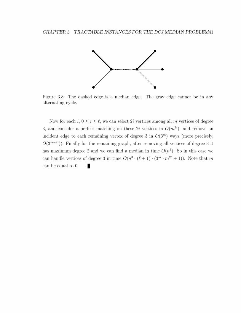
• to another vertex of degree less than 3. This implies that one of the edges
incident to u is not in any alternating cycle, and we can remove this edge and
transform u into a vertex of degree 2 (Fig. 3.8).
CHAPTER 3. TRACTABLE INSTANCES FOR THE DCJ MEDIAN PROBLEM41
Figure 3.8: The dashed edge is a median edge. The gray edge cannot be in anyalternating cycle.
Now for each i, 0 ≤ i ≤ `, we can select 2i vertices among all m vertices of degree
3, and consider a perfect matching on these 2i vertices in O(m2i), and remove an
incident edge to each remaining vertex of degree 3 in O(3m) ways (more precisely,
O(3m−2i)). Finally for the remaining graph, after removing all vertices of degree 3 it
has maximum degree 2 and we can find a median in time O(n3). So in this case we
can handle vertices of degree 3 in time O(n3 · (` + 1) · (3m ·m2` + 1)). Note that m
can be equal to 0.
Chapter 4
Conclusion
In this work, we specified a large class of tractable instances for the DCJ median
problem (with circular median and mixed genomes). In fact, we proved that only the
vertices of degree 3 make the problem intractable. Also, by removing k edges from
the breakpoint graph and decreasing its maximum degree, score of its median is not
smaller than k units less than the score of the main median (i.e. the current score +
k is an upper bound for the score of the main median). Finally, we showed there is
an FPT algorithm for the DCJ median problem, if there always exists a median such
that the number of its edges connecting two vertices of degree 3 is bounded.
From a theoretical point of view, it raises several interesting questions. First, it
leaves open the possibility that the DCJ median problem is FPT. The next obvious
problem is to extend our approach to the case of a mixed or linear median. This
would require to understand better the combinatorics of odd paths in the breakpoint
graphs.
Another interesting question is about expanding the breakpoint distance toward
the DCJ distance: As we saw in Chapter 2, for two genomes G1 and G2 on n genes,
their breakpoint distance is equal to
dBP(G1, G2) = n− a(G1, G2)−1
2e(G1, G2).
The parameters a(G2, G2) and e(G1, G2) are also equal the number of 2-cycles and
1-paths (P1) in the breakpoint graph B(G1, G2), respectively. The DCJ distance of
42
CHAPTER 4. CONCLUSION 43
these genomes is:
dDCJ(G1, G2) = n− c(G1, G2)−p(G1, G2)
2,
where c(G1, G2) and p(G1, G2) are the number of (even) cycles and odd paths in the
B(G1, G2), respectively. This motivates us to define a dissimilarity function as follows:
d(i,j)(G1, G2) = n− ci(G1, G2)−1
2pj(G1, G2),
where ci(G1, G2) is the number of (even) cycles with at most 2i vertices, and pj(G1, G2)
is the number of odd paths with at most 2j − 1 vertices.
By considering this dissimilarity, the median problem is tractable when i = j = 1,
since d(1,1) = dBP. By taking i = j = ∞ we have d(∞,∞) = dDCJ, and the median
problem would be intractable. A natural question is “how much i and/or j can be
increased such that the median problem is still tractable?”
We have also tried to extend our result to the DCJ halving problem [23]. It seems
that the techniques like finding independent subgraphs can help us solve this problem.
We have not been able to solve the problem yet.
Appendix A
A Practical Heuristic for Finding a
Median
In Chapter 2, we saw that computing a DCJ median is NP-hard. A natural question
is: “Is there any practical heuristic for computing a median, and/or a criterion to see
how good is a practical heuristic?” The answer to the first question is yes.
Definition For a given breakpoint graph B = B(G1, G2, G3), the cost of a circular
genome X on B is:
cost(X,B) = dDCJ(X,G1) + dDCJ(X,G2) + dDCJ(X,G3).
So by definition, X is a median for B if and only if it has the minimum cost on B.
In the median graph BM = BM(G1, G2, G3) each colored edge can be in at most one
alternating cycle, since the edges in one genome form a matching. So, by removing
a colored edge, e, the number of alternating cycles decreases at most by 1. Since
we only consider circular medians, this implies that if M ′ is a median for the new
breakpoint graph B′ = B(G1, G2, G3)− e, then
cost(M ′, B)− 1 ≤ cost(M,B) ≤ cost(M ′, B).
More generally, if B′′ is a breakpoint graph obtained from B by removing k edges and
M ′′ is a median for B′′, then
cost(M ′′, B)− k ≤ cost(M,B) ≤ cost(M ′′, B).
44
APPENDIX A. A PRACTICAL HEURISTIC FOR FINDING A MEDIAN 45
Since dDCJ is a distance function, we have
dDCJ(M,G1) + dDCJ(M,G2) ≥ dDCJ(G1, G2),
dDCJ(M,G1) + dDCJ(M,G3) ≥ dDCJ(G1, G3),
dDCJ(M,G2) + dDCJ(M,G3) ≥ dDCJ(G2, G3).
So by adding these inequalities we obtain the following lower bound for the cost of
the median:
cost(M,B) ≥ 1
2(dDCJ(G1, G2) + dDCJ(G1, G3) + dDCJ(G2, G3)).
Hence, we have the following practical heuristic:
1. Let T be the induced subgraph on the vertices of degree 3 in B.
2. Find the maximum matching of T , and remove the edges in the matching. and
call the resulting graph by B1.
3. For each vertex of degree 3 in B1, remove one of its incident edges, randomly,
and name the resulting graph by B2.
4. Compute a median for B2, its cost, the number of edges have been removed
from B to obtain B2, and the lower bound for the cost of a median of B.
The following table represents some experimental results of this algorithm for
mammalian genomes: human (1), common chimpanzee (2), bornean orangutan (3),
rhesus monkey (4), house mouse (5), rat (6), dog (7), cow (8), and horse (9):
• 1st column: the triple of genomes (by their indices),
• 2nd column: the cost of the approximated median,
• 3rd column: the number of removed edges from the initial breakpoint graph,
• 4th column: the lower bound for the cost of a median,
APPENDIX A. A PRACTICAL HEURISTIC FOR FINDING A MEDIAN 46
• 5th column: the percentage of the maximum error of the cost our approxi-
mated median, i.e. (the cost of the answer - the cost of a median)/(the cost of
a median)×100:
Triple Cost # removed edges lower bound max % of the error
(1, 5, 9) 379 19 360 5.3
(1, 6, 9) 282 11 271 4.1
(1, 6, 7) 317 21 296 7.1
(2, 6, 7) 322 21 301 6.9
(2, 5, 9) 385 20 365 5.5
(2, 6, 9) 286 10 276 3.6
(3, 5, 7) 415 29 386 7.5
(3, 5, 8) 450 33 417 7.9
(3, 5, 9) 372 13 359 3.6
(3, 6, 9) 277 11 266 4.1
(4, 5, 9) 372 16 356 4.5
(4, 6, 9) 275 13 262 4.9
(4, 6, 7) 311 24 287 8.4
As we see, this algorithm has small error on these data, and in practice it can be useful,
since we are always aware of the maximum error of the answer. This algorithm has
[1] D. A. Bader, B. M. E. Moret, and M. Yan. A linear-time algorithm for comput-ing inversion distance between signed permutations with an experimental study.Journal of Computational Biology, 8(5):483–491, 2001.
[2] V. Bafna and P. Pevzner. Sorting by reversals: Genome rearrangements in plantorganelles and evolutionary history of x chromosome. Molecular Biology andEvolution, 12(2):239–246, 1995.
[3] A. Bergeron, J. Mixtacki, and J. Stoye. Mathematics of Evolution and Phylogeny(edite par O. Gascuel), chapter The inversion distance problem, pages 262–290.Oxford University Press, 2005.
[4] A. Bergeron, J. Mixtacki, and J. Stoye. A unifying view of genome rearrange-ments. In P.Bucher and B.M.E. Moret, editors, Algorithms in Bioinformatics,6th International Workshop, WABI 2006, Zurich, Switzerland, September 11-13,2006, Proceedings, volume 4175 of Lecture Notes in Computer Science, pages163–173. Springer, 2006.
[5] A. Bergeron, J. Mixtacki, and J. Stoye. A new linear time algorithm to computethe genomic distance via the double cut and join distance. Theoretical ComputerScience, 410(51):5300–5316, 2009.
[6] B. Boussau, S. Blanquart, A. Necsulea, N. Lartillot, and M. Gouy. Paralleladaptations to high temperatures in the archaean eon. Nature, 456(1):942–945,2008.
[7] D. Bryant. The complexity of the breakpoint median problems. Technical ReportCRM-2579 Centre de recherches mathematiques, Universite de Montreal, 1998.
[8] A. Caprara. Sorting by reversals is difficult. In RECOMB, pages 75–83, 1997.
[9] A. Caprara. The reversal median problem. INFORMS Journal on Computing,15(1):93–113, 2003.
47
BIBLIOGRAPHY 48
[10] C. Chauve and E. Tannier. A methodological framework for the reconstructionof contiguous regions of ancestral genomes and its application to mammaliangenomes. PLoS Computational Biology, 4(11):e1000234, 2008.
[11] C. Darwin. On the origin of species. Oxford University Press, 1998.
[12] J. Edmonds. Paths, trees, and flowers. Canadian Journal of Mathematics,17:449–467, 1965.
[13] G. Fertin, A. Labarre, I. Rusu, E. Tannier, and S. Vialette. Combinatorics ofGenome Rearrangements. The MIT Press, 2009.
[14] D. Graur and W. H. Li. Fundamentals of Molecular Evolution. Sinauer Asso-ciates, Inc., second edition, 2000.
[15] S. Hannenhalli and P. Pevzner. Transforming cabbage into turnip: polynomialalgorithm for sorting signed permutations by reversals. In Proceedings of theTwenty-Seventh Annual ACM Symposium on Theory of Computing, 29 May-1June 1995, Las Vegas, Nevada, USA, pages 178–189. ACM, 1995.
[16] S. Hannenhalli and P. Pevzner. Transforming men into mice (polynomial algo-rithm for genomic distance problem). In 36th Annual Symposium on Founda-tions of Computer Science, Milwaukee, Wisconsin, 23-25 October 1995., pages581–592. IEEE Computer Society Press, 1995.
[17] G. Jean and M. Nikolski. Genome rearrangements: a correct algorithm for opti-mal capping. Information Processing Letters, 104(1):14–20, 2007.
[18] A. P. Lee, S. Y. Kerk, Y. Y. Tan, S. Brenner, and B. Venkatesh. Ancient verte-brate conserved noncoding elements have been evolving rapidly in teleost fishes.Molecular Biology and Evolution, 28(3):1205–1215, 2011.
[19] M. Muffato and H. R. Crollius. Paleogenomics in vertebrates, or the recovery oflost genomes from the mist of time. BioEssays, 30:122–134, 2008.
[20] M. Ozery-Flato and R. Shamir. Two notes on genome rearrangement. Journalof Bioinformatics and Computational Biology, 1:71–94, 2003.
[21] I. Pe’er and R. Shamir. The median problems for breakpoints are NP-complete.Electronic Colloquium on Computational Complexity (ECCC), 5(71), 1998.
[22] D. Sankoff, G. Leduc, N. Antoine, B. Paquin, B.F. Lang, and R. Cedergren. Geneorder comparisons for phylogenetic inference: Evolution of the mitochondrialgenome. Proceedings of the National Academy of Sciences of the United Statesof America, 89:6575–6579, 1992.
BIBLIOGRAPHY 49
[23] E. Tannier, C. Zheng, and D. Sankoff. Multichromosomal median and halvingproblems under different genomic distances. BMC Bioinformatics, 10:120, 2009.
[24] D. B. West. Introduction to Graph Theory. Prentice Hall, second edition, 1996.
[25] A.W. Xu. A fast and exact algorithm for the median of three problem: a graphdecomposition approach. Journal of computational biology, 16(10):1–13, 2009.
[26] A.W. Xu. DCJ median problems on linear multichromosomal genomes: Graphrepresentation and fast exact solutions. In F. Ciccarelli and I. Miklos, editors,Comparative Genomics, International Workshop, RECOMB-CG 2009, Budapest,Hungary, September 27-29, 2009. Proceedings, volume 5817 of Lecture Notes inComputer Science, pages 70–83. Springer, 2009.
[27] A.W. Xu and D. Sankoff. Decompositions of multiple breakpoint graphs andrapid exact solutions to the median problem. In K. A. Crandall and J. Lager-gren, editors, Algorithms in Bioinformatics, 8th International Workshop, WABI2008, Karlsruhe, Germany, September 15-19, 2008. Proceedings, volume 5251 ofLecture Notes in Computer Science, pages 25–37. Springer, 2008.
[28] S. Yancopoulos, O. Attie, and R. Friedberg. Efficient sorting of genomic per-mutations by translocation, inversion and block interchange. Bioinformatics,21(16):3340–3346, 2005.


![Master’s Thesis Stability of nonlinear subdivision schemes ...parallel.bas.bg/~sharizanov/MasterThesis.pdf · analyzing the behavior of the limit in [0;1] characterizes it globally](https://static.documents.pub/doc/80x56/6039334936e3a834294a171d/masteras-thesis-stability-of-nonlinear-subdivision-schemes-sharizanovmasterthesispdf.jpg)
