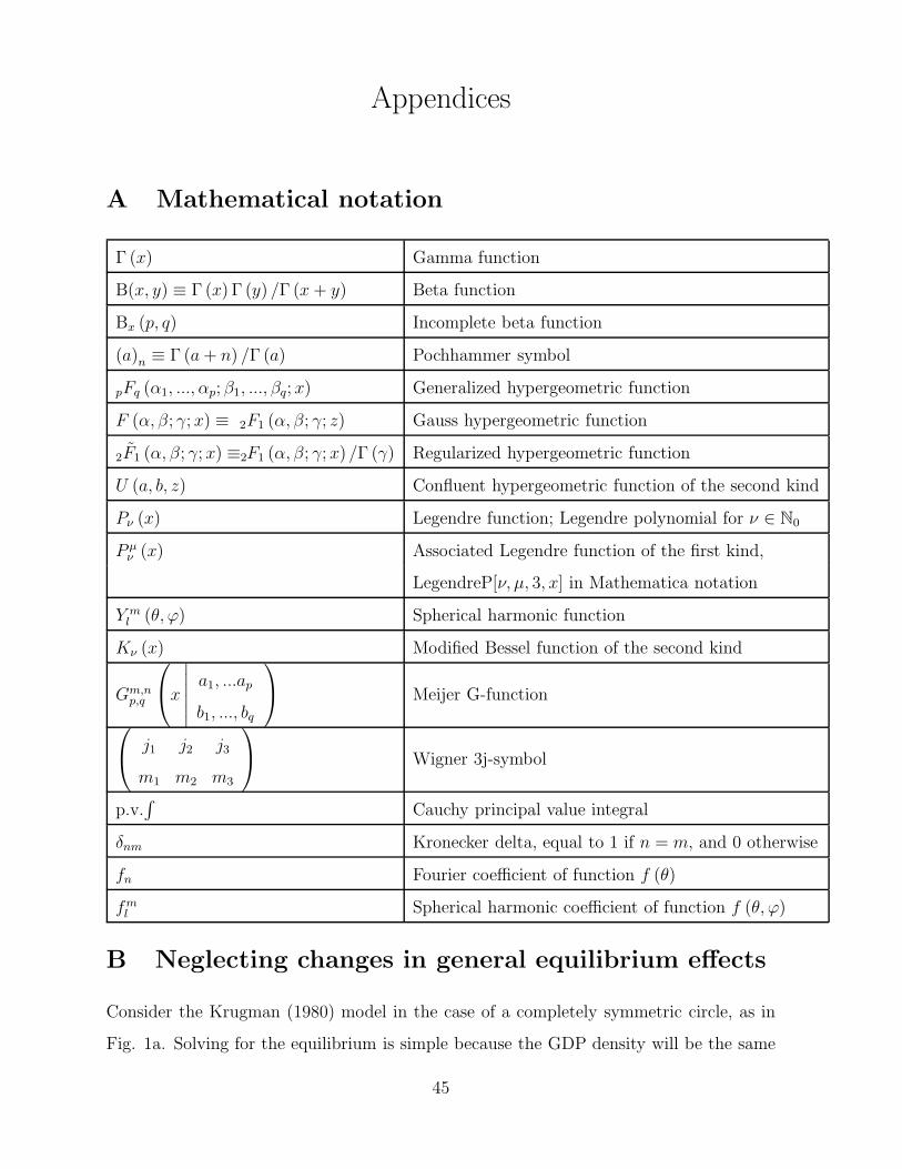
Trade and Interdependence in a Spatially Complex World ⇤ Michal Fabinger † Pennsylvania State University November 13, 2012 Abstract This paper presents an analytic solution framework applicable to a wide vari- ety of general equilibrium international trade models, including those of Krugman (1980), Eaton and Kortum (2002), Anderson and van Wincoop (2003), and Melitz (2003), in multi-location cases. For asymptotically power-law trade costs and in the large-space limit, it is shown that there are parameter thresholds where the qualitative behavior of the model economy changes. In the case of the Krugman (1980) model, the relevant parameter is closely related to the elasticity of substitu- tion between di↵erent varieties of goods. The geographic reach of economic shocks changes fundamentally when the elasticity crosses a critical threshold: below this point shocks are felt even at long distances, while above it they remain local. The value of the threshold depends on the approximate dimensionality of the spatial configuration. This paper bridges the gap between empirical work on international and intranational trade, which frequently uses data sets involving large numbers of locations, and the theoretical literature, which has analytically examined solu- tions to the relevant models with realistic trade costs only for the case of very few locations. ⇤ I am grateful to Mark Aguiar, Manuel Amador, James Anderson, Pol Antr` as, Lorenzo Caliendo, Arnaud Costinot, Dave Donaldson, Jon Eaton, Gita Gopinath, Elhanan Helpman, Oleg Itskhoki, Marc Melitz, Nathan Nunn, Andr´ es Rodrguez-Clare, Robert Townsend, Jim Tybout, Glen Weyl, and Steve Yeaple for extremely helpful discussions, and to seminar participants for very useful comments. † Email: [email protected]
Transcript
Trade and Interdependence
in a Spatially Complex World⇤
Michal Fabinger†
Pennsylvania State University
November 13, 2012
Abstract
This paper presents an analytic solution framework applicable to a wide vari-ety of general equilibrium international trade models, including those of Krugman(1980), Eaton and Kortum (2002), Anderson and van Wincoop (2003), and Melitz(2003), in multi-location cases. For asymptotically power-law trade costs and inthe large-space limit, it is shown that there are parameter thresholds where thequalitative behavior of the model economy changes. In the case of the Krugman(1980) model, the relevant parameter is closely related to the elasticity of substitu-tion between di↵erent varieties of goods. The geographic reach of economic shockschanges fundamentally when the elasticity crosses a critical threshold: below thispoint shocks are felt even at long distances, while above it they remain local. Thevalue of the threshold depends on the approximate dimensionality of the spatialconfiguration. This paper bridges the gap between empirical work on internationaland intranational trade, which frequently uses data sets involving large numbersof locations, and the theoretical literature, which has analytically examined solu-tions to the relevant models with realistic trade costs only for the case of very fewlocations.
⇤I am grateful to Mark Aguiar, Manuel Amador, James Anderson, Pol Antras, Lorenzo Caliendo,Arnaud Costinot, Dave Donaldson, Jon Eaton, Gita Gopinath, Elhanan Helpman, Oleg Itskhoki, MarcMelitz, Nathan Nunn, Andres Rodrguez-Clare, Robert Townsend, Jim Tybout, Glen Weyl, and SteveYeaple for extremely helpful discussions, and to seminar participants for very useful comments.
Imagine that there are two large neighboring countries and that the costs of moving
goods across their shared border changes. How far from the border is the economic
impact going to be felt? Do such changes mostly a!ect regions close to the border, or
do they significantly a!ect even very distant locations? What if productivity increases
or decreases in one of these countries, due to an economic boom or due to a crisis? How
is the productivity change going to influence the level of welfare at various places in the
other country?
To address these questions, it is natural to employ standard models of international
trade, such as Krugman (1980). The solutions to these models have been theoretically
analyzed for some cases. If there are just two or three locations where economic activity
takes place, the analysis is very straightforward.1 To gain insight into situations with many
locations, the theoretical literature has used certain analytically convenient specifications
of trade costs. Apart from zero trade costs, the most popular assumption corresponds
to ‘symmetric trade costs’, in which case the cost of trade between any pair of distinct
locations is the same.2 For example, the multilateral trade policy analysis in Baldwin et
al. (2005) builds on this assumption.
For the present purposes, however, it is necessary to work in a multi-location setting
with more realistic trade costs. Clearly, the transportation costs should grow with dis-
tance. At the same time, they should reflect economies associated with shipping goods
over long distances: the per-unit-distance transportation cost should be a decreasing
function of distance.3
The empirical literature has been working with trade models at this level of realism for
a long time. In recent years, the multi-location aspect has become prominent in empirical
work. Due to falling costs of information technology, highly spatially disaggregated data
1Matsuyama (1999) solves interesting cases with as many as eight locations in the context of themodel introduced in Section 10.4 of Helpman and Krugman (1987), which adds a costlessly tradablehomogeneous good to Krugman (1980).
2In the context of economic geography models (see Fujita et al. (1999)), trade costs exponential indistance proved to be a convenient choice. In that specification, the per-unit-distance trade cost is anincreasing function of distance.
3See Anderson and van Wincoop (2004) and Hummels (2001) for empirical evidence on trade costs.
2
sets are becoming available for empirical analysis. For example, Hillberry and Hummels
(2008) study manufacturers’ shipments within the United States with 5-digit zip code
precision. Compared to previous studies this is a remarkable improvement in spatial
resolution.
The aim of the present paper4 is to bridge the gap between the context in which
international trade models are used for empirical purposes and the context in which they
are studied theoretically. The article introduces a mathematical framework5 that allows
one to solve and analyze such trade models in basic cases involving many locations. The
model discussed extensively is that of Krugman (1980), but this choice is made primarily
for expositional purposes. The models of Anderson and van Wincoop (2003)/Armington
(1969)6 or Melitz (2003) have a very similar mathematical structure,7 and only minor
modifications are needed to write down their solutions once the solutions to the Krugman
model are known. The same is true8 for the Ricardian model of Eaton and Kortum (2002).
This method may also be applied to many other types of trade models, such as those in
Baldwin et al. (2005), where some factors of production are frequently assumed to be
mobile.
What are the practical lessons coming from the analysis? Take the Krugman model
as a representative example. Let the transportation costs be of the ‘iceberg’ type and
asymptotically power-law9 in distance, as commonly assumed in the empirical literature.
Suppose also that the spatial geometry is very large and homogeneously populated. In this
case, it turns out, the way general equilibrium e!ects spread through the economy depends
very strongly on the elasticity of substitution between di!erent varieties of goods. When
the elasticity is above a certain threshold, disturbances spread through the economy by
short-distance interactions. With the elasticity below the threshold, interactions between
4The final version of this paper will include additional discussion of the intuition behind certaintechnical step and results, omitted in the current version due to temporal constraints. The paper will becontinuously updated at http://www.people.fas.harvard.edu/˜fabinger/papers.html
5The framework makes extensive use of standard tools of functional analysis. In the concrete examplesconsidered, these are Fourier series expansion and spherical harmonic expansion.
6The model of Anderson and van Wincoop (2003) is an extension of Armington (1969) and Anderson(1979).
7See Arkolakis et al. (forthcoming) for a detailed analysis of the similarities between the models.8Also the portfolio choice model of Okawa and van Wincoop (2010) has the same property.9For a clarification of the term ‘asymptotically power-law,’ see Subsection 4.3.
3
economic agents separated by long distances play a crucial role. This fact has important
consequences for various quantities of interest.
Consider the case of two large neighboring countries mentioned earlier, and suppose
that the cost associated with moving goods across the border increases slightly. If the
elasticity is above the threshold, only locations close to the border will be a!ected. On the
other side of the threshold, the change in the border cost significantly a!ects all locations.
In the case of a productivity change in one of the countries, the situation is similar. With
the elasticity above the threshold, the e!ects on the other country will be restricted to a
small region close to the border. For the elasticity below the threshold, the consequences
of the productivity change will be felt throughout the other country.
At the empirical level, these observations imply that when fitting a similar trade
model to the data, the usual practice of assuming that all di!erentiated goods have the
same elasticity of substitution can lead to unexpectedly strong biases. The properties
of the model are highly non-linear in the elasticity. Under such circumstances, replacing
heterogeneous goods with a single type of good having the average elasticity is misleading.
A related kind of bias arises when the elementary regions in the data set do not have the
same size. The range of goods contributing to the observed trade flows strongly depends
on the size of each elementary region, leading to a spatial version of selection bias.
The existence of the threshold arises from the interplay between the economic struc-
ture of the model and its spatial properties. It is not something that two-, three-, or
four-location cases would reveal. The value of the threshold is closely tied to the dimen-
sionality10 of the spatial configuration. If the spatial geometry is roughly one-dimensional,
meaning that economic agents are arranged along a line or a circle, the threshold lies at one
particular value for the elasticity of substitution. If economic agents are spread through
a two-dimensional geometry, the value of the threshold is significantly higher.
The solution method used here is easy to generalize to more complex situations. For
example, even though the focus of this paper is on static models, dynamic models can be
10The value of the threshold is a linear function of the dimension of space. It is meaningful to considerzero-dimensional cases as well. This corresponds to spatial configurations with just a few (point-like)locations. Here the threshold condition translates into the requirement that the elasticity of substitutionbe equal to 1. In this case the utility function becomes Cobb-Douglas, which is known to exhibit behaviorqualitatively di!erent from the cases with elasticity of substitution greater than 1.
4
solved11 in a similar fashion. Adding uncertainty does not represent an obstacle, nor does
the addition of di!erentiated goods with di!erent elasticities of substitution.
The present paper is related to two overlapping strands of economic12 research. The
first one is concerned with various aspects of empirical data on trade flows (which are
generally consistent with the ‘gravity model of trade’). The analysis here is most closely
connected to the four models of Krugman (1980), Eaton and Kortum (2002), Melitz
(2003), and Anderson and van Wincoop (2003)/Armington (1969), each associated with
empirical literature13 too rich to explicitly cite here.
The other strand of related research studies the influence of international borders
on trade flows (McCallum (1995), Anderson and van Wincoop (2003), Behrens et al.
(2007), Rossi-Hansberg (2005)) and on price fluctuations (Engel and Rogers (1996),
Gorodnichenko and Tesar (2009), Gopinath et al. (forthcoming)).
The rest of the paper is organized as follows. The next section justifies the use of
functional analysis in later parts of the paper by discussing various pitfalls associated
with oversimplified approaches to multi-location economies. Section 3 reviews the basics
of the representative example of choice, namely the Krugman (1980) model. It also
introduces certain concepts needed to characterize the comparative statics of the model.
Section 4 provides a formal (first-order) solution to the model in the form of an infinite
series. Section 5 uses Fourier series expansion to derive an explicit general solution to the
model in the case of a circular geometry. The resulting formula is then used to analyze
two special cases: the impact of changes in border costs in Section 6, and changes in
productivity in Section 7. Spherical geometry is discussed in Section 8, with spherical
harmonic expansion playing the role of the Fourier series expansion. Section 9 considers
the structure of higher-order terms. In addition to the appendices included in the paper,
there is an online appendix14 providing detailed derivations of certain results, as well as
11The solutions will appear in Fabinger (2011).12There is also a close link to the physics literature; see Section 9 and Appendix L.13Recent examples include Helpman et al. (2004) and Helpman et al. (2008). In the context of the
present paper, it is worth noting that Alvarez and Lucas (2007) establish important properties of theEaton and Kortum (2002) model and provide a basis for solving the model numerically. In addition,they solve the model analytically under the assumption of zero trade costs and under the assumption of‘symmetric trade costs’ mentioned earlier.
14The current (incomplete) version is available at http://www.people.fas.harvard.edu/˜fabinger/papers.html
5
a discussion of additional examples of interest.
2 Challenges of multi-location models
Di!erentiated goods models, as well as a certain type of Ricardian models, typically lead
to large non-linear systems of equations.15 The number of equations as well as the number
of unknowns is proportional to the number of locations considered. It is clearly desirable
to be able to theoretically analyze the solutions to these models even when there is a
large number of locations. However, with realistic16 trade costs this represents a technical
challenge. Even after (log)-linearization the behavior of the system is far from obvious.
The equations become linear,17 which certainly is a simplification, but the number of
equations and unknowns is not reduced. To solve the system, one needs to invert a large
matrix, which is an obstacle18 for the analytic approach.
The present paper uses methods of functional analysis to overcome this di"culty. The
reader may ask whether it is really necessary to go through all the calculations in order
to get a correct picture of the economic phenomena. Could it be that certain shortcuts
lead to qualitatively correct results? The rest of the section is devoted to two such
possibilities: working with a few locations only (Subsection 2.1) and neglecting indirect
general equilibrium interdependencies (Subsection 2.2).
2.1 Working with only a few locations
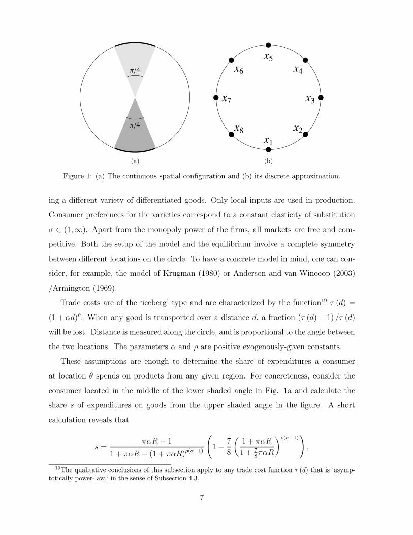
Let us look at a very simple situation in which economic activity takes place at many
di!erent locations. In this example, the physical space is a continuous circle parametrized
by the angle ! ! ("", "]. At every point, there are profit-maximizing firms, each produc-
15An example may be found in Section 3, eq. (3), where each equation links the GDP at a particularlocation to the GDP elsewhere in the economy. This particular case corresponds to Krugman (1980), butanalogous equations for other models have a very similar structure.
16The term ‘realistic trade costs’ here refers to trade costs that increase with distance, but not as fastas to make the per-unit-distance cost also increasing in distance, as discussed in the introduction.
17For trade models where already the exact equations are linear, see Baldwin et al. (2005). An exampleis the ‘footlose capital’ model of Martin and Rogers (1995).
18Cramer’s rule, which expresses the solution to a linear system of equations in terms of a ratio ofdeterminants, is of little help here. The determinants are so complicated that they provide little insightinto the nature of the solution.
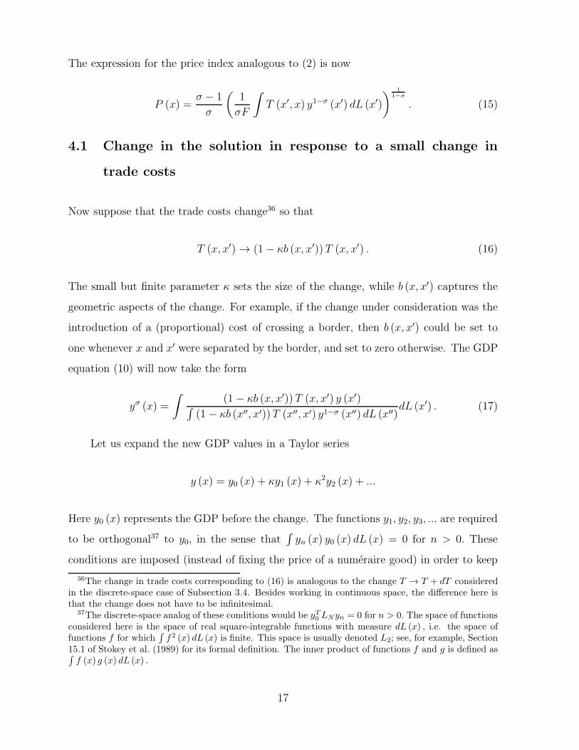
6
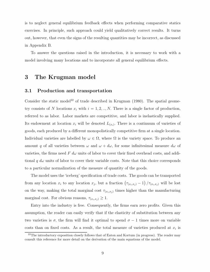
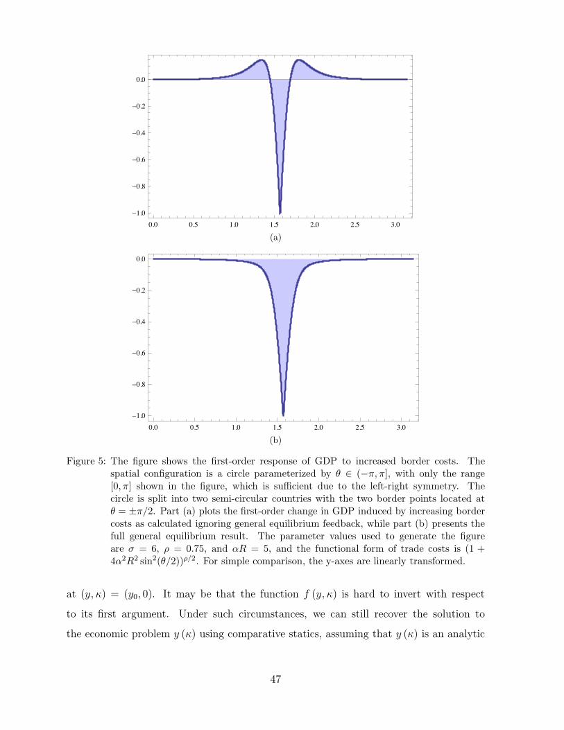
!!4
!!4
(a)
x1x2
x3
x4x5
x6
x7
x8
(b)
Figure 1: (a) The continuous spatial configuration and (b) its discrete approximation.
ing a di!erent variety of di!erentiated goods. Only local inputs are used in production.
Consumer preferences for the varieties correspond to a constant elasticity of substitution
# ! (1,#). Apart from the monopoly power of the firms, all markets are free and com-
petitive. Both the setup of the model and the equilibrium involve a complete symmetry
between di!erent locations on the circle. To have a concrete model in mind, one can con-
sider, for example, the model of Krugman (1980) or Anderson and van Wincoop (2003)
/Armington (1969).
Trade costs are of the ‘iceberg’ type and are characterized by the function19 $ (d) =
(1 + %d)!. When any good is transported over a distance d, a fraction ($ (d)" 1) /$ (d)
will be lost. Distance is measured along the circle, and is proportional to the angle between
the two locations. The parameters % and & are positive exogenously-given constants.
These assumptions are enough to determine the share of expenditures a consumer
at location ! spends on products from any given region. For concreteness, consider the
consumer located in the middle of the lower shaded angle in Fig. 1a and calculate the
share s of expenditures on goods from the upper shaded angle in the figure. A short
calculation reveals that
s ="%R" 1
1 + "%R" (1 + "%R)!("!1)
!
1"7
8
"
1 + "%R
1 + 78"%R
#!("!1)$
,
19The qualitative conclusions of this subsection apply to any trade cost function ! (d) that is ‘asymp-totically power-law,’ in the sense of Subsection 4.3.
7
where R is the radius of the circle. In the large-radius limit, the expression for s simplifies.
limR"#
s =
%
&
'
1"(
78
)1!!("!1)for & (# " 1) < 1,
0 for & (# " 1) > 1.(1)
Now suppose that we approximate the circle with a small and fixed number of locations,
say eight, as in Fig. 1b. If the radius of the circle is very large, consumers at x1 find
varieties produced at other locations very expensive relative to those from x1. They will
spend almost all of their income on local products. As a result, the counterpart20 of s
approaches zero as R $ # even when & (# " 1) < 1.
This line of reasoning leads to the conclusion that it is impossible to qualitatively
reproduce the correct result (1) with a finite and fixed number of locations.21 It is worth
emphasizing that the word ‘fixed’ is important in the last sentence. The behavior of the
continuous model may be reproduced with a discrete one. To do that, one has to increase
the number of locations properly with the radius of the circle when taking the large-space
limit. In other words, there is nothing special about working with a continuum of locations
from the beginning. What is responsible for the failure of the few-location model is not
the discreteness of space, but the fact that additional locations are not added when the
radius of the circle is increased.
2.2 Neglecting changes in general equilibrium e!ects
We have seen that one simple way of avoiding algebraic complications, namely working
with only a few locations, leads to an impasse. Another way to circumvent the di"culty
20In the discrete approximation, there is just one location, namely x5, at the position of the uppershaded angle of the continuous case. For this reason, the discrete counterpart of s is the share ofexpenditures of consumers at x1 on products from x5.
21The reader may ask whether it is possible to make the few-location model correctly reproduce thequalitative behavior of the continuous model by a simple modification of its assumptions. What if weassume that even goods produced and consumed at the same location have to travel a certain distance,say one-half of the spacing between neighboring locations? It turns out that such assumption does notlead to the desired outcome. It is true that for " (# " 1) < 1 the counterpart of s will be non-zero in thelarge-space limit. However, under the same assumption the limit of the counterpart of s remains largeeven in the case " (# " 1) > 1. Moreover, the magnitude of the deviation from (1) depends strongly onthe arbitrary choice of the number of locations in the discrete model. The departure from the correctvalue is attenuated only if the number of locations is chosen to be large, contradicting the purpose of theapproximation.
8
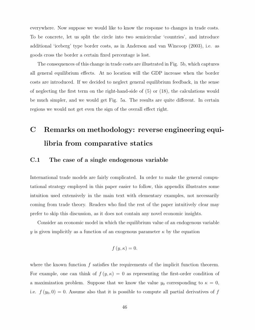
is to neglect general equilibrium feedback e!ects when performing comparative statics
exercises. In principle, such approach could yield qualitatively correct results. It turns
out, however, that even the signs of the resulting quantities may be incorrect, as discussed
in Appendix B.
To answer the questions raised in the introduction, it is necessary to work with a
model involving many locations and to incorporate all general equilibrium e!ects.
3 The Krugman model
3.1 Production and transportation
Consider the static model22 of trade described in Krugman (1980). The spatial geome-
try consists of N locations xi with i = 1, 2, .., N. There is a single factor of production,
referred to as labor. Labor markets are competitive, and labor is inelastically supplied.
Its endowment at location xi will be denoted L(xi). There is a continuum of varieties of
goods, each produced by a di!erent monopolistically competitive firm at a single location.
Individual varieties are labelled by ' ! #, where # is the variety space. To produce an
amount q of all varieties between ' and ' + d', for some infinitesimal measure d' of
varieties, the firms need F d' units of labor to cover their fixed overhead costs, and addi-
tional q d' units of labor to cover their variable costs. Note that this choice corresponds
to a particular normalization of the measure of quantity of the goods.
The model uses the ‘iceberg’ specification of trade costs. The goods can be transported
from any location xi to any location xj , but a fraction(
$(xi,xj) " 1)
/$(xi,xj) will be lost
on the way, making the total marginal cost $(xi,xj) times higher than the manufacturing
marginal cost. For obvious reasons, $(xi,xj) % 1.
Entry into the industry is free. Consequently, the firms earn zero profits. Given this
assumption, the reader can easily verify that if the elasticity of substitution between any
two varieties is #, the firm will find it optimal to spend # " 1 times more on variable
costs than on fixed costs. As a result, the total measure of varieties produced at xi is
22The introductory exposition closely follows that of Eaton and Kortum (in progress). The reader mayconsult this reference for more detail on the derivation of the main equations of the model.
9
H(xi) =1"F L(xi) in this case.
3.2 Consumption
The per-capita consumer utility at a particular location is given by
u =
"*
q!!1! (') d'
#!
!!1
,
where q (') represents the per capita consumption of variety ', # > 1 is the elasticity
of substitution, and the integral is over all varieties available. The per capita spending
p (') q (') on variety ' is given by
p (') q (') =
"
p (')
P
#1!"
c.
Here p (') denotes the price of variety ', the per capita consumption expenditure is
c =+
p (') q (') d', and the local price index P is defined as
P =
"*
p1!" (') d'
#1
1!!
.
To avoid terminological complications, each person is endowed with one unit of labor, and
per capita and per unit labor quantities coincide. GDP per capita will be denoted y, to
be consistent with the notation for consumption per capita.
3.3 Closing the model
The GDP23 y(xi)L(xi) at location xi is equal to the revenue its firms collect from the
measure 1"F L(xi) of varieties they produce,
y(xi) =1
#F
N,
j=1
"
p(xi,xj)
P(xj)
#1!"
c(xj)L(xj).
23Note that local wages are equal to the local GDP per capita, because labor is the only factor ofproduction and firms earn zero profits.
10
Here p(xi,xj) is the price firms from xi charge at xj . Setting the markup p(xi,xj)/(
$(xi,xj)y(xj)
)
to its optimal value of #/ (# " 1) and imposing budget constraints y(xj) = c(xj), the equa-
tion becomes
y(xi) =1
#F
"
#
# " 1
#1!" N,
j=1
"
y(xi)$(xi,xj)
P(xj)
#1!"
y(xj)L(xj),
with the price index given as
P(xj) =#
# " 1
!
1
#F
,
k
$ 1!"(xk,xj)
y1!"(xk)
L(xk)
$1
1!!
. (2)
Combining the last two equations yields
y"(xi) =N,
j=1
$ 1!"(xi,xj)
y(xj)L(xj)-N
k=1 $1!"(xk,xj)
y1!"(xk)
L(xk)
. (3)
This is a set of N equations that must hold in equilibrium, and together they deter-
mine the economic outcome. The choice of units in which y is measured is arbitrary.24
We are free to pick a numeraire good and normalize its price to 1. (In the subsequent
discussion, a di!erent, more abstract condition will be imposed, in order to keep the
calculations simple.)
3.4 Comparative statics - part 1
The rest of the section discusses the comparative statics of the Krugman model, moti-
vates the definition of the GDP propagator, and establishes its basic properties. Readers
interested primarily in the concrete results of the paper, not in their detailed derivation,
may proceed to Section 4.
Consider a small change in trade costs,25 with the goal of evaluating the induced
change in GDP at di!erent places. For ease of notation, denote T(xi,xj) & $ 1!"(xi,xj)
. This
24The set of equations (3) is homogeneous in y.25The general method employed in this paper is elucidated using simple examples in Appendix C.
11
quantity is sometimes referred to as freeness of trade. The GDP equations are
y(xi) =
!
N,
j=1
T(xi,xj)y(xj)L(xj)-N
k=1 T(xk,xj)y1!"(xk)
L(xk)
$1!
. (4)
Suppose we know y corresponding to some particular T . We are interested in the change
y $ y + dy caused by a change T $ T + dT. Here y &(
y(x1), ..., y(xN )
)$and T is a
collection of T(xi,xj). The standard prescription for deriving first-order comparative statics
is to di!erentiate both sides of the equation, leading to
dy(xi) =N,
i=1
G(xi,xj)L(xj)dy(xj) +N,
i=1
N,
j=1
N,
k=1
H(xi,xj,xk)dT(xj,xk). (5)
Here L(xj)G(xi,xj) is the derivative of the right-hand side of the ith equation (4) with
respect to y(xj), and H(xi,xj ,xk) is its derivative with respect to T(xj,xk). In matrix notation,
the set of equations above becomes
(1"GLN) dy =N,
j=1
N,
k=1
H(xj ,xk)dT(xj,xk), (6)
with the N'N matrix G containing elements G(xi,xj), and with the N -dimensional vectors
H(xj ,xk) &(
H(x1,xj,xk), ..., H(xN ,xj ,xk)
)$. The diagonalN'N matrix LN &diag
(
L(x1), ..., L(xN )
)
contains the labor endowments of individual locations on the diagonal. The elements of
all of these objects can be computed explicitly if y is known.
The next standard step is to use these equations to express dy in terms of dT(xj,xk).
To achieve that, one may be tempted to multiply both sides of (6) by (1"GLN )!1 ,
but the situation requires more caution because such matrix is not well-defined. The
homogeneity of eq. (3) implies26 that GLN has one eigenvalue equal to 1, associated with
the eigenvector y: GLNy = y. Consequently, 1 " GLN has a vanishing eigenvalue and
cannot be inverted. For this reason, let us pause here to discuss other properties of the
matrix G, which will enable us to complete the calculation.
26If eq. (4) is satisfied for some vector y, it must also be satisfied for $y, where $ is a positive number.Replacing y by $y in (4), di!erentiating with respect to $, and setting $ = 1 leads to the conclusion thatGLNy = y.
12
3.5 The GDP propagator
Performing the di!erentiation of the right-hand side of (4), G(xi,xj) can be written as a
sum of two parts,
G(xi,xj) = Gc,(xi,xj) +Gp,(xi,xj), (7)
with
Gc,(xi,xj) &1
#y1!"(xi)
T(xi,xj)-N
k=1 T(xk,xj)y1!"(xk)
L(xk)
,
Gp,(xi,xj) &# " 1
#y1!"(xi)
y!"(xj)
N,
l=1
T(xi,xl)y(xl)T(xj ,xl)L(xl).
-Nk=1 T(xk,xl)y
1!"(xk)
L(xk)
/2
= # (# " 1)1
y(xj)
N,
l=1
Gc,(xi,xl)Gc,(xj ,xl)y(xl)L(xl).
The matrix G will be referred to as the GDP propagator,27 and Gc and Gp are its ‘con-
sumption part’ and ‘production part’, respectively. These objects capture the strength of
GDP spillovers from one location to another.
The intuition behind these expressions is simple. The GDP at location xj will a!ect the
GDP at xi through two di!erent channels. The first channel relates to the consumption
at xj , and corresponds to Gc,(xi,xj). Location xi is influenced by the consumption at xj
since firms from xi have customers there. If GDP increases at xj , the firms will receive
more revenue. This is the reason why Gc,(xi,xj) is positive. The second channel is more
closely related to the production at xj , and is captured by Gp,(xi,xj). Firms from xi compete
with firms from xj for customers elsewhere. Higher y(xj) means more expensive products
from xj , raising the revenue that firms from xi receive at xl. This is again a positive
e!ect, translating into a positive Gp,(xi,xj). The first e!ect is direct, so Gc,(xi,xj) contains
T(xi,xj). The second e!ect is indirect, mediated through a third location xl. For this reason
Gp,(xi,xj) contains T(xi,xl)T(xj ,xl) with l being summed over. The presence of the T s in the
denominators is related to the ‘multilateral resistance’ terms in the corresponding ‘gravity
27The algebraic framework used in this paper is an adaptation of the technique of Feynman diagrams,which has become ubiquitous in physics. The term ‘propagator’ is borrowed from that literature.
13
equation’, whose importance has been emphasized by Anderson and van Wincoop (2003).
Notice that if trade costs are not symmetric (in the sense that T(xi,xj) (= T(xj ,xi)),
then the matrix G(xi,xj) will not in general be symmetric. (Even if y(xi) is the same
everywhere and Gp,(xi,xj) is symmetric as a consequence, the consumption part Gc,(xj ,xi)
of the propagator can still be asymmetric.)
The N -dimensional vector space to which y belongs can be thought of as a one-
dimensional space spanned by y times an (N " 1)-dimensional vector space YN!1 whose
elements y satisfy yTLN y = 0. We already know that the action of GLN preserves the one
dimensional space: GLNy = y. But it is also true28 that the (N " 1)-dimensional space
YN!1 is preserved by the action of this matrix. (In other words, if yTLN y = 0, then also
yTLN (GLN y) = 0.)
Because both the space YN!1 and the space spanned by the vector y are preserved by
the action of GLN , the matrix GLN may be written as
GLN = Pspan{y}GLNPspan{y} +PYN!1GLNPYN!1
= Pspan{y} +PYN!1GLNPYN!1
, (8)
where Pspan{y} is the projector onto the one-dimensional space generated by the vector y,
and PYN!1is the projector onto YN!1.
3.6 Comparative statics - part 2
Now let us go back to the discussion of (6). We have not imposed any normalization
condition on y+dy yet. The international trade literature typically chooses a definite good
to serve as numeraire, and normalizes its price to 1. Such choice would be inconvenient in
the present context. To take advantage of the decomposition (8), we need to impose the
more abstract29 condition yTLNdy = 0, i.e. dy ! YN!1. It follows that GLNdy ! YN!1,
28To verify this property, it is su"cient to show thatGTLNy = ay for some constant a.Direct evaluationusing the expressions for Gc,(xi,xj) and Gp,(xi,xj) above confirms that this is indeed the case with a = 1,i.e. that GTLNy = y.
29If all elements of the vector y have the same magnitude, this condition translates into the requirementthat the total (nominal) GDP remain fixed as the trade costs change. More generally, the quantity keptfixed is a weighted average of the GDP at individual locations. The same condition may be interprettedin terms of wages, since these are identically equal to the GDP per capita in this model.
14
and as a result of (6), also that-N
j=1
-Nk=1H(xj ,xk)dT(xj,xk) ! YN!1. Thanks to these
properties, the equation (6) can be written as
PYN!1(1"GLN )PYN!1
dy =N,
j=1
N,
k=1
H(xj ,xk)dT(xj,xk).
Since dy and the right-hand side of this equation belong to YN!1, andPYN!1(1"GLN)PYN!1
is an operator on YN!1, we can restrict attention to that space and conclude that30
dy =.
PYN!1(1"GLN)PYN!1
/!1N,
j=1
N,
k=1
H(xj ,xk)dT(xj,xk). (9)
Here, of course, the inversion is performed in YN!1, not in the full N -dimensional space.
As discussed in Subsection 3.4, GLN has one eigenvalue equal to 1 and associated with
the eigenvector y. Stability of the system implies that all other eigenvalues are smaller
than 1 in absolute value. For this reason PYN!1(1"GLN )PYN!1
is invertible in YN!1,
and the final expression for dy is well-defined.
4 The Krugman model in continuous space
While introductory exposition is simpler with a finite number of locations, the exam-
ples discussed below will involve continuous space. Retaining a fine discrete grid in the
model would not lead to any additional economic insights, and the continuous-space ex-
amples provide greater algebraic convenience. The equations of the model may easily be
translated into continuum notation.
Let the spatial geometry be a continuous space with points parametrized by a vector of
coordinates x. In general, the space can be curved. The coordinates are chosen arbitrarily.
30The continuous-space analog of this equation is the relation (21) in Section 4.
15
Denote the labor element31 at location x by dL (x) . The equation (3) for GDP becomes
y" (x) =
*
T (x, x$) y (x$)+
T (x$$, x$) y1!" (x$$) dL (x$$)dL (x$) , (10)
where T (x, x$) & $ 1!" (x, x$) . The degree of interdependence between di!erent locations
is captured by the GDP propagator32 defined33 as
G (x, x$) = Gc (x, x$) +Gp (x, x
$) , (11)
with the ‘consumption part’
Gc (x, x$) =
1
#
y1!" (x) T (x, x$)+
y1!" (x$$) T (x$$, x$) dL (x$$), (12)
and the ‘production part’
Gp (x, x$) = # (# " 1)
1
y (x$)
*
Gc (x, x$$)Gc (x
$, x$$) y (x$$) dL (x$$) . (13)
Intuitively, the GDP propagator G (x, x$) measures how strongly an infinitesimal change
in GDP at x$ influences the GDP at x. The consumption part reflects the fact that if
consumption at x$ increases, this will directly increase the sales of firms from x. The
production part arises from the fact that increased GDP (wages) at x$ make it easier for
firms from x to compete in other markets.34
The GDP propagator satisfies the conditions35
y (x) =
*
G (x, x$) y (x$) dL (x$) , y (x) =
*
G (x$, x) y (x$) dL (x$) . (14)
31To follow the discussion, the reader does not have to be familiar with various concepts of di!erentialgeometry. Nevertheless, they are useful for expressing dL (x) in more explicit terms. The distances inthe physical space are captured by a definite metric tensor whose values depend on x. Denoting itsdeterminant g (x) , the endowment of labor dL (x) in a particular coordinate element dx equals
0
g (x)dxtimes the labor density.
32As mentioned in Subsection 3.5, the term ‘propagator’ comes from related physics literature.33For the discrete analog of this definition, see eq. (7).34This intuition is discussed in more detail in Subsection 3.5.35These are analogous to the conditions y = GLNy and y = GTLNy of Subsection 3.5.
16
The expression for the price index analogous to (2) is now
P (x) =# " 1
#
"
1
#F
*
T (x$, x) y1!" (x$) dL (x$)
# 11!!
. (15)
4.1 Change in the solution in response to a small change in
trade costs
Now suppose that the trade costs change36 so that
T (x, x$) $ (1" (b (x, x$)) T (x, x$) . (16)
The small but finite parameter ( sets the size of the change, while b (x, x$) captures the
geometric aspects of the change. For example, if the change under consideration was the
introduction of a (proportional) cost of crossing a border, then b (x, x$) could be set to
one whenever x and x$ were separated by the border, and set to zero otherwise. The GDP
Let us expand the new GDP values in a Taylor series
y (x) = y0 (x) + (y1 (x) + (2y2 (x) + ...
Here y0 (x) represents the GDP before the change. The functions y1, y2, y3, ... are required
to be orthogonal37 to y0, in the sense that+
yn (x) y0 (x) dL (x) = 0 for n > 0. These
conditions are imposed (instead of fixing the price of a numeraire good) in order to keep
36The change in trade costs corresponding to (16) is analogous to the change T $ T + dT consideredin the discrete-space case of Subsection 3.4. Besides working in continuous space, the di!erence here isthat the change does not have to be infinitesimal.
37The discrete-space analog of these conditions would be yT0 LNyn = 0 for n > 0. The space of functionsconsidered here is the space of real square-integrable functions with measure dL (x) , i.e. the space offunctions f for which
+
f2 (x) dL (x) is finite. This space is usually denoted L2; see, for example, Section15.1 of Stokey et al. (1989) for its formal definition. The inner product of functions f and g is defined as+
f (x) g (x) dL (x) .
17
the calculations simple. The rationale behind this choice is explained in Subsection 3.6.
The main focus of this paper is on the first-order change y1 (x) . The higher-order terms
yn, n % 2, may be computed in an analogous way. They are the subject of Section 9. An
equation for the first-order term y1 (x) can be obtained by plugging the Taylor expansion
into the GDP equation and comparing terms of the first-order in (. The details of the
calculation can be found in Appendix D. The result is
y1 (x) =
*
G (x, x$) y1 (x$) dL (x$) +
*
B (x, x$) y0 (x$) dL (x$) , (18)
with the ‘primary impact function’ B (x, x$) defined as
B (x, x$) = "b (x, x$)Gc (x, x$) + #Gc (x, x
$)
*
b (x$$, x$)Gc (x$$, x$) dL (x$$) . (19)
Alternatively, using an operator notation, this is
y1 (x) = (Gy1) (x) + (By0) (x) .
In general, for a given function F (x, x$) the action of the corresponding operator F on a
function f will be defined38 as
(Ff) (x) =
*
F (x, x$) f (x$) dL (x$) . (20)
Since y1 is orthogonal to y0, and, due to (14), so is Gy1, it must be that By0 is
orthogonal to y0 as well. The equation for y1 (x) can be iterated indefinitely, giving39
y1 (x) =#,
n=0
(GnBy0) (x) . (21)
38Note that the measure dL (x!) used here corresponds to the labor endowment. The discrete-spaceanalog would be multiplication by the matrix FLN .
39The discrete-space counterpart of this equation is the relation (9). When interpreting the result (21)for y1, it is useful to compare it to the expression (60) in Appendix C, which applies to the case of twoendogenous variables. Obviously, the function By0 plays the role of the vector v. It is an initial e!ectof the change in %. Just like in (60), this e!ect has an infinite number of echoes, described by the termsGnBy0 with positive n.
18
Here we used the identity40 limn"#Gny1 = 0. For later convenience, let us define also the
‘general equilibrium GDP propagator’41 Gg (x, x$) as the integral kernel of the operator
Gg = "#,
n=0
Gn+1. (22)
In terms of Gg, the result (21) becomes
y1 (x) = ((1 +Gg)By0) (x) .
Another useful expression for y1 may obtained using the identity B = " (1" #Gc) Gc,
which follows from the definition (19) of B. Here Gc is the integral operator corresponding
to
Gc (x, x$) & Gc (x, x
$) b (x, x$) . (23)
Denoting also
gc (x) &*
Gc (x, x$) dL (x$) , (24)
we havey1y0
= " (1 +Gg) (1" #Gc) gc. (25)
For future convenience, let us also introduce the notation
gc (x) &*
Gc (x$, x) dL (x$) . (26)
Of course, if Gc (x, x$) b (x, x$) = Gc (x$, x) b (x$, x) in general, then gc (x) = gc (x) .
The intuition behind the expression (19) for the primary impact function B (x, x$) is as
follows. If a new trade barrier, say a border, is introduced between x and x$, such change
is captured by positive b (x, x$) . There will be two immediate e!ects on x. First, with the
new barrier, firms from x will lose some part of their revenues from x$. This lowers y (x)
and is consistent with the first term in (19) being negative. Second, it will be easier for
40This follows from the fact that any Gny1 is orthogonal to y0, thanks to (14), and from the factthat all eigenvalues of G are smaller than 1 in absolute value, except for the one corresponding to theeigenfunction y0.
41This object captures not only the direct interdependencies, but also all the general equilibriumfeedback e!ects.
19
these firms to compete with firms from x$$ in the market at x$, as long as b (x$$, x$) is also
positive. This e!ect increases y (x). For this reason, the second term in (19) is positive.
4.2 Welfare
The welfare of individual agents is characterized by the local GDP per capita adjusted for
the local price index, y(P ) (x) & y (x) /P (x), where the price index P (x) is given by (15)
with the replacement T (x$, x) $ (1" (b (x$, x))T (x$, x) . Appendix E shows that the
price-index-adjusted analog of y1 (x) , namely y(P )1 (x) & lim#"0
.
y(P ) (x)" y(P )0 (x)
/
/(,
is given by
y(P )1 (x)
y(P )0 (x)
=y1 (x)
y0 (x)" #
*
Gc (x$, x)
y1 (x$)
y0 (x$)dL (x$)"
#
# " 1gc (x) , (27)
or, in operator notation,
y(P )1
y(P )0
= (1" #Gc)y1y0
"#
# " 1gc. (28)
Here gc is the function defined in (26).
4.3 Asymptotically power-law transportation costs
Before specializing to concrete economic situations, let us pause here to clarify the choice
of trade cost functions that will be used in the rest of the paper. The Krugman model
uses the ‘iceberg’ form of trade costs, characterized by the quantity $ (x, x$) . In principle,
the trade costs can depend on many characteristics of location pairs. For example, they
are likely to be lower when the two locations share a common language. The present work
will abstract from many such possibilities. Instead, the trade costs will take the simple
form
$ (x, x$) = $ (d) b (x, x$) .
The first factor $ (d) corresponds to transportation costs, and depends only on the distance
d between x and x$. The second factor b (x, x$) represents additional costs, such as the cost
20
of crossing international borders. In baseline cases without any additional trade costs,
b (x, x$) will be set to 1.
It is common in the empirical literature42 to assume that for large d, $ (d) is well
approximated by a power law:
$ (d) ) (%d)! ,
with & > 0 and % > 0. Of course, $ (d) cannot be exactly equal to (%d)! at short distances.
Otherwise the obvious restriction $ (d) % 1 would be violated43 for small enough d. There
are several convenient functional forms that ensure the $ % 1 restriction is satisfied while
preserving the power-law behavior at long distances, for example (1 + %2d2)"2 , (1 + %d)! ,
or 1 + (%d)! . The present article works with finite geometries, such as a circle or a
sphere of radius R. In these cases, closely related functional forms(
1 + 4%2R2 sin2 d2R
)"2 ,
(
1 + 2%R sin d2R
)!, and 1+
(
%R sin dR
)!provide a greater algebraic convenience. At short
distances, these coincide with the previous three, while at long distances they still have
the same order of magnitude.
For future purposes, let us mention one important property of the six functional forms
above. Define the function $ (d) as
$ (d) &
%
&
'
1 for d * 1$ ,
(%d)! for d % 1$ .
It is true that for each of the six functional forms $ (d) considered above, there exist44
positive constants al and ah independent of R such that
al$ (d) * $ (d) * ah$ (d) (29)
for all d ! [0, "R]. Loosely speaking, this means that these $ (d) are similar to the simple
function $ (d) . In general, monotonic functions satisfying this condition will be referred
42See, for example, Anderson and van Wincoop (2003).43Unless b (x, x!) is chosen to precisely compensate for the small magnitude of ! (d) whenever x and x!
are close to each other.44Concrete values of these coe"cients {al, ah} that can be used for the functional forms
to as ‘asymptotically power-law’, despite the fact that the geometries under consideration
have finite R. In the large R limit, the term ‘asymptotically’ regains its conventional
meaning.
To simplify notation in the rest of the paper, the following combination of & and #
will be denoted ):
) &1
2& (# " 1) .
5 The Krugman model on the circle
5.1 Basic setup
Consider the case where the spatial geometry is a circle45 of radius R with points parametrized
by ! ! ("", "], and where the labor density is constant. Identify the coordinate x with !.
The labor element is now dL (!) = &Ld! with &L = L/ (2") . The endowment of labor per
unit of physical length is &L/R. A baseline solution to the Krugman model corresponding
to $ (!, !$) = $ (d) is easy to obtain. Due to rotational symmetry, the GDP equation
is solved by setting the GDP density to a constant, y0 (!) = y0. The GDP propagator
G (!, !$) associated with this solution depends only on the distance d (!, !$) between its
arguments, defined as the smaller of |! " !$| and 2" " |! " !$| . For this reason, all the
information in G (!, !$) can be captured by a function G with only one argument defined
by G (d (!, !$)) = G (!, !$) . This specifies the single-argument G (!) only for ! ! [0, "] . For
notational convenience, extend it symmetrically to negative arguments, G ("!) = G (!),
and then periodically over the entire real line, G (! + 2"n) = G (!) , n ! Z. The action
(20) of the operator G on any (periodically extended) function f (!) on the circle can be
written as
(Gf) (!) = &L (G + f) (!) = &L
* %
!%
G (! " !$) f (!$) d!$. (30)
Define also the single argument functions Gc (!), Gp (!), and Gg (!) in a similar way. The
symbol + here stands for a 2"-periodic convolution. For any two 2"-periodic functions f
45The case of a finite number of locations symmetrically arranged on a circle can be solved in a similarfashion, employing discrete Fourier tranform instead of Fourier series expansion.
22
and g their 2"-periodic convolution is defined as
(f + g) (!) =* %
!%
f (! " !$) g (!$) d!$.
In the context of the circular geometry, the term ‘convolution’ will always refer to the
2"-periodic convolution.
5.2 Expansion in terms of convolution powers of Gc (!)
We will see that the numerical values of the solutions y1 can have very di!erent orders
of magnitude depending on the values of the parameters of the model, such as & or
#. It is desirable to have an intuitive way of finding the correct order of magnitude
without performing explicit calculations. For this purpose, let us take a closer look at
the mathematical objects the solution contains. Readers interested primarily in the final
results for y1, not in the properties of individual contributions to it, may proceed to the
next subsection.
The formal solution (21) can be written as
y1 =#,
n=0
&nLG%n + (By0) , (31)
where the nth convolution power G%n (!) of G (!) is the n-fold (2"-periodic) convolution
of the function G (!) with itself. Because equations (11) and (13) imply G (!) = Gc (!) +
# (# " 1) &LG%2c (!) , the expression for y1 can be written as
y1 =#,
n=0
&nL(
Gc + # (# " 1) &LG%2c
)%n + (By0) . (32)
We see that the right-hand side is a linear combination of various convolution powers
G%mc of the function Gc, convoluted with the function By0. In order to gain some intuition
about the behavior of y1 for large R, it is necessary understand what the functions G%mc
look like in that case.
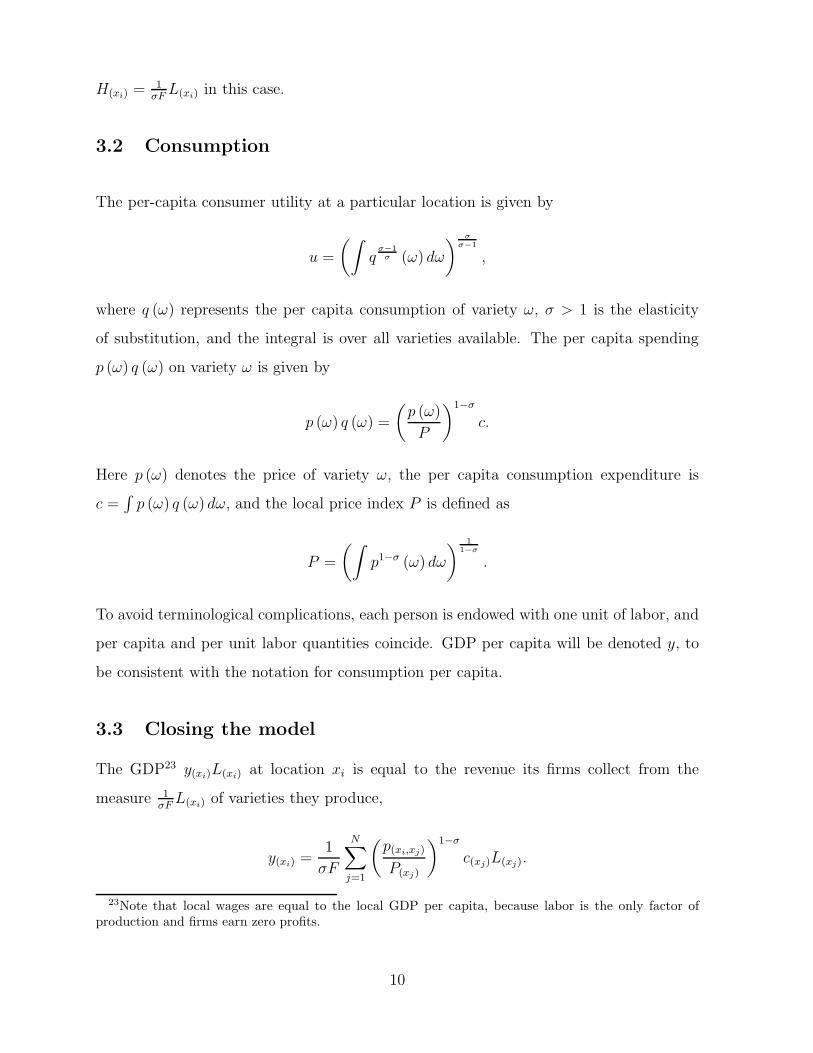
5.2.1 The large R limit of G%2c (!) and G%m
c (!) with m % 3
23
Suppose that R is very large, much larger than 1/%. The assumption of asymptotically
power-law trade costs (29) has implications for the behavior of the function G%2c (!) &
+ %
!% Gc (!$)Gc (! " !$) d!$. A few of its properties are immediately clear. We know that
Gc (!) is a positive decreasing function of |!| ! [0, "] . As a consequence, the same must
be true for G%2c (!) . Also, decreasing ) & & (# " 1) /2 increases the importance of the tails
of the function Gc (!), and makes it more spread out. This means that relative to Gc (!),
any features of the function G%2c (!) will be even more smoothed out. (Note that these
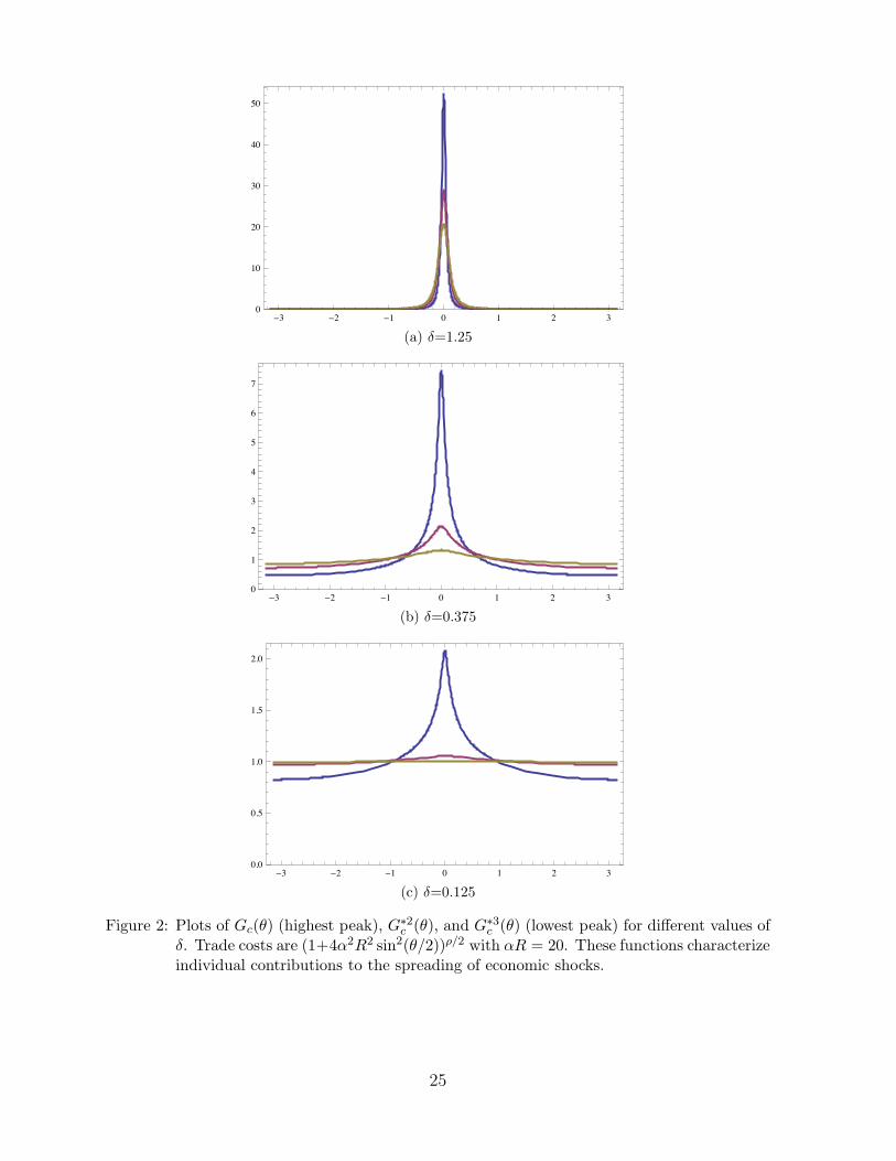
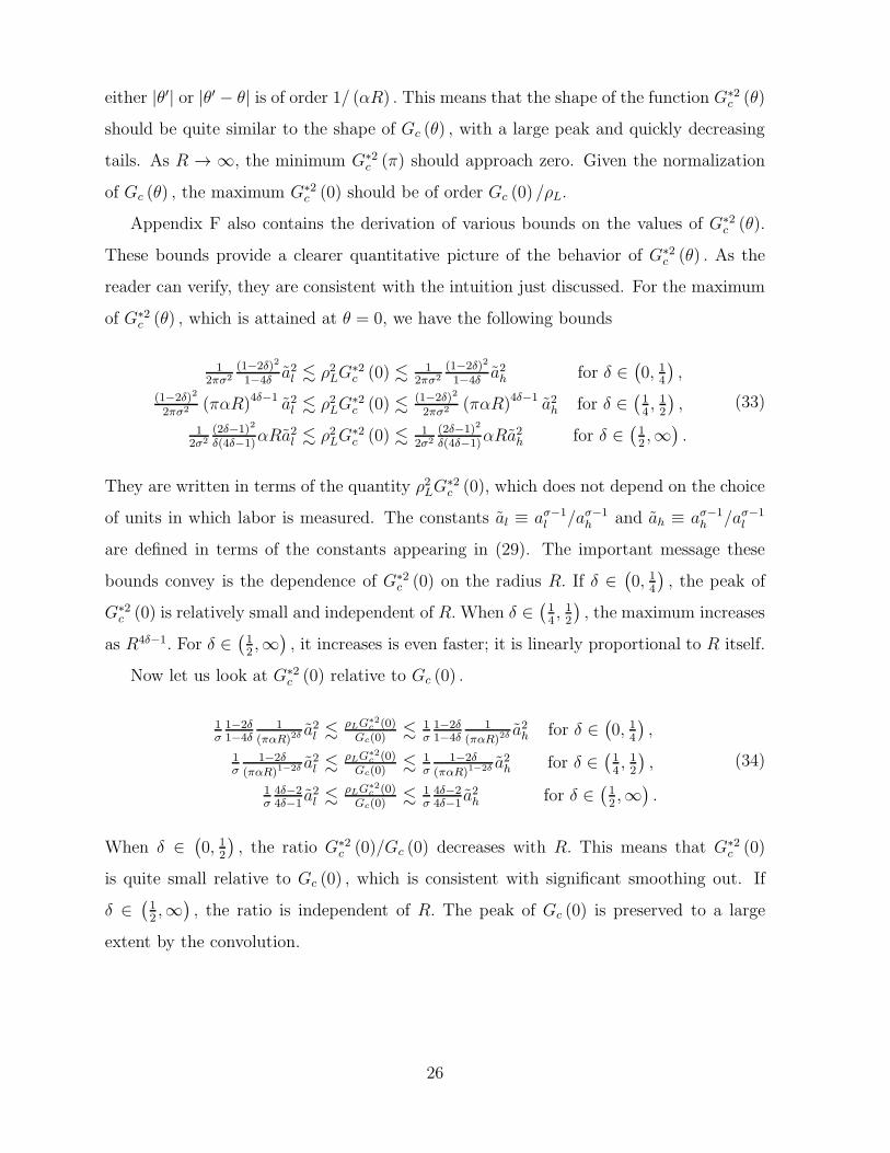
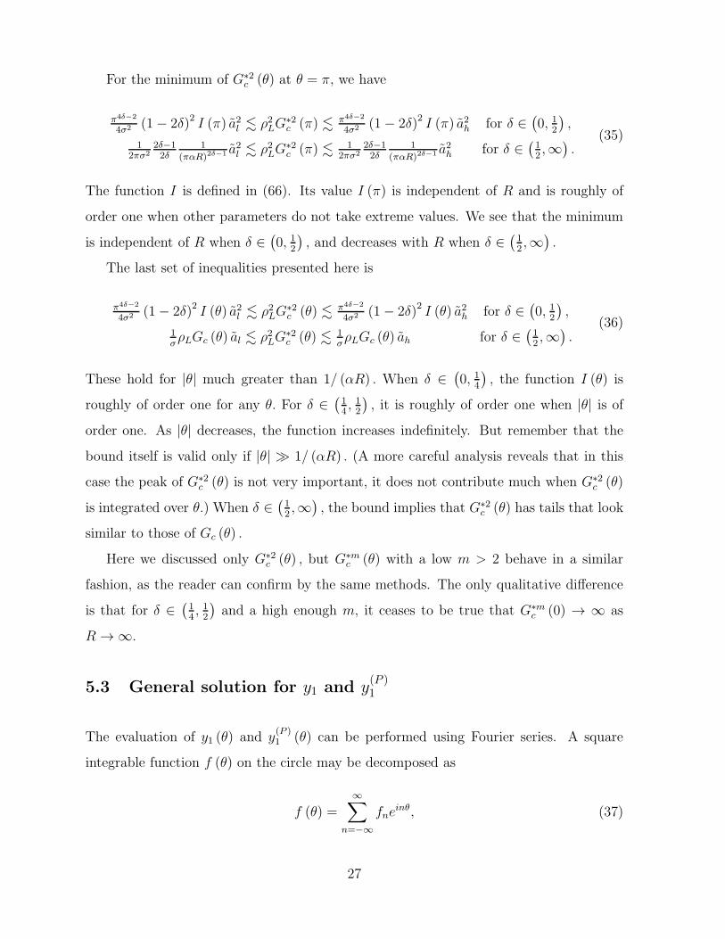
observations, as well as those that follow, are consistent with the plots in Fig. 2.)
In order to gain a more detailed intuitive understanding of the properties of G%2c (!),
it is important to know which regions of the integration domain dominate the integral.
This issue is technical, and for this reason the derivations are left for Appendix F, but
the results follow. For ) !(
0, 14)
, the main contribution to the integral comes from |!$|
and |! " !$| being both of order one. For ) !(
14 ,
12
)
it comes from |!$| of order |!| . When
) !(
12 ,#
)
, the integral is dominated by the region where |!$| is of order 1/ (%R) and the
region where |!$ " !| is of order 1/ (%R) .
With this knowledge one can make an informed guess about the shape of G%2c (!) .
With ) !(
0, 14)
, the integral is insensitive to what happens at short distances of order
1/ (%R) . For this reason, even though Gc (!) has a relatively sharp peak, this feature will
be smoothed out in the case of G%2c (!) . One can expect the maximum G%2
c (0) to be of
the same order of magnitude as the minimum G%2c (") . Moreover, G%2
c (") should have a
finite positive limit as R $ #.
For ) !(
14 ,
12
)
, the situation is a little more subtle. For |!| of order one, the integral
is still dominated by long distances, i.e. by |!$| and |! " !$| of order one. One would
therefore expect the minimum G%2c (") to take similar values as in the previous case. It
should stay finite and positive as R $ #. By contrast, for small |!|, say of order 1/ (%R),
the integral is dominated by short distances, i.e. by |!$| and |! " !$| of order 1/ (%R) .
This contribution is larger than the contribution of long distances, and as a consequence
there should be a substantial peak at ! = 0. In other words, G%2c (0) , G%2
c (") .
When ) !(
12 ,#
)
, the story is again relatively simple. Irrespective of the value of !,
the dominant contribution to the integral comes from the short-distance regions, where
24
"3 "2 "1 0 1 2 30
10
20
30
40
50
(a) (=1.25
"3 "2 "1 0 1 2 30
1
2
3
4
5
6
7
(b) (=0.375
"3 "2 "1 0 1 2 30.0
0.5
1.0
1.5
2.0
(c) (=0.125
Figure 2: Plots of Gc()) (highest peak), G%2c ()), and G%3
c ()) (lowest peak) for di!erent values of(. Trade costs are (1+4&2R2 sin2()/2))!/2 with &R = 20. These functions characterizeindividual contributions to the spreading of economic shocks.
25
either |!$| or |!$ " !| is of order 1/ (%R) . This means that the shape of the function G%2c (!)
should be quite similar to the shape of Gc (!) , with a large peak and quickly decreasing
tails. As R $ #, the minimum G%2c (") should approach zero. Given the normalization
of Gc (!) , the maximum G%2c (0) should be of order Gc (0) /&L.
Appendix F also contains the derivation of various bounds on the values of G%2c (!).
These bounds provide a clearer quantitative picture of the behavior of G%2c (!) . As the
reader can verify, they are consistent with the intuition just discussed. For the maximum
of G%2c (!) , which is attained at ! = 0, we have the following bounds
12%"2
(1!2&)2
1!4& a2l ! &2LG%2c (0) ! 1
2%"2(1!2&)2
1!4& a2h for ) !(
0, 14
)
,
(1!2&)2
2%"2 ("%R)4&!1 a2l ! &2LG%2c (0) ! (1!2&)2
2%"2 ("%R)4&!1 a2h for ) !(
14 ,
12
)
,
12"2
(2&!1)2
&(4&!1)%Ra2l ! &2LG%2c (0) ! 1
2"2(2&!1)2
&(4&!1)%Ra2h for ) !(
12 ,#
)
.
(33)
They are written in terms of the quantity &2LG%2c (0), which does not depend on the choice
of units in which labor is measured. The constants al & a"!1l /a"!1
h and ah & a"!1h /a"!1
l
are defined in terms of the constants appearing in (29). The important message these
bounds convey is the dependence of G%2c (0) on the radius R. If ) !
(
0, 14)
, the peak of
G%2c (0) is relatively small and independent of R. When ) !
(
14 ,
12
)
, the maximum increases
as R4&!1. For ) !(
12 ,#
)
, it increases is even faster; it is linearly proportional to R itself.
Now let us look at G%2c (0) relative to Gc (0) .
1"1!2&1!4&
1(%$R)2#
a2l !!LG"2
c (0)Gc(0)
! 1"1!2&1!4&
1(%$R)2#
a2h for ) !(
0, 14
)
,
1"
1!2&(%$R)1!2# a2l !
!LG"2c (0)
Gc(0)! 1
"1!2&
(%$R)1!2# a2h for ) !(
14 ,
12
)
,
1"4&!24&!1 a
2l !
!LG"2c (0)
Gc(0)! 1
"4&!24&!1 a
2h for ) !
(
12 ,#
)
.
(34)
When ) !(
0, 12)
, the ratio G%2c (0)/Gc (0) decreases with R. This means that G%2
c (0)
is quite small relative to Gc (0) , which is consistent with significant smoothing out. If
) !(
12 ,#
)
, the ratio is independent of R. The peak of Gc (0) is preserved to a large
extent by the convolution.
26
For the minimum of G%2c (!) at ! = ", we have
%4#!2
4"2 (1" 2))2 I (") a2l ! &2LG%2c (") ! %4#!2
4"2 (1" 2))2 I (") a2h for ) !(
0, 12)
,
12%"2
2&!12&
1(%$R)2#!1 a2l ! &2LG
%2c (") ! 1
2%"22&!12&
1(%$R)2#!1 a2h for ) !
(
12 ,#
)
.(35)
The function I is defined in (66). Its value I (") is independent of R and is roughly of
order one when other parameters do not take extreme values. We see that the minimum
is independent of R when ) !(
0, 12)
, and decreases with R when ) !(
12 ,#
)
.
The last set of inequalities presented here is
%4#!2
4"2 (1" 2))2 I (!) a2l ! &2LG%2c (!) ! %4#!2
4"2 (1" 2))2 I (!) a2h for ) !(
0, 12)
,
1"&LGc (!) al ! &2LG
%2c (!) ! 1
"&LGc (!) ah for ) !(
12 ,#
)
.(36)
These hold for |!| much greater than 1/ (%R) . When ) !(
0, 14
)
, the function I (!) is
roughly of order one for any !. For ) !(
14 ,
12
)
, it is roughly of order one when |!| is of
order one. As |!| decreases, the function increases indefinitely. But remember that the
bound itself is valid only if |!| , 1/ (%R) . (A more careful analysis reveals that in this
case the peak of G%2c (!) is not very important, it does not contribute much when G%2
c (!)
is integrated over !.) When ) !(
12 ,#
)
, the bound implies that G%2c (!) has tails that look
similar to those of Gc (!) .
Here we discussed only G%2c (!) , but G%m
c (!) with a low m > 2 behave in a similar
fashion, as the reader can confirm by the same methods. The only qualitative di!erence
is that for ) !(
14 ,
12
)
and a high enough m, it ceases to be true that G%mc (0) $ # as
R $ #.
5.3 General solution for y1 and y(P )1
The evaluation of y1 (!) and y(P )1 (!) can be performed using Fourier series. A square
integrable function f (!) on the circle may be decomposed as
f (!) =#,
n=!#
fnein', (37)
27
where i =-"1 is the imaginary unit and the Fourier coe"cients fn are given by
fn =1
2"
* %
!%
f (!) e!in'd!. (38)
In general, the notation used here for the nth Fourier coe"cients will be to add subscript
n to the symbol of the corresponding function. The convolution theorem for Fourier series
states that for two functions f and g the Fourier coe"cients (f + g)n of their (2"-periodic)
convolution f +g may be computed by multiplying the Fourier coe"cients of the individual
functions,
(f + g)n = 2"fngn.
The operator G acts according to (30) as a convolution with &LG (!), so
(Gf)n = LGnfn.
Identical relations hold also for Gc, Gp, and Gg. In the last case, one should remember
that Gg is only well defined when acting on functions orthogonal to the constant function
y0, i.e. on functions f whose zeroth Fourier coe"cient f0 vanishes.
We can now find an expression for the Fourier coe"cients y1,n of the function y1 (!) .
The zeroth coe"cient y1,0 vanishes since y1 is chosen to be orthogonal to the constant
function y0. For nonzero n, applying the convolution theorem to the general expression
(25) givesy1,ny0
= " (1 + LGg,n) (1" #LGc,n) gc,n.
This can be further simplified by two identities. The first identity, LGg,n = 1/ (1" LGn)"
1, comes from the definition (22), and the standard formula for the sum of a geometric
series. The second identity, LGn = (1 + # (# " 1)LGc,n)LGc,n, is a consequence of (11)
and (13). Together they imply that " (1 + LGg,n) (1" #LGc,n) gc,n = " gc,n1+("!1)LGc,n
. The
conclusion is that
y1,ny0
=
%
&
'
0 for n = 0,
" gc,n1+("!1)LGc,n
for n (= 0.(39)
28
For the local-price-index-adjusted GDP y(P )1 (28) leads to
y(P )1,n
y(P )0
=
%
&
'
" ""!1 gc,0 for n = 0,
" 1!"LGc,n
1+("!1)LGc,ngc,n " "
"!1 gc,n for n (= 0.(40)
If b (!, !$) = b (!$, !) , the Fourier coe"cients are real and gc,n = gc,n. In that case (40)
simplifies to
y(P )1,n
y(P )0
=
%
&
'
" ""!1 gc,0 for n = 0,
"2"!1"!1
gc,n1+("!1)LGc,n
for n (= 0.(41)
5.4 Fourier coe"cients of Gc (!) for specific functional forms of
trade costs
The general formula (12) for Gc (x, x$) reduces in the case under consideration to
Gc (!, !$) = Gc (! " !$) =
1
#&L
T (! " !$)+ %!% T (!$$ " !$) d!$$
=1
#&L
T (! " !$)+ %!% T (!$$) d!$$
. (42)
Here, of course, the T (! " !$) corresponds to the trade costs before the introduction of
border costs, T (! " !$) = $ 1!" (! " !$) . The Fourier coe"cients of Gc (!) are
Gc,n =1
#LT0Tn.
Note that this implies that Gc,0 = 1/ (#L) , and via (11) and (13) also that Gc,0 = 1/L,
as expected from (14).
Subsection (4.3) mentioned several convenient functional forms for transportation
costs. They all have similar properties. For the purpose of finding analytic solutions to the
Krugman model, we will focus mostly on one of them, namely $ (d) =(
1 + 4%2R2 sin2 d2R
)"2 ,
but the other ones can be treated similarly.46 For the functional form of choice, T (!) can
be written as
T (!) =
!
1
1 + 4%2R2 sin2 '2
$&
,
46A discussion of other asymptotically power-law trade costs will be included in a future version of theonline appendix at http://www.people.fas.harvard.edu/˜fabinger/papers.html
29
where the important parameter ) is defined as
) &1
2& (# " 1) .
An alternative expression for T (!) is
T (!) = Z2&
!
1
Z2 cos2 '2 + sin2 '
2
$&
(43)
with
Z2 &1
1 + 4%2R2
As shown in Appendix I, the Fourier coe"cients of T (!) are
Tn =Z& ("1)n
(1" ))nP n&!1
"
1 + Z2
2Z
#
.
P ba (z) is the associated Legendre function.47 The Pochhammer symbol (a)n is defined in
terms of the gamma function as $ (a+ n) /$ (a), and should not be confused with the
notation for Fourier coe"cients. For positive integer n, this definition reduces to the nth
order polynomial (a)n = a (a + 1) (a+ 2) ... (a + n" 1) . The resulting expression for Gc,n
is
Gc,n =1
#L
("1)n
(1" ))n
P n&!1
.
1+Z2
2Z
/
P&!1
(
1+Z2
2Z
) . (44)
6 The impact of border costs
6.1 General solution for GDP in the presence of border costs
Now consider the introduction of a small border cost. Let us split the circle into two
‘countries’, country A characterized by ! !(
"%2 ,
%2
)
and country B by ! !(
"", %2
)
.(%2 , "],
separated by a border consisting of two points, "%2 and %
2 . This assumption is made for
47Mathematica introduces three distinct definitions of associated Legendre functions. The functionused here corresponds to the third definition, i.e. to LegendreP[*,µ,3,z]. See Appendix A for a list ofspecial functions and other mathematical notation.
30
simplicity, and generalization to di!erent situations is straightforward. The trade costs
are now $ (!, !$) = $ (d) b (!, !$), with
b (!, !$) & 1 + (1CA(!) 1CB
(!$) + (1CB(!) 1CA
(!$) ,
where 1CAand 1CB
are the country indicator functions. The small positive parameter (
is related to the parameter ( considered in the general discussion by ( & 1" (1 + ()1!".
For small (, this is roughly ( ) (# " 1) (. In terms of T (!, !$) the change associated with
the introduction of the border cost is T (!, !$) $ (1" (b (!, !$)) T (!, !$) with
b (!, !$) & 1CA(!) 1CB
(!$) + 1CB(!) 1CA
(!$) .
The Fourier coe"cients gc,n of the function gc (!) are given in Appendix H,
gc,n =
%
&
'
0 for n odd,
12")0n "
4(!1)n2
%2
-#m=0
LGc,2m+1
(2m+1)2!n2 for n even.(45)
The result (39) then becomes
y1,ny0
=
%
&
'
0 for n odd or zero,
4(!1)n2
%21
1+("!1)LGc,n
-#m=0
LGc,2m+1
(2m+1)2!n2 for n even and nonzero,
while (41) gives
y(P )1,n
y0=
%
3
3
3
&
3
3
3
'
"12
1"!1 +
4%2
""!1
-#m=0
LGc,2m+1
(2m+1)2for n zero,
4(!1)n2
%22"!1"!1
11+("!1)LGc,n
-#m=0
LGc,2m+1
(2m+1)2!n2 for n even nonzero,
0 for n odd.
(46)
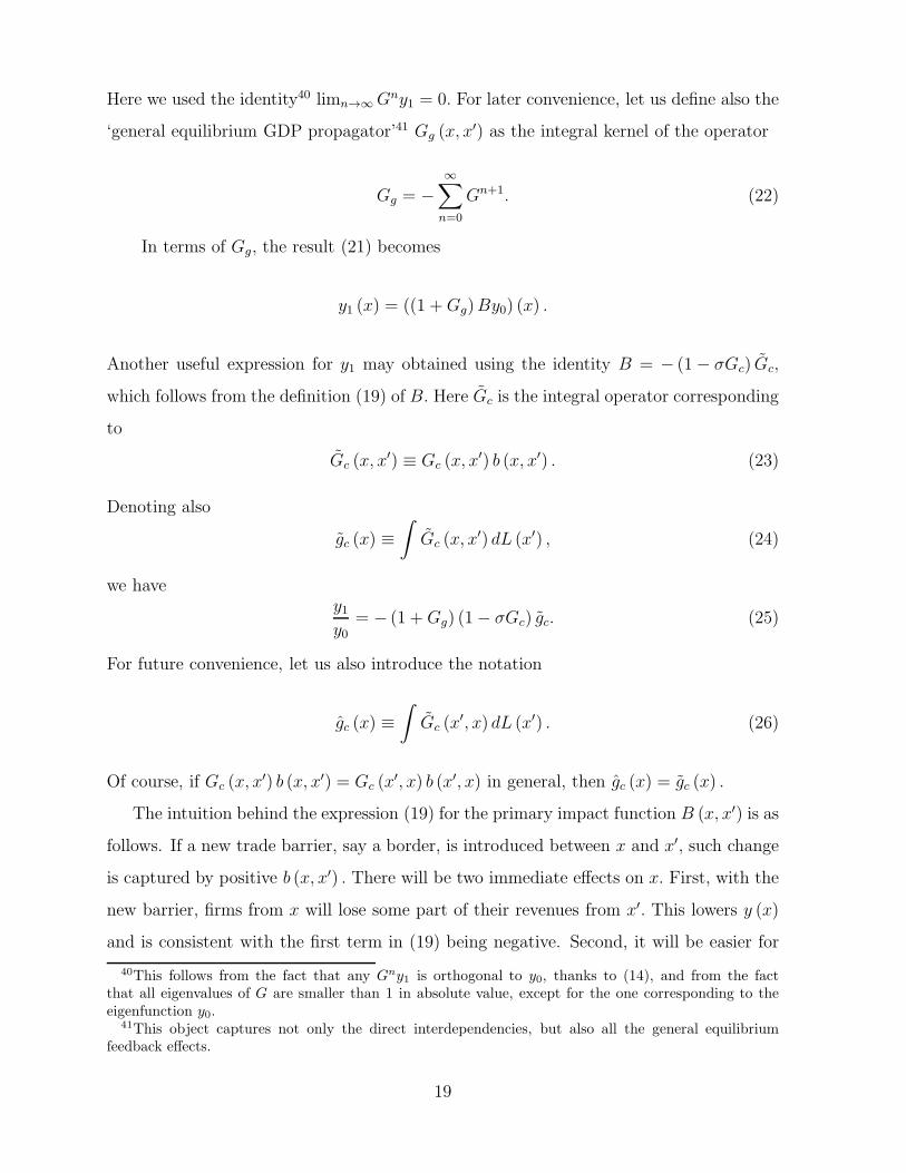
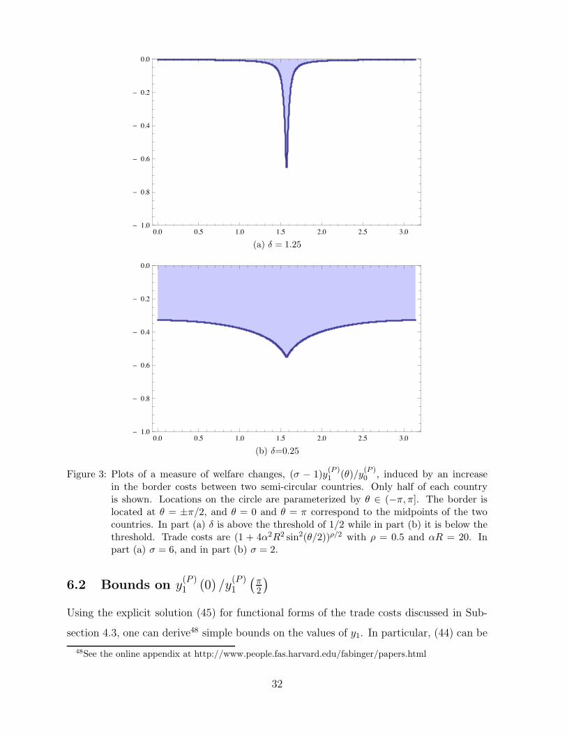
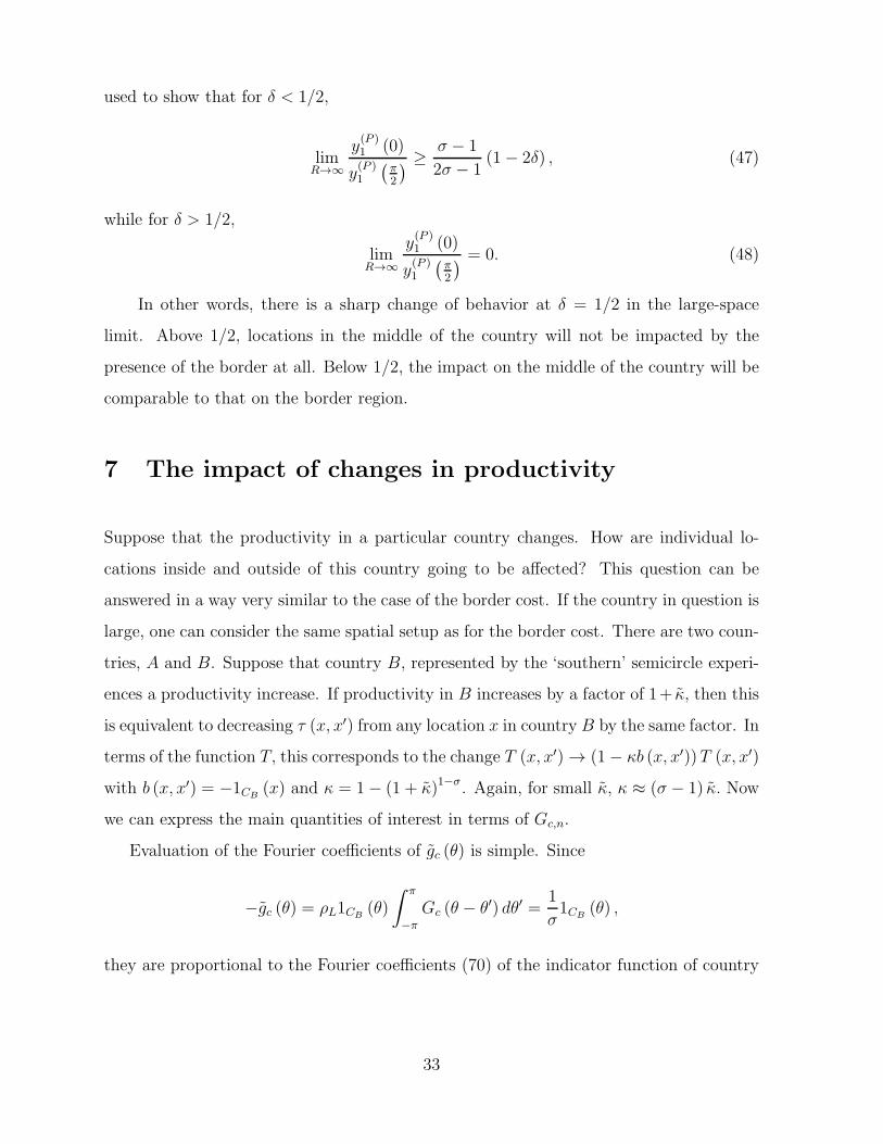
The resulting function y(P )1 (!) is plotted in Fig. 3 for di!erent values of the parameter ).
31
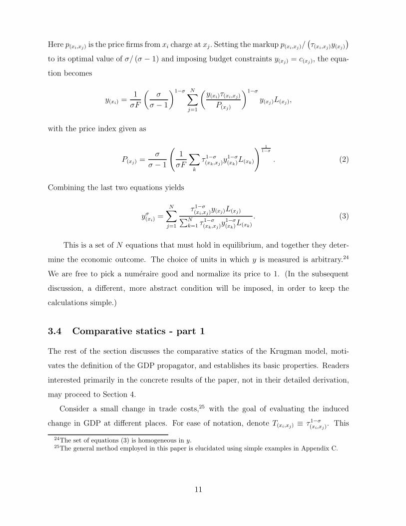
0.0 0.5 1.0 1.5 2.0 2.5 3.0" 1.0
" 0.8
" 0.6
" 0.4
" 0.2
0.0
(a) ( = 1.25
0.0 0.5 1.0 1.5 2.0 2.5 3.0" 1.0
" 0.8
" 0.6
" 0.4
" 0.2
0.0
(b) (=0.25
Figure 3: Plots of a measure of welfare changes, (# " 1)y(P )1 ())/y(P )
0 , induced by an increasein the border costs between two semi-circular countries. Only half of each countryis shown. Locations on the circle are parameterized by ) ! ("',']. The border islocated at ) = ±'/2, and ) = 0 and ) = ' correspond to the midpoints of the twocountries. In part (a) ( is above the threshold of 1/2 while in part (b) it is below thethreshold. Trade costs are (1 + 4&2R2 sin2()/2))!/2 with " = 0.5 and &R = 20. Inpart (a) # = 6, and in part (b) # = 2.
6.2 Bounds on y(P )1 (0) /y(P )
1
(
'2
)
Using the explicit solution (45) for functional forms of the trade costs discussed in Sub-
section 4.3, one can derive48 simple bounds on the values of y1. In particular, (44) can be
48See the online appendix at http://www.people.fas.harvard.edu/fabinger/papers.html
32
used to show that for ) < 1/2,
limR"#
y(P )1 (0)
y(P )1
(
%2
)%
# " 1
2# " 1(1" 2)) , (47)
while for ) > 1/2,
limR"#
y(P )1 (0)
y(P )1
(
%2
)= 0. (48)
In other words, there is a sharp change of behavior at ) = 1/2 in the large-space
limit. Above 1/2, locations in the middle of the country will not be impacted by the
presence of the border at all. Below 1/2, the impact on the middle of the country will be
comparable to that on the border region.
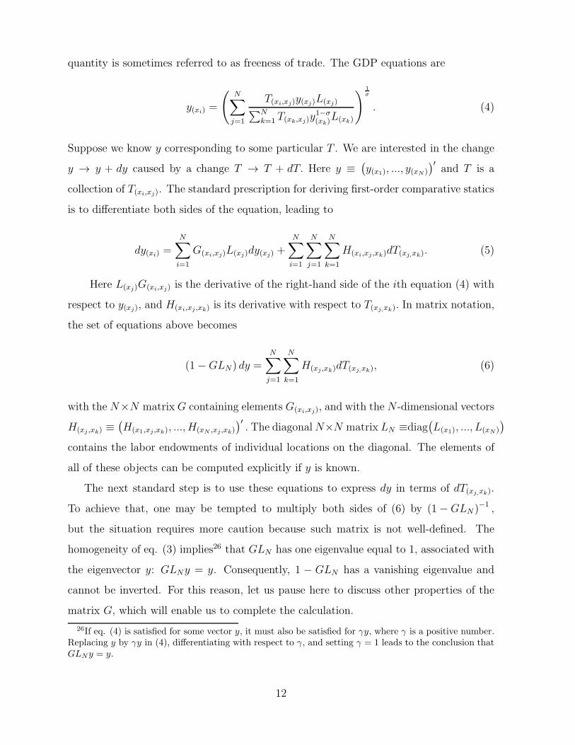
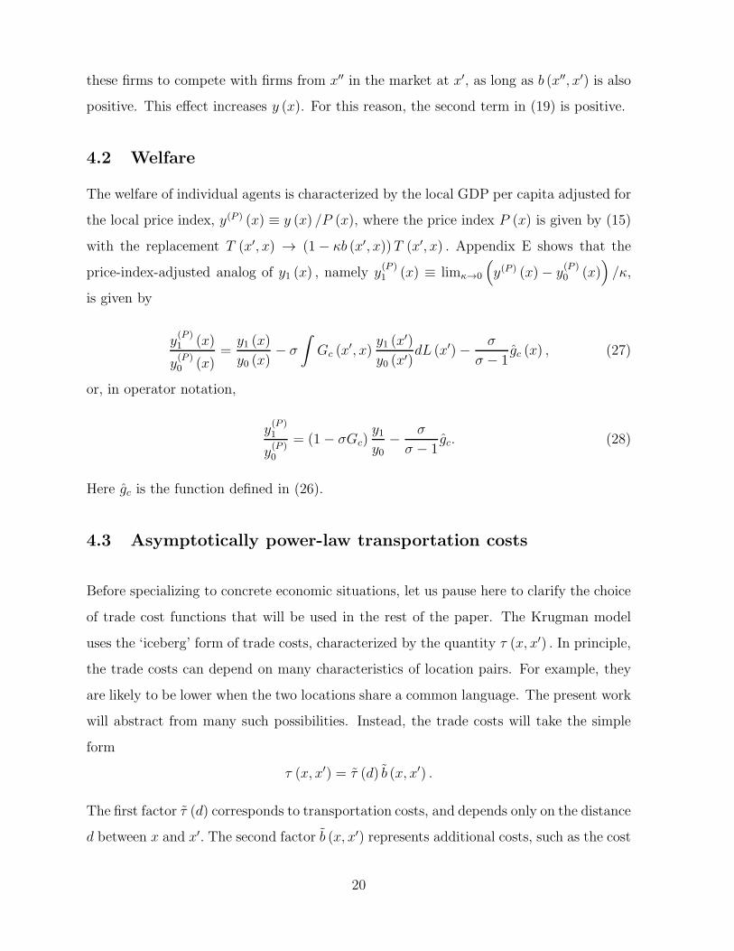
7 The impact of changes in productivity
Suppose that the productivity in a particular country changes. How are individual lo-
cations inside and outside of this country going to be a!ected? This question can be
answered in a way very similar to the case of the border cost. If the country in question is
large, one can consider the same spatial setup as for the border cost. There are two coun-
tries, A and B. Suppose that country B, represented by the ‘southern’ semicircle experi-
ences a productivity increase. If productivity in B increases by a factor of 1+ (, then this
is equivalent to decreasing $ (x, x$) from any location x in country B by the same factor. In
terms of the function T, this corresponds to the change T (x, x$) $ (1" (b (x, x$))T (x, x$)
with b (x, x$) = "1CB(x) and ( = 1" (1 + ()1!". Again, for small (, ( ) (# " 1) (. Now
we can express the main quantities of interest in terms of Gc,n.
Evaluation of the Fourier coe"cients of gc (!) is simple. Since
"gc (!) = &L1CB(!)
* %
!%
Gc (! " !$) d!$ =1
#1CB
(!) ,
they are proportional to the Fourier coe"cients (70) of the indicator function of country
33
0.0 0.5 1.0 1.5 2.0 2.5 3.00.0
0.2
0.4
0.6
0.8
1.0
(a) ( = 1.25
0.0 0.5 1.0 1.5 2.0 2.5 3.00.0
0.2
0.4
0.6
0.8
1.0
(b) (=0.25
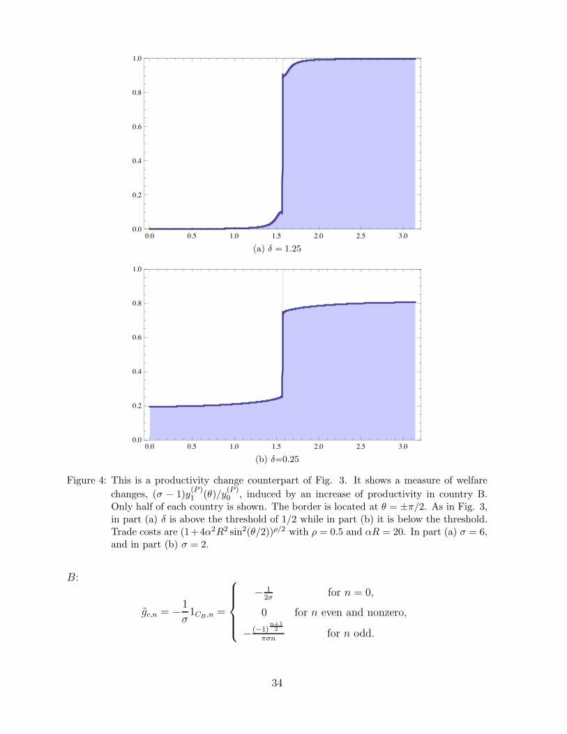
Figure 4: This is a productivity change counterpart of Fig. 3. It shows a measure of welfare
changes, (# " 1)y(P )1 ())/y(P )
0 , induced by an increase of productivity in country B.Only half of each country is shown. The border is located at ) = ±'/2. As in Fig. 3,in part (a) ( is above the threshold of 1/2 while in part (b) it is below the threshold.Trade costs are (1+4&2R2 sin2()/2))!/2 with " = 0.5 and &R = 20. In part (a) # = 6,and in part (b) # = 2.
B:
gc,n = "1
#1CB ,n =
%
3
3
3
&
3
3
3
'
" 12" for n = 0,
0 for n even and nonzero,
" (!1)n+12
%"n for n odd.
34
Substituting these expressions into (39) gives
y1,ny0
=
%
&
'
0 for n even ,
(!1)n+12
%n1
1+("!1)LGc,nfor n odd.
For the local-price-index-adjusted GDP, we should use the general formula (40) instead of
(41), since b (!, !$) is not identically equal to b (!$, !). Remembering that Gc,0 = 1/ (#L) ,
"gc (!) = &L
* !$2
!%
Gc (! " !$) d!$ + &L
* %
$2
Gc (! " !$) d!$
= &L
#,
n=!#
Gc,nein'
!
* !$2
!%
e!in'#d!$ +
* %
$2
e!in'#d!$$
=1
2#+
1
"
#,
n=!#, n odd
("1)n+12
nLGc,ne
in'.
For the individual Fourier coe"cients gc,n this implies
gc,n =
%
3
3
3
&
3
3
3
'
" 12" for n = 0,
0 for n even nonzero,
" (!1)n+12
%n LGc,n for n odd.
The formula (40) then yields
y(P )1,n
y(P )0
=
%
&
'
" ""!1 gc,0 for n = 0,
" 1!"LGc,n
1+("!1)LGc,ngc,n " "
"!1 gc,n for n (= 0.
y(P )1,n
y(P )0
=
%
3
3
3
&
3
3
3
'
12
1"!1 for n = 0,
0 for n even nonzero,
(!1)n+12
%"n
.
1!"LGc,n
1+("!1)LGc,n+ "2
"!1LGc,n
/
for n odd.
See Fig. 4 for plots of y(P )1 for di!erent values of the parameter ). Again, there is a
threshold behavior at ) = 1/2. Bounds analogous to (47) and (48) will be included a
future version of the online appendix.
35
8 The Krugman model on the sphere
8.1 The role of dimensionality
The previous section established that in the large-space limit, the qualitative properties
of the Krugman model on the circle with asymptotically power-law trade costs change as
) & & (# " 1) /2 crosses the threshold of 1/2. This value is not universal, however. For
spaces of di!erent dimensionality, the value of the threshold is di!erent. In general, for a
ds-dimensional space, the threshold condition is49
) =ds2.
Clearly, it is of little economic interest to study cases with ds % 3. The choice ds = 2,
however, is more appropriate for real-world economies than ds = 1.
For this reason, the present section is devoted to the Krugman model on a two-
dimensional spatial geometry, the sphere. It turns out that its properties closely resemble
the case of the circle, apart form the fact that the role of ) is now played by )/2.
8.2 Basic setup
Let the spatial geometry be a sphere S of radius R parameterized by colatitude ! ! [0, "]
and longitude * ! [0, 2"). Identify these coordinates with x introduced previously, x =
(!,*) . As in the case of the circle, labor density is chosen to be constant. The labor
element is dL (!,*) = &L sin !d!d* with &L = L/ (4"). The endowment of labor per unit
physical area equals &LR2. Again, the baseline solution corresponds to constant GDP
density: y0 (!,*) = y0. The GDP propagator G (x, x$) depends only on the (rescaled)
distance d (x, x$) between x and x$ given by
cos d (x, x$) = sin ! sin !$ + cos ! cos !$ sin (*" *$) .
49A hint that this may be the case comes from repeating the calculations that led to eq. (1). A carefulanalysis of geometries of arbitrary dimension provides a confirmation.
36
The information contained in G (x, x$) can be captured by a single-argument function G,
defined by the relation G.
d (x, x$)/
= G (x, x$). The action (30) of the operator G can
be thought of as a spherical convolution with &LG.
d (x, x$)/
,
(Gf) (x) = &L (G + f) (x) = &L
*
S
G.
d (x, x$)/
f (x$) dA (x$) .
Here dA (x$) is the (rescaled) area element at point x$ = (!$,*$) and may be written
as dA (x$) = sin !$d!$d*$. A similar statement holds for Gc, Gp, and Gg and analogously
defined functions Gc(d), Gp(d), and Gg(d). Again, it is worth remembering that the action
of Gg is defined only on functions orthogonal to the constant function y0.
Convolutions on the sphere are a little more subtle than convolutions on the circle. In
the case of the circle there is a natural definition of convolution for arbitrary functions
as long as the corresponding integral is convergent. On the sphere a natural definition
of convolution exists only if at least one of the convolution factors is required to be
rotationally symmetric, in the sense that it depends only on ! but not on *. The functions
G(d), Gc(d), Gp(d) and Gg(d) all satisfy this requirement, so this is not a source of any
di"culty here. The general definition of spherical convolution is
(F + f) (x) =*
S
F.
d (x, x$)/
f (x$) dA (x$) . (49)
Here F is the function that only depends on !, identified with d, and f may depend on
both spherical coordinates of the point x$.
The spherical analogs of (31) and (32) take the same form,
y1 =#,
n=0
&nLG%n + (By0) =
#,
n=0
&nL(
Gc + # (# " 1) &LG%2c
)%n + (By0) .
The large R results for G%2c (!) (and higher G%m
c (!)) for the case of the circle have a direct
analog here. To avoid repetition, detailed discussion is left for Appendix G. As mentioned
earlier, the main lesson is that the role of ) (defined as & (# " 1) /2) in the case of the
circle is now played by )/2. Otherwise the qualitative behavior remains the same.
37
8.3 General solution for y1 and y(P )1
A square integrable function f (!,*) on the sphere can be written as
f (!,*) =#,
l=0
l,
m=!l
fml Y m
l (!,*) , (50)
for some coe"cients fml . These coe"cients may be computed as
fml =
*
S
f (!,*)Y m%l (!,*)
0
g (x)dx =
* %
0
* 2%
0
f (!,*)Y m%l (!,*) d* sin !d!, (51)
where the star denotes complex conjugation. The spherical harmonic function Y ml (!,*)
of degree l and order m is defined as
Y ml (!,*) = N |m|
l P |m|l (cos !) eim(.
P |m|l is the associated Legendre polynomial of degree l and order |m|, i =
-"1 is the
imaginary unit, and N |m|l is a positive normalization factor needed to make the system
orthonormal (without the Condon-Shortley phase). The general convention for spherical
harmonic coe"cients of a function on the sphere is to add the indices l and m to the
corresponding symbol of the function. When the index m is zero, it may be omitted. In
other words, fl & f 0l . All spherical harmonics needed here will be of order zero.50 They
are given more explicitly as
Y 0l (!,*) &
-2l + 1-4"
Pl (cos !) , (52)
where Pl is the Legendre polynomial of degree l. According to the convolution theorem on
the sphere, spherical harmonic coe"cients of the convolution (49) are equal to properly
normalized products of the spherical harmonic coe"cients of the individual convolution
factors:
(F + f)ml =
-4"-
2l + 1Flf
ml , (53)
50In other applications of the same framework, working with spherical harmonics of nonzero order maybe necessary.
38
with Fl & F 0l . For the GDP propagator G this implies
(Gf)ml =1-4"
1-2l + 1
LG0l f
ml ,
and similarly for Gc, Gp and Gg. Following the same steps as in the case of the circle, we
obtain
(y1)ml
y0=
%
&
'
0 for l = 0 or m (= 0,
" gc,l1+("!1) 1$
4$1$2l+1
LGc,lfor l > 0 and m = 0,
(54)
.
y(P )1
/m
l
y(P )0
=
%
3
3
3
&
3
3
3
'
0 for m (= 0,
" ""!1 gc,0 for l = 0 and m = 0,
"&4%
&2l+1!"LGc,l&
4%&2l+1+("!1)LGc,l
gc,l " ""!1 gc,l for l > 0 and m = 0.
(55)
8.4 Solutions for specific functional forms of trade costs
Proceeding in analogy with the case of the circle,
Gc (!,*, !$,*$) = Gc
.
d (!,*, !$,*$)/
=1
#&L
T.
d (!,*, !$,*$)/
+ %0
+ 2%0 T
.
d (!$$,*$$, !$,*$)/
sin !$$d*$$d!$$,
Gc (!) =
-4"
#LT 00
T (!) .
The spherical harmonic coe"cients of Gc (!) are
(Gc)ml =
-4"
#LT 00
Tml .
Note that G00 =
-4"/L, which is consistent with (14). For transportation costs of the
form $ (d) =(
1 + 4%2R2 sin2 d2R
)"2 ,
T (!) = Z2&
!
1
Z2 cos2 '2 + sin2 '
2
$&
,
39
with ) & & (# " 1) /21 and Z2 & (1 + 4%2R2)!1
. Because of rotational symmetry Tml = 0
and (Gc)ml = 0 for m (= 0. As shown in Appendix K, the remaining coe"cients are
Tl = 2"-2l + 1 ())l
Z12+&
-1" Z2
P!l! 1
2
&! 32
"
1 + Z2
2Z
#
,
Gc,l =
-4" ())l#L
P!l! 1
2
&! 32
.
1+Z2
2Z
/
P! 1
2
&! 32
(
1+Z2
2Z
)
.
8.5 The impact of changes in border costs
The spherical counterpart of the two semicircular ‘countries’ are the northern and the
southern hemisphere, CA = {(!,*) |! ! [0, %2 )}, and CB = {(!,*) |! ! (%2 , "]}. The
corresponding spherical harmonic coe"cients of gc (and gc) are given by equation (75)
in Appendix J. The values of the coe"cients can be used in the expressions (54) and
(75) for the change in GDP. The resulting solutions exhibit the threshold behavior at
) = 1. Bounds analogous to (47) and (48) will be included in a future version of the online
appendix.
8.6 The impact of changes in productivity
Similarly to the case of the circle, gc (!,*) equals "1CB(!,*) /#. As a result, its spherical
harmonic coe"cients with non-zero m vanish and the others are proportional to (74):
gc,l =
%
3
3
3
&
3
3
3
'
" 1"
-" for l = 0,
0 for l even and nonzero,
" 1"
-"-2l + 1 (!1)
!l!12
2l(l!1)!
l!12 ! l+1
2 !for l odd.
The formula (54) then gives
(y1)ml
y0=
%
&
'
0 for l even or m (= 0,
1"(!1)
!l!12
2l(l!1)!
l!12 ! l+1
2 !
2%(2l+1)&4%
&2l+1+("!1)LGc,l
for l odd and m = 0.
40
Recognizing that gc (!) = "&L (Gc + 1CB) (!) and applying the spherical convolution the-
orem (53) leads to
gc,l =
%
3
3
3
&
3
3
3
'
" 12" for l = 0,
0 for l even and nonzero,
" (!1)!l!1
2
2l+1(l!1)!
l!12 ! l+1
2 !LGc,l for l odd.
Of course, (gc)ml with nonzero m vanish. The price-index-adjusted change in GDP (55)
becomes
.
y(P )1
/m
l
y(P )0
=
%
3
3
3
3
3
3
&
3
3
3
3
3
3
'
12
1"!1 for l = 0 and m = 0,
0 for l even nonzero or m (= 0,
1"(!1)
!l!12
2l(l!1)!
l!12 ! l+1
2 !
.-"-2l + 1
&4%
&2l+1!"LGc,l&
4%&2l+1+("!1)LGc,l
+ 12
"2
"!1LGc,l
/
for l odd and m = 0.
As in the case of border cost, the qualitative behavior changes at ) = 1. For bounds
analogous to (47) and (48), see a future version of the online appendix.
9 Higher-order terms
The first-order changes in GDP y1 (x) capture the full impact of changes in trade costs
when ( is very small. There is an analytic way to evaluate this impact even for larger
(. The goal of this section is to provide basic insight into how this can be achieved. A
detailed discussion is left for a future version of the online appendix, because this issue
lies outside of the main focus of the paper.
As in Section 4, suppose that there is an initial equilibrium with GDP equal to y0 (x),
and consider a change in trade costs. If the trade costs were characterized initially by
T (x, x$) and after the change by (1" (b (x, x$)) T (x, x$), the new GDP equation reads
y1!"0 (x$) T (x$, x) dL (x$) and (a)n is the Pochhammer symbol. The
terms " (G%y) (x) which are present on both sides would cancel, of course. However,
when the equation is written in this way, it has an important property. On the left-hand
side the term proportional to (n, n > 0 is simply (nyn (x) " (n (Gyn) (x) . On the right-
hand side, the term proportional to (n contains functions y0, y1, ..., yn!1 , but does not
contain yn, yn+1, yn+2, ... This makes the equation useful: one can first solve for y1 (as in
the previous sections), then for y2, y3, etc. To be more precise, at each step the equation
allows one to compute only the function yn " Gyn directly. To recover yn itself, one can
use the identity
51Note that the two di!erent summations over k have di!erent starting points.
42
yn (x) = ((1 +Gg) (yn "Gyn)) (x) .
The method52 just described provides a way to express any yn in terms of y0, T,
and b. The resulting expressions may seem very complicated, but they are not. The
value of yn can be written an a sum of a finite number of expressions. These can be
evaluated explicitly by the same techniques that were used to compute the first-order
terms. Derivation of individual equations from (57), as well as the process of solving
them, is greatly simplified by a diagrammatic technique53 analogous to the method of
Feynman diagrams in physics. This will be discussed in a future version of the online
appendix.
10 Conclusion
Traditional models of international and intranational trade, as well as models introduced
in the last decade, have some unexpected spatial properties. As we have seen, under
standard assumptions used in the empirical literature, their behavior is highly sensitive
to the precise values of their parameters. Naturally, such high sensitivity can lead to
strong biases in various estimation procedures. This raises the question: to what extent
are existing empirical results a!ected by such biases?
To address this issue, future empirical work can employ trade models based on familiar
principles, but rich enough to include economic sectors with heterogeneous characteristics.
The present paper provides a convenient way to study the properties of these models
52The mathematical insights underlying the calculation framework introduced here are most closelyassociated with Richard Feynman. He observed in 1940s – just like Ernst Stuckelberg years earlier – thatsolutions to certain complicated physics problems can be obtained by evaluating series of terms, and thateach one of these terms may be represented by a simple cartoon. These “Feynman diagrams” play twodi!erent roles. They ensure that one does not get lost in the algebra, and they provide an intuitive wayof thinking about the mechanism the model in question represents.Interestingly, another line of Feynman’s thinking has already influenced other parts of economics;
the Feynman-Kac formula is often used in financial economics and related fields. Although this is amathematically related topic, the typical series of Feynman diagrams with multivalent vertices are notpresent there. This ultimately follows from the fact that the variables representing physical space hererepresent state space in the financial application of the Feynman-Kac formula.
53There are two versions of the diagramatic technique. The first one has important consequencesprimarily for yn with n > 1. The second one is slightly more complicated, but provides insight into thestructure of y1.
43
analytically, without having to rely on individual numerical solutions, each generated for
a single point in a large parameter space. The results of such analytic inquiry will lead
to more appropriate model selection for empirical estimation.
44
Appendices
A Mathematical notation
$ (x) Gamma function
B(x, y) & $ (x)$ (y) /$ (x+ y) Beta function
Bx (p, q) Incomplete beta function
(a)n & $ (a+ n) /$ (a) Pochhammer symbol
pFq (%1, ...,%p; +1, ..., +q; x) Generalized hypergeometric function
F (%, +; ,; x) & 2F1 (%, +; ,; z) Gauss hypergeometric function
U (a, b, z) Confluent hypergeometric function of the second kind
P) (x) Legendre function; Legendre polynomial for - ! N0
P µ) (x) Associated Legendre function of the first kind,
LegendreP[-, µ, 3, x] in Mathematica notation
Y ml (!,*) Spherical harmonic function
K) (x) Modified Bessel function of the second kind
Gm,np,q
6
7x
8
8
8
8
8
8
a1, ...ap
b1, ..., bq
9
: Meijer G-function
6
7
j1 j2 j3
m1 m2 m3
9
: Wigner 3j-symbol
p.v.+
Cauchy principal value integral
)nm Kronecker delta, equal to 1 if n = m, and 0 otherwise
fn Fourier coe"cient of function f (!)
fml Spherical harmonic coe"cient of function f (!,*)
B Neglecting changes in general equilibrium e!ects
Consider the Krugman (1980) model in the case of a completely symmetric circle, as in
Fig. 1a. Solving for the equilibrium is simple because the GDP density will be the same
45
everywhere. Now suppose we would like to know the response to changes in trade costs.
To be concrete, let us split the circle into two semicircular ‘countries’, and introduce
additional ‘iceberg’ type border costs, as in Anderson and van Wincoop (2003), i.e. as
goods cross the border a certain fixed percentage is lost.
The consequences of this change in trade costs are illustrated in Fig. 5b, which captures
all general equilibrium e!ects. At no location will the GDP increase when the border
costs are introduced. If we decided to neglect general equilibrium feedback, in the sense
of neglecting the first term on the right-hand-side of (5) or (18), the calculations would
be much simpler, and we would get Fig. 5a. The results are quite di!erent. In certain
regions we would not get even the sign of the overall e!ect right.
C Remarks on methodology: reverse engineering equi-
libria from comparative statics
C.1 The case of a single endogenous variable
International trade models are fairly complicated. In order to make the general compu-
tational strategy employed in this paper easier to follow, this appendix illustrates some
intuition used extensively in the main text with elementary examples, not necessarily
coming from trade theory. Readers who find the rest of the paper intuitively clear may
prefer to skip this discussion, as it does not contain any novel economic insights.
Consider an economic model in which the equilibrium value of an endogenous variable
y is given implicitly as a function of an exogenous parameter ( by the equation
f (y, () = 0.
where the known function f satisfies the requirements of the implicit function theorem.
For example, one can think of f (y, () = 0 as representing the first-order condition of
a maximization problem. Suppose that we know the value y0 corresponding to ( = 0,
i.e. f (y0, 0) = 0. Assume also that it is possible to compute all partial derivatives of f
46
0.0 0.5 1.0 1.5 2.0 2.5 3.0"1.0
"0.8
"0.6
"0.4
"0.2
0.0
(a)
0.0 0.5 1.0 1.5 2.0 2.5 3.0"1.0
"0.8
"0.6
"0.4
"0.2
0.0
(b)
Figure 5: The figure shows the first-order response of GDP to increased border costs. Thespatial configuration is a circle parameterized by ) ! ("','], with only the range[0,'] shown in the figure, which is su"cient due to the left-right symmetry. Thecircle is split into two semi-circular countries with the two border points located at) = ±'/2. Part (a) plots the first-order change in GDP induced by increasing bordercosts as calculated ignoring general equilibrium feedback, while part (b) presents thefull general equilibrium result. The parameter values used to generate the figureare # = 6, " = 0.75, and &R = 5, and the functional form of trade costs is (1 +4&2R2 sin2()/2))!/2. For simple comparison, the y-axes are linearly transformed.
at (y, () = (y0, 0). It may be that the function f (y, () is hard to invert with respect
to its first argument. Under such circumstances, we can still recover the solution to
the economic problem y (() using comparative statics, assuming that y (() is an analytic
47
function.
First of all, since the first partial derivatives are known, we can use the approximation
y (() = y0 +dy
d(
8
8
8
8
#=0
( +O(
(2)
,
where the derivative may be computed as
dy
d(
8
8
8
8
#=0
= "f2 (y0, 0)
f1 (y0, 0). (58)
This is what first-order comparative statics teaches us. But, of course, we can go further.
With higher precision,
y (() = y0 +dy
d(
8
8
8
8
#=0
(+1
2
d2y
d(2
8
8
8
8
#=0
(2 +O(
(3)
.
The second derivative here can be obtained by the standard formula for second-order
comparative statics,
d2y
d(2
8
8
8
8
#=0
= "f 22 f11 " 2f1f2f12 + f 2
1 f22f 31
8
8
8
8
y=y0,#=0
. (59)
In principle we can evaluate any derivative dny/d(n, and recover the full solution to
the economic problem as the series
y (() = y0 + y1(+ y2(2 + y3(
3 + ...
with
yn &1
n!
dny
d(n
8
8
8
8
#=0
.
This is of course not as elegant as inverting f (y, () with respect to its first argument
directly, but it conveys the same information.
Obviously, we need a systematic way to express yn in terms of partial derivatives of f.
But that is not di"cult. Substituting the Taylor expansion of y (() for y into f (y, () = 0,
48
we get
f(
y0 + y1( + y2(2 + y3(
3 + ..., ()
= 0.
The Taylor series of the left hand side is
#,
j=0
#,
k=0
f (j,k) (y0, 0)
j!k!
!
#,
l=1
yl(l
$j
(k,
where f (j,k) is the jth partial derivative with respect to the first argument of f and the kth
partial derivative with respect to the second argument. The relation must hold for any
(, so for any non-negative integer n, the term proportional to (n must vanish. For n = 0,
this implies f (y0, 0) = 0, which is satisfied by assumption. For n = 1, the requirement
becomes
f1 (y0, 0) y1( + f2 (y0, 0)( = 0,
which is equivalent to the first-order comparative statics (58). For n = 2,
f1 (y0, 0) y2(2 +
1
2f11 (y0, 0) y
21(
2 + f12 (y0, 0) y1(2 +
1
2f22 (y0, 0)(
2 = 0,
leading to the second-order comparative statics formula (59). The value of y3 can be
obtained by looking at terms proportional to (3, etc.
Of course, in concrete applications of this method, it is very likely that most economic
intuition is already contained in the first few terms, say y0, y1, and y2. Only under rare
circumstances would one need to compute even higher terms. This makes the present
approach useful at the practical level.
C.2 The case of two endogenous variables and its generalization
The case of a single endogenous variable was straightforward. Now suppose that instead,
y is a two-dimensional vector, y &(
y(x1), y(x2)
)$, where the labels x1 and x2 can be thought
of as two distinct locations in space. Let the equations following from the model take the
implicit form,
f (y, () = 0,
49
where f (y, () is now a two-dimensional vector as well. Assume also that the first compo-
nent of this equation can be solved with respect to y(x1) and the second one with respect
to y(x2), i.e. that for some known functions g(x1) and g(x2), the equations
y(x1) = g(x1)
(
y(x2), ()
,
y(x2) = g(x2)
(
y(x1), ()
are equivalent to f (y, () = 0. This assumption is made for expositional purposes only,
and can be easily lifted. The task is again the same as in the single endogenous variable
case. We are given the solution to these equations y0 =(
y0(x1), y0(x2)
)$corresponding to
( = 0, and need to find y for non-zero (, or at least the first-order change y1 defined by
y = y0 + y1(+O ((2).
One intuitive way to approach the problem is the following. Denote
v &
6
7
v(x1)
v(x2)
9
: =
6
;
7
*g(x1)*#
8
8
8
y(x2)=y0(x2),#=0
*g(x2)*#
8
8
8
y(x1)=y0(x1),#=0
9
<
:,
G &
6
7
G(x1,x1) G(x1,x2)
G(x2,x1) G(x2,x2)
9
: &
6
;
7
0*g(x1)*y(x2)
8
8
8
y(x2)=y0(x2),#=0
*g(x2)*y(x1)
8
8
8
y(x1)=y0(x1),#=00
9
<
:.
If the exogenous parameter changes from 0 to some small value (, it is natural to make
the initial guess that y(x1) changes from y0(x1) to
y0(x1) + v(x1)(,
and similarly y(x2) becomes
y0(x2) + v(x2)(.
But that cannot be the whole story. The fact that y(x2) is now di!erent will influence y(x1)
through the equation y(x1) = g(x1)
(
y(x2), ()
, and vice versa. So a better guess for y(x1) and
50
y(x2) is
y0(x1) + v(x1)(+G(x1,x2)v(x2)(
and
y0(x2) + v(x2)(+G(x2,x1)v(x1)(.
Repeating this logic indefinitely, we would get a candidate expression for y(x1) and y(x2)
in the form of an infinite series. It can be succinctly written as
y = y0 + (#,
n=0
Gnv +O(
(2)
. (60)
This expression is of course correct, as can be seen by the standard method of comparative
statics. Taking exact di!erentials of the equations of the problem, we obtain
dy(x1) = G(x1,x2)dy(x2) + v(x1)d(,
dy(x2) = G(x2,x1)dy(x1) + v(x2)d(,
and in matrix notation,
(1"G) (y " y0) = v( +O(
(2)
,
y = y0 + ( (1"G)!1 v +O(
(2)
.
This is equivalent to the candidate expression above, thanks to the matrix geometric series
identity (1"G)!1 =-#
n=0Gn.
We see that to succeed in this kind of task, one must be able to invert the matrix
1 " G, or equivalently, to sum an infinite series of powers of G. In the two-variable case
this is not a problem, of course. When the number of variables is large, however, this
becomes a major obstacle.
There is a way to proceed, however. In situations where we can easily diagonalize G,
computing (1"G)!1 is straightforward. Diagonalization of G means that we can express
it as
G = C!1DC,
51
where C is a known matrix and D is a known diagonal matrix with eigenvalues of G on
its diagonal: D =diag(d1, d 2, ...) . In this case
(1"G)!1 = C!1 (1"D)!1C, (1"D)!1 = diag
"
1
1" d1,
1
1" d2, ...
#
.
This strategy is extensively used in the main text. The action of the matrix C can be
thought of as a change of basis in the vector space of infinitesimal changes in endogenous
variables. In concrete examples it corresponds to either Fourier series expansion, or to
spherical harmonic expansion. In those cases, G,C, and D are infinite-dimensional. One
could also consider the case of discrete Fourier transform where the matrices would be
finite-dimensional, but for brevity that case will be omitted.
D Derivation of equation (18)
Start with the GDP equation (17) with trade costs characterized by (1" (b (x, x$)) T (x, x$).
Using the Taylor expansion y (x) = y0 (x) + (y1 (x) +O ((2) on the right-hand side of the
GDP equation yields
y" (x) = y"0 (x)" (
*
b (x, x$)T (x, x$) y0 (x$)+
T (x$$, x$) y1!"0 (x$$) dL (x$$)
dL (x$)
+(
*
T (x, x$) y0 (x$)
+
b (x$$, x$) T (x$$, x$) y1!"0 (x$$) dL (x$$)
(+
T (x$$, x$) y1!"0 (x$$) dL (x$$)
)2 dL (x$)
+#(y"!10 (x) (Gy1) (x) +O
(
(2)
.
Remembering the expression (12) for Gc (x, x$) , this can be written as
y" (x) = y"0 (x)" (#y"!10 (x)
*
b (x, x$)Gc (x, x$) y0 (x
$) dL (x$)
+(#2y"!10 (x)
*
Gc (x, x$)
"*
b (x$$, x$)Gc (x$$, x$) dL (x$$)
#
y0 (x$) dL (x$)
+#y"!10 (x) (Gy1) (x) +O
(
(2)
.
52
Taylor expanding the left hand side then leads to the final equation,
y1 (x) = "*
b (x, x$)Gc (x, x$) y0 (x
$) dL (x$)
+#
*
Gc (x, x$)
"*
b (x$$, x$)Gc (x$$, x$) dL (x$$)
#
y0 (x$) dL (x$) + (Gy1) (x) .
Given the definition (19), this is equivalent to (18).
E Local-price-index-adjusted GDP
The welfare of individual agents is characterized by the local GDP per capita adjusted
for the local price index, y(P ) (x) & y (x) /P (x), with
P (x) &# " 1
#
"
1
#F
*
(1" (b (x$, x))T (x$, x) y1!" (x$) dL (x$)
#1
1!!
.
The first-order Taylor expansion of y(P ) (x) is
y(P ) (x) = y(P )0 (x) + (y(P )
0 (x)y1 (x)
y0 (x)+
(
# " 1y(P )0 (x)
N1 (x)
N (x)+O
(
(2)
,
where
N (x) &+
(1" (b (x$, x)) T (x$, x) y1!" (x$) dL (x$) ,
N (x) &+
T (x$, x) y1!"0 (x$) dL (x$) ,
N1 (x) & lim#"01#N(x)!N(x)
N(x) .
Given the definition y(P )1 (x) & lim#"0
.
y(P ) (x)" y(P )0 (x)
/
/(, this implies
y(P )1 (x)
y(P )0 (x)
=y1 (x)
y0 (x)+
1
# " 1
N1 (x)
N (x),
y(P )1 (x)
y(P )0 (x)
=y1 (x)
y0 (x)"+
T (x$, x) y!"0 (x$) y1 (x$) dL (x$)
+
T (x$, x) y1!"0 (x$) dL (x$)
"1
# " 1
+
b (x$, x) T (x$, x) y1!"0 (x$) dL (x$)
+
T (x$, x) y1!"0 (x$) dL (x$)
.
53
Using the expression (12) for Gc (x$, x), this is
y(P )1 (x)
y(P )0 (x)
=y1 (x)
y0 (x)" #
*
Gc (x$, x)
y1 (x$)
y0 (x$)dL (x$)"
#
# " 1gc (x) ,
or in operator notationy(P )1
y(P )0
= (1" #Gc)y1y0
"#
# " 1gc.
The function gc is defined in (26). If Gc (x$, x) = Gc (x, x$) and b (x$, x) = b (x, x$) , then
gc = gc, and we can write
y(P )1
y(P )0
= (1" #Gc)y1y0
"#
# " 1gc.
F Properties of G+2c (!) on the circle for large R
In the present context, the expression (12) for Gc becomes
Gc (!) =1
#LTT (!) , (61)
with the average T (!) defined as T & L!1+ %
!% T (!) dL (!) . The function of interest,
G%2c (!) , can be rewritten as
G%2c (!) &
* %
!%
Gc (!$)Gc (! " !$) d!$ =
1(
#LT)2T
%2 (!) &1
(
#LT)2
* %
!%
T (!$)T (! " !$) d!$.
The transportation costs $ (d) are asymptotically power-law, in the sense of satisfying
condition (29). This implies that T (!) is asymptotically power-law as well,
a1!"h T (!) * T (!) * a1!"
l T (!) , (62)
with T (d) = $ 1!" (d). Since
* %
!%
T (!) d! = 2
* 1%R
0
d! + 2
* %
1%R
(%R!)!(1!") d! =2)
2) " 1
2
%R"
2"
2) " 1
1
("%R)2&,
54
a two sided bound on T immediately follows,
a1!"h
2) " 1
!
2)
"%R"
1
("%R)2&
$
* T *a1!"l
2) " 1
!
2)
"%R"
1
("%R)2&
$
. (63)
Now that we know roughly the magnitude of T , it remains to understand the nature of
T %2 (!) . For this purpose, notice that (62) implies also
a1!"h
.
T + T/
(!) * T %2 (!) * a1!"l
.
T + T/
(!) (64)
and
a2!2"h T %2 (!) * T %2 (!) * a2!2"
l T %2 (!) . (65)
F.1 The peaks of G+2c (!)
Equation (61) implies
G%2c (0) =
1(
#LT)2T
%2 (0) .
The related function T 2 (!) can be integrated explicitly,
T %2 (0) &* %
!%
T 2 (!) d! =
* 1%R
0
d! + 2
* %
1%R
1
(%R!)4&d! =
4)
4) " 1
2
%R+
1
1" 4)
2"
("%R)4&.
In the final expression, the first term comes from |!| of order 1/ (%R) . The part of the
integration domain responsible for the second term is characterized by |!| being of order
one. The first term is important for ) !(
14 ,#
)
. The second term dominates if ) !(
0, 14
)
.
Combining these two equalities with (65) and (63) gives
(2) " 1)2 4"
(4) " 1) (#L)2
2&%$R " 1
(%$R)4#
.
2&%$R " 1
(%$R)2#
/2
a2"!2l
a2"!2h
* G%2c (0) *
(2) " 1)2 4"
(4) " 1) (#L)2
2&%$R " 1
(%$R)4#
.
2&%$R " 1
(%$R)2#
/2
a2"!2h
a2"!2l
.
55
Alternatively, using also (61) and (62) with ! = 0, the same relations imply
2) " 1
#L
2&%$R " 1
(%$R)4#
2&%$R " 1
(%$R)2#
Gc (0)a2"!2l
a2"!2h
* G%2c (0) *
2) " 1
#L
2&%$R " 1
(%$R)4#
2&%$R " 1
(%$R)2#
Gc (0)a2"!2h
a2"!2l
.
Specializing to various ranges for ) and remembering that R is large, the last two sets of
inequalities imply (33) and (34).
F.2 ) < 12 , tails of G+2
c (!)
Consider ! greater than 2/ (%R) . For simplicity, assume also that it is smaller than " "
1/ (%R) . Then the definition of T %2 (!) gives
T %2 (!) =1
(%R)4&
* ! 1%R
!%
1
|!$|2&1
|! " !$|2&d!$ +
1
(%R)2&
* 1%R
! 1%R
1
|! " !$|2&d!$
+1
(%R)4&
* '! 1%R
1%R
1
|!$|2&1
|! " !$|2&d!$ +
1
(%R)2&
* '+ 1%R
'! 1%R
1
|!$|2&d!$
+1
(%R)4&
* %
'+ 1%R
1
|!$|2&1
|! " !$|2&d!$.
It is easy to see that since R is large, the second and the fourth term give a contribution
that is negligible relative to the remaining terms.
(%R)4& T %2 (!) )* ! 1
%R
!%
1
|!$|2&1
|! " !$|2&d!$
+
* '! 1%R
1%R
1
|!$|2&1
|! " !$|2&d!$ +
* %
'+ 1%R
1
|!$|2&1
|! " !$|2&d!$.
Similarly, the remaining integrals will not change much if in their limits 1/ (%R) is replaced
by zero. In that case, the three integrals can be merged into one.
(%R)4& T %2 (!) )* %
!%
1
|!$|2&1
|! " !$|2&d!$ & I (!) . (66)
56
The integral54 I (!) is independent of R. The last relation, together with (61), (65), and
(63), gives
(1" 2))2
(#L)2"4&I (!)
a2"!2l
a2"!2h
! G%2c (!) !
(1" 2))2
(#L)2"4&I (!)
a2"!2h
a2"!2l
.
This results, in turn, implies the first lines of (35) and (36).
F.3 ) > 12 , tails of G+2
c (!)
The definition of.
T + T/
(!) is
.
T + T/
(!) =
* 1%R
! 1%R
T (! " !$) d!$ +
* %
1%R
T (! " !$)
|%R!$|2&d!$ +
* ! 1%R
!%
T (! " !$)
|%R!$|2&d!$.
Assuming for simplicity that T is di!erentiable (this assumption can be lifted at the cost
of a longer explanation), and integrating by parts, we get
.
T + T/
(!) =
* 1%R
! 1%R
T (! " !$) d!$
+1
2) " 1
1
%R
"
T
"
! "1
%R
#
+ T
"
"! "1
%R
##
"1
("%R)2&"
2) " 1(T (! " ") + T ("! " "))
"1
2) " 1
1
(%R)2&
* %
1%R
|!$|1!2& (T $ (! " !$) + T $ ("! " !$)) d!$.
Consider ! in absolute value much greater than 1/ (%R). In that case, T is slowly varying.
We can neglect the last two terms because they go to zero faster than 1/R. In the remaining
terms, we can approximate
* 1%R
! 1%R
T (! " !$) d!$ )2
%RT (!) , T
"
! "1
%R
#
) T
"
"! "1
%R
#
) T (!) ,
54The integral can be expressed using the gamma function # and the incomplete beta function B as
("1)2" |)|1"2".
B "|#|
(1" 2(, 1" 2()"B" "|#|
(1" 2(, 1" 2()/
+.
("1)2" " 1/-
'24" "!("2")
!( 3
2"2")
|)|1"4" .
57
leading to the result that
.
T + T/
(!) )2)
2) " 1
2
%RT (!) .
Inequality (64) then becomes
a1!"h
2)
2) " 1
2
%RT (!) ! T %2 (!) ! a1!"
l
2)
2) " 1
2
%RT (!) .
Using (61) and (63), the implication for G%2c (!) is
1
#&L
"
alah
#"!1
Gc (!) ! G%2c (!) !
1
#&L
"
ahal
#"!1
Gc (!) . (67)
This implies the second line of (36). Combining this with (61), (63), and (62) then also
gives the second line of (35).
G Properties of G+2c (!) on the sphere for large R
In analogy to the case of the circle, Gc (!) = T (!) /(
#LT)
, where T (!) averaged over
the sphere is T & L!1+ %'=0
+ 2%(=0 T (!) dL (!,*) . The function G%2
c (!) is defined as
G%2c (!) &
* %
0
* 2%
0
Gc (!$)Gc (d (!,*, !
$,*$)) sin !$d*$d!$.
Note that the right-hand side is independent of *. It is again simple to find a bound on
T . An upper bound comes from (62), sin ! * !, and explicit integration.
T a"!1l *
1
2
* %
0
T (!) sin !d! *1
2
* %
0
T (!) !d! =1
2
* 1%R
0
!d! +1
2
1
(%R)2&
* %
1%R
!1!2&d!.
T *
!
1
4
)
) " 1
1
(%R)2+
1
4
1
1" )
"2
("%R)2&
$
a1!"l .
58
A lower bound can be obtained by direct analogy, this time using sin ! % 2/"!, ! !=
0, %2>
rather than sin ! * !.
T a"!1h %
1
2
* %
0
T (!) sin !d! %1
"
* 1%R
0
!d!+1
"
1
(%R)2&
* $2
1%R
!1!2&d!+1
2
1
(%R)2&
* %
$2
!!2& sin !d!.
Omitting the last term, which is positive, and evaluating the others yields
T a"!1h %
1
2"
1
(%R)2+
1
"
1
(%R)2&1
2" 2)
."
2
/2!2&
"1
"
1
(%R)2&1
2" 2)
"
1
%R
#2!2&
,
T %
!
)
) " 1
1
2" (%R)2+
22&!3"
1" )
1
("%R)2&
$
a1!"h .
The reader can certainly derive stricter bounds, but to understand the dependence on R,
these two are su"cient.
!
)
) " 1
1
2" (%R)2+
22&!3"
1" )
1
("%R)2&
$
a1!"h * T *
!
1
4
)
) " 1
1
(%R)2+
1
4
1
1" )
"2
("%R)2&
$
a1!"l .
(68)
G.1 The peaks of G+2c (!)
G%2c (0) =
1(
#LT)2
* %
0
* 2%
0
T 2 (!) sin !d*d! =2"
(
#LT)2
* %
0
T 2 (!) sin !d!.
The upper bound is
* %
0
T 2 (!) sin !d! ** 1
%R
0
!d! +1
(%R)4&
* %
1%R
!1!4&d!,
* %
0
T 2 (!) sin !d! *1
2
1
(%R)2+
1
(%R)4&1
2" 4)"2!4& "
1
(%R)4&1
2" 4)
1
(%R)2!4& ,
* %
0
T 2 (!) sin !d! *)
2) " 1
1
(%R)2+
"2
2
1
1" 2)
1
("%R)4&.
59
The lower bound is
* %
0
T 2 (!) sin !d! %2
"
* 1%R
0
!d! +1
(%R)4&2
"
* $2
1%R
!1!4&d!,
* %
0
T 2 (!) sin !d! %1
"
1
(%R)2+
1
(%R)4&1
"
1
1" 2)
."
2
/2!4&"
1
(%R)21
1" 2)
1
",
* %
0
T 2 (!) sin !d! %1
"
2)
2) " 1
1
(%R)2+
24&!2"1!4&
1" 2)
1
(%R)4&.
The bounds combined:
!
1
"
2)
2) " 1
1
(%R)2+
24&!2"1!4&
1" 2)
1
(%R)4&
$
a2!2"h *
* %
0
T 2 (!) sin !d!
*
!
)
2) " 1
1
(%R)2+
"2
2
1
1" 2)
1
("%R)4&
$
a2!2"l .
Combining this with (68) gives
2"
(#L)2
1%
2&2&!1
1($R)2
+ 24#!2%1!4#
1!2&1
($R)4#
.
14
&&!1
1($R)2
+ 14
11!&
%2
(%$R)2#
/2
a2"!2l
a2"!2h
* G%2c (0) *
2"
(#L)2
&2&!1
1($R)2
+ %2
21
1!2&1
(%$R)4#
.
&&!1
12%($R)2
+ 22#!3%1!&
1(%$R)2#
/2
a2"!2h
a2"!2l
,
or alternatively, also with (62)
2"Gc (0)
#L
1%
2&2&!1
1($R)2
+ 24#!2%1!4#
1!2&1
($R)4#
14
&&!1
1($R)2
+ 14
11!&
%2
(%$R)2#
a2"!2l
a2"!2h
* G%2c (0) *
2"Gc (0)
#L
&2&!1
1($R)2
+ %2
21
1!2&1
(%$R)4#
&&!1
12%($R)2
+ 22#!3%1!&
1(%$R)2#
a2"!2h
a2"!2l
.
G.2 ) < 1, tails of G+2c (!)
T 2 (!) &* %
0
* 2%
0
T (!$) T (d (!,*, !$,*$)) sin !$d*$d!$.
This integral contains regions where either !$ or d (!,*, !$,*$) are smaller than 1/ (%R) .
As in the case of the circle with ) < 12 , they do not contribute much to the integral when
d (!,*, !$,*$) , 1/ (%R) , and in this case can be safely ignored. As a result, we get the
60
following approximation.
(%R)4& T 2 (!) )* %
0
* 2%
0
1
!$2&1
d2& (!,*, !$,*$)sin !$d*$d!$ & I(2) (!) .
The right-hand side is now independent of R. Together with (68) this implies
25"4&!3
(#L)2(1" )) I(2) (!)
a2"!2l
a2"!2h
* G%2c (!) *
25"4&!3
(#L)2(1" )) I(2) (!)
a2"!2h
a2"!2l
.
G.3 ) > 1, tails of G+2c (!)
.
T + T/
(!) &* %
0
* 2%
0
T (!$)T (d (!,*, !$,*$)) sin !$d*$d!$,
.
T + T/
(!) =
* 1%R
0
* 2%
0
T (d (!,*, !$,*$)) sin !$d*$d!$
+1
(%R)2&
* %
1%R
* 2%
0
1
!$2&T (d (!,*, !$,*$)) sin !$d*$d!$.
For ! , 1/ (%R) , T is slowly varying.
.
T + T/
(!) )"
(%R)2T (!)
+1
(%R)2&
* %
1%R
* 2%
0
1
!$2&T (d (!,*, !$,*$)) sin !$d*$d!$.
Using sin ! < ! and integrating by parts,
.
T + T/
(!) *"
(%R)2T (!)
+1
(%R)2&1
2" 2)
* 2%
0
=
!$2!2&T (d (!,*, !$,*$))>%
1%R
d*$
"1
(%R)2&1
2" 2)
* %
1%R
* 2%
0
!$2!2& .T (d (!,*, !$,*$))
.!$d*$d!$.
61
Since !$2!2& is small for !$ , 1/ (%R) and T varies slowly over the region where !$ is of
order 1/ (%R) , the last term can be neglected.
.
T + T/
(!) *"
(%R)2T (!)
+1
(%R)2&1
1" )"3!2&T (" " !)
"1
(%R)2&1
2" 2)
* 2%
0
1
(%R)1!2& T
"
d
"
!,*,1
%R,*$##
1
%Rd*$.
In the last term, the dependence on *$ is very weak since !$ is set to 1/ (%R) . We can
approximate
.
T + T/
(!) *"
(%R)2T (!)
+1
(%R)2&1
1" )"3!2&T (" " !)
"1
(%R)21
1" )"T (!) .
Since R is large.
T + T/
(!) *"
(%R)2)
) " 1T (!) .
A lower bound can be obtained analogously using sin ! < 2%!.
.
T + T/
(!) %"
(%R)2T (!) +
1
(%R)2&1
2" 2)
2
"
* 2%
0
=
!$2!2&T (d (!,*, !$,*$))>
$21
%R
d*$,
.
T + T/
(!) %"
" +2
) " 1
#
1
(%R)2T (!) .
Together with (68), this leads to
2
#L
(" () " 1) + 2)
")Gc (!)
a"!1l
a"!1h
* G%2c (!) *
2
#LGc (!)
a"!1h
a"!1l
,
62
or alternatively, to
8
(#L)2) " 1
)
(" () " 1) + 2)
")
1
("%R)2&!2
a2"!2l
a2"!2h
* G%2c (") *
4"
(#L)2) " 1
)
1
("%R)2&!2
a2"!2h
a2"!2l
.
H Fourier series expansions
H.1 Fourier series expansions of country indicator functions
In the case of the indicator function 1CA(!) of the set CA =
(
"%2 ,
%2
)
characterizing country
A, the standard formula for Fourier coe"cients (38) specializes to
1CA,n =1
2"
* %
!%
1CA(!) e!in'd! =
1
2"
* $2
!$2
e!in'd!.
Evaluating the integral in various cases,
1CA,n =
%
3
3
3
&
3
3
3
'
12 for n = 0,
0 for n even and nonzero,
(!1)n!12
%n for n odd.
(69)
Now consider the indicator function 1CB(!) of country B with CB =
(
"","%2
)
. (%2 , "].
Because almost everywhere 1CA(!) + 1CB
(!) = 1, it must be that 1CA,0 + 1CA,0 = 1 and
for nonzero n, 1CA,n + 1CA,n = 0. This implies
1CB ,n =
%
3
3
3
&
3
3
3
'
12 for n = 0,
0 for n even and nonzero,
(!1)n+12
%n for n odd.
(70)
We see that the Fourier series expansions of the country indicator functions are
1CA(!) = 1
2 +1%
-
n'Z, n odd ("1)n!12 1
nein',
1CB(!) = 1
2 "1%
-
n'Z, n odd ("1)n!12 1
nein'.
(71)
63
For future convenience, multiply the expression for 1CA(!) by eim' and replace n $ n"m
to arrive at the following identity
1CA(!) eim' =
1
2eim' +
1
"
,
n'Z, n!m odd
("1)n!m+1
21
n"mein'. (72)
H.2 Fourier expansion of h (!)
For a symmetric function H (!) on the circle (extended periodically to the real line), let us
evaluate hn &.
H1/
nwhere H is the integral operator with kernel &LH (d (!, !$)) b (!, !$).
The function b (!, !$) is one whenever ! and !$ lie on opposite sides of the border and
zero otherwise. It can be written as b (!, !$) = bAB (!, !$) + bBA (!, !$) with bAB (!, !$) &
1CA(!) 1CB
(!$) and bBA (!, !$) = 1CB(!) 1CA
(!$) . For ease of notation, define also hAB &
HAB1 with the kernel of the operator HAB being &LH (d (!, !$)) bAB (!, !$) , and analogously
hBA & HBA1. These two functions add up to h, so hn = hAB,n + hBA,n.
First, compute hAB,n.
hAB (!) = &L1CA(!)
* %
!%
H (! " !$) 1CB(!$) d!$.
Fourier expanding the function H (! " !$) ,
hAB (!) = &L1CA(!),
m'Z
Hmeim'
* %
!%
e!im'#1CB(!$) d!$ = L
,
m'Z
Hm1CB,m1CA(!) eim'.
Note that because H (!) is symmetric, Hm = H!m. Substituting for 1CA(!) eim' from (72)
gives
hAB (!) = L,
m'Z
Am1CB ,m
!
1
2eim' +
1
"
,
n'Z, n!m odd
("1)n!m+1
21
n"mein'$
.
64
Exchanging the order of summations,
hAB (!) =1
2L,
m'Z
Hm1CB ,meim'
+1
"L,
n'Z
!
,
m'Z, m!n odd
("1)n!m+1
21
n"mHm1CB ,m
$
ein'.
The Fourier series expansion hBA (!) follows from the one for hAB (!) because these two
functions are related to each other by the shift ! $ ! + ",
hBA (!) =1
2L,
m'Z
("1)mHm1CB ,meim'
+1
"L,
n'Z
!
,
m'Z, m!n odd
("1)!n!m+1
21
n"mHm1CB ,m
$
ein'.
According to (70), 1CB,m with even m is nonzero only for m = 0, in which case 1CB ,0 =12 .
This means that after adding the two equations, we obtain
h (!) =1
2LH0
+1
"L,
n'Z
!
,
m'Z, m!n odd
("1)n!m+1
2 + ("1)!n!m+1
2
n"mHm1CB ,m
$
ein'.
This is the desired Fourier expansion of h (!) . From here we can read o! the individual
Fourier coe"cients.
hn =
%
&
'
12LH0)0n +
2%L-
m'Z, m odd(!1)
n!m+12
n!m Hm1CB ,m for n even,
0 for n odd.
Here )0n is the Kronecker delta, equal to one if n = 0 and zero otherwise. Now we can
substitute the explicit expressions (70) for 1CB ,m and use the relabeling
,
m'Z, m odd
1
n"m
Hm
m=
,
m'Z, m odd positive
"
1
n"m
Hm
m"
1
n+m
Hm
m
#
= "2#,
m=0
H2m+1
(2m+ 1)2 " n2
65
to get the final expression
hn =
%
&
'
0 for n odd,
12LH0)0n " 4
%2 ("1)n2 L-#
m=01
(2m+1)2!n2H2m+1 for n even.
H.3 Fourier expansion of gc (!)
The discussion above was for an unspecified function H (!) on the circle. Specializing to
Gc (!) , we get the result
gc,n =
%
&
'
0 for n odd,
12")0n "
4%2 ("1)
n2 L-#
m=01
(2m+1)2!n2Gc,2m+1 for n even.(73)
I Derivation of the expression for Tn on circle
The goal here is to evaluate the Fourier coe"cients of
T (!) =
!
1
1 + 4%2R2 sin2 '2
$&
.
The standard formula (38) for Fourier coe"cients implies
Tn =1
2"
* %
!%
e!in'
(
1 + 4%2R2 sin2 '2
)& d! =1
2"
* %
!%
cos n!(
1 + 4%2R2 sin2 '2
)& d!,
where the second equality follows from the Euler formula eix = cosx + i sin x and from
the fact that T (!) is symmetric while sinn! is antisymmetric. Taking advantage of the
symmetry of the final integrand to adjust the integration range and using the identity
sin2 (!/2) = (1" cos !) /2,
Tn =1
"
* %
0
cosn!
(1 + 2%2R2 " 2%2R2 cos !)&d!.
66
Define Z & 1/-1 + 4%2R2. Then 2%2R2 = (1" Z2) / (2Z2), and the integral can be
rewritten as
Tn = Z& 1
"
"
2Z
1 + Z2
#& * %
0
cosn!(
1" 1!Z2
1+Z2 cos !)& d!.
The (corrected55 version) of second equation in paragraph 9.131 on p. 1008 of Gradshteyn
and Ryzhik (2007) states that
Pm) (z) =
- (- " 1) ... (- "m+ 1)
"
* %
0
cosm*(
z "-z2 " 1 cos*
))+1d*,
where Pm) (z) denotes56 associated Legendre functions of the first kind. Using this equa-
tion with the replacement {m, -,*} $ {n, ) " 1, !} , gives
("1)n
(1" ))nP n&!1 (z) =
1
"
1
z&
* %
0
cos n!.
1"&z2!1z cos !
/& d!,
where (1" ))n is the Pochhammer symbol. Replacing also z $ 1+Z2
2Z and noticing that
this corresponds to&z2!1z $ 1!Z2
1+Z2 , one gets the identity
("1)n
(1" ))nP n&!1
"
1 + Z2
2Z
#
=1
"
"
2Z
1 + Z2
#& * %
0
cosn!(
1" 1!Z2
1+Z2 cos !)&d!.
The integral on the right-hand side has the same form as the one in the expression for Tn,
which leads to the conclusion
Tn =("1)n
(1" ))nZ&P n
&!1
"
1 + Z2
2Z
#
.
J Spherical harmonic expansions
J.1 Spherical harmonic expansions of country indicator func-55The formula in the book contains an additional factor of ("1)m, which is a typo.56The Mathematica notation for this function is LegendreP[*,µ,3,z].
67
tions
Let us find the spherical harmonic expansion of the indicator function 1CA(!) of the
set CA =1
(!,*) |! !8
80, %2)2
, which corresponds to country A. The general formula for
spherical harmonic coe"cients (51) gives
(1CA)ml =
* $2
0
* 2%
0
Y m%l (!,*) d* sin !d!.
This vanishes for non-zero m. For m = 0, we can use the expression (52) to simplify the
integral to
(1CA)0l =
-"-2l + 1
* $2
0
Pl (cos !) sin !d! =-"-2l + 1
* 1
0
Pl (t) dt.
The last integral can be evaluated explicitly, with the result
(1CA)0l =
%
3
3
3
&
3
3
3
'
-" for l = 0,
0 for l even and nonzero,-"-2l + 1 (!1)
l!12
2l(l!1)!
l!12
! l+12
!for l odd.
Because up to a set of measure zero 1CA(!,*) + 1CB
(!,*) = 1 = 2-"Y 0
0 (!,*) , the
spherical harmonic coe"cients of 1CBwith CB =
1
(!,*) |! !(
%2 , ">2
follow. (1CB)ml with
non-zero m vanishes, and
(1CB)0l =
%
3
3
3
&
3
3
3
'
-" for l = 0,
0 for l even and nonzero,-"-2l + 1 (!1)
!l!12
2l(l!1)!
l!12 ! l+1
2 !for l odd.
(74)
J.2 Spherical harmonic expansion of Y 0l! (!,*)CB (!,*) and
Y 0l! (!,*)CA (!,*)
To find spherical harmonic coe"cients of Y 0l# (!,*) 1CB
(!,*) we may again use (51). The
coe"cients with nonzero m vanish, because Y 00 (!,*) 1CB
(!,*) is independent of *. For
68
the remaining coe"cients,
=
Y 0l# 1CB
>0
l= 2"
* %
0
Y 0l# (!, 0) 1CB
(!, 0)Y 0l (!, 0) sin !d!.
Due to (52) this is
=
Y 0l# 1CB
>0
l=
1
2
-2l$ + 1
-2l + 1
* 1
0
Pl# (t)Pl (t) dt.
It is not hard to evaluate the integral for any given pair l, l$ using the standard definition
of Legendre polynomials. An alternative expression may be obtained as follows.
=
Y 0l# 1CB
>0
l= 2"
#,
l##=0
(1CB)0l##
* %
0
Y 0l# (!, 0) Y
0l## (!, 0) Y
0l (!, 0) sin !d!.
=
Y 0l# 1CB
>0
l=
-2l + 1
-2l$ + 1-
4"
#,
l##=0
(1CB)0l##
-2l$$ + 1
1
2
* %
0
Pl# (cos !)Pl## (cos !)Pl (cos !) sin !d!.
=
Y 0l# 1CB
>0
l=
-2l + 1
-2l$ + 1-
4"
#,
l##=0
(1CB)0l##
-2l$$ + 1
6
7
l$ l$$ l
0 0 0
9
:
2
,
where
6
7
l$ l$$ l
0 0 0
9
: is the Wigner 3j symbol (closely related to Clebsch–Gordan coe"-
cients). Substituting the explicit expressions (74) for (1CB)0l## leads to
=
Y 0l# 1CB
>0
l=
-2l + 1
-2l$ + 1
2
6
7
l$ 0 l
0 0 0
9
:
2
+
-2l + 1
-2l$ + 1
2
#,
l##=1, l## odd
("1)!l##!1
2 (2l$$ + 1)
2l##(l$$ " 1)!l##!12 ! l
##+12 !
6
7
l$ l$$ l
0 0 0
9
:
2
.
Because the Wigner 3j symbol vanishes whenever the triangle inequality between l, l$, and
l$$ is not satisfied, the infinite sum reduces to a finite one:
=
Y 0l# 1CB
>0
l=
1
2)ll#+
-2l + 1
-2l$ + 1
2
l+l#,
l##=|l+l#|, l## odd
("1)!l##!1
2 (2l$$ + 1)
2l##(l$$ " 1)!l##!12 ! l
##+12 !
6
7
l l$ l$$
0 0 0
9
:
2
.
69
Here )ll# is the Kronecker delta, equal to one when l = l$, and zero otherwise. Since up to
a set of measure zero 1CA(!,*) + 1CB
(!,*) = 1 = 2-"Y 0
0 (!,*) , this result also implies
=
Y 0l# 1CA
>0
l=
1
2)ll#+
-2l + 1
-2l$ + 1
2
l+l#,
l##=|l+l#|, l## odd
("1)!l##+1
2 (2l$$ + 1)
2l##(l$$ " 1)!l##!12 ! l
##+12 !
6
7
l l$ l$$
0 0 0
9
:
2
.
J.3 Spherical harmonic expansions used to analyze the impact
of border costs
Let us find certain spherical harmonic expansions needed to evaluate the impact of changes
in border costs. The ‘border indicator function’ b (x, x$) & b (!,*, !$,*$) may be decom-
posed into two parts
b (!,*, !$,*$) = bAB (!,*, !$,*$) + bBA (!,*, !$,*$) ,
bAB (!,*, !$,*$) & 1CA(!,*) 1CB
(!$,*$) ,
bBA (!,*, !$,*$) & 1CB(!,*) 1CA
(!$,*$) .
Consider a function A (!,*) & A (!) on the on the sphere that is independent of *. Denote
the spherical angle (i.e. 1/R times the spherical distance) between points x & (!,*) and
x$ & (!$,*$) as d (x, x$) & d (!,*, !$,*$) . This angle can be computed with the help of the
identity
cos d (x, x$) = sin ! sin !$ + cos ! cos !$ sin (*" *$) .
The function whose spherical harmonic expansion we need to evaluate is a (!,*) & a (!)
defined57 by the equation
a (!) &1
L
*
A.
d (!,*, !$,*$)/
b (!,*, !$,*$) dL (!$,*$) .
57Note that the integral on the right-hand side is independent of + due to the rotational symmetry ofeach factor inside the integral.
70
It will be convenient to introduce also notation for its two parts corresponding to the
decomposition of b in terms of bAB and bBA:
aAB (!) & 1L
+
A.
d (!,*, !$,*$)/
bAB (!,*, !$,*$) dL (!$,*$) ,
aBA (!) & 1L
+
A.
d (!,*, !$,*$)/
bBA (!,*, !$,*$) dL (!$,*$) ..
Because a (!,*) is independent of *, its spherical harmonic coe"cients aml with nonzero
m vanish. The definition of may be rewritten as
aAB (!) = &L1CA(!,*)
* %
0
* 2%
0
A (d (!,*, !$,*$)) 1CB(!$,*$) sin !$d*$d!$.
The integral on the right-hand side depends only on !, the dependence on * is trivial. To
find its value, notice that it is equal to the spherical convolution (A + 1CB) (!,*) . With
the help of the formula (53), its spherical harmonic coe"cients are simply
(A + 1CB)0l =
-4"-
2l + 1A0
l (1CB)0l ,
which means that, according to (50),
* %
0
* 2%
0
A (d (!,*, !$,*$)) 1CB(!$,*$) d*$d!$ =
#,
l=0
-4"-
2l + 1A0
l (1CB)0l Y
0l (!,*) .
As a result, the expression for aAB (!) becomes
aAB (!) = &L
#,
l=0
-4"-
2l + 1A0
l (1CB)0l Y
0l (!,*) 1CA
(!,*) ,
or equivalently,
aAB (!) =L-4"
#,
l=0
!
#,
l#=0
1-2l$ + 1
A0l# (1CB
)0l#=
Y 0l# 1CA
>0
l
$
Y 0l (!,*) .
71
Analogously,
aBA (!) =L-4"
#,
l=0
!
#,
l#=0
1-2l$ + 1
A0l# (1CA
)0l#=
Y 0l# 1CB
>0
l
$
Y 0l (!,*) .
Adding the last two equations and comparing the result to (50) yields the following
expression for the spherical harmonic coe"cients of a (!,*):
a0l =L-4"
#,
l#=0
A0l#-
2l$ + 1
.
(1CB)0l#=
Y 0l# 1CA
>0
l+ (1CA
)0l#=
Y 0l# 1CB
>0
l
/
.
The values of (1CA)0l#, (1CB
)0l# , [Y0l# 1CA
]0l , and [Y 0
l# 1CB]0l were computed in earlier parts of
this appendix.
J.4 Spherical harmonic expansion of gc (x)
This result can be immediately applied (in the case of border costs) to the function
gc (x) &+
Gc (x, x$) dL (x$) defined in (23) as gc (x) &+
Gc (x, x$) dL (x$) :
gc,l & (gc)0l =
1-4"
#,
l#=0
Gc,l#-2l$ + 1
.
(1CB)0l#=
Y 0l# 1CA
>0
l+ (1CA
)0l#=
Y 0l# 1CB
>0
l
/
. (75)
Of course, due to rotational symmetry, (gc)ml = 0 for m (= 0. Analogously to the case
of the circle, (gc)ml = (gc)
ml for any l and m.
K Derivation of the expression for Tl for the sphere
The spherical harmonic coe"cients Tml of
T (!) =
!
1
1 + 4%2R2 sin2 '2
$&
=
"
1
1 + 2%2R2 " 2%2R2 cos !
#&
72
can be computed using (51). For nonzero m Tml vanishes because T (!) is independent of
*. For zero m, write Tl & T 0l . In this case (51) and (52) give
Tl =
* %
0
* 2%
0
T (!)Y 0%l (!,*) d* sin !d! =
-"-2l + 1
* %
0
T (!)Pl (cos !) sin !d!.
Performing the substitution t & cos ! in the integral gives
Tl =-"-2l + 1
* %
0
Pl (cos !) sin !d!
(1 + 2%2R2 " 2%2R2 cos !)&=
-"-2l + 1
* 1
!1
Pl (t) dt
(1 + 2%2R2 " 2%2R2t)&.
As in the case of the circle, define Z & 1/-1 + 4%2R2, which implies 2%2R2 = 1!Z2
2Z2 .
Tl =-"-2l + 1
"
2Z2
1" Z2
#& * 1
!1
Pl (t)(
1+Z2
1!Z2 " t)& dt.
The value of the integral can be found in Gradshteyn and Ryzhik (2007), where equation
7.228 on p. 791 states that
1
2$ (1 + µ)
* 1
!1
Pl (x) (z " x)!µ!1 dx =(
z2 " 1)!µ
2 e!i%µQµl (z) .
With the replacement {µ, z, x} $4
) " 1, 1+Z2
1!Z2 , t?
(which also means z2 " 1 $ 4Z2
(1!Z2)2),
this is* 1
!1
Pl (t)(
1+Z2
1!Z2 " t)&dt =
2
$ ())
"
1" Z2
2Z
#&!1
e!i%(&!1)Q&!1l
"
1 + Z2
1" Z2
#
.
An alternative form of the right-hand side may be found using Gradshteyn and Ryzhik
(2007), p. 959, eq. 8.703,
Qµ) (z) =
eµ%i$ (- + µ+ 1)$(
12
)
2)+1$(
- + 32
)
(
z2 " 1)
µ2 z!)!µ!1F
"
- + µ+ 2
2,- + µ+ 1
2, - +
3
2;1
z2
#
.
73
Replacing {µ, -, z} $4
) " 1, l, 1+Z2
1!Z2
?
and noting that $(
12
)
=-",
Q&!1l
"
1 + Z2
1" Z2
#
=e(&!1)%i
-"$ (l + ))
2l+1$(
l + 32
)
(2Z)&!1 (1" Z2)l+1
(1 + Z2)l+&
'F
!
l + ) + 1
2,l + )
2, l +
3
2;
"
1" Z2
1 + Z2
#2$
.
As a result, the integral can be rewritten as
* 1
!1
Pl (t) dt(
1+Z2
1!Z2 " t)& =
-"$ (l + ))
2l$ ())$(
l + 32
)
"
1" Z2
1 + Z2
#l+&
F
!
l + ) + 1
2,l + )
2, l +
3
2;
"
1" Z2
1 + Z2
#2$
,
and spherical harmonic coe"cient Tl becomes
Tl ="-2l + 1$ (l + ))
2l$ ())$(
l + 32
)
(2Z2)&(1" Z2)
l
(1 + Z2)l+& F
!
l + ) + 1
2,l + )
2, l +
3
2;
"
1" Z2
1 + Z2
#2$
. (76)
The Gauss hypergeometric function on the right-hand side may be further manip-
ulated using several other identities. Gradshteyn and Ryzhik (2007), p. 1009, equation
9.134(2), reads
F (2%, 2%+ 1" ,, ,; z) = (1 + z)!2$ F
"
%,%+1
2, ,;
4z
(1 + z)2
#
.
Replacement {%, ,, z} $4
l+&2 , l + 3
2 ,(
1!Z1+Z
)2?
(which implies also 1 + z $ 2 1+Z2
(1+Z)2and
4z(1+z)2
$.
1!Z2
1+Z2
/2
) leads to
F
!
l + ), ) "1
2, l +
3
2;
"
1" Z
1 + Z
#2$
=(1 + Z)2l+2&
2l+& (1 + Z2)l+&(77)
'F
!
l + )
2,l + ) + 1
2, l +
3
2;
"
1" Z2
1 + Z2
#2$
.
Equation 9.131(1) on p. 1008 of Gradshteyn and Ryzhik (2007) states that
F (%, +, ,; z) = (1" z)!+ F
"
+, , " %, ,;z
z " 1
#
.
74
Replacing {%, +, ,, z} $4
l + ), ) " 12 , l +
32 ,(
1!Z1+Z
)2?
(and consequently 1 " z $ 4Z(1+Z)2
and zz!1 $ " (1!Z)2
4Z ) gives
F
!
l + ), ) "1
2, l +
3
2;
"
1" Z
1 + Z
#2$
=(4Z)
12!&
(1 + Z)1!2&F
!
) "1
2,3
2" ), l +
3
2;"
(1" Z)2
4Z
$
.
(78)
Equation 8.702 on p. 959 of Gradshteyn and Ryzhik (2007) reads
P µ) (z) =
1
$ (1" µ)
"
z + 1
z " 1
#µ2
F
"
"-, - + 1, 1" µ;1" z
2
#
.
Replacement {µ, -, z} $4
"l " 12 , ) "
32 ,
1+Z2
2Z
?
(and z+1z!1 $
(
1+Z1!Z
)2, 1!z
2 $ " (1!Z)2
4Z )
leads to
P!l! 1
2
&! 32
"
1 + Z2
2Z
#
=1
$(
l + 32
)
"
1" Z
1 + Z
#l+ 12
F
!
3
2" ), ) "
1
2, l +
3
2;"
(1" Z)2
4Z
$
. (79)
The definition of the Gauss hypergeometric function (e.g. in Section 9.1 of Gradshteyn
and Ryzhik (2007)) implies that the function is invariant under the exchange of its first
two arguments. For this reason, (78) and (79) give
P!l! 1
2
&! 32
"
1 + Z2
2Z
#
=(4Z)&!
12
$(
l + 32
)
(1" Z)l+12
(1 + Z)l+2&! 12
F
!
l + ), ) "1
2, l +
3
2;
"
1" Z
1 + Z
#2$
.
This can be combined with (77) to give
P!l! 1
2
&! 32
"
1 + Z2
2Z
#
=(4Z)&!
12
$(
l + 32
)
(1" Z2)l+12
2l+& (1 + Z2)l+&F
!
l + )
2,l + ) + 1
2, l +
3
2;
"
1" Z2
1 + Z2
#2$
.
Recalling that F is symmetric in its first two arguments and substituting the last equation
into (76) leads to the final result
Tl = 2"-2l + 1 ())l
Z12!&
-1" Z2
P!l! 1
2
&! 32
"
1 + Z2
2Z
#
. (80)
Here the Pochhammer symbol ())l is defined as $ (l + )) /$ ()) = ) () + 1) ... () + l " 1) .
75
L Relation to fields in anti de Sitter space
The parameter threshold discussed in this paper has a counterpart in physics, namely the
Breitenlohner and Freedman (1982a,b) bound that applies to fields in anti de Sitter space.
The variables of the economic models with asymptotically power-law trade costs share
one important property with fields in anti de Sitter space, namely the behavior of their
propagators at long distances. The relevant comparison here is between a ds-dimensional
economic model and fields in a (ds + 1)-dimensional anti de Sitter space, which has a
ds-dimensional boundary where exogenous changes can be introduced.
Scalar fields in (ds + 1)-dimensional anti de Sitter space have propagators that at
large distances d scale like d!2! for a definite parameter %, which depends on their
mass. The minimum mass-squared that the stability of the system allows is given by the
Breitenlohner-Freedman value of "d2s/ (4R2AdS) , where RAdS is the curvature radius of the
anti de Sitter space; see eq. (2.42) of Aharony et al. (2000). Due to eq. (3.14) of Aharony
et al. (2000), this corresponds to % = ds/2.
In the economics situation of Section 4, the consumption part of the GDP propagator
behaves at long distances like d!2&, which means that ) can be thought of as the economics
counterpart of %. Via this identification the physics relation % = ds/2 translates to
the economics relation ) = ds/2, which is precisely the threshold where the qualitative
behavior of the trade model changes.
Note that the explicit form of the propagator (3.42) of Aharony et al. (2000) is the
same as the consumption part (12) of the GDP propagator when the trade costs are $ =(
1 + (%d)2)!/2
. The same propagator (3.42) may be interpreted also from the point of view
of the global anti de Sitter space, instead of the Poincare coordinate patch perspective.
When translated to the corresponding global anti de Sitter coordinates, the propagator
acquires the same functional form as the consumption part (12) of the GDP propagator
when the trade costs are $ (d) =(
1 + 4%2R2 sin2 (d/ (2R)))!/2
.
76
References
Aharony, O., S.S. Gubser, J. Maldacena, H. Ooguri, and Y. Oz, “Large N field
theories, string theory and gravity,” Physics Reports, 2000, 323 (3-4), 183–386.
Alvarez, F. and R.E. Lucas, “General equilibrium analysis of the Eaton-Kortum model
of international trade,” Journal of Monetary Economics, 2007, 54 (6), 1726–1768.
Anderson, J.E., “A theoretical foundation for the gravity equation,” The American
Economic Review, 1979, 69 (1), 106–116.
and E. van Wincoop, “Gravity with gravitas: a solution to the border puzzle,” The
American Economic Review, 2003, 93 (1), 170–192.
and , “Trade costs,” Journal of Economic Literature, 2004, 42, 691–751.
Arkolakis, C., A. Costinot, and A. Rodrıguez-Clare, “New trade models, same old
gains?,” The American Economic Review, forthcoming.
Armington, P.S., “A theory of demand for products distinguished by place of produc-
tion,” IMF Sta! papers, 1969, 17, 159–176.
Bak, P., K. Chen, J. Scheinkman, and M. Woodford, “Aggregate fluctuations
from independent sectoral shocks: self-organized criticality in a model of production
and inventory dynamics,” Ricerche Economiche, 1993, 47 (1), 3–30.
Baldwin, R.E., R. Forslid, P. Martin, G. Ottaviano, and F. Robert-Nicoud,
Economic geography and public policy, Princeton University Press, 2005.
Balistreri, E.J., R.H. Hillberry, and T.F. Rutherford, “Structural estimation and
solution of international trade models with heterogeneous firms,” Journal of Interna-
tional Economics, 2011, 83 (2), 95–108.
Behrens, K., C. Ertur, and W. Koch, “Dual gravity: using spatial econometrics to
control for multilateral resistance,” Journal of Applied Econometrics, 2007.
77
Bernard, A.B., J.B. Jensen, S.J. Redding, and P.K. Schott, “Firms in interna-
tional trade,” The Journal of Economic Perspectives, 2007, 21 (3), 105–130.
Breitenlohner, P. and D.Z. Freedman, “Positive energy in anti-de Sitter backgrounds