Trade and Labor Market: Felbermayr, Prat, Schmerer (2011)

Introduction Model Analysis of the equilibrium

Trade and Labor Market:Felbermayr, Prat, Schmerer (2011)

Davide Suverato1

1LMU University of Munich

Topics in International Trade, 16 June 2015

Davide Suverato, LMU Trade and Labor Market: Felbermayr, Prat, Schmerer (2011) 1 / 26


Trade with labor market imperfections

because of labor market imperfections,

• lower number of jobs than under perfect labor market:labor demand < labor supply =⇒ unemployment

• every match yields a strictly positive surplus:the wage is a splitting device for the surplus of a match.




let search and matching frictions be the cause of labor marketimperfections

search frictions:

• firms do not hold an infinite number of vacancies because it iscostly

• workers do not have perfect knowledge of all the vacancies inthe market

matching frictions:

• probability that a worker finds a job < 1

• probability that a vacancy is visited by a worker < 1

• every period a match is destroyed with a probability > 0




Davidson Martin Matusz (1999),differences in labor market frictions between sectors

• determine the relative price

PX

PY=

2 (ρ+ bX ) + 1

2 (ρ+ bY ) + 1

• determine the relationship between job finding probability andunemployment / employment ratio at the sector level

e lXLsX = bXLeX , ekXKsX = bXKeX

e lY LsY = bY LeY , ekY KsY = bY KeY




Therefore,differences in labor market frictions between sectors

• are a source of comparative advantage

Assume that bX < b?X and bY = b?Y thenP?XP?Y

> PXPY

,

the domestic economy specializes in the production andexport of good X .

• determine differences in sectoral unemployment

Assume that bX > bY then,sector X is characterized by higher unemployment µX > µY .




An increase of trade openness determines a loss of jobs,when the domestic economy specializes in the sector that ischaracterized by relatively higher unemployment.

• the pattern of specialization depends on across–countrycomparisons of country–specific and sector–specific labormarket frictions

• which is the sector with relatively higher unemploymentdepends on comparisons of sector–specific labor marketfrictions within the domestic economy only!

Notice: there exists an equilibrium in which the increase in tradeopenness does not change the job finding probability.




There is more to say about the effect of trade on the probability offinding a job; in Davidson et al. (1999) it is a function of:

– domestic relative factor endowment L/K– terms of trade P? (1− T )– frictions in the domestic labor market bX , bY

Felbermayr, Prat, Schmerer (2011) introduce search generatedunemployment into a 1–sector Melitz’s trade model.

Helpman, Itskhoki (2010) introduce search generatedunemployment into a 2–sector trade model, with Melitz’smonopolistic competition in the tradable sector.

They show the relationship between average productivity andprobability of finding a job.



Felbermayr, Prat, Schmerer (2011)

• 1 sector=⇒ changes in unemployment cannot arise from reallocation

of the workforce across sectors, but across firms!

• C.E.S. love for variety + monopolistic competition +endogenous entry + fixed cost of export=⇒ trade induces selection of less productive firms out of

the market, which increases sector average productivity ↑

• labor market frictions + Nash bargaining=⇒ wage and job finding probability will be a function of

the sector average productivity.



Framework

• 1 sector consists of producers with horizontally differentiatedvarieties

• 1 type of agent: workers with one indivisible unit of labor each– workers can be employed or unemployed– if unemployed, they search for a job.

• search & matching frictions, wage set through Nashbargaining

• monopolistic competition with fixed costs that induceincreasing returns to scale

• ex–ante investment leads to endogenous entry

• fixed costs of export induce selection into the export market



Preferences, demand and production

• Consumers value consumption of the aggregate good

Y =

[M−

1σ

∫ω∈Ω

q (ω)σ−1σ dω

] σσ−1

, σ > 1

let the price of the aggregate good being the numeraire, then

• Consumers’ demand

q (ω) =Y

Mp (ω)−σ

• Production, under market clearing

q (ω) = ϕ (ω) l (ω)



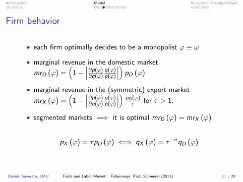
Firm behavior

• each firm optimally decides to be a monopolist ϕ ≡ ω

• marginal revenue in the domestic market

mrD (ϕ) =(

1−∣∣∣∂p(ϕ)∂q(ϕ)

q(ϕ)p(ϕ)

∣∣∣) pD (ϕ)

• marginal revenue in the (symmetric) export market

mrX (ϕ) =(

1−∣∣∣∂p(ϕ)∂q(ϕ)

q(ϕ)p(ϕ)

∣∣∣) pD(ϕ)τ for τ > 1.

• segmented markets =⇒ it is optimal mrD (ϕ) = mrX (ϕ)

pX (ϕ) = τpD (ϕ) ⇐⇒ qX (ϕ) = τ−σqD (ϕ)



Revenue

• revenue from the domestic market rD (ϕ) = YM p (ϕ)1−σ

• revenue from the export market rX (ϕ) = τ1−σrD (ϕ)

• total revenue r (ϕ) =[1 + e (ϕ) τ1−σ] rD (ϕ)

where e (ϕ) = 1 if and only if the firm exports.

inverse demand: p (ϕ)1−σ =(YM

) 1−σσ qD (ϕ)

σ−1σ

clearing: ϕl (ϕ) = qD (ϕ) + τqX (ϕ) =(1 + e (ϕ) τ1−σ) qD (ϕ)

revenue is an increasing, concave, log–linear function ofemployment

r (ϕ, l (ϕ)) =

[Y

M

(1 + e (ϕ) τ1−σ)] 1

σ

(ϕl (ϕ))σ−1σ (1)



Search and matching frictions

• there are u unemployed workers and v vacancies,define θ = v

u the labor market tightness

• the probability that a firm matches with a worker is decreasingin l.m.t. m (θ) , m′ < 0

• the probability that a worker matches with a firm is θm (θ)increasing in l.m.t.

• holding a vacancy has a cost c > 0



Law of motion for employment

• firms and workers separate with probability s = δ + χ− δχ,that is because of:

– a firm destruction shock that occurs with probability δ

– a job destruction shock that occurs with probability χ

the next period employment l ′ for a for a firm that employs lworkers and holds ϑ vacancies is∗:

l ′ = (1− χ) l + m (θ)ϑ (2)

∗assuming a continuous measure of employees and vacancies.



Firm inter–temporal problem

define the firm profit:

π (ϕ, l) = r (ϕ, l)− w (ϕ, l) l − cϑ (ϕ, l)− fD − e (ϕ) fx

Firms are risk neutral, so they choose the number of vacancies thatmaximizes the expected discounted lifetime flow of profit:

Π (ϕ, l) = maxϑ>0

1

1 + r

π (ϕ, l) + (1− δ) Π

(ϕ, l ′

)(3)

subject to:the revenue (1)the law of motion for employment (2).



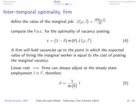
Inter–temporal optimality, firm

define the value of the marginal job: J (ϕ, l) = ∂Π(ϕ,l)∂l

compute the f.o.c. for the optimality of vacancy posting:

c = (1− δ) m (θ) J(ϕ, l ′

)(4)

A firm will hold vacancies up to the point in which the expectedvalue of hiring the marginal worker is equal to the cost of postingthe marginal vacancy.

Linear cost =⇒ firms can always adjust at the steady stateemployment l ≡ l ′, therefore:

ϑ =χ

m (θ)l (5)



Inter–temporal optimality, firm

Solve for the value of a job from the inter–temporal problem (3),

when posting is optimal c = (1− δ) m (θ) J (ϕ, l ′)

(1 + r) J (ϕ, l) =∂r

∂l− ∂w

∂ll − w − c

∂ϑ

∂l+

c

m (θ)

∂l ′

∂l

where vacancies are optimally chosen ϑ = χm(θ) l such that

employment is in steady state l ′ = l

J (ϕ, l) =1

1 + r

[∂r

∂l− ∂w

∂ll − w +

(1− χ) c

m (θ)

](6)



Inter–temporal optimality, worker

Worker are risk neutral, so they search for a job to maximize theexpected discounted lifetime flow of income:

• value of being employed (and working)

rE (ϕ, l) = w (ϕ, l) + s[U − E

(ϕ, l ′

)]• value of being unemployed (and searching)

rU = bw + θm (θ)[E(ϕ, l ′

)− U

]• steady state l ≡ l ′

E (ϕ, l)− U =w (ϕ, l)− rU

r + s(7)



Wage determination

within the period,

the wage is the outcome of a Nash bargaining,

in which the firm bargains with every worker on how to split thesurplus of the marginal job:

βJ (ϕ, l) = (1− β) [E (ϕ, l)− U]

which together with the worker’s surplus (7) yields

(r + s) J (ϕ, l) =1− ββ

(w (ϕ, l)− rU) (8)



Wage equation

The system of value of a job (6) and optimality in vacancy posting(4) yields the job creation condition,

(r + s) J (ϕ, l) =

[∂r (ϕ, l)

∂l− ∂w (ϕ, l)

∂ll − w (ϕ, l)

](9)

which in conjunction with the bargaining equation (8) yields thewage equation:

w (ϕ, l) = β

(∂r (ϕ, l)

∂l− ∂w (ϕ, l)

∂ll

)+ (1− β) rU (10)



One wage!The wage equation (10) is an O.D.E. in w (l) with a particular

solution w = (1− β) rU + β(

σσ−β

)∂r∂l , which I refer to as (?).

Solving for the revenue (1), allows to compute the monopsony

component of wages ∂w∂l l = − 1

σ

[β(

σσ−β

)∂r∂l

]< 0.

Inserting this result in the job creation condition (9), where

J (ϕ, l) = c(1−δ)m(θ) yields w =

(σ

σ−β

)∂r∂l −

(r+s1−δ

)c

m(θ) , which I

refer to as (??).

The system with the solution of the wage equation (?) yields:

w (ϕ, l) = rU +

(β

1− β

)(r + s

1− δ

)c

m (θ)∀ ϕ, l (11)



The Wage curve

Since there is one wage, w ≡ w , which allows to solve for theoutside option of the unemployed rU = bw + β

1−βcθ

1−δ .Inserting this result in the (11) yields the first equilibrium conditionthe Wage Curve:

w =β

1− βc

(1− b) (1− δ)

[r + s

m (θ)+ θ

](12)

The wage curve describes an increasing and convex relationshipbetween wage and labor market tightness.



The Labor Demand curve

Look at (??), and use the definition of marginal revenue tosubstitute for ∂r

∂l =(σ−1σ

)p (ϕ)ϕ.

As in Melitz (2003) define ϕ the productivity of the firm withaverage revenue. Then p (ϕ) coincides with the C.E.S.consumption based price index of the aggregate good, which is thenumeraire, so p (ϕ) = 1.

This allows to write the wage (??) as

w =

(σ

σ − β

)ϕ−

(r + s

1− δ

)c

m (θ)(13)

an increasing function of the measure of average productivity ϕ,and a decreasing function of labor market tightness θ.



Equilibrium



The effect of trade on the average wage

Notice that from now on the solution of the model follows Melitz(2003).

A trade liberalization, τ ↓ or fX ↓, that determines an increase inthe average productivity will lead to:

• higher wage w ↑, both in nominal and in real terms.

• higher labor market tightness θ ↑



The effect of trade on unemployment

The job finding probability is increasing in labor market tightnessθm (θ) ↑

The steady state unemployment rate has to satisfy the Beveridgecurve. Let 1− u be the number of workers unemployed, thens (1− u) = θm (θ) u implies:

u =s

s + θm (θ)(14)

A trade liberalization, τ ↓ or fX ↓, that determines an increase inthe average productivity leads to a lower unemployment.


Date post:	19-Mar-2022
Category:	Documents
Upload:	others
View:	1 times
Download:	0 times

Trade and Labor Market: Felbermayr, Prat, Schmerer (2011)

Documents