Trade and the Location of Two Industries: A Two-Factor Model

Yiming ZHOU1, Chutokuro IMAIZUMI2, Tatsuhito KONO2, and Dao-Zhi ZENG2;�

1Jiangxi University of Finance and Economics, Nanchang 330-013, China2Graduate School of Information Sciences, Tohoku University, Sendai 980-8579, Japan

We study a two-country two-factor model with free entry and monopolistic competition. There are twoindustries employing immobile labor as fixed input and mobile capital as marginal input. Firms cannot moveacross countries, but only move across industries within a country. The two industries can differ in three aspects:factor intensities, transport costs and demand elasticities. The two countries are identical except for size. Theproduction specialization and trade pattern are the results of the interaction of two effects: the market access effectand the wage differential effect.

KEYWORDS: market access effect, production specialization, trade pattern, wage differential effect

1. Introduction

The last few decades have witnessed a remarkably large reduction of trade costs and a closer economic integration.The European Union (EU) is unquestionably the most integrated regional trade agreement (RTA) in the world.Although member countries hope that deep integration will accelerate their economies, the impacts of trade integrationon various industries are still controversial.

The effects of country size differences have been a focus of attention for many years in the literature of new tradetheory (NTT) (e.g. Markusen, 1981; Markusen and Melvin, 1981; Krugman, 1980; Helpman and Krugman, 1985) andnew economic geography (NEG) (e.g. Krugman, 1991; Krugman and Venables, 1995). The most famous result in thisarea is the home market effect (HME) of Krugman (1980) and Helpman and Krugman (1985). They study a worldeconomy producing differentiated varieties subject to internal increasing returns to scale. When the differentiatedproducts are costly to trade, firms concentrate in large countries in order to save transport costs.

Some subsequent studies have tried to assess the robustness of the home market effect and to analyze the influence ofthis effect on economic distribution and trade pattern by using alternative assumptions. For example, Davis (1998)investigates whether the result of home market effect depends on the assumption of zero transport costs for thehomogeneous good. He shows that in a focal case in which differentiated and homogeneous goods have identicaltransport costs, the home market effect disappears. Moreover, several studies examine the economic location issue byincorporating a more realistic agricultural sector. For instance, keeping the usual immobile labor sector, Takatsuka andZeng (2012a, 2012b) build a general equilibrium model with general agricultural transport costs. Takatsuka and Zeng(2012a) show the exact threshold value of the agricultural transport cost for the HME in terms of firm share to occur. Incontrast, Takatsuka and Zeng (2012b) demonstrate that the HME always exists for any agricultural transport costs byincluding mobile capital as the second production factor.

Another notable study of Takahashi et al. (2013) successfully revisits the home market effect by removing thehomogeneous good in the footloose capital model. They show that the larger country has a higher wage rate and thewage differential evolves in a bell shape in terms of transport costs.

This article aims to study how the size of a country matters in determining its production specialization and tradepattern with multiple industries. Specifically, we try to answer the following questions: how does a difference in sizebetween two countries affect the equilibrium wages of these countries? What is the impact of transport costs on thewage differential? How does a continuous fall in transport costs affect the production specialization and trade pattern?

Some of these issues are firstly addressed in Amiti (1998). Amiti studies the relation between country size and inter-industry trade in a general equilibrium model with two countries, two imperfectly competitive industries. The twocountries are identical except for size. Transport costs affect both industries. The production specialization and tradepattern are results of interplay of two effects: the ‘‘market access’’ effect and ‘‘production cost’’ effect. The latter attracts

JEL Classification: F02; F12; F15; F17.

The first author is grateful to the scholarship provided by China Scholarship Council for his doctoral study at Tohoku University. All authors thank

two anonymous referees for valuable comments and suggestions that have greatly improved the paper. This research was partially funded by JSPS

KAKENHI Grant Numbers 26380282, 24243036, 24330072 of Japan.�Corresponding author. E-mail: zeng@se.is.tohoku.ac.jp

Received November 9, 2014; Accepted October 14, 2015; J-STAGE Advance published November 13, 2015

Interdisciplinary Information Sciences Vol. 22, No. 1 (2016) 1–15#Graduate School of Information Sciences, Tohoku UniversityISSN 1340-9050 print/1347-6157 onlineDOI 10.4036/iis.2015.R.02

firms to the smaller country due to lower wages. The prices in the smaller country are lower than in the larger country ineach industries.

Another study of Laussel and Paul (2007) investigate the issues by a two country and one factor model. The onlyfactor is labor which can freely move across industries but cannot move internationally. They show that if the twocountries are sufficiently close in size and demand elasticities differ across industries, a continuous fall in transportcosts is associated with a reversal in the pattern of trade at some intermediate level. On the other hand, if the twocountries are very different in size and demand elasticities differ across industries, the larger country is always a netexporter of the less differentiated good.

Chen and Zeng (2014) demonstrate an evolution of spatial sorting of high- and low-quality firms in a generalequilibrium model with segmented preferences and firm heterogeneity in demand elasticity. They show that in tworegions with identical population sizes, high-quality firms agglomerate in the region that accommodates more high-skilled labor, whereas low-quality firms move to the region that hosts more low-skilled labor in response to tradeliberalization.

Since Martin and Rogers (1995), most existing footloose capital models assume that capital is the fixed input andlabor is the marginal input in the manufacturing production. A merit of this setup is that firms’ relocation can bedescribed by the mobile capital. In a recent paper of Peng and Zeng (2014), their roles are exchanged to analyze theimpact of globalization on an economy without industrial relocation. Their model turns out to be more tractable. Wenow apply their idea to investigate the location of two industries for three reasons. First, although the total number offirms in a country becomes constant because of the labor immobility across countries, the firms can relocate acrossindustries. This model is expected to provide more detailed information of industrial relocation in the domestic market.Second, this approach can examine the robustness of the results based on the existing models. Third, in somemanufacturing industries (e.g. the design and processing industry of platinum, gold, and silver jewelry), workers withintellectual property or know-how are employed as fixed input while capital taking the form of raw materials is used asmarginal input.

As in Amiti (1998) and Laussel and Paul (2007), there are two kinds of driving forces in this article. The first one isthe market access effect which attracts firms to locate in the larger country to save on transport costs. The second one is‘‘wage differential effect’’ first called in Laussel and Paul (2007), which is similar to the ‘‘production cost effect’’ ofAmiti (1998). In our paper, this effect is quite different from theirs. The immobile labor is chosen as marginal input inboth of these two papers, therefore, the prices are lower in the smaller country in each industry. By contrast, mobilecapital is chosen as the only marginal input thus the prices equal across countries in each industry in this paper. Thewage differential effect in this article arises only from the different fixed costs. We seek to contribute to the literature byshowing that if prices equal across countries in each industry, some new results can be generated.

The wage differential evolves in a bell shape regarding transport costs both in Amiti (1998) and in this article.However, this property is totally tractable in our model when two industries only differ in factor intensities. While theresults in Amiti (1998) are restricted in interior equilibrium, we extend it to the corner equilibrium. We show the homemarket effect in terms of wages not only in interior equilibrium but also in corner equilibrium. When two industriesonly differ in demand elasticity, Amiti (1998) shows that the smaller country is more specialized in the production oflow-elasticity goods and hence a net exporter of low-elasticity goods at transport cost level close to autarky. In contrast,when transport cost level is close to autarky, the market access effect dominates in this article. Thus, the larger countryis more specialized in the production of low-elasticity goods at transport cost level close to autarky. Our results of tradepattern show that the larger country is a net exporter of both industry goods when trade is close to autarky. The netexport of high-elasticity goods increases and that of low-elasticity goods decreases when trade is close to free. Ourresults of trade pattern contrast with Laussel and Paul (2007), who employ a one-factor model. The result of tradepattern in Laussel and Paul (2007) depends on the differential of country size. Since the immobile labor is the onlyfactor in Laussel and Paul (2007), if the two countries are very different in size, most of the firms are located in thelarger country. Thus, the larger country is always a net exporter of the low-elasticity goods.

When two industries only differ in transport costs, Amiti (1998) shows that the smaller country is always morespecialized in the production of low transport cost goods and hence a net exporter of low transport cost goods. Incontrast, in this article our results show that when transport costs are close to autarky level, the larger country is morespecialized in the production of low transport cost goods. The results of trade pattern are similar to the case that twoindustries differ only in terms of demand elasticity.

The rest of the paper is constructed as follows. Section 2 sets up the model. Section 3 studies the equilibrium of themodel. Section 4 accesses the wage differential effect. Section 5 analyzes the pattern of trade and productionspecialization. Finally, Section 6 makes some concluding comments.

2. The Model

There are two manufacturing industries which employ labor, L, and capital, K. To rule out the H-O comparativeadvantage, each consumer is assumed to hold one unit of capital, so K ¼ L. Capital is perfectly mobile between thecountries whereas labor can only move within a country. The two imperfectly competitive industries are labeled by

2 ZHOU et al.

subscripts k ¼ 1; 2. The market structure is one of Chamberlinian monopolistic competition. There are many firms inboth industries, each employing increasing returns to scale technology and producing differentiated goods. Thetwo industries can differ in three respects: relative factor intensities, level of transport costs and elasticity of demand.The population share in Home, �, is assumed to be larger than 1/2. We denote variables pertaining to Foreign by anasterisk (�).

2.1 Consumers

Consumers in both countries have a Cobb-Douglas preference, given by U ¼ C0:51 C0:5

2 , where

Ck ¼Xnki

c�k�1�k

ki þXn�kj

mkj

�k

� ��k�1�k

24

35

�k�k�1

ð2:1Þ

is the aggregate consumption of industry k goods produced in both countries. To focus on the impact of country size onproduction specialization and trade pattern, we keep other aspects of these two industries as symmetric as possible.Thus, consumers here have a preference with the same expenditure share on each industry goods. This assumption alsohelps to simplify mathematical expressions. In Eq. (2.1), �k > 1 is the elasticity of substitution between any pair ofdifferentiated goods in industry k, nk is the number of industry k goods produced in the home country, cki isconsumption in the home country of industry k good i produced in the home country, and mkj is the amount of good j

in industry k shipped from the foreign to the home country.Let � ¼ �2 � �1��2

2 be the trade freeness of industry 2, and we assume �1 ¼ ��2 with � � 1. The trade freeness of

industry 1 then becomes �1 ¼ ��ð�1�1Þ�2�1 . If � ¼ 1, two industries have identical transport costs; if � > 1, transport costs

of industry 1 goods are higher than that of industry 2 goods.The price index is given as

Pk ¼Xnki

p1��kki þ

Xn�kj

ðp�kjÞ1��k�k

" # 11��k

; ð2:2Þ

where pki is the producer price set by firm i industry k in the home country and p�ki is the producer price set by firm j

in industry k in the foreign country. Maximization of the utility function subject to the budget constraint allocatesexpenditure between the two industries as follows:

P1C1 ¼1

2Y ; P2C2 ¼

1

2Y : ð2:3Þ

The consumer maximizes the sub-utility function subject to the budget constraint to derive demand functions for eachindustry 1 good produced in the home country and in the foreign country:

c1i ¼1

2p��1

1i P�1�11 Y ; m1j ¼

1

2�1��1

1 p�1j��1P�1�1

1 Y: ð2:4Þ

The demand functions for industry 2 goods are derived in the same way.

2.2 Firms

Borrowing the technology from Peng and Zeng (2014), production for any variety of each firm requires �k units ofimmobile labor as the fixed input and mobile capital as marginal input. We choose unit of products so that one unit ofmobile capital is required to produce one unit of each variety as the marginal input. And it is clear that capital can beemployed in two countries. Due to the free mobility of capital, the capital returns in two countries are equalized atequilibrium. We take this capital return as numeraire. As argued in Peng and Zeng (2014), this production technologydescribes the situation that labor is used to ‘‘design the production line’’ (Peng et al., 2006) that captures the diversity ofdifferential products, while capital is used to produce each unit of the product, whose amount is dependent on thequantity of firms’ output. For example, in the design and processing industry of platinum, gold, and silver jewelery,workers with highly trained skills and know-how are employed as fixed input while capital takes the form of rawmaterials and is used as marginal input. We assume Samuelson’s iceberg international transportation costs: � (� 1)units of a manufactured good must be shipped for one unit of requirement in the other country. The production of eachvariety is split into domestic and foreign markets. A firm in industry k producing variety i in Home sets prices of goodsto maximize its profit as

�ki ¼ pkiXki � ð�kwþ XkiÞ; ð2:5Þ

where w is the nominal wage rate of each worker in Home.Firms maximize profits with respect to quantity gives the optimal price as:

Trade and the Location of Two Industries 3

pki ¼�k

�k � 1: ð2:6Þ

Imposing the free entry and exit condition, by setting profits equal to zero, determines the quantity of output required tocover fixed cost:

Xki ¼ ð�k � 1Þw�k: ð2:7Þ

The firms are assumed to be symmetric, so Eq. (2.7) does not depend on the firm name. Notations cki, mkj, pki, and p�kjare simplified as ck, mk, pk, and p�k , respectively.

3. Equilibrium of the Model

In this section, we solve the equilibrium of the model and obtain the equations of equilibrium distribution of firmswhich will be used later for studying the production specialization and trade pattern.

3.1 Equilibrium of the factor market

We turn to the factor market equilibrium conditions. First of all, the labor market equilibrium condition is

n1�1 þ n2�2 ¼ L�; n�1�1 þ n�2�2 ¼ Lð1� �Þ: ð3:1Þ

The left hand sides of the equations are total labor employment and the right hand sides are total labor supply for eachcountry. On the other hand, the capital market equilibrium condition is

ð�1 � 1Þ�1ðn1wþ n�1w�Þ þ ð�2 � 1Þ�2ðn2wþ n�2w

�Þ ¼ L: ð3:2Þ

3.2 The equilibrium distribution of firms

We need the product market equilibrium to close the model. If Home (resp. Foreign) accommodates some firms ofindustry k ¼ 1; 2, then

Xk ¼ ck þ m�k ; ðresp. X�k ¼ c�k þ mkÞ ð3:3Þ

holds. The price indexes are

Pk ¼�k

�k � 1ðnk þ n�k�kÞ

11��k ; P�k ¼

�k

�k � 1ðnk�k þ n�kÞ

11��k ; ð3:4Þ

where �k ¼ �1��kk . Each country is endowed with equal capital to labor ratios, hence

Y ¼ L�ðwþ rÞ; Y� ¼ Lð1� �Þðw� þ r�Þ; ð3:5Þ

where r and r� are the capital prices in two countries, which are equal by the perfect mobility assumption.Plugging Eqs. (2.2), (2.4), (2.7), (3.4), and (3.5) into (3.3), we obtain the following four equations

L�ðwþ 1Þnk þ n�k�k

þLð1� �Þ w� þ 1ð Þ�k

�knk þ n�k¼ 2�kw�k; k ¼ 1; 2 ð3:6Þ

L�ðwþ 1Þ�knk þ n�k�k

þLð1� �Þ w� þ 1ð Þ

�knk þ n�k¼ 2�kw

��k; k ¼ 1; 2 ð3:7Þ

in an interior equilibrium. By multiplying (3.6) by nk, (3.7) by n�k and adding them up, we obtain

�1�1ðn1wþ n�1w�Þ ¼ �2�2ðn2wþ n�2w

�Þ:By use of (3.2), we thus have

n1wþ n�1w� ¼

L�2

�1ð2�1�2 � �1 � �2Þ; ð3:8Þ

n2wþ n�2w� ¼

L�1

�2ð2�1�2 � �1 � �2Þ; ð3:9Þ

�wþ ð1� �Þw� ¼�1 þ �2

2�1�2 � �1 � �2

: ð3:10Þ

Equation (3.10) is the average labor income. Adding the capital returns, we obtain the total average income as

1þ �wþ ð1� �Þw� ¼2�1�2

2�1�2 � �1 � �2

:

Since labor is the fixed input of production, its share in the total production is

4 ZHOU et al.

�1 þ �2

2�1�2

¼1

2

1

�1

þ1

�2

� �:

It is well known that the share of the fixed input is 1=� in the case of a single industry. Interestingly, we find the similarproperty in which the share becomes the average of two industries.

Meanwhile, since the RHS of (3.10) is constant, this equation shows that w is negatively related to w�. Namely, wincreases if and only if w� decreases.

Equations (3.1), (3.2), (3.8), (3.9) and (3.10) provide simple expressions for variables n�1, n2, n�2, w� in terms of n1

and w:

n�1 ¼L�2 � ð2�1�2 � �1 � �2Þn1w�1

�1 þ �2 � ð2�1�2 � �1 � �2Þ�w1� ��1

; ð3:11Þ

n2 ¼�L� �1n1

�2; ð3:12Þ

n�2 ¼Lð1� �Þ � �1n�1

�2¼ð1� �ÞL�2

�L�2 � ð2�1�2 � �1 � �2Þn1w�1

�1 þ �2 � ð2�1�2 � �1 � �2Þ�w1� ��2

; ð3:13Þ

w� ¼�1 þ �2

ð2�1�2 � �1 � �2Þð1� �Þ�

�

1� �w: ð3:14Þ

Note that n1 and w can be obtained from Eqs. (3.6) and (3.7) for two different industries.Equation (3.12) and the first equality of (3.13) show that the pair of n1 and n2 and the pair of n�1 and n�2 are negatively

related.Finally, in an interior equilibrium, taking the ratio of the equilibrium product market conditions for industry k in

Foreign to Home derives

�ðwþ 1Þ�nk

n�k�k þ 1

�þ �kð1� �Þðw� þ 1Þ

�nk

n�kþ �k

�

�k�ðwþ 1Þ�nk

n�k�k þ 1

�þ ð1� �Þðw� þ 1Þ

�nk

n�kþ �k

� ¼ w

w�: ð3:15Þ

3.3 Autarky and free trade

In the case of autarky, we have �k ¼ 0. Equation (3.6) degenerates to L�ð1þwÞ=nk ¼ 2�k�kw for k ¼ 1; 2. By use of(3.12), we can solve out n1 and w. Meanwhile, Eqs. (3.7), (3.11)–(3.14) can be used to solve all other variables. Thesolution is

w ¼ w� ¼�1 þ �2

2�1�2 � �1 � �2

; ð3:16Þ

n1 ¼L��2

�1 �1 þ �2ð Þ; n2 ¼

L��1

�2 �1 þ �2ð Þ; n�1 ¼

Lð1� �Þ�2

�1 �1 þ �2ð Þ; n�2 ¼

Lð1� �Þ�1

�2 �1 þ �2ð Þ: ð3:17Þ

The results of (3.17) reveal that n1=n2 ¼ n�1=n�2. Therefore, the larger country is just a scale expansion of the smaller

country in the case of autarky. In fact, since there is no trade, the demand and supply of each industry in each countryare balanced. On the other hand, each firms in each industry produces the same amount of output in equilibrium.

To show how wages and firm location change at � ¼ 0, we calculate the derivatives of these important variables asfollows.

@w

@�

�����¼0

¼2ð2� � 1Þ�2

1�2

�ð2�1�2 � �1 � �2Þ2> 0; ð3:18Þ

@w�

@�

�����¼0

¼ �2ð2� � 1Þ�2

1�2

ð1� �Þð2�1�2 � �1 � �2Þ2< 0; ð3:19Þ

@n1

@�

�����¼0

¼ �Lð2� � 1Þ�1�2

�1 �1 þ �2ð Þ2< 0;

@n2

@�

�����¼0

¼Lð2� � 1Þ�1�2

�2 �1 þ �2ð Þ2> 0; ð3:20Þ

@n�1@�

�����¼0

¼Lð2� � 1Þ�1�2

�1 �1 þ �2ð Þ2> 0;

@n�2@�

�����¼0

¼ �Lð2� � 1Þ�1�2

�2 �1 þ �2ð Þ2< 0: ð3:21Þ

Therefore, w, n2 and n�1 increase while w�, n1 and n�2 decrease at � ¼ 0.While we have only an interior equilibrium at � ¼ 0, the equilibrium at �k ¼ 1 can be either interior or corner. If

�1 ¼ �2, the equilibrium at � ¼ 1 is interior and we have

Trade and the Location of Two Industries 5

w ¼ w� ¼1

� � 1; n1 ¼

L�

2�1; n2 ¼

L�

2�2; n�1 ¼

Lð1� �Þ2�1

; n�2 ¼Lð1� �Þ

2�2:

On the other hand, if �1 > �2, there exists a threshold value of �] 2 ð0; 1Þ, such that a corner equilibrium with n�1 ¼ 0

occurs when � 2 ½�]; 1�. Such a corner equilibrium is solved in Appendix A and its uniqueness is examined inAppendix B. At � ¼ 1, the wages are given by (3.16) again while the industrial location at the corner equilibrium isgiven by

n1 ¼L�2

�1 �1 þ �2ð Þ; n�1 ¼ 0; n2 ¼

L

�2

�1� � �2ð1� �Þ�1 þ �2

� �; n�2 ¼

Lð1� �Þ�2

:

Furthermore, to show the dependence of those variable when � approaches 1, we have the following results ofderivatives.

@w

@�

�����¼1

¼ �L2ð1� �Þð2� � 1Þ�2

2

�2ð�1 þ �2Þð2�1�2 � �2 � �1Þn21

< 0;

@w�

@�

�����¼1

¼L2�ð2� � 1Þ�2

2

�2 �1 þ �2ð Þ 2�1�2 � �2 � �1ð Þn21

> 0;

@n1

@�

�����¼1

¼Lð1� �Þð2� � 1Þ�2

�ð�1 þ �2Þ> 0;

@n2

@�

�����¼1

¼ �Lð1� �Þð2� � 1Þ�2

�ð�1 þ �2Þ< 0:

Therefore, the wages in Home decrease and the wages in Foreign increase to the same level of (3.16). Regarding thefirm location, industry 1 agglomerates in Home and expands while industry 2 shrinks and moves to Foreign for� 2 ½�]; 1�.

4. The Wage Differential

There are two kinds of driving forces in this model: the market access effect and the wage differential effect. Theinteraction between these two effects determines the production specialization and the direction of trade. In this section,we examine the wage differential.

Proposition 4.1. For both interior equilibrium and corner equilibrium, we have w > w� for 0 < � < 1.

Proof: Firstly, we show that w=w� 6¼ 1 for 0 < � < 1 at the interior equilibrium. To the contrary, assume thatw ¼ w� for some � 2 ð0; 1Þ. Equation (3.15) becomes:

�ðnkn�k

�k þ 1Þ þ �kð1� �Þðnkn�k

þ �kÞ

�k�ðnkn�k

�k þ 1Þ þ ð1� �Þðnkn�k

þ �kÞ¼ 1;

implying

nk

n�k¼� � �kð1� �Þ1� �ð1þ �kÞ

>�

1� �; k ¼ 1; 2:

The above inequalities n1=n�1 > �=ð1� �Þ and n2=n

�2 > �=ð1� �Þ violate (3.1).

Next, by use of (3.18) and (3.19) we have

@

@�

w

w�

�����¼0

¼2ð2� � 1Þ�2

1�2

ð1� �Þ�ð�1 þ �2Þð2�1�2 � �2 � �1Þ> 0:

Given the same wage level of (3.16) at � ¼ 0, we know that w > w� for � 2 ð0; 1Þ as long as the equilibrium is interior.Finally, Appendix A shows that w > w� also holds at the only possible corner equilibrium with n�1 ¼ 0. Therefore,

the positive wage differential of w > w� occurs at any � 2 ð0; 1Þ, no matter whether the equilibrium is interior orcorner. �

The above result is called the home market effect in terms of wages (Takahashi et al. 2013), which is firstly obtainedby Krugman (1980) for the case of a single industry, saying that ‘‘the larger country, other things being equal, will havethe higher wage.’’ Amiti (1998) and Laussel and Paul (2007) also have the home market effect in terms of wages. Whilethis effect in Amiti (1998) are restricted in interior equilibrium, we extend it to the corner equilibrium. On the otherhand, unlike Amiti (1998) and this article, Laussel and Paul (2007) employ a one-factor model. The relation betweenwage ratio w=w� and transport costs are monotonic. In contrast, the numerical results presented in Amiti (1998) andthis article suggest that the relation between w=w� and � is bell-shaped. In our model, this bell-shaped pattern isanalytically shown (see Lemma 5.1) when two industries differ only in terms of factor intensity.

6 ZHOU et al.

5. The Industrial Location and Trade Pattern

In this section, we focus on three differences between two industries: the relative factor intensity, the transport costsand the demand elasticity. We study how the differences affect the firm location and trade pattern when transport costsfall from a prohibitive level to zero.

As noted earlier, there are two opposite effects in our model: the market access effect and the wage differential effect.Reducing transport costs from the autarky level to some finite level makes the large market more attractive. Because thefirms in the smaller country find that the gains in exports do not offset the sales lose in the domestic market so theamount of output is insufficient to cover fixed costs and this leads to the exit of some firms. On the other hand, thedemand for factors in the larger country would increase. An increase in the demand for capital in the larger countryresults in capital flowing from the smaller country to the larger country. In contrast, an increase in the demand for laborin the larger country pushes up wages in the larger country since labor is not mobile. A lower wage rate in the smallercountry offsets the locational advantage of the larger country.

5.1 Different factor intensity

Our first case is that two industries only differ in the factor intensity of production. Namely, we have �1 ¼ �2 ¼ �,� ¼ 1 while �1 6¼ �2. The model is completely solved in this case.

Lemma 5.1. If two industries only differ in factor intensity, the wages and the firm numbers are given by

w ¼ð1� �Þ�ð� � 1Þ þ ���þ ð1� �Þ½� þ �ð1� �Þ��2

ð1� �Þ�ð� � 1Þ2 þ ½ð1� �Þ2 þ �2�ð� � 1Þ��þ ð1� �Þ�ð�2 � 1Þ�2; ð5:1Þ

w� ¼ð1� �Þ�ð� � 1Þ þ ð1� �Þ��þ �ð1� � þ ��Þ�2

ð1� �Þ�ð� � 1Þ2 þ ½ð1� �Þ2 þ �2�ð� � 1Þ��þ ð1� �Þ�ð�2 � 1Þ�2; ð5:2Þ

n1 ¼L�

2�1; n2 ¼

L�

2�2; n�1 ¼

Lð1� �Þ2�1

; n�2 ¼Lð1� �Þ

2�2: ð5:3Þ

When � increases from 0 to 1, wage rate w exhibits a bell shape while w� has a U shape.

Proof: By use of �1 ¼ �2 ¼ � and �1 ¼ �2, we have n1=n2 ¼ n�1=n�2 from Eq. (3.15). Then Eqs. (3.11), (3.12), and

(3.13) immediately imply (5.3). Furthermore, (5.1) and (5.2) can be easily derived from (3.14) and one of (3.6). Nowwe treat w of (5.1) as a function of �. Evidently, for any w], equation wð�Þ ¼ w] has at most two solutions of �.Therefore, in the �-w plane, the curve wð�Þ crosses any horizontal line w ¼ w] at most twice. Given inequality (3.18)at � ¼ 0 and equality (3.16) at both � ¼ 0 and � ¼ 1, wð�Þ has a bell shape. Since w and w� are negatively relatedaccording to (3.10), curve w�ð�Þ has a U shape. �

It is noteworthy that the above lemma also shows that wage differential w� w� and w=w� evolve as a bell-shapedcurve when trade costs fall.

The reason that two countries share the same production pattern for any transport costs is not mysterious. The fact ofequal wages at autarky means that firms in each industry have the same output. The total output share in industry k acrosscountries should be equal to the consumption share (or labor share, since preferences are identical). Therefore, therelative firm numbers in industry k across countries are equal to the consumption share: n1=n

�1 ¼ n2=n

�2 ¼ �=ð1� �Þ. On

the other hand, the consumption share between industry 1 and industry 2 goods in each country should be equal to theproduction share n1X1i=ðn2X2iÞ. It explains the result of n1=n2 ¼ �2=�1 at autarky. To explain the same ratio holds for alltrade costs, it is helpful to notice an important difference between Amiti (1998) and this article. The immobile labor ischosen as fixed input, hence firms can not move across countries but only move across industries within a country.Suppose that the transport costs fall to some finite level, firms in industry k have no incentive to move to the otherindustry if �1 ¼ �2 and �1 ¼ �2, since the price and mark-up of each industry equals when mobile capital is chosen asthe only marginal input. Therefore, even when the transport costs fall, two countries keep the same production pattern.

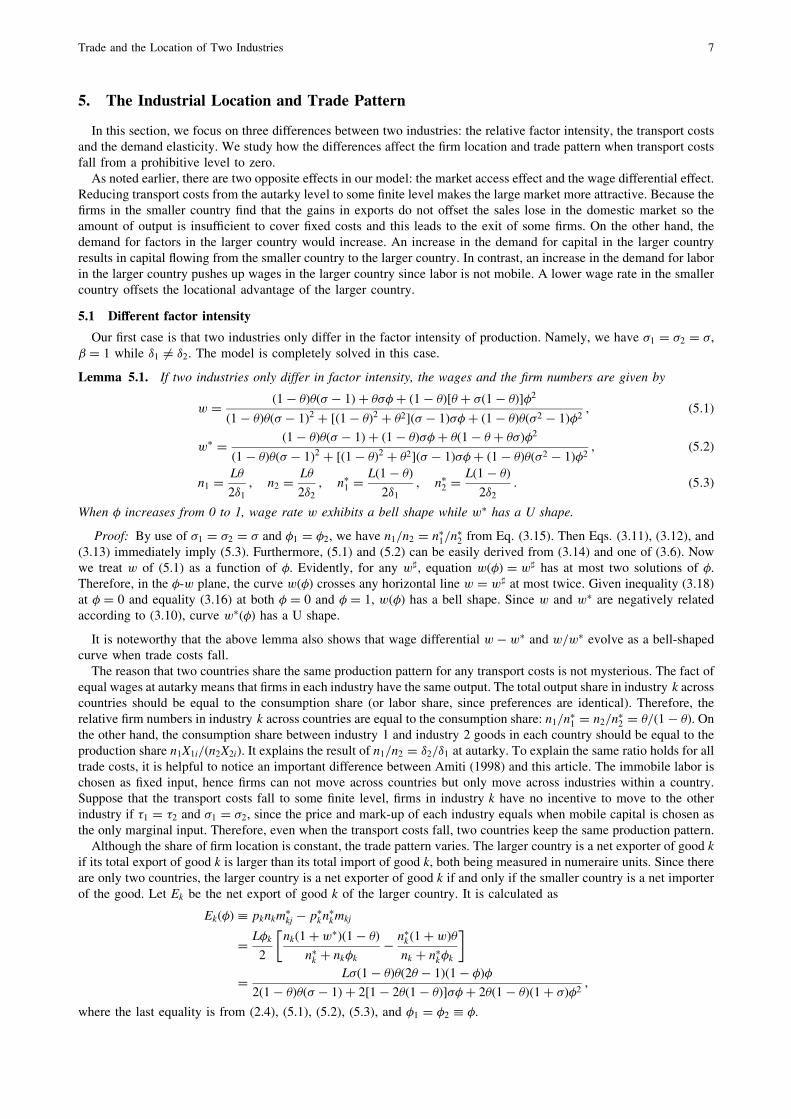
Although the share of firm location is constant, the trade pattern varies. The larger country is a net exporter of good k

if its total export of good k is larger than its total import of good k, both being measured in numeraire units. Since thereare only two countries, the larger country is a net exporter of good k if and only if the smaller country is a net importerof the good. Let Ek be the net export of good k of the larger country. It is calculated as

Ekð�Þ � pknkm�kj � p�kn

�kmkj

¼L�k

2

nkð1þ w�Þð1� �Þn�k þ nk�k

�n�k ð1þ wÞ�nk þ n�k�k

� �

¼L�ð1� �Þ�ð2� � 1Þð1� �Þ�

2ð1� �Þ�ð� � 1Þ þ 2½1� 2�ð1� �Þ���þ 2�ð1� �Þð1þ �Þ�2;

where the last equality is from (2.4), (5.1), (5.2), (5.3), and �1 ¼ �2 � �.

Trade and the Location of Two Industries 7

Curve Ekð�Þ has only one stationary point

~�1 ¼ffiffiffiffiffiffiffiffiffiffiffiffiffiffiffiffiffiffiffiffiffiffiffiffiffiffiffiffiffiffiffið1� �Þ�ð� � 1Þpffiffiffi�pþ

ffiffiffiffiffiffiffiffiffiffiffiffiffiffiffiffiffiffiffiffiffiffiffiffiffiffiffiffiffiffiffið1� �Þ�ð� � 1Þp 2 ½0; 1�:

Furthermore, we have

E0kð0Þ ¼ð2� � 1ÞL�2ð� � 1Þ

> 0; E0kð1Þ ¼ ��ð1� �Þð2� � 1ÞL

2< 0:

Therefore, Ekð�Þ increases in � in ½0; ~�1Þ and decreases in � in ð ~�1; 1�.Summarizing the above discussion, we obtain the following conclusion regarding the industrial location and trade

patterns when trade costs fall.

Proposition 5.2. (i) If two industries differ only in factor intensity of production, the firm number of each industry ineach country is independent of trade costs. (ii) The wage rate in the larger country is higher and the wage differentialevolves in a bell shape. (iii) The larger country is a net exporter of both industry goods. The volume of net export alsohas a bell shape.

Note that the capital endowment of each resident in either country is the same. The capital is mobile. Since the largercountry is a net exporter in both industries, the trade balance condition implies that capital flows from the smallercountry to the larger one.

Corollary 5.3. For � 2 ð0; 1Þ, the larger country is a net importer of capital.

5.2 Different demand elasticity

In our second case, two industries are identical in all respects except the demand elasticity. Namely, �1 ¼ �2 ¼ �,� ¼ 1, �1 > �2. We first provides a result for the industry location.

Lemma 5.4. When two industries differ only in demand elasticity, there exists a ~�2 2 ð0; 1Þ at which n1=n2 ¼ n�1=n�2.

If trade is close to autarky, we have inequality n1=n2 < n�1=n�2; if trade is close to free, we have inequality

n1=n2 > n�1=n�2.

Proof: Firm numbers n1 and n�1 are non-negative. According to Appendix A, there exists a threshold value of �],such that n�1 ¼ 0 for all � � �]. The detail of this corner equilibrium is solved in Appendix A, and the uniqueness isconsidered in Appendix B. Note that n1=n2 � n�1=n

�2 ¼ 0 holds at � ¼ 0. By use of Eqs. (3.17), (3.20) and (3.21), the

differentiation of n1=n2 � n�1=n�2 with respect to � at � ¼ 0 is

@

@�

n1

n2

�n�1n�2

� ������¼0

¼ �ð2� � 1Þ�2

ð1� �Þ��1

< 0: ð5:4Þ

Therefore, n1=n2 � n�1=n�2 < 0 holds when � is close to zero. Since n1=n2 > 0 ¼ n�1=n

�2 at �], there exists a ~�2 2

ð0; �]Þ � ð0; 1Þ at which n1=n2 � n�1=n�2 ¼ 0. �

Figure 1 provides a simulation result, in which parameters are given as � ¼ 0:6, �1 ¼ 3, �2 ¼ 1:5, � ¼ 1. In the rightpanel, we can see that n1=n2 < n�1=n

�2 holds for � 2 ð0; ~�2Þ and n1=n2 > n�1=n

�2 holds for � 2 ð ~�2; 1�. Namely, the larger

country is relatively more specialized in the production of low-elasticity goods when transport costs are high and isrelatively more specialized in the production of the high-elasticity goods when trade costs are low.

Now, we analyze the trade pattern. Unfortunately, we have no explicit form for the wages and firm numbers in thiscase. However, the derivatives of Ekð�Þ at � ¼ 0 and � ¼ 1 can be calculated as

E01ð�Þj�!0 ¼L�1�2�

�1��2

�2�1

ð�1 þ �2 � 2�1�2Þ2ð2� � 1Þð�1 � 1Þð2�1�2 � �1 � �2Þ

�2 � 1þ oð�Þ

� �> 0;

E01ð1Þ ¼L�ð1� �Þð2� � 1Þ �1 þ �2ð Þ

2 2�1�2 � �2 � �1ð Þ> 0;

E02ð0Þ ¼L�1�2

2�1�2 � �1 � �2

> 0;

E02ð1Þ ¼ �L�ð1� �Þð2� � 1Þ �1 þ �2ð Þ 2�2 � 1ð Þ

2 2�1�2 � �2 � �1ð Þ< 0;

where oð�Þ is the Landau symbol ‘‘small’’ o. Therefore, Ekð�Þ is positive when � is close to autarky level. On the otherhand, E1ð�Þ increases while E2ð�Þ decreases when � is close to free trade level. We perform simulations to show someproperties of the net export of the larger country. In Fig. 2 the solid line depicts the net export of high-elasticity goodswhile the dotted line depicts the net export of low-elasticity goods. Figure 2 illustrates that the larger country is alwaysa net exporter of the high-elasticity goods. On the other hand, when transport costs are close to free trade level, the large

8 ZHOU et al.

country is a net importer of the low-elasticity goods. This result is different from that of Laussel and Paul (2007), whichemploy a one-factor model. Since the immobile labor is the only factor, the result of trade pattern in Laussel and Paul(2007) depends on the differential of country size. If the two countries are very different in size, most firms are locatedin the larger country. Thus, the larger country is always a net exporter of the low-elasticity goods. If the two countriesare sufficiently similar in size, a continuous fall in transport costs from a prohibitive level to zero is associated with areversal in the pattern of trade at some intermediate level. Finally, we examine the capital flow. Let h denote the capitalshare employed in the Home country. The ratio of home to foreign demands for capital is

h

1� h¼

n1 �1 � 1ð Þw�1 þ n2 �2 � 1ð Þw�2n�1 �1 � 1ð Þw��1 þ n�2 �2 � 1ð Þw��2

ð5:5Þ

¼ð�2 � 1ÞwL� þ n1ð�1 � �2Þw�1

ð�2 � 1Þw�Lð1� �Þ þ n�1ð�1 � �2Þw��1;

where the second equality is from Eq. (3.12) and the first equality of (3.13).According to Eq. (3.12) and the first equality of (3.13) again, we know that n1=n2 ¼ n�1=n

�2 holds only if they are

equal to �=ð1� �Þ. Therefore, n1=n2 > n�1=n�2 implies n1=n2 > �=ð1� �Þ > n�1=n

�2 so that h=ð1� hÞ > �=ð1� �Þ holds.

Thus capital employment in the larger country is more than its endowment and capital flows from the smaller country tothe larger country. Similarly, capital flows from the larger country to the smaller country when n1=n2 < n�1=n

�2.

The evolution result of industrial location when trade costs fall is summarized as follows.

Proposition 5.5. When trade is close to autarky, the larger country is relatively more specialized in the production ofthe low-elasticity goods. When trade is close to free, the larger country is relatively more specialized in the productionof the high-elasticity goods.

Intuitively, the lower is �, the higher is the mark-up over marginal cost. Suppose a decrease of price, firms in theindustry with lower demand elasticity increase sales more. Firms in both countries have incentives to enter the low-elasticity industry (a decrease of n1=n2 or n�1=n

�2). Again, there is an trade-off between the market access effect and the

wage differential effect. When transport costs are relatively high, the market access effect dominates. Firms in thelarger country succeed in entering the low elasticity industry. Thus, the specialization degree of the low elasticityindustry in the larger country increased (a decrease of n1=n2). As transport costs continue to fall, the magnitude ofmarket access effect decreases. On the other hand, the lower wages give the firms in the smaller country an advantageof entering the low elasticity industry. Now, it’s the wage differential effect dominates. Firms in the smaller countrythen succeed in increasing the specialization degree of industry 2 (a decrease of n�1=n

�2). Figure 1 illustrates that n�1=n

�2

continues to fall as transport costs approach the free trade level.This result is contrastive to Amiti (1998), which shows that the smaller country is relatively more specialized in the

n2

n1

n1

n2

0.2 0.4 0.6 0.8 1.0φ φ

1

2

3

4nk,nk

n1 n2

n1 n2

0.2 0.4 0.6 0.8 1.0

0.2

0.4

0.6

0.8

1.0

1.2

n1 n2, n1 n2

Fig. 1. nk and n�k when �1 > �2.

Industry 1

Industry 20.2 0.4 0.6 0.8 1.0

φ

2

1

1

2

3

4Net exports

Fig. 2. Net exports when �1 > �2.

Trade and the Location of Two Industries 9

production of low-elasticity goods when transport costs are close to autarky level. The reason is that the wagedifferential effect in this article and ‘‘production cost effect’’ in Amiti (1998) are quite different. A Leontief compositeof capital and labor is chosen as both fixed input and marginal input in Amiti (1998). In other words, labor wages enterboth the fixed cost and marginal cost in Amiti (1998). By contrast, the wage differential effect arises only from the fixedcosts, and prices are equal across countries in this article. On the other hand, Chen and Zeng (2014) assume labor asmarginal input and capital as fixed input. It implies that the wage differential effect in this article or Chen and Zeng(2014) is weaker than in Amiti (1998). When trade is close to autarky (market access effect is more stronger), themarket access effect dominates and the larger country has a higher degree of production specialization in the low-elasticity industry.

On the other hand, when transport costs are close to the free trade level, our result is consistent with Amiti (1998)which shows that the larger country specialize in the production of high-elasticity goods. At integration levels close tofree trade, the market access effect becomes much smaller, the wage differential effect dominates in both Amiti (1998)and this article. This result is starkly contrastive to the known home market effect in terms of firm share when theeconomy space has a single manufacturing sector and an agricultural sector. The agricultural good is homogeneous soits demand elasticity is infinitely high. Existing results of such models exhibit that the larger country accommodatesmore-than-proportionate of the manufacturing firms. Our different result can be attributed to the fact that there is nofixed costs in the agricultural production and there is no wage differential due to the assumption of free trade ofagricultural good in the existing models. If we suppose firms use capital as their fixed input and labor as their marginalinput to produce, as assumed in Chen and Zeng (2014), the low-elasticity firms show stronger agglomeration forcesthan do high-elasticity firms. Therefore, at an integration level close to free trade, low-elasticity firms, which enjoyhigher markups, agglomerate in the larger country. A comparison of results among Amiti (1998), Chen and Zeng(2014) and this article is summarized by Table 1.

5.3 Different levels of transport costs

In our third case, two industries are identical except their trade costs: �1 ¼ �2 ¼ �, �1 ¼ �2 ¼ � but �1 > �2 (i.e.,� > 1). Namely, industry 1 goods are bulkier to transport. Similar to Lemma 5.4, we have the following conclusion onindustrial location.

Lemma 5.6. There exists a ~�3 2 ð0; 1Þ at which n1=n2 ¼ n�1=n�2 holds. We have inequality n1=n2 < n�1=n

�2 when � is

close to 0, and inequality n1=n2 > n�1=n�2 when � is close to 1.

Proof: It can be proved in the same way as in Lemma 5.4. The only difference is to replace (5.4) by

@

@�

n1

n2

�n�1n�2

� ������¼0

¼ �ð2� � 1Þð1� �Þ�

< 0:

�

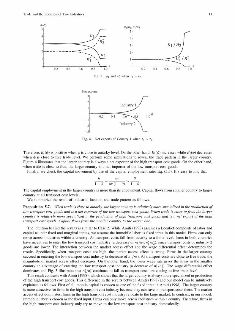
Figure 3 gives a simulation result in which parameters are given as � ¼ 0:6, � ¼ 2, � ¼ 3, � ¼ 1. We can visuallysee the threshold value ~�3, above which the larger country is relatively more specialized in the production of lowtransport cost goods.

Now, we turn to analyze the trade pattern. Unfortunately, we are unable to explicitly solve the wages and firmnumbers in this case. However, the derivatives of Ekð�Þ at � ¼ 0 and � ¼ 1 can be calculated as

E01ð�Þj�!0 ¼L���1

4ð� � 1Þ2½2�ð2� � 1Þð� � 1Þ� þ oð�Þ� > 0;

E01ð1Þ ¼L�ð1� �Þð2� � 1Þ

2ð� � 1Þ> 0;

E02ð0Þ ¼L�

2ð� � 1Þ> 0;

E02ð1Þ ¼ �Lð1� �Þ�ð2� � 1Þð2� � 1Þ

2ð� � 1Þ< 0:

Table 1. A comparison among Amiti (1998), Chen and Zeng (2014) and this article. WDE: Wage Differential Effect,MAE: Market Access Effect.

ModelAmiti (1998) Chen and Zeng (2014) This article

Effect

Trade freeness �! 0 �! 1 �! 0 �! 1 �! 0 �! 1

ResultWDE> WDE> WDE< WDE< WDE< WDE>

MAE MAE MAE MAE MAE MAE

10 ZHOU et al.

Therefore, Ekð�Þ is positive when � is close to autarky level. On the other hand, E1ð�Þ increases while E2ð�Þ decreaseswhen � is close to free trade level. We perform some simulations to reveal the trade pattern in the larger country.Figure 4 illustrates that the larger country is always a net exporter of the high transport cost goods. On the other hand,when trade is close to free, the larger country is a net importer of the low transport cost goods.

Finally, we check the capital movement by use of the capital employment ratio Eq. (5.5). It’s easy to find that

h

1� h¼

w�

w�ð1� �Þ>

�

1� �:

The capital employment in the larger country is more than its endowment. Capital flows from smaller country to largercountry at all transport cost levels.

We summarize the result of industrial location and trade pattern as follows.

Proposition 5.7. When trade is close to autarky, the larger country is relatively more specialized in the production oflow transport cost goods and is a net exporter of the low transport cost goods. When trade is close to free, the largercountry is relatively more specialized in the production of high transport cost goods and is a net export of the hightransport cost goods. Capital flows from the smaller country to the larger one.

The intuition behind the results is similar to Case 2. While Amiti (1998) assumes a Leontief composite of labor andcapital as their fixed and marginal inputs, we assume the immobile labor as fixed input in this model. Firms can onlymove across industries within a country. As transport costs fall from autarky to a finite level, firms in both countrieshave incentives to enter the low transport cost industry (a decrease of n1=n2, n�1=n

�2), since transport costs of industry 2

goods are lower. The interaction between the market access effect and the wage differential effect determines theresults. Specifically, when transport costs are high, the market access effect is strong. Firms in the larger countrysucceed in entering the low transport cost industry (a decrease of n1=n2). As transport costs are close to free trade, themagnitude of market access effect decreases. On the other hand, the lower wage rate gives the firms in the smallercountry an advantage of entering the low transport cost industry (a decrease of n�1=n

�2). The wage differential effect

dominates and Fig. 3 illustrates that n�1=n�2 continues to fall as transport costs are closing to free trade level.

This result contrasts with Amiti (1998), which shows that the larger country is always more specialized in productionof the high transport cost goods. This difference in the results between Amiti (1998) and our model can be intuitivelyexplained as follows. First of all, mobile capital is chosen as one of the fixed input in Amiti (1998). The larger countryis more attractive for firms in the high transport cost industry because they can save on transport costs there. The marketaccess effect dominates, firms in the high transport cost industry relocate to the large market. In contrast, in our model,immobile labor is chosen as the fixed input. Firms can only move across industries within a country. Therefore, firms inthe high transport cost industry only try to move to the low transport cost industry domestically.

n1n2

n2n1

0.2 0.4 0.6 0.8 1.0φ

1

2

3

4

5nk,nk

n1 n2

n1 n2

0.2 0.4 0.6 0.8 1.0φ

1

2

3

4

5n1 n2, n1 n2

Fig. 3. nk and n�k when �1 > �2.

Industry 1

Industry 2

0.2 0.4 0.6 0.8 1.0φ

3

2

1

1

2

3Net exports

Fig. 4. Net exports of Country 1 when �1 > �2.

Trade and the Location of Two Industries 11

Second, the wage differential effect in this article and ‘‘production cost effect’’ in Amiti (1998) are quite different. Asdiscussed in Section 5.2, wages enter both the fixed cost and marginal cost in Amiti (1998). However, the wagedifferential effect arises only from the fixed costs and prices are equal across countries in this article. In other words, thewage differential effect is weaker in this article than in Amiti (1998). Therefore, when trade is close to autarky (marketaccess effect is more stronger), the market access effect dominates and the larger country has a higher degree ofproduction specialization in the low transport cost industry.

6. Concluding Remarks

In this article, we studied how different industries locate and what are the trade patterns when countries havedifferent size. Both industries have technologies of increasing returns to scale. They may differ in factor intensity,demand elasticity, and trade costs. We have shown how the equilibrium results from the interplay of two forces, themarket access effect and the wage differential effect. We show the home market effect in terms of wages not only ininterior equilibrium but also in corner equilibrium. Unlike the existing literature, we choose mobile capital as marginalinput, thus the prices are equal between countries in this article. We seek to contribute to the literature by showing thatif prices are equal across countries in each industry, some new results can be generated.

We obtain the following conclusions. First, if two industries differ only in factor intensity, two countries share thesame production pattern (n1=n2 ¼ n�1=n

�2) for any trade costs. The wage rate in the larger country is higher and the wage

differential evolves in a bell shape when trade costs fall. The larger country is a net exporter of both industry goods.The volume of the net export also evolves in a bell shape.

Second, if two industries differ only in demand elasticity, the larger country is relatively more specialized in theproduction of low-elasticity goods when trade is close to autarky; the larger country is relatively more specialized in theproduction of high-elasticity goods when trade is close to free. Our results suggest that the larger country is a netexporter of both industry goods when trade is close to autarky. The net export of high-elasticity goods increases andthat of low-elasticity goods decreases when trade is close to free.

Third, if two industries differ only in transport costs, the larger country is relatively more specialized in theproduction of low transport cost goods and hence a net exporter of these goods when trade is close to autarky; the largercountry is relatively more specialized in the production of high transport cost goods and hence a net exporter of thesegoods when trade is close to free.

Appendix A: The Corner Equilibrium (�2 � �)

We examine a possible corner solution n�1 ¼ 0. By use of the labor market equilibrium equations, we can obtain n�2,n2, w and w� in terms of n1 as follows.

n�2 ¼Lð1� �Þ�2

; n2 ¼L�

�2� n1

�1

�2; ðA:1Þ

w ¼L�2

�1n1ð2�1�2 � �1 � �2Þ; w� ¼

�1n1ð�1 þ �2Þ � L��2

ð1� �Þ�1n1ð2�1�2 � �1 � �2Þ:

Plugging the equations above into the following market-clearing condition of industry 2

L�ð1þ wÞn2 þ n�2�

þLð1� �Þ 1þw�ð Þ�

�n2 þ n�2� 2�2w�2 ¼ 0;

we obtain An21 �Bn1 þ C ¼ 0, where

A � 2�21�2 �1 þ �2ð Þ� > 0;

B � L�1fð1� �Þ � �1 þ �2ð Þ þ 2ð1� �Þ�1�2 þ 2�22

� �2

þ 2��2 �1 þ 2�2ð Þ�þ ð1� �Þ ��1 2�2 � 1ð Þ þ �2 2�2 � �ð Þ½ �g > 0;

C � L2�2 2�2ð1� � þ ��Þð� � ��þ �Þ � ð1� �Þ 1� �2 �

��

> 0:

This quadratic function of n1 has two roots

n1 ¼ n1a �B�

ffiffiffiffiffiffiffiffiffiffiffiffiffiffiffiffiffiffiffiffiffiffiB2 � 4ACp

2A> 0 and n1 ¼ n1b �

BþffiffiffiffiffiffiffiffiffiffiffiffiffiffiffiffiffiffiffiffiffiffiB2 � 4ACp

2A> 0:

They correspond to two values of n2

n2a �2AL� �B�1 þ �1

ffiffiffiffiffiffiffiffiffiffiffiffiffiffiffiffiffiffiffiffiffiffiB2 � 4ACp

2A�2; n2b �

2AL� �B�1 � �1ffiffiffiffiffiffiffiffiffiffiffiffiffiffiffiffiffiffiffiffiffiffiB2 � 4ACp

2A�2;

from (A·1). Multiply the numerator of n2a and n2b, we have

12 ZHOU et al.

ð2AL� �B�1Þ2 � �21ðB2 � 4ACÞ ¼ �4AL2�21ð1� �Þ�ð�Þ;

where

�ð�Þ ¼ �½ð1� �Þð2�1 � 1Þ�2 þ ��1� ��ð1� �Þ�2

2

�½ð1� �Þð2�1 � 1Þ�2 þ ��1�

� 2

þ1

�½ð1� �Þð2� � 1Þ�2 þ ��1�f�3ð2�2 � 1Þ½� þ 2ð1� �Þ�2�ð�1 � �2Þ2

þ 2�2�2½�2 þ �ð�2 � 1Þð2� � 1þ 4ð1� �Þ�2Þ�ð�1 � �2Þþ ð2� � 1Þ�2

2½ð1� �Þð1þ � þ 2�2Þ�22 þ �

2ð2� � 1Þð2�2 � 1Þ�g> 0;

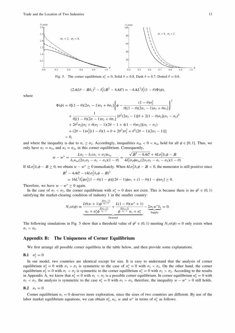
and where the inequality is due to �1 � �2. Accordingly, inequalities n2b < 0 < n2a hold for all � 2 ½0; 1�. Thus, weonly have n1 ¼ n1a and n2 ¼ n2a in this corner equilibrium. Consequently,

w�w� ¼L�2 � �1ð�1 þ �2Þn1a

�1n1að2�1�2 � �1 � �2Þð1� �Þ¼

ffiffiffiffiffiffiffiffiffiffiffiffiffiffiffiffiffiffiffiffiffiffiB2 � 4ACp

þ 4L�22�1��B

4�21�2�n1að2�1�2 � �1 � �2Þð1� �Þ:

If 4L�22�1��B � 0, we obtain w� w� � 0 immediately. When 4L�2

2�1��B < 0, the numerator is still positive since

B2 � 4AC� ð4L�22�1��BÞ2

¼ 16L2�21��32ð1� �Þð1� �Þ½ð2� � 1Þ��1 þ ð1� �Þð1� �Þ�2� � 0:

Therefore, we have w� w� � 0 again.In the case of �1 < �2, the corner equilibrium with n�1 ¼ 0 does not exist. This is because there is no �] 2 ð0; 1Þ

satisfying the market-clearing condition of industry 1 in the smaller country:

N1stð�Þ �L�ðwþ 1Þ�

�ð�1�1Þ�2�1

n1 þ n�1��ð�1�1Þ�2�1

þLð1� �Þðw� þ 1Þ

��ð�1�1Þ�2�1 n1 þ n�1|fflfflfflfflfflfflfflfflfflfflfflfflfflfflfflfflfflfflfflfflfflfflfflfflfflfflfflfflfflfflfflfflffl{zfflfflfflfflfflfflfflfflfflfflfflfflfflfflfflfflfflfflfflfflfflfflfflfflfflfflfflfflfflfflfflfflffl}

Demand

� 2�1w��1|fflfflfflffl{zfflfflfflffl}

Supply

¼ 0:

The following simulations in Fig. 5 show that a threshold value of �] 2 ð0; 1Þ meeting N1stð�Þ ¼ 0 only exists when�1 > �2.

Appendix B: The Uniqueness of Corner Equilibrium

We first arrange all possible corner equilibria in the table below, and then provide some explanations.

B.1 n�2 ¼ 0

In our model, two countries are identical except for size. It is easy to understand that the analysis of cornerequilibrium n�2 ¼ 0 with �1 > �2 is symmetric to the case of n�1 ¼ 0 with �1 < �2. On the other hand, the cornerequilibrium n�2 ¼ 0 with �1 < �2 is symmetric to the corner equilibrium n�1 ¼ 0 with �1 > �2. According to the resultsin Appendix A, we know that n�2 ¼ 0 with �1 < �2 is a possible corner equilibrium. In corner equilibrium n�2 ¼ 0 with�1 < �2, the analysis is symmetric to the case n�1 ¼ 0 with �1 > �2, therefore, the inequality w� w� > 0 still holds.

B.2 n1 ¼ 0

Corner equilibrium n1 ¼ 0 deserves more exploration, since the sizes of two countries are different. By use of thelabor market equilibrium equations, we can obtain n�2, n2, w and w� in terms of n�1 as follows.

σ1 2, σ2 8.

0.0 0.2 0.4 0.6 0.8 1.0φ

0.5

1.0

1.5

2.0

2.5

3.0N1st φ

σ1 8, σ2 2.

0.4 0.5 0.6 0.7 0.8 0.9 1.0φ

20

40

60

80

100N1st φ

Fig. 5. The corner equilibrium n�1 ¼ 0, Solid � ¼ 0:8, Dash � ¼ 0:7, Dotted � ¼ 0:6.

Trade and the Location of Two Industries 13

n2 ¼L�

�2; n�2 ¼

Lð1� �Þ�2

� n�1�1

�2; ðB:1Þ

w� ¼L�2

�1n�1ð2�1�2 � �1 � �2Þ; w ¼

�1n�1ð�1 þ �2Þ � Lð1� �Þ�2

��1n�1ð2�1�2 � �1 � �2Þ:

Plugging the equations above into the following market-clearing condition for industry 2

N2stð�Þ �L�ð1þ wÞ�n2 þ n�2�

þLð1� �Þ 1þ w�ð Þ

�n2 þ n�2� 2�2w

��2 ¼ 0;

obtains An�21 �B1n�1 þ C1 ¼ 0, where

B1 � L�1f� ð1� �Þ �1 þ �2ð Þ þ 2��1�2 þ 2�22

� �2

þ 2ð1� �Þ�2 �1 þ 2�2ð Þ�þ � ð1� �Þ�1 2�2 � 1ð Þ þ �2 2�2 � 1þ �ð Þ½ �g > 0;

C1 � L2�2 2�2ð� þ �� ��Þð1� � þ ��Þ � ð1� �Þ 1� �2 �

��

> 0:

This quadratic function of n�1 has two roots

n�1 ¼ n�1a �B1 �

ffiffiffiffiffiffiffiffiffiffiffiffiffiffiffiffiffiffiffiffiffiffiffiffiB2

1 � 4AC1

q2A

> 0 and n�1 ¼ n�1b �B1 þ

ffiffiffiffiffiffiffiffiffiffiffiffiffiffiffiffiffiffiffiffiffiffiffiffiB2

1 � 4AC1

q2A

> 0:

In the case of n�1b, we have

n�2 ¼ n�2b �2ALð1� �Þ �B1�1 � �1

ffiffiffiffiffiffiffiffiffiffiffiffiffiffiffiffiffiffiffiffiffiffiffiffiB2

1 � 4AC1

q2A�2

;

from full employment condition. From the numerator we have a quadratic function in terms of �:

�1ð�Þ �2ALð1� �Þ �B1�1

L�21¼ 2�1�1 � �1 � �2ð Þ 1� �2

��2

� �1 þ �2ð Þ 2�2 � 1ð Þ þ 2�1�2�þ �1 þ �2 þ 2�22

��2

� � þ 2�1�2�:

For � 2 ð1=2; 1Þ, we have �1ð1Þ ¼ �2�2½�2 þ ð�1 þ �2Þ�2� < 0. On the other hand, we have

�1

1

2

� �¼ �

1

4�1 þ �2 þ 2�1�2 þ 4�2

2 �

�2 þ �1�2�þ1

4�1 þ �2 � 2�1�2 � 4�2

2 �

��1 þ �2ð Þ �1 þ �2 � 16�2

3 �

4 �1 þ �2 þ 2�1�2 þ 4�22

� < 0;

where the second inequality is due �1 � �2. Since ð2�1�1 � �1 � �2Þð1� �2Þ > 0, we know �1ð�Þ < 0 for � 2 ð1=2; 1Þby the properties of quadratic function. Accordingly, inequality n�2b < 0 holds for all � 2 ð0; 1Þ, so we only haven�2 ¼ n�2a in this corner equilibrium. However, we show that n�2 ¼ n�2a < 0 for � 2 ð�]; 1Þ. Note that �] is defined as thethreshold value of trade freeness that satisfies market-clearing condition of the industry 1 in the larger country:

N1ð�Þ �L�ðwþ 1Þ

n1 þ n�1��ð�1�1Þ�2�1

þLð1� �Þ w� þ 1ð Þ�

�ð�1�1Þ�2�1

��ð�1�1Þ�2�1 n1 þ n�1|fflfflfflfflfflfflfflfflfflfflfflfflfflfflfflfflfflfflfflfflfflfflfflfflfflfflfflfflfflfflfflfflfflfflfflfflffl{zfflfflfflfflfflfflfflfflfflfflfflfflfflfflfflfflfflfflfflfflfflfflfflfflfflfflfflfflfflfflfflfflfflfflfflfflffl}

Demand

� 2�1w�1|fflfflffl{zfflfflffl}Supply

¼ 0:

Although we have no closed-form solution of �], Fig. 6 shows that n�2a is negative when � 2 ð�]; 1Þ. It implies thatwhen �1 � �2, n1 ¼ 0 is not a plausible corner equilibrium.

In the case of �1 > �2, n1 ¼ 0 is not a possible corner equilibrium. Because the threshold value of �] 2 ð0; 1Þ whichsatisfies the market-clearing condition N1ð�Þ ¼ 0 does not exist. Figure 7 shows the result of our simulation. We cannot observe such a �] 2 ð0; 1Þ when �1 > �2.

B.3 n2 ¼ 0

By use of the symmetry of this model setting, we know that the analysis of corner equilibrium n2 ¼ 0 with �1 > �2 issymmetric to the case of n1 ¼ 0 with �1 < �2. On the other hand, the analysis of corner equilibrium n2 ¼ 0 with

Table 2. Types of corner equilibria. Possible: , Impossible: .

Corner equilibriumn�1 ¼ 0 n�2 ¼ 0 n1 ¼ 0 n2 ¼ 0

Demand elasticity

�1 > �2

�1 < �2

14 ZHOU et al.

�1 < �2 is symmetric to the case of n1 ¼ 0 with �1 > �2. According to the results in the above subsection, we knowthat n2 ¼ 0 is not a possible corner equilibrium.

REFERENCES

[1] Amiti, M., Inter-industry trade in manufactures: Does country size matter? Journal of International Economics 44: 231–255(1998).

[2] Chen, Q.-M. and Zeng, D.-Z., The spatial selection of heterogeneous quality: An approach using different demand elasticities.International Journal of Economic Theory, 10(2): 179–202 (2014).

[3] Davis, D. R., The home market effect, trade and industrial structure. American Economic Review 88: 1264–1276 (1998).[4] Helpman, E. and Krugman, P., Market Structure and Foreign Trade. MIT Press, Cambridge, MA (1985).[5] Krugman, P., Scale economies, product differentiation and pattern of trade. American Economic Review 70: 950–959 (1980).[6] Krugman, P., Increasing returns and economic geography. Journal of Political Economy 99: 483–499 (1991).[7] Krugman, P. and Venables, A., Globalization and the inequality of nations. Quarterly Journal of Economics 110: 857–880

(1995).[8] Laussel, D. and Paul, T., Trade and the location of industries: Some new results. Journal of International Economics 71: 148–

166 (2007).[9] Markusen, J., Trade and the gains from trade with imperfect competition. Journal of International Economics 11: 531–551

(1981).[10] Markusen, J. and Melvin, J., Trade, factor prices and the gains from trade with increasing returns to scale. Canadian Journal of

Economics 14: 450–469 (1981).[11] Martin, P. and Rogers, C. A., Industrial location and public infrastructure. Journal of International Economic 39: 335–351

(1995).[12] Peng, S.-K., Wang, P., and Thisse, J.-F., Economic integration and agglomeration in a middle product economy. Journal of

Economic Theory 131: 1–25 (2006).[13] Peng, S.-K. and Zeng, D.-Z., Globalization without industrial delocation, paper presented in the 15th Annual Conference of the

Association for Public Economic Theory, University of Washington, Seattle, July 10–13 (2014).[14] Takahashi, T., Takatsuka, H., and Zeng, D.-Z., Spatial inequality, globalization and footloose capital. Economic Theory 53:

213–238 (2013).[15] Takatsuka, H. and Zeng, D.-Z., Trade liberalization and welfare: differentiated-good versus homogeneous-good markets.

Journal of the Japanese and International Economies 26: 308–325 (2012a).[16] Takatsuka, H. and Zeng, D.-Z., Mobil capital and the home market effect. Canadian Journal of Economics 45: 1062–1082

(2012b).

σ1 3, σ2 5

n2 a

N1 φ

0.2 0.4 0.6 0.8 1.0φ

0.5

0.5

1.0

1.5

2.0N1 φ ,n2

Fig. 6. n�2 < 0 when � 2 ð�]; 1Þ, Solid � ¼ 0:8, Dash � ¼ 0:7, Dotted � ¼ 0:6.

σ1 5, σ2 3.

0.4 0.5 0.6 0.7 0.8 0.9 1.0φ

2

4

6

8N1 φ

σ1 8, σ2 5

0.4 0.5 0.6 0.7 0.8 0.9 1.0φ

1

2

3

4

5

6

7N1 φ

Fig. 7. The corner equilibrium n1 ¼ 0 with �1 > �2, Solid � ¼ 0:8, Dash � ¼ 0:7, Dotted � ¼ 0:6.

Trade and the Location of Two Industries 15