Trade barriers and export potential: Gravity estimates for Norway’s exports Arne Melchior, Jinghai Zheng and Åshild Johnsen, NUPI Paper written for the Ministry of Trade and Industry, Norway Oslo, May 2009 Abstract Using trade and tariff data for around 150 countries, we estimate the impact of tariffs on Norway’s exports to these countries in 2007. Remaining tariffs have a significant and measurable impact on exports: on average a one percent tariff reduces exports by around 4 percent. Using these estimates to assess the trade potential from tariff elimination, we find that trade may increase by 4.2-12.9 billion NOK, equivalent to 1.2-3.7% of Norway’s non-oil exports in 2007. The trade potential is largest for the BRICs and the USA, and for the sectors minerals, fish, machinery and chemicals. Some countries also have high non-tariff barriers; in some cases even higher than their tariff barriers.
Transcript
Trade barriers and export potential: Gravity estimates for Norway’s exports Arne Melchior, Jinghai Zheng and Åshild Johnsen, NUPI Paper written for the Ministry of Trade and Industry, Norway Oslo, May 2009 Abstract Using trade and tariff data for around 150 countries, we estimate the impact of tariffs on Norway’s exports to these countries in 2007. Remaining tariffs have a significant and measurable impact on exports: on average a one percent tariff reduces exports by around 4 percent. Using these estimates to assess the trade potential from tariff elimination, we find that trade may increase by 4.2-12.9 billion NOK, equivalent to 1.2-3.7% of Norway’s non-oil exports in 2007. The trade potential is largest for the BRICs and the USA, and for the sectors minerals, fish, machinery and chemicals. Some countries also have high non-tariff barriers; in some cases even higher than their tariff barriers.
1
Non-technical summary The paper uses a gravity model to assess the impact of tariff barriers on Norway’s exports, and thereafter uses these estimates in order to predict how trade would change if tariffs in export markets were eliminated. For this purpose, a large-scale database is constructed, including trade and tariffs facing Norway’s exports in more than 150 countries. The analysis is based on Norwegian export data but there are generally huge gaps between Norway’s reported exports and the imports from Norway reported by countries at the other end. Some of the gap can be caused by weaknesses in Norwegian data.
If Norway had faced regular tariffs in all export markets, the tariff burden for current exports in 2007 would have been 1.6 billion USD. Due to free trade agreements in many major markets, however, tariffs were lower so the actual tariff burden was only 54 million USD. This is however an underestimate of the true tariff burden since trade tends to be low when tariffs are high. For oil and gas exports, there were no tariffs at all. Taking simple country-level tariff averages for goods exported to all countries in the sample, we find that the mean as well as the median across countries is around 7%.
Through EFTA and the EEA (European Economic Area) Agreement, Norway currently has free trade agreements (FTAs) with 51 countries. In addition, negotiations aiming at new FTAs are currently going on with another 14 countries. If all these negotiations succeed, around 90% of Norway’s foreign trade will be with FTA partners. The current share is around 85%.
We use a modified “gravity model” in order to measure how tariffs affect exports, along with geographical distance and the size of the destination markets (measured by GDP). Estimates vary across sectors and their absolute values are generally higher if we use aggregated trade data, as opposed to data at the detailed product level. Due to this variation, we indicate a range with lower and upper bounds for the “tariff elasticity” for each main sector. On average, we find that a 1% tariff reduces exports by around 4%. Hence tariffs have a relatively large and measurable trade-reducing effect.
Based on these estimates, we estimate how exports would change if tariffs were eliminated, for exports to more than 150 countries. Summed across all these countries, we find that exports may increase by 4.2-12.9 billion NOK, equivalent to 1.2-3.7% of Norway’s non-oil exports in 2007. The trade potential is largest for the BRICs (Brazil, Russia, India and China) and the USA, and for the sectors minerals, fish, machinery and chemicals. Fish and machinery face higher tariffs, but minerals are more price-sensitive so even low tariffs can have a large impact.
We also report results from other studies on non-tariff barriers (NTBs). Some countries have high NTBs even if their tariffs are low, and this should be taken into account in free trade negotiations.
As a check of our estimates, we undertake retrospective trade potential estimates for some countries where Norway established FTAs earlier. We calculate trade potentials after the entry into force of the various agreements, also taking into account GDP growth. Comparing these predictions with actual trade growth, we find the predictions are in the right order of magnitude. There are however substantial deviations which demonstrate that trade is affected by a number of aspects that are not captured by the gravity model.
2
1. Introduction* In spite of considerable trade liberalisation over time, Norway’s exports of goods still face significant tariff and non-tariff barriers. Figure 1 shows simple tariff averages for 135 countries using data mainly for 2007, for goods actually exported to each market. While tariffs are zero in eight markets, the median as well as the average value was around 7%. This also takes into account preferential tariffs in Norway’s free trade agreements.
Figure 1: Tariffs facing Norwegian exports in 135 countries Data sources: See Appendix A.
0
5
10
15
20
25
30
35
1 21 41 61 81 101 121
Sim
ple
tarif
f ave
rage
It is generally the case that poor countries have higher tariffs than rich ones, and globalisation implies increased trade with developing countries across the globe. Norwegian firms therefore face significant tariffs in a number of markets. Tariffs may be reduced by means of WTO liberalisation, free trade agreements or unilateral tariff reductions by each country. In the current Doha Round negotiations of the WTO, there are proposals to cut tariffs but the failure of the round so far renders it uncertain when and even whether these reductions will be undertaken. This is one reason why a number of countries pursue free trade agreements (FTAs) in which tariff elimination or reduction is one important objective. Norway participates in a number of FTAs as part of the EEA (European Economic Area) which currently covers EU-27 plus the EFTA countries Iceland, Norway and Liechtenstein (Switzerland does not participate in the EEA). In addition, Norway has 17 FTAs through EFTA; with Canada, Chile, Colombia, Croatia, Egypt, Israel, Jordan, Lebanon, Macedonia, Mexico, Morocco, Palestine Territory, Singapore, SACU (South African Customs Union, including Botswana, Lesotho, Namibia, Swaziland and South Africa), Korea, Tunisia and Turkey.1 EFTA
* Funding from the Ministry of Trade and Industry is gratefully acknowledged and we thank the Ministry for comments to an earlier draft. In the project, Åshild Johnsen worked as research assistant responsible for data. 1 As of May 2009, the agreements with some of these countries had not yet entered into force. This applies to Canada (expected to enter into force on 1 July 2009) and Colombia (signed November 2008, pending ratification).
3
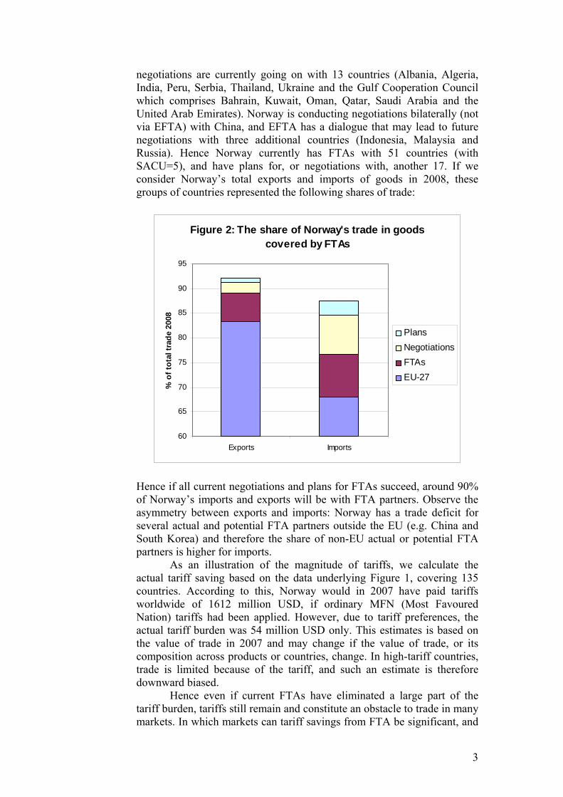
negotiations are currently going on with 13 countries (Albania, Algeria, India, Peru, Serbia, Thailand, Ukraine and the Gulf Cooperation Council which comprises Bahrain, Kuwait, Oman, Qatar, Saudi Arabia and the United Arab Emirates). Norway is conducting negotiations bilaterally (not via EFTA) with China, and EFTA has a dialogue that may lead to future negotiations with three additional countries (Indonesia, Malaysia and Russia). Hence Norway currently has FTAs with 51 countries (with SACU=5), and have plans for, or negotiations with, another 17. If we consider Norway’s total exports and imports of goods in 2008, these groups of countries represented the following shares of trade:
Figure 2: The share of Norway's trade in goods covered by FTAs
60
65
70
75
80
85
90
95
Exports Imports
% o
f tot
al tr
ade
2008
PlansNegotiationsFTAsEU-27
Hence if all current negotiations and plans for FTAs succeed, around 90% of Norway’s imports and exports will be with FTA partners. Observe the asymmetry between exports and imports: Norway has a trade deficit for several actual and potential FTA partners outside the EU (e.g. China and South Korea) and therefore the share of non-EU actual or potential FTA partners is higher for imports.
As an illustration of the magnitude of tariffs, we calculate the actual tariff saving based on the data underlying Figure 1, covering 135 countries. According to this, Norway would in 2007 have paid tariffs worldwide of 1612 million USD, if ordinary MFN (Most Favoured Nation) tariffs had been applied. However, due to tariff preferences, the actual tariff burden was 54 million USD only. This estimates is based on the value of trade in 2007 and may change if the value of trade, or its composition across products or countries, change. In high-tariff countries, trade is limited because of the tariff, and such an estimate is therefore downward biased.
Hence even if current FTAs have eliminated a large part of the tariff burden, tariffs still remain and constitute an obstacle to trade in many markets. In which markets can tariff savings from FTA be significant, and
4
where is the trade gain from tariff elimination potential largest? In order to shed light on this question, this paper analyses the impact of tariffs on Norway’s current exports, and thereafter uses these estimates in order to predict how trade might change if tariffs in selected markets are eliminated.
Maurseth (2003) presented a similar analysis using tariff data for 1999. Using a modified gravity model, Maurseth estimated “tariff elasticities” for various product groups and used these to predict potential trade changes if tariffs were eliminated. In this paper, we start by replicating Maurseth’s analysis as a benchmark, using more recent data for a larger sample of countries. While Maurseth had disaggregated tariff data for 41 countries, such data are now available for around 150 countries. We thereafter extend the analysis in various ways. Maurseth used general MFN tariffs, but our data reflect tariff preferences (FTAs). We also modify the analysis methodologically in some respects.
The paper proceeds as follows: In section 2 we present the data and some descriptive statistics. Section 3 addressed the gravity model and the forms used in the regression analysis. Section 4 presents regression results, and section 5 contains estimates of the trade potential if tariffs are eliminated for selected countries. Section 6 discusses the role of Non-Tariff Barriers (NTBs) compared to tariffs and uses some international estimation results in order to shed light on the magnitudes involved. In Section 7, we look back in time and examine ex post how trade predictions compare to real trade developments, for countries where Norway have agreed on FTAs after 1990. Section 8 concludes. 2. The data A large database has been constructed for the project. In Appendix A, more information about classification and data is provided. The main sources of data are the following: - Trade data are from the COMTRADE database of the United Nations,
using the WITS (World Integrated Trade Solution) software provided by UNCTAD and the World Bank.
- Tariff data are mainly taken from UNCTAD’s TRAINS database, also using WITS.
- Data on geographical distance are constructed from coordinates taken from the Global Cities database.
- Country data (GDP, GDP per capita etc.) are taken from the World Bank’s WDI (World Development Indicators), online version 2009.
In general, the data set is constructed using the most detailed classification available for trade in goods at the international level; the 6-digit level of product classification. At this level, there are approximately 5000 products so a complete tariff data set for an individual country contains this number of observations.2 Combining all countries in one large tariff data set we have 775 000 observations. There are however exports from Norway in a minority of cases, so using data with observed exports from Norway we
2 Countries may have even more detailed classifications at the national level; e.g. Norway uses eight digits (see e.g. Melchior 2006 for information).
5
end up with 45 414 observations. This is the file used in the gravity regressions. We also run some regressions where trade is aggregated into one single observation for each country. The number of countries included in the regressions is maximum130 (due to some missing observations). In addition there are around 20 other countries for which tariff data are available and where it is possible to calculate the trade potential if tariffs are eliminated, using the parameter estimates obtained from regressions. While the regressions are generally based on Norwegian export data, we use in some calculations Norway’s market share as a parameter and for that purpose we have to use import data reported by the various export partners. In principle, Norway’s exports of a product to some country should be similar to this country’s imports of that product from Norway, save for the difference caused by transport and handling costs.3 When comparing export and import data, however, we found huge gaps. This is illustrated in Figure 3, where we show each country’s total imports from Norway as a percentage of Norway’s total reported exports to that country in 2007.
Figure 3: Reported imports from Norway as % of Norway's reported exports to each country, 2007
If statistics were matching, the bulk of observations should be around 100% or slightly higher, but this is the case only for a small number of countries. For most countries there are considerable gaps. As an alternative, we considered to use the BACI database of harmonised international trade data, constructed by CEPII, France (www.cepii.fr). The latest year of trade in BACI is however 2005, and since a purpose of the analysis was to provide updated figures, we have chosen to use the COMTRADE export and import 2007 data simultaneously in some cases. Some caution should therefore be exercised with respect to the quality of the trade data. While the Norwegian instinct would be that Norwegian data are excellent and other countries’ data poor, this is not fully supported by
3 Technically, export values are f.o.b. (free on board) where as import values are c.i.f. (cost, insurance, freight included).
6
the evidence: According to CEPII, Norway is in the mid-range of the better group with respect to data quality (Gaulier and Zignago 2008). In the TRAINS database, tariffs are reported in different forms: - Bound tariffs (BND) are those negotiated in WTO and they constitute
upper bounds for the applied tariffs. - MFN applied tariffs are those actually applied to countries that have no
special tariff preferences in a given market. - Preferential tariffs (PRF) include tariffs in preferential trade
agreements. The coverage of such tariffs in international databases has increased in recent years. In the regressions to be undertaken, we have data for most of the countries for which Norway has FTAs. Observe that PRF tariffs are reported only where such preferences exist and in order to obtain a full set of tariffs for all traded products, we have to fill in with MFN tariffs in cases where there are no preferences. The set of tariffs named PRF in the following is therefore a mixture of preferential and MFN tariffs.
- In addition, the TRAINS database reports an average (AHS) tariff which uses the tariff actually applied for each country. Hence if one asks for the AHS tariff for imports from the world for a certain product, one obtains an average of MFN and preferential tariffs.
In Figures 4 and 5 we report simple and weighted tariff averages for across products and countries, for 12 main sectors. The sector classification is provided in Appendix B, and Appendix A contains information on how averages are calculated.
Figure 4: Simple averages of tariffs facing Norway's exports in 2007, by main sectors
0 10 20 30 40 50
Oil
Chemicals
Machinery
Metal
Instruments
Minerals
Wood
Transport eq.
Fish
Textiles
Food
Lightind.
Simple tariff average
BoundMFNAveragePreferential
7
Figure 5: Weighted average of tariffs facing Norway's exports in 2007, by main sectors
0 1 2 3 4 5 6 7 8
Oil
Wood
Lightind.
Metal
Chemicals
Transport eq.
Minerals
Instruments
Textiles
Machinery
Fish
Food
Weighted tariff average
BoundMFNAveragePreferential
According to the simple averages, bound tariffs are far higher than all other tariff types; illustrating that WTO negotiations are to a considerable extent about “water in the tariffs”. For many countries, large tariff cuts are required before bound tariffs get down to the MFN applied tariff level. According to the simple averages, there is not much difference between MFN, average and Norway’s tariffs including preferences. This is because there are no preferences for the majority of product/country observations in the sample. When weighted by Norway’s exports, however, all tariff levels are substantially reduced and the relative difference between PRF, AHS and MFN increases. In most sectors, tariff preferences for existing trade are substantial. This is mainly driven by the preferences in the European markets. However, Figure 5 also shows that Norway is not the only country having preferences: In many cases, AHS is mid-way between MFN and PRF, suggesting that many other countries also have tariff preferences. For example, Norway has obtained substantial tariff cuts for “white fish” such as cod in the EU market, but a closer look reveals that almost all other significant suppliers have at least as good preferences in the EU market (Melchior 2007). Hence even when the MFN tariff is high and the PRF tariff is zero, the relative preference or discrimination effect may be limited. In some markets, it could also be the case that AHS is lower than PRF, if other countries have preferences but not Norway. The ranking of sectors differs in Figures 4 and 5. According to weighted averages, food, fish and machinery are sectors facing higher tariffs. Since exports of food products are more limited, one may expect a larger trade potential for fish and machinery if tariffs are reduced. We will see later that this is indeed the case.
8
Observe that trade-weighted tariff averages for oil products are zero, except for the bound tariffs. Hence there is no trade potential for oil if tariffs are reduced, and we obtain no estimates for “tariff elasticities” in the regressions to be undertaken. 3. The gravity model Ever since its introduction by Linnemann (1966), the gravity model has been a workhorse for applied work on international trade. In spite of some ambiguity about the model’s trade-theoretical foundation, it is an astonishingly robust empirical relationship that has prevailed in spite of changing focus in trade theory. The basic form of the gravity equation is as follows: (1) ln(Tradeij) = α + βi * ln(GDPi) + βj * ln(GDPj) + γ * ln(Distanceij) Depending on the specification, Tradeij can be exports from country i to country j, or total trade (exports + imports) between the two countries. In the former case, we use subscript i for the exporter and j for the importer. The β parameters then measure the impact of exporting and importing country size, and γ measures the impact of distance. The gravity model can be rationalised within different theoretical approaches. Total supply and demand tend to increase with country size and with suitable functional forms this may generate trade as a “multiplicative” function of the two GDPs. In the new trade theory, country size also affects comparative advantage due to “home market affects” and this adds another potential explanation of gravity. The new economic geography adds another layer since GDP levels may depend on location and distance. A next step in developing theoretical approaches to gravity may be to incorporate this perspective properly; which has been done only to a limited extent. When the gravity equation is used for exports + imports, the estimates on GDP are usually symmetrical; of equal size, positive and normally somewhat below one. If the gravity model is applied for trade at the sector level, however, the estimates βi and βj on GDP may differ. If large countries have an advantage in the production of some goods due to scale economies, as predicted by the new trade theory, we will generally have βi > βj (see e.g. Melchior 1996 or Feenstra, Markusen and Rose 2001).
The distance parameter γ is normally negative, with estimates ranging from -0.28 to -1.55 with a typical outcome around -0.9 (Disdier and Head 2008).Distance is just a proxy for various trade costs that depend on distance and if other trade cost variables are added, the absolute value of the distance parameter could be reduced. In principle, the distance parameter could become insignificant if we are able to measure all trade barriers correctly. When comparing gravity regressions from the 1950s and recent ones, the distance parameter estimates has not changed much and some have interpreted this as the “missing globalisation puzzle”. However, γ measures the elasticity or relative effect, and not the level, so if all transport costs are reduced by half there is no reason to expect this parameter to change (see Buch et al. 2004 for a discussion).
9
A hidden problem in the gravity model is that GDP may depend on geography, for example if centrally located countries have higher GDP levels due to a better location. Hence GDP may be endogenous and depend indirectly on distance. A first step towards correction for such biases is to include a term in the gravity equation that captures location, for example a market potential variable measuring “remoteness” (see e.g. Anderson and Wincoop 2003). In recent years there has been vivid discussion also concerning other methodological issues related to gravity; see e.g. Baldwin and Taglioni (2006) for a useful contribution. One such issue is how to handle zero observations: In a bilateral trade matrix between many countries there are many zeros and unless one takes them into account, estimates could potentially be biased.
The problem of “remoteness” is more serious if we estimate the gravity equation with multilateral data for many countries. In our case, we will use data for Norway’s exports only and the equation changes to: (2) ln(exportskj) = αk + βk * ln(GDPj) + γk * ln(Distancej) Where the i subscripts have been dropped since they will be common to all observations, but we have added a subscript k since we will run regressions for different sectors k. Hence we can check whether the estimates βk and γk vary across sectors. We now follow Maurseth (2003) by adding a tariff term to the gravity equation, which becomes (3) ln(exportskj) = αk + βk * ln(GDPj) + γk * ln(Distancej) + μk * ln(tkj) The tariff term tkj refers to the tariff in country j for sector k. We have tariffs at the 6-digit product level, but group these into 12 main sectors k. In Appendix B, the sector definition is provided. We will undertake some regressions using aggregate sector trade data and average tariffs for the sector, and some regressions at the product level. For the aggregate sector regressions, the number of observations depends on the number of countries in the sample (maximum around 130 due to missing data for some variables). When running disaggregated regressions, we assume that the parameter estimates are common to all products within a sector.
With disaggregated regressions there is a problem involved in (3) since it mixes products with different magnitudes. For example, the fish sector contains salmon which is exported in large volumes and values to many countries, along with some product with small exports to a few countries only. Maurseth (2003) took this into account by adding the total exports of each product as a right hand side variable, in logs. Maurseth also included the log of GDP per capita in the equation, given that tariffs and income levels are correlated and there could be an omitted variable bias unless the income level is taken into account. The equation then becomes (4) ln(exportskpj) = αk + βk * ln(GDPj) + γk * ln(Distancej) + μk * ln(tkpj)
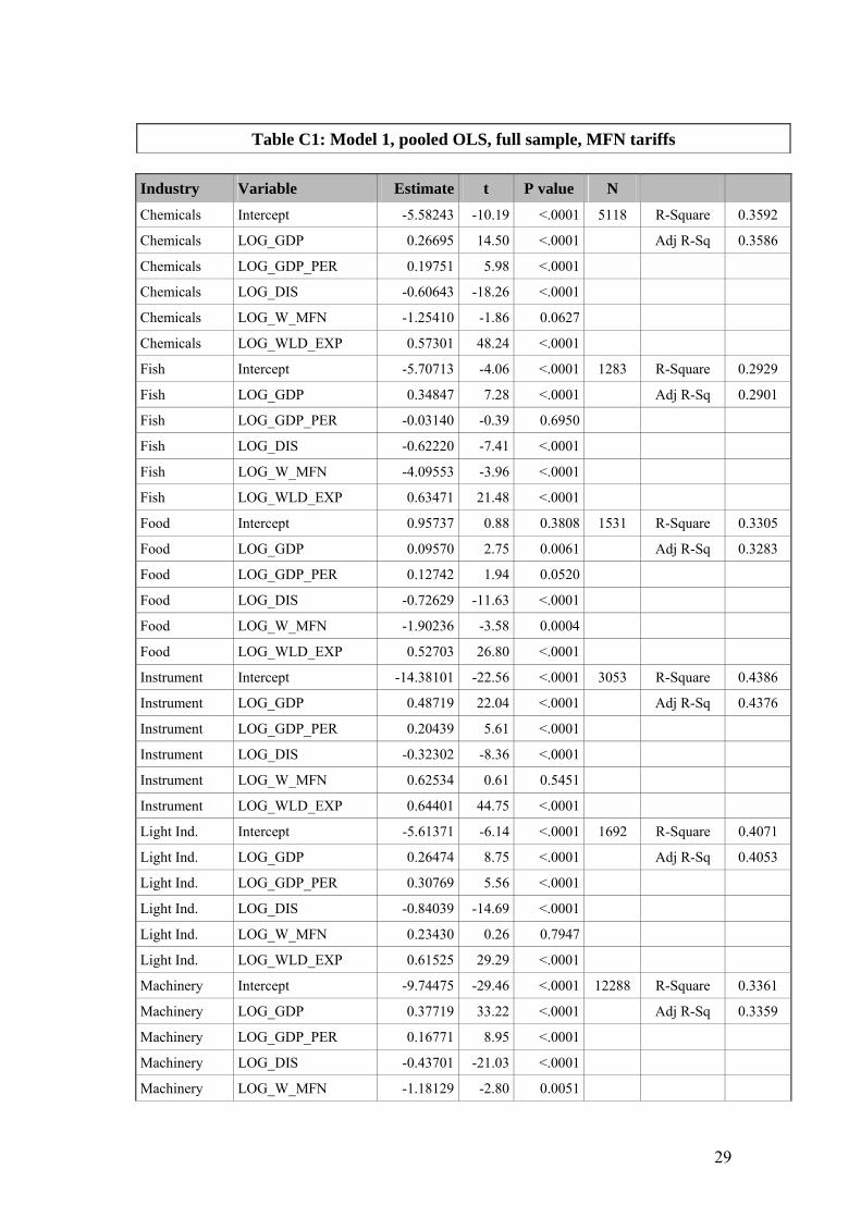
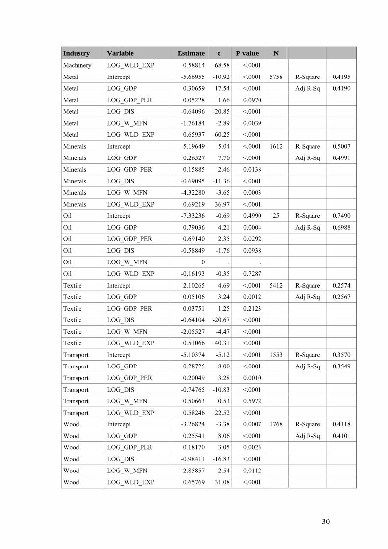
where subscript p are added in three of the terms. We use this as a starting point and benchmark, which we will later modify and elaborate. Note that in the regressions, tariffs are always expressed in the form (5) ln(tkj) where tkj = (100+TARIFFkj)/100 Hence if the tariff is 10%, tkj is 1.1. If the tariff is zero, we have tkj=1 and ln(tkj)=0. Using this form, the parameter μk can be interpreted as an ordinary elasticity; a 1% tariff change is approximately equivalent to a 1% change in the price. 4. Regression results As a starting point, we replicate the results of Maurseth (2003) with disaggregated data at the product level, using equation (4). We will refer to this as “Model 1”. Table C1b in the Appendix shows the results. Table C1a in the Appendix compares the main parameter estimates with those obtained by Maurseth (2003).
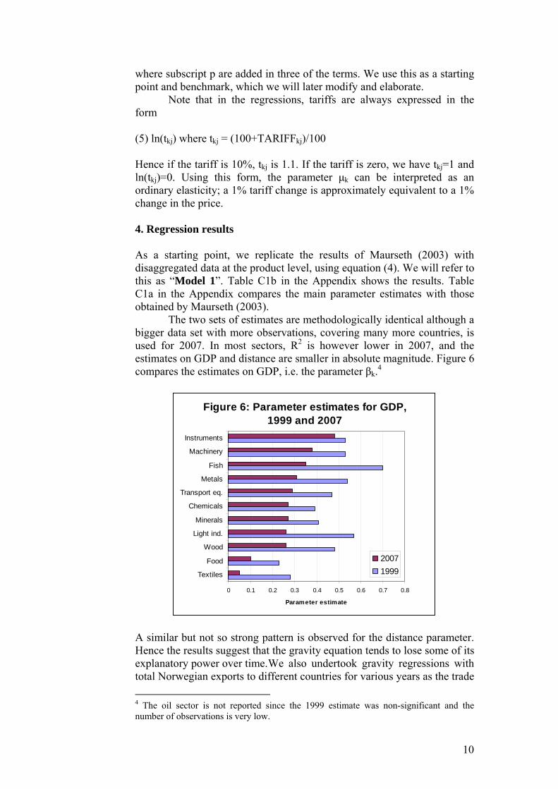
The two sets of estimates are methodologically identical although a bigger data set with more observations, covering many more countries, is used for 2007. In most sectors, R2 is however lower in 2007, and the estimates on GDP and distance are smaller in absolute magnitude. Figure 6 compares the estimates on GDP, i.e. the parameter βk.4
Figure 6: Parameter estimates for GDP, 1999 and 2007
0 0.1 0.2 0.3 0.4 0.5 0.6 0.7 0.8
Textiles
Food
Wood
Light ind.
Minerals
Chemicals
Transport eq.
Metals
Fish
Machinery
Instruments
Parameter estimate
20071999
A similar but not so strong pattern is observed for the distance parameter. Hence the results suggest that the gravity equation tends to lose some of its explanatory power over time. We also undertook gravity regressions with total Norwegian exports to different countries for various years as the trade 4 The oil sector is not reported since the 1999 estimate was non-significant and the number of observations is very low.
11
variable (not reported here), and these confirmed this trend: At least for Norway, the gravity equation tends to lose some of its explanatory power over time. Detecting the reasons for this is an interesting task for further research: Has the “world become smaller” so that distance becomes less important, or have scale economies become less important so that country size matters less for the trade pattern? In spite of this deterioration in the fit of the gravity equation, parameter estimates are in general still highly significant and the model can be used for our purpose: To estimate the impact of tariff barriers. Turning to tariffs, the elasticities reported in Table C1 and C2 are mixed both for the 1999 and 2007 results: Some are higher in 2007, and some lower. Some are non-significant and some even positive. More work is therefore needed in order to provide a more reliable assessment of the tariff impact. The Model 1 estimates use MFN tariffs which do not actually apply to Norwegian exports and this may be cause biased results. We therefore introduce preferential tariffs, and also undertake other modifications of the model. In the following, we will report five other regressions, named Model 2- Model 6. Their motivation is explained in the following. Model 1 uses product-level data and for many products, exports are limited and concentrated on very few markets. In the data set, we observe exports of 3746 products from Norway in 2007 but for many of these, the number of export markets is very limited. Figure 7 shows the frequency distribution.
Figure 7: The number of export markets per product
0
100
200
300
400
500
600
0 20 40 60 80 100 120
Number of export markets
Num
ber o
f pro
duct
s
The horizontal axis shows the number of export markets (countries) per product and we see that more than 500 products were sold only one market. In these cases, the right hand side variable for total product exports will be identical to the independent variable, which is clearly an econometric problem potentially causing a bias. If we had run the regressions for these 500 products only, the total export variable would “explain” 100% of the variation in exports and the other variables would contribute little. Furthermore, we try to measure the impact of tariffs across markets but for these products there is clearly no variation in tariffs
12
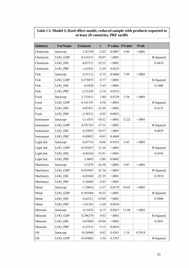
since there is only one tariff observation. Such variation is also limited for many other products that are sold to only a few markets. Products sold to less than 20 countries represent 81% of the products and 43% of the observations. In order to address this problem; in Model 2 we delete all products sold to less than 20 countries; thus reducing the number of observations by 43%. We could also have used a lower threshold but even with a threshold at 20 markets we have sufficient degrees of freedom. We try three different specifications: Pooled regressions maintaining the total product export variable on the right hand side, or panel (fixed and random) models where we drop the total export variable. There was however little difference between the three, and we therefore report the pooled OLS regression since it is easier to use for predictions of the trade potential later (since we do not have to use product-level dummies). The results on tariffs from Model 2 are significant in more cases and the absolute value of the elasticities is on average higher. Still, however, there is uncertainty about the results since we use MFN tariffs, that actually do not apply to Norway’s exports. In Model 3 we therefore use preferential tariffs. We experiment with different specifications including pooled OLS as well as panel methods (e.g. with fixed or random effects for products, and with the reduced sample used in Model 2). There are not big differences across specifications, and we report OLS with the whole sample. Maybe surprisingly (since we now use PRF tariffs), the tariff elasticity estimates are not consistently higher compared to Models 1 and 2, but slightly lower. A possible limitation of models 1-3 is that we do not distinguish between tariff cuts in the context of FTAs, and tariff cuts that apply to all suppliers. This distinction may be particularly important since a purpose is to evaluate the impact of potential FTAs. If Norway obtains privileged tariff cuts in a market, it can take over market shares from other suppliers worldwide. On the other hand if tariff cuts are given to all suppliers, such market share responses will be limited; all exporters may increase their supply by taking over shares from domestic suppliers. In the regressions, we try to address this problem in various ways. One is to introduce a variable that measures the relative preference in a market. The difference between the average actually applied (AHS) tariffs and the PRF (preferential) tariffs may be used as an approximation to the relative tariff preference. In equation 6 we replace the tariff term in equation (4) with two new terms; one measuring the general tariff level in a market (using AHS), and one measuring the relative preference of Norway (using the ratio tkpj-PRF/tkpj-AHS). (6) ln(exportskpj) = αk + βk * ln(GDPj) + γk * ln(Distancej) + μk * ln(tkpj-AHS) + θk *ln(tkpj-PRF/tkpj-AHS) + λk * ln(exportsp) + residualkpj Attempting this specification, we obtained some results in line with the prediction; e.g. for machinery we find an elasticity for the first terms of -2.49 and an elasticity for the relative preference term at -7.67. Similar results were found for five other sectors but only in one case were both estimates statistically significant at the same time. Running regressions
13
with the relative preference term alone (see e.g. Hoekman and Nicita 2008 for an approach along these lines) did not improve results either; probably since then we miss the impact of the tariff level as such.
We therefore try an indirect route in order to assess the impact of preferences: A common approach in modern modelling of demand is two-step budgeting where consumers first choose between aggregates; and thereafter between varieties within each aggregate. In the context of Norwegian exports, we may think of a market where consumers in the first step choose their spending on some product (say some species of fish); and thereafter between different varieties of this (say Norwegian or Chilean salmon). Now the point is that the substitution elasticity between products (step 1) should be lower than between varieties of the product. Using a so-called CES function at the second step, we can derive the formula
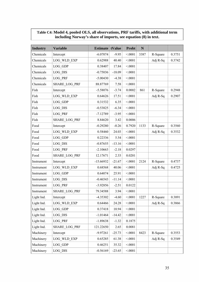
(7) eNj = -σi + sNj * (σi-εi) where σi is the “substitution elasticity” between suppliers in market j, sNj is the market share of Norway in market j and εi is the demand elasticity for the product in market j. If Norway has the whole market (market share = 1) it is not possible to take shares from others so the elasticity is equal to εi. But if the market share is zero, a tariff cut for Norway can make it possible to take shares from others, so the elasticity will be σi. Kee et al. (2008) estimate more than 377 000 (!) import demand elasticities and find a global average across products and markets of -3.12. This covers all imports to a country so it does not correspond directly to any of the terms in (7). According to the literature, the elasticity of substitution could typically be around 5 while the demand elasticity might be around 1-1.5. For a preferential agreement the appropriate value should be between, but more likely closer to the higher end. If the demand elasticity εi is used, one may underestimate the trade potential. As an attempt to capture this, we calculate the share of Norway in the total imports for each country/product and use the following specification: (8) ln(exportskpj) = αk + βk * ln(GDPj) + γk * ln(Distancej) + μk * ln(tkpj-PRF) + θk * skJ * ln(tkpj-PRF) + residualkpj We then expect the parameter μk to be negative and the parameter θk to be positive. We estimate this using ordinary OLS as well as fixed and random effects. The results from differet approaches are similar and we report the OLS estomates. This is Model 4, with detailed results provided in Table C4 in the Appendix.
14
Table 1: Estimates indicating that the elasticity depends on market share Selected results from Model 4 estimation. Details are in Table C4 in the appendix.
Note: Significance levels indicated by *** (P value<0.01), ** (0.01<P value<0.05). The parameter to the left should in principle capture the elasticity of substitution, while the second parameter captures the last term in (7). In order to find the demand elasticity for Norway’s exports, we use (7) at the product level and then calculate simple averages across products.
Models 1-4 are all estimated with disaggregated data at the product level. Some potential problems have been discussed but there may be even more problems due to the heterogeneity. We have tried panel approaches but there are some problems involved due to the highly unbalanced nature of the data, with the number of countries per product as well as the number of products per country varying strongly. With disaggregated data there may also be greater problems with outliers as well as data errors. As an attempt to address these issues we therefore also estimate the elasticities using aggregate data at the sector level. In this case we do not need dummies or variables correcting for heterogeneity across product, and we can run a simple cross-section. The number of observations now depends on the number of countries, and the maximum in a sector is 130. In Model 5 we use MFN tariff data, and in Model 6 we use preferential tariffs. The detailed results are found in Tables C5-C6 in the Appendix. For tariffs, the results are significant for the majority of sectors. With aggregated data, the GDP estimates are generally higher than for product-level data. This may be natural since there will be more heterogeneity at the product level and many aspects driving export performance at the product level.
In Table 2; we sum up the estimates on tariff elasticities for the six models, including the Model 4 elasticities calculated on the basis of Table 1 above. As noted, there are no tariff barriers for oil exports and therefore no elasticities to report for this sector. For the remaining 11 sectors we present 6*11=66 tariff estimates. The results are consistent in the sense that there are significant tariff elasticity estimates with the expected negative sign in the majority of cases (41/66 or 62%). Parameter estimates are not significantly different from zero in 23 cases (35%), and significantly positive in 2 cases (3%).
Table 2: Comparison of estimates for tariff parameters Results from OLS regressions by product group
Data Disaggregated data at the product level Aggregated data for each country
Model Model 1 Model 2 Model 3 Model 4 Model 5 Model 6
Method Pooled OLS by group
Pooled OLS by group
Fixed effect by group
Pooled OLS by group
Pooled OLS by group
Pooled OLS by group
Observations used All obs. >20 countries
per product >20 countries per product All obs. All All
calculated from other parameter estimates (see equation in text).
16
Model 2 is the “best” according to the number of significant estimates with the expected sign; with elasticities that are significant and negative in nine out of 11 cases. However, we can not be sure that these are the true values, and therefore also have to take into account results from the other models. To the right in the table, we list ranges with lower and upper bounds that will be used for analysing the impact of tariff changes. - For seven sectors, the estimates are significant in the majority of cases
and we use the lowest and highest significant estimate to define the range. This applies to food, fish, minerals, chemicals, textiles, machinery and light industry.
- For the four remaining sectors, the results are more mixed, with more non-significant results, and even two positive estimates for one sector (wood). Due to the uncertainty about these result, we use zero ass the lower bound and the highest significant estimate as the upper bound.
With these criteria, we obtain the tariff elasticity ranges shown in Figure 8.
Figure 8: Range for tariff elasticities
0
0
1.18
0
2.51
1.25
1.93
1.9
2.05
0
4.22
0.88
2.02
2.71
3.21
3.785
3.99
4.205
4.245
4.355
4.795
12.2
1.76
4.04
4.24
6.42
5.06
6.73
6.48
6.59
6.66
9.59
20.18
0 2 4 6 8 10 12 14 16 18 20 22
Metals
Instruments
Machinery
Transport eq.
Fish
Chemicals
Light ind.
Food
Textiles
Wood
Minerals
Absolute value of elasticity
Upper
Midpoint
Lower
17
There is a considerable gap between lower and upper bounds but we deliberately report this range in order to illustrate the uncertainty. It is well known from research in the field that estimates at the detailed product level tend to give estimates with a lower absolute value. This is also the case here, but it is difficult to decide to what extent the lower or higher estimates are the “true” ones. In spite of this uncertainty about the exact magnitude, the regressions strongly indicate that tariffs have a real effect and their elimination will led to increased trade. We expect the true value of the elasticity to lie within the lower and upper bounds, and in the graph the midpoint within each range is also indicated. This midpoint does not correspond closely to any of the estimated models individually, since the ranking of elasticities across sectors depend at least for some sectors on specification. For example, Model 2 is in the upper range for some sectors but in the intermediate or lower range for others. By using different models to derive the range of elasticities, the aim is to obtain a more reliable overall assessment. The average of the midpoint estimates across sectors is -3.74; i.e. somewhat higher than the average of -3.12 found by Kee et al. (2008). This is however plausible since their estimated was for all imports; and according to the reasoning underlying model 4, our estimate should be higher in absolute value. Our average is pulled upward by the high value for minerals; for the other 10 sectors the average is -2.85. This is a bit below the Kee et al. (2008) result. On the whole, however, we may say that our estimates are in line with the most recent international literature in the field. 5. The impact of tariff elimination We estimate the impact of tariff elimination using the lower, midpoint and upper estimates of tariff elasticities. One method would be to use these directly to scale existing trade up, using these estimates. This would however be inaccurate since we would assume that also the regression residuals (the unexplained part of trade) would be scaled up or down by tariff changes. We therefore use predicted values with and without tariffs in order to calculate the trade potential, as the difference between the two.
We undertake this calculation using aggregate trade data by sector/country, as used in model 6. Since the parameter estimates on GDP, distance and the constant term differ considerably depending on whether we use aggregated or disaggregated data, we use the average of estimates from Models 5 and 6 (undertaken with aggregate data), for calculating the predicted trade. In this way we obtain a predicted trade potential if tariffs are eliminated, disaggregated by countries and sectors. We calculate a lower, midpoint and upper estimate using the tariff elasticities in Figure 8. We report figures in 2007 USD.
For these calculations, we use simple tariff averages by sector/ country. An alternative might have been to use weighted tariff averages since these correspond better to tariffs actually paid. The problem with this, however, is that if the tariff elasticity is above 1 in absolute value, tariffs will reduce trade more than proportionately so that trade value will be small if the tariff is high. For this reason weighted tariff averages are generally lower than simple averages. The weighted averages however underestimate the
18
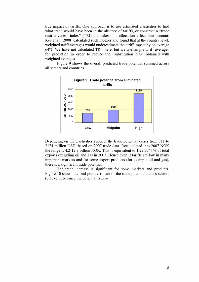
true impact of tariffs. One approach is to use estimated elasticities to find what trade would have been in the absence of tariffs, or construct a “trade restrictiveness index” (TRI) that takes this allocation effect into account. Kee et al. (2008) calculated such indexes and found that at the country level, weighted tariff averages would underestimate the tariff impact by on average 64%. We have not calculated TRIs here, but we use simple tariff averages for prediction in order to reduce the “substitution bias” obtained with weighted averages.
Figure 9 shows the overall predicted trade potential summed across all sectors and countries.
Figure 9: Trade potential from eliminated tariffs
716960
2198
0
500
1000
1500
2000
2500
Low Midpoint High
Mill
ion
2007
USD
Depending on the elasticities applied, the trade potential varies from 711 to 2174 million USD, based on 2007 trade data. Recalculated into 2007 NOK the range is 4.2-12.9 billion NOK. This is equivalent to 1.22-3.74 % of total exports excluding oil and gas in 2007. Hence even if tariffs are low in many important markets and for some export products (for example oil and gas), there is a significant trade potential.
The trade increase is significant for some markets and products. Figure 10 shows the mid-point estimate of the trade potential across sectors (oil excluded since the potential is zero).
19
Figure 10: Trade potential by sector
0 50 100 150 200 250 300 350
Light Industries
Textile
Wood
Transport
Instruments
Food
Metal
Chemicals
Machinery
Fish
Minerals
Million 2007 USD
The trade potential is highest for minerals, fish, machinery and
chemicals. While the latter three were to be expected, the estimate for minerals is more surprising. This is mainly driven by the high elasticity estimate for minerals, which is persistent across specifications in Table 2. The trade potential for minerals is particularly found in the USA and the BRICs.
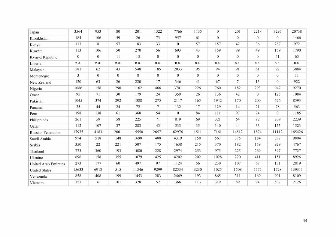
Turning to the export potential by countries, Figure 11 shows the trade potential for the top 20 countries among the 157 included in the analysis. Also here we use the mid-point estimates. Table D1-D3 in the Appendix shows the trade potential (lower, midpoint, upper estimates) by sector and the total, for a list of selected countries. Among these, there are candidates for future FTAs and the tables may be used in order to assess the trade potential from tariff cuts.
20
Figure 11: Trade potential by country, for the top-25
0 20 40 60 80 100 120 140 160 180
Thailand
Venezuela
Italy
Netherlands
Pakistan
Ukraine
Denmark
Saudi Arabia
Turkey
Korea, Rep.
Mexico
Algeria
Canada
France
Nigeria
Sweden
United Kingdom
Japan
Iran, Islamic Rep.
Germany
Brazil
India
China
United States
Russian Federation
Million 2007 USD
Not surprisingly, the BRICs and the USA rank highest, followed by
Germany, Iran and Japan. The figure includes some EU countries due to tariffs for agriculture and particularly fish. The trade potential may however be overestimated since there are tariff-free quotas for fish in the EU so true tariffs are actually lower than according to the TRAINS data (Melchior 2007). The current trade volume is however large with the EU and for that reason the trade potential may be significant even for modest tariff cuts. 6. Non-tariff barriers Tariffs for trade in goods are only one of the numerous elements covered by FTAs and such agreements may cover services, intellectual property rights, investment etc. The European internal market is probably the clearest example showing that the impact of an FTA may extend far beyond that
21
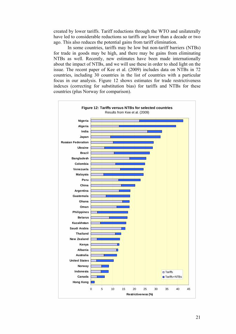
created by lower tariffs. Tariff reductions through the WTO and unilaterally have led to considerable reductions so tariffs are lower than a decade or two ago. This also reduces the potential gains from tariff elimination. In some countries, tariffs may be low but non-tariff barriers (NTBs) for trade in goods may be high, and there may be gains from eliminating NTBs as well. Recently, new estimates have been made internationally about the impact of NTBs, and we will use these in order to shed light on the issue. The recent paper of Kee et al. (2009) includes data on NTBs in 72 countries, including 30 countries in the list of countries with a particular focus in our analysis. Figure 12 shows estimates for trade restrictiveness indexes (correcting for substitution bias) for tariffs and NTBs for these countries (plus Norway for comparison).
Figure 12: Tariffs versus NTBs for selected countriesResults from Kee et al. (2009)
0 5 10 15 20 25 30 35 40 45
Hong Kong
Canada
Indonesia
Norway
United States
Australia
Albania
Kenya
New Zealand
Thailand
Saudi Arabia
Kazakhstan
Belarus
Philippines
Oman
Ghana
Guatemala
Argentina
China
Peru
Malaysia
Venezuela
Colombia
Bangladesh
Brazil
Ukraine
Russian Federation
Japan
India
Algeria
Nigeria
Restrictiveness (%)
TariffsTariffs+NTBs
22
Figure 12 illustrates that for some countries, NTBs constitute the major share of overall barriers in a number of countries. While it is on average (for a lager sample) true that high-tariff countries often also have high NTBs, this relationship is not at all monotonous. Hence one finds low-tariff countries such as the USA, New Zealand and the Philippines that have high NTBs, and one finds higher-taruiff countries such as China and India where the registered magnitude of NTBs is relatively lower. A general precaution should be taken about the data; measuring NTBs is a difficult task and the estimates shown are based on available data. In spite of these data reservations, Figure 12 is sufficient to show that in FTA negotiations, NTBs should be particularly high on the agenda with respect to some countries. 7. Dynamic gains: An ex post assessment of trade predictions for current FTAs The estimates are based on trade and GDP levels in 2007 and therefore static: They do not take into account GDP growth or other changes that may also affect trade. As a check on how such predictions compare to actual trade developments, we will examine how similar predictions would fare, for FTAs that Norway has entered into after 1990. In Table E in the Appendix, we list these agreements, with the year of entry into force and information about tariffs and trade. For these countries, we undertake a simplified calculation of predicted exports five years after the entry into force of the agreement. We then compared this prediction with the actual trade development. For the trade potential estimates, we take into account tariff cuts as well as GDP growth. Table E in the Appendix contains the detailed information. The calculation is simplified for two reasons: For the trade potential, we scale up or down existing trade without taking into account how well it is explained by the gravity regression. In the former results, we compared predicted values from the regressions only. Second, we use nominal trade figures in USD without attempting to find the appropriate deflators, which creates some inaccuracy.
In Figure 13, we show the results for 13 FTA partners. We show the predicted trade potential from tariff elimination and GDP growth along the horizontal axis (with minimum=100), and trade 5 years after the entry into force of the FTA on the vertical axis. In Figure 14, we show a similar graph but with the predicted trade potential from tariff cuts only on the horizontal axis.
23
Figure 13: Trade potential versus real trade increase for 13 FTA partners
Hungary
Poland Mexico
Morocco
Jordan
Croatia
Turkey
Israel
Lithuania
Singapore
Estonia Latvia
Romania
R2 = 0.12060
50
100
150
200
250
300
350
400
100 150 200 250 300 350 400
Trade potential from tariff cuts and GDP growth
Expo
rt in
crea
se a
fter 5
yea
rs
Figure 14: Trade potential versus real trade increase for 13 FTA partners
Romania
LatviaEstonia
Singapore
Lithuania
Israel
Turkey
Croatia
Jordan
Morocco
MexicoPolandHungary
0
50
100
150
200
250
300
350
400
100 120 140 160 180 200 220
Trade potential from tariff cuts
Expo
rt in
crea
se a
fter 5
yea
rs
There is a positive albeit not too impressive association between predictions and actual trade growth, with R2=0.12 for the regression line indicated in Figure 13. In Figure 14, some countries are lined up close to a ray from lower left corner. These are Israel, Latvia, Turkey, Hungary, Poland, Croatia, Jordan and Romania. For these, there is a relatively good proportionality between trade potential and true ex post exports. Singapore, Estonia, Mexico and Morocco are however outliers. GDP growth explains part of the gap, and for Mexico an issue may be that tariffs have not been fully eliminated yet. Figure 13 suggests that the average order of magnitude for predictions is acceptable. For some countries, however, predictions are too high, e.g. Poland and some other countries in Central Europe. In some of
24
these cases, export growth was higher after the first 5-year period and it is hard to say how long time it takes before a trade potential is realised. It is also evident that trade may be affected by a number of aspects beyond those captured by our regression models. For example, security problems and instability may affect trade. For the Palestine Territory, trade remains close to zero in spite of free trade, for obvious reasons, and trade between Norway and Israel has fallen in spite of the FTA. For the majority of Norway’s FTAs there has been fast import growth in spite of modest tariff barriers, in many cases faster than export growth. Even in cases where GDP growth as well as the tariff reduction was larger in the partner country than in Norway, imports into Norway grew faster than exports to the country in question. This indicates that FTAs may have an institutional side which is not captured by our predictions. Furthermore, liberalisation may shift the composition of trade because of comparative advantage, and this is not necessarily captured in gravity-based approaches. Another limitation with static trade predictions is that if initial trade is zero, the prediction for the future will be zero whatever is the scaling. It is easy to find examples of such cases where trade has “taken off”, so the trade increase can be much higher than what we might obtain from static predictions. Russia and Ukraine are examples where trade has expanded rapidly in recent years.
As Russia and Ukraine also illustrate, tariff cuts are also often part of a broader reform process in countries and it can be difficult to establish whether tariffs alone “cause” trade to increase, or if other aspects such as institutional changes and changes in the economic structure is the main driver. Hence if many other variables were to be included in regressions, they could “weaken” the role of tariffs and in some cases even make parameter estimates insignificant. In this paper, we do not try to sort out these more complex interactions between tariffs and other features of the economies of the trade partners.
Hence our gravity model only captures some of the forces driving trade. Static trade predictions provide a tool for examining proportions and sector distribution, but they do not capture all important aspects. These limitations should be kept in mind when interpreting the results. 8. Concluding comments This analysis has shown that even if tariffs facing Norwegian exports have been eliminated or reduced in many markets, there is still a considerable trade potential to be gained from further tariff elimination. Our estimates suggest trade can increase by 1.2-3.9 percent or 4-13 billion NOK; with the largest increases for the exports of minerals, fish, machinery and chemicals. In order to derive these predictions we have estimated the impact of tariffs on trade, using a large dataset for 2007. By trying different estimation models we have shown that there is some uncertainty about the exact magnitude of the elasticity estimates, and we have therefore indicated a range for the trade potential with lower and upper bounds. Using historical data we have shown that gravity-based predictions are correlated with true trade developments, but trade is affected by a number of other aspects that are not taken into account in the analysis.
25
In the analysis, we also observed that the predictive power of gravity regressions tends to shrink over time. The reasons for this constitute an interesting issue for future research. In the analysis, we have also argued that tariff elasticities used to examine FTAs should be different from elasticities related to tariff changes for all imports of a country. We were not fully able to distinguish between the two empirically, but found some evidence supporting this argument empirically. The study has been made within a short period of time and more work could be done in order to refine the econometric approach; for example by controlling for country-level heterogeneity and zero trade flows. In spite of this we believe that the estimates presented provide a useful tool for assessing the potential gains from trade agreements. References Anderson, J.E. and E. van Wincoop, 2003, Gravity with Gravitas: A Solution to the
Border Puzzle, American Economic Review 93(1): 170-92. Baldwin, R. and D. Taglioni, 2006, Gravity for dummies and dummies for gravity
equations, NBER Working Paper 12516. Buch., C.M., J. Kleinert and F. Toubal, 2004, The distance puzzle: on the
interpretation of the distance coefficient in gravity equations, Economics Letters 83: 293-298.
Disdier, A. and K. Head, 2008, The puzzling persistence of the distance effect on bilateral trade, Review of Economics and Statistics 90(1): 37-48.
Feenstra, R.C., J.R. Markusen and A.K. Rose, 2001, Using the gravity equation to differentiate among alternative theories of trade, Canadian Journal of Economics 34(2): 430-447.
Gaulier, G. and S. Zignago, 2008, BACI: A World Database of International Trade at the Product-level. The 1995-2004 Version. Mimeo, July 2008, available at www.cepii.fr.
Hoekman, B. and A. Nicita, 2008, Trade Policy, Trade Costs, and Developing Country Trade. Washington DC: World Bank Policy Research Working Paper No. 4797.
Kee, H.L., A. Nicita and M. Olarreaga, 2009, Estimating Trade Restrictiveness Indexes, The Economic Journal 119: 172-19.
Kee, Nicita, Olarreaga, 2008, Import Demand Elasticities and Trade Distortions, Review of Economics and Statistics 90(4): 666-682.
Linnemann, H., 1966, An econometric study of trade flows, Amsterdam: North-Holland.
Maurseth, Per B., 2003, Norsk utenrikshandel, markedspotensial og handelshindringer. Oslo, NUPI-notat 647.
Melchior, A., 1997, On the economics of market access and international economic integration, University of Oslo, Department of Economics, Dissertations in Economics No.36-197.
Melchior, A., 2006, Tariffs in World Seafood Trade, Rome: FAO Fisheries Circular FIIU/C1016, ISSN 0429-9329.
Melchior, A., 2007, WTO eller EU-medlemskap? Norsk fiskerinæring og EUs handelsregime. Oslo: NUPI Report, May 2007.
26
Appendix A: About data The World Bank and United Nations Conference on Trade and Development (UNCTAD) have developed software for access and retrieval of information on trade and tariffs called the World Integrated Trade Solution (WITS). Using WITS, tariff data were downloaded from the Trade Analysis Information System (TRAINS). TRAINS contain information on 120 countries for 2007, 166 for 2006 and 105 for 2005. It should be noted that most countries do not report tariff data annually - less than half of the countries reported tariff levels for both 2007 and 2008 for instance. Data on the Dominican Republic and Kuwait were downloaded from the WTO Integrated Database (IDB).
In total, tariff data for approximately 150 countries (counting the European Union and its 27 member states as one unit) were downloaded. The data set covers 48 out for the countries listed by the NHD (GCC countries consist of seven member states). The missing countries include Cayman Islands and Liberia. For Serbia, we make an estimate of the trade potential using tariffs for Serbia and Montenegro. The product classification is internationally agreed upon and changes over time so it exists in different “vintages”. Hence some countries present tariffs in the latest version which is the “Harmonised System” of 2007, or HS2007. Tariffs for other countries may however be reported in older classifications; i.e. HS2002, HS1996 or HS1988/932. Furthermore, trade data classification may vary across countries. Hence it is a puzzle to obtain the best possible match between tariffs and trade data.
Tariff data for 130 countries (counting the European Union and its 27 member states as one unit) were used in the regressions, from which 100 were data for 2007, 26 from 2006 and 4 from 2004. 39 of the countries listed by the NHD were included in the regression analysis. Six out of the 130 countries had missing values for preferential tariffs. Tariff data for some countries were defined as too old to be included in the regression analysis, the case of Kazakhstan (2004) and Belarus (2002). Other countries lacked trade data for 2007 and were therefore excluded. Due to missing trade or missing values, the number of countries included in each regression could be lower.
A particular feature of the TRAINS database is that one obtains tariffs only for traded goods. Hence if one asks for average tariffs for imports from Norway and Norway only exports ten out of the 5000 product groups, one obtains an average only for these ten groups. We have used this method for retrieving PRF tariffs, since we are interested in those tariffs that actually apply to the observed exports. For BND, AHS and MFN tariffs at the product level, data are retrieved for imports from the world. In order to make tariff averages across product groups comparable, they should be done for the same selection of products. In the descriptive statistics presented, we therefore use tariffs for goods that are exported by Norway, also for BND, AHS and MFN tariffs. For smaller countries, these averages could therefore be based on rather few products and we do not report such averages in detail since they may be less reliable due to the product selection. For averages at the product level, such averages are broader and more reliable (i.e. as those shown in Figures 4 and 5 in the main text).
Chem Instrument Light Ind Machinery Metal Minerals Textile Transport Wood Food Fish TOTAL Japan 8499 1898 225 556 2632 18832 2815 0 400 5156 11697 52710
Method for calculating trade potential (Figure 13 and Figure 14): - We set Norwegian exports to the country in question the year before entry into force of the agreement at 100, and calculate the development
in the subsequent years. - Second, we obtain from the TRAINS database simple average tariffs for imports from Norway, for goods actually traded in the base year.
We use tariffs for a year preceding but close to the entry into force of the agreement. Some countries are dropped since data are not available. - We undertake a simplified calculation of the trade potential from tariff elimination, using an average of all lower/upper elasticities in Table 2
above, i.e. -4.22. The simplified trade potential is then equal to 100/t-4.22, where t is the average tariff expressed as 1+T/100 (T=% tariff rate). - Fourth, we use data on GDP in current USD and calculate the predicted trade growth from the GDP increase. For this purpose, we use an
average of GDP parameter estimates from Model 6, at 0.955.