Trade Effects on the Personal Distribution of

Wealth ∗

Francesc Obiols-Homs†

Centro de Investigacion Economica, ITAM(This version: October 2003)

Abstract

This paper develops a dynamic Heckscher-Ohlin model and stud-

ies the interaction between international trade and the dynamics of

the wealth distribution in a small open economy. I prove that trade

generates a permanent decline in inequality (relative to the level un-

der autarky) if the economy opens to trade with a stock of capital

sufficiently close to its steady state level. I then use numerical simula-

tions to study wealth distribution dynamics when the economy opens

to trade while far away from the steady state. My results suggest that

trade always helps to reduce inequality in wealth.

Keywords: International Trade, Wealth Distribution

JEL Classification: E21, F11, F17

∗I would like to thank S. Chatterjee, B. Paal, J. Sempere and R. Torres for helpfulcomments and suggestions. All remaining errors are mine.

†Address: ITAM, Av. Camino a Santa Teresa n. 930, Mexico D.F.-10700, Mexico.Tel: 52-55-5628-4197. Fax: 52-55-5628-4058. E-Mail address: obiols@itam.mx

1 Introduction

In the theoretical literature on international trade, the Stolper-Samuelson

theorem stands as one of the main results about income distribution. Roughly

speaking, the theorem states that with the opening to international trade,

prices of relatively abundant factors increase and prices of relatively scarce

factors decrease. This change in factor prices is the consequence of a more

specialized production in goods that use intensively the relatively abundant

factors.1 Thus, the theorem describes the changes in the functional distribu-

tion of income of an economy that opens to international trade.2 However,

it is not obvious how these changes may affect personal inequality in in-

come and/or wealth. Perhaps surprisingly, the effects of international trade

on the personal distribution of wealth have received little attention in the

theoretical literature.

In this paper, I bring together the literatures on optimal paths of capital

accumulation and on inequality, in the context of a small open economy.

Specifically, I extend the study by Chatterjee (1994) of the dynamics of

the distribution of income and wealth in a standard one-sector neoclassical

model of growth to the case of a dynamic Heckscher-Ohlin model of interna-

tional trade similar to that in Atkeson and Kehoe (2000). Chatterjee (1994)

showed that in an economy where agents differ only in their initial wealth,

1There are several empirical applications of the Stolper-Samuelson theorem as an ex-planation for observed wage differentials between skilled and unskilled workers in tradingeconomies. The empirical evidence supporting the theorem is mixed. See, among others,Wood (1997) and Robertson (2001).

2Ripoll (2000) develops a three-good, three-factor, dynamic model and shows that inaddition to relative abundance of factors, the timing of the opening to trade has sizableeffects on steady states and on the dynamic path of factor prices.

1

the transition towards the steady state from below has a negative effect on

the degree of lifetime wealth/income inequality prevailing in the economy.3

His findings are relevant in the study of the effects of international trade

because in a dynamic model, trade is likely to give rise to a different steady

state than under autarky. Following Atkeson and Kehoe (2000), I analyze

the case of a small open-economy that trades intermediate goods with the

rest of the world. In particular, I assume that all economies are identical and

that the only difference among them is that the rest of the world is already

at the steady state. Because of the small open-economy assumption, trade

has no effects on the distribution of wealth in the rest of the world. Nev-

ertheless, the distribution of wealth in the small economy does change over

the transition to the steady state. Over a transition to the steady state from

below (when the initial stock of capital is smaller than its long run level),

these changes in the small open-economy are the result of two conflicting

effects: an “international trade” effect, which tends to reduce inequality in

the functional distribution of income (through the Stolper-Samuelson the-

orem familiar from static models), and a “transition” effect that tends to

increase inequality in the personal distribution of income and wealth.

I state necessary and sufficient conditions for inequality in wealth to fall —

relative to the level under autarky — both at the moment when the economy

opens to international trade, and in the long run. I prove that these condi-

tions are satisfied in several cases. In particular, they are satisfied when the

3Caselli and Ventura (2000) extend these results in a continuous time model withadditional sources of heterogeneity (preferences and labor productivity); see also Sorger(2000) where the effect of a leisure/labor decision is studied. Relatedly, Obiols-Homs andUrrutia (2003) study the dynamics of the distribution of assets.

2

opening to trade occurs once the capital stock of the small open-economy is

sufficiently close to its steady state level under trade. I extend these results

using numerical methods and compare the dynamics of inequality under

trade and under autarky when the economy opens to international trade far

away from the steady state (i.e., starting from arbitrary levels of capital).

I find that inequality in wealth under trade is always smaller than under

autarky. I also find that the sooner the economy opens to international

trade, the smaller will be the level of inequality in the long run. These re-

sults suggest that the “international trade” effect dominates the “transition”

effect.

The intuition to explain the results comes from the Stolper-Samuelson the-

orem. When the small economy opens to international trade, labor is rela-

tively more abundant than in the rest of the world. Since the assumptions

of the Heckscher-Ohlin model are satisfied, the economy then finds it opti-

mal to specialize production in the labor intensive good, thus labor income

increases and capital income decreases. These changes in factor prices ben-

efit more those agents for whom labor income represents a larger fraction of

their wealth portfolio, i.e., agents with relatively fewer units of capital. As

a consequence of trade, therefore, inequality shrinks.

The results in this paper are related to other studies about the relationship

between trade and inequality. For instance, Fisher and Serra (1996) develop

a static model in which the income of the median voter determines whether

an economy opens to free trade or not with other richer/poorer economies.

More related to this paper, Das (2000) studies the effects of trade among

3

similar economies on the personal distribution of income and wealth in an

overlapping generations model where agents live for one period (and there is

a bequest motive), markets are imperfectly competitive, and where capital is

tradable. In my model I relax these assumptions and obtain similar results

to Das. Also, Wynne (2003) follows a different approach and studies how

the distribution of wealth affects the pattern of trade in a model where firms

in different sectors have differential access to credit. In Wynne’s model the

distribution of wealth determines comparative advantages, thus the distri-

bution affects the pattern of trade and trade affects the distribution, and it

is able to explain Trefler’s missing trade mystery. With respect to applied

work, the empirical evidence regarding the effects of international trade on

inequality is inconclusive. For instance, Edwards (1997) reports that trade

reforms do not seem to affect income distribution, Litwin (1998) finds that

trade openness in general worsen income distribution, and Wei and Wu

(2001) find that openness to trade and urban-rural inequality are negatively

associated in Chinese cities. In this respect, my results suggest that to un-

derstand trade effects on personal inequality we need to look at the pattern

of production and specialization.

The paper continues as follows: Section 2 introduces a world with many

competitive economies, section 3 describes equilibrium dynamics under au-

tarky and shows that the results in Chatterjee (1994) can be extended to

two-sector economies. Section 4 studies the effects of trade on the distri-

bution of wealth of a small open-economy. Section 5 extends the previous

results using numerical methods, and section 6 concludes. An appendix

4

at the end of the paper contains proofs and a description of the numerical

methods used in section 5.

2 The model

There is a large number of small economies. These economies are identical

in all respects except perhaps in the initial distribution of capital among

agents. A typical economy is described below. To fix notation, a variable

xit denotes the value of x corresponding to agent i in a period t, and xt

denotes the average over agents. These variables under international trade

are denoted xit, and xt. Long run values under autarky and trade are denoted

respectively x∗ and x∗.

2.1 Production

In each economy production is organized in two sectors, one producing a final

good that can be devoted to consumption and investment, and the other

producing intermediate goods which are used as inputs in the final goods

sector. In the intermediate goods sector there are two industries producing

goods x and y using capital and labor as primary factors. Technologies for

production display constant returns to scale and the only difference between

them is that they use primary inputs in different intensities: x = kθxl1−θx , y =

kηy l1−ηy , with θ, η ∈ (0, 1). In the previous equations the subindices x and y

of the primary factors indicate amounts used in the production of each good.

Assuming θ > η, the production of x is capital intensive. Furthermore, by

5

assuming Cobb-Douglas technologies I am also ruling out factor intensity

reversals. The technology in the final goods sector also displays constant

returns to scale and uses as inputs intermediate goods only: z = xγy1−γ ,

with γ ∈ (0, 1). Finally, in each sector there is a large number of firms andmarkets are perfectly competitive.

2.2 Consumers, preferences, and endowments

Each economy is inhabited by N agents indexed by i = 1, 2, 3, ...N . Each

of these agents behaves so as to maximize the present value of the utility

derived from the consumption of the homogeneous final good over an infinite

horizon:∞Xt=0

βtu(cit), (1)

where β ∈ (0, 1) is the subjective discount factor, which is taken to bethe same for all agents. In the rest of the paper it will be assumed that

preferences take the form of u(cit) = log(cit− c), where c ≥ 0 is a real number

(the same for all agents). If c > 0, the marginal utility of consumption

can be arbitrarily large even for strictly positive levels of consumption. The

interpretation in this case is that there is a minimum consumption level and

it will be required that cit − c ≥ 0. As shown in Chatterjee (1994), the

implications of trade on the personal distribution of wealth I derive in this

paper will also hold under a more general class of utility functions.4

Agents are endowed with ki0 units of productive capital in the first period.

4This class includes u(c) = ρ(c+ ψc)σ with a) σ < 1 but different from zero, ρ = 1/σ,ψ = 1 and c a real number, or b) σ = 2, ρ = −1/2, ψ = −1 and c > 0. It also includesthe case of u(c) = −c exp(−ψc) with both c and ψ strictly positive.

6

The initial endowment of capital is the only difference among agents. To

transfer capital across periods agents have access to the following investment

technology:

kit+1 = iit + (1− δ)kit. (2)

In the previous equation δ ∈ [0, 1] is the depreciation rate of capital. Inaddition to the initial endowment of capital, in the beginning of each period

agents receive one unit of time which they inelastically supply as labor. Both

capital and labor are freely mobile in the intermediate goods sector.

2.3 An agent’s problem

The utility maximization problem a given agent i solves can be written

formally as follows:

maxP∞t=0 β

t log(cit − c)s. to cit + i

it = wt + rtk

it,

kit+1 = iit + (1− δ)kit,

cit ≥ c, kit ≥ 0, ∀t ≥ 0, given ki0,

(3)

where we have used the fact that free mobility of primary factors and perfect

competition in factor markets imply a unique equilibrium rental rate of

capital, rt, and labor, wt. Assuming the initial condition for capital is

large enough so that the solution to the problem is interior, the first-order

7

necessary condition for optimality is given by

1

cit − c= βRt+1

1

cit+1 − c, (4)

where Rt+1 = rt+1+1−δ is the interest factor. Following Chatterjee (1994),let lifetime wealth of agent i in a period t be given by

ωit = Rthkit +Wt

i, (5)

where Wt =P∞j=0(wt+j/(

Qjs=0Rt+s)). Notice that ω

it is composed of the

real value of capital at the end of the period plus the real present value

of labor. This measure of wealth is useful for the purposes of this paper

because it summarizes the changes in factor-prices, which is a central issue

in international trade theory.

The measure of inequality I use is the coefficient of variation (standard

deviation divided by the mean) in ωt. In order to study the dynamics

of inequality it is convenient to substitute repeatedly Equation (4) in the

budget constraint in (3) and use the definition of ωit to obtain:

cit = (1− β)ωit + Pt, (6)

where Pt = cP∞j=0((βRt+1+j − 1)/(

Qjs=0Rt+1+s)). Thus an agent’s con-

sumption is a linear function of wealth, and hence, of capital. From the

budget constraint of the agent and the definition of wealth it is easy to see

that wealth evolves over time according to ωit+1 = Rt+1(ωit − cit). Finally,

using Equation (6) to substitute out consumption in the previous expression

8

we obtain ωit+1 = βRt+1ωit −Rt+1Pt. It follows that

cv(ωt+1) = cv(ωt)ωtωt+1

βRt+1. (7)

Thus equation (7) states that wealth dynamics are determined by the growth

rate of wealth relative to the interest factor. Given that wealth is essentially

a combination of all future prices of capital and labor, the focus of the paper

is on the differences between autarky and international trade with respect

to competitive prices of primary factors.

In the following section I restate the result in Chatterjee (1994) about wealth

dynamics in a closed economy using the coefficient of variation, and later I

turn to the effects of international trade.

3 Wealth dynamics under autarky

The following result establishes that For any of the previous economies, a

competitive equilibrium under autarky is a list of sequences {pxt , pyt , wt, rt}such that markets for primary factors and intermediate goods clear and such

that the aggregation of optimal decisions of agents satisfy market clearing

for final goods. The following result establishes that this market clearing

condition can be written as in the one-sector neoclassical growth model.

Lemma 1. Let νt and lt denote the fractions of capital and labor, respectively,

devoted to the production of good x. Under the maintained assumptions,

νt = ν∗ and lt = l∗, thus they are independent of kt. Market clearing for the

9

final goods can be written as:

PN c

it + k

it+1

N= Akξt + (1− δ)

PN k

it

N, (8)

where ξ = θγ + η(1− γ) and A = (ν∗/l∗)θγ³1−ν∗1−l∗

´η(1−γ)l∗γ(1− l∗)1−γ .

Proof: See the Appendix.

Remember that consumption in Equation (6) is linear in wealth, and wealth

in Equation (5) is linear in capital. It follows from the market clearing

equation (8) that average capital depends only on the consumption of an

agent that has the average capital in the economy. Therefore the evolution

of capital over time can be studied by means of the problem of a central

authority that solves

maxP∞t=0 β

t log(ct − c)s. to ct + kt+1 = Ak

ξt + (1− δ)kt

ct ≥ c, kt ≥ 0, ∀t ≥ 0, given k0.(9)

This problem is a version of the neoclassical model of growth studied at

length in the literature. Since c can be positive I will assume that the initial

stock of capital is larger than some lower bound k ≥ 0 so that the feasibleset is not empty. I will also assume that k < k∗.5 The following proposition

states some well known properties of the solution to the previous problem

(see theorem 1 in Obiols-Homs and Urrutia (2003) for a proof). For future

5If c ≤ 0, then k = 0. For c > 0 the feasible set will be empty unless there exists asolution to Akξ − c− δk = 0. I will assume that the previous equation has two solutionsan that the smaller one satisfies k < k∗, where k∗ is the unique k satisfying condition (i)in Proposition 1.

10

reference, the theorem introduces a version of the welfare theorems to state

the connection between the optimal allocation and competitive factor prices.

Proposition 1. Under the maintained assumptions, if k0 > k then there

exists a sequence {ct, kt+1} that solves the planner’s problem. The sequence{ct, kt+1} monotonically converges to stationary values {c∗, k∗} satisfying(i) Aξ(k∗)ξ−1 − δ = (1 − β)/β, and (ii) c∗ = A(k∗)ξ − δk∗. Furthermore,

Rt = Aξkξ−1t + 1− δ and wt = A(1− ξ)kξt for all t.

I will refer to a situation where k0 < k∗ —and thus the stock of capital will

be growing over time— as a transition from below. We are now ready to

describe wealth dynamics:

Proposition 2 (Chatterjee 1994). Over a transition from below under au-

tarky: a) inequality monotonically increases over time if c > 0; and b)

inequality remains constant over time if c = 0.

Proof: From ωt+1 = Rt+1(ωt− ct), Equation (6), and the definition of ωt weobtain

ωtωt+1

βRt+1 = 1 +Pt

kt+1 +Wt+1.

Next, kt < k∗ implies that βRt > 1 for all t. For the first part, use the

previous result together with c > 0 to get that Pt > 0 for all t. It follows

that βRt+1ωt+1/ωt > 1, for all t. The desired conclusion is obtained using

this observation in Equation (7). The second part follows directly from the

same reasoning because with c = 0, then Pt = 0 for all t.

In the following section I study the implications of the previous proposition

once the economies engage in international trade in intermediate goods.

11

4 Wealth dynamics in a small open-economy

Following Atkeson and Kehoe (2000), I study the effects of trade on the dis-

tribution of lifetime wealth of a small economy that starts its development

process once the rest of the world has reached the steady state. In particular

I assume that all but one economy started growing towards the steady state

at the same time and with the same level of initial capital. This means that

whether these economies were allowed to trade in intermediate goods over

the transition to the steady state is of no consequence. Therefore the equi-

librium dynamics for these economies are described by Propositions 1 and

2 above: all economies converge to the same steady state independently of

the initial distribution of wealth, and at the steady state the only difference

among them is in the stationary distribution of wealth.

Consider now the equilibrium dynamics of the economy that starts its pro-

cess of development once the rest of the world has reached the steady state.

This economy is allowed to trade intermediate goods at the international

equilibrium prices. Since aggregate dynamics do not depend on the initial

distribution of wealth, the evolution of this economy can be described by

the decisions of a central authority that buys and sells intermediate goods

in international markets and that organizes efficiently domestic production.

As in the preceding section, it is useful to write the problem in per capita

terms so that the planner chooses the fraction of available capital and labor

to be devoted to the production of each intermediate good. Using the nota-

tion introduced above the problem of the central authority can be described

as

12

maxP∞t=τ β

t log(ct − c)s. to ct + kt+1 = (xdt )

γ(ydt )1−γ + (1− δ)kt

xst = (νtkt)θ l1−θt , yst = ((1− νt)kt)

η(1− lt)1−η,p∗xxdt + p∗yydt = p∗xxst + p∗yyst ,

ct ≥ c, kt ≥ 0, lt ∈ [0, 1], νt ∈ [0, 1] ∀t ≥ τ,

given kτ .

(10)

The first equation is the feasibility constraint that restricts consumption

and capital accumulation to the sum of current output and undepreciated

capital; the second and third equations simply relate the domestic supply

of intermediate goods to the technology constraints; the forth equation is

the condition for balance in international trade. The following Proposition

3 collects a number of useful results about the solution of the previous

planner’s problem (the proof is omitted because the arguments in Atkeson

and Kehoe (2000), given in a model with continuous time, apply without

change to the present context).

Proposition 3 (Atkeson and Kehoe 2000). Let τ denote the period when the

late-bloomer opens to international trade. There exist

ky =(1− θ)η

θ(1− η)

Ãp∗xp∗y

µθ

η

¶θ µ1− θ

1− η

¶1−θ!1/(η−θ),

with 0 < ky < k∗ such that: a) if kτ < ky, then νt = 0 = lt ∀t ≥ τ and k is

monotonically increasing and converges to k∗ = ky; and b) if ky ≤ kτ ≤ k∗,then νt = ν, lt = l (with ν ∈ [0, ν∗] and l ∈ [0, l∗]), and kt = kτ = k∗ ∀t ≥ τ .

13

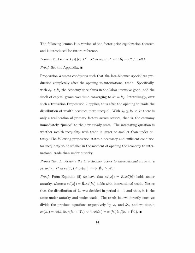
The following lemma is a version of the factor-price equalization theorem

and is introduced for future reference.

Lemma 2. Assume kt ∈ [ky, k∗]. Then wt = w∗ and Rt = R∗ for all t.

Proof: See the Appendix.

Proposition 3 states conditions such that the late-bloomer specializes pro-

duction completely after the opening to international trade. Specifically,

with kτ < ky the economy specializes in the labor intensive good, and the

stock of capital grows over time converging to k∗ = ky. Interestingly, over

such a transition Proposition 2 applies, thus after the opening to trade the

distribution of wealth becomes more unequal. With ky ≤ kτ < k∗ there isonly a reallocation of primary factors across sectors, that is, the economy

immediately “jumps” to the new steady state. The interesting question is

whether wealth inequality with trade is larger or smaller than under au-

tarky. The following proposition states a necessary and sufficient condition

for inequality to be smaller in the moment of opening the economy to inter-

national trade than under autarky.

Proposition 4. Assume the late-bloomer opens to international trade in a

period τ . Then cv(ωτ ) ≤ cv(ωτ ) ⇐⇒ Wτ ≥Wτ .

Proof: From Equation (5) we have that sd(ωiτ ) = Rτsd(kiτ ) holds under

autarky, whereas sd(ωiτ ) = Rτsd(kiτ ) holds with international trade. Notice

that the distribution of kτ was decided in period t − 1 and thus, it is thesame under autarky and under trade. The result follows directly once we

divide the previous equations respectively by ωτ and ωτ , and we obtain

cv(ωτ ) = cv(kτ )kτ/(kτ +Wτ ) and cv(ωτ ) = cv(kτ )kτ/(kτ + Wτ ).

14

The intuition for Proposition 4 is as follows. Since labor income is the same

for all agents, an increase in its present value benefits more those agents

for whom labor income represents a larger fraction of their lifetime wealth.

Thus wealth inequality necessarily declines if the present value of labor in-

come increases with trade. This latter condition is a dynamic version of the

Stolper-Samuelson theorem about the functional distribution of income that

holds in static Heckscher-Ohlin models: trade promotes gains in efficiency

by specializing production in goods that use intensively relatively abundant

factors, and as a consequence, income rewarding those factors tends to in-

crease and the income rewarding relatively scarce factors tends to decrease.

The next result collects two situations where the previous condition is sat-

isfied. In those situations the same condition is also sufficient to provide a

decline in inequality in all future periods after the opening to trade.

Corollary 1. Assume the late-bloomer opens to international trade in a pe-

riod τ . International trade promotes a permanent reduction in wealth in-

equality when: a) ky ≤ kτ < k∗; or b) kτ < ky, and c = 0, δ = 1.

Proof: To see part a), notice that since kτ < k∗, then Proposition 2a im-

plies inequality will increase under autarky. Furthermore, Proposition 1

implies that wt is monotonically increasing and converges to w∗, and that

Rt is monotonically decreasing and converges to R∗. Under trade, how-

ever, the economy jumps to a steady state where wt = w∗ and Rt = R∗,

∀τ ≥ t (by Lemma 2). Therefore Wτ > Wτ and Proposition 4 implies

that cv(ωτ ) < cv(ωτ ). This completes the argument because cv(ωτ+j) =

cv(ωτ ) < cv(ωτ ) ≤ cv(ωτ+j) for all j > 0. To see part b), notice that

15

Proposition 3 implies that the planner’s problem with trade can be written

without loss of generality as

maxP∞t=τ β

t log(ct − c)s. to ct + kt+1 = A(kt)ξ + (1− δ)kt

ct ≥ c, kt ≥ 0, ∀t ≥ τ, given kτ ,

(11)

where ξ = η and A = A³1−l∗1−ν∗

´η (1−γ)(1−l∗)(k

∗)γ(θ−η). It is well known that

with c = 0 and δ = 1, then kt+1 = βAξkξt and kt+1 = βAξkξt for all

t ≥ τ . It is straight forward to check that Wτ = kτ (1 − ξ)/(ξ(1 − β)) and

Wτ = kτ (1−ξ)/(ξ(1−β)). Thus Wτ > Wτ because ξ = η < γθ+(1−γ)η = ξ.

Therefore the result follows from Propositions 2b and 4.

The previous corollary states that when there is no transition, either because

kτ ≥ ky and thus the stock of capital does not change over time, or becauseδ = 1 and c = 0 in which case the distribution of wealth remains constant

over time, the distribution of wealth improves with the opening to interna-

tional trade. When kτ < ky and c > 0 the late-bloomer observes a transition

towards the new steady state with trade. Over this transition there will be

the “international trade” effect discussed after Proposition 4, and the “tran-

sition” effect described in Proposition 2. These two effects work in opposite

directions. In particular, even though capital is the relatively scarce factor

in the late-bloomer economy, agents that own an amount of capital larger

(smaller) than the average capital will observe a larger (smaller) increase in

their lifetime wealth over the transition to the new steady state with trade.

Is it possible that the long run level of inequality with international trade

16

is larger than the level it would have prevailed had the economy remained

closed? Proposition 5 below states necessary and sufficient conditions for the

long run level of inequality under trade to be smaller than under autarky.

Proposition 5. Assume c > 0 and that the late-bloomer opens to inter-

national trade in a period τ with kτ < k∗. Then cv(ω∗) < cv(ω∗) ⇐⇒Rτu

0(cτ )/(ω∗u0(c∗)) < Rτu0(cτ )/(ω∗u0(c∗)).

Proof: The proof proceeds in two steps. In the first step, we write

cv(ω∗) = cv(kτ )kτk∗

k∗

k∗ +W ∗βRτu0(cτ )u0(c∗)

, (12)

and a similar expression for cv(ω∗). The previous expression follows from the

fact that cv(ω∗) = cv(k∗)k∗/(k∗+W ∗), and that from the budget constraint

in period τ , together with the expression for consumption in Equation (6)

and the definition of ωτ we get that kiτ+1 = βRτkiτ + wτ − (1− β)RτWτ −

Pτ . Therefore cv(kτ+1) = cv(kτ )kτ/kτ+1βRτ , and iterating forward, we

get that cv(k∗) = cv(kτ )kτ/k∗ limj→∞

Qj−1s=0(βRτ+s). Next, use the first

order condition for optimality in the consumer’s problem in (4) to get that

limj→∞Qj−1s=0(βRτ+s) = βRτu

0(cτ )/u0(c∗). The expression in (12) is the

result of combining the previous equations. Moreover, the present value of

labor income (W ∗) is the same under both trade and autarky because of

Lemma 2. Likewise, the term cv(kτ )kτ is also the same under trade and

autarky because it was determined in period τ − 1. For the second step,

17

define

Λ(kτ ) ≡ cv(kτ )kτβÃ

Rτ

k∗ +W ∗u0(cτ )u0(c∗)

− Rτ

k∗ +W ∗u0(cτ )u0(c∗)

!.

The function Λ(kτ ) measures the difference in the long run level of inequality

between trade and autarky as a function of the stock of capital in the moment

of the opening to international trade. The conclusion follows multiplying

Λ(kτ ) by R∗ and dividing the terms in parenthesis by R∗ and R∗ (which are

identical by Lemma 2).

The last result in this section uses Proposition 5 to state that there is an

open set of levels of capital smaller than k∗ such that if the economy opens

to trade with a capital level in that set, then inequality in the long run is

smaller than under autarky.

Corollary 2. Assume c > 0 and that the late-bloomer opens to international

trade in a period τ with kτ < k∗ but close to k∗. Then cv(ω∗) < cv(ω∗).

Proof: Part a) of Corollary 1 implies that Λ(k∗) < 0. This concludes the

proof, since Λ(k) is continuous for kτ > k.

It is difficult to generalize the result of the previous corollary for capital

levels arbitrarily far away from the steady state. Intuitively, in the class of

economies studied in this paper the changes in the distribution of wealth are

directly related to the speed of convergence to the steady state through the

changes in factor prices. Then, a neoclassical economy converges faster to its

steady state the further away it is from it. This suggests that convergence

under autarky should be faster than under trade because k∗ < k∗. However,

18

convergence is also faster the smaller is the capital share in the technology to

produce final goods (see King and Rebelo (1993)). Since ξ < ξ, this suggests

a faster convergence under trade than under autarky. In the following section

I resort to numerical simulations to investigate these issues.

5 Simulations

I simulate several examples of the evolution of inequality for the late-bloomer

economy under autarky and under trade.6 The parameter values used in the

benchmark simulations are as follows. I use β = .99 and δ = .025 which are

commonly used in applied work for the U.S. economy simulating quarterly

data. For the parameters in the technologies I use γ = .5, θ = .38 and

η = .34. These parameter values produce a capital share about .36 which is

again standard in the quantitative literature. I also assume c = 0.1, and I fix

an arbitrary distribution of capital which then implies the initial distribution

of wealth. The distribution of capital under autarky in the opening period

τ is used to determine the initial distribution of wealth under trade.

Figure 1 displays the evolution of inequality in lifetime wealth over the tran-

sition to the steady state for an economy under autarky. It also displays

the evolution of inequality under trade starting with a capital level about

90% of that at the steady state. As predicted by Proposition 2, inequality

is clearly increasing over the transition under both regimes. However, in-

equality initially falls after the opening to international trade, then it starts

6A brief description of the numerical method used to solve the model can be found inthe Appendix.

19

increasing and it converges to a lower level than it would under autarky.

This transition can be seen as an example where both Corollaries 1 and 2

hold. Furthermore, in this example inequality under trade is smaller than

under autarky in all periods over the transition to the steady state.

Figure 2 displays the evolution of inequality under autarky and under trade

for the economy opening with a stock of capital equal to 10% and 50% of

the stock of capital at the steady state with trade. The figure suggests that

the result in Corollary 2 applies even with a capital level very far away from

the level at the steady state with trade. Furthermore, it is clear from Figure

2 that the later the opening to international trade occurs, the smaller the

reduction in inequality relative to that under autarky will be and the larger

will be in the long run. I have obtained the same sort of results under sev-

eral initial distributions of wealth, minimum consumption requirements, and

different combinations for the parameter values in the technologies (these

results are not reported for reasons of space). These experiments suggest

that the “international trade” effect from the Stopler-Samuelson theorem al-

ways dominates the “transition” effect, thus trade effectively helps to reduce

wealth inequality.

6 Conclusion

In this paper I develop a dynamic Heckscher-Ohlin model to study interna-

tional trade effects on personal wealth inequality in a small open economy.

Over a transition to the steady state from below inequality in wealth tends

20

to increase. This effect due to the transition may be counterbalanced once

the economy opens to international trade because the Stolper-Samuelson

theorem holds and thus income accruing to relatively abundant factors in-

creases and income accruing to relatively scarce factors decreases. I formally

show that international trade promotes a decline in wealth inequality when

the economy opens to trade with a level of capital sufficiently large (i.e.,

close to the steady state level with trade). I then use numerical simulations

to investigate the effects of international trade starting from arbitrary initial

levels of capital. In the simulations I find that trade always helps reduce

inequality in wealth relative to the level of inequality under autarky.

My results suggest that the effect of trade in factor prices dominates the

effect of the transition and therefore, the changes in the personal distribu-

tion of wealth are directly related to changes in the functional distribution

of income. Like in the static Heckscher-Ohlin model, the changes in the

functional distribution of income in the dynamic model are linked to the

pattern of trade. This observation should be useful in empirical work trying

to asses the effects of international trade on personal inequality. Finally, it

would be interesting to investigate the predictions of a similar model but

abandoning the small open-economy assumption. This extension is left for

future work.

21

References

Acemoglu, D. and J. Ventura, 2001. The World Income Distribution.

NBER Working Paper 8083.

Atkeson, A. and P.J. Kehoe, 2000. Paths of Development for Early-

and Late-Bloomers in a Dynamic Heckscher-Ohlin Model. Staff Report 256,

Fed of Minneapolis.

Caselli, F., and J. Ventura, 2000. A Representative Consumer Theory

of Distribution. The American Economic Review, Vol. 90, pgs. 909-26.

Chatterjee, S., 1994. Transitional Dynamics and the Distribution of

Wealth in a Neoclassical Growth Model. Journal of Public Economics, Vol.

54, pgs. 97-119.

Das, S.P., 2000. Trade among Similar Countries and the Personal Distri-

bution of Income and Wealth. Economica, Vol. 67, pgs. 265-81.

Edwards, S., 1997. Trade Policy, Growth, and Income Distribution. The

American Economic Review, Vol. 87, pgs. 205-210.

Fischer, R.D. and P. Serra, 1996. Income Inequality and Choice of

Free Trade in a Model of Intraindustry Trade. The Quarterly Journal of

Economics, pgs. 41-64.

King, R.G. and S.T. Rebelo, 1993. Transitional Dynamics and Eco-

nomic Growth in the Neoclassical Model. American Economic Review, Vol.

83, pgs. 908-31.

Litwin, C., 1998. Trade and Income distribution in Developing Countries.

22

Working Papers in Economics n. 9, Goteborg University.

Obiols-Homs, F., and C. Urrutia 2003. Transitional Dynamics and

the Distribution of Assets. Economic Theory, forthcoming.

Ripoll, M., 2000. Paths of Development and Income Distribution in the

Global Economy. Working Paper, University of Rochester.

Robertson, R., 2000. Relative Prices and Wage Inequality: Evidence

from Mexico. Working Paper, Macalester College.

Samuelson, P.A., 1996. International Factor-Price Equalisation Once

Again. Chapter 1 in International Trade: Selected Readings, edited by J.

Bhagwati, the MIT Press.

Sorger, G., 2000. Income and Wealth Distribution in a Simple Model of

Growth. Economic Theory, Vol. 16, pgs. 23-42.

Wei, S. and Y. Wu, 2001. Globalization and Inequality: Evidence from

Within China. NBER Working Paper 8611.

Wood, A., 1997. Openness and Wage Inequality in Developing Countries:

The Latin American Challenge to East Asian Conventional Wisdom. The

World Bank Economic Review, Vol. 11, n. 1.

Wynne, J., 2003. Wealth as a Determinant of Comparative Advantage.

Working Paper, Duke University.

23

Appendix

Proofs

Proof of Lemma 1: Since both intermediate goods are fundamental in the

production of the final good, in equilibrium they will be produced in all peri-

ods. It follows from the profit maximizing problem of final goods producers

that

px,tpy,t

=γ

1− γ

ytxt. (13)

The stock of capital in per capita terms used in the production of each

intermediate good can be written as kx,t = νtkt and ky,t = (1 − νt)kt.

Since primary factors are perfectly mobile across firms and industries, in

equilibrium it must be the case that wx,t = wy,t and that rx,t = ry,t. Using

Equation (13) in the equilibrium condition rx,t = rt,y, and using the fact

that in equilibrium factor prices coincide with the value of their marginal

productivity, a few manipulations produce η/θ(1− γ)/γ = (1− νt)/νt, thus

ν∗ = θγ/(η(1− γ) + θγ). Using the fact that prices of primary factors are

the same in both industries and dividing the FOC of intermediate goods

produces provides θ/(1 − θ)lxt /ν∗ = η/(1 − η)(1 − lxt )/(1 − ν∗), thus l∗ =

(1− θ)γ/((1− η)(1− γ)+ (1− θ)γ). The market clearing condition for final

goods stated in the text is obtained after substituting the expressions for l∗

and ν∗ intoPN (c

it + k

it+1)/N = xγt y

1−γt + (1− δ)

PN k

it/N .

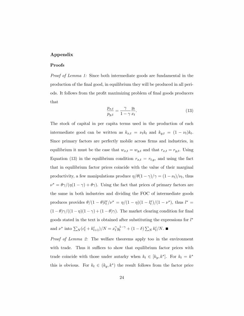
Proof of Lemma 2: The welfare theorems apply too in the environment

with trade. Thus it suffices to show that equilibrium factor prices with

trade coincide with those under autarky when kt ∈ [ky, k∗]. For kt = k∗

this is obvious. For kt ∈ (ky, k∗) the result follows from the factor price

24

equalization theorem (see for instance Samuelson (1996)), since in both the

late-bloomer and the rest of the world goods prices are the same, there is no

perfect specialization, technologies are the same in all economies, and they

do not allow factor intensity reversals. For kt = ky, notice that when the

late-bloomer specializes completely in the production of y the correspond-

ing first order condition implies that r = p∗yηkη−1y . For the early-bloomers

the corresponding expression is given by r = p∗yη(k∗(1− ν∗)/(1− l∗))η−1.Since early-bloomers produce both intermediate goods, at the steady state

p∗x/p∗y = γ/(1−γ)Bk∗η−θ, where B = ((1−ν∗)/(1− l∗))η(l∗/ν∗)θ(1− l∗)/l∗.Using the definitions for l∗, ν∗ and ky, it follows that ky = k∗(1−ν∗)/(1−l∗).Therefore the factor price equalization theorem also applies to the limiting

case of kt = ky.

Computation

The numerical method is based on dynamic programming: starting from an

arbitrary function v0 of the state k for the value function, perform iterations

on:

1

Akξ + (1− δ)k − k0 − c = βv00(k).

The equation above is the first order condition associated to the correspond-

ing planner’s problem, and it is evaluated on a grid of points. The decision

rule for capital accumulation is approximated with piecewise linear func-

tions between grid points (see Obiols-Homs and Urrutia (2003) for further

details).7 Once the decision rule for capital has approximately converged I

7In practice I use 1,300 evenly spaced points in the grid. Computing time is smallbecause there is only one state variable.

25

simulate a transition of capital and factor prices towards the steady state

over 1,000 periods and I compute the objects of interest. To gain accuracy

in the computations, I first compute lifetime wealth of the representative

agent over the transition. Then I fix an initial distribution of capital and I

simulate the transition of 10 agents as follows. From Equation (6) it follows

that cit = ct + (1− β)Rt(kit − kt), and kit+1 is determined using the budget

constraint of each agent. The same Equation (6) implies that

ωit = ωt +cit − ct1− β

.

Using the ωit’s to compute the coefficient of variation at each period is much

more accurate than using the recursive expression in Equation (7).

26

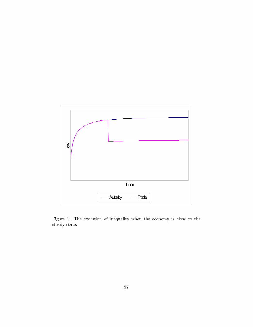
Time

cv

Autarky Trade

Figure 1: The evolution of inequality when the economy is close to thesteady state.

27

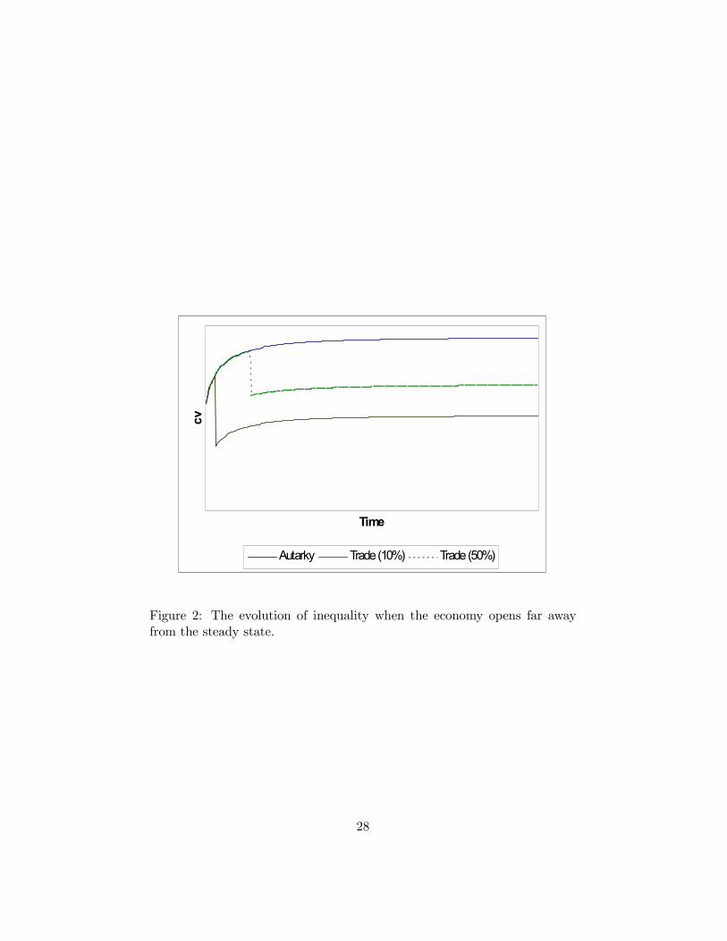
Time

cv

Autarky Trade (10%) Trade (50%)

Figure 2: The evolution of inequality when the economy opens far awayfrom the steady state.

28