46
WP/14/52 Trade Integration and Business Cycle Synchronization: A Reappraisal with Focus on Asia Romain Duval, Kevin Cheng, Kum Hwa Oh, Richa Saraf and Dulani Seneviratne

WP/14/52
Trade Integration and Business Cycle Synchronization: A Reappraisal with Focus on
Asia
Romain Duval, Kevin Cheng, Kum Hwa Oh, Richa Saraf
and Dulani Seneviratne
© 2014 International Monetary Fund WP/14/52
IMF Working Paper
Asia and Pacific Department
Trade Integration and Business Cycle Synchronization: A Reappraisal with Focus on Asia
Prepared by Romain Duval, Kevin Cheng, Kum Hwa Oh, Richa Saraf
and Dulani Seneviratne
Authorized for distribution by Romain Duval
April 2014
Abstract
This paper reexamines the relationship between trade integration and business cycle synchronization (BCS) using new value-added trade data for 63 advanced and emerging economies during 1995–2012. In a panel framework, we identify a strong positive impact of trade intensity on BCS—conditional on various controls, global common shocks and country-pair heterogeneity—that is absent when gross trade data are used. That effect is bigger in crisis times, pointing to trade as an important crisis propagation mechanism. Bilateral intra-industry trade and trade specialization correlation also appear to increase co-movement, indicating that not only the intensity but also the type of trade matters. Finally, we show that dependence on Chinese final demand in value-added terms amplifies the international spillovers and synchronizing impact of growth shocks in China.
JEL Classification Numbers: E32; F42
Keywords: Trade, Value Added, Business Cycle Synchronization, Spillovers, Asia.
Author’s E-Mail Address: [email protected]; [email protected]; [email protected]; [email protected]; [email protected]
This Working Paper should not be reported as representing the views of the IMF. The views expressed in this Working Paper are those of the author(s) and do not necessarily represent those of the IMF or IMF policy. Working Papers describe research in progress by the author(s) and are published to elicit comments and to further debate.

2
Contents Page
I. Introduction ............................................................................................................................3
II. Stylized Facts about Business Cycle Synchronization ..........................................................5 A. Properties of Business Cycle Synchronization in Asia .............................................5 B. The Role of Global, Regional and Sub-regional Factors ..........................................7
III. The Role of Trade in Driving BCS ....................................................................................11 A. A Bird’s Eye View of the Literature .......................................................................11 B. Methodology ...........................................................................................................12 C. Results .....................................................................................................................21 D. Interpretation ...........................................................................................................25 E. An Additional Model: Assessing China Spillovers .................................................26
IV. Concluding Remarks and Policy Implications ..................................................................28
References ................................................................................................................................30 Appendixes I. Further Details about the Dynamic Factor Analysis ............................................................33 II. Further Details on the Data .................................................................................................40 III. Robustness for Econometrics—Using Four Periods .........................................................45

3
I. INTRODUCTION
Over the past two decades, trade integration has increased rapidly within the world economy, and particularly so within Asia. Gross trade in volume terms rose at an average rate of 8 percent per annum during 1990–2012, twice the average pace outside Asia. In valued-added terms, trade increased at an average annual growth rate of over 10 percent during the same period, also double the average pace outside Asia. Not only have Asian economies traded more with one another, they have also traded differently, becoming more vertically integrated as a tight-knit supply-chain network across the region was formed. Have changes in trade patterns, in particular greater trade integration, led economies to move more in lockstep, and disproportionately so within Asia? Theoretically, the answer to that question is a priori ambiguous, and empirically the evidence seems to be weaker than initially thought. The relationship between trade integration and business cycle synchronization (BCS) has been subject to extensive research, motivated in good part by the optimum currency area literature (OCA) that was pioneered by Mundell (1961) and McKinnon (1963) and given new impetus by Frankel and Rose (1997, 1998). A wide range of empirical papers (e.g., Frankel and Rose, 1997, 1998; Baxter and Kouparitsas, 2005; Imbs, 2004; Inklaar and others, 2008), including in an Asian context (e.g., Kumakura, 2006; Park and Shin, 2009), have found that trade intensity increases synchronization, although the magnitude of the impact varies across studies. However, while existing studies have relied on a variety of approaches including cross-section, pooled and simultaneous equation techniques, and paid a good deal of attention to endogeneity issues, they have typically not accounted for fixed country-pair factors and common global shocks. Yet, as stressed by Kalemli-Ozcan, Papaioannou and Peydro (2013), controlling for both is required to address omitted variable bias and thereby identify a causal link. Indeed they and Abiad and others (2013) find the relationship between trade integration and BCS to be insignificant, and that between financial integration and BCS to change sign relative to a cross-section regression, when such controls are added in a panel setup. Earlier studies that accounted for country-pair heterogeneity also found weaker or no effects of overall trade intensity on BCS (Calderon, Chong and Stein, 2007; Shin and Wang, 2004), although they found the type of trade to matter. The present paper contributes to the literature on trade integration and BCS in several ways. First, we account systematically for country-pair heterogeneity and common global shocks throughout the analysis. Second, and crucially, we depart from all existing studies by using value added instead of gross trade data, building on the recent joint OECD-WTO initiative on trade in value added. As indicated for instance by Unteroberdoerster and others (2011), and as will be illustrated below, gross trade data misrepresent trade linkages across countries amid increasingly important supply-chain networks across the globe. Using value-added trade data instead will prove crucial to identifying a robust impact of trade on BCS. Third, this paper goes beyond bilateral trade intensity and explores the BCS impact of the nature of trade and specialization, including vertical integration, trade specialization correlation, and

4
intra-industry trade, while also controlling for other influences on BCS such as financial integration (including bank, FDI, portfolio flows) and macro-economic policy synchronization across countries. Finally, in separate but related analysis, we also examine the impact of a China shock on other economies and whether and how this shock is propagated through various trade channels. The main findings from this paper are the following:
Consistent with results from other recent studies, BCS appears to spike across the globe during crises. Based on the quasi-correlation indicator proposed by Abiad and others (2013), output correlations outside of Asia peaked during the 2008/09 Global Financial Crisis (GFC), while within Asia the biggest spikes in BCS occurred during the Asian Crisis of the late 1990s. During normal times, BCS is typically much lower but has nonetheless been on an upward trend over the past two decades, particularly in Asia.
Based on a dynamic factor analysis, global factors appear to be playing a major role in driving business cycles in Asia and elsewhere.
Using a sample of 63 advanced and emerging economies spanning the last two decades, a macro panel analysis based on value-added trade data finds that bilateral trade intensity has a significant, positive, and robust effect on bilateral BCS among country pairs. Significant, though smaller effects of intra-industry trade and correlation of trade specialization are also found.
The impact of trade integration on BCS is greater in crisis times than in normal times, that is, trade amplifies the synchronizing impact of common shocks. This is qualitatively consistent with the concomitant finding—already featured in —that financial integration increases BCS in crisis times, even though it typically reduces it during normal times.
Growth spillovers from China—a growing source of BCS, especially within Asia—are significant, sizeable, and larger in economies that are more dependent on final demand from China in value-added terms.
The remainder of the paper proceeds as follows: Section II presents some stylized facts about BCS, with particular focus on Asia, including results of a factor analysis on the roles played by global, regional, and sub-regional factors. Section III explores the role of the intensity and nature of trade for BCS while also covering effects of financial integration. It also features additional, related analysis of the spillovers of growth shocks in China to other economies. Section IV concludes.

5
II. STYLIZED FACTS ABOUT BUSINESS CYCLE SYNCHRONIZATION
A. Properties of Business Cycle Synchronization in Asia
Measurement Throughout this paper, our default measurement of BCS is the instantaneous quasi-correlation measure proposed by Abiad and others (2013):
∗ ∗ ∗
∗
where is the quasi-correlation of real GDP growth rates of country i and j in year t,
denotes the output growth rate of country i in year t and; ∗and represent the mean and standard deviation of output growth rate of country i, respectively, during the sample period. The growth rate is measured as the first difference of the log of real GDP. This measure has advantages over methods commonly used by similar studies because: First, this enables the calculation of co-movement at every point in time rather than
over an interval of time. By contrast, most of the literature measures output co-movement between two economies by the rolling Pearson correlation of actual or detrended growth rates between a country pair over a window period. This artificially introduces autocorrelation of the BCS time series due to a high degree overlapping observations throughout the sample. In addition, given that this paper uses annual data over the past two decades,1 the rolling correlation measure would likely be dominated by outliers during the Asian crisis and the GFC.
Second, the quasi-correlation measure retains some nice statistical properties. First, it can be easily shown that the period mean of the measure would asymptotically converge to the standard Pearson correlation coefficient. Second, at any point in time, the measure is not necessarily bounded between -1 and 1. As argued by Otto and others (2001) and Inklaar and others (2008), if the BCS measure lies between -1 and 1, the error terms in the regression explaining it are unlikely to be normally distributed.2
1 We are using annual data because most of the (value added) trade variables are available at the annual or lower frequency. We also focus on the past two decades because data on many relevant variables were not available earlier for many emerging economies.
2 Consequently, these authors transformed the dependent BCS variable so that it is not bounded between -1 and 1.

6
Finally, we calculate correlations based on actual rather than detrended growth rates, because the latter crucially depend on the choice of filtering methods and we use low-frequency data anyway (annual data over two decades).
BCS developments Using annual data for 63 countries, including 34 advanced economies (7 of which in Asia) and 29 emerging economies (8 of which in Asia), developments of BCS in Asia and elsewhere since 1990 are depicted in Figure 1: Consistent with findings from other similar studies, BCS sharply increased in crisis
times. The largest spikes occurred around the GFC outside Asia, and around the Asian crisis of the late 1990s within Asia (Top left panel).
During normal times, BCS has been much smaller but also shown some upward trend since the 1990s around the globe, including in Asia. That increase in BCS has been particularly large in Asia and Latin America, although BCS within both regions was still considerably lower than within the euro area during the 2000s. Within Asia, BCS appears to be particularly high among ASEAN-5 economies, which include Indonesia, Malaysia, the Philippines, Singapore, Thailand (Top right panel). Similar results are obtained using the standard Pearson correlation coefficients (Bottom left panel).
China’s output co-movements vis-à-vis the rest of the Asia have increased, but Asian economies continue to co-move more with Japan and the United States (bottom right panel). This likely reflects the continued importance of global factors in driving business cycles across the region, as examined below.

7
Figure 1
B. The Role of Global, Regional and Sub-regional Factors
Setup Before assessing the role of observable drivers of BCS such as trade and financial linkages using regression analysis, we employ a dynamic factor model to analyze the roles played by unobservable global, regional, sub-regional, and country factors in explaining the evolutions of business cycles.
Following the approach of Hirata, Kose, and Otrok (2013), our model is constructed as follows: 3
, ~ 0, . . . . . . , . ~ 0, .
Here, stands for a vector comprising growth rates of GDP, consumption, and investment; . stands for factors; and represents residuals. Each factor and residuals are assumed to
3 Details of the estimation are discussed in Appendix I.
-1
0
1
2
3
4
5
6
7
8
9
-0.5
0.0
0.5
1.0
1.5
2.0
2.5
3.0
3.5
4.019
95
1996
1997
1998
1999
2000
2001
2002
2003
2004
2005
2006
2007
2008
2009
2010
2011
2012
Intra-Asia
China supply-chain economies
Full sample
ASEAN-5
Median Instantaneous Quasi-correlations by Region
Sources: IMF, World Economic Outlook; and IMF staff calculations.Note: China supply-chain economies include China, Korea, Malaysia, the Philippines, Taiwan Province of China, and Thailand. They are identified based on the intensity of their trade linkages (in value added terms).
-0.10.00.10.20.30.40.50.60.70.8
Intra-Asia ASEAN-5 China supply-chain
Intra-EA 11 Intra-LATAM Full sample
Instantaneous Quasi-Correlations by Region(Excludes crisis periods)
1990s 2000s
Sources: IMF, World Economic Outlook; and IMF staff calculations.Note: China supply-chain economies include China, Korea, Malaysia, the Philippines, Taiwan Province of China, and Thailand. They are identified based on the intensity of their trade linkages (in value added terms). Euro Area includes the 11 countries that adopted the euro in 1999.
-0.2-0.10.00.10.20.30.40.50.60.70.8
Intra-Asia ASEAN-5 China supply-chain
Intra-EA 11 Intra-LATAM Full sample
1990s2000s
Sources: IMF, World Economic Outlook; and IMF staff calculations.Note: China supply-chain economies include China, Korea, Malaysia, the Philippines, Taiwan Province of China, and Thailand. They are identified based on the intensity of their trade linkages (in value added terms). Euro Area includes the 11 countries that adopted the euro in 1999.
Bilateral Pearson Growth Correlations by Region(Excludes crisis periods)
-0.30
-0.10
0.10
0.30
0.50
0.70
ASEA
N-5
Rest
of A
sia
Full
sam
ple
ASEA
N-5
Rest
of A
sia
Full
sam
ple
ASEA
N-5
Rest
of A
sia
Full
sam
ple
ASEA
N-5
Rest
of A
sia
Full
sam
ple
China Japan United States Euro Area
1990-99 2000-12
Average Bilateral Pearson Correlations
Sources: IMF, World Economic Outlook; and IMF staff calculations.
8
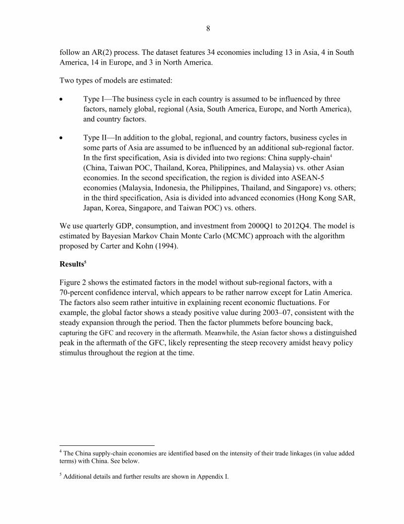
follow an AR(2) process. The dataset features 34 economies including 13 in Asia, 4 in South America, 14 in Europe, and 3 in North America.
Two types of models are estimated:
Type I—The business cycle in each country is assumed to be influenced by three factors, namely global, regional (Asia, South America, Europe, and North America), and country factors.
Type II—In addition to the global, regional, and country factors, business cycles in some parts of Asia are assumed to be influenced by an additional sub-regional factor. In the first specification, Asia is divided into two regions: China supply-chain4 (China, Taiwan POC, Thailand, Korea, Philippines, and Malaysia) vs. other Asian economies. In the second specification, the region is divided into ASEAN-5 economies (Malaysia, Indonesia, the Philippines, Thailand, and Singapore) vs. others; in the third specification, Asia is divided into advanced economies (Hong Kong SAR, Japan, Korea, Singapore, and Taiwan POC) vs. others.
We use quarterly GDP, consumption, and investment from 2000Q1 to 2012Q4. The model is estimated by Bayesian Markov Chain Monte Carlo (MCMC) approach with the algorithm proposed by Carter and Kohn (1994).
Results5
Figure 2 shows the estimated factors in the model without sub-regional factors, with a 70-percent confidence interval, which appears to be rather narrow except for Latin America. The factors also seem rather intuitive in explaining recent economic fluctuations. For example, the global factor shows a steady positive value during 2003–07, consistent with the steady expansion through the period. Then the factor plummets before bouncing back, capturing the GFC and recovery in the aftermath. Meanwhile, the Asian factor shows a distinguished peak in the aftermath of the GFC, likely representing the steep recovery amidst heavy policy stimulus throughout the region at the time.
4 The China supply-chain economies are identified based on the intensity of their trade linkages (in value added terms) with China. See below.
5 Additional details and further results are shown in Appendix I.

9
Figure 2
-7.0
-6.0
-5.0
-4.0
-3.0
-2.0
-1.0
0.0
1.0
2.0
2000 2001 2002 2003 2004 2005 2006 2007 2008 2009 2010 2011 2012
Global Factor(Median and 15 and 85-percent percentiles, models without sub-regional factors)
Source: IMF staff estimates.
-4.0-3.0-2.0-1.00.01.02.03.04.05.06.07.0
2000 2001 2002 2003 2004 2005 2006 2007 2008 2009 2010 2011 2012
Regional Factor: Asia(Median and 15 and 85-percent percentiles, models without sub-regional factors)
Source: IMF staff estimates.
-3.0
-2.0
-1.0
0.0
1.0
2.0
3.0
4.0
2000 2001 2002 2003 2004 2005 2006 2007 2008 2009 2010 2011 2012
Regional Factor: Latin America(Median and 15 and 85-percent percentiles, models without sub-regional factors)
Source: IMF staff estimates.
-4.0
-3.0
-2.0
-1.0
0.0
1.0
2.0
3.0
2000 2001 2002 2003 2004 2005 2006 2007 2008 2009 2010 2011 2012
Regional Factor: Europe(Median and 15 and 85-percent percentiles, models without sub-regional factors)
Source: IMF staff estimates.
-3.0
-2.0
-1.0
0.0
1.0
2.0
3.0
2000 2001 2002 2003 2004 2005 2006 2007 2008 2009 2010 2011 2012
Regional Factor: North America(Median and 15 and 85-percent percentiles, models without sub-regional factors)
Source: IMF staff estimates.

10
Next, given that factors are orthogonal to each other in the model, we can calculate the contribution of each factor to the total variance by decomposing the variance as follows.
Figure 3, upper panel shows the role of each factor in driving business cycles under the Type I model. Specifically, the global factor explains on average about 35 percent of output fluctuations in individual economies.6 The contribution of the global factor is lower in Asia than in North America and in Europe, but it is nonetheless larger that of the regional or country factors. Based on these results, there appears to be no evidence that Asia has been decoupling from the rest of the world over the last two decades. In other words, the region remains more globalized than regionalized.
Figure 3, lower panel shows similar results under the Type II model, which incorporates sub-regional factors. While this addition does not seem to alter the big picture, a couple of intuitive findings emerge regarding the role of global factors across various parts of Asia. In particular, global factors are found to explain a greater share of business cycle fluctuations among those countries that are part of the China supply-chain than within the rest of Asia, consistent with the view that the China supply-chain economies are comparatively more integrated with the world economy and thereby more sensitive to its fluctuations. Similarly, the global factor has higher explanatory power in advanced Asian economies than in emerging Asia, in line with the fact that the former are more deeply integrated than the latter in the global economy.
6 For simplicity and focus, we mainly focus here on results for output even though the model includes consumption and investment.
Figure 3
0.0
0.1
0.2
0.3
0.4
0.5
0.6
Asia South America Europe North America
Global Regional Country
Source: IMF staff estimates.Note: Based on simple averages of contributions across the economies featured in each region.
Output Variance Decomposition by Region: Type I: Three–layer Model
0.0
0.1
0.2
0.3
0.4
China supply-chain
Non-China supply-chain
ASEAN-5 non-ASEAN-5 Advanced Asia Emerging Asia
Global Regional Subregional Country
Source: IMF staff estimates.Note: Based on simple averages of contributions across the economies featured in each region. China supply-chain economies include China, Korea, Malaysia, the Philippines, Taiwan Province of China, and Thailand. They are identified based on the intensity of their trade linkages (in value added terms).
Output Variance Decomposition by Region: Type II: Four–layer Model

11
III. THE ROLE OF TRADE IN DRIVING BCS
A. A Bird’s Eye View of the Literature
In this section we begin by reviewing very briefly what economic theory postulates and what existing empirical research finds about the BCS impact of trade integration, as well as of financial integration and policy coordination whose effects will also be examined below.
Trade integration Theoretically, the impact of trade on BCS is ambiguous: On the one hand, according to traditional trade theory, openness to trade should lead
to a greater specialization across countries. To the extent this holds in practice, and insofar as business cycles are dominated by industry-specific supply shocks, higher trade integration should reduce BCS.
On the other hand, if the patterns of specialization and trade are dominated by intra-industry trade, greater trade integration should be associated with a higher degree of output co-movement in the presence of industry-specific supply shocks. If instead demand factors are the principal drivers of business cycles, greater trade integration should also increase BCS, regardless of whether the patterns of specialization are dominated by inter- or intra-industry trade.
Given the ambiguity of the theory, the impact of trade integration on BCS is essentially an empirical question. And indeed this has been a heavily researched area, with cross-sectional regression and simultaneous equation approaches essentially finding a significant positive impact—with some disagreement regarding its magnitude—and most recent panel regression work controlling for country-pair fixed effects and common global shocks essentially finding no effect (see above). Financial integration Theoretically, financial integration, like trade integration, has an ambiguous impact on BCS:7 On the one hand, Morgan and others (2004) developed a model in which if firms in
one country are hit by negative shocks to the value of their collateral or productivity, then in a more financially integrated world domestic and foreign banks would decrease lending to this country and reallocate the funds to another, thereby causing cycles to further diverge. Likewise, in the workhorse international real business cycle (RBC) model of Backus, Kehoe and Kydland (1992), capital will leave a country hit by a negative productivity shock and get reallocated elsewhere under complete
7 For greater details, see Kalemli-Ozcan and others (2013).
12
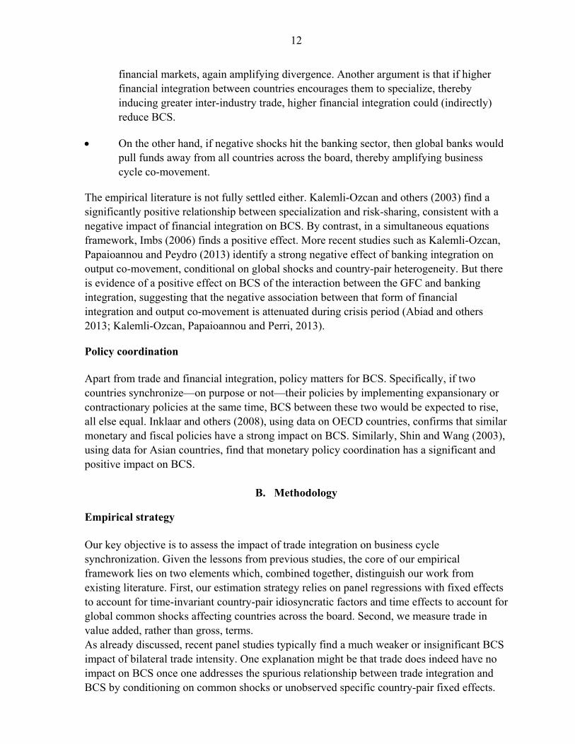
financial markets, again amplifying divergence. Another argument is that if higher financial integration between countries encourages them to specialize, thereby inducing greater inter-industry trade, higher financial integration could (indirectly) reduce BCS.
On the other hand, if negative shocks hit the banking sector, then global banks would pull funds away from all countries across the board, thereby amplifying business cycle co-movement.
The empirical literature is not fully settled either. Kalemli-Ozcan and others (2003) find a significantly positive relationship between specialization and risk-sharing, consistent with a negative impact of financial integration on BCS. By contrast, in a simultaneous equations framework, Imbs (2006) finds a positive effect. More recent studies such as Kalemli-Ozcan, Papaioannou and Peydro (2013) identify a strong negative effect of banking integration on output co-movement, conditional on global shocks and country-pair heterogeneity. But there is evidence of a positive effect on BCS of the interaction between the GFC and banking integration, suggesting that the negative association between that form of financial integration and output co-movement is attenuated during crisis period (Abiad and others 2013; Kalemli-Ozcan, Papaioannou and Perri, 2013).
Policy coordination Apart from trade and financial integration, policy matters for BCS. Specifically, if two countries synchronize—on purpose or not—their policies by implementing expansionary or contractionary policies at the same time, BCS between these two would be expected to rise, all else equal. Inklaar and others (2008), using data on OECD countries, confirms that similar monetary and fiscal policies have a strong impact on BCS. Similarly, Shin and Wang (2003), using data for Asian countries, find that monetary policy coordination has a significant and positive impact on BCS.
B. Methodology
Empirical strategy Our key objective is to assess the impact of trade integration on business cycle synchronization. Given the lessons from previous studies, the core of our empirical framework lies on two elements which, combined together, distinguish our work from existing literature. First, our estimation strategy relies on panel regressions with fixed effects to account for time-invariant country-pair idiosyncratic factors and time effects to account for global common shocks affecting countries across the board. Second, we measure trade in value added, rather than gross, terms. As already discussed, recent panel studies typically find a much weaker or insignificant BCS impact of bilateral trade intensity. One explanation might be that trade does indeed have no impact on BCS once one addresses the spurious relationship between trade integration and BCS by conditioning on common shocks or unobserved specific country-pair fixed effects.

13
However, another explanation might simply be that gross trade data used in recent—and indeed all—studies fail to capture properly true underlying trade linkages and interdependence across countries in a world characterized by a rapid increase in the fragmentation of production processes and a growing share of vertical trade. For example, as shown by Xing and Detert (2010) in the case of iPhone trade, in 2009 China’s value added only accounted for 3.6 percent of total trade with the United States, with the rest of the value added being reaped by Germany, Japan, Korea, the United States and other countries via their exports to China. In this case, using gross bilateral trade data vastly overstates China’s trade dependence vis-à-vis the United States, while understating other countries’ trade dependence on the U.S. trade––which is mostly indirect, via exports to China of components that are then assembled and re-exported by China to the United States (and other) markets. In order to correct for this potentially serious measurement issue, we essentially use value-added trade data throughout this paper. Furthermore, as shown in some previous studies, not only is bilateral trade intensity important, but so are patterns of trade and specialization. Accordingly, in addition to trade intensity, we explore the BCS effects of vertical versus horizontal integration, intra-industry versus inter-industry trade, and the correlation of specialization across country pairs. While this paper is not the first one to do so, to the best of our knowledge, it is the first to compute and test for the impact of trade in value-added terms. Data8 We begin with four trade variables: trade intensity, vertical integration, intra-industry trade, and bilateral correlation of specialization. Table 1 depicts the within correlation of the trade variables with each other. Since the magnitude of within correlation of the various trade variables is low, we will be able to introduce them in our model simultaneously without running into multi-collinearity issues.
8 For a more detailed discussion of how various data and indicators are computed, see Appendix II.
14
Note: The within correlations between two variables xijt and yijt are calculated as the correlation between ( ,
. . .. ) and ( ,. . ..), where, . ∑ , . ∑ and ..
∗∑ ∗ epresentsacountrypair.
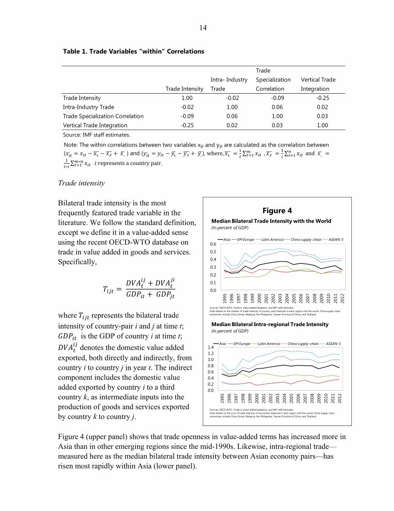
Trade intensity Bilateral trade intensity is the most frequently featured trade variable in the literature. We follow the standard definition, except we define it in a value-added sense using the recent OECD-WTO database on trade in value added in goods and services. Specifically,
where represents the bilateral trade
intensity of country-pair i and j at time t; is the GDP of country i at time t;
denotes the domestic value added exported, both directly and indirectly, from country i to country j in year t. The indirect component includes the domestic value added exported by country i to a third country k, as intermediate inputs into the production of goods and services exported by country k to country j. Figure 4 (upper panel) shows that trade openness in value-added terms has increased more in Asia than in other emerging regions since the mid-1990s. Likewise, intra-regional trade—measured here as the median bilateral trade intensity between Asian economy pairs—has risen most rapidly within Asia (lower panel).
Table 1. Trade Variables "within" Correlations
Trade Intensity Intra- Industry Trade
Trade Specialization Correlation
Vertical Trade Integration
Trade Intensity 1.00 -0.02 -0.09 -0.25Intra-Industry Trade -0.02 1.00 0.06 0.02Trade Specialization Correlation -0.09 0.06 1.00 0.03Vertical Trade Integration -0.25 0.02 0.03 1.00Source: IMF staff estimates.
Figure 4
0.0
0.1
0.2
0.3
0.4
0.5
0.6
1995
1996
1997
1998
1999
2000
2001
2002
2003
2004
2005
2006
2007
2008
2009
2010
2011
2012
Asia EM Europe Latin America China supply-chain ASEAN-5
Median Bilateral Trade Intensity with the World(In percent of GDP)
Sources: OECD-WTO, Trade in Value Added database; and IMF staff estimates. Note: Based on the median of trade intensity of country pairs featured in each region with the world. China supply-chain economies include China, Korea, Malaysia, the Philippines, Taiwan Province of China, and Thailand.
0.00.20.40.60.81.01.21.4
1995
1996
1997
1998
1999
2000
2001
2002
2003
2004
2005
2006
2007
2008
2009
2010
2011
2012
Asia EM Europe Latin America China supply-chain ASEAN-5
Median Bilateral Intra-regional Trade Intensity(In percent of GDP)
Sources: OECD-WTO, Trade in Value Added database; and IMF staff estimates. Note: Based on the sum of trade intensity of economies featured in each region with the world. China supply-chain economies include China, Korea, Malaysia, the Philippines, Taiwan Province of China, and Thailand.

15
Vertical integration The next trade variable is the vertical trade integration between two countries. A priori, vertical trade could have a specific impact on BCS over and above that of trade intensity (for supportive empirical evidence using country industry-level data, see di Giovanni and Levchenko, 2010). For instance, limited or inexistent short-term substitutability of inputs could propagate shocks along a vertical supply chain in the event of disruptions in parts of it, as was evident in Asia in the wake of the earthquake and tsunami in Japan in 2011. In regression analysis we measure vertical integration between two countries by the extent to which one country’s exports in value- added terms rely on intermediate inputs from the other country. Like trade intensity, we also define it bilaterally:9
where denotes the vertical trade integration between countries i and j; represents
the share in country i’s exports that is attributable to the (foreign) value-added content coming from country j. Figure 5 decomposes the value of total gross exports into its domestic and foreign value-added components for various countries and regions. It shows that the share of foreign value added embedded in total exports has generally increased in Asia economies, particularly in China and in East Asia reflecting the “China supply-chain” network. However, the extent of vertical integration varies across the region: specifically, as displayed in Figure 6, value added coming from or going to China has increased across Asian economies, while that coming from or going to Japan has declined. Within ASEAN-5, vertical integration with ASEAN-5 partners
9 Note that vertical trade intensity could alternatively be defined as the ratio of (the sums of each country’s) foreign value added to (the sums of) GDP, in line with the definition of trade intensity above. However, the trade and vertical trade intensity variables would then be collinear and could not be included simultaneously in the regressions. For this reason, controlling for trade intensity, we instead assess any additional effect of vertical (versus non-vertical) trade through a variable that is the ratio of (the sums of) foreign value added to (the sums of) domestic value added. That said, alternative vertical trade variables were tried in the regressions, without any of them turning out to be statistically significant and robust.
1022
13 13 714 12
34 3039
27 28
9078
87 87 9386 88
66 7061
73 72
0102030405060708090
100
1995 2012 est.
1995 2012 est.
1995 2012 est.
1995 2012 est.
1995 2012 est.
1995 2012 est.
IND AUS, NZL JPN CHN East Asia (excl. CHN)
ASEAN-5 region
Domestic value added Foreign value added
Figure 5. Domestic and Foreign Value Added Embedded in Exports (In percent of total gross exports)
Sources: OECD-WTO, Trade in Value Added database; and IMF staff estimates.

16
Figure 6
0
5
10
15
20
25
30
351995 2012 est.
China(In percent of total foreign value added embedded in each economy's total exports)
Sources: OECD-WTO, Trade in Value Added database; and IMF staff estimates.
05
1015202530354045
1995 2012 est.
China(In percent of total domestic value added exported by each economy)
Sources: OECD-WTO, Trade in Value Added database; and IMF staff estimates.
0
5
10
15
20
25
30
351995 2012 est.
Japan(In percent of total foreign value added embedded in each economy's total exports)
Sources: OECD-WTO Trade in Value Added database; and IMF staff estimates.
0
5
10
15
20
25
301995 2012 est.
Japan(In percent of total domestic value added exported by each economy)
Sources: OECD-WTO, Trade in Value Added database; and IMF staff estimates.
02468
101214161820
Philippines Indonesia Thailand Malaysia Singapore ASEAN5
1995 2012 est.
ASEAN–5(In percent of total foreign value added embedded in each economy's total exports)
Sources: OECD-WTO, Trade in Value Added database; and IMF staff estimates.
0
5
10
15
20
25
30
Indonesia Malaysia Philippines Thailand Singapore ASEAN-5
1995 2012 est.
ASEAN–5(In percent of total domestic value added exported by each economy)
Sources: OECD-WTO ,Trade in Value Added database; and IMF staff estimates.

17
has also generally increased. Figure 7 suggests that nature of integration with partners differs between China and Japan, with China specializing in downstream activities (e.g., assembling) and Japan specializing in upstream activities (providing various inputs).10 Finally, Figure 8 suggests that the United States and the European Union remain the largest final consumers of Asia’s supply chain, although the importance of final demand coming from China has increased rapidly over the past two decades. Intra-industry Trade Our third trade variable is intra-industry trade between countries. A positive coefficient on this variable would suggest that industry-specific supply shocks are an important source of business cycles fluctuations. Conceptually, intra-industry trade differs from vertical trade since it should reflect two-way trade in similar (finished or intermediate) goods, while vertical trade typically involves trade in different as many parts and components along the supply chain belong to different industries and are therefore subject to different industry-specific shocks. This justifies the inclusion of both the vertical trade integration index and the intra-industry trade measure as separate drivers of BCS in the regressions, all the more so as their (within) correlations are low in practice (see Table 1).
10 Upstream vertical integration with China is defined as foreign value added embedded in country i’s exports that comes from China. Downstream vertical integration with China is defined as foreign value added embedded in China’s exports that come from country i. Both upstream and downstream vertical integration indicators are computed as a percent of country i’s GDP.
Figure 7
0.00.51.01.52.02.53.03.54.04.5
90s 00s 90s 00s 90s 00s 90s 00s
Asia ASEAN-5 Rest of Asia non-Asia
Upstream vertical integration Downstream vertical integration
Median Vertical Trade with China(In percent of GDP)
Sources: OECD-WTO, Trade in Value Added database; and IMF staff estimates. Note: Calculated as period medians of the median country pair. Upstream vertical integration of China is defined as Chinese foreign valueadded content of country j’s exports; and downstream vertical integration is defined as the country j’s foreign value added content of China’s exports.
0.00.51.01.52.02.53.03.54.04.55.0
90s 00s 90s 00s 90s 00s 90s 00s
Asia ASEAN-5 Rest of Asia non-Asia
Upstream vertical integration Downstream vertical integration
Median Vertical Trade with Japan(In percent of GDP)
Sources: OECD-WTO, Trade in Value added database; and IMF staff estimates. Note: Calculated as period medians of the median country pair. Upstream vertical integration of Japan is defined as Japanese foreign value added content of country j’s exports; and downstream vertical integration is defined as the country j’s foreign value added content of Japan's exports.
418
2 8 514
715 10
173
103
92
114
104 8
1 7 8 13
25
16
17 70
018
8
19 7 158
159
17 1016
14 26 14
11 610 3
12 6
107
66
11
9 5
5
76
8 711 10 8 10
6
66
1015 13
5 5
9 6
14 11
1513
30 21 27
24
2319
2920 25
18 23 16 3122
1914 23
15
1816
1817
17 13
2320
2019
20
25
17
18
17
20 20
1721
18
2518 19
17
21
2131
23
2426
0
10
20
30
40
50
60
70
80
90
100
95
Late
st
95
Late
st
95
Late
st
95
Late
st
95
Late
st
95
Late
st
95
Late
st
95
Late
st
95
Late
st
95
Late
st
95
Late
st
95
Late
st
95
Late
st
AUS NZL JPN CHN KOR TWN MYS THA PHL IDN SGP IND HKG
China Japan ASEAN5 US EU Other
Figure 8. Value Added Exported to Partner Countries for Final Demand(In percent of total value added exported for final demand by the country)
Sources: OECD-WTO ,Trade in Value Added database; and IMF staff estimates.

18
Formally, bilateral intra-industry trade can be measured by the Grubel and Lloyd (1975) index, , for a country pair i-j in year t:
1∑ , ,
∑ , ,
where , ( , ) are the exports from (imports to) country i to (from) country j in industry h. The higher the index value, the greater the share of intra-industry trade relative to inter-industry trade between the two countries. It is well-known that the Grubel-Lloyd index is sensitive to the granularity of the trade classification. Regressions were run using alternative Standard International Trade Classifications (SITC), at the three- or five-digit level and for all goods or manufacturing goods only. Results were very consistent and robust across these alternative measures. In light of this, we only show those using the SITC three-digit classification, which is also the one used to compute the trade specialization correlation index described further below. Figure 9 shows that intra-industry trade has moderately increased in Asia, while only slightly increased elsewhere. Trade specialization correlation Lastly, we consider the trade specialization correlation of a country pair. The measure, which comes from UNCTAD, looks at the similarity of the basket of goods the two countries trade with the world. This measure effectively captures the importance of pure industry-specific shocks as it does not require any bilateral trade to take place between the partner countries. A significant positive coefficient on this variable would imply that countries engaging in similar trade, regardless of whether they trade with each other, would tend to co-move owing to industry-specific shocks. Formally, the measure is defined as:
∑ , , , ,
∑ , , , ,
such that , , , , ,
0.00
0.05
0.10
0.15
0.20
0.25
0.30
0.35
Asia non-Asia
1990s 2000s
Figure 9. Degree of Intra-Industry Trade (Median Bilateral Grubel-Lloyd Index; ranges from 0 to 1 )
Sources: United Nations, COMTRADE database; and IMF staff estimates. Note: Calculated as period medians of the median country pairs in each group .
19
where represents the trade specialization correlation between countries i and j in year
t, , denotes the trade specialization index of country i for year t in industry h, , is
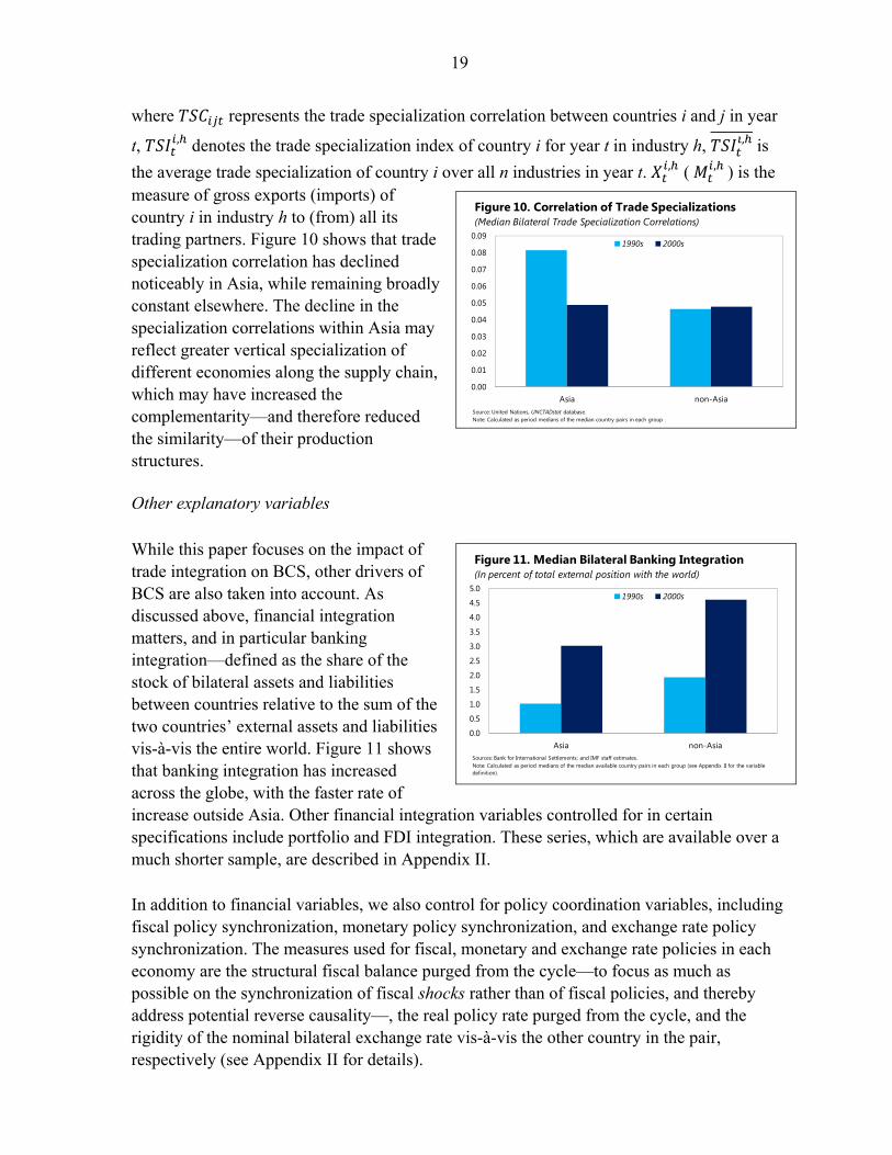
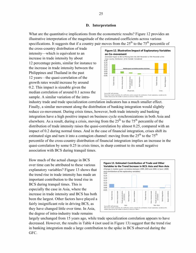
the average trade specialization of country i over all n industries in year t. , ( , ) is the measure of gross exports (imports) of country i in industry h to (from) all its trading partners. Figure 10 shows that trade specialization correlation has declined noticeably in Asia, while remaining broadly constant elsewhere. The decline in the specialization correlations within Asia may reflect greater vertical specialization of different economies along the supply chain, which may have increased the complementarity—and therefore reduced the similarity—of their production structures. Other explanatory variables While this paper focuses on the impact of trade integration on BCS, other drivers of BCS are also taken into account. As discussed above, financial integration matters, and in particular banking integration—defined as the share of the stock of bilateral assets and liabilities between countries relative to the sum of the two countries’ external assets and liabilities vis-à-vis the entire world. Figure 11 shows that banking integration has increased across the globe, with the faster rate of increase outside Asia. Other financial integration variables controlled for in certain specifications include portfolio and FDI integration. These series, which are available over a much shorter sample, are described in Appendix II. In addition to financial variables, we also control for policy coordination variables, including fiscal policy synchronization, monetary policy synchronization, and exchange rate policy synchronization. The measures used for fiscal, monetary and exchange rate policies in each economy are the structural fiscal balance purged from the cycle—to focus as much as possible on the synchronization of fiscal shocks rather than of fiscal policies, and thereby address potential reverse causality—, the real policy rate purged from the cycle, and the rigidity of the nominal bilateral exchange rate vis-à-vis the other country in the pair, respectively (see Appendix II for details).
0.00
0.01
0.02
0.03
0.04
0.05
0.06
0.07
0.08
0.09
Asia non-Asia
1990s 2000s
Figure 10. Correlation of Trade Specializations(Median Bilateral Trade Specialization Correlations)
Source: United Nations, UNCTADstat database.Note: Calculated as period medians of the median country pairs in each group .
0.0
0.5
1.0
1.5
2.0
2.5
3.0
3.5
4.0
4.5
5.0
Asia non-Asia
1990s 2000s
Figure 11. Median Bilateral Banking Integration(In percent of total external position with the world)
Sources: Bank for International Settlements; and IMF staff estimates. Note: Calculated as period medians of the median available country pairs in each group (see Appendix II for the variable definition).

20
The main model We begin with a baseline model that focuses exclusively on the impact of trade and specialization on BCS:
(1)
where is the instantaneous quasi-correlation (as defined in the previous section)
between country-pair i and j at time t; is the country-pair fixed effect, which accounts for
fixed factors such as gravity-type variables or other unobservable time-invariant idiosyncratic factors specific to country-pair i and j; is a time effect, which accounts for time-varying common factors affecting all countries. TRADE captures the four trade and specialization variables mentioned previously—namely trade intensity, vertical integration, intra-industry trade, and trade specialization correlation. Once we estimate the baseline model, in order to check the robustness of the trade variables, we augment the baseline model by adding controls for financial integration and policy synchronization among partner countries:
, , (2)
where FINANCE includes (all or some of the) financial integration variable and POLICY includes policy synchronization variables. Endogeneity Endogeneity is a standard concern in this type of regression. Specifically, trade might be endogenous in the sense that BCS may be driven by some omitted or unobservable variables that are correlated with trade; or there might be reverse causality as higher BCS may induce greater trade intensity between more synchronized countries. In this context, OLS would be both inconsistent and biased. We address this concern in three ways. First, the inclusion of country-pair fixed effects addresses endogeneity problems insofar as omitted variables or the transmission mechanism through which BCS affects trade are time-invariant, such as, for example, geographical proximity, culture, etc. Second, the use of lagged trade intensity variables in an annual panel should further mitigate reverse causality.11 Third, following most studies, we also resort to instrumental variables for both trade intensity and vertical integration. Specifically, for trade intensity, we use a set of time-varying gravity variables, comprising (see Appendix II for 11 Given that intra-industry trade and trade specialization correlation are more structural in nature and less susceptible to reverse causality, their contemporaneous values are used.

21
details): i) the product of the real GDP of the two countries; ii) a WTO membership dummy; iii) the degree of trade cooperation between countries; iv) a geographical distance index; and v) the average import tariff of the two countries. For vertical trade integration, in addition to the five variables above, we add as instruments the average import tariff on intermediate goods—which should correlate negatively with the bilateral intensity of intermediate goods trade—and the difference in real per capita GDP levels between the two countries—which empirically correlates well with the share of intermediate goods in their bilateral trade, as vertical integration tends to exploit factor proportion/price differences across countries, with the China supply-chain providing a typical illustration.
C. Results
Baseline regressions—Trade only Table 2 presents the results of our baseline model with trade variables only (i.e., Equation 1). Due to the presence of serial correlation, standard errors are clustered at country-pair level in all models (including subsequent tables), to allow for autocorrelation and arbitrary heteroskedasticity for each pair (Kalemli-Ozcan, Papaioannou and Peydro, 2013). In order to illustrate the importance of using value-added trade data rather than gross trade data, column 1 of Table 2 shows that trade intensity in gross terms is not significant in explaining co-movement of business cycles once country-pair and time-fixed effects are accounted for. By contrast, column 2 shows that trade intensity in value-added terms has a highly significant and positive effect on BCS. While we do not report below any other regressions including gross trade data, these consistently show an insignificant coefficient, in contrast with the significant and robust impact of value-added trade. Column 3 shows the instrumental variable regression for the model in column 2, confirming that trade intensity is significant and positive. Somewhat surprisingly—insofar as any reverse causality would be expected to be such that higher BCS increases trade intensity— but consistent with findings in earlier studies, the instrumented regressions yield a higher coefficient estimate than do OLS regressions. In column 4, intra-industry trade and trade specialization correlation measures are added, and both have the expected positive coefficients, with statistical significance at 1 the percent level. This also holds true in column 5 when trade intensity is instrumented.

22
However, we fail to find a robust specific impact of vertical trade integration over and above that of trade intensity. As shown in column 6, when the vertical trade integration measure is added, the former three trade variables continue to be positive and significant, but vertical integration enters negatively. However, the latter finding is not robust across alternative specifications, for example, it becomes positive and significant when we remove time fixed effects from the model while all other trade variables in the model keep their sign and significance, or it changes sign when we instrument trade intensity and vertical integration, in ways that depend on the instruments used (results not shown, available upon request).12 Therefore we discard this variable in the remainder of the paper and leave this issue for future work. For instance, it could well be that vertical integration creates co-movement only by propagating up and down the international supply chain only specific shocks such as natural disasters (in the presence of limited short-term substitutability of intermediate inputs used in production processes). This may have been the case for instance with the earthquake and tsunami that affected Japan in 2011, which adversely affected the industrial output of Japan’s downstream trade partners in the regional supply chain. Recent IMF work (IMF,
12 We also do not report alternative regressions using alternative definitions for the vertical trade variable; none of these turned out to show statistically significant and robust effects.
Table 2. Business Cycle Synchronization and Trade Integration
OLS OLS IV OLS IV OLS
(1) (2) (3) (4) (5) (6)
Trade Intensity (Gross) 0.0399(0.0262)
Trade Intensity (Value Added) 0.0488*** 0.249*** 0.0632*** 0.295*** 0.0652***(0.0154) (0.0738) (0.0152) (0.0709) (0.0158)
Intra-industry Trade 0.00313*** 0.00326*** 0.00322***(0.00116) (0.00119) (0.00120)
Trade Specialization Correlation 1.261*** 1.419*** 1.252***(0.157) (0.166) (0.160)
Vertical Trade Integration -0.125***(0.0242)
Country-fixed effects Yes Yes Yes Yes Yes YesYear-fixed effects Yes Yes Yes Yes Yes YesFirst-stage F-statistic 49.93 49.65R-squared 0.58 0.58 0.58 0.58 0.58 0.59Observations 18224 18619 18614 18619 18614 18606Source: IMF staff estimates.
Dependent Variable: Quasi-correlation of output growth rates
Note: Standard errors, clustered at country-pair level, are given in parentheses. The estimated model is: QCORRijt = αij
+ αt + f(TRADEijt-1) + εijt . * p<0.10 , ** p<0.05 , *** p<0.01.

23
2013) finds some evidence that growing intermediate goods trade within the “German-Central European supply chain” (Germany, Czech Republic, Hungary, Poland and the Slovak Republic) has increased the transmission of external shocks to this group of countries. Augmented regressions—Controlling for financial integration and policy synchronization Next, we add financial integration and policy synchronization controls to the model (Equation 2). As shown in Table 3, overall trade intensity stays positive and significant. Consistent with recent literature, the coefficient on banking integration is negative significant but here, in contrast to these papers, trade intensity remains positive and significant, in both OLS and IV regressions (columns 1–2). In columns 3–4, we add the intra-industry trade and trade specialization correlation indicators. While trade specialization correlation stays significant, intra-industry trade becomes insignificant albeit remaining positive. In column 5, we add portfolio and foreign-direct investment (FDI) integration to column 1. All three financial variables have the expected negative sign, though the results are fairly weak, possibly due to short sample size.
Table 3. Business Cycle Synchronization and Trade Integration-Augmented Models
OLS IV OLS IV IV IV IV
(1) (2) (3) (4) (5) (6) (7)
Trade Intensity (Value Added) 0.117*** 0.575*** 0.118*** 0.566*** 0.851*** 0.466*** 0.658***(0.0270) (0.0898) (0.0270) (0.0889) (0.280) (0.180) (0.196)
Intra-industry Trade 0.00202 0.00151 0.000858(0.00177) (0.00174) (0.00225)
Trade Specialization Correlation 0.364* 0.433** 0.803***(0.187) (0.184) (0.249)
Banking Integration -0.0287* -0.0343*** -0.0282* -0.0336*** -0.0488*** -0.0543*** -0.0551***(0.0159) (0.0127) (0.0158) (0.0127) (0.0140) (0.0125) (0.0122)
Portfolio Integration -4.897*(2.620)
FDI Integration -1.338(0.952)
Fiscal Policy Synchronization 0.0587*** 0.0584***(0.0127) (0.0130)
Monetary Policy Synchronization 0.00339** 0.00345**(0.00149) (0.00151)
Exchange Rate Rigidity 0.136*** 0.137***(0.0168) (0.0168)
Country-fixed effects Yes Yes Yes Yes Yes Yes YesYear-fixed effects Yes Yes Yes Yes Yes Yes YesFirst-stage F-statistic 39.29 38.76 13.77 10.1 11.1R-squared 0.66 0.65 0.66 0.65 0.77 0.66 0.65Observations 12186 12159 12186 12159 2860 9095 9095Source: IMF staff estimates.
Dependent Variable: Quasi-correlation of output growth rates
Note: Standard errors, clustered at country-pair level, are given in parentheses. The estimated model is: QCORRijt = αij + αt + f(TRADEijt-1,FINANCEijt-1, POLICYijt-1 ) + εijt . * p<0.10 , ** p<0.05 , *** p<0.01

24
OLS IV OLS IV
(1) (2) (3) (4)
Trade Intensity 0.118*** 0.566*** 0.0710** 0.492***(0.0270) (0.0889) (0.0300) (0.0947)
Intra-industry Trade 0.00202 0.00151 0.00261 0.00210(0.00177) (0.00174) (0.00164) (0.00173)
Trade Specialization Correlation 0.364* 0.433** 0.313* 0.274(0.187) (0.184) (0.166) (0.175)
Banking Integration -0.0282* -0.0336*** -0.00862 -0.00286(0.0158) (0.0127) (0.0155) (0.0119)
Trade Intensity * GFC Dummy 0.0527** 0.777***(0.0266) (0.166)
Banking Integration * GFC Dummy 0.397*** 0.351***(0.0761) (0.0596)
Country-fixed effects Yes Yes Yes YesYear-fixed effects Yes Yes Yes YesInteraction between year/crisis dummies and trade integration No No Yes YesInteraction between time/crisis dummies and banking integration No No Yes YesFirst-stage F-statistic 38.76 41.67R-squared 0.66 0.65 0.66 0.69Observations 12186 12159 13120 12115Source: IMF staff estimates.
Table 4. Business Cycle Synchronization and Trade Integration - Crisis vs. Non-crisis times
Dependent Variable: Quasi-correlation of output growth rates
Note: Standard errors, clustered at country-pair level, are given in parentheses. GFC stands for Global Financial Crisis. * p<0.10 , ** p<0.05 , *** p<0.01.
Broadly similar results hold true when we add policy synchronization variables, as shown in columns 6 and 7. Trade intensity and banking integration are significant while results for other trade variables are weak. As regards the policy coordination variables themselves, monetary policy, fiscal policy and exchange rate policy synchronization all appear to be significant determinants of business cycle co-movements. Assessing the impact of trade and finance on BCS during crisis vs. tranquil times We also test whether trade integration and banking integration have a higher impact on BCS during crisis times than during tranquil times. For this purpose, we include interactions between trade and banking integration variables, on the one hand, and all time dummies on the other. Results are presented in Table 4. The first two columns are the same as in Table 3 to facilitate comparisons. The next two columns incorporate interactions into the models featured in the first two columns. Both OLS (column 3) and IV (column 4) estimates indicate that the impact of trade integration is greater during crisis times than during normal times. This is shown here only for the interaction between trade intensity and the GFC, but the interactions between trade and other sharp global slowdowns (not reported here) also turn out to be typically positive and significant. While endogeneity might a priori be a concern given that the GFC and major crises led to a contraction in trade, this issue is addressed here by lagging trade intensity by one year and instrumenting it. Likewise, and in line with Abiad and others (2013) or Kalemli-Ozcan, Papaioannou and Perri (2013), banking integration has a less negative—and indeed positive13—impact on BCS during crisis periods. This result is consistent with contagion through the banking channel in crisis times, particularly during a global banking crisis such as the GFC.14 13 The coefficient of the banking integration interaction term suggests that the sign of the effect of banking integration on BCS changes in crisis times, becoming positive (-0.00862 + .397 = .39). 14 A more parsimonious model was also estimated featuring only the interaction between trade intensity and the GFC (year 2009 time dummy). Results, in particular for interaction terms, were largely similar to those obtained when the full set of time dummies is included.
25
D. Interpretation
What are the quantitative implications from the econometric results? Figure 12 provides an illustrative interpretation of the magnitude of the estimated coefficients across various specifications. It suggests that if a country pair moves from the 25th to the 75th percentile of the cross-country distribution of trade intensity—which is equivalent to an increase in trade intensity by about 12 percentage points, similar for instance to the increase in trade intensity between the Philippines and Thailand in the past 12 years—the quasi-correlation of the growth rates would increase by around 0.2. This impact is sizeable given the median correlation of around 0.1 across the sample. A similar variation of the intra-industry trade and trade specialization correlation indicators has a much smaller effect. Finally, a similar movement along the distribution of banking integration would slightly reduce co-movement. During crisis times, however, both trade intensity and banking integration have a high positive impact on business cycle synchronizations in both Asia and elsewhere. As a result, during a crisis, moving from the 25th to the 75th percentile of the distribution of trade intensity raises the quasi-correlation by almost 0.25, compared with an impact of 0.2 during normal times. And in the case of financial integration, crises shift its estimated sign and turn it into a contagion channel: moving from the 25th to the 75th percentile of the cross-country distribution of financial integration implies an increase in the quasi-correlation by some 0.25 in crisis times, in sharp contrast to its small negative association with BCS during tranquil times. How much of the actual change in BCS over time can be attributed to these various explanatory variables? Figure 13 shows that the trend rise in trade intensity has made an important contribution to the trend rise in BCS during tranquil times. This is especially the case in Asia, where the increase in trade intensity and BCS has both been the largest. Other factors have played a fairly insignificant role in driving BCS, as they have changed little over time. In Asia, the degree of intra-industry trade remains largely unchanged from 15 years ago, while trade specialization correlation appears to have decreased. However, the results in Table 4 (not used in Figure 13) suggest that the trend rise in banking integration made a large contribution to the spike in BCS observed during the GFC.
-0.050.000.050.100.150.200.250.30
Trad
e in
tens
ity
Intr
a-in
dust
ry tr
ade
Trad
e sp
ecia
lizat
ion
corr
elat
ion
Bank
inte
grat
ion
Trad
e in
tens
ity
Bank
inte
grat
ion
All periods Crisis
Figure 12. Illustrative Impact of Explanatory Variables on Co–movement(Estimated Impact on BCS of Moving from the 25th Percentile to 75th Percentile of the Cross–country Distribution of the Variable Considered)
Median quasi-correlation outside crisis times
Source: IMF staff estimates.Note: Given model uncertainty, the coefficients used to compute the contribution of each explanatory variable are the median values across the models in columns (1) and (3) in Tables 3 and 4.
-0.050.000.050.100.150.200.250.30
Trad
e in
tens
ity
Intr
a-in
dust
ry tr
ade
Trad
e sp
ecia
lizat
ion
corr
elat
ion
Bank
inte
grat
ion
Qua
si-c
orre
latio
n
Trad
e in
tens
ity
Intr
a-in
dust
ry tr
ade
Trad
e sp
ecia
lizat
ion
corr
elat
ion
Bank
inte
grat
ion
Qua
si-c
orre
latio
n
Asia Non-Asia
Figure 13. Estimated Contribution of Trade and Other Variables to the Trend Increase in BCS: Asia and Non-Asia(Change in median quasi-correlation between 1999-2005 and 2006-12 (excl. 2009) and contributions of the explanatory variables)
Source: IMF staff estimates.Note: Given model uncertainty, the coefficients used to compute the contribution of each explanatory variable are the median values across the models in columns (1) and (3) in Table 3.

26
E. An Additional Model: Assessing China Spillovers
Setup China’s importance in international trade has increased rapidly in the last two decades and numerous studies have demonstrated its profound spillovers on other countries, not least in Asia. Here we add to this literature by studying the international spillovers of a growth shock in China and how they may vary with the strength of bilateral trade linkages with China. Formally, along the lines of Abiad and others (2013), we estimate the following cross-country time-series panel regression on quarterly data:
∆ ∅ , ∅ , ,
∅ , β
Where ∆ is the change in the log of quarterly real GDP of country i at time t, is a country fixed effect, shockchina,t is the China growth shock in quarter t, and includes controls for bilateral banking integration with China as well as global factors that affect growth like the world oil price and global financial uncertainty (measured by the VIX).
, captures trade linkages between China and country i. Alternative trade variables are tested for, as discussed below. All are constructed at a quarterly frequency by interpolating available end-year observations using quarterly fluctuations of bilateral gross trade. Positive coefficients would imply that the trade variable considered is a propagation mechanism for growth shocks originating from China. Following Morgan and others (2004), the China growth shock is computed simply as the residual growth rate that remains after removing China’s average growth rate over the sample period and the average growth rate of all countries during a given quarter, that is, after estimating the panel regression:
g α α ϑ where g is the quarterly growth rate of country i in year t; α and α are country and time dummies, and residual growth ϑ is the growth shock for country i (and that for China for i=China). The regression is estimated over the period 1995Q1–2012Q4 for the 63 countries in the sample.
27
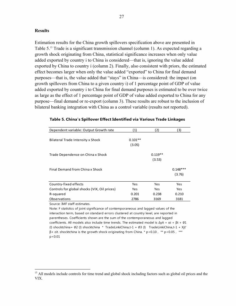
Results Estimation results for the China growth spillovers specification above are presented in Table 5.15 Trade is a significant transmission channel (column 1). As expected regarding a growth shock originating from China, statistical significance increases when only value added exported by country i to China is considered—that is, ignoring the value added exported by China to country i (column 2). Finally, also consistent with priors, the estimated effect becomes larger when only the value added “exported” to China for final demand purposes—that is, the value added that “stays” in China—is considered: the impact (on growth spillovers from China to a given country i) of 1 percentage point of GDP of value added exported by country i to China for final demand purposes is estimated to be over twice as large as the effect of 1 percentage point of GDP of value added exported to China for any purpose—final demand or re-export (column 3). These results are robust to the inclusion of bilateral banking integration with China as a control variable (results not reported).
15 All models include controls for time trend and global shock including factors such as global oil prices and the VIX.
Table 5. China's Spillover Effect Identified via Various Trade Linkages
Dependent variable: Output Growth rate (1) (2) (3)
Bilateral Trade Intensity x Shock 0.101**
(3.05)
Trade Dependence on China x Shock 0.119**
(3.53)
Final Demand from China x Shock 0.148***
(3.76)
Country-fixed effects Yes Yes Yes
Controls for global shocks (VIX, Oil prices) Yes Yes Yes
R-squared 0.201 0.238 0.210
Observations 2786 3169 3181
Source: IMF staff estimates.Note: F statistics of joint significance of contemporaneous and lagged values of the interaction term, based on standard errors clustered at country level, are reported in parentheses. Coefficients shown are the sum of the contemporaneous and lagged coefficients. All models also include time trends. The estimated model is ∆yit = αi + βt + ∅1 (l) shocktchina+ ∅2 (l) shocktchina * TradeLinkiChina,t-1 + ∅3 (l) TradeLinkiChina,t-1 + Xjt' β+ εit. shocktchina is the growth shock originating from China. * p<0.10 , ** p<0.05 , *** p<0.01
28
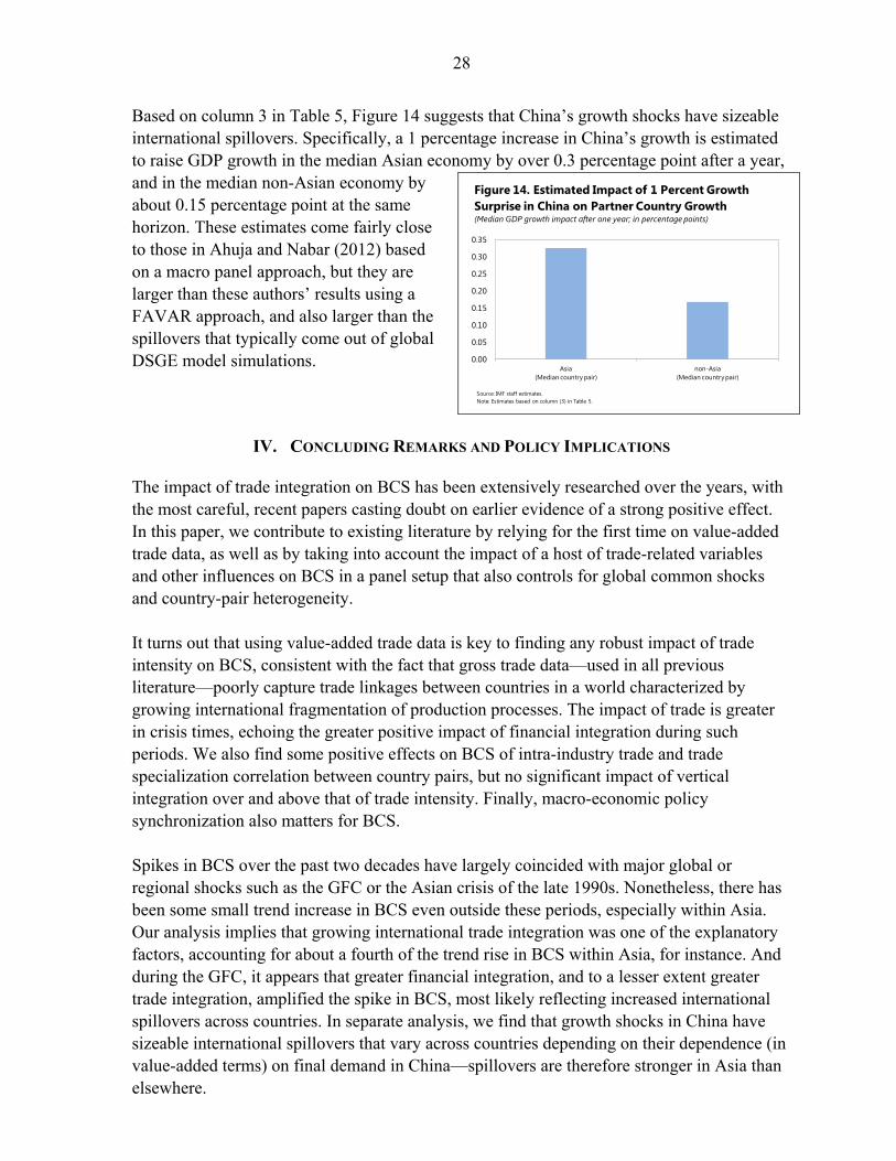
Based on column 3 in Table 5, Figure 14 suggests that China’s growth shocks have sizeable international spillovers. Specifically, a 1 percentage increase in China’s growth is estimated to raise GDP growth in the median Asian economy by over 0.3 percentage point after a year, and in the median non-Asian economy by about 0.15 percentage point at the same horizon. These estimates come fairly close to those in Ahuja and Nabar (2012) based on a macro panel approach, but they are larger than these authors’ results using a FAVAR approach, and also larger than the spillovers that typically come out of global DSGE model simulations.
IV. CONCLUDING REMARKS AND POLICY IMPLICATIONS
The impact of trade integration on BCS has been extensively researched over the years, with the most careful, recent papers casting doubt on earlier evidence of a strong positive effect. In this paper, we contribute to existing literature by relying for the first time on value-added trade data, as well as by taking into account the impact of a host of trade-related variables and other influences on BCS in a panel setup that also controls for global common shocks and country-pair heterogeneity. It turns out that using value-added trade data is key to finding any robust impact of trade intensity on BCS, consistent with the fact that gross trade data—used in all previous literature—poorly capture trade linkages between countries in a world characterized by growing international fragmentation of production processes. The impact of trade is greater in crisis times, echoing the greater positive impact of financial integration during such periods. We also find some positive effects on BCS of intra-industry trade and trade specialization correlation between country pairs, but no significant impact of vertical integration over and above that of trade intensity. Finally, macro-economic policy synchronization also matters for BCS. Spikes in BCS over the past two decades have largely coincided with major global or regional shocks such as the GFC or the Asian crisis of the late 1990s. Nonetheless, there has been some small trend increase in BCS even outside these periods, especially within Asia. Our analysis implies that growing international trade integration was one of the explanatory factors, accounting for about a fourth of the trend rise in BCS within Asia, for instance. And during the GFC, it appears that greater financial integration, and to a lesser extent greater trade integration, amplified the spike in BCS, most likely reflecting increased international spillovers across countries. In separate analysis, we find that growth shocks in China have sizeable international spillovers that vary across countries depending on their dependence (in value-added terms) on final demand in China—spillovers are therefore stronger in Asia than elsewhere.
0.00
0.05
0.10
0.15
0.20
0.25
0.30
0.35
Asia(Median country pair)
non-Asia(Median country pair)
Source: IMF staff estimates.Note: Estimates based on column (3) in Table 5.
Figure 14. Estimated Impact of 1 Percent Growth Surprise in China on Partner Country Growth (Median GDP growth impact after one year; in percentage points)
29
Perhaps the most important implication of these results is that, all else equal, BCS among economies would be expected to continue to rise in the future as world economic integration increases. Trade integration would be a driving force in normal times, and an amplification mechanism in crisis times. Any growth shocks in China would also induce more synchronization as the importance of China as a source of final demand for the rest of the world grows bigger. Finally, future increases in financial integration—especially in emerging economies where it continues to lag behind trade integration, and some catch-up could therefore be expected— could also strengthen spillovers and synchronization in crisis periods, even though they may well reduce co-movement in tranquil times.

30
REFERENCES
Abiad, A., D. Furceri, S. Kalemli-Ozcan, and A. Pescatori, 2013, “Dancing Together? Spillovers, Common Shocks, and the Role of Financial and Trade Linkages,” in World Economic Outlook, (Washington: International Monetary Fund, October), pp. 81–111.
Ahuja, A. and M. Nabar, 2012, “Investment-led Growth in China: Global Spillovers,” IMF
Working Paper 12/267, (Washington: International Monetary Fund). Backus, D., P. Kehoe and F. Kydland, 1992, “International Real Business Cycles,” Journal
of Political Economy, Vol. 100, pp. 745–775. Baxter, M. and M. Kouparitsas, 2005, “Determinants of Business Cycle Co-movement: A
Robust Analysis,” Journal of Monetary Economics, Vol. 52, pp. 113–157. Bordo, M., and T. Helbling, 2010, “International Business Cycle Synchronization in
Historical Perspective,” NBER Working Paper No. 16103, (Massachusetts: National Bureau of Economic Research).
Calderon, C., A. Chong, and E. Stein, 2007, “Trade Intensity and Business Cycle
Synchronization: Are Developing Countries any Different?” Journal of International Economics, Vol. 71, pp. 2–21.
Carter, C. K. and R. Kohn, 1994, “On Gibbs Sampling for State Space Models,” Biometrika,
Vol. 81, pp. 541–553. Di Giovanni, J. and A. Levchenko, 2010, “Putting the Parts together: Trade, Vertical
Linkages and Business Cycle Co-movement,” American Economics Journal: Macroeconomics, Vol. 2, pp. 95–124.
Frankel, J. A., and A. K. Rose, 1997, “Economic Structure and the Decision to Adopt a
Common Currency,” Seminar Paper No 611, The Institute for International Economic Studies (Stockholm: Stockholm University).
–––––––, 1998, “The Endogeneity of the Optimum Currency Area Criteria,” Royal Economic
Society, Vol. 108(499), pp. 1009–1025. Grubel, H. G. and P. J. Lloyd, 1975, Intra-industry Trade: the Theory and Measurement of
International Trade in Differentiated Products, (New York: Wiley). Hirata, H., M. Kose, and C. Otrok, 2013 “Regionalization vs. Globalization,” IMF Working
Paper 13/19, (Washington: International Monetary Fund). Imbs, J., 2004, “Trade, Specialization and Synchronization,” Review of Economics and
Statistics, Vol. 86, pp. 723–734. –––––––, 2006, “The Real Effects of Financial Integration,” Journal of International
Economics, Vol. 68, pp. 296–324.
31
Inklaar, R., R. J-A. Pin, and J. Haan, 2008, “Trade and Business Cycle Synchronization in
OECD countries—A re-examination,” European Economic Review, Vol. 52, pp. 646-666.
International Monetary Fund, 2013, German-Central European Supply Chain—Cluster
Report, IMF Country Report No. 13/263 (Washington, August). Kalemli-Ozcan, Sebnem, B.E. Sorensen, and O. Yosha, 2003, “Risk Sharing and Industrial
Specialization: Regional and International Evidence,” The American Economic Review, Vol. 93, pp. 903–918.
–––––––, E. Papaioannou, and F. Perri, 2013, “Global Banks and Crisis Transmission,”
Journal of International Economics, Vol. 89, pp. 495–510. –––––––, E. Papaioannou, and J. Peydro, 2013, “Financial Regulation, Financial
Globalization, and the Synchronization of Economic Activity,” Journal of Finance, Vol. LXIII, pp. 1179–1228.
Kim, C-J., and C. R. Nelson, 1999, State-Space Models with Regime Switching: Classical
and Gibbs-Sampling Approaches with Applications, (Massachusetts: The MIT Press). Kumakura, M., 2006, “Trade and Business Cycle Co-movement in Asia-Pacific,” Journal of
Asian Economics, Vol. 17, pp. 622–645. McKinnon, R. I., “Optimum Currency Areas,” The American Economic Review, Vol. 53,
pp. 717–725. Mohommad, A., O. Unteroberdoerster, and J. Vichyanond, 2011, “Implications of Asia’s
Regional Supply Chain for Rebalancing Growth,” in Regional Economic Outlook: Asia and Pacific, (Washington: International Monetary Fund, April), pp. 47–60.
Morgan, D., B. Rime, and P. Strahan, 2004, “Bank Integration and State Business Cycles,”
Quarterly Journal of Economics, Vol. 119, pp. 1555–1585. Mundell, R. A., 1961, “A Theory of Optimum Currency Areas,” The American Economic
Review, Vol. 51, pp. 657–665. OECD and WTO, 2012, “Trade in Value-Added: Concepts, Methodologies, and Challenges,”
(OECD-WTO online document). Available via the internet: www.oecd.org/sti/ind/4 9894138.pdf.
Otto, G., G. Voss, and L. Willard, 2001, “Understanding OECD Output Correlations,”
Research Discussion Paper No. 2001–05, (Sydney: Reserve Bank of Australia). Park, Y-C. and K. Shin, 2009, “Economic Integration and Changes in the Business Cycle in
East Asia: Is the Region Decoupling from the Rest of the World,” Asian Economic Papers, Vol. 8:1, pp. 107–140.

32
Shin, K., and Y. Wang, 2003, “Trade Integration and Business Cycle Synchronization in East Asia,” Discussion Paper No. 574, The Institute of Social and Economic Research, (Osaka: Osaka University).
–––––––, 2004, “Trade Integration and Business Cycle Co-movements: The Case of Korea
with other Asian Countries,” Japan and the World Economy, Vol. 16, pp. 213–230. Xing, Y., and N. Detert, 2010, “How the iPhone widens the United States Trade Deficit with
the People’s Republic of China”, ADBI Working Paper Series No. 257, (Manila: Asian Development Bank).

33
APPENDIX I. FURTHER DETAILS ABOUT THE DYNAMIC FACTOR ANALYSIS
Data The source of the expenditure-side real GDP components is IMF WEO data. The database covers the period from 2000Q1 to 2012Q4 and includes 34 countries partitioned into four geographical regions and subgroups: Asia: China, Hong Kong SAR, India, Indonesia, Japan, Korea, Malaysia, Philippines,
Singapore, Taiwan POC, Thailand, Australia, and New Zealand
o China supply- chain: China, Korea, Malaysia, Philippines, Taiwan POC, and Thailand
o ASEAN-5: Indonesia, Malaysia, Philippines, Singapore, and Thailand
o Advanced Asian economies: Hong Kong SAR, Japan, Korea, Singapore, Taiwan POC, Australia, and New Zealand
South America: Brazil, Argentina, Chile, and Venezuela Europe: France, Germany, Greece, Italy, Poland, Portugal, Spain, Sweden, United
Kingdom, Russia, Czech Republic, Hungary, Latvia, and Slovenia North America: Canada, Mexico, and United States
Model and estimation Two types of models are featured in the corresponding section of the main text. Here we present the baseline model without sub-regions, which can be written as follows:
, ~ 0,
, ~ 0,
Where stands for GDP, consumption, and investment growth rates of countries, . stands for factors; and represents residuals. . , . , . are parameters, with the . also called factor loadings. Since both factors and factor loadings have to be estimated, they are only identified by the multiplication ( . . . Their scale and sign are not independently identified. And the scale of a factor also depends on the variance ( ) of the factor equation. Following Hirata and
others (2013), a positive sign is imposed to the factor loading of the first country in a group. The variance ( ) of factor equations is assigned the value estimated during the initialization
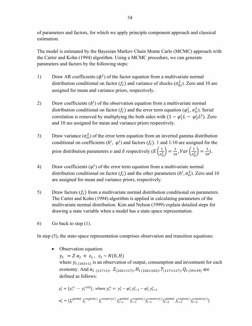
34
of parameters and factors, for which we apply principle component approach and classical estimation. The model is estimated by the Bayesian Markov Chain Monte Carlo (MCMC) approach with the Carter and Kohn (1994) algorithm. Using a MCMC procedure, we can generate parameters and factors by the following steps: 1) Draw AR coefficients ( . ) of the factor equation from a multivariate normal
distribution conditional on factor ( . and variance of shocks ( ). Zero and 10 are
assigned for mean and variance priors, respectively. 2) Draw coefficients ( . ) of the observation equation from a multivariate normal
distribution conditional on factor ( . and the error term equation ( , ). Serial correlation is removed by multiplying the both sides with 1 . Zero and 10 are assigned for mean and variance priors respectively.
3) Draw variance ( ) of the error term equation from an inverted gamma distribution
conditional on coefficients ( . , . ) and factors ( . . 1 and 1/10 are assigned for the
prior distribution parameters and respectively ( , .
4) Draw coefficients ( . ) of the error term equation from a multivariate normal
distribution conditional on factor ( . and the other parameters ( . , ). Zero and 10 are assigned for mean and variance priors, respectively.
5) Draw factors ( . from a multivariate normal distribution conditional on parameters.
The Carter and Kohn (1994) algorithm is applied in calculating parameters of the multivariate normal distribution. Kim and Nelson (1999) explain detailed steps for drawing a state variable when a model has a state-space representation.
6) Go back to step (1). In step (5), the state-space representation comprises observation and transition equations:
Observation equation:
, ~ 0, where is an observation of output, consumption and investment for each
economy. And , , , , are
defined as follows:
∗ ⋯ ∗ , where ∗
. . . . . .

35
. . .⋮ ⋮ ⋮. . .
, where . 0⋯ ⋯ 0⋯ ⋯0
0 0
⋮ ⋱ ⋮0 0
Transition equation
, ~ 0, where , , are defined as follows:
Φ Φ 0
I 0, where Φ . . , 1,2
I
0,
, 0 0⋮ ⋱ ⋮0 0 ,
Additional results Figure A1.1 shows the estimated regional factors in the model with sub-regions. Even though the sub-regional factors are mostly not significantly different from zero except for a few years, China supply-chain and advanced economies show relatively distinguished sub-regional factors, which imply some similarity among the member countries of each group.
As a complementary model, we follow Bordo and Helbling (2010), who combined a VAR approach with the baseline model. Since the model allows for interactions between economic variables as in a usual VAR setup, we can investigate the direct impact of the region’s main economies on their neighbors. To make the model estimable on the relative short sample, we impose some additional simplifying assumptions: the most simple VAR(1) model is applied; only output—not consumption or investment—is considered; no sub-regional factors are

36
Figure A1.1. Regional and Sub-regional Factors (Median and 15 and 85-percent percentiles)
(a) Model with China Supply-chain Sub-region
Regional Factor: Asia China Supply-chain Sub-region
Other Asia
(b) Model with ASEAN-5 Sub-region Regional Factor: Asia ASEAN-5 Other Asia
( c) Model with Asian Advanced/Emerging Sub-region Regional Factor: Asia Advanced Asian Other Asia
Source: IMF staff estimates.
-1.0
-0.5
0.0
0.5
1.0
1.5
20
00
20
01
20
02
20
03
20
04
20
05
20
06
20
07
20
08
20
09
20
10
20
11
20
12
-1.2
-1.0
-0.8
-0.6
-0.4
-0.2
0.0
0.2
0.4
0.6
0.8
20
00
20
01
20
02
20
03
20
04
20
05
20
06
20
07
20
08
20
09
20
10
20
11
20
12
-1.0
-0.8
-0.6
-0.4
-0.2
0.0
0.2
0.4
0.6
0.8
20
00
20
01
20
02
20
03
20
04
20
05
20
06
20
07
20
08
20
09
20
10
20
11
20
12
-1.0
-0.8
-0.6
-0.4
-0.2
0.0
0.2
0.4
0.6
0.8
1.0
1.2
20
00
20
01
20
02
20
03
20
04
20
05
20
06
20
07
20
08
20
09
20
10
20
11
20
12
-1.0
-0.8
-0.6
-0.4
-0.2
0.0
0.2
0.4
0.6
0.8
20
00
20
01
20
02
20
03
20
04
20
05
20
06
20
07
20
08
20
09
20
10
20
11
20
12
-1.0
-0.5
0.0
0.5
1.0
1.5
20
00
20
01
20
02
20
03
20
04
20
05
20
06
20
07
20
08
20
09
20
10
20
11
20
12
-0.8
-0.6
-0.4
-0.2
0.0
0.2
0.4
0.6
0.8
1.0
1.2
20
00
20
01
20
02
20
03
20
04
20
05
20
06
20
07
20
08
20
09
20
10
20
11
20
12
-1.2
-1.0
-0.8
-0.6
-0.4
-0.2
0.0
0.2
0.4
0.6
0.8
1.0
20
00
20
01
20
02
20
03
20
04
20
05
20
06
20
07
20
08
20
09
20
10
20
11
20
12
-1.0
-0.8
-0.6
-0.4
-0.2
0.0
0.2
0.4
0.6
0.8
1.0
20
00
20
01
20
02
20
03
20
04
20
05
20
06
20
07
20
08
20
09
20
10
20
11
20
12

37
included. Since we add the VAR(1) term in the equation, we also drop the dynamics of the error term. Outside of the VAR(1) term, the complementary model thus looks like a simplified version of the baseline model:16
, ~ 0,
, ~ 0,
Even under the simplifying assumptions, the model has still too many explanatory variables. Since the sample includes 34 countries, each observation equation will have 36 explanatory variables (34 lagged variables plus two factors) and will leave only a small number of degrees of freedom. To address this issue, Bordo and Helbling (2010) restrict directly the
by allowing non-zeros only for country i’s own lagged GDP growth rate and one of two variables, namely the “center country” or an important trading partner. In this section, we allow non-zero parameters for the country’s own lagged GDP growth rate, the United States, and the largest economy in each region (China, Brazil, Germany, and Australia, respectively). The estimation method is almost the same as for the baseline model.
Figure A1.2 shows the estimated factors of the complementary model. The global factor is estimated tightly and is similar to that in the baseline model. The Asian regional factor is also consistent with that in the baseline model over the second half of the period, but not clearly distinguished otherwise. In the case of the European factor, there is larger downward trend after the GFC than in the baseline model. Since the factor is the common trend after considering the direct impacts from main economies, the comparison between this and the baseline models suggest that Europe must have benefited from interactions with the United States and German economies after the GFC.
As with the baseline model, we can decompose the unconditional variance with a little additional complication: is a vector which consists of output ( ) of individual countries; is a vector obtained by stacking ; Φ is the matrix comprised of the VAR parameter,
and Σ is a diagonal variance matrix made of :
1 1 ′ 1 1 ′ 1 Σ 1 ′, Φ
16 Even though the baseline model allows for serial correlation in the error term ( , the error terms are restricted to be mutually uncorrelated. So the main difference between the baseline and complementary models is that the latter features the lagged variables on the right-hand side.
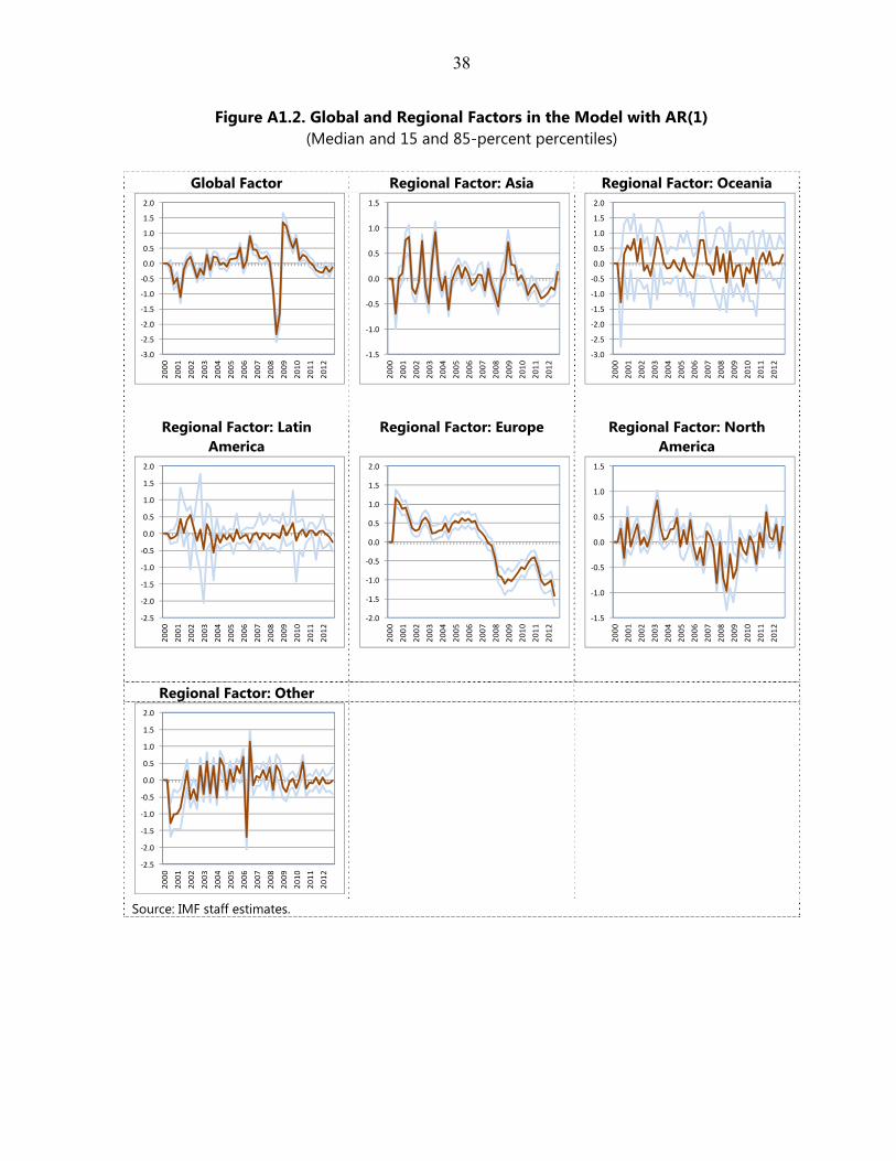
38
Figure A1.2. Global and Regional Factors in the Model with AR(1) (Median and 15 and 85-percent percentiles)
Global Factor Regional Factor: Asia Regional Factor: Oceania
Regional Factor: Latin America
Regional Factor: Europe Regional Factor: North America
Regional Factor: Other
Source: IMF staff estimates.
-3.0
-2.5
-2.0
-1.5
-1.0
-0.5
0.0
0.5
1.0
1.5
2.0
20
00
20
01
20
02
20
03
20
04
20
05
20
06
20
07
20
08
20
09
20
10
20
11
20
12
-1.5
-1.0
-0.5
0.0
0.5
1.0
1.5
20
00
20
01
20
02
20
03
20
04
20
05
20
06
20
07
20
08
20
09
20
10
20
11
20
12
-3.0
-2.5
-2.0
-1.5
-1.0
-0.5
0.0
0.5
1.0
1.5
2.0
20
00
20
01
20
02
20
03
20
04
20
05
20
06
20
07
20
08
20
09
20
10
20
11
20
12
-2.5
-2.0
-1.5
-1.0
-0.5
0.0
0.5
1.0
1.5
2.0
20
00
20
01
20
02
20
03
20
04
20
05
20
06
20
07
20
08
20
09
20
10
20
11
20
12
-2.0
-1.5
-1.0
-0.5
0.0
0.5
1.0
1.5
2.0
20
00
20
01
20
02
20
03
20
04
20
05
20
06
20
07
20
08
20
09
20
10
20
11
20
12
-1.5
-1.0
-0.5
0.0
0.5
1.0
1.5
20
00
20
01
20
02
20
03
20
04
20
05
20
06
20
07
20
08
20
09
20
10
20
11
20
12
-2.5
-2.0
-1.5
-1.0
-0.5
0.0
0.5
1.0
1.5
2.0
20
00
20
01
20
02
20
03
20
04
20
05
20
06
20
07
20
08
20
09
20
10
20
11
20
12

39
Each variance component is further divided into impacts through the country’s own lags and through the major countries’ lags. The impact through the country’s own lags is calculated by setting non-diagonal components of Φ to zero. Table A1.1 shows the variance decomposition results. The transmission of the global factor has impacts on economies through both their own lags and those of the major countries. Unlike in the baseline model, the influence of the global factor on Asian economies is not smaller than on its impact on European economies. By contrast, similar to the baseline model and consistent with Figure A1.2, the explanatory power of the Asia regional factor is relatively small, consistent with a continued key role played by global factors in driving the regional cycle. However, this does not necessarily mean that large Asian economies like China do not have a major influence on their neighbors, as their impact might partly be reflected in the global factors—and might also have become sizeable only in very recent years, something which cannot be adequately captured here as our estimation and variance decomposition are performed over the full period 2000–12.
Table A1.1. Variance Decomposition in the Model with AR(1)
Own Trasmission Sum Own Trasmission Sum
World 0.17 0.20 0.37 0.16 0.07 0.23 0.60
Asia 0.22 0.20 0.41 0.09 0.07 0.17 0.58
Oceania 0.03 0.11 0.15 0.27 0.10 0.37 0.52
Latin America 0.15 0.11 0.25 0.20 0.04 0.24 0.49
Europe 0.14 0.24 0.38 0.17 0.07 0.24 0.63
North America 0.22 0.20 0.42 0.19 0.09 0.28 0.70
Others 0.21 0.19 0.40 0.24 0.07 0.31 0.71
Global RegionalSum

40
APPENDIX II. FURTHER DETAILS ON THE DATA
Trade integration The main trade variables in our dataset employ trade in value-added indicators from the second release of the OECD-WTO TiVA database (released on May 2013). Unlike gross trade data, value-added trade data do not count products multiple times when they cross borders repeatedly for processing purposes (OECD-WTO, 2012). The bilateral trade intensity and vertical integration variables used throughout Section [III] are constructed using several OECD-WTO TiVA indicators listed below, all of which cover both goods and services:
Domestic Value Added Embodied in Gross Exports (DVA): At the country level, it can be simply defined as the sum of two contributions: i) the direct contribution from industries that produce exported goods and services; ii) the indirect contribution from domestic supplier industries made through domestic upstream transactions. At the industry level, which is not used in this paper, a third component—that cancels out upon aggregation at the country level—is the domestic value added that was exported in goods and services used to produce the intermediate imports of goods and services used by the industry in question (i.e., re-imports).
Foreign Value Added Embodied in Gross Exports by partner country (FVA): foreign value added embodied in exports broken down by country of origin (i.e., the import content).
Gross Exports [as estimated in OECD-WTO TiVA database] (GR): the sum of total domestic value added and total foreign value added embodied in exports.
Domestic Value Added Embodied in Foreign Final Demand (DVA_FD): the domestic (i.e., country i) value added embodied in foreign (i.e., country j) final domestic demand. It is the sum of two types of value added: i) direct exports of final goods and services from country i to j; ii) exports of intermediate goods from country i to other countries that will eventually be re-exported to country j for final consumption.
While the OECD-WTO TiVA database provides invaluable data on exports in value-added terms, the database only covers years 1995, 2000, 2005, 2008, and 2009. In order to construct an annual database covering the years 1995–2012, we construct the variables mentioned above following as closely as possible the OECD-WTO methodology and concepts but using trade data from an alternative, annual database, namely the United Nation’s COMTRADE. The series we obtain can be viewed as proxies for the OECD-WTO data. We then use these

41
series’ profile to interpolate the OECD-WTO data between available years, and also to extrapolate beyond 2009. We obtain full annual series over 1995–2012. 17
Concretely, we use UN COMTRADE gross trade data classified according to the Harmonized System (HS) and converted to International Standard Industrial Classification (ISIC), in line with the SNA1993 manual and the industries used in OECD-WTO TiVA database. Using this data along with data classified in accordance with SITC, we construct total exports, final goods exports, intermediate exports, and intermediate imports. To do so, we incorporate classification correspondence tables developed by the United Nations Statistics Department (i.e., HS, ISIC, CPC, SITC, and BEC correspondence tables are used).
Based on these data, the DVA series for each industry is then estimated as the sum of three subcomponents. The domestic direct and domestic indirect components in industries are interpolated using the growth of total exports less intermediate imports, while the re-imported domestic component is derived using intermediate exports growth. The FVA series is estimated by interpolating the foreign value added with intermediate imports growth. The (OECD-WTO-consistent) gross exports series is estimated by interpolating value-added data with total exports growth. The time series for DVA in Foreign Final Demand is estimated by interpolating its value-added series with the final goods exports growth.
Another trade variable in our empirical analysis, namely the Grubel and Lloyd index (GL index), relies on bilateral gross trade data from the UN COMTRADE database using SITC, Rev.3 at a 3-digit level. The index is constructed by adjusting for the inconsistency issues of mirror trade data due to asymmetry in reporting exports and imports in trade statistics (i.e., imports of country i from j usually differ from the exports reported from j to i). Our adjustment is rather simple, where the index is constructed using both country i and country j’s trade data and the average of the two values for each year is taken. As a robustness check, we also constructed GL indices using the minimum and the maximum of the two, as well as simply using the GL index of the high-income country within the pair as done by Calderon and others (2007); the results remain robust in all cases.
As a robustness check, we also constructed GL indices at different levels of disaggregation up to the 5-digit level and for different coverage of goods; results using these alternative indices remained broadly unchanged as well. The rationale for ultimately using the 3-digit GL index in our empirical analysis is two-fold: i) the 3-digit GL index for all goods is widely used in trade literature, ii) it is the level of disaggregation used for another explanatory trade variable, namely the Trade Specialization Correlation Index, which we take directly from the United Nations Conference on Trade and Development’s UNCTADstat database.
17 Robustness of the regressions using these interpolated series is validated using four-period panel regressions (see Appendix III).
42
Financial integration
Banking integration data are based on bilateral locational banking statistics by residency from BIS unpublished databases. Using locational data by residency is conceptually consistent with the residency principle of national accounts and the balance of payments. We have total bilateral external positions (both assets and liabilities separately) over 1990– 2012 for BIS-reporting countries vis-à-vis individual partner countries. Based on these data, the banking integration variable is defined as below:
Banking Integration: defined as in Abiad and others (2013) as the ratio of the stock of bilateral assets and liabilities between countries i and j in year t to the sum of these two countries’ external assets and liabilities vis-à-vis the entire world in the previous year t-1:
where is bilateral banking integration between countries i and j in year t,
is the stock of assets and liabilities of country i’s banks vis-à-vis country j, and is the total stock of asset and liabilities of country i vis-à-vis the world in
year t-1.
Portfolio integration data are based on the bilateral portfolio investment positions (both equity and debt securities) provided by reporting economies to the IMF’s Coordinated Portfolio Investment Survey (CPIS), in line with the residency principle of the balance of payments. We use all available bilateral positions in the CPIS database starting as early as 2001. The portfolio integration variable is then defined as follows:
Portfolio Integration: between countries i and j, computed as:
where denotes the investment holdings (equity and debt securities) of country i in country j.
FDI integration data are based on the bilateral direct investment positions provided by the reporting economies to the IMF’s Coordinated Direct Investment Survey (CDIS), in line with the residency principle of balance of payments. The CDIS initiative, launched in late 2010, only covers bilateral direct investment positions starting from 2009. Therefore, for the years 2000-2008, we construct the bilateral direct investment position series using data from the now discontinued bilateral direct investment statistics from the UNCTAD and the OECD. The FDI integration variable is then defined as follows:
FDI Integration: between countries i and j, defined as:
43
where is the FDI stock held by country i in country j.
Macroeconomic policy synchronization
Fiscal policy synchronization, , for countries i and j in year t is defined as the quasi-correlation (as defined for the dependent variable, quasi-correlation of output) of the structural fiscal balances (in percent of potential GDP) of the two countries purged from the impact of the cycle—to focus more closely on fiscal policy shocks and address possible reverse causality:
∗ ∗ ∗
∗
where fit is the structural balance of country i in year t purged from the impact of the cycle by regressing the structural balance on the output gap (both using IMF WEO
data), ∗ and are, respectively, the average and standard deviation of the structural balance of country i over the sample period.
Monetary policy synchronization between two countries is defined as the negative of the absolute difference in the short-term real interest rate of the two countries, -|rit-rjt |, where rit and rjt are respectively the short-term real interest rates of countries i and j in year t purged from the impact of the cycle. This should mitigate the endogeneity of the monetary policy variable to cyclical fluctuations—an alternative, costlier approach would have been to estimate for example, monetary policy rules for each country, and to compute the synchronization variable using the residual series.
The exchange rate rigidity variable is measured as the negative of the volatility of monthly nominal bilateral exchange rates. Specifically, for a country pair i-j and year t, it is defined as the standard deviation of the monthly changes in the nominal bilateral exchange rate between i and j during year t.
Instrumental variables
As mentioned in Section III.B above, following the traditional gravity approach, we instrument trade intensity with a geographical distance index, the degree of trade cooperation between countries, a time-varying dummy for the membership to the WTO, the average import tariff of the two countries, the average intermediate goods import tariff of the two countries, and the product of their real GDPs:
Geographical distance index: following Wei (1996) and Deardoff (1998), the geographical distance index of country i is defined as the sum of the physical distances of country i from all its trade partners (except country j), weighted by the
44
share of trade partners in world GDP. Similarly, geographical distance index of country j is defined as the sum of the physical distances of country j from all its trade partners (except country i), weighted by the share of trade partners in world GDP. Bilateral distance is the distance between the most important cities (in terms of population) of the two countries, which is obtained from CEPII’s GeoDist database.
Degree of trade cooperation: the index is constructed using information on regional trade agreements (RTAs) coming from the WTO’s RTA database. Based on the type of RTAs, we construct the degree of trade cooperation variable on a scale of 0 to 5, where 5 indicate the highest degree of cooperation. Specifically, a score of 5 indicates that the two countries belong to a Currency Union and Economically Integrated Area starting year t, 4 indicates that the two countries are integrated in the form of a Currency Union only, 3 is for countries that are in a Free Trade Area and Economically Integrated Area, 2 indicates that the countries are in a Free Trade Area only, 1 indicates a Partial Scope Agreement between the countries, and 0 represents No trade agreement.
Import tariffs (both total and intermediate goods): data starting 1995 are obtained from the WTO Integrated Database (IDB) and the TRANS database. We obtain tariff data for all countries in our sample based on HS classifications, further refined in the case of tariffs applied only to intermediate goods.

45
APPENDIX III. ROBUSTNESS FOR ECONOMETRICS—USING FOUR PERIODS
Robustness Check In order to check the robustness of our findings on annual data and to facilitate comparisons with previous studies, we also construct another output co-movement index using Pearson correlations of quarterly growth rates. Four periods are considered here: 1990–96, 1997-2000, 2001-07 and 2008-12. Over each of these, we compute:
CORR corr g , g
where CORR is the Pearson correlation coefficient for quarterly growth rates of countries i
and j in period τ, and g is the growth rate of country i in quarter t of period τ. The model used for determining the effect of trade integration on business cycle is the same as in equation (1) with ‘t’ replaced with τ. The right-hand side variables are values averaged over period τ for all variables, except for “trade intensity.” Since the raw OECD-WTO TiVA data are available only for five years, we use only those here so as to check whether our findings are also robust to not interpolating the actual data. So, for the periods 1990–96, 1997-2000, 2001–07 and 2008–12 we use OECD-WTO trade intensity values for the years 1995, 2000, 2005 and (an average of) 2008–09, respectively. Table A3.1 shows that these four-period panel regressions yield results that are broadly in line with those based on annual data.
OLS IV OLS IV
(1) (2) (3) (4)
Trade Intensity 0.0585** 0.271*** 0.0500* 0.254***(0.0270) (0.0726) (0.0270) (0.0731)
Banking Integration -0.00514 -0.00929 -0.00309 -0.00759(0.0124) (0.00955) (0.0124) (0.00960)
Intra-industry Trade 0.00522*** 0.00362**(0.00183) (0.00154)
Trade Specialization Correlation 0.157 0.142(0.168) (0.131)
Global Financial Crisis Dummy 0.389*** 0.386*** 0.377*** 0.377***(0.0133) (0.0105) (0.0143) (0.0112)
Country-fixed effects Yes Yes Yes YesTime-fixed effects Yes Yes Yes YesFirst-stage F-statistic 26.81 29.9R-squared 0.63 0.60 0.64 0.60Observations 2034 1746 2034 1746Source: IMF staff estimates.
* p<0.10 , ** p<0.05 , *** p<0.01
Table A3.1. Business Cycle Synchronization and Trade Integration - Regressions over Four-time Periods
Dependent Variable: Correlation of quarterly growth rates of output
Standard errors, clustered at country-pair level, are given in parentheses. Global financial crisis represents period 2008-12.


