51

-i-
Acknowledgements
I would like to thank the Institute of Developing Economies (IDE)-Japan External Trade
Organization (JETRO) for the opportunity to carry out this research as a Visiting Research
Fellow. Carrying out this research here gave me insight into the IDE-JETRO’s development
related contributory activities towards developing countries.
I would like to extend my thanks to my counterpart Etsuyo Michida, research fellows
Yasushi Hazama, Michikazu Kojima, Tomohiro Machikita, Kaoru Murakami, Sanae Suzuki
for their helpful approaches and international exchange department for its guidance. Most of
all, I would like to thank my family, Aya and Kaan, for their support and the inspiration.
Cemal Atici

-ii-
Table of Contents
Contents Page
Acknowledgements……………………………………………………………………….…..
Table of Contents…………………………………………………………………………….
List of Tables…………………………………………………………………………………
List of Figures…………………………………………………………………………………
Abstract …………………………………………………………………………………..….
Introduction………………………………………………………………………………….
1. Review of Literature…………………………………………………………………….
2. Overview of the ASEAN ……………………………………………………………….
2.1 History…………………………………………………………………………….
2.2 Main Economic Indicators…………………………………………………………
2.3 Environment…………………………………………………………………….…
2.3.1 The Environmental Performances…………………………………………
2.3.2 The Environmental Situation in the Region………………………………
2.3.2.1 Fresh Water and Marine Ecosystems………………….…………
2.3.2.2 Terrestrial Ecosystems……………………………………………
2.3.2.3 Atmosphere………………………………………………………
2.3.2.4 Sustainable Production and Consumption………………………
3. Method…………………………………………………………………………………..
4. Results…………………………………………………………………………………...
4.1. Carbon Emissions…………………………………………………………………
4.1.1 Japan’s CO2 Emissions……………………………………………………
4.1.2 ASEAN CO2 Emissions……………………………………………………
4.2 Agricultural Emissions…………………………………………………………….
4.3 Dynamic Estimation………………………………………………………………
Conclusions …………………………………………………………………….…………...
References………………………………………………………………………………..…..
ⅰ
ⅱ
ⅲ
ⅴ
ⅵ
1
2
7
7
8
12
12
13
13
14
15
15
17
21
21
24
25
30
34
37
39

-iii-
List of Tables
page
Table 1: Main Economic Indicators of Japan and ASEAN, 2008............................................. 9
Table 2: Total and Agricultural Trade Values of Japan and ASEAN Members, 2007,
1000$......................................................................................................................... 9
Table 3: Share of Export to GDP in Japan and ASEAN Members, 2008……………….........10
Table 4: Japan-ASEAN Trade Flow, 2008, $............................................................................11
Table 5: Japan’s Main Import Items from ASEAN, 2008, US$..............................................11
Table 6: Main Agricultural Items Exported and Imported in Japan and ASEAN, 2007…......12
Table 7: Environmental Performance Indices of Japan and ASEAN Members, 2010….........13
Table 8: The Overview of Selected Environmental Indicators in Japan and ASEAN,
2008……………………...…………………………………..……………………....16
Table 9: Summary Statistics……….…………………………………………........…..…........24
Table 10: Correlation Matrix of ASEAN CO2 Emission (n=370)……….………..………….24
Table 11: Japan’s Carbon Emission Per Capita Regression Results
(Dependent variable ln- CO2 per capita)…….………………………….…………..25
Table 12: ASEAN CO2 Emissions Panel Regression Results
(Dependent variable ln- CO2 per capita)........……..…….………………………….27
Table 13: ASEAN-D2 CO2 Emissions Panel Regression Results
(Dependent variable per ln- CO2 capita)………………………………………..….28
Table 14: ASEAN-D4 CO2 Emissions Panel Regression Results
(Dependent variable ln- CO2 per capita)………….………………………..……….29

-iv-
Table 15: ASEAN-LD4 CO2 Emissions Panel Regression Results
(Dependent variable ln- CO2 per capita).……………………….…………………..30
Table 16: ASEAN Agricultural Nitrate Emissions Panel Regression Results
(Dependent variable ln-nitrous-oxide per capita)……….………………………….32
Table 17: ASEAN Agricultural Nitrate Emissions Panel Regression Results,
Excluding Singapore (Dependent variable ln-nitrous-oxide per capita)…….…..…33
Table 18: ASEAN Agricultural Methane Emissions Panel Regression Results
(Dependent variable ln-methane per capita)…….…………….…………..……….33
Table 19: ASEAN Agricultural Methane Emissions Panel Regression Results,
Excluding Singapore (Dependent variable ln-methane per capita).…….….………34
Table 20: A-B GMM Dynamic Panel Estimation of Emissions for ASEAN.…..……………36

-v-
List of Figures
Page
Figure 1: The EPI Indicators, % ………………….………………………….………………..12
Figure 2: Environmental Kuznets Curve………………………….……………………….…..17
Figure 3: The EKC with N Shape……………………………………………………………..18
Figure 4: CO2 Emissions in ASEAN, 1970-2006, kt………………………………….………21
Figure 5: CO2 Emissions Per Capita in ASEAN, 1970-2006, kg……………………….…….22
Figure 6: Japan’s CO2 Emissions, kt, 1960-2006……………………………………….…….22
Figure 7: Japan’s CO2 Emissions Per Capita, 1960-2006…………………….……….………23
Figure 8: The Export Share of Polluting Industries in Total Exports in ASEAN,
1967-2006………………………………………………………….…….………….23
Figure 9: Agricultural Nitrous Oxide Emissions, CO2 Equivalent, kt……….………….…….31
Figure 10: Agricultural Methane Emissions, CO2 Equivalent, kt…………….……….………31

-vi-
Abstract
This study examines the trade-environment interaction in the ASEAN region employing
extended Environmental Kuznets Curve (EKC) and utilizing panel data. The examination of
environmental situation in the region indicates that the region faces some environmental
problems such as population growth, increasing industrial activities, and climate change.
However, the introduction of new regulations, stricter standards, and promoting renewable
energy measures being implemented in the region can help sustainable development. The
results indicate that carbon emissions display inverted S shape such that the emission levels
per capita decrease with higher GDP in all groups. However, the turning point income levels
vary depending on the country group. In general the share of exports to the GDP is main
contributor for carbon emission reflecting the negative externality of export based growth. On
the other hand, the trade with Japan has no significant impact on the emission levels implying
that Japan’s import does not stimulate the pollution level in the region. Furthermore, the
results demonstrate that the FDI has no deteriorating impact on emission levels. In terms of the
agricultural emissions, it is observed that the emission levels confirm the conventional EKC
(inverted U shape). In addition, high tariff levels increase the pollution of nitrous oxide
meaning that protection leads to higher domestic production and consequently high level of
input use that intensifies the pollution. Agricultural subsidies and laxity of regulations also
have polluting impacts in the region. The dynamic regression indicates that the pollution of the
carbon dioxide and nitrous oxide in previous years will cause pollution in current year because
of the cost of eliminating pollution. Given the fact that production requires energy use, the
region needs environmentally friendly technologies for energy production. This can be
achieved by more research and development expenditures as well as regional collaboration.
Since agricultural subsidies and laxity of regulations increase the pollution level in the region,
input related subsidies should be reconsidered and agricultural related regulations should be
implemented. In this process regional collaboration, technical assistance, and guidance are
crucial for the sustainable development of the region.
-1-
Introduction
Current path of globalization has raised the trade flow among the countries
including the developing ones. However, such an increase can cause environmental
problems because of the higher production and trade activities. Trade policies such as tariffs
or setting standards on export and import also impact production, consumption, and trade,
and consequently change the levels of nitrogen and carbon dioxide emissions. These
pollutants lead to the health and environmental problems. Since many developing countries
have comparative advantage in pollution intensive goods, production of goods may shift to
the developing world as a consequence of trade liberalization. However, as trade
liberalization leads to higher income that wealth can raise the environmental awareness as
well. Agricultural trade activities impact environmental quality since pollutants caused by
trade activities directly affect the natural resources such as land and water. Increasing
agricultural trade flow will have various impacts on the environmental quality in ASEAN
members and its trade partners. Japan, on the other, is an important trade partner for the
ASEAN members (Comtrade, 2010). Although some recent studies (Grossman and Krueger,
1991; Panayotu, 1995; Torras and Boyce, 1998; Anderson, 2001; Cole 2003-2004; Taylor,
2004; Paudel et al. 2005) examined economic growth, trade and environmental interaction,
environmental decay caused by agricultural trade flow and globalization which directly
impacts natural resources such as water and land, is the area which needs further and
detailed examination. The originality of this study stems from its aim to explore the impact
of total and agricultural trade flow on environmental decay in Japan and ASEAN countries
comparatively. It is expected that the result of this study will contribute designing
sustainable environmental trade policies in the region. The main objective of the study is to
determine the trade-off between the trade liberalization and environmental pollution in Japan
and selected ASEAN countries comparatively. The specific objectives are: to determine the
flow of aggregate and agricultural trade related pollutants such as CO2, nitrogen, and
methane pollutants in Japan and ASEAN countries, considering this region’s trade flow
with Japan, to examine the trade-environment interaction employing an extended
Environmental Kuznets curve, to explore the optimum level of trade per capita and income
that determines threshold level of environmental pollution and recommend optimal trade
policies to improve environmental quality.

-2-
1. Review of Literature
Usually, the EKC was estimated to examine and test the income-environmental
relationships. Grossman and Krueger’s (1991) study of air quality and income interaction
was an early example of that kind of studies. Also Shafik and Bandyopadhyay (1992) and
Panayotu (1995) further examined environment growth relationships. Many other studies
examined the Kuznets curve for different pollutants. For instance, Torras and Boyce (1998),
Anderson (2001), Paudel et al. (2005) examined water pollution employing the Kuznets
curve. Copeland and Taylor (2004) reviewed the trade and environment interaction and
some other studies such as Cole (2003-2004) and Atici (2009) carried out empirical studies
on trade related pollution. Recent studies examined the EKC in a panel data context as more
data available on the subject.
In terms of panel version of Kuznets curve there have been some studies. Selden
and Song (1994) investigate the EKC using a cross-national panel of data on emissions of
four important air pollutants: suspended particulate matter, sulfur dioxide, oxides of nitrogen,
and carbon monoxide. They find that per capita emissions of all four pollutants exhibit
inverted-U relationships with per capita GDP. While this suggests that emissions will
decrease in the very long run, their forecast indicates a rapid growth in global emissions over
the next several decades. Matyas (1998) tested Kuznets’ U-curve hypothesis on two
unbalanced panel data sets of 47 and 62 countries, for the period 1970-93, using two-way
fixed and random effects models. It is shown that there is no hard empirical evidence to
support the usual econometric model formulations and the U-curve hypothesis. List (1999)
uses a new panel data set on state-level sulfur dioxide and nitrogen oxide emissions from
1929-1994. The findings suggest that previous studies, which restrict cross-sections to
undergo identical experiences over time, may be presenting statistically biased results. Barro
(2000) indicates that the EKC hypothesis does not explain the bulk of variations in
inequality across countries or over time. Thornton’s (2001) study using panel data set of
Gini coefficients, income quintiles and real GDP per capita in 96 countries over the postwar
period, suggest that the relation between income inequality and development corresponds to
an inverted-U, as hypothesized by Kuznets. Perman and Stern (2003) use cointegration
analysis to test the EKC hypothesis using a panel dataset of sulfur emissions and GDP data
for 74 countries over a span of 31 years. They find that the data is stochastically trending in
the time-series dimension. Given this, and interpreting the EKC as a long run equilibrium
relationship, support for the hypothesis requires that an appropriate model cointegrates and
that sulfur emissions are a concave function of income. Their study suggests that even they
find cointegration; many of the relationships for individual countries are not concave. The
results show that the EKC does not support the case of sulfur emissions.

-3-
Halkos (2003) uses a large database of panel data consisting of 73 OECD and non-
OECD countries for the period of 1960-1990 and apply for the first time random coefficients
and Arellano-Bond Generalized Method of Moments (A-B GMM) econometric methods.
The findings indicate that the EKC hypothesis is not rejected in the case of the A-B GMM.
On the other hand there is no support for an EKC in the case of using a random coefficients
model. Their turning points range from $2805-$6230 per capita. Romero-Avila (2008)
investigates the time series properties of per capita CO2 emissions and per capita GDP levels
for a sample of 86 countries over the period 1960-2000. For that purpose, they employ a
panel stationary test which incorporates multiple shifts in level and slope, thereby
controlling for cross-sectional dependence through bootstrap methods. Their analysis renders
clear evidence that per capita GDP levels are nonstationary for the world as a whole while
per capita CO2 is found to be regime-wise trend stationary. The analysis of country-groups
shows that for Africa and Asia, per capita CO2 is best described as no stationary, while per
capita GDP appears stationary around a broken trend. In addition, they find evidence of
regime-wise trend stationarity in both variables for the country-groups consisting of America,
Europe and Oceania.
Mazzanti’s (2008) study provides new empirical evidence on Environmental
Kuznets Curves (EKC) for greenhouse gases and other air pollutant emissions in Italy. A
panel dataset based on the Italian NAMEA (National Accounts Matrix including
Environmental Accounts) for 1990-2001 is analyzed. The highly disaggregated dataset (29
production branches, 12 years and nine air emissions) provides a large heterogeneity and can
help to overcome the shortcomings of the usual approach to EKC based on cross-country
data. Both value added and capital stocks per employee are used as alternative drivers for
analyzing sectoral NAMEA emissions. Trade openness at the same sectoral level is also
introduced among the covariates. They find mixed evidence supporting the EKC hypothesis.
The analysis of NAMEA-based data shows that some of the pollutants such as two
greenhouse gases (CO2 and CH4) produce inverted U-shaped curves with coherent within-
range turning points. Other pollutants (SOX, NOX, PM10) show a monotonic or even N-
shaped relationship. Macro sectoral disaggregated analysis highlights that the aggregated
outcome should hide some heterogeneity across different groups of production branches
(industry, manufacturing, and services). Services tend to present an inverted N-shape in most
cases. Manufacturing industry shows a mix of inverted U and N-shapes, depending on the
emission considered.
Halkos and Tzeremes (2009) examine the long-run effects of large-scale structural
change with and without international capital accumulation, mobility and ownership. They
demonstrate the relative merits and limitations of different treatments of international capital
accumulation, mobility and ownership. Their findings support the work of Baldwin and
others who have demonstrated that ignoring capital accumulation, mobility and ownership
underestimates net output and welfare effects of large-scale structural change.

-4-
Lee at al. (2009) apply the dynamic panel generalized method of moments
technique to reexamine the environmental Kuznets curve (EKC) hypothesis for carbon
dioxide emissions and asks two critical questions: "Does the global data set fit the EKC
hypothesis ?" and "Do different income levels or regions influence the results of the EKC ?"
They find evidence of the EKC hypothesis for CO2 emissions in a global data set, middle-
income, and American and European countries, but not in other income levels and regions.
Thus, the hypothesis that one size fits all cannot be supported for the EKC. Managi and
Kaneko (2009) analyze how the performance of environmental management has changed
over time using province level data for 1992-2003 for China. Mixed results for
environmental performance are shown using nonparametric estimation technique. They find
that environmental performance index, abatement effort, and increasing returns to pollution
abatement play important roles in determining the pollution level over the period of the study.
In another related study Lee et al (2010) examines the environmental Kuznets curve (EKC)
hypothesis for water pollution by using a recent generalized method of moments dynamic
technique, for a sample of 97 countries during the period 1980-2001. The empirical results
show evidence of the inverted U-shaped EKC relationships existence in America and Europe,
but not in Africa and Asia and Oceania. Thus, the regional difference of EKC for water
pollution is supported. Furthermore, the estimated turning points are, approximately,
US$13.956 and US$38.221 for America and Europe, respectively.
In terms of trade and environment there have been some studies. Muradian and
Martinez (2001) argue that neither environmental economics nor ecological economics take
into account the structural conditions determining the international trade system. Based on
some new empirical evidence on material flows, they stress the notion of environmental
cost-shifting. Cole (2003) assesses the strength of the Environmental Kuznets Curve (EKC)
which posits an inverted-U relationship between per capital income and pollution.
Specifically, answers are sought to the following related questions: (1) How robust is the
EKC relationship? (2) To what extent can the EKC relationship be explained by changing
trade patterns as opposed to growth-induced pollution abatement? The results indicate that
the inverted-U relationship between per capita income and emissions is reasonably robust
and little evidence is found to suggest that trade patterns are a significant determinant of the
inverted-U shape. Dinda (2004) reviews some theoretical developments and empirical
studies dealing with EKC phenomenon. Evidence of the existence of the EKC has been
questioned from several points, and only some air quality indicators, especially local
pollutants, show the evidence of an EKC. Dobson and Rablogan (2009) test the Kuznets
hypothesis in the context of trade liberalization using data for Latin America. The evidence
is consistent with the Kuznets hypothesis. The curvilinear relationship between openness and
inequality suggests that Latin American countries should continue with trade liberalization
measures but also introduce redistribution policies to ease the adverse consequences of
liberalization. Atici (2009) examines the impact of various factors such as gross domestic

-5-
product per capita, energy use per capita, and trade openness on carbon dioxide emission per
capita in the Central and Eastern European Countries. The extended Environmental Kuznets
Curve (EKC) was employed utilizing the available panel data from 1980 to 2002 for
Bulgaria, Hungary, Romania, and Turkey. The results confirm the existence of an EKC for
the region such that CO2 emission per capita decreases over time as the per capita GDP
increases. Energy use per capita is a significant factor that causes pollution in the region
indicating that the region produces environmentally unclean energy. The trade openness
variable implies that globalization did not facilitate the emission level in the region. The
results imply that the region needs environmentally cleaner technologies in energy
production to achieve sustainable development.
In terms of Japan and ASEAN region there have been some panel studies as well.
For instance Coondoo and Dinda (2002) examine a study of income-CO2 emission causality
based on a Granger causality test to cross-country panel data on per capita income and the
corresponding per capita CO2 emission data. Their results indicate three different types of
causality relationship holding for different country groups. For the developed country groups
of North America and Western Europe the causality is found to run from emission to income.
For the country groups of Central and South America, Oceania and Japan causality from
income to emission is obtained. In terms of the country groups of Asia and Africa the
causality is found to be bi-directional. The regression equations estimated as part of the
Granger causality test further suggest that for the country groups of North America and
Western Europe the growth rate of emission has become stationary around a zero mean, and
a shock in the growth rate of emission tends to generate a corresponding shock in the growth
rate of income. In contrast, for the country groups of Central and South America, Oceania
and Japan a shock in the income growth rate is likely to result in a corresponding shock in
the growth rate of emission. Tamazian (2009) using standard reduced-form modeling
approach and controlling for country-specific unobserved heterogeneity, investigate the
linkage between not only economic development and environmental quality but also the
financial development. Panel data over period 1992-2004 is used. They find that both
economic and financial developments are determinants of the environmental quality in BRIC
economies. Their results show that higher degree of economic and financial development
decreases the environmental degradation. The financial liberalization and openness are
essential factors for the CO2 reduction. The adoption of policies directed to financial
openness and liberalization to attract higher levels of R&D-related foreign direct investment
might reduce the environmental degradation in countries under consideration. In addition,
the robustness check trough the inclusion of US and Japan does not alter main findings.
Although there is a large body of literature on emission level and income
relationship, the examination at sectoral and regional level is needed. Specifically, pollutants
caused by increasing total and agricultural trade flow needs to be evaluated in an extended
view. This study therefore aims to explore that relationship employing an extended EKC

-6-
utilizing panel data for Japan and selected ASEAN countries. By carrying out that research
we can obtain some results related to the trade and environment interaction such as the
impact of income, trade openness, and environmental standards on the level of
environmental pollutants. Then, it is possible to calculate threshold level of income and trade
activity that impacts the level of pollutants. The finding of this study is expected to help
designing sustainable policies in the region.

-7-
2. Overview of the ASEAN
2.1. History
The main rationale behind the emergence of economic regionalism in the region can
be explained by the deepening of regional economic interdependence in East Asia. The
intraregional trade as a share of East Asia’s total trade has risen from 35 % in 1980 to 55 %
in 2004 and it is higher than North American Free Trade Area (46 %) (Kawai, 2006). The
Association of Southeast Asian Nations (ASEAN) was established on 8 August 1967 in
Bangkok, Thailand, with the signing of the ASEAN Declaration by the founding members,
namely Indonesia, Malaysia, Philippines, Singapore and Thailand. Brunei Darussalam
joined on 8 January 1984, Vietnam on 28 July 1995, Lao PDR and Myanmar on 23 July
1997, and Cambodia on 30 April 1999. Thus number of members has reached to ten.
According to the ASEAN Declaration the aims and purposes of ASEAN is to accelerate
the economic growth, social progress and cultural development in the region, promote
regional peace and stability through abiding respect for justice and law in the relationship
among countries of the region and adherence to the principles of the United Nations Charter,
the expansion of their trade, including the study of the problems of international commodity
trade, the improvement of their transportation and communications facilities and the raising
of the living standards of their peoples (ASEAN Secretariat, 2010).
The brief development of ASEAN can be stated as follows. In 1992, the Common
Effective Preferential Tariff (CEPT) scheme was signed as a schedule for phasing tariffs
and as a goal to increase the region’s competitive advantage. This law would act as the
framework for the ASEAN Free Trade Area (AFTA). At the 9th ASEAN Summit in 2003,
the ASEAN leaders decided to form an ASEAN Community. At the 12th ASEAN Summit
in January 2007, the leaders affirmed their strong commitment to accelerate the
establishment of an ASEAN Community by 2015 and signed the Cebu Declaration on the
Acceleration of the Establishment of an ASEAN Community by 2015. The ASEAN
Community is comprised of three pillars. These are: the ASEAN Political-Security
Community, ASEAN Economic Community (AEC) and ASEAN Socio-Cultural
Community. These pillars and the initiatives such as the Initiative for ASEAN Integration
Strategic Framework and Work Plan Phase II (2009-2015) constitute the roadmap for
ASEAN Community. The ASEAN Vision 2020, adopted by the ASEAN leaders on the 30th
Anniversary of ASEAN, declared their vision to be outward looking, living in peace,
stability and prosperity, partnership and development of the region. (ASEAN Secretariat,
2010). The ASEAN Charter entered into force on 15 December 2008. Through this charter,
ASEAN will operate under a new legal framework and establish a number of new
institutions to improve its community building process. On February 27, 2009 a Free Trade

-8-
Agreement with the ASEAN regional bloc of 10 countries and New Zealand and Australia
was signed.
There are some crucial policies that will significantly contribute to the
establishment of AEC (Soesastro, 2008); developing AEC scorecards based on solid
analysis of key obstacles to integration to enable policy makers to design appropriate
measures, streamlining rules of origin in the region, and reexamining the ASEAN
investment area initiative by improving business environment, regulations, tax regimes,
competition policy and corporate and labor laws.
2.2. Main Economic Indicators
The main economic indicators of Japan and ASEAN members can be presented as
in Table 1. As can be seen the highest population growth rate belongs to Singapore (3.1)
followed by the Laos (2.8) while Japan has a minus growth rate. Japan ranks first in terms
of GDP (almost five trillion dollars) followed by Indonesia and Thailand. Laos, Cambodia
and Brunei have the lowest GDP values between 5-10 billion dollars. Singapore has the
highest GDP per capita (51.000 $) followed by Brunei (45816 $) and Japan (38455$). The
inflation rate is highest in Myanmar (26.8 %) while generally low in other countries. The
unemployment rate is highest in Indonesia (8.4 %) followed by Philippines (7.4 %) and
other countries have similar low rates. Japan receives highest FDI with almost 25 billion
dollars and closely followed by Singapore.
The total and agricultural trade flows of Japan and ASEAN is presented in Table 2.
Japan has the highest export value (714 billion dollars) followed by Singapore, Malaysia,
Thailand and Indonesia. Japan, Singapore, Indonesia, Malaysia, and Thailand have trade
surplus. In terms of agricultural trade, Thailand, Malaysia and Indonesia have similar
(about 17 billion dollars) export earnings. Japan’s agricultural imports amount to 46 billion
dollars. The share of agricultural export compared to total export is highest in Indonesia
(almost 15 %) followed by Vietnam, Thailand, and Malaysia in similar levels (10-11.77 %).

-9-
Table 1: Main Economic Indicators of Japan and ASEAN, 2008
Source: ASEAN Secretariat, 2010; World Bank, 2010.
Table 2: Total and Agricultural Trade Values of Japan and ASEAN Members,
2007, 1000 $
Source: FAO, 2010.
Countries Area, sq. km. Population Population
Growth Rate
GDP, current US$, mil.
GDPC, Current
US$, PPPInflation
Unemployment Rate
FDI, US $ mil.
Japan 364.500 127.704.000 -0.1 4.914.840 38.455 1.4 4.0 24.551
Brunei 5.765 406.000 2.1 14.146 45.816 1.9 3.7 239
Cambodia 181.035 14.957.800 2.1 10.368 1.789 5.3 0.8 815
Indonesia 1.860.360 231.369.500 1.2 546.527 4.365 2.8 8.4 7.918
Lao PDR 236.800 5.922.100 2.8 5.742 2.396 8.5 1.3 227
Malaysia 330.252 28.306.000 2.1 191.618 12.258 1.1 3.6 7.318
Myanmar 676.577 59.534.300 1.8 24.023 1.094 26.8 4.0 975
Philippines 300.000 92.226.600 2.0 161.148 3.587 4.4 7.4 1.520
Singapore 710 4.987.600 3.1 177.568 51.392 -0.6 2.2 22.801
Thailand 513.120 66.903.000 0.6 264.230 7.940 3.5 3.2 9.834
Vietnam 331.212 87.228.400 1.2 96.317 3.080 6.9 1.3 8.050
Total Trade Agricultural Trade
Countries Export Import Agricultural
Export
Agricultural
Import
Share of
Agricultural
Export to Total
Export
Japan 714.327.036 622.243.336 2.273.442 46.042.272 0.32
Brunei 7.667.929 2.100.723 2.963 272.029 0.03
Cambodia 4.089.000 5.423.600 68.395 565.352 1.67
Indonesia 118.014.000 92.778.437 17.678.771 8.632.963 14.98
Laos 922.690 1.066.850 39.137 201.447 4.24
Malaysia 176.211.267 146.982.262 17.672.650 8.932.272 10.02
Myanmar 6.337.870 3.311.570 470.796 686.213 7.42
Philippines 50.466.000 57.995.661 3.079.913 5.620.714 6.10
Singapore 299.298.200 263.155.000 4.944.655 6.889.368 1.65
Thailand 152.097.740 139.965.680 17.903.937 5.164.643 11.77
Vietnam 48.576.000 62.678.000 5.636.997 4.553.644 11.60

-10-
Table 3: Share of Export to GDP in Japan and ASEAN Members, 1000$, 2008
Source: World Bank, 2010; Comtrade, 2010.
The share of exports to current GDP is presented in Table 3. As can be seen
Singapore and Malaysia have highest shares and other developing members’ share vary
between 25 and 73 %. Compared to other nations, the region has high level of export share
in GDP (World Bank, 2010) indicating that the ASEAN members’ economy is export driven.
Trade relationship between Japan and ASEAN is quite strong. Total trade between
ASEAN and Japan expanded by 22.1% from US$ 173.1 billion in 2007 to US$ 211.4 billion
in 2008. ASEAN exports to Japan increased by 22.8% from US$ 85.1 billion in 2007 to
US$ 104.5 billion in 2008. ASEAN imports from Japan for the same period also grew from
US$ 87.9 billion to US$ 106.8 billion or by 21.5%. Japan is the largest trading partner of
ASEAN with a share of 12.4% of ASEAN’s total trade (ASEAN Secretariat, 2010). The
Japan and ASEAN bilateral trade flow is presented in Table 4. Among the members,
Indonesia exports the highest level of goods to Japan with almost 28 billion dollars, followed
by Malaysia, Singapore and Thailand (16.6-21.5 billion dollars). Thailand is the highest
importer from Japan (33 billion dollars). Singapore, Indonesia, Vietnam and Philippines are
important trading partner with Japan in terms of Japan’s share in their total exports. Thailand
ranks first with almost 3 billion dollars worth of agricultural exports to Japan while Thailand
is also an important export destination for Japanese agricultural commodities. Japan is a
significant agricultural export market for Myanmar, Philippines, Singapore, Thailand, and
Vietnam in terms of share of agricultural commodities exported to Japan compared to total
agricultural exports. The main items imported to Japan from the ASEAN members can be
seen in Table 5. As can be seen main items imported are, crude materials, mineral fuels, food,
and manufactured products. The main agricultural exports of related countries are presented
in Table 6. As can be observed, palm oil, rice, rubber, nuts, coffee, and vegetables are main
trade items.
Countries Export GDP Share of Export to GDP, %
Japan 776.205.583 4.910.840.000 15.80 Brunei 7.667.929 11.470.702 66.84 Cambodia 4.089.000 10.354.122 39.49 Indonesia 136.181.163 510.730.000 26.66 Laos 922.690 5.543.146 16.64 Malaysia 198.123.100 221.773.000 89.33 Myanmar 6.337.870 14.936.419 42.43 Philippines 48.669.501 166.909.000 29.15 Singapore 336.633.273 181.948.000 185.01 Thailand 172.477.564 272.429.000 63.31 Vietnam 62.324.209 90.644.972 68.75

-11-
Table 4: Japan-ASEAN Trade Flow, 2008 US$
Source:Comtrade, 2010; Trade Statistics of Japan, 2010.
Table 5: Japan’s Main Import Items from ASEAN, US$, 2008
Source: Comtrade, 2010.
Total Trade with Japan Agricultural Trade with Japan
Countries Export Import Share of Japan in Total Exp
Agricultural Export
Agricultural Import
Share of Japan in Agr Exp
Brunei 2.337.531.112 214.648.217 30.48 3.210 311.685 0.10
Cambodia 32.138.155 114.122.692 0.78 637.946 77.660 0.93
Indonesia 27.743.856.152 15.129.172.530 23.50 818.126.964 44.301.233 4.62
Laos 18.070.551 62.500.526 1.95 1.559.016 9.341 3.98
Malaysia 21.519.815.578 19.528.220.281 12.21 899.764.121 55.523.613 5.09
Myanmar 315.451.359 188.058.355 4.97 91.036.525 28.669 19.33
Philippines 7.707.063.297 7.121.851.232 15.27 507.861.767 34.712.389 16.39
Singapore 16.659.803.006 25.942.796.045 5.56 659.269.078 111.736.089 13.33
Thailand 19.878.818.275 33.420.401.498 13.07 2.969.812.496 282.407.532 16.58
Vietnam 8.467.749.670 8.240.307.447 17.43 1.058.799.950 80.770.171 18.78
Countries Item Value
Brunei Mineral Fuels (natural gas, petroleum products) 2.335.511.520
Cambodia Miscellaneous Manufactured Articles (clothing, furniture etc) 118.566.882
Indonesia Food
Crude Materials (wood, lumber, metals)
Mineral Fuels
Manufactured Goods
992.553.628
4.914.852.301
19.471.033.571
2.875.808.398
Laos Miscellaneous Manufactured Articles (clothing, furniture etc) 7.613.687
Malaysia Food (Fish, cereals, Coffee Tea, Cacao)
Crude Materials (wood, lumber, metals)
Mineral Fuels (natural gas, petroleum products)
Miscellaneous Manufactured Articles
270.313.631
614.975.999
10.578.702.695
1.479.973.161
Myanmar Food (Fish and prep)
Miscellaneous Manufactured Articles
80.416.780
189.865.695
Philippines Food (Fruits and vegetables)
Crude Materials
Manufactured Goods
Machinery and Transport equipment
1.157.454.895
815.769.118
851.823.754
4.210.553.169
Singapore Machinery and Transport equipment 3.104.046.499
Thailand Food (fruits and vegetables, rice)
Crude Materials
Chemicals
Manufactured Goods
Machinery and Transport Equipment
3.232.360.538
1.540.463.554
1.655.196.140
2.261.759.747
7.264.664.244
Vietnam Food (Fish and Prep)
Mineral Fuels
Manufactured Goods
965.536.228
2.773.016.887
742.970.710

J
B
C
In
L
M
M
P
S
T
V
Table 6: Main
Source: FAO, 201
2.3. Environm
2.3.1. The E
The E
(2010) ranks t
between 0-100
Figure 1. As ca
humans and ec
biodiversity, an
Source: EPI,
Country
Japan
Brunei
Cambodia
ndonesia
Laos
Malaysia
Myanmar
Philippines
Singapore
Thailand
Vietnam
12.5
4.16
4.164.16
n Agricultural
10.
ment
Environmental
Environmental
the countries a
0 with 100 is hi
an be seen, clim
cosystem, water
nd water access
F
, 2010.
Food Pr
Rubber,
Rubber,
Palm Oi
Coffee,
Palm Oi
Rice, Ve
Rice, Co
Eggs, V
Rice, Ca
Rice, Ve
12.5
4.16 4.16 4.1
-
l Items Export
Performances
Performance In
according to th
igher performa
mate change, en
r quality, agricu
s are main ingre
Figure 1: The
Main Items Exp
rep., Cigarettes, P
, Meat, Sugar
, Cigarettes, Maiz
il, Rubber, Coffee
Maize, Sesame S
il, Rubber, Fatty A
egetables, Sesame
oconuts, Bananas
Vegetables, Coconu
assava, Rubber
egetables, Cashew
25
2
6
-12-
ted and Import
s
ndex (EPI) con
heir environme
nce. The comp
nvironmental b
ultural subsidie
edients.
EPI Indicator
orted
astry Ma
Cig
ze Cig
e Wh
Seed Bev
Acids Co
e Seed Pal
Ric
uts Bev
Soy
w Nuts Soy
25
C
E
A
W
W
A
A
F
F
B
ted in Japan a
nstructed by th
ental performan
position of the E
burden of disea
es, fisheries inte
s, %
Main Item
aize, Pork, Cigare
garettes, Rice, Bev
garettes, Sugar, B
heat, Cotton, Suga
verages, Alc., Bev
coa Beans, Maize
lm Oil, Food Prep
ce Milled, Wheat,
verages Alc., Win
ybeans, Cotton, F
ybeans, Palm oil,
Climate Change
Env. Burden of D
Air Pollution (Eff
Water (Effects o
Water (Effects o
Air Pollution (Eff
Agriculture (Sub
Fisheries Intensi
Forest Cover
Biodiversity
and ASEAN, 20
he Yale Univer
nces. The ran
EPI is presente
ase, air pollution
ensity, forest co
ms Imported
ttes
verage
eer
ar
verages, Food Pre
e, Sugar
p, Beverage
Soybeans
ne, Food Prep.
Food Prep.
Wheat
Disease
fects on Human
on Humans)
on Ecosystem)
fects on Ecosyst
bsidy&Regulatio
ity
007
rsity
nk is
ed in
n on
over,
ep.
ns)
tem)
on)

-13-
Table 7: Environmental Performance Indices of Japan and ASEAN
Members, 2010
Countries EPI Score
Japan 72.5 Brunei 60.8 Cambodia 41.7 Indonesia 44.6 Laos 59.6 Malaysia 65.0 Myanmar 51.3 Philippines 65.7 Singapore 69.6 Thailand 62.2 Vietnam 59.0
Source: EPI, 2010.
Table 7 presents the EPI scores for the region. Japan ranks first with the score of 72.5
followed by Singapore (69.6). Cambodia ranks last with the score of 41.7 followed by
Indonesia (44.6). Other countries have similar scores ranging between 51.3 and 65.7.
2.3.2. Environmental Situation in the Region
The ASEAN environmental report (2009) classifies the environmental situation in
terms of fresh water and marine ecosystems, terrestrial ecosystems, atmosphere and
sustainable production and consumption.
2.3.2.1. Fresh Water and Marine Ecosystems
ASEAN region is rich in freshwater resources. According to the ASEAN report
(2009), Brunei Darussalam, Laos, and Malaysia have the highest per capita water resource
availability. With increasing population and economic activities, the rate of water use has
increased across the region with the agricultural sector consuming almost 75 %. On the other
hand, water consumption in ASEAN is expected to double during the latter half of the 21st
century. The ASEAN member states (AMS) have taken actions to optimize water use such
as reforming water tariffs, improving efficiency of water utilities and introducing new
regulations. Among measures that AMS have put in place to protect water quality includes
the construction of sewerage facilities, establishing regulations and imposing effluent taxes.
There are more 1.764 water quality monitoring stations throughout ASEAN. In 2006, 86 %
of the ASEAN population had access to improved drinking water sources and 74 % used
improved sanitation facilities.

-14-
There are significant ecosystems in the region such as mangrove and peatland. The
region has over 52.000 square kilometers of mangrove, more than half of which are in
Indonesia. The region has more than 25 million hectares of peatland, representing 60 %
global tropical peatland. Many of the wetland areas have been designated as Ramsar (The
Convention on Wetlands of International Importance signed in Ramsar, 1971) sites. There
are 29 Ramsar sites in the region as of 2008 covering 1.320.391 hectares. The region also
has a coastline of 173.000 kilometers that harbors tropical marine diversity. Coral reefs in
the region account for 34 % of world’s total reefs, with the highest are being in Indonesia,
Malaysia and the Philippines. At both national and regional levels, various initiatives have
been taken by AMS to promote sustainable management of these resources. The marine
protected areas in ASEAN as of 2007 covered 87.778 square kilometers.
2.3.2.2. Terrestrial Ecosystems
The ASEAN region is one of the most densely forested areas in the world covering
43 % of the total land compared to the world average of 30 % (ASEAN, 2009). Brunei
Darussalam, Cambodia and Malaysia have more than half their land area covered by forests.
Due to the expansion of agriculture and human settlements to provide for the growing
population, the region’s total forest cover declined at about 1.3 percent per year from 2000-
2005. However, the deforestation slowed significantly between 2006 and 2007 as indicated
by the deforestation rate of 1.1 percent between 2000 and 2007. Vietnam has increased its
forest cover by about 17.000 square kilometers since 2000. New protected areas have been
established in Lao PDR, Malaysia, Myanmar Philippines, Thailand and Vietnam. On the
other hand, the AMS contain over 20 % of all known plant, animal and marine species in the
world. The region is home to three mega-diverse countries (Indonesia, Malaysia and the
Philippines); some bio-geographical units (Malesia, Wallacea, Sundaland, Indo-Burma and
the Central Indo-Pacific); and many centers of concentration of restricted-range bird, plant
and insect species. AMS with high number of recorded species include Malaysia (21.914),
Philippines (18.535), Indonesia (17.157) and Vietnam (16.740). In addition, species
endemism in the ASEAN region is quite high. As of 2008, there were a total of 26.268
endemic species recorded in Southeast Asia. Indonesia, the Philippines and Malaysia have
recorded over 7.000 endemic species each (ASEAN, 2009). However, the region’s rich
biodiversity is at risk with hundreds of species in AMS being categorized as threatened. The
threats include climate change, habitat loss, and illegal wildlife trade. Climate change is
predicted to become the dominant driver of biodiversity loss by the end of the century.
While the illegal wildlife trade affects all AMS, biodiversity-rich Indonesia, Malaysia and
Myanmar are particularly at risk. ASEAN has initiated and implemented various programs
to protect its terrestrial ecosystems and biodiversity. The ASEAN Heritage Parks Program,
ASEAN-Wildlife Enforcement Network and the tri-country Heart of Borneo Initiative are
some of the collaborative efforts undertaken by AMS.

-15-
2.3.2.3. Atmosphere
The quality of atmosphere in the region is threatened by some factors such as the
rapid rise in population. The ASEAN Environmental Report (2009) projected that the
population will increase from 580 million in 2008 to 650 million in 2020, increasing
urbanization, and industrial activities. The transportation and the industrial sectors are the
two major contributors to air pollution in region. Although Singapore and Brunei
Darussalam reportedly have better air quality, over 95 percent of days in 2008, Indonesia,
Malaysia and Thailand had more variable air quality. On the other hand, main air pollutants
have also been reported to be declining. For instance SO2 in Malaysia and PM10 in
Bangkok, Thailand and in Manila, the Philippines are declining due to air pollution control
measures undertaken. AMS are putting in new policies and programs in place to improve air
quality. The introduction of new regulations and stricter standards, cleaner fuels, green
vehicles, improving public transportation, and promoting renewable energy are amongst
measures being implemented in the region. AMS have also strengthened their air quality
monitoring networks – there are now 177 air quality monitoring stations throughout ASEAN.
Transboundary smoke haze is a main problem for ASEAN members especially during the
dry El Nino periods. Climate change is affecting the region through more intense and
frequent heat waves, droughts, floods, and tropical cyclones. It is expected to become even
severe as a large proportion of the population and economic activity is concentrated along
coastlines; the region is heavily reliant on agriculture for livelihoods; there is a high
dependence on natural resources and forestry; and the level of poverty remains high making
the people more vulnerable to these hazards. The mean temperature in the region increased
by 0.1 to 0.3 degree Celsius per decade between 1951 and 2000; rainfall trended downward
during 1960 to 2000; and sea levels have risen 1 to 3 millimeters per year (ASEAN, 2009).
2.3.2.4. Sustainable Production and Consumption
Sustainable production and consumption is one of the areas that the region faces
some managerial difficulties because of the increasing population and urbanization.
Currently, most AMS dispose their municipal solid wastes at sanitary landfills or open
dumps. The reduction, reuse and recycling (3R) of waste is also becoming increasingly
common in the region. Most AMS have initiated various programs to encourage 3R
including awareness campaigns and engaging local communities in waste management.
Some AMS have formulated new and specific legislations to govern the management of
municipal solid waste and industrial waste, apart from their existing environmental
regulations. The AMS have embraced the concept of sustainable consumption and
production so that wastes are regarded as resources and managed throughout the life-cycle of
a product or process. Sustainable production promotes minimal use of resource and energy
in the production of goods and services while ensuring that its impacts on the environment
are minimized. In line with this concept, AMS are promoting sustainable agriculture, cleaner

-16-
production, eco-labeling and sustainable forestry practices. Indonesia Singapore, Thailand
and Vietnam have also established their national eco-labeling schemes. As export-oriented
nations, these initiatives, particularly the product certification programs, are important tools
to enhance business competitiveness. The internationally-recognized certification, products
from AMS can penetrate various markets (ASEAN, 2009).
ASEAN has been relatively active compared to other nations in the region with
regard to environmental policies. The ASEAN has elaborated the environmental programs
with the guidance of UNEP. These programs aimed nature conservation, industry and
environment, marine environment, training and education in the region (Shiroyama, 2007).
In addition, there has been a growing amount of bilateral and regional technological
cooperation in the region and institutions such as 10+3 (ASEAN, China, Japan, Korea) and
Asia-Pacific Partnership on Clean Development and Climate (APP) can serve as good
platform to improve cooperation in the region (Kameyama et al., 2008). The overview of
some selected parameters of environmental situation in Japan and AMS can be presented in
Table 8.
Table 8: The Overview of Selected Environmental Indicators in Japan
and ASEAN, 2008
Countries
Total Internal Renewable Freshwater Resources (billion m3)
Fresh Water Per Caita, m3
Forest to Land Ratio, %
Carbon Emissions, kt
(1000 Ton), 2006
Carbon Emissions per
Capita, ton
Japan 430.0 3367.16 68.2 1.292.469 10.12
Brunei 8.5 20935.96 76.0 5906 14.54
Cambodia 120.6 8062.68 55.3 4071 0.27
Indonesia 2838.0 12266.09 44.8 333.241 1.44
Laos 190.4 32150.75 40.7 1425 0.24
Malaysia 580.0 20490.35 62.4 187.729 6.63
Myanmar 880.6 14791.47 46.3 10.017 0.16
Philippines 479.0 5193.72 22.8 68.279 0.74
Singapore 0.9 180.44 4.3 56.176 11.26
Thailand 210.0 3138.87 28.1 272.323 4.07
Vietnam 366.5 4201.61 38.5 106.054 1.21
Source: Compiled from ASEAN, 2009; FAO, 2010; World Bank, 2010.

-17-
3. Method
In this study, the interaction between income, trade and environment is modeled
utilizing the environmental Kuznets curve combined with some additional qualitative
indicators. EKC (Figure 2) suggest that as development progress, environmental damage
increases due to greater use of natural resources and high level of emissions, but as
economic growth continues cleaner habitat becomes more valuable and willingness to live in
a better environment becomes a priority (Munasinghe, 1999). Therefore in the early stages
of economic growth the environmental degradation increases but after a certain level of
income is attained, the degradation decreases and improvement starts (Markandya et al.,
2002).
Some studies (Suri and Chapman, 1998) includes the cubic term to see whether a N
shaped curve (Figure 3) is observed after income level increases a lot but environmental
degradation starts again because of some luxury spending (See Dinda, 2004 for review other
related literature).
Figure 2: Environmental Kuznets Curve
Source: Markandya et al., 2002.
Environmental Degradation
Income Level

-18-
Figure 3: The EKC with N Shape
Source: Suri and Chapman (1998).
Trade and environmental degradation is also closely related such that with the
process of globalization, differences in environmental regulations may provide a
comparative advantage in pollution intensive production among countries and is called
Pollution Haven Hypothesis (Cole, 2004). Trade liberalization also provides the resources
more efficiently and minimizes the quantity of input needed for per unit of output reducing
the waste (Cole, 2000). Therefore, this study aims to apply this hypothesis to the ASEAN
countries to determine whether the members of this bloc response to economic growth and
increasing trade flow due to the globalization and trade liberalization in a similar manner.
The model will be estimated utilizing the panel data related to the environmental pollutants
originating from agricultural trade activities. In the study, GDP per capita, trade openness
indicators (TI), environmental regulations, and environmental performance indicators (EPI)
will be utilized. Therefore, the general form of the model used in this study can be
represented as
rqβgdpfdilnrβlnr_peJ/eJβelnr_expJ/tβlnr_pe/teβ
lnr_e/gdpβ)(lngdpcβ)(lngdpcβlngdpcββlned
ititititit
it3
it32
itit1itit0it
)1( /_ 98765
42
where;
ed: Environmental degradation (CO2 per capita, kg.),
GDP Per Capita
Environmental Degradation

-19-
gdpc:Gross domestic per capita, PPP, in real terms,
r_e/gdp: Ratio of current export to current gross domestic product in reporting countries,
r_pe/te: Ratio of polluting export (iron&steel, chemicals, lime&cement) to the total export,
in reporting countries,
r_eJ/te: Ratio of export to Japan to the total export, in reporting countries,
r_peJ/te: Ratio of polluting exports to Japan to the total export to Japan, in reporting
countries,
r_fdi/gdp: Ratio of the net foreign direct investment inflow to the current gdps, in reporting
countries, US$,
rq: Requlation quality which takes the value 1 for counties having positive value and 0
otherwise.
µ:Individual effects,
λ:Time effect.
For the agricultural sector, I have specified the model as follows
(2) eglnagrpestrβlnagrsubsβ
lnagrtarβtelnr_agreJ/β)(lngdpcβlngdpcβμlnβlned
itit6it5
it4it32
it2it1it0it
where;
ed: Environmental emissions caused by agricultural activities (Nitrous oxide, Methane),
gdpc: Gross domestic product per capita, PPP, in real terms,
r_agreJ/te: Ratio of the agricultural exports to Japan to the total agricultural exports in
reporting countries,
agrtar: Reporting countries’ average agricultural tariff levels
agrsubs: Reporting countries’ agricultural subsidy scores

-20-
agrpestreg: Reporting countries pesticide regulation scores
Since GDP per capita reflects a country’s income and level of development, we can
expect that initial levels of income induces pollution however, as income rises further
environmental degradation decreases because of the environmental consciousness and level
of technology that utilities cleaner energy. The region consists of mainly export oriented
countries. Thus, as the ratio of current exports to current GDP increases, it is expected that
emission levels increase as well. Japan has a strong trade ties with some of the members in
the region. Thus trade with Japan may induce higher emissions levels. However, since Japan
has higher regulations both in industrial products and agricultural ones, these regulations
may have catalyst effect such that higher regulations may stimulate use of cleaner
technologies in the region. Foreign direct investment may also have dubious effect. If FDI
inflow brings cleaner technologies we can expect a negative sign for this variable, but if FDI
inflow increases pollution it may have pollution haven effect. Tariff variable is used as a
proxy for overall external protection and openness in addition to the export openness. It is
expected that countries with high level of protection have higher emissions due to the
inefficient use of resources. Since regulation quality reflects a county’s commitment to
reduce environmental externalities, we can expect that countries with better regulation will
have less environmental degradations. Subsidies encourage use of polluting inputs in
agriculture. Thus countries with high level of subsidies are expected to have higher emission
levels.
This study utilizes the panel data over the period of 1970-2006 for carbon emissions
and agricultural related emissions over the period of 1990-2-2005. Since the data for
agricultural emissions are limited reported by five year interval yearly basis (World Bank,
2010) the agricultural emissions are estimated by panel data utilizing five year interval data.
The data used for this study comes from various international sources. The pollutant data
(CO2, nitrous oxide, methane) current GDPs, FDI, population, regulatory quality are from
World Bank (2010), real GDPs are from UN (2010), GDPs based on PPP are from Penn
World Table (2010). The export and import values are from UN Comtrade (2010) based on
four digits SITC Rev 1 classification. Tariff rates are from WTO (2006). Agricultural export
and import values, production are from FAO (2010). EPI indicators are from EPI (2010).

-21-
4. RESULTS
4.1. Carbon Emissions
The overview of CO2 emissions can be seen in Figure 4. As can be seen from the
graphs, the CO2 emissions have an increasing trend in all members except Brunei, and the
emissions have an increasing trend in Indonesia, Malaysia, Thailand, Vietnam, and
Singapore. In terms of the per capita emissions (Figure 5), the emission levels are decreasing
in Brunei, while have a higher increasing trend in, Malaysia, Thailand, Indonesia, and
Vietnam. On the other hand, Japan’s total and per capita emissions are increasing over the
years.
Japan’s both total and per capita emissions display similar patter such that the
emission levels are increasing over the years (Figure 6 and Figure 7).
Figure 4: CO2 Emissions in ASEAN, 1970-2006, kt.
Source: World Bank, 2010.
0
50000
100000
150000
200000
250000
300000
350000
1970
1973
1976
1979
1982
1985
1988
1991
1994
1997
2000
2003
2006
CO2 Emissions, kt
Year
Brunei
Cambodia
Indonesia
Laos
Malaysia
Myanmar
Philippines
Singapore
Thailand
Vietnam

-22-
Figure 5: CO2 Emissions Per Capita in ASEAN, 1970-2006, kg.
Source: World Bank, 2010.
Figure 6: Japan’s CO2 Emissions, kt, 1960-2006
Source: World Bank, 2006.
0
10
20
30
40
50
60
70
801970
1972
1974
1976
1978
1980
1982
1984
1986
1988
1990
1992
1994
1996
1998
2000
2002
2004
2006
CO2 Emissions Per Cap
ita, kg
Year
Brunei
Cambodia
Indonesia
Laos
Malaysia
Myanmar
Philippines
Singapore
Thailand
Vietnam
0
200000
400000
600000
800000
1000000
1200000
1400000
1960
1963
1966
1969
1972
1975
1978
1981
1984
1987
1990
1993
1996
1999
2002
2005
CO2 Emissions, kt
year
co2

-23-
Figure 7: Japan’s CO2 Emissions Per Capita, 1960-2006
Source: World Bank, 2006.
Figure 8: The Export Share of Polluting Industries in Total Exports
in ASEAN, 1967-2006
Source: Comtrade, 2010.
0
2
4
6
8
10
12
14
1967
1970
1973
1976
1979
1982
1985
1988
1991
1994
1997
2000
2003
2006
%
Year
Brunei
Indonesia
Malaysia
Philippines
Singapore
Thailand
0
2
4
6
8
10
121960
1963
1966
1969
1972
1975
1978
1981
1984
1987
1990
1993
1996
1999
2002
2005
CO2 Emissions Per Cap
ita, kg
Year
CO2PC

-24-
Table 9: Summary Statistics
Variable Obs. Mean Std. Dev. Min. Max.
co2pc 370 4.78 9.87 .004 67.36 gdpc 370 6311.60 9761.44 122.85 56574.02 r_e/gdp 311 47.79 40.83 1.54 194.09 r_pe/te 296 .025 .028 0 12.46 r_eJ/te 365 19.86 17.13 0.015 79.31 r_peJ/te 322 0.30 0.50 0 4.57 r_fdi/gdp 311 2.95 3.76 -2.75 20.06 tariff 370 27.44 20.37 9.70 83 rq 370 .50 .50 0 1
Table 10: Correlation Matrix of ASEAN CO2 Emission (n=370)
The Figure 8 above presents the export share of polluting industries (iron&steel,
chemicals, lime and cement in SITC Rev1) to total exports over the years. As can be seen
only the Philippines’ export share decreased over time while other countries displayed
increasing trend indicating that the region may become pollution haven for polluting sectors.
The summary statistics and correlation matrix based on the variables selected is
presented in Tables 9 and 10. As can be seen there are no perfect correlations, but the GDP
per capitas and the export-GDP ratio are closely correlated.
4.1.1. Japan’s CO2 Emissions
The extended EKC result for Japan is presented in Table 11. This estimation utilizes
the time series data over the period of 1962-2006. As can be seen Japan’s share of exports to
its GDP (e/gdp) has an alleviating impact on per capita emissions while import share (i/gdp)
has a deteriorating impact meaning that Japan’s import based production leads high pollution.
In other words increasing exports do not yield higher per capita pollution level. This can be
explained by consumption of polluting industries in domestic market. The
lnco2pc lngdpc lnr _e/gdp
lnr _pe/te
lnr _eJ/te
lnr _peJ/te
lnr _fdi/gdp
lntariff rq
lnco2pc 1.00 lngdpc 0.85 1.00 lnr_e/gdp 0.90 0.82 1.00 lnr_pe/te 0.55 0.49 0.40 1.00 lnr_eJ/te -0.48 -0.49 -0.66 -0.23 1.00 lnr_peJ/te 0.15 0.10 0.08 0.78 -0.08 1.00 lnr_fdi/gdp 0.68 0.58 0.78 0.27 -0.67 0.01 1.00 lntariff -0.75 -0.59 -0.77 -0.41 0.68 -0.18 -0.59 1.00 rq 0.44 0.34 0.33 0.32 -0.35 0.17 0.25 -0.46 1.00

-25-
Table 11: Japan’s Carbon Emission Per Capita Regression Results
(Dependent variable ln-CO2 per capita)
Note: t values are in parenthesis. *, **, *** denotes 10, 5, 1 percent
significance respectively.
turning point incomes indicate that Japan has reached second turning point ($33158) in 2006.
4.1.2. ASEAN CO2 Emissions
The CO2 emissions panel regression is reported below. The tables present the
Random Effects (REM) and Fixed Effects (FEM) estimations. The t values reflect the
heteroscedasticity consistent (robust) standard errors. The autocorrelation is corrected using
AR1 estimation for both REM and FEM if it is observed. In estimating panel data models,
FEM or REM can be chosen. In the FEM, unobservable individual effects are assumed to be
fixed parameters to be estimated. The REM assumes that individual effects can be included
as a part of the error term, which assumes that there is no correlation between the error term
and other regressors. If the number of individual units is large, FEM would lead to loss of a
degree of freedom because of the use of additional dummy variables. Also, FEM cannot
estimate time invariant variables. The Hausman specification test (HS) can be used to
determine which model to choose (Baltagi, 2008; Wooldridge, 2002). More specifically, in a
panel regression form
)3( ' ititit uXy
Variables Parameter Estimation
c -76.45*** (-4.50)
lngdpc 22.46*** (3.79)
lngdpc2 -2.38*** (-3.49)
lngdpc3 0.08*** (3.25)
lnr_e/gdp -0.08 (-1.09)
lnr_i/gdp 0.13** (2.41)
R2 0.98 dw 1.72 N 45 T.P 5602(1977); 33158 (2006)

-26-
where (i) denotes countries and (t) denotes time, the disturbances can be represented as
)4( itiit vu
where μ represents the unobservable individual effects and v represents the remaining
disturbance. In the FEM, the μi is assumed to be fixed parameters to be estimated and Xit is
assumed to be independent of the vit. Therefore the regression becomes
)5( ititiit vxy
If the μi is assumed random and independent of vit, the REM can be used, such that
)6( itiitit vxy
The result of overall ASEAN carbon emission panel regression can be seen in Table
12. The HS test favors FEM but both estimations have similar results. According to the
findings, the carbon emissions display inverted S shape with income over the years. In the
beginning income level leads to decrease in per capita emissions, after certain level of
income ($148), the emission levels start to increase. This can be attributed to the high
growth rate of population accompanied by the lower industrial output that induces pollution
in early 1970s. However, further increase in income ($10872) leads to decrease in emission
levels again. Given the fact that the region has per capita income of $15652 on average
(World Bank, 2010), it can be said that the region has reached its turning point in which the
further increments ion income leads to decrease in per capita emissions. However, it should
be noted that this is an average turning point based on the ten members’ income level. Since
the income disparities are quite large in the region, group specific results are needed. The
ratio of exports to GDP has a deteriorating effect in the region. Since the region consists of
export led members, it can be expected that increasing export flow will certainly lead to
environmental degradation. The ratio of FDI to GDP is small but significant implying that
the FDI has no deteriorating effect on emission level in general. In terms of the region’s
trade with Japan, there is no evidence that the pollution exports to Japan increases emission
levels in the region. In addition it seems the tariff levels have deteriorating impact on
emission levels as expected. However, the differences in regulation quality have
unexpectedly positive sign on the emission levels. This finding can be attributed to the fact
that environmental regulations are largely ineffective in terms of implementation in the
region.

-27-
Table 12: ASEAN CO2 Emissions Panel Regression Results
(Dependent variable ln- CO2 per capita)
ASEAN-ALL
Variables REM FEM
c 5.59*(1.86) -
lngdpc -6.46***(-6.00)
-6.49*** (-5.95)
lngdpc2 1.05***(7.60)
1.06*** (7.60)
lngdpc3 -0.04***
(-8.19)-0.04***
(-8.26)
lnr_exp/gdp 0.33***(5.73)
0.30*** (5.14)
lnr_reJ/te -0.27***(-5.49)
-0.29*** (-5.76)
lnr_fdi/gdp -0.03*(-1.84)
-0.03* (-1.89)
lntariff 0.76***(3.69) -
regulation-q 0.52*(1.79)
-
R2 0.84 0.98 LM (BP) 2603*** HS 33.05*** N 264 264
TP 148 (1983); 10782(1973) 2009:15652
In order to understand the behavior of the related variables on the emission level,
group specific effects are also analyzed. Since there are quite large disparities among the
members in terms of income levels, the region is divided into three separate groups: namely
high income developed group consisting of Brunei and Singapore (D2), developing group
consisting of Indonesia, Malaysia, Philippines, and Thailand (D4), and late developing group
consisting of Cambodia, Laos, Myanmar, and Vietnam (LD4). Since the groups have a
similar tariff rates and regulation qualities, these two variables were excluded from the
specific regressions. The results for specific groups are presented below.
Considering the a priori information on these types of models and based on certain
model selection criteria, such as Ramsey’s regression specification error test (Reset) the
double log model is specified. The variable choice is based on either Schwarz Bayesian
Information Criteria (SBIC) that has the lowest value or highest adjusted R2. The results are
reported in Tables 13, 14, and 15.
According to the results of group wise estimation, in group D2, the emission levels
exhibit an inverted S shape curve. It means that the emission levels first decrease, then
increase at high level of incomes but decrease again at higher level of incomes. The turning
point incomes are found to be $2799 and $34834. The share of exports in GDP has polluting

-28-
effect confirming the export based pollution. However, the share of polluting exports to total
exports does not have such an impact. It means that this group exports mainly consists of
products that are not included in polluting export segment. FDI and export to Japan on the
other hand, has an alleviating impact on pollution levels.
The group D4 also exhibits inverted S shaped curve meaning that the emission
levels will start to decrease at higher income levels (after $26808). The turning point
incomes are found as $152 and $26808. Given the fact that current average income is $7037
per capita in the region of D4, it is clear that the emission levels will continue to rise at least
in the medium run. Both the ratio of exports to GDP and ratio of polluting exports to the
total exports have polluting impact in the region implying that the region’s export
contributes to the emission levels and highlights the pollution haven feature. Export to Japan
on the other hand has not deteriorating impact on pollution levels implying that Japanese
imports do not contribute to the carbon emissions in the region. FDI has a small and
insignificant significant impact as well meaning that FDI mostly invests in non polluting
sectors.
Table 13: ASEAN-D2 CO2 Emissions Panel Regression Results
(Dependent variable ln-CO2 per capita)
ASEAN-D2
Variables REM FEM
c 123.38**
(2.13) -
lngdpc -28.97**(-2.13)
-27.07*** (-4.33)
lngdpc2 3.21**(2.21)
2.98*** (4.38)
lngdpc3 -0.11**(-2.27)
-0.10*** (-4.34)
lnr_e/gdp 0.62**(2.36)
0.63*** (8.23)
lnr_pe/te -0.32***(-2.68)
-0.36*** (-24.6)
lnr_ej/te -0.25**(-2.05)
-0.10* (-2.03)
lnr_pej/ej -0.02(-0.10)
-0.01** (-2.11)
lnr_fdi/gdp -0.08(-1.58)
-0.08*** (-30.21)
R2 0.73 0.74 LM (BP) 23.33*** HS 1.13
T.P 2799 (1974);34834 (2002)
2009:48854
N 52 52

-29-
The group LD4 exhibits similar inverted S shaped curve. The turning point income that
pollution starts to increase is found as $154 and decrease as $4268. Given the fact that
current income is $2089 in LD4, it is expected that the emissions will increase in the near
future. However, the turning point income that emissions start to decrease is lower than that
of other members implying that climate change and environmental concerns lead to early
turning points. These results are consistent with some of the studies that examine developing
country performances (Atici, 2009). The share of exports to GDP has a significant polluting
impact in the region while FDI and trade with Japan have alleviating impact.
Table 14: ASEAN-D4 CO2 Emissions Panel Regression Results
(Dependent variable ln- CO2 per capita)
ASEAN-D4
Variables REM FEM (AR1)
c 8.01
(0.99) -
lngdpc -4.70
(-0.57) -2.32***
(-5.11)
lngdpc2 0.72* (1.89)
0.43*** (6.35)
lngdpc3 -0.03* (-1.94)
-0.01*** (-5.77)
lnr_e/gdp 0.63*** (11.05)
0.52*** (275.78)
lnr_pe/te 0.21***
(6.13) 0.15***
(5.45)
lnr_ej/te -0.02
(-0.39) -0.03
(-0.70)
lnr_pej/ej -0.04* (-1.95)
-0.03* (-1.77)
lnr_fdi/gdp 0.01
(0.06) 0.01
(1.04) R2 0.84 0.95 HS 8.02 LM (BP) 1460***
T.P 152(1970); 26808(-)
2009:7037
N 137
137

-30-
Table 15: ASEAN-LD4 CO2 Emissions Panel Regression Results
(Dependent variable ln- CO2 per capita)
ASEAN-LD4
Variables REM (AR1) FEM (AR1)
c 303.47***
(3.29) -
lngdpc -46.98***
(-2.69) -22.68***
(-4.38)
lngdpc2 7.47***
(2.78) 3.61***
(4.45)
lngdpc3 -0.37***
(-2.74) -0.17***
(-4.25)
lnr_e/gdp 0.05
(0.49) 0.20** (2.34)
lnr_ej/te -0.01
(-0.014) -0.18** (-2.20)
lnr_fdi/gdp -0.03
(-1.04) -0.09***
(-3.23) R2 0.41 0.88 LM (BP) 5897*** HS 13.09***
T.P. 154(1985);4268(-)
2009:2089 N 80 80
4.2. Agricultural Emissions
The agricultural nitrate emissions are presented in Figure 9. As can be seen although
Indonesia have an high level of nitrate emissions, over the years Vietnam and Thailand
emissions have an rising trend. On the other hand, in terms of agricultural methane
emissions (Figure 10), Indonesia, Thailand, Vietnam, and Myanmar have higher emission
levels. The agricultural emissions are not reported for Laos by the World Bank (2010),
therefore the results indicate the all ASEAN members excluding Laos.

-31-
Figure 9: Agricultural Nitrous Oxide Emissions, CO2 Equivalent, kt.
Source: World Bank, 2010.
Figure 10: Agricultural Methane Emissions, CO2 Equivalent, kt
Source: World Bank, 2010.
0
10000
20000
30000
40000
50000
60000
70000
80000
90000
100000
1990 1995 2000 2005
Methan
e Emissions, CO2 Eq., kt
Year
Brunei
Cambodia
Indonesia
Malaysia
Myanmar
Philippines
Singapore
Thailand
Vietnam
0
10000
20000
30000
40000
50000
60000
1990 1995 2000 2005
Nitrous Oxide, CO2 Eqv. Kt
Year
Brunei
Cambodia
Indonesia
Malaysia
Myanmar
Philippines
Singapore
Thailand
Vietnam

-32-
The panel regression results for the agricultural emissions are reported in Tables 16,
17, 18, and 19. As mentioned before because of the limitations on agricultural emission data,
panel regression is carried out using five year interval data and for the whole region. Then
for robustness check Singapore is excluded and new model is estimated. The choices of
control variables are made based on collineraity tests and variable selection criteria (schwarz
information criteria, etc.). The nitrous oxide emissions display EKC and the turning point
income is found as $5492. The agricultural exports to Japan do not stimulate agricultural
exports on the contrary have an alleviating impact on exports. The strict food import
regulations may have a role in such interaction. In addition Japan mostly import food
products from OECD members. Countries with high agricultural tariffs have higher emission
levels implying that protection leads to over production and higher use of polluting inputs.
Countries with high agricultural scores in EPI (low subsidy and strict pesticide regulations)
have lower emission levels. When Singapore a high re-export country is excluded from the
regression the shape of EKC did not change but the turning point income has decreased to
$3935 as expected. The methane emissions also display similar results with turning point
income of $19438 and $3201 with robust check.
Table 16: ASEAN Agricultural Nitrate Emissions Panel Regression
Results (Dependent variable ln-nitrous-oxide per capita)
Variables REM[AR1] FEM[AR1]
c -3.05
(-0.39) 15.08***
(-4.43)
lngdpc 1.54** (2.33)
1.55*** (3.11)
lngdpc2 -0.09** (-2.33)
-0.09*** (-3.15)
lnr_agrexpJ/agrexp -0.05
(-1.07) -0.17***
(-3.32)
lnagr_tariff 1.60***
(2.85) -
lnagrsubsidy -3.55***
(-2.22)
lnpestregulation -0.67* (-1.89)
-
R2 0.62 0.97 N 36 36 HS 13.49*** T.P 5195 5492

-33-
Table 17: ASEAN Agricultural Nitrate Emissions Panel
Regression Results, Excluding Singapore
(Dependent variable ln-nitrous-oxide per capita)
Variables FEM
lngdpc 1.49*** (3.04)
lngdpc2 -0.09*** (-3.03)
lnr_agrexpJ/agrexp -0.18*** (-3.82)
R2 0.92 N 32 T.P 3935
Table 18: ASEAN Agricultural Methane Emissions Panel Regression
Results (Dependent variable ln-methane per capita)
Variables REM[AR1] FEM[AR1]
c 10.90 (1.11)
-
lngdpc 0.74** (1.93)
0.79** (2.12)
lngdpc2 -0.04** (-1.89)
-0.05** (-2.34)
lnr_agrexpJ/agrexp 0.074 (0.30)
0.011 (0.05)
lnagr_tariff 1.97***
(2.70) -
lnagrsubsidy -5.46** (-2.54)
-
lnpestregulation -1.15** (-2.35)
-
R2 0.53 0.99 N 36 36 HS 16.01*** T.P 10405 19438

-34-
Table 19: ASEAN Agricultural Methane Emissions Panel
Regression Results, Excluding Singapore
(Dependent variable ln-methane per capita)
Variables FEM [AR1]
lngdpc 1.13***
(7.77)
lngdpc2 -0.07***
(-7.71)
lnr_agrexpJ/agrexp -0.022 (-0.30)
R2 0.99 N 32 HS 26.79*** T.P 3201
4.3. Dynamic Estimation
In order to measure the impact of previous period’s emission level on current level
a dynamic model is specified and estimated. The dynamic model is specified as
(7) 0 )(lngdpcβ)(lngdpcβlngdpcβlnedββlned it3
it42
it3it21t1it
where
ed=environmental degradation (CO2, nitrous oxide, methane emissions per capita),
edt-1: environmental degradation in previous period,
gdpc: gross domestic product per capita.
i=1…10, t=1970-2006 for CO2, and 1990-2005 for nitrous oxide and methane.
Many economic relationships are dynamic in nature and they allow the researcher to
understand better the process of adjustment (Baltagi, 2008). The estimation procedure has
evolved over the years. The latest estimation method is called Arellano and Bond
Generalized Method of Moments (A-B GMM) estimator. Arellano and Bond (1991) state
that the orthagonality condition can be utilized in the panel data setting. Starting from the
general description of dynamic panel regression,
(8) 1, ittyiit uy
where i=1,…N t=1,….T and itiitu , ),0(~ 2 IIDi , ),0(~ 2
IIDit
After the first differencing of equation (1) to eliminate the individual effects,

-35-
(9) )()( 1,21,1 tiitittiitit yyyy
In this case the variables in first parenthesis are valid instruments since they are not
correlated with the terms in second parenthesis. Thus Defining the matrix of instruments W
such that
],...,[ ''1 NWWW and moment equations by 0)( ' ii vWE . Multiplying the differenced
equation (9) by W`,
(10) ')('' 1 WyWyW
is obtained. Performing the GLS on (9), the Arellano-Bond (1991) one step consistent
estimator is obtained such that
(11) )]('))('()'[()]('))('()'[( 11
11
111 yWWGIWWyxyWWGIWWy Nn
The optimal generalized method of moments (GMM) estimator replaces the Δv by
differenced residuals obtained from the preliminary consistent estimator 1
.
The results are presented in Table 20. As can be seen both CO2 and nitrous oxide
emissions have a positive sign, meaning that their polluting effects on current emissions
while methane emissions in previous period has a negative sign meaning that it has a
alleviating effect on current emissions. The Sargan test for over identification does not
reject the null hypothesis that the error term is uncorrelated with the instruments. The results
imply that the pollution of the carbon and nitrous oxide in previous years will cause
pollution in current year because of the cost of eliminating pollution. It also shows that the
dependency of economy to the polluting activities of the related pollutants. For the case of
methane, it can be said that the dependency is lower compared to other pollutants and the
methane pollution is more manageable.
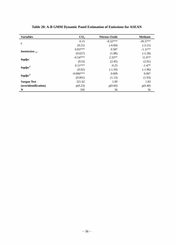
-36-
Table 20: A-B GMM Dynamic Panel Estimation of Emissions for ASEAN
Variables CO2 Nitrous Oxide Methane
c 0.15
(0.21) -8.32***
(-6.84) -30.37**
(-2.21)
lnemission t-1 0.83*** (0.027)
0.58* (1.88)
-1.11** (-2.28)
lngdpc -0.54***
(0.l3) 2.33** (2.45)
11.07* (2.01)
lngdpc2 0.11***
(0.02) -0.25
(-1.50) -1.47* (-1.96)
lngdpc3 -0.006***
(0.001) 0.009 (1.13)
0.06* (1.93)
Sargan Test (overidentification)
321.62 p(0.23)
1.00 p(0.60)
1.83 p(0.40)
N 350 36 36

-37-
Conclusions
This study examined the interaction between trade liberalization and environment in
Japan and ASEAN countries respectively employing the EKC and utilizing the panel data.
The results indicate that the region faces some environmental problems such as population
growth, increasing industrial activities, and climate change. However, the introduction of
new regulations and stricter standards, cleaner fuels, green vehicles, improving public
transportation, and promoting renewable energy are amongst measures being implemented
in the region (ASEAN, 2009). The results indicate that in carbon emissions display similar
inverted S shape when EKC is examined, such that the emission levels per capita decrease
with higher GDP in all groups. However, the turning point income levels vary depending on
the country group. Given the fact that developing countries in the region will continue to
produce and export industrial outputs, it can be expected that emission levels will still
continue in the near future. On the other hand agricultural emissions display conventional
EKC. In general the share of exports to the GDP is main contributors for carbon emission
reflecting the negative externality of export based growth. Furthermore, the trade with Japan
does not contribute to the emission levels in the region indicating that Japan does not
stimulate the pollution level in the region. FDI has a small but significant improving effect
on all groups except insignificant effect in D4. This finding demonstrates that the FDI
mostly invest in non polluting sectors in the region. However given the panel structure of the
study, country specific effects needs to be examined in the future studies. In terms of the
agricultural emissions, it can be stated that the emission levels confirm the conventional
EKC. In addition, high tariff levels increase the emission of nitrous oxide meaning that
protection leads to higher domestic production and high level of input use leading to the
pollution. On the other hand, countries with high scores in agriculture (EPI, 2009), i.e. less
subsidy and better environmental regulations, have better environmental quality in the
region. The dynamic regression indicates that the pollution of the carbon and nitrous oxide
in previous years will cause pollution in current year because of the cost of eliminating
pollution. It also shows that the dependency of economy to the polluting activities of the
related pollutants. For the case of methane, it can be said that the dependency is lower
compared to other pollutants and the methane pollution is more manageable.
The results imply that the export oriented growth in the region stimulate the
pollution, however export to Japan does not. In order to prevent the region to become
pollution havens, more strict regulations should be implemented. Given the fact that
production requires energy use and energy use per capita is an important factor in pollution
(World Bank, 2010) the region needs environmentally friendly technologies for energy
production. This can be achieved by more research and development expenditures as well as
regional collaboration. Agricultural subsidies and laxity of regulations increase the pollution

-38-
level in the region. Therefore, input related subsidies should be reconsidered and agricultural
related regulations should be implemented. In this process regional collaboration and
technical assistance and guidance are crucial for the sustainable development of the region.

-39-
References
Anderson, D. (2001). Technical Progress and Pollution Abatement: An Economic View of
Selected Technological Practices. Environment and Development Economics,
6:283-311.
Arellano, M., Bond, S. (1991). Some Tests of Specification for Panel Data: Monte Carlo
Evidence and an Application to Employment Equations, Review of Economic
Studies 58, 277-297.
ASEAN Secretariat. (2010). http://www.aseansec.org (June 15, 2010).
ASEAN (2009). Fourth ASEAN State of the Environment Report, 2009. Jakarta.
Atici, C. (2009). Carbon Emissions in Central and East Europe: Environmental Kuznets
Curve and Implications for Sustainable Development. Sustainable Development 17
(3):155-160.
Barro, R. J. Inequality and Growth in a Panel of Countries. (2000). Journal of Economic
Growth. 5(1):5-32.
Cole, M.A. (2000). Trade Liberalization, Environmental Growth and Environment.
Cheltenham: Edward Elgar.
Cole, M.A. (2003). Development, Trade, and the Environment: How Robust is the
Environmental Kuznets Curve? Environment and Development Economics. 8:557-
580.
Cole, M. A. (2004). Trade, the Pollution Haven Hypothesis and the Environmental Kuznets
Curve: Examining the Linkages. Ecological Economics 48 (1):71-81.
Comtrade (2010). http://comtrade.un.org (June 15, 2010).
Coondoo, D., Dinda, S. (2002). Causality between Income and Emission: A Country Group-
Specific Econometric Analysis. Ecological Economics. 40(3):351-367.
Copeland, B. R., and Taylor, M. S. (2004). Trade, Growth, and Environment. Journal of
Economic Literature, 42:7-71.
Dinda, S. (2004). Environmental Kuznets Curve Hypothesis: A Survey. Ecological
Economics.49 (4): 431-455.
Dobson, S., Ramlogan, C. (2009). Is There an Openness Kuznets Curve? Kyklos. 62(2):226-
238.
EPI (2010). http://epi.yale.edu (June 7, 2010).
FAO (2010).http://fao.org (June 7, 2010).
Grossman, G. M. and A. Krueger (1991). Environmental Impact of a North American Free
Trade Agreement. Working Paper 3914. NBER, Cambridge, MA.
Halkos, G.E., Tzeremes, N.G. (2010). Electricity Generation and Economic Efficiency:
Panel Data Evidence from World and East Asian Countries. Global Economic
Review. 38(3):251-263.

-40-
Halkos, G.E. (2003). Environmental Kuznets Curve for Sulfur: Evidence Using GMM
Estimation and Random Coefficient Panel Data Models. Environment and
Development Economics, 8(4):581-601.
IMF (2010). International Financial Statistics. http://www.imfstatistics.org/imf/ (June 21,
2010).
Kameyama, Y., Sari A. P., Soejachmoen, M. H. and Kanie, Norichika, Kanie, N. (2008).
Climate Change in Asia: Perspectives on the Future Climate Change. Tokyo: UN
University Press.
Kawai, Masahiro (2006). East Asian Economic Regionalism. In M. G. Plummer and E.
Jones. (eds.) International Economic Integration and Asia. New Jersey: World
Scientific.
Kuznets, S. (1955). Economic Growth and Income Inequality. American Economic Review,
45 (1):1-28.
Lee CC, Chiu, YB, Sun, CH. (2009). Does One Size Fit All? A Reexamination of the
Environmental Kuznets Curve Using the Dynamic Panel Data Approach. Review of
Agricultural Economics. 31(4):751-778.
Lee, CC., Chi, YB, Sun, C.H. (2010). The Environmental Kuznets Curve Hypothesis for
Water Pollution: Do Regions Matter? Energy Policy. 38(1):12-23.
List, J.A., Gallet, C.A. The Environmental Kuznets Curve: Does One Size Fit All?
Ecological Economics. 31(3): 409-423.
Managi, S., Kaneko, S. (2009). Environmental Performance and Returns to Pollution
Abatement in China. Ecological Economics. 68(6):1643-1651.
Markandya, A., Harou, P., Bellu, L.G., Cistulli, V. (2002). Environmental Economics for
Sustainable Growth. Cheltenham: Edward Elgar.
Matyas, L. Konya, L, Macquarie, L. (1998). The Kuznets U-curve Hypothesis: Some Panel
Data Evidence. Applied Economic Letters, 5(11): 693-697.
Mazzanti M, Montini A, Zoboli R. (2008). Environmental Kuznets Curves for Air Pollutant
Emissions in Italy: Evidence from Environmental Accounts (NAMEA) Panel Data.
Economic Systems Research.20 (3):277-301.
Munasinghe, M. (1999). Is Environmental Degradation an Inevitable Consequence of
Economic Growth: Tunneling Through the Environmental Kuznets Curve.
Ecological Economics, 29 (1): 89-109.
Muradian, R., Martinez-Alier, J. (2001). Trade and the Environment: From a Southern
Perspective. Ecological Economics. 36(2): 281-297.
Panayotu, T. (1995). Environmental Degradation at Different Stages of Economic
Development. In Beyond Rio: Environmental Crises and Sustainable Livelihoods
in the Third World. Ahmed, I. and Doeleman, J. A. (eds). ILO Studies Series, New
York: St. Martin’s Press.
Paudel, K. P., Zapata, H., and D. Susanto. (2005). An Empirical Test of Environmental

-41-
Kuznets Curve for Water Pollution. Environmental & Resource Economics, 31
(3):325-348.
Penn World Table. (2010). Center for International Comparisons of Production, Income and
Prices. http://pwt.econ.upenn.edu/ (June 29, 2010).
Perman, R., Stern, D.I. (2003). Evidence from Panel Unit Root and Cointegration Tests that
the Environmental Kuznets Curve Does not Exist. Australian Journal of
Agricultural and Resource Economics.47 (3). 325-347
Romero-Avila, D. (2008). Questioning the Empirical Basis of the Environmental Kuznets
Curve for CO2: New Evidence from a Panel Stationarity Test Robust to Multiple
Breaks and Cross-Dependence. Ecological Economics. 64 (3):559-574.
Selden, T.M., Song, D.Q. (1994). Environmental Quality and Development: Is there a
Kuznets Curve for Air Pollution Emissions. Journal of Environmental Economics
and Management. 27(2):147-162.
Shafik, N., Bandyopadhyay, S. (1992). Economic Growth and Environmental Quality: Time
Series and Cross Section Evidence. World Bank Working Paper No:904,
Washington D.C.
Shiroyama, Hideaki. (2007). Environmental Cooperation in East Asia, in T. Terao, and K.
Otsuka. Development of Environmental Policy in Japan and Asian Countries.
Eastbourne: IDE-JETRO, Palgrave Macmillan.
Soesastro, Hadi. (2008). Deepening Economic Integration in East Asia: The ASEAN
Economic Community and Beyond. ERIA Research Project Report, 2007 No: 2.
IDE-JETRO.
Suri, V., Chapman, D. (1998). Economic Growth, Trade and Energy: Implications for the
Environmental Kuznets Curve. Ecological Economics. 25:195-208
Tamazian A, Chousa JP, Vadlamannati KC. (2009). Does Higher Economic and Financial
Development Lead to Environmental Degradation: Evidence from BRIC Countries.
Energy Policy. 37(1):246-253.
Thornton, J. (2001). The Kuznets inverted-U hypothesis: Panel Data Evidence from 96
Countries. Applied Economic Letters, 8(1): 15-16.
Torras, M., Boyce, J.K. (1998). Income Inequality and Pollution: A Reassessment of the
Environmental Kuznets Curve. Ecological Economics, 25 (2):147-160.
Trade Statistics of Japan, Ministry of Finance, 2010. http://www.customs.go.jp (June 15,
2010).
UN (2010). http://unstats.un.org/unsd/snaama/dnllist.asp (June 29, 2010).
World Bank (2010). World Development Indicators. http://data.worldbank.org/indicator
(June 11, 2010).
World Bank (2010). World Wide Governance Indicators.
http://info.worldbank.org/governance/wgi/index.asp (June 30, 2010).
WTO (2006). World Tariff Profiles. Geneva, 2006.

-42-
The Author
Dr. Cemal Atici received his B.S. degree in agricultural economics from Ankara
University, Turkey. He received his M.S. degree in 1996 and Ph.D. degree in 2000 both in
agricultural economics and agribusiness from Louisiana State University. Dr. Atici is
associate professor in the department of agricultural economics at Adnan Menderes
University, Turkey. Dr. Atici’s research interests include environmental economics,
development economics, international agricultural trade, and political economy of
agricultural policies. Formerly, he carried out a research as a research fellow at Japan
International Research Center for Agricultural Sciences (JIRCAS), Tsukuba, Japan, in 2005
and at International Centre for Economic Research (ICER), Turin, Italy, in 2008. This paper
is the result of his six month stay at IDE-JETRO, Chiba, Japan from June1, 2010 to
November 25, 2010 as a Visiting Research Fellow.

-43-
List of Major Works
Atici, C. Armagan, G., Tunalioglu, R., Cinar, G. “Does Turkey’s Integration into the
European Union Boost Its Agricultural Exports?” Agribusiness: an International
Journal, 2010. (Forthcoming).
Atici, C. “Pollution without Subsidy? What is the Environmental Performance
Index Overlooking?” Ecological Economics, 68 (7), 2009:1903-1907.
Atici, C. “Carbon Emissions in Central and East Europe: Environmental Kuznets
Curve and Implications for Sustainable Development.” Sustainable Development.
2009, 17 (3):155-160.
Atici, C. and N. Doguay. “Determining the Environmental Perceptions of Cotton
Farmers in Aydin Province”. Turkish Journal of Agricultural Economics, 2009,
15(1):17-24.
Atici, C. and J. Furuya. “Regional Blocs and Agricultural Trade Flow: The Case of
ASEAN”. Japan Agricultural Research Quarterly, 42 (2), 2008:115-121.
Atici C. and F. Kurt. “Turkey’s Foreign Trade and Environmental Pollution: An
Environmental Kuznets Curve Approach”. Turkish Journal of Agricultural
Economics, 13 (2). 2008:61-69.
Atici, C. and B. Guloglu. “Gravity Model of Turkey’s Fresh and Processed Fruit
and Vegetable Export to the EU: A Panel Data Analysis.” Journal of International
Food and Agribusiness Marketing.18 (3).2006:7-22.
Atici, C. “Weight Perception and Efficiency Loss in Bilateral Trading: The Case of
US and EU Agricultural Policies.” Journal of Productivity Analysis, 24(3),
2005:283-292.
Atici, C. and P. L. Kennedy. “Tradeoffs between Income Distribution and Welfare:
The Case of Turkey's Integration into the European Union”. Journal of Policy
Modeling, 27(5), 2005:553-563.
Atici, C. “Liberalization-Goals Tradeoffs: Implications of Agricultural Trade
Liberalization for Developing Countries”. Outlook on Agriculture, 34 (2), 2005:83-
89.
Atici, C., G. Armagan, and P. Szovics. “The Competitiveness of Livestock Sector in
Some Selected European Union Candidate Countries.” Acta Oeconomica et
Informatica, 7 (2), 2004:53-56.
Atici, C. “Determining the Comparative Advantages of Cotton, Fig, and Wheat
Grown in Aydin Province.” Turkish Journal of Agricultural Economics, 7, 2002:13-
21.
Atici, C. and P.L. Kennedy. “The Impact of Turkey’s Integration into the European

-44-
Union on Agriculture in the Post Uruguay Round Environment.” Turkish Journal of
Agriculture and Forestry. 24, (4) 2000:453-456.
Kennedy, P. L. and C. Atici. A Game Theoretic Analysis of Turkish Accession to a
European Customs Union. Agricultural and Resource Economics Review. 28, (2),
1999:147-157.
Kennedy, P. L. and C. Atici. “A Sectoral Analysis of Agricultural Trade
Liberalization”. Journal of Agricultural and Applied Economics, 30, (2), 1998:277-
284.
Working Papers
Political Economy of Agricultural Policies and Environmental Weights,
International Centre for Economic Research (ICER), Working Paper Series No: 25/8,
2008.
Agricultural Policies and Environmental Interaction in OECD Countries,
International Centre for Economic Research (ICER), Working Paper Series No: 26/8,
2008.


