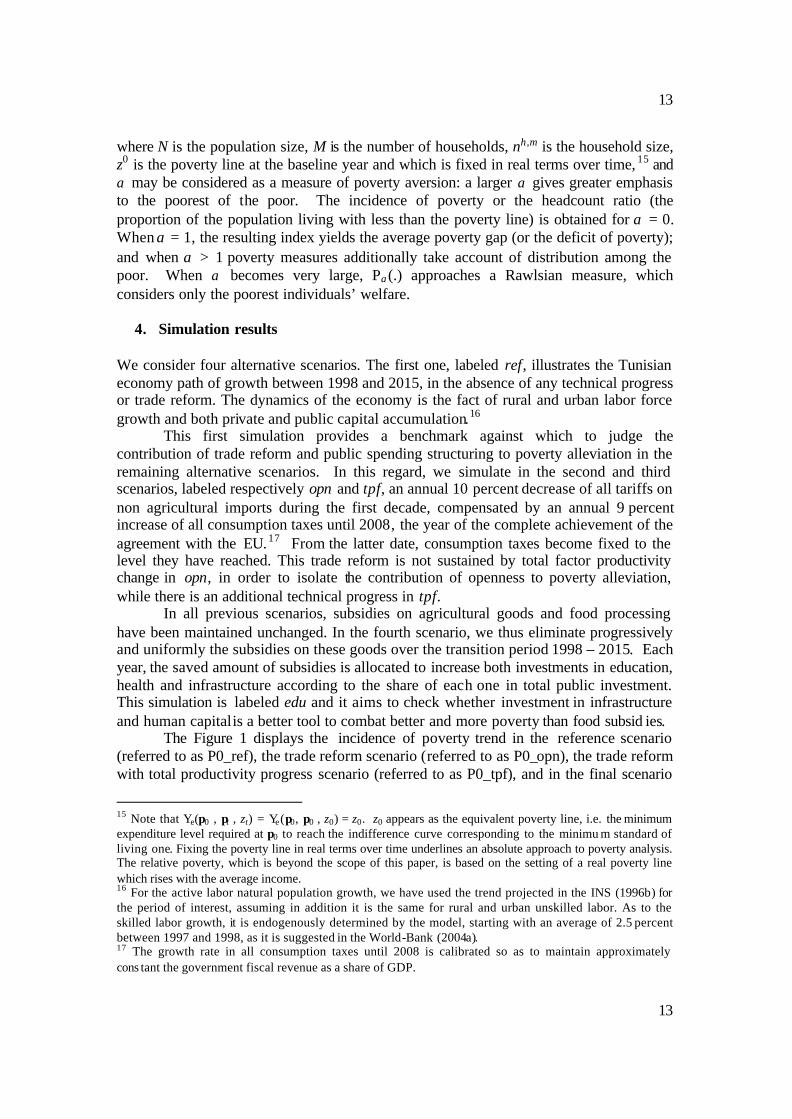
Trade Liberalization and the Dynamic of Poverty in Tunisia? A Layered CGE Microsimulation Analysis ^ Sami BIBI # and Rim CHATTI ## (Preliminary Version, June 2005) Abstract The effects of trade liberalization on poverty in Tunisia are examined, using a layered dynamic CGE- microsimulation approach. A dynamic CGE model endogenously generates the evolution of prices and, for each household group, income paths under protection and freer trade assumptions. These results are then used to assess the equivalent income of each household , using a sample from 1995 household survey, and so the effects of the simulated changes on poverty. Dominance tests are also used to avoid the arbitrariness of choosing a poverty line and a poverty measure. Simulation results show that although trade openness slowdowns the downward trend of poverty in the short and medium-run, it enhances poverty reduction in the long-run. JEL Classification : C68; I32; O24. Keywords : Trade liberalization; poverty; dynamic CGE models; sequential microsimulation; Tunisia. An early version of this paper has been presented at the conferences: “Journées AFSE-CERDI”, held in Clermont-Ferrand 19-20 May 2005, and “22 th Journées de Microéconomie Appliquée”, held in Hammamet 25-26 May 2005. The authors gratefully acknowledge financial support from FEMISE, under the project: “Analyzing the impact of trade liberalization and fiscal reforms on employment and poverty in Tunisia: An IMMPA framework”, and from API/IFPRI, under the collaborative research project: “public policy and poverty reduction in the Arab region”. They also thank Mongi Boughzala, Rachid Barouni and participants to the aforementioned conferences for their helpful comments. The usual disclaimer applies. # Associate Professor of Economics, at the Faculté des Sciences Economiques et de Gestion de Tunis (FSEGT), BP 248, El Manar, 2092, Tunis, Tunisia. Email: [email protected]; fax: +216-71-93-06-15. ## Assistant Professor of Economics, at the Ecole Supérieure des Sciences Economiques et Commerciales (ESSEC), 4 Abou Zakaria El Hafsi, 1089 Montfleury, Tunis, Tunisia. Email: [email protected].
Transcript
Trade Liberalization and the Dynamic of Poverty in Tunisia? A Layered CGE Microsimulation Analysis ⊥
Sami BIBI #
and
Rim CHATTI ##
(Preliminary Version, June 2005)
Abstract
The effects of trade liberalization on poverty in Tunisia are examined, using a layered dynamic CGE-microsimulation approach. A dynamic CGE model endogenously generates the evolution of prices and, for each household group, income paths under protection and freer trade assumptions. These results are then used to assess the equivalent income of each household , using a sample from 1995 household survey, and so the effects of the simulated changes on poverty. Dominance tests are also used to avoid the arbitrariness of choosing a poverty line and a poverty measure. Simulation results show that although trade openness slowdowns the downward trend of poverty in the short and medium-run, it enhances poverty reduction in the long-run. JEL Classification: C68; I32; O24. Keywords: Trade liberalization; poverty; dynamic CGE models; sequential microsimulation; Tunisia.
⊥ An early version of this paper has been presented at the conferences: “Journées AFSE-CERDI”, held in Clermont-Ferrand 19-20 May 2005, and “22th Journées de Microéconomie Appliquée”, held in Hammamet 25-26 May 2005. The authors gratefully acknowledge financial support from FEMISE, under the project: “Analyzing the impact of trade liberalization and fiscal reforms on employment and poverty in Tunisia: An IMMPA framework”, and from API/IFPRI, under the collaborative research project: “public policy and poverty reduction in the Arab region”. They also thank Mongi Boughzala, Rachid Barouni and participants to the aforementioned conferences for their helpful comments. The usual disclaimer applies. # Associate Professor of Economics, at the Faculté des Sciences Economiques et de Gestion de Tunis (FSEGT), BP 248, El Manar, 2092, Tunis, Tunisia. Email: [email protected]; fax: +216-71-93-06-15. ## Assistant Professor of Economics, at the Ecole Supérieure des Sciences Economiques et Commerciales (ESSEC), 4 Abou Zakaria El Hafsi, 1089 Montfleury, Tunis, Tunisia. Email: [email protected].
2
2
1. Introduction
The links between trade reform and poverty are diverse and complex. In the developing countries, the poor, i.e., households with income falling below the poverty line, share common broad features: (i) they are generally concentrated in rural (subsistence) agriculture and in urban informal sector; (ii) they have limited assets, the most abundant of which is low-skilled labor; (iii) and food is by far the most important item of their expenditure. Bo th the direct and indirect effects of trade liberalization on the poor are then to be connected with its impact on this poverty profile 1. Trade reform works directly through the transmission of price signals. Then, if it increases the price of something the poor households sell (unskilled labor, goods, services), and/or forces downward the price of something the poor household s consume (goods, services), it will increase the real income (purchasing power) of the poor households and push more poor people from below to above the poverty line, and vice versa. Economic growth is the indirect channel through which freer trade could contribute to poverty alleviation. There is now substantial empirical evidence supporting a positive association between open trade regimes and growth and development2. Indeed, trade openness reduces the anti-export bias of protection, allows efficient allocation of scarce resources and brings incentive to investment and innovation. In addition, trade reform is usually associated with higher flows of FDI with attendant spillovers of technologies, new business practices and other effects on domestic firms that increase the overall level of productivity and growth. In turn, economic growth is a powerful force for permanent and sustained poverty reduction. The extent to which growth affects poverty, however, depends on how the additional income generated by growth is distributed across the population. The more the income of the bottom segment of the population rises, the more the growth pattern is deemed to be as pro-poor. Dollar and Kraay (2002) find that the incomes of the poorest fifth of the population grew one- for-one with GDP per head in a sample of 80 countries over four decades. Trade liberalization is therefore expected to help the poor, given the positive association between openness and growth and growth and poverty reduction. However, alone trade reform is not a panacea and relying on the solely growth effect of a liberal trade policy is not sufficient to address the poverty problem. Trade liberalization should be supported by a stable macroeconomic environment and a competitive real exchange rate. Furthermore, it should be supplemented by a cocktail of other pro-poor growth policies, targeted directly towards the vulnerable segments of society. In this regard, government has an important role to play in fostering (rural) development, including through encouraging absorption of new technologies, expanding access to education, providing basic social services to poor people and investing in infrastructure.
1 A detailed synthesis of the different mechanisms through which changes in trade policy can affect the poor could be found among others in Bannister and Thugge (2001), Hoekman et al. (2001) and Winters et al. (2002). 2 Support comes from several studies including Coe et al. (1997) and Feenstra et al. (1999).
3
3
The aim of this paper is to trace through the dynamic impact of trade liberalization on the Tunisian poor, while accounting for many of the above structural features that the Tunisian poverty profile shares with the other developing countries. Indeed, trade liberalization was an integral part of the structural adjustment program that has been adopted by Tunisia since 1986. The trade policy reform has been pursued and consolidated by joining the WTO in 1990 and by concluding a FTA with the EU in 1995. The agreement called for a gradual removal of all tariff and non tariff barriers on industrial goods and the creation of a nonagricultural free-trade zone, over a twelve years transition period. It has been progressively implemented since 1996 and came into force on 1998. A complete dismantlement of these barriers on EU imports will be then achieved by 2008. In Tunisia, the large share of the work force is unskilled, having not attained the university. In 1999 for example, the distribution of employment reveals that 92.2% of the labor force is unskilled. Among them, 20.5% are working in the rural agriculture, whereas 30.7% are in the urban informal sector. As to poverty, it is mainly a rural phenomenon and to less extent urban informal in 1990, since about 65% of the poor leave in the rural area and about 10% of the poor are working in the urban informal sector.3 The extreme complexity of the linkages between trade reform and poverty motivates the use of a dynamic computable general equilibrium (DCGE) model, accounting for many of the above mentioned channels of transmission, in order to check whether the great openness of the Tunisian economy to the world market hurts the less well-off of the society. To address issues related to poverty within the framework of economy-wide models, one can identify in the literature three broad varieties of CGE methodologies. The most common method, pioneered by Adelman and Robinson (1978), consists in stratifying as much as possible the representative household into a small number of homogenous groups according to occupation, location or income criteria. Using a household income and expenditures survey, the authors assume that incomes within each group follow a lognormal distribution and then proceed to the estimation of the mean and variance of each distribution. In this approach, the CGE model provides the counterfactual change in the average income level of each of the groups, while the variance of this income and thereby the within-group inequality is assumed fixed and unaltered by the CGE experiments. Hence, changes in overall inequality can only result from a redistribution between groups, whereas analyses of household surveys indicate that changes in intra-group inequality contribute at least as much as changes in inter-group inequality to the overall disparity. Recent studies attempt to come to grip with the issue of fixed intra-group inequality by complementing CGE models with microsimulation. They can be classified into two broad categories: layered and integrated CGE-microsimulations 4. The layered CGE-microsimulation or top-down technique is conducted in two separate and sequential steps. In the first step, the CGE model is simulated to generate a full vector of commodity and factor pr ices, owing to a policy experiment. These are fed, in the second step, into a microsimulation framework which utilizes the CGE model
3 See the World Bank (1995). Note that this poverty profile would not have been changed since 1990. 4 Davies (2004) and Hertel and Reimer (2004) offer a survey of recent studies relying on these new approaches.
4
4
results on prices to conduct a detailed analysis of income distribution and poverty at the household level. This approach has two limitations. First, there is no consistency imposed between the data in the micro-simulation and the CGE models. Second, the reactions of households to commodity and factor prices changes are not (fully) transmitted back to the CGE model, so that only a fraction of the endogenous intra-group inequality is captured ; in opposition to the integrated CGE-microsimulation technique. Indeed, the latter is able to incorporate directly into a single CGE model the behavior of as many households as it is found in an income and expenditure household survey5. Although appealing, this technique needs to reconcile household data with the national data, to secure full consistency between the micro-analysis and the CGE model prediction, and this is done at the cost of restructuring households’ income or expenditures. In the present paper, we rely on the second aforementioned layered CGE-microsimulation approach to study the effect of trade liberalization on the dynamic of poverty and we suggest our own approach. In a first layer, we build a recursively DCGE model, accounting for many of the structural features of the Tunisian economy, which description is provided in section 2. The DCGE provides the resulting price and income changes from any reform over the period 1998 – 2015, which in turn will be used to communicate with the second layer microsimulation model, in a way that will be developed in section 3. Finally, section 4 exposes the consequential impact on poverty of the projected reforms and section 5 concludes.
2. DCGE model general features
The DCGE we use is deeply inspired from the (MINI)-IMMPA framework, developed by Agénor (2003) and Agénor et al. (2003). The model is calibrated to data for 1998, the latest year for which definitive information was available at sectoral level. The Tunisian economy in the reference year is desegregated into 14 production sectors, one rural agriculture and 13 urban industries and services. Except for the urban government public services, the composite output of each of the remaining 12 urban sectors results at least from one of three types of firms: private, informal, and public. They are assumed to produce imperfect substitutes in local demand. 6 The Tunisian national accounts data reveal indeed that the three types of firms do not co-exist in all sectors. Some sectors are only informal like construction, while others are only public like water and electricity. There are also sectors with both private and public or private and informal firms. Since our focus in this study is about poverty and income distribution, the household sector is disaggregated in the reference year into six household groups, identified by their source of income: two rural and four urban. Production structure
5 This approach has found application in Cogneau (1999), Cogneau and Robillard (2000), Cockburn (2001), Boccanfuso et al. (2003) and Rutherford et al. (2004). 6 The informal sector can be defined in various ways. In Tunisia, the official institute of statistics (see INS (1998)) consider as informal small sized non-agricultural firms with less than 6 employees.
5
5
Production functions in the model are of the nested form and exhibit constant returns to scale over private inputs. Gross output of all categories of firms is produced by combining in fixed proportions intermediates goods and primary factors composite. The primary factors composite is either Cobb-Douglas or CES aggregate of the various factors used in production. Indeed, we distinguish in the model four broad categories of factors: skilled and unskilled labor, land, and specific physical capital. Land is specific to the production of agriculture. In addition, physical capital is specific to the firms to which it belongs, whereas skilled and unskilled labor are treated as predetermined policy variables in the government public services sector. In addition to private inputs, it is assumed along the lines of Rioja (1999) and Kato (2002) that private and public firms as well as farmers use the economywide composite public stock of infrastructure and health, which is provided by the government, as a given external input. In this, we rely on Morrison and Schwartz (1996) and Kamps (2004) who give evidence that public capital is productive and payoffs in terms of increases in sectoral value-added and private investment. This assumption signifies that the total output of the latter firms is distrib uted entirely to the private inputs and the consideration of the return to the government from the public capital stock is ignored 7. All informal firms produce non tradable goods, as well as almost all public firms. Two exceptions for the latter categories of firms are represented by the transport and telecommunications services and mining and petroleum, since public firms are the only ones involved in export activity. The private formal firms are the main exporters in all the tradable sectors. Finally, exporting firms allocate their output to the local and international markets according to the constant elasticity of transformation aggregation. Labor market segmentation The model accounts for various sources of labor market segmentation. Unskilled workers are employed both in the rural agriculture and the urban economy. Skilled workers however are employed only in the urban formal economy. There is no unemployment in the rural region, nominal wage indeed is flexible and adjusts to clear the rural unskilled labor market. The supply of labor in the rural area is predetermined at any point in time, but grows over time at the exogenous rural population growth rate net of workers migration to urban area. Following Harris and Todaro (1970), the incentive to migrate is taken to depend negatively on the ratio of the expected real wage in rural area to that prevailing in urban area. Unskilled workers in the urban economy may be employed either in the informal, private, or public enterprises. In the formal activities, it is assumed along the lines of Kheo et al. (1995), that unions fix the uniform unskilled (skilled) labor real wage. The latter depends negatively on the unskilled (skilled) labor unemployment. It is also assumed that the wage rate of unskilled (skilled) labor is equal in the private and public enterprises, and it is greater than that paid in the informal sector. This gives an incentive to unskilled workers to seek a job in the private and public enterprises first. The total supply of unskilled workers in the formal sector is allowed to adjust over time according to the expected wage differential between the informal and formal 7 In this we depart from the (MINI)-IMMPA framework, which considers the public capital as an internal input of production.
6
6
sectors. The total supply of unskilled workers in the informal labor market is instead determined residually and it always equals the induced demand for unskilled labor by all informal enterprises. The wage in the informal market is therefore uniform and flexible. The supply of unskilled labor in the urban sector evolves as a result of (exogenous) natural urban populatio n growth and migration of unskilled labor from the rural economy. Moreover, given the skilled and unskilled wage differential and the public capital stock of education per capita, some urban unskilled workers become skilled and leave the unskilled workforce to increase the supply of skilled labor. Skilled workers who are unable to find a job in the formal economy opt to remain openly unemployed, instead of entering the informal economy, and the progress of the skilled labor force supply depends on the rate at which unskilled workers acquire skills. The distribution of unskilled employment in the reference year reveals that the rural agriculture and the urban informal sector provide together 51.2 percent of unskilled labor employment, whereas each of the public and private sectors offers around 16 percent of unskilled jobs. As a consequence of this unskilled job distribution, 16.8 percent of the unskilled workforce is unemployed in the reference year. Job provision for skilled workers in 1999 is such that the public sector is the main sector creating jobs for the more-educated workers, as it employs 82 percent of the skilled workforce in the base year.8 Government administration accounts for 91 percent of total public sector skilled labor employment, whilst public enterprises account for the remaining 9 percent. Compared to public sector, private sector absorbs only 8.7 percent of the skilled workforce. Since the agriculture and informal sectors do not rely on skilled work in their production process, the remaining 8.6 percent of the skilled find themselves without a job.9 This figure shows that the public sector plays an important role in skilled labor policy for the economy as a whole. More details about the distribution of labor between the different sectors and firms could be found in Table 1. Demand structure Producers demand composite goods, imported and local, for intermediate use, according to a Leontief input-output technology; that is, the coefficients of intermediate goods in production are fixed. The model furthermore explicitly features the expenditures flows arising from government behavior and the activities of private investors. It is assumed that both government expenditures, saving and transfers to households are in fixed proportion of its revenue. Government expenditures consist of current unproductive expenditures as well as productive public investment. It is also made in the model a distinction between the investments in infrastructure, education and health. In 1998, the public investment in infrastructure accounts for 1.7 percent of current
8 Although we use a 1998 SAM, we rely on information form the 1999 population census to allocate all the labor force between sectors and firms. 9 In reality, the agriculture and the informal sector employ very small shares of the skilled workforce, 0.1 percent in agriculture (see INS (2002b)) and 0.4 percent in the informal sector (see INS (1998)). Since the distribution of wages between skilled and unskilled was not available, we have considered that these two sectors are not relying on skilled work.
7
7
GDP, whereas public investments in health and education represent respectively 0.3 percent and 1 percent of GDP.
8
8
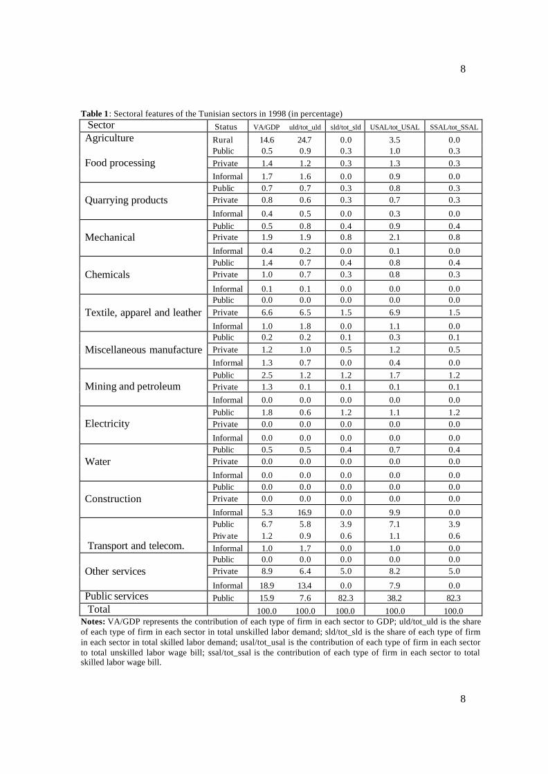
Table 1: Sectoral features of the Tunisian sectors in 1998 (in percentage) Sector Status VA/GDP uld/tot_uld sld/tot_sld USAL/tot_USAL SSAL/tot_SSAL
Transport and telecom. Informal 1.0 1.7 0.0 1.0 0.0 Public 0.0 0.0 0.0 0.0 0.0 Private 8.9 6.4 5.0 8.2 5.0
Other services Informal 18.9 13.4 0.0 7.9 0.0 Public services Public 15.9 7.6 82.3 38.2 82.3 Total 100.0 100.0 100.0 100.0 100.0
Notes: VA/GDP represents the contribution of each type of firm in each sector to GDP; uld/tot_uld is the share of each type of firm in each sector in total unskilled labor demand; sld/tot_sld is the share of each type of firm in each sector in total skilled labor demand; usal/tot_usal is the contribution of each type of firm in each sector to total unskilled labor wage bill; ssal/tot_ssal is the contribution of each type of firm in each sector to total skilled labor wage bill.
9
9
Each distinguished type of public investment allows the endogenous accumulation of the corresponding public capital stock. The accumulation process is modeled in a conventional way, where the next period stock of each public capital stock is equal to the amount invested in the current period plus the surviving stock. We further assume geometric depreciation that is, the capital stock depreciates at a constant rate. The public stock in education affects positively the skills formation, whereas the public stock of infrastructure has, in one hand, a positive effect on private investment and, in the other hand, combines with the public stock of health to increase the total factor productivity in agriculture, public and private firms, as above explained. Following, the World Bank (1996) estimations for Tunisia, an increase in public investment or government spending on education as a share of GDP by 1 percentage point would enhance the per capita GDP growth by 0.2 percent. Furthermore, a rise in the ratio of government consumption net of education spending to GDP by 1 percentage point would reduce the per capita GDP growth by 0.12 percent. Finally, an expansion of the share of exports in GDP by 1 percentage point would contribute to the augmentation of the per capita GDP by 0.06 percent. Adding the population growth rate to these estimates, we obtain an approximate of the impact of these changes on the total factor productivity. Thus, we have taken the latter estimates of the determinants of productivity explicitly into consideration in addition to the productive contribution of the public stock in infrastructure and health. It is assumed that they affect simultaneously the shift parameter in the production function of agriculture, public and private firms. It is also assumed that the contribution of the change in the ratios of infrastructure and health expenditures to GDP is equal to that of education spending. The government revenue derives from the transferred returns on capital of public firms and from the collection of taxes on revenues, tariffs and consumption. In the base year, 30 percent of the government fiscal revenue is driven from tariffs on imports and 34.2 percent from consumption taxes, whereas the contribution of households’ income and corporate taxation to total fiscal revenue are respectively equal to 21.8 and 14.1 percent. This fiscal structure allows the government to reap 25 percent of the 1998 GDP. The investment demand for the different composite goods by sector of origin are also assumed to be in fixed shares of total investment demand, which is equal to total saving. Capital accumulation is assumed to occur only in the urban private firms, according to the same conventional process as the public capital stock accumulation. The decision to invest hinges positively on the after tax rate of return to capital relative to cost of funds and on the public capital stock in infrastructure as well as the real GDP change. As already mentioned, the model identifies six household types grouped by socio-economic status and labeled by h, h=1,6. The landholders in agriculture and the agricultural workers represent two distinct households living in the rural area. The remaining four urban households are the unskilled households working in the informal enterprises, the unskilled employees working both in the formal private and public sectors, the skilled households working in the formal private and public sectors and the capitalists. Classifying households groups in this way allows the model to identify the impact of economic reforms on income distribution and poverty. Household revenue is based on salaries and/or distributed profits, in addition to government and ROW
10
10
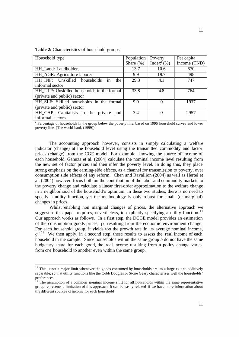
transfers. Table 2 sets out the characteristics of each group, including shares of population, per capita income, and poverty index. Households’ preferences are represented by Cobb-Douglas utility indices defined over saving and the 14 composite goods. Saving and demands are so a constant fraction of households’ after tax revenue. Each composite consumption good is then a sum of households groups, government and investors final consumption demands and all producers’ intermediate composite goods demands. It is also assumed to be a CES aggregation of imported and composite domestic goods. The latter are deemed to be imperfect substitutes by the local demanders. Furthermore, it is assumed that the composite domestic good is a CES aggregation of informal, private and public domestic goods. The above DCGE model, which formal description is given in annex, is designed in a way to capture the relevant structural features of the Tunisian economy, in order the price and income changes it generates embody both the effective direct and indirect effects of the policy reform and the attribution of these changes to the reform are unambiguous. In this way, any change of poverty obtained from the microsimulation model, which we describe in the subsequent section, will be as close as possible to what would be expected.
3. An Overview of the Microsimulation Approach Incorporating directly into a DCGE model as many households as there are in a household survey would be certainly the ideal approach to address the question of the dynamics of poverty following any economic change. This is indeed the best way to keep all the information about the households’ heterogeneity with regards to their pattern of endowment and consumption. Unfortunately, the Tunisian household expenditures survey is notable for its under-reporting of the source and level of each household member’s income and its composition. The relevant information it records for our purpose is the households’ expenditures for various items, the household’s head level of education and occupation. The latter information is used to roughly decompose, not without making some assumptions, the available sample of 2500 households from the 1995 household survey into the closest six groups in the DCGE model. 10 The aim is to proceed to a layered CGE-microsimulation analysis. As pointed out by Ganuza et al. (2004), in the top-down methodology, microsimulations range from pure accounting approaches to models with behavioral equations based on econometric estimates. The seminal work by Bourguignon et al. (2003) falls in the latter category. The authors indeed estimate the microsimulation model which is based on a set of equations representing a detailed description of the real income generation mechanism at the household level. The estimated model captures the heterogeneity of households in terms of income sources, area of residence, endowment in human capital and consumption preferences.
10 The 1995 household survey is multipurpose and provides reliable information on consumption expenditures on many commodities and extensive socio-demographic information on about 10000 households. The survey does not include, however, information on incomes leading to the use of total household expenditure per capita for characterizing the dynamics of poverty.
11
11
Table 2: Characteristics of household groups
Household type Population Share (%)
Poverty Indexa (%)
Per capita income (TND)
HH_Land: Landholders 13.7 10.6 670 HH_AGR: Agriculture laborer 9.9 19.7 498 HH_INF: Unskilled households in the informal sector
29.3 4.1 747
HH_ULF: Unskilled households in the formal (private and public) sector
33.8 4.8 764
HH_SLF: Skilled households in the formal (private and public) sector
9.9 0 1937
HH_CAP: Capitalists in the private and informal sectors
3.4 0 2957
a Percentage of households in the group below the poverty line, based on 1995 household survey and lower poverty line (The world-bank (1999)). The accounting approach however, consists in simply calculating a welfare indicator (change) at the household level using the transmitted commodity and factor prices (change) from the CGE model. For example, knowing the source of income of each household, Ganuza et al. (2004) calculate the nominal income level resulting from the new set of factor prices and then infer the poverty level. In doing this, they place strong emphasis on the earning-side effects, as a channel for transmission to poverty, over consumption side effects of any reform. Chen and Ravallion (2004) as well as Hertel et al. (2004) however, focus both on the contribution of the labor and commodity markets to the poverty change and calculate a linear first-order approximation to the welfare change in a neighborhood of the household’s optimum. In these two studies, there is no need to specify a utility function, yet the methodology is only robust for small (or marginal) changes in prices. Whilst enabling non marginal changes of prices, the alternative approach we suggest in this paper requires, nevertheless, to explicitly specifying a utility function.11 Our approach works as follows. In a first step, the DCGE model provides an estimation of the consumption goods prices, pt, resulting from the economic environment change. For each household group, it yields too the growth rate in its average nominal income, gt
h.12 We then apply, in a second step, these results to assess the real income of each household in the sample. Since households within the same group h do not have the same budgetary share for each good, the real income resulting from a policy change varies from one household to another even within the same group.
11 This is not a major limit whenever the goods consumed by households are, to a large extent, additively separable; so that utility functions like the Cobb Douglas or Stone Geary characterizes well the households’ preferences. 12 The assumption of a common nominal income shift for all households within the same representative group represents a limitation of this approach. It can be easily relaxed if we have more information about the different sources of income for each household.
12
12
More precisely, we assume that each household m within a group h has an original income per capita Y0
h,m and faces the price system p0 in the baseline year. From one year to the other, each household in the sample faces a new vector of prices and income (pt,Yt
h,m). Since we aim to compare the levels of an individual's welfare over time, we consider the baseline price vector (p0) as the reference price system.13 Then, we define as King (1983) the concept of equivalent income: for a given budget constraint (pt, Yt), the equivalent income is defined as that income level which allows, at p0, the same utility level as can be reached under the given budget constraint. Formally, we have:
),()),,(,( 00 tttte YvYYv pppp = (1) where v(.) is the indirect utility function, pt is a vector of price system at t, and Yt is the per capita household ’s nominal income. Notice that since p0 is fixed across all households, Ye(.) is an exact monetary metric of actual utility v(pt, Yt) because Ye(.) is an increasing monotonic transformation of v(.). Thus, inverting the indirect utility function, we obtain the equivalent income, Ye(p0, pt, Yt). We take the predicted price and income changes from the DCGE model as given for the analysis of welfare impacts at the household level. Since we assume that the growth rate within each household group is the same for all households belonging to the same group and equal to gt
h, we have : mhh
tmh
t YgY ,0
, )1( += (2) By (2), and assuming a Cobb-Douglas utility function, we can compute the indirect utility function, v(.) for each household in the sample using this formula:
∏+
==
I
i
mhkw
timhht
mhtt p
YgYv
1
,
,,0
, )()1(
1),(p (3)
where pi,t is the price of good i at the period t and wih,m is the budget share devoted to the
good i by the household m within the group h. Using (1) and (3), the equivalent income of each household in the sample at each period t is then given by:
∏ +
=
=
I
i
mhht
mhiw
ti
imhtte Yg
pp
YY1
,0
,
,
0,,0 )1(),,( pp (4)
Further to information about the distribution of equivalent income among households, it is worthy to assess the social impact of the change. A natural measure could be given by the variation of a pre-specified poverty yardstick. An important class of poverty measures is the FGT class of additively decomposable indices suggested by Foster et al. (1984), which can be written in terms of equivalent income as:14
( )( )∑ +−=
∑
+−=Ρ
=+
=+
M
m
mhhtte
mh
M
m
mhhttemht
et
ygynN
zYgY
nN
yz
1
,00
,
1 0
,00,
0
)1(,,11
))1(,,(1
1),(
α
α
α
pp
pp
(5)
13 Following King (1983), the choice of the reference price system is to some extent arbitrary, although for the analysis based on computable general equilibrium models, the baseline price vector, p0, is a natural choice. The reason for this is that any comparison must use a common reference price system. 14 Writing poverty measures in terms of equivalent income make them sensitive to both income and prices variations.
13
13
where N is the population size, M is the number of households, nh,m is the household size, z0 is the poverty line at the baseline year and which is fixed in real terms over time, 15 and α may be considered as a measure of poverty aversion: a larger α gives greater emphasis to the poorest of the poor. The incidence of poverty or the headcount ratio (the proportion of the population living with less than the poverty line) is obtained for α = 0. When α = 1, the resulting index yields the average poverty gap (or the deficit of poverty); and when α > 1 poverty measures additionally take account of distribution among the poor. When α becomes very large, Ρα(.) approaches a Rawlsian measure, which considers only the poorest individuals’ welfare.
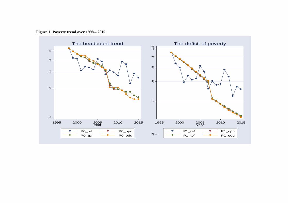
4. Simulation results We consider four alternative scenarios. The first one, labeled ref, illustrates the Tunisian economy path of growth between 1998 and 2015, in the absence of any technical progress or trade reform. The dynamics of the economy is the fact of rural and urban labor force growth and both private and public capital accumulation.16 This first simulation provides a benchmark against which to judge the contribution of trade reform and public spending structuring to poverty alleviation in the remaining alternative scenarios. In this regard, we simulate in the second and third scenarios, labeled respectively opn and tpf, an annual 10 percent decrease of all tariffs on non agricultural imports during the first decade, compensated by an annual 9 percent increase of all consumption taxes until 2008, the year of the complete achievement of the agreement with the EU.17 From the latter date, consumption taxes become fixed to the level they have reached. This trade reform is not sustained by total factor productivity change in opn, in order to isolate the contribution of openness to poverty alleviation, while there is an additional technical progress in tpf. In all previous scenarios, subsidies on agricultural goods and food processing have been maintained unchanged. In the fourth scenario, we thus eliminate progressively and uniformly the subsidies on these goods over the transition period 1998 – 2015. Each year, the saved amount of subsidies is allocated to increase both investments in education, health and infrastructure according to the share of each one in total public investment. This simulation is labeled edu and it aims to check whether investment in infrastructure and human capital is a better tool to combat better and more poverty than food subsid ies. The Figure 1 displays the incidence of poverty trend in the reference scenario (referred to as P0_ref), the trade reform scenario (referred to as P0_opn), the trade reform with total productivity progress scenario (referred to as P0_tpf), and in the final scenario
15 Note that Ye(p0 , pt , zt) = Ye(p0, p0 , z0) = z0. z0 appears as the equivalent poverty line, i.e. the minimum expenditure level required at p0 to reach the indifference curve corresponding to the minimu m standard of living one. Fixing the poverty line in real terms over time underlines an absolute approach to poverty analysis. The relative poverty, which is beyond the scope of this paper, is based on the setting of a real poverty line which rises with the average income. 16 For the active labor natural population growth, we have used the trend projected in the INS (1996b) for the period of interest, assuming in addition it is the same for rural and urban unskilled labor. As to the skilled labor growth, it is endogenously determined by the model, starting with an average of 2.5 percent between 1997 and 1998, as it is suggested in the World-Bank (2004a). 17 The growth rate in all consumption taxes until 2008 is calibrated so as to maintain approximately cons tant the government fiscal revenue as a share of GDP.
14
14
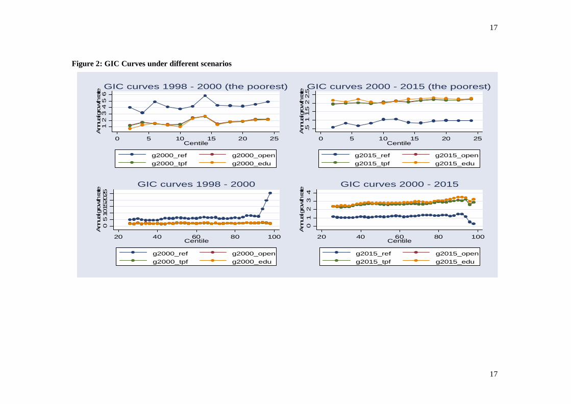
when the saving from food subsid ies removal are used to enhance investment in education, health and infrastructure (referred to as P0_edu). The left-hand side of this figure displays the headcount ratio trend under these different scenarios. Interestingly enough, trade liberalisation and food subsidy removal appear to be not pro-poor in the short run but really pro-poor in the long run. Indeed, the left-hand side of Figure 1 shows that until 2005 (and even until 2008, the year of the complete achievement of tariffs dismantlement), the simulated reforms and mainly the one where subsidies are removed would push up the downward trend of poverty. Yet, from 2008 onwards, the substitution of public investment to food subsid ies would contribute most to the achievement of the Millennium Development Goal of halving poverty, as measured by the headcount ratio, by 2015. Indeed, while more than 5 percent of the population are in extreme poverty in 1998, by 2015 less than 2 percent of the population would remain in extreme poverty under the last scenario. The headcount ratio could fail to accurately capture the impact of any change on poverty, indeed it only records those who escape or reach the segment of the poor. Thus, it could under-estimate the effectiveness of the other reforms, since most poor people could find their welfare improved but not enough to lift poverty. To curb this likely drawback, the right-hand side of Figure 1 displays the estimates of the poverty deficit, Ρ1(.), during the period under consideration resulting from the different changes. These curves show similar decreasing trend as the poverty incidence, meaning that the average income of those staying below the poverty line has increased. Further, from 2008 to 2015, the poverty deficit curve resulting from the elimination of subsidies will lie always below the others. The above analysis could depend critically on the choice of the poverty line and poverty measures. Since both of these choices are somewhat arbitrary, so could be the dynamics of poverty characterised using the m. Drawing on the recent study of Ravallion and Chen (2003), it is fortunately possible to curb such degrees of arbitrariness by computing first the growth rate in the mean of each income quantile:
1)(
)()(
1−=
− qy
qyqg
te
te (6)
where g(q) is the growth rate in the King’s (1983) equivalent income of the qth quantile between t and t-1 and yt
e(q) is the mean of ye(p0, pt, yt) within the quantile q at the pertinent period.18 Considering the full range of possible q, g(q) traces out the growth incidence curve (henceforth GIC curve), showing how the growth rate is distributed across different quantiles, ranked by equivalent income. Figure 2 splits the period of transition in two: one going from 1998 to 2000 and the other from 2000 to 2015. For each period, we give the average income rate of growth of the 25 percent least endowed individuals and the remaining segments of the society, under the different reforms. The top left and right sides of Figure 2 show that the GIC curves lie nowhere below 0, meaning that poverty will certainly fall within the period under consideration, regardless of the chosen poverty line and the poverty measure. In the stochastic dominance literature, this finding is known as “first-order dominance” (FOD).19
18 Alternatively, ye(q) could be expressed as ye(p0, pt, yt(q)). 19 See, among many others, Atkinson (1987) for a detailed description on the stochastic dominance tests.
15
15
The same graphs show that in the first period, the income growth pattern of the poorest is the lowest under food subsidies removal reform (referred to as g2000_edu), while it becomes the highest within the same scenario in the second period, once the indirect effect of investment in infrastructure and human capital begins to bear fruit to the poor. The right-hand side of Figure 2 also shows that from 2000 to 2015, the trade reform improves the equivalent income of all the individuals. However, the total productivity progress (referred to as g2015_tpf) considered in addition to openness reform (referred to as g2015_opn) adds roughly nothing to the gains achieved through better allocation of scarce resources, since the two GIC curves are very close. As to the reform of subsidies program (referred to as g2015_edu), it even boosts the gains obtained from trade liberalization. Finally, all the GIC curves displayed in Figure 2 do not switch sign. Then there is no need to test higher order dominance to study less robustly the dynamics of poverty.20 Testing solely FOD conditions is not yet really informative about the distributional pattern of economic growth. For instance, the GIC curves displayed in the left-hand side of Figure 2 are approximately horizontal. This means that the Lorenz curve does not really shift at the beginning period under consideration, and the economic growth is to some extent, distribution-neutral. Nevertheless, the right-hand side of Figure 2 shows that g(q) exhibits an upward sloping across different income quantiles. Thus, while curbing absolute poverty, this growth pattern will worsen all inequality measures, and then relative poverty, since the richest quantiles profit more from economic growth than the poorest ones.
20 On the higher dominance tests about the link between economic growth and poverty, see for instance Son (2004) and Bibi (2005) .
Figure 1: Poverty trend over 1998 – 2015
12
34
5
1995 2000 2005 2010 2015year
P0_ref P0_opn
P0_tpf P0_edu
The headcount trend
.2.4
.6.8
11.2
1995 2000 2005 2010 2015year
P1_ref P1_opn
P1_tpf P1_edu
The deficit of poverty
17
17
Figure 2: GIC Curves under different scenarios
12
34
56
Ann
ual g
row
th ra
te
0 5 10 15 20 25Centile
g2000_ref g2000_open
g2000_tpf g2000_edu
GIC curves 1998 - 2000 (the poorest)
.51
1.5
22.5
Ann
ual g
row
th ra
te
0 5 10 15 20 25Centile
g2015_ref g2015_open
g2015_tpf g2015_edu
GIC curves 2000 - 2015 (the poorest)
05
1015
2025
Ann
ual g
row
th ra
te
20 40 60 80 100Centile
g2000_ref g2000_open
g2000_tpf g2000_edu
GIC curves 1998 - 2000
01
23
4Ann
ual g
row
th ra
te
20 40 60 80 100Centile
g2015_ref g2015_open
g2015_tpf g2015_edu
GIC curves 2000 - 2015
18
18
5. Conclusion In this paper, a DCGE model is used to assess the impact of trade liberalization on poverty in Tunisia. To achieve this goal, it was common in the literature to classify foremost households according to some socio -economic grouping. Then, a distribution function (usually a log-normal distribution) for each household group is constructed in order to describe the variation of income distribution and poverty following a policy change. The main drawback of such approach is that the intra-group variances are specified exogenously. Therefore, this type of models will not capture the within-group variation of inequality (following a policy change) which represents generally a large share of the overall change of inequality. This would provide a biased estimation of poverty change, essentially when the poverty indices used are sensitive to the distribution of the well-being within the poor. The alternative route is to include all households from a survey directly in to the CGE model. However, the lack of the relevant information on the (source of) revenue in the Tunisian household survey impedes us to proceed to an integrated microsimulation. We instead limit ourselves to layered microsimulation, which captures a (good) fraction of the within-group variation of inequality, in addition to the between-group variation of inequality. In this regard, we infer the prices change and the variation rate of each household income group provided by the DCGE simulation change into the households of the survey, previously classified by groups, to assess the equivalent income of each one. Since households do not have the same budgetary share for each good, the equivalent gain (or loss) varies from a household to another even within the same group. This enables a better characterization of poverty change within each group and has several policy implications in terms of the choice of groups that should benefit from an anti-poverty program and the cost of such program. The empirical illustration of this methodology computes the likely effects of trade liberalization and more public investment on infrastructure and human capital financed by food subsidy removal. The main results are outstanding, showing that such changes could slowdown the poverty reduction in the short run, but enhance it in the long run. The present study is mainly illustrative. The analysis of the effects of trade liberalization on income distribution and poverty requires more detailed information. For instance, earnings and occupational choice of households’ head should be modeled as a function of their specific characteristics. Thus, whenever there is a change in the aggregate demand for wage labor, which workers move from the formal to the informal sector (and reciprocally) depends on their specific characteristics. Such a shift can be at the root of a significant change in income distribution and poverty. Capturing these effects requires, nevertheless, that our methodology should be supplemented by an econometric model which characterizes the households’ labor market responses to external shocks. Although such characterization is needed to improve the predictive power of any layered microsimulation framework, it is precluded by data availability for the present study. However, the outcome of this analysis highlights the potential return from a more refined research that could provide guidelines for policymakers on the optimal level of any change as well as its expected effects.
19
19
References Adelman, I. and S. Robinson (1978). Income Distribution and Growth; A Case Study of Korea, Oxford University Press: Oxford. Agénor, P. R. (2003) Mini-IMMPA: A Framework for Analyzing the Unemployment and Poverty Effects of Fiscal and Labor Market Reforms. The World -Bank, May. Agénor, P. R., D. H. C. Chen and M. Grimm (2003) Linking Representative Household Models with Household Surveys for Poverty Analysis: A Comparison of Alternative Methodologies. The World Bank, December. Atkinson, A. B. (1987). On the Measurement of Poverty. Econometrice, vol. Bannister, G. J. and K. Thugge (2001) International Trade and Poverty Alleviation. The IMF working Paper 01/54, May. Bibi, S. (2005) When is Economic Growth Pro-poor? Evidence from Tunisia. Mimeo. Boccanfuso, D., B. Decaluwe and L. Savard (2003). ‘Poverty, Income Distribution and CGE Modelling: Does the Functional Form of Distribution Matter?’, CIRPEE, Universite Laval: Quebec. Bourguignon, F., A.-S. Robilliard and S. Robinson (2003) Representative Versus Real Households in the Macroeconomic Modelling of Inequality, DIAL Working Paper DT/2003-10, Paris. Chen, S. and M. Ravallion (2004) Welfare Impacts of China’s Accession to the WTO. World Bank Economic Review 18: 29–57. Cockburn, J. (2001) Trade Liberalization and Poverty in Nepal: A Computable General Equilibrium Micro Simulation Analysis, CREFA Discussion Paper 01-18, CREFA, Université Laval: Quebec. Coe, D., E. Helpman and E. Hoffmaister (1997) North-South R&D Spillovers. The Economic Journal 107: 134–149. Cogneau, D. (1999) Labour Market, Income Distribution and Poverty in Antananarivo: A General Equilibrium Simulation (mimeo), DIAL: Paris. Cogneau, D. and A.-S. Robilliard (2000) Growth, Distribution and Poverty in Madagascar: Learning from a Microsimulation Model in a General Equilibrium Framework, TMD Discussion Paper No. 61, International Food Policy Research Institute: Washington DC. Davies, J. B. (2004) Microsimulation, CGE and Macro Modelling for Transistion and Developing Economies, World Institute for Development Economics Research Discussion Paper No. 2004/08. Dollar, D. and A. Kraay (2002) Growth is Good for the Poor. Journal of Economic Growth, vol. 7, pp. 195 – 225. Feenstra, R., D. Madani, T. H. Yang and C. Y. Liang (1999) Testing Endogenous Growth in South Korea and Taiwan. Journal of Development Economics 60: 317–341. Foster, J. E., J. Greer and E. Thorbecke (1984), A Class of Decomposable Poverty Measures. Econometrica, 52(3): 761−765. Ganuza, E., S. Morley, S. Robinson, V. Pineiro and R. Vos (2004) Are Export Promotion and Trade Liberalization Good for Latin America’s Poor? A Comparative Macro- Micro CGE Analysis. In S. Robinson and R. Vos Eds., Is Trade Liberalization Good for Latin America’s Poor?, UNDP. Harris, J. and M. Todaro (1970) Migration Unemployment and Development: A Two- Sector Analysis. American Economic Review, 60: 126–142.
20
20
Hertel, T.W., M. Ivanic, P. V. Preckel and J. A. L. Cranfield (2004) The Earnings Effects of Multilateral Trade Liberalization: Implications for Poverty, World Bank Economic Review 18: 205–236. Hertel, T. W. and J. J. Reimer (2004) Predicting the Poverty Impacts of Trade Reform. World Bank Policy Research Working Paper 3444, November. Heokman, B., C. Michalopoulos, M. Schiff and D. Tarr (2001) Trade Policy Reform and Poverty Alleviation, Policy Research Working Paper N. 2733, The Worldbank. Institut National de la Statistique (1996a) Recensement Général de la Population et de l’Habitat en 1994 : Caractéristique Economiques Institut National de la Statistique (1996) de la Population. Institut National de la Statistique (1996b) Projections de la Population Active et de la Demande Additionnelle d’Emplois : 1995–2015. Institut National de la Statistique (1998) Les Micro-Entreprises en 1997. Institut National de la Statistique (2002a) Rapport Annuel sur les Caractéristiques et les salaires des Agents de la Fonction Publique. Institut National de la Statistique (2002b) Recensement Général de la Population et de l’Emploi en 1999. Kamps, C. (2004) The Dynamic Macroeconomic Effects of Public Capital: Theory and Evidence for OECD Countries. Kiel Studies 331. Springer. Kato, R. R. (2002) Government Deficit, Public Investment, and Public Capital in the Transition to an Aging Japan. Journal of the Japanese and International Economies vol.16, pp. 462–491. Kheo, T. J., C. Polo and F. Sancho (1995) An Evaluation of the Performance of an Applied General Equilibrium Model of the Spanish Economy. Economic Theory, 6: 115−141. King, M. A. (1983), Welfare Analysis of Tax Reforms using Household Data. Journal of Public Economics, 21: 183−214. Morrison, C. J. and A. E. Schwartz (1996) State Infrastructure and Productive Performance. The American Economic Review vol. 86 (5), pp. 1095–1111. Ravallion, M. (1998), Poverty Lines in Theory and Practice. Unpublished Paper. The World Bank. Ravallion, M. and S. Chen (2003) Measuring Pro-Poor Growth. Economics Letters, vol. 78, pp. 93– 99. Rioja, F. K. (1999) Productiveness and Welfare Implications of Public Infrastructure: a Dynamic Two-Sector General Equilibrium Analysis. Journal of Development Economics vol. 58, pp. 387– 404. Rutherford, T. D. Tarr and O. Shepotylo (2004) Household and Poverty Effects from Russia’s Accession to the WTO. Paper Presented at the Empirical Trade Analysis Conference, Woodrow Wilson Center, Washington, D.C., January 22–23. Winters, A., N. McCulloch and A. McKay (2002) Trade Liberalization and Poverty: The Empirical Evidence. University of Sussex Discussion Paper in Economics 88, October. World Bank (1996) Tunisia’s Global Integration and Sustainable Development: Strategic Choices for the 21st Century. International Bank for Reconstruction and Development, Washington, D. C., august 1996.
21
21
World Bank (1999), République Tunisienne, Revue Sociale et Structurelle, Groupe du Développement Economique et Social, Région Moyen-Orient et Afrique du Nord. World Bank (2004) Republic of Tunisia Employment Strategy: Volumes I and II. May. World Bank (2004) Republic of Tunisia Development Policy Review: Making Deeper Trade Integration Work for Growth and Jobs. October.
22
22
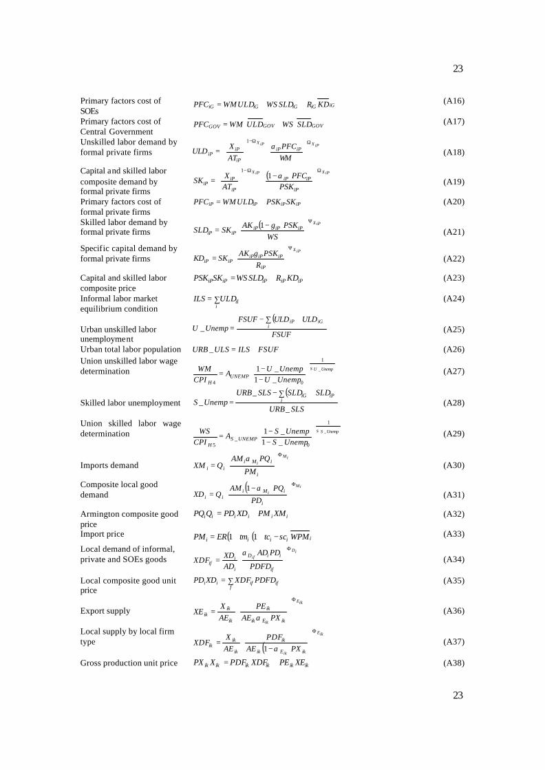
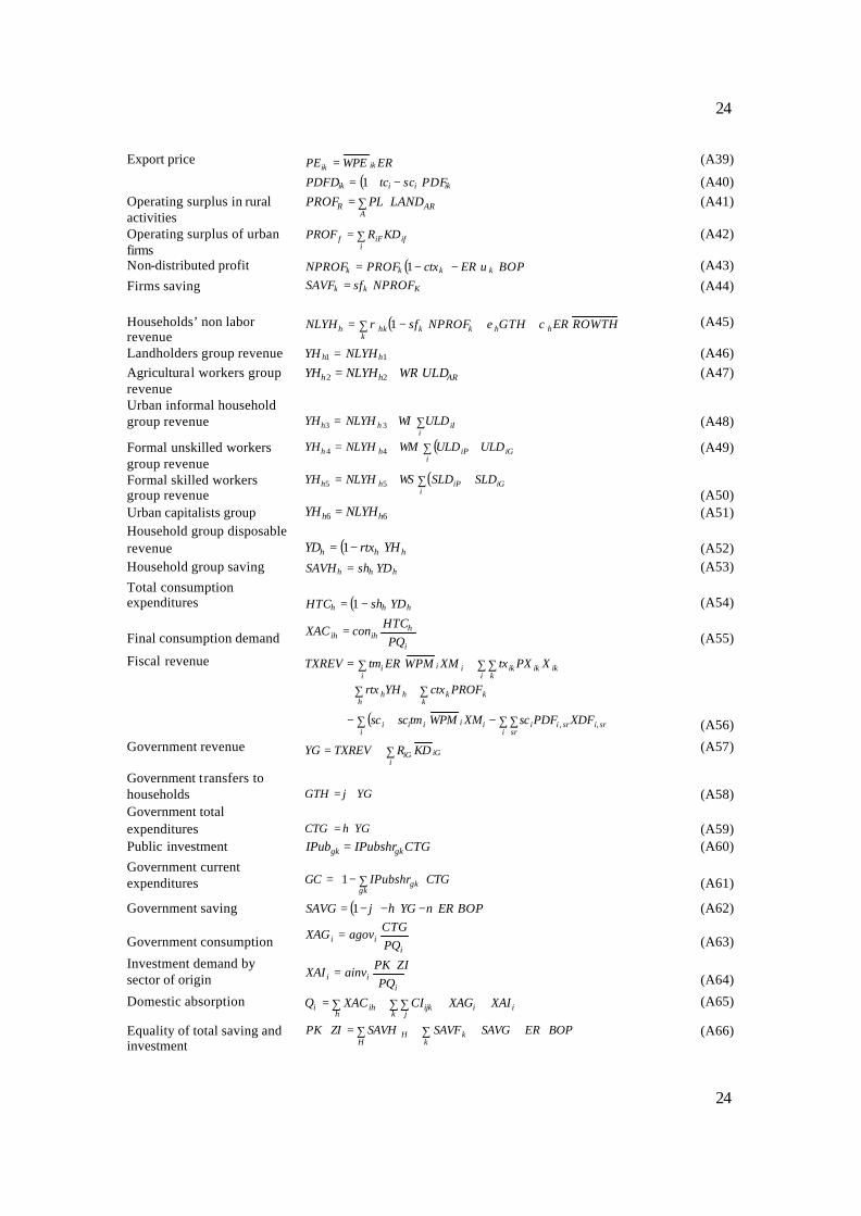
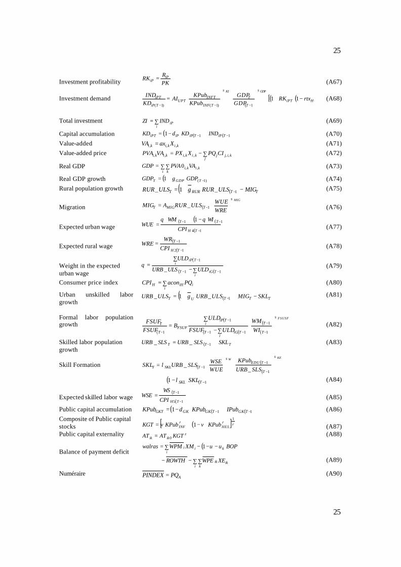
Appendix: Model Equations
i,j=A(agriculture),2-14; k = R(rural), I(informal), P(private), G(public); f = I, P, G; gk =
INF(infrastructure), EDU(education), HEL(health); H = H1-H6
Public capital accumulation ( ) ( ) ( )111 −− +−= TGKTGKGKGKT IPubKPubKPub δ (A86) Composite of Public capital stocks ( )[ ] ρρρ ϖϖ
1
1 HELINF KPubKPubKGT −+=
(A87) Public capital externality ζKGTATAT ikik 0= (A88)
Balance of payment deficit
( )BOPXMWPMwalrasi
kii∑ −−−= υυ1
∑ ∑−−i k
ikik XEWPEROWTH
(A89)
Numéraire APQPINDEX = (A90)
26
26
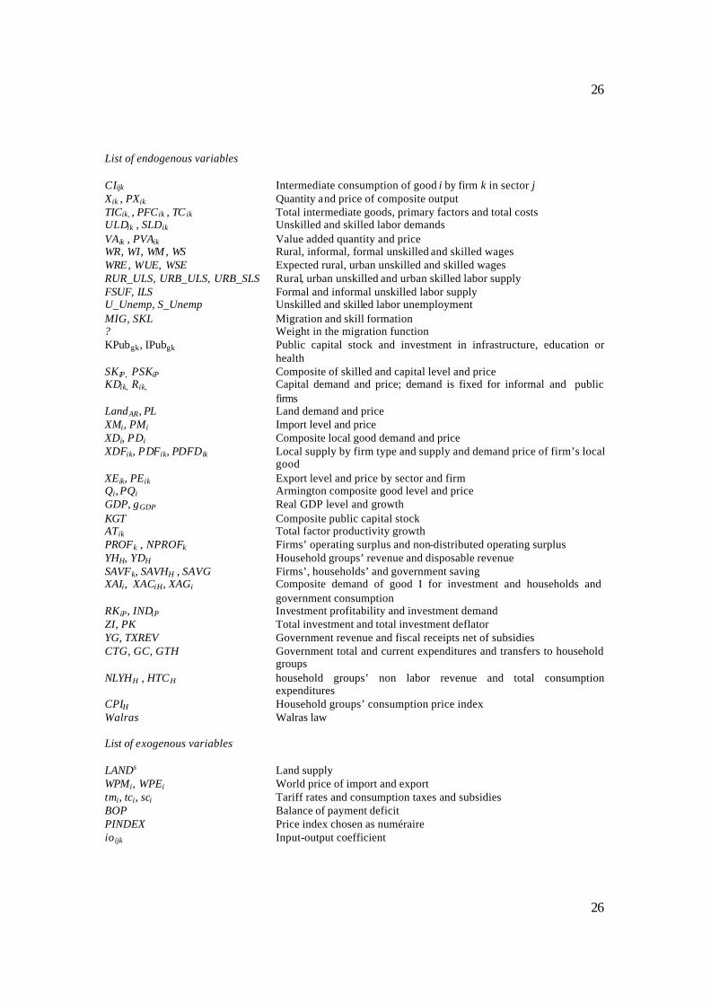
List of endogenous variables CIijk Intermediate consumption of good i by firm k in sector j Xik , PXik Quantity and price of composite output TICik, , PFC ik , TC ik Total intermediate goods, primary factors and total costs ULDik , SLDik Unskilled and skilled labor demands VAik , PVAik Value added quantity and price WR, WI, WM , WS Rural, informal, formal unskilled and skilled wages WRE , WUE, WSE Expected rural, urban unskilled and skilled wages RUR_ULS, URB_ULS, URB_SLS Rural, urban unskilled and urban skilled labor supply FSUF, ILS Formal and informal unskilled labor supply U_Unemp, S_Unemp Unskilled and skilled labor unemployment MIG, SKL Migration and skill formation ? Weight in the migration function KPubgk, IPubgk Public capital stock and investment in infrastructure, education or
health SKiP, PSKiP Composite of skilled and capital level and price KDik, Rik, Capital demand and price; demand is fixed for informal and public
firms LandAR, PL Land demand and price XMi, PMi Import level and price XDi, PDi Composite local good demand and price XDFik, PDFik, PDFDik Local supply by firm type and supply and demand price of firm’s local
good XEik, PEik Export level and price by sector and firm Qi, PQi Armington composite good level and price GDP, gGDP Real GDP level and growth KGT Composite public capital stock ATik Total factor productivity growth PROFk , NPROFk Firms’ operating surplus and non-distributed operating surplus YHH, YDH Household groups’ revenue and disposable revenue SAVFk, SAVHH , SAVG Firms’, households’ and government saving XAIi, XACiH, XAGi Composite demand of good I for investment and households and
government consumption RKiP, INDiP Investment profitability and investment demand ZI, PK Total investment and total investment deflator YG, TXREV Government revenue and fiscal receipts net of subsidies CTG, GC, GTH Government total and current expenditures and transfers to household
groups NLYHH , HTCH household groups’ non labor revenue and total consumption
expenditures CPIH Household groups’ consumption price index Walras Walras law List of exogenous variables LANDs Land supply WPMi, WPEi World price of import and export tmi, tci, sci Tariff rates and consumption taxes and subsidies BOP Balance of payment deficit PINDEX Price index chosen as numéraire ioijk Input-output coefficient