Trade Reforms, Income Distribution and Welfare: The ... · PDF fileTrade Reforms, Income...

RESEARCH PAPER

SERIES No. 2002-03

Caesar B. Cororaton

Trade Reforms, Income Distribution

and Welfare: The Philippine Case

PHILIPPINE INSTITUTE FOR DEVELOPMENT STUDIESSurian sa mga Pag-aaral Pangkaunlaran ng Pilipinas

This study was funded by the International Development Research Centre(IDRC) of Canada. It benefited greatly from the series of discussions withthe CREFA (Centre de récherche en economique et finance appliqués)group of Laval University in Quebec City, Canada.

The author, Dr. Caesar B. Cororaton, is a senior research fellow of thePhilippine Institute for Development Studies. His areas of expertise includeapplied general equilibrium modeling, total factor productivity estimation,and trade and poverty analysis.

Trade Reforms, Income Distributionand Welfare: The Philippine Case

Caesar B. Cororaton

RESEARCH PAPER SERIES No. 2002-03

PHILIPPINE INSTITUTE FOR DEVELOPMENT STUDIESSurian sa mga Pag-aaral Pangkaunlaran ng Pilipinas

Copyright 2003Philippine Institute for Development Studies

Printed in the Philippines. All rights reserved.

The views expressed in this paper are those of the authors and do notnecessarily reflect the views of any individual or organization. Pleasedo not quote without permission from the author nor PIDS.

Please address all inquiries to

Philippine Institute for Development StudiesNEDA sa Makati Building, 106 Amorsolo StreetLegaspi Village, 1229 Makati City, PhilippinesTel: (63-2) 893-5707 / 892-4059Fax: (63-2) 893-9589 / 816-1091E-mail: [email protected]: http://www.pids.gov.ph

ISBN 971-564-058-3RPO3-O3-SOO

Table of'Contents

VllAbstract

I. The Philippine Economy: Growth Performanceand Basic Structure

1

II. Trade Reforms 6

III. 15Income Sources, Distribution and Poverty

IV. Model Description 20

v. Simulation Results 23

VI. Conclusion 41

Appendix 42

ill

List of Tables, Figure and Appendix

Table Page

123456a6b6c7a7b

23358

1010111212

89101112131415

1316171825262627

16 30

17 31

18 33

19 35

20 35

21 36

22 38

3923

The Philippine EconomyProduction StructureEmployment StructureProduction and Factors (1990 Social Accounting Matrix)Trade ProtectionExports (million US dollars)Imports (million US dollars)Import and Export Share (1990 Social Accounting Matrix)National Government BalancesNational Government Balances: Percentof Gross National ProductAverage Tax Rates (1990 Calibrated SAM values)Sources of Income in 1990Household Consumption (1990 Socia! Accounting Matrix)Distribution and PovertyBase Values of Some Relevant VariablesBase Values of Household Income SharesBase Values of Some Relevant Micro VariablesTrade Effectts (scenario: zero tariff and'compensantory income taxes)Production Effects (scenario: zero tariffand compensatory income taxes)Consumption Effects (scenario: zero tariffand compensatory income taxes)Effects on Sources of Income (scenario:zero tariff and compensatory income taxes)Income and Welfare Effects (scenario:zero tariff and compensatory income taxes)Macroeconomic Effects (scenario:zero tariff and compensatory income taxes)Trade Effects (scenario: actual tariff andcompensatory income taxes)Production Effects (scenario: actual tariff andcompensatory income taxes)Consumption Efrects (scenario: actual tariffand compensatory income taxes)Effects on Sources of Income (scenario: actualtariff and compensatory income taxes)

24 40

25 Income and Welfare Effects (scenario: actualtariff and compensatory income taxes)Macroeconomic Effects (scenario: actualtariff and compensatory income taxes)

40

26 40

Figure

1 Basic Price Relationship in PCGEMX 21

Appendix

1 Equations and Variables: PCGEM Model 42

lJ

Abstract

In the past one and a half decades, the Philippinegovernment pursued major economic policy reforms. One ofthe key focused areas is the trade sector. Policy reformsincluded tariff reduction, simplification of tariff structure, andtariffication of quantitative restrictions. While some of thereforms were pursued unilaterally, others were done undervarious multilateral agreements such as the World TradeOrganization (WTO), and regional agreements under theAssociation of Southeast Asian Nations (ASEAN) such as theASEAN Free Trade Area (AFT A). This paper aims to analyzethe effects of the trade reforms, particularly tariff policies, onincome distribution and welfare. The paper employs acomputable general equilibrium (CGE) model calibrated toPhilippine data in the analysis.

vii

I

The pIiilippine Economy:Growth Perfonnance and Basic Structure

The last 35 years sa a "roller coaster" Philippine economicgrowth performance. rowth was highest during the 1973-1982 period, averagin 5.5 percent per year (Table 1). Whileconsidered by many a the peak period of the Marcos regime,such excellent perfor ance was not sustained, however, asdissatisfaction among .pinos on the military regime mountedand eventually led to a olitical uprising in the following period,1983-1985. The politic crisis triggered an economic crisis thatresulted in an econo ic collapse. During that period, theeconomy contracted y -4.1 percent per year. The Marcosadministration was f y forced out in the early part of 1986,which gave way to th Aquino government.

In the following pe iod, 1986-1990, the euphoria under thenew government bro1J ht about economic recovery. Growthaveraged 4.5 percent p r year during that period. Toward theend of the Aquino ad .istration, however, the political tug-of-war led to a series of 'litary coup attempts. Although theseattempts failed, they created political uncertainties andinstability. These, toge er with the series of natural calamitiesand the energy crisis, rought the economy to a halt in 1991-1993. During that per' d, the economy contracted again by-0.1 percent per year.

The new governm nt after Aquino was able to revive theeconomy. Under the mos leadership, growth averaged 4.9percent per year from 994 to 1997. But this improvement wasshort-lived. The comb' ed effects of the Asian financial crisisthat began in 1997, t e El Nino in late 1997 that prevailedunti11998 and severel affected agricultural production, andthe political scandals in the Estrada administration took a

1

Trade Reforms, Income Distribution and Welfare

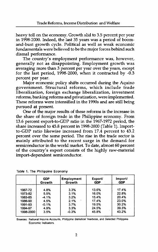
heavy toll on the economy. Growth slid to 3.5 percent per yearin 1998-2000. Indeed, the last 35 years was a period of boom-and-bust growth cycle. Political as well as weak economicfundamentals were believed to be the major forces behind suchdismal performance.

The country's employment performance was, however,generally not as disappointing. Employment growth wasaveraging more than 3 percent per year over the years, exceptfor the last period, 1998-2000, when it contracted by -0.3percent per year.

Major economic policy shifts occurred during the Aquinogovernment. Structural reforms, which include tradeliberalization, foreign exchange liberalization, investmentreforms, banking reforms and privatization, were implemented.These reforms were intensified in the 1990s and are still beingpursued at present.

One of the major results of these reforms is the increase inthe share of foreign trade in the Philippine economy. From13.6 percent export-to-GDP ratio in the 1967-1972 period, theshare increased to 45.8 percent in 1998-2000 (Table 1). Import-to-GDP ratio likewise increased from 17.4 percent to 43.2percent over the same period. The rise in the trade sector ismainly attributed to the recent surge in the demand forsemiconductor in the world market. To date, almost 60 percentof the country's export consists of the highly raw-materialimport-dependent semiconductor.

Table 1. The Philippine Economy

GDPGrowth

EmploymentGrowth

Export!GDP

Import!GDP

13161517192445

17.4%22.8%20.4%23.0%30.2%39.3%43.2%

1967-721973-821983-851986-901991-931994-971998-2000

4.5.

-4.4.-0.4.3.

3.:3.3.2.3.3.

-0.

Sources: National Income Accounts, Philippine Statistical Yearbook, and Selected PhilippineEconomic Indicators.

2

6%0%4%4%5%5%8%

8%5%1%5%

1%9%5%

~%1%

~%1%r%

~%~%

Growth Performance and Basic Structure

In spite of the reforms and the dramatic rise in foreign trade,there are obvious signs of structural weaknesses in the localeconomy. These are evident in the stagnating shares of theindustry and manufacturing sectors over the past 35 years(Table 2). The share of industry picked up from 31.7 percentin 1967-1972 to 37.4 percent in 1983-1985. Then it began todrop and continued to do so through 1998-2000 leaving a 30.9percent share. A similar dismal record for the manufacturingsector is observed over the same period. The agriculture andservice sectors, however, exhibited opposing trends: while theshare of agriculture steadily dropped from 1967-1972 through1998-2000, the share of the service sector continued to rise.

The disappointing and stagnating share of the industry andmanufacturing sectors is also observed in the structure ofemployment. Employment share in industry is about 15percent, while its share in manufacturing is 10 percent (Table

Table 2. Production Structure

Sources: National Income Accounts, Philippine Statistical Yearbook.

Table 3. Employment Structure

Sources: Philippine Statistical Yearbook

3


3). These shares have practically stagnated as compared to therising employment share in the service sector.

The contrasting performance of the foreign trade andindustrial sectors, in general, and the manufacturing subs ector,in particular, in terms of output and employment generationamid the policy reforms, indicate the absence of any trickledown effects. Considering that these policy reforms have beenpursued for quite sometime, the lack of concrete trickle downeffects would strongly imply a high degree of duality existingbetween the local and foreign sectors. .

Table 4 shows a detailed sti"ucture of production of theeconomy based on the official 1990 Social Accounting Matrix(SAM). The agriculture and service sectors have high valueadded content as compared to the industry sector. Electricalequipment manufacturing, whose major operation is theproduction of semiconductor, has a value added ratio of 15

\percent.

About 78 percent of the overall value added is payment tocapital. Payment to labor accounts for only 12.4 percent, whilethe rest is payment to variable capital, which is officially calledmixed income. Across sectors, however, the composition varieswidely. It is important to note especially in income distributionanalysis that payment to variable capital in agriculture capturesmore than 30 percent of the value added. In fact, in palay andcorn production, payment to variable capital is almost 83percent. In livestock and poultry, it is 56.2 percent, while infruits and vegetable it is 45.8 percent. In conti"ast, in industi"y,the share of payment to capital is below 10 percent, except forgarment and leather (13.7 percent) and fish manufacturing(10.2 percent). In the service sector, the only subsector withhuge payment to variable capital is private health.

4

-)('C"IV~ac~;1C

/)..0UtVu."0CtVc.2U~"00..Q

.

~Q)

:is~,

~Go

~() "C""C"C<~ii'> "C.,"C~.,.2 ~

~

L~~

~~

~~

~~

~~

q~~

~~

~~

~~

~q~

~qq~

~q~

=

~

~

~

~ ~

N

~

~

~

~

~

0 N ~

0 N

~

~

~

., ~

0

~

~

0 0

~

N 0

~..0-f

to.!

~U

) :g

~ ~

-to,~

>

~ ~

~ ~

~~

~~

~~

~~ ~

R~

~

~~

~~

~~

~~

~

~~

~

Mm

-m~

-O

0- -00-0-000

000

--U

~

..~II.

.,~

:0

0 s

j ~-~0.0..-'~!:;.U

)

~Q~~~~U)

:D"

e:-O

)~~ ~I~

~

~ ~

~ ~

:'.1jl~

a ~ ~

E ~ ~

~~~

~~

!--;:-;- ~

:!!s~~

m:~

~.g°M

NN

-NO

j ~~

8~~

~~

~~

~~

~~

~~

~~

~~

~q~

~~

~~

~~

$~~

~~

~~

~~

~~

SO

~N

ON

~~

~N

~~

MO

M~

O~

~O

MM

~~

OO

om~

2moooooM

M8

-~Co

..U

onQJ

~~

~

~

wE

8, ~

X

"'

~I

OQ

J~a:

a ~

<.;;:;; ~

~

5,

~

Iffiffi~

'gg'o( u

>-$JO

"-~on~

"-(')QJ~

~Q

J1O

2o>--b~

Q.LLU

::JLLQLLo(

"!'-:"1"""1"!II!.1"1~"'W

"!CO

~O

CO

CO

"'~C

O"""I'-O

~I'-~

!88!~R

5!~~

R~

gj~~

~~

'§:Ij~~

~ijjw

'~~

!g:lj~~

;:

I::J

~ s ~

~ ~

~I

~~

~~

~m

~~

~v~

~~

M~

~m

~vvo~

~~

ov~~

~2~

~~

~~

~~

~~

~~

~~

~~

~~

~~

N~

~~

~~

~

I~ ~ ~

~;: ~

~

"1O!q..,'":~

Q1

"'Q~

o)"'o)N

Grow

th Perform

ance and Basic Structure

~~

~~

~~

~~

~~

~Q

~99~

~~

~~

~~

~

~

~

~

0

~

~

~

N

~

~

., o.

., .,

N

~

., ~

N

~~

~~

~~

~q~

~~

~~

~~

~~

~~

~~

~

~

"ON

0

~

.0 ~

0

0 ~

~

0

0 0

0 0

m

N

~~

~~

~~

~~

~Q

~~

~~

~~

Q~

~~

~~

~~

N~

~N

N~

O~

W~

OW

W~

O~

NN

~~

~

~

~

~~

~~

q~~

~~

~~

~~

~~

~q~

~~

~~

~~

~~

~~

~~

~~

~~

~$~

~~

~~

~~

~m

mm

~~

~i~

~2~

~~

~

S~

S!~

l8l11~~

8!~~

Gi~

~!!!8!~

~P

-IP-I~

¥!!R~

~~

3:~~

~N

OO

~O

~N

O~

OO

~O

OO

~O

O~

~::!"'N

O«J~

~~

'"c:

~"'~§ c:

2~~

~g'

'" c:~

~

c: ~

'" c:

"'.0: -

" ~

c: §

~

u '"

'" """

§U

g'~g'"O

§,,,Ug'c~

g' ~

~

§ §~

",~§£c:e;gS

~§~

~§

-g E

'=

"5.cC:U

m~

Q."c:c:U

c.£U

'" 56

6 ~

~~

~uu~

~"'..J~

8.ffi~~

~50~

on

~~

£~

~zs

8 ~~

~05~

~05~

"'~

~E

-e,y;05~

6~~

cn:sm

~~

Q

~U

)"C

:c:Q)om

on.!2Q.-

!9",-t",tj -_"O

:r:"OQ

)C!)Q

)W"'~

U).!2~

~

u. C-~

~05 ~

ffi w~

B

8.~ 2:01;;

~'i\:

Q)w

:r:~(/)~

~c:~

"O~

~"~

.!! ~

Eol;:-C

:on~u;

~C

:--!,!!,!Q)~

'"

s8~m

~~

~~

",8~J.~

6~~

~~

6~Q

~~

~:g:g~

~ffib

~~

~~

~~

O~

~~

~U

Q.z~

w~

ouw~

cQ.Q

.Q.Q

.C!)O

U)~

5

'f

~~

"!IX!,"",!",IX

!,",,",

~~

~~

~/'-~

~~

~

g

FIF

,,!q,,!~~

,,!,,!~

"'~O

NO

"'~"" '"

r'":"1"1"""""

"""~;:~

:SR

'",

~I

C'f~

q q

q "1

jQIQ"~

ooo~",g ~

al~

"tIC

!

~~

~I~

'"'II'!!!!~

$I

~

~~

q§

mu<n

~><

."1U~0).5'E~°8<

{ Q

I

:§ E

u 0

°-g u

<n "C

:s .5

o"C.9-"C

O)C

O~

QI

~ Q

lO.!!

..-=-;n

EQ

lCO

...

~>

8E~

.~o

o~O

~<

n»<.

II

Trade Reforms

A number of trade reform programs were implementedbefore the 1990s, but the major one was started in the early1980s. The program had three major components: the 1981-1985 Tariff Reform Program (TRP), the Import LiberalizationProgram (ILP), and the complimentary realignment of theindirect taxes. In the TRP, there was a narrowing of the tariffrate structure from 100-0 percent to 50-10 percent. Duringthe period 1983-1985, sales taxes on imports and locallyproduced goods were equalized. Also, the markup applied onthe value of imports (for sales tax valuation) was reduced andeventually eliminated.

However, because of the balance-of-payments crisis duringthe mid-1980s, the import liberalization program wassuspended. Some of the items that were deregulated earlierwere re-regulated.

The trade reform program of the early 1980s was resumedwhen the Aquino administration took over in 1986. Thisresulted in the reduction of the number of regulated items from1,802 in 1985 to 609 in 1988. Furthermore, export taxes on allproducts except logs were abolished.

In 1991, the government launched a major-trade reformprogram with the issuance of Executive Order (EO) 470 calledthe TRP-II, an extension of the previous program. Tariff rateswere realigned over a five-year period. The realignmentinvolved the narrowing of the tariff rates through a series ofreduction in the number of commodity lines with high tariffs,and an increase in the number of commodity lines with lowtariffs. In particular, the program was aimed at clustering thecommodities with tariffs within the 10-30 range by 1995.Despite the programmed narrowing of the tariff rates, about

6

Trade Reforms

10 percent of the total number of commodity lines were stillsubjected to 0-5 percent tariff and 50 percent tariff rates bythe end of the program in 1995.

"Tariffication" of quantitative restrictions (QRs), that is,converting them into tariff equivalent, started in 1992 withthe implementation of EO 8. There were 153 commoditieswhose QRs were converted into tariff equivalent rates. Also,under the same EO, tariff rates on 48 commodities were furtherrealigned. EO 8 raised the tariff rates applicable to the relevantcommodities by 100 percent of their pre-EO 8 levels. In effect,the tariff rates imposed were higher than the tariff equivalentrates in a number of cases, especially during the initial years ofthe conversion. However, EO 8 has a built-in program for afive-year phase-down of the "tariffied" rates.

Under the import liberalization program, deregulationcontinued on 286 items. At the end of 1992, only 164commodities were covered under the QRs. However, theimplementation of Memorandum Order (MO) 95 in 1993reversed the deregulation process. In fact, QRs were reimposedon 93 items, bringing up the number of regulated items underthe QR to 257. This re-regulation came largely as a result ofthe Magna Carta for Small Farmers in 1991.

Major reforms were implemented under TRP-III. Theprogram was embodied in the following EOs: (i) EO 189implemented in January 1, 1994, which provided reduced tariffrates on capital equipment and machinery; (ii) EO 204implemented on September 30, 1994, which mandated tariffreduction in textiles, garments, and chemical inputs; (iii) EO264 implemented on July 22, 1995, which reduced tariffs on4,142 harmonized lines in the manufacturing sector; and (iv)EO 288 implemented on January 1,1996, which reduced t~riffson "nonsensitive" components of the agriculture sector.Restructuring of tariff under these EOs means reducing thenumber of tariff tiers and the maximum tariff rates. Inparticular, the program was aimea at establishing a four-tiertariff schedule, namely: 3 percent for raw materials and capitalequipment that are not available locally; 10 percent for rawmaterials and capital equipment that are available from localsources; 20 percent for intermediate goods; and 30 percent forfinished goods.

.,

Trade

Reforms

protection. Under the World Trade Organization (WTO)agreement, quantitative restriction on rice is still allowed.

Increasing implicit tariff rates were seen in some sectorsduring the early 1990s. This was largely due to the effects ofthe "tariffication" of quantitative restrictions. However, fromthe mid-1990s to the turn of the century, all of the sectorsexhibited a declining trend. Food manufacturing had thehighest implicit tariff, while mining had the lowest.

Manasan and Querubin (1997)1 analyzed the impact ofthe different trade and tariff reform programs in the 1990s onthe structure of tariff. In particular, they computed the implicittariff rates and effective rates of protection (EPRs) for 169commodities based on domestic and border prices. They foundthat as a result of the series of reforms, significant achievementswere attained in the area of tariff simplification. Over time,the program restructured the tariff system from a 5-level to a3-level rate schedule. Moreover, most of the commoditiescluster around the 3-20 percent range.

Furthermore, based on the results, they observed gains inthe form of reduction in the average nominal and implicit tariffrates, as well as in the EPRs over the period 1990-2000. Overall,the average nominal tariff rate decreased from 33.3 percent in1990 to 19.5 percent in 2000. Likewise, the average implicitrate based on price comparison declined from 28.6 percent in1990 to 16.8 percent in 2000. In addition, the overall EPR basedon price comparison dropped from 29.4 percent in 1990 to18.0 in 2000.

It was also observed that the decline in the EPRs ispronounced in the manufacturing group than in the primarygroup, particularly in the agriculture subgroup. This implies aswitchover in relative protection in the agriculture andmanufacturing sectors. Relative protection is observed toincrease from 1995 to~OOO, in sharp contrast to the previousdecades when the agriculture sector was penalized heavilyrelative to the manufacturing sector. During the period 1990-1994, the manufacturing group enjoyed relatively higherprotection than the agriculture sector. There was a majorswitch during the period 1995-2000 in favor of agriculture.

1 Manasan, R.G. and R.G. Querubin. 1997. Assessment of Tariff Reform in the 1990s.

PIDS Discussion Paper Series No. 97-10.

9


What are the effects of these trade reforms on the structureof the foreign trade sector? Table 6a shows the structure ofexports and Table 6b shows the structure of imports. Table 6cpresents the structure of both in 1990 according to the SocialAccounting Matrix (SAM) industry breakdown. Manufacturedexports increased its share to the total from almost 70 percentin 1990 to 91.2 percent in 2000. The increase is mainly due tothe surge in exports of electrical equipment, mostlysemiconductor, which captures almost 60 percent of thecountry's export. On the other hand, the share of importation

Table 6a. Exports (million US dollars)

Share (%)1990 I 1995 2000j 1990119951 20001

503 989 595133 74 57326 458 528431 575 486

94 38, 44723 893 650I

155 171 4365,707 Iv,86833,9891,964 7,413 22,1781,776 2,570 2,563

93 208 2491 ;874 3,677 1 8,999

114 381 502

Coconut Products 1.6Sugar and Products 0.2Fruits and Vegetables 1.4Other Agro-based Products 1.3Forest Products 0.1Mineral Products 1.7 I

Petroleum Products 1.2Manufactures 91.2Electrical and Electrical Equipmem 59.5Garments 6.9Textile Yarns/Fabrics 0.7Others 24.1

orts ~-1QQ,9--

unt BalanceSource: Selected Philippine Economic Indicators. ang 0 entra rig Ilplnas.

Table 6b. Imports (million US dollars)

Capital GoodsRaw Materials and IntermediateGoods

Unprocessed Raw MaterialsSemi-Processed Raw MaterialsChemicalsTextile Yarn/FabricIron and SteelMaterials for Eletrical EquipmentOthersMineral Fuels abd LubricantsConsumer Goods

I OthersI Total Imports

Source: Selected Philippine Economic Indicators, Bangko Sentral ng Pilipinas.

10

Trade Reforms

Table 6c. Import and Export Shares (1990 Social Acounting Matrix)

Shares (%)

Imports0.420.430.050.250.301.850.23

3.53 I

8.91]0.92

0.060.210.050.933.264.043.460.181.317.552.181.598.169.469.844.010.050.00

66.19

2.580.000.090.000.000.00

27.6130.28

100.00

358.58

Exports

0.011.660.140.212.160.91

0.165.25

2.21

0.061.050.010.710.402.412.47

12.751.881.511.851.881.022.72

11.751.169.120.070.64

55.67

1.01

0.000.150.000.000.00

37.9239.08

100.00

297.98

-51.71

Palay and CornFruits and VegetablesCoconut & SugarLivestock & PoultryFishingOther Agriculture

ForestryAGRICULTURE

MiningRice & Corn MillingMilled SugarMeat ManufacturingFish ManufacturingBeverage & TobaccoOther Food ManufacturingTextile manufacturingGarments & LeatherWood ManufacturingPaper & Paper ProductsChemical ManufcturingPetroleum RefiningNon-metal manufacturingMetal ManufacturingElectrical Equipment ManufacturingTransport & Other Machinery ManufacturingOther ManufacturingConstructionElectricity. Gas and Water

INDUSTRY

Financial SectorPrivate EducationPrivate HealthPublic EducationPublic HealthGeneral GovernmentOther Services

..SERVICES

I

TOTAL

Total Value (Pb)Current Account Balance (P billion)

Source: 1990 Social Accounting Matrix, National Satistical Coordination Board.

11


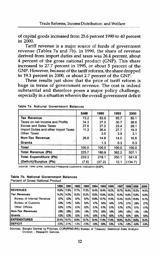
of capital goods increased from 25.6 percent 1990 to 40 percentin 2000.

Tariff revenue is a major source of funds of governmentrevenue (Tables 7a and 7b). In 1990, the share of revenuederived from import duties and taxes was 26.4 percent, about4 percent of the gross national product (GNP). This shareincreased to 27.7 percent in 1995, or about 5 percent of theGNP. However, because of the tariff reforms, the share droppedto 19.3 percent in 2000, or about 2.7 percent of the GNP.

These results just show that the price of tariff reform ishuge in terms of government revenue. The cost is indeedsubstantial and therefore poses a major policy challenge,especially in a situation wherein the overall government deficit

Table 7a. National Government Balances

Source: 1990 SAM, Selected Philippine Economic Indicators (BSP).

Sources: Bangko Sentral ng Pilipinas; COR(FPAD-RS) Bureau of Treasury: Statistical Data AnalysisDivision -Research Service.

12


is not only huge but is also ballooning. From surpluses in themiddle of the 1990s, government balances flipped to deficitstarting 1998, and deteriorated since then to -3.9 percent ofGNP in 2000. The culprit was the tax revenue generationbecause while the expenditure ratio was within the 18 percentratio to GNP, the tax ratio dropped from 16.3 percent in 1996to 12.9 percent in 2000. This shows that the viability of anytariff reform program depends significantly on how revenuegeneration from local taxes can improve to offset whatevertariff revenue losses the government may incur.

14

III

Income Sources, Distribption

and Poverty I

Table 9 shows the sources of income of households, ascaptured in the 1990 SAM. There are im ortant differencesacross decile categories of household that have to behighlighted. Of its total income; the first ecile sources 12.7percent from agriculture labor income an the second decilesources 13.1 percent. The share declines a one moves up tothe higher deciles. For the tenth decile, agric lture labor incomeis only 0.7 percent of its total income.

The opposite trend is observed in no agriculture laborincome. The first decile sources 6.7 percent of its income fromthis source, while the ninth and tenth d ciles source 39.9percent and 32.8 percent, respectively. ixed income fromagriculture is a major source of income f the first decile,capturing 47.1 percent of the total. It dec ases significantlyas one moves up to the higher decile grou s. The tenth decilesources only 6.3 percent from agricultu e mixed income.However, for mixed income in nonagricultu e, it is the opposite.The tenth decile sources 32.8 percent of it income from thissource, while the first decile sources only 0.2 percent.

Table 10 presents the structure of house old consumption.On the whole, household consumptio is 13.65 percentagriculture-based, while 48.94 percent is industry-based.Household consumption is 37.41 percent s rvice sector.:.based.

Interestingly, poverty incidence droppe from 44.2 percentin 1985 to 35.5 percent in 1994 to 31.8 per ent in 1997 (Table11). However, the latest poverty informati n in 2000 indicatesthat this declining trend is reversing, with th incidence inchingup to 34.2 percent.

15

Trade R

eforms, Incom

e Distribution

and Welfare

0aIaI...CQ

)

E0(Jc-0IIIQ)

(J...~0(/)

aIQ)

:c~

16

.;:§InI:

~-c:0)EE0)>0C

)

"CI:~.,-~5u0)In

-c:0)EE0)>0C

)

E.g0)

.E"E

8~

I:

0.-m

-In

I: I:

.2.9roroI:

~.-0"E

o.0

~

08U

O)

"(Om

.2 .~

~5.

ro"C-I:cn~"(O

"CI:

0)0-:O

J~~

0

ze-.0

x U

.1: I:

ro .2

~

J

C)E

I: 0

:OJ.;I:J

In0

0)U

E

U

0~

U

-I:~ .-'u

"C0

I:cn

0)"C

0.-0>

.~O

>"C

'-:0)"C0)

J

~-J U

oEcn-

~'~"iU~C

IC;C~0C

o)C

o)«"'iij'u0(/)

00)0)

~C0c.E~U)

c0U"C"0.r.U)

~0~0...G>

:c~

-00":

c, .",-:~~

~,,!

,;:~ ;.c. "'~

;::~~

~

~"':".~

'" ~

~,,!,-:~

~

'":~~

~

"!~~

ON

_~"'~

~;

~.~

~N

~O

N~

~~

O~

ON

~~

"'NO

.~~

~O

OO

~G

~ ..-~

..."'~

N~

N

~

~

~

~

... ~

~

.GG

~..

I') N

N'"...~

;;>.~-~

OO

"""~"'~

~~

-~~

~N

~.N

~N

-~N

~"'O

.~~

~~

.ON

~C

_o~~

~m

"'.C~

"'Om

~N

.~~

O.~

N~

~"'.O

N~

~~

~-O

OO

-.C

~O

~O

~~

oo~O

m~

m~

MO

ON

~O

~O

~O

~O

~O

~.O

NN

OO

ON

~O

.-.~I')C

~

C.N

~"'N

~.~

OO

~"'N

O~

"'~

O-~

N."'.N

NN

.~~

O~

.C

~O

~-~

O~

.~N

O~

-~~

"'~"'.~

~N

~..~

-~N

GN

~~

OO

O~

CC

~O

~Q

~~

OO

~O

~O

~~

N~

ON

~O

~O

~O

NO

~O

~~

~N

NO

OO

~~

O~

.. .~

.~

~~

.~~

~.~

~

~...~

...~~

m-"'~

~O

N~

N"'~

.~.~

~~

.ON

~C

~O

~

~

. 0 ~

~ N

N

~ ~

~.

~ N

. ~

~.

ON

~

~ ~

~ ~

OO

O

~ ~

C~

6~O

~~

oo~O

m~

m~

MO

ON

-O~

O~

O~

O~

O~

.ON

NO

OO

N.O

~

-.~I')~

G~

.~N

-~~

~~

.oo.m~

~.~

.-~~

~~

"'N~

N.m

m"'~

.Om

NC

~O

~-~

o m

-N~

~"'~

~~

.~N

NN

~~

ON

~G

"'~-O

OO

~N

C

~O

~O

~~

oo~O

m~

O~

MO

ON

OO

~O

~O

~O

~O

~m

ON

NO

6oo.o"

--.~I')~

"'~O

"'~~

N"'~

~O

~~

N~

N~

~"'-~

~O

~"'I')~

~~

~.~

.~.O

~N

C

~O

O-~

N~

.~:-.-~

"""N~

~G

.NN

ON

.l')mN

NG

"'OO

OO

O~

GC

~O

~O

~~

OO

~O

O~

O~

M~

ON

OO

~O

~O

~O

OO

~O

ON

NO

OO

m~

O

.; ---~

N

I')~

G~

~'"

NO

."'~ci

~ -0

O"'~

-~-N

OO

~~

~~

o. -O

NO

~..~

O

~~

C

~O

O-~

.~.

-"'-O"'~

~~

~~

~N

NO

N~

~O

N~

~"'O

OO

OO

~~

C

~O

~O

~~

OO

~O

O~

~~

M~

ON

OO

~O

~O

~O

OO

~~

O~

~O

OO

~~

O.;

---~

N~

~

~~

N~

~N

~"'~

~

O~

.~.~

~~

NN

~~

mm

O~

~O

~.~

OO

CC

~O

~-~

~~

.~--N

.~~

~~

~"'~

-NO

NN

N~

-~N

~~

"'OO

Om

NC

~O

~O

~~

OO

~O

~~

~~

M~

ON

OO

~O

OO

~O

OO

~N

O~

~O

OO

~N

O;;

---~

N~

~

.~~

~N

.O~

~."'~

~~

~

~-~

~N

~~

"'~.-~

~~

~~

O~

"'C

~o.-o...m

._-~N

~~

~O

~~

"'~~

N~

N-N

~-~

"'~"""O

OO

N.C

~O

~O

N~

OO

~O

~~

~~

MN

ON

OO

-OO

O~

OO

O~

NO

~~

OO

O~

~O

.~

--~

N~

C~

M~

~O

Om

~."'~

~~

~~

~~

..~~

-N~

..m~

NO

"'~.~

O--C

~o~

-o...m

N"'~

"'O~

"""~O

Nm

NN

N~

~~

G~

~~

OO

ON

NC

~O

~O

N~

OO

~O

~~

~~

MN

ON

OO

~O

OO

~O

OO

~N

O~

~O

OO

~~

O~

---~

N

~~

N~

"'~N

-~N

~.O

~.O

m~

O~

Nm

m"'~

~-N

~~

~C

N~

.~~

O~

GC

~o~

--~m

~~

--~.O

~~

~~

~N

mN

"'-ON

~

..ooom.c

~O

~O

N~

OO

~O

N~

NN

MN

ON

OO

OO

OO

~O

OO

~~

O~

~ooo~

mo

~

~

NN

C~

~.~

~o~

~m

"'ON

~~

~.~

o_m~

N~

"'__I')~O

~~

C

~

'": ~

~

~

~~

"!~

~

~~

~

'-: ~

~

~

~

~

~~E

~

'": ~

~~

~~

... ~

~

ON

-NN

~N

ON

QO

OO

OO

-OO

O~

~O

~-O

OO

~G

C-,.

-~

NN

C'-

r;

~

~-~

~~

G"'O

~o)~

'" ~

OO

N~

No)'"

~O

"':ON

cDO

O

Income S

ources, Distribution and P

overty

17

,

.~~vcoO

I~cc

." co

,,~V

>-

~~""

~01

-CC

.,

C

~,._-

.-"' "

C

CO

.c -

~

VO

l." ~

u

.."'

-01 "C

" C

O

s:.,

OU

C~

OI"O

." -O

I-~O

I C

:0 ~

01

!2'OIU

U~

."".=O

"OIgc~

C

"5!

.,C

O -C

~

C

"".c~~

-C_.-

~."

~

CE

-iU3.,

=

."."coc-.."a.J:!.-="~

E",,

CO

~

O

CC

., 0

~

-" "

.c u

-,,- C

-C

o.c -0.-

0 C

Og'g'a.

~

~

vv~~

~~

g~~

~~

g.s6g ~

v";~

.c~~

u>tI>

0/5 ~

E

iU-5~

0/5"O~

0/5a~~

a: ~

~0/5ag~

~,~

g~~

~co

~.~

1/1~

.- -"

0C

O -

a.E

-C

--~

v'"O

--,. ~

"O"O

~~

~

o~

,cc"E

"'co -IV

CO--C

O-

~W

~"O

"v..WC

C

01 U

"CO

-0

-~

CO

-C

O~

u-

-~W

~

-C

O CO

-:; g 0I-t

~

tI> ~ ~

O

ILL C

~ 0/5 u ~

., ~

U 0 ~

".U

:n ~

.,., ~

iU tI>

~C

-C

OJ

010/5 ~

~

~

., ., "0

~ .E

-E

." C

o ~ ;; ."

u --u u

~

~ >

.J~

:4. 8

~:2

~.,

.=.,

~...c

~ .,:;;

§ 0 ~

., e

c:§ v

~

., ~

v ~

~

~

~

:s:s ~

., ~

~

iU20.~

.~;o

.=.!!=

".~";)(IV

Oco.ca;o"~

~;o~

Q.=

.".""".,;wo

a.LLU.JLLO

LL ~

a:~~

LLmO

~~

s:a.ua.z~W

~O

UW

~LLa.a.a.a.~

OI/l~

"E~0mc.Qmc'E00u~§mci5

"iijcQmzx'cm~OJ

.=C~8u~"iij'u0cn0~O

J~~0cn

I


Table 11. Distribution and Poverty

Source: NatiQnal Statistical Coordination Board and National Statistics OfficeNote: NCR is National Capital Region, and CAR is Cordillera Autonomous Region

There are huge discrepancies in poverty incidence acrossregions, with the National Capital Region (NCR) where MetroManila is located having the lowest poverty incidence. Therewas a significant drop in poverty incidence in the NCR from23.0 percent in 1985 to 8.0 percent in 1994 and further downto 6.4 percent in 1997. The trend reversed in 2000 as povertyincreased to 9.7 percent.

Although poverty incidence in areas outside the NCR alsodropped over the same period, such reduction was~onsiderably less th~ in the ~CR. In 1997, poverty ~ldencem these areas was still very hIgh at 35.9 percent and it furtherincreased to 38.3 percent in 2000. In poorer regions like theCordillera Administrative Region (CAR), poverty incidencein 1997 was still above 40 percent, although it slightly droppedin 2000. Based on these indicators, two points are worth noting:(1) there is an apparent substantial gap in poverty incidencebetween urban and rural areas, and (2) /such gap isdeteriorating over time.

Indicators of income distribution do not show favorablesigns either. Over the past decade, there was a markeddeterioration in the distribution of the country's wealth. Duringthe 12-year period beginning 1985, the wealthiest quintile offamilies exhibited an increase in income share, while the otherquintiles suffered income reduction. The income share of thepoorest families or the first quintile fell from 5.2 percent in1985 to 4.9 percent in 1994 and down to 4.4 percent in 1997.Conversely, the share of the wealthiest income group improvedfrom 52.1 percent in 1985 to 55.8 percent in 1997.

18

Income Sources, Distribution and Poverty

The deterioration in income distribution during the pastdecade indicates some movement in income distribution, whichhas been relatively stable since 1961. From that time until themid-1980s, there have been very small movements in theincome shares among the different income groups. During suchperiod of relatively" stable inequality," the share of the richestincome group remained substantially large while that of thepoorest income group remained substantially small.

Since 1961, except from 1988 to 1991, the Gini ratioexhibited a slow but steady decline. However, from 1994 to1997, the Gini ratio worsened significantly, from 0.451 to 0.487,with the latter being the highest registered figure in the threeand a half decades. In 1985, the average income of a familybelonging to the wealthiest decile was 18 times the income ofa family belonging to the poorest decile. In 1997, this went upto 24. In terms of spatial income disparity, the same trend wasobserved, as the ratio of the average family income in thepoorest region likewise increased from 3.2 in 1995 to 3.6 in1997. In 2000, the Gini coefficient slid down to 0.451.

19

IV

Model Description

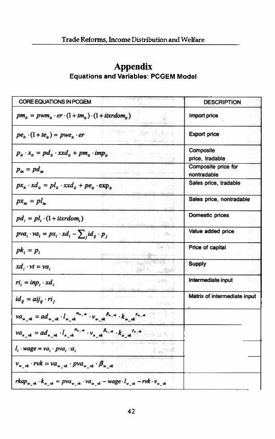
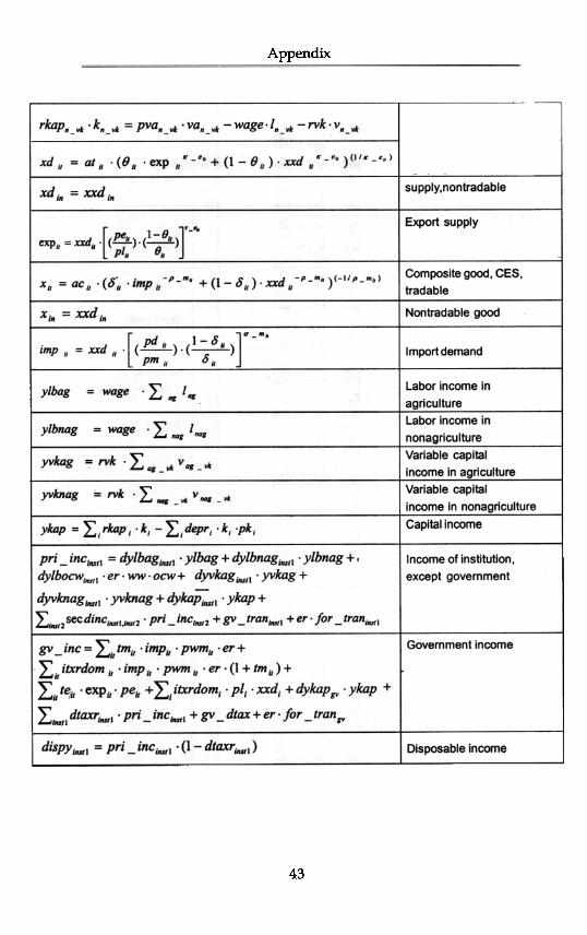
A computable general equilibrium (CGE) model, calibratedto Philippine data using the official 1990 SAM, was employedto analyze the effects of trade reforms on income distributionand welfare. The model is called PCGEM, whose complete setof equations is presented in the Appendix.

PCGEM has 34 production sectors, seven of which compriseagriculture, fishing and forestry. There are 20 subsectors withinthe industry sector, including utilities and construction. Theservice sector is composed of seven subsectors. The modeldistinguishes three factor inputs, namely, labor, variable capital,and capital. Variable capital, which generates mixed income,is an important feature of the model because, as discussedearlier, it is a major source of income of households in the lowerdecile groups. It is a major factor in agriculture, particularly inmajor crops such as palay and corn that are critical to thelower income groups. Variable capital is likewise a major factorin livestock and poultry and fruits and vegetables. Labor isassumed mobile across sectors. For lack of formal modeling ofthe variable capital, it is also assumed to be mobile acrosssectors. Capital, however, is fixed in each of the industries.

Except for capital, there are no restrictions on quantitiesand prices. Prices vary to clear all the markets. Householdsare grouped in decile.

The simulations conducted in the paper involve changingthe tariff rates of the industries. Compensatory taxes such a,schanges in indirect taxes and income taxes were also includedin the simulations. Refer to Figure 1 for the basic pricerelationships in the model.

Output price, px, affects export price, pe and local prices,pl. Indirect taxes are added to the local price to determinedomestic prices, pd, which together with import price, pm,

20

Model Description

Figure 1. Basic Price Relationships in PCGEMX

will determine the composite price, p. The composite price isthe price paid by the consumers. .

Import price, pm, is in domestic currency, which is affectedby the world price of imports, exchange rate, er, tariff rate,tm, and indirect tax rate, itx. Therefore, the direct effect oftariff reduction is a reduction in pm. If the reduction in pm issignificant enough, the composite price, p, will also decline.

The value added relation as well as the underlying utilityfunction of consumers is assumed Cobb-Douglas. Armington-CFS(constant elasticity substitution) function is assumed between localand imported goods, while a CET (constant elasticity oftransformation) is imposed between exports and local sales. TheArmington and the CET elasticities are presented in Table 15.

In terms of model closure, the current account balance, aswell as the exchange rate, is fixed. Total investment in real

21


terms and total government consumption, also in real terms,are both held fixed. Total investment and total governmentconsumption in nominal terms vary. Their respective pricesvary as well. Transfer within government, which captures theremittances of government corporations to the nationalgovernment, is endogenous.

22

v

Simulation Results

Two scenarios were analyzed in the simulation exercises.The first involved complete elimination of tariff. The secondinvolved actual change in tariff.

1. ZERO- YT AX -this is a scenario of complete eliminationof tariff in all sectors, that is, tm in Figure 1 in all sectors is setto zero. The compensatory tax mechanism is additional incometax, implemented in the model through the following

equations:

la. dpyh = Yh*(l-ydtaxh*(l+ntaxr))lb. ntaxr = ntaxf (LhYh)lc. yg' = yg + ntax

where dpyh is disposable income of household h; y h is income;ydtaxh is direct income tax; ntaxr is additional income tax rate,and yg' is government income augmented by additional taxrevenue ntax.

2. ACTU AL- YT AX -this is similar to the previous scenarioexcept that sectoral tariffs were reduced usirig actual changeiri tariff withiri the period 1990-2000. That is, the calibratedtariff rates iri the model were updated iri the simulation runusirig the actual nominal tariff change calculated from the peaktariff rate to the lowest rate withiri the period. For example, irithe case of palay and corn, the change iri the nominal tariffrate from the peak in 1996 to the lowest rate in 2000 wascalculated using a simple growth formula and applied toupdate the calibrated tariff rate iri the model.

23


The compensatory tax mechanism is the same as theprevious one.

Some of the base values of variables were presented in thetables discussed in the preceding sections. In Tables 12 to 14,other relevant base values of variables are presented. Thesevalues are important in the comparative analysis of thesimulation results given below.

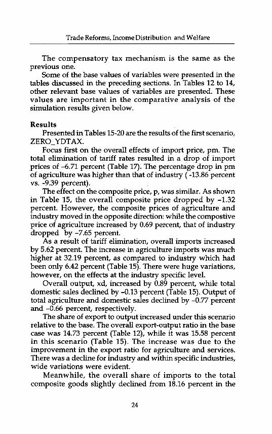
ResultsPresented in Tables 15-20 are the results of the first scenario,

ZERO_YDTAX.Focus first on the overall effects of import price, pm. The

total elimination of tariff rates resulted in a drop of importprices of -6.71 percent (Table 17). The percentage drop in pmof agriculture was higher than that of industry (-13.86 percentvs. -9.39 percent).

The effect on the composite price, p, was similar. As shownin Table 15, the overall composite price dropped by -1.32percent. However, the composite prices of agriculture andindustry moved in the opposite direction: while the compostiveprice of agriculture increased by 0.69 percent, that of industrydropped by -7.65 percent.

As a result of tariff elimination, overall imports increasedby 5.62 percent. The increase in agriculture imports was muchhigher at 32.19 percent, as compared to industry which hadbeen only 6.42 percent (Table 15). There were huge variations,however, on the effects at the industry specific level.

Overall output, xd, ihcreased by 0.89 percent, while totaldomestic sales declined by -0.13 percent (Table 15). Output oftotal agriculture and domestic sales declined by -0.77 percentand -0.66 percent, respectively.

The share of export to output increased under this scenariorelative to the base. The overall export-output ratio in the basecase was 14.73 percent (Table 12), while it was 15.58 perceI:ltin this scenario (Table 15). The increase was due to theimprovement in the export ratio for agriculture and services.There was a decline for industry and within specific industries,wide variations were evident.

Meanwhile, the overall share of imports to the totalcomposite goods slightly declined from 18.16 percent in the

24

Simulation Results

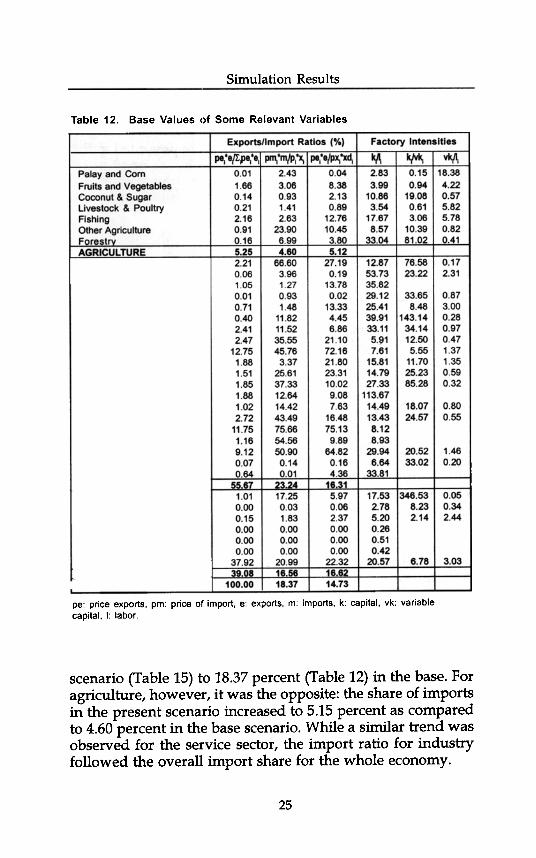
Table 12. Base Values of Some Relevant Variables

Exports/Import Ratios ("/0) Factory Intensities

kA kIvkI V~I0.15 18.380.94 4.22

19.08 0.570.61 5.823.06 5.78

10.39 0.8281.02 0.~1

~pe:e,l Jrn. 'm/p,'Xj I pe,.e/pXj 'xd,0048.382.130.89

12.7610.453.805.12

2.83

3.99

10.86

3.54~'17.67 8.57

33.04

Palay and Corn

Fruits and Vegetablesi Coconut & Sugar

Livestock & Poultry

FishingOther AgricultureForestrAGRICULTURE

0.011660.140.212.160.910.165.25 I

2.210.061.050.010.710.402.412.47

12.751.881.511.851.881.022.72

11.751.169.120.070.64

55.671.010.000.150.000.000.00

37.92

2.43

3.060.931.412.63

23.906.994.80

66.603.961270.93148

11.82I11.52

35.5545.76I

3.3725.6137.3312.6414.4243.4975.6654.5650.90

0.140.01

23.2417.250.031.830.000.000.00

20.99

12.8753.7335.8229.1225.4139.9133.115.~17.61

15.8114.7927.33

113.6714.4913.438.128.93

29.946.64

~_1-

76.5823.22

33.658.48

143.1434.1412.505.55

11.7025.2385.28

0.172.31

27.190.19

13.780.02

13.334.456.86

21.1072.1621.8023.3110.029.087.63

16.4875.13

9.8964.82

0.164.36

0.873.000.280.970.471.371.350590.32

18.0724.57

0.800.55

20.5233.02

1.460.20

16.315.97 17.53 346.530.06 2.78 8.232.37 5.20 2.140.00 0.260.00 0.510.00 0.42

22.32 20.57 6.7816.6214.73

0.050.342.44

MiningRice & Corn MillingMilled SugarMeat ManufacturingFish ManufacturingBeverage & TobaccoOther Food ManufacturingTextile manufacturingGarments & LeatherWood ManufacturingPaper & Paper ProductsChemical ManufcturingPetroleum RefiningNon-metal manufacturingMetal ManufacturingElectrical Equipment Mnfg.Transport & Other Mach.Mnfg.Other ManufacturingConstruction

I Electricity. Gas and Wateri INDUSTRY

Financial SectorPrivate EducationPrivate HealthPublic EducationPublic HealthGeneral GovernmentOther Services ~SERVICES !

I TOTAL -I

3.03~ I 16.56 I

100.00 I 18.37 I

pe: price exports, pm: price of import, e: exports, m: imports, k: capital, vk: variable

capital, I: labor.

scenario (Table 15) to 18.37 percent (Table 12) in the base. Foragriculture, however, it was the opposite: the share of importsin the present scenario increased to 5.15 percent as comparedto 4.60 percent in the base scenario. While a similar trend wasobserved for the service sector, the import ratio for industryfollowed the overall import share for the whole economy.

25

U)

Q)..caor.(/)Q

)

E0\J.5"C"0or.Q

)U

)~0~...0U

)Q

)~(ij>Q

)U

)caa3M.-Q

)

:c~

!l21C

'! ~

~

C'!I0;

~Q

)a:>a:>

MO

~N

~"-

0-

~I~ ~

"': "':I

C!

I~

-.tLn<O

-.to

~M

-.t.- 0...

~1

~~

«J;<o;

I~

=

O>

UJc!)1C

>

0: M

M-=

~

i

! I~

~O

! 1'-:1

0; ~

.-M<

Dcx)O

~~

M.-

0~

~

WO

:M

01IG

O

~om

wo

I-""M~

~

~

~ I~

""! ~

~I~

I~

CX

)r-.oC')o

~~

"'N

0...

~I~

~~

~I~

I

21~

,,-:~"!

1~..L!).-O

MO

...NL!)N

0-

!IO

; """: ~ """: 1~

~I'

OO

MO

~N

I().- 0.-

E0...-Q

)--U

)e

~.c.!9

~Q)

Eo

ro.-.c

.~

Co.c

-

8~~

~o~

.: I-

Trade R

eforms,

S"5-co0

OI/)M

ON

O

~M

CD

.-I---O~

MM

N

~

!<D

;"':"':I'-:~N

CD

I---O~

vM.-

0...

26 Distribution

and Welfare

"in'G

)>

<sG

)

E0uc~0~1/1CG

)C

oE0U'CC~:t:.~S0..G

)N0.~~CG

)U~1/1...UG

):t:wG

)'C~~I()~G

)

:c~

000000000000000000

.~~

~~

~~

~~

~~

~~

~~

~~

~~

q~~

~~

~~

~~

~~

~~

~~

~~

8oo~

oo~oooooooooooo

~~

~~

~~

~~

~~

~~

~~

~~

~~

~~

N~

~~

OO

OO

OO

OO

O~

~~

~O

O

27

'~'8 I,:,i~!~

~~

000

~~

~~

8~~

~~

~~

~~

~~

8~~

~~

~

~~

-OO

ON

~O

ON

-O-O

-~M

~O

OO

000

~

~"C

I'~!

~ ~

~ ~

~ ~

g ~ ~

~ ~

~!

~ q ~

~ ~

~ ~

~ ~

~ ~

~ ~

~ ~

~ ~

~ 8 8 8 q ~

~I%

Or--N

O~

~",in~

o~o~

...<o~

~~

~~

O)a>

~~

~!B

°"'~<

OO

NO

OO

~~

~-

.0>,

U

...~g.

a.

u~

'j: gj

-E,"1~~

~~

~~

~~

~$~

~~

~~

~~

~~

~~

~~

~~

~~

~q~

~~

~888~

~~

~

e"'N~

~N

~<

O-'!B

"'N~

~<

O~

~~

N~

~~

~~

~~

2°o~~

o~ooo~

~~

~

, a.

eg. iI)"t:0

-a.~

"

-0>.=I~

~q ~

~ ~

~ ~

~ ~

~ ~

8 q ~ ~

~ ~

~ ~

~ ~

~ 8 ~

~ ~

~ ~

~;~ ~

8 ~ 8 8 8 ~

~~

~

~

0 ~ 0 0 ~

0 0 ~ ,~

O ~

0 0 0 N N

~ ~

~ ~

~ ~

N,~

~ a>

0 0 00000

0 ~g

y."

~

~

'" "t:

.c. ~

0

In' a.

-."I! g. 0>

:; ->

.¥'j:

o~In-

O>

ue

u~,

.~ I/)

I~[~

~ ~

~~

~

~,

~8~

~

~~

~

~ ~

~~

~~

~

~~

~8~

a ;~

8 ~

8 8 8~

~ ~

~

~ooooo~

c~a>

~O

OO

ON

"""O~

r--~~

a>o)o)"'O

a~N

Ooooo~

~g

~o

e ~

.."C

, I/) "C

e "t:o

g. 01/)a.-

-E~

~

.-.9--..~~

E

o

'~~

~~

~~

~~

~~

~~

~~

~~

~~

~~

~~

~~

~~

~~

~E

~~

~~

~~

~~

~

~~

I~~

"'~"""~

O

~N

ON

O~

"'O~

OO

~O

OO

OO

O~

NM

"'~O

NO

"'~~

g a...

I", ~

E

-~

.-5-

'" '0 :;

>

0>

0g.

-.,-.~

tU

qq a.:g

og

..~

E

-ij.a.x

--ij-ij00

~8

q.., "co)

00 tU

o>

0>'"

~

I/)

~8.

>

E..0tU

U

>..X"C0>

..;;"C

~

"Ca.tU

-~0>

0~

-~

o>

0>-u0

.~s.

0> a.

~

u ..

01 .~

~.~

x C

0101'

a.

'c '"

c~.c

~a.

-~

01 C

~

U

.,

'" -U

c" -"

:>

(V

0>.,

0101

8u O

Ic

~ C

I~ C

~

01 C ~ 01 :>

->

u-01

co Q

)CU

"OIU

C~

C

~

~.~

~~

~

Q)

~

§CU

'5§.cceu5.et:t=Q

;t: ~

a. a.

"co- ~

-"ccoc

-"a.""t:""g..c"~

'"5 c

..E

"OI-"

~

u".acoumu~

"~cu--u

0- 0

'" 0>

0>

~~

~~

a

EiU

~i~

~~

~~

~~

&~

~"tJ~

~5

>~

~~

~~

J~U

I E

~~

~;-11

OI~ 'j

8:!,~

c &~

~!!.~

~B

§S

~B

'6~U

2~

~:m

~£iB

:I:-c?!~

!EE8.

cococ~c

OI~

~

LL.,

~

Q)

co. _InO

.,.,uu

i~~

~~

gLL j~

jl~ig~

J~~

~~

jl~~

~~

!~~

~~

~~

jgi~ ~~


Table 15 continued

-Volume Changes6m,(%) 6xxd %140.93 -2.613321 00.07

517.66 00.41106.66 00.5223.~ 0.515.65 0567B4 0.69

32.19 00.66-1.06 00.5911.51 026

70223 0.6179.94 0.5567.67 05636.14 2B45.60 1.66

20.72 11.1616.54 122629.56 1.46

3.04 00.932.66 121

35.65 -2.566.74 1.434.53 00.635.66 3B53.12 -2.556lJ3 2270.05 0330.00 1316.42 1.00

0023 00.102.04 1.761.29 1.15

00.5203>

-16.241;YS 1.06

1.22 -14.645.62 00.13

&

-1.57 -127

1.61 1.39-0.94 -3.451.12 0.711.13 0274.05 -4261.39 -0.67

-3.11 -7.04

-4.67 -12.15-O.~ -2.30-224 -3.~-0.75 -2.45-7.13 -12.66-2.40 -3.99

-2.38 -3.63

-4.11 -4.89

-3.01 -4.56-425 -5.84-1.35 -1.35

-1.05 -1.05

00.96 .7.65-0.69 -0.57-0.01 -0.01O~ 0.65

-0.74 -0.74-1.47 -1.47-1.50 -1.50

1.40 1.11o~ 0.57om .1.32

~

Xd% -2.81

00.3400.4200.52 I028

I0540.68 i

.0.71 i

ore i0260.71 I054 I

026 i

2.58 :1.5911.7022.63

1.77.0.451.31

-2.37

1.7200.2214.37-2.15

4.04I0.33 1.33

2.33 ,

00.08I1.78 1.14

00.52oX!

-18.24o~ I

-1:16 I

0.89 i

Palayand ComFruits and VegetablesCoconut & SugarLiwstock & PoultryFishingOther AgricultureForestrvAGRICULTUREMining'Rice & Corn MillingMilled SugarMeal ManufacturingFish ManufacturingBeverage & TobaccoOther Food ManufacturingTextile manufacturingGa~ts & LeatherWood ManufacturingPaper & Paper ProductsChemcal ManufcturingPetroleum ReliningNon-metal manufacturingMetal ManufacturingElectrical Equipment Mfg.Transport & Other Mach. Mfg.Other ManufacturingConstructionElectricity, Gas and WaterINDUSTRYFinancial SectorPrivate EducationPrivate HealthPublic EducationPublic HealthGeneral GovemrT81tOther Services

I ~~~:CEStm: tariff rate; pva: price of value added; va: value added; pm: price of imports; m: imports;pe: price of exports; e: exports; pd: domestic price; p: composite price; px: price of output,x: composite good; xd; total output; xxd: output sold domestically

There were relatively few noticeable effects on the structureof the economy as a result of a complete elimination of tariff.For example, in the structure of imports, the share of agricultureimports to the total increased from 3.53 percent in the base(Table 6c) to 4.08 percent in the present scenario. The share ofindustrial imports, however, declined from 66.19 percent inthe base to 64.83 percent, while the share imports in the servicesector increased from 30.28 percent to 31.10 percent. Asexpected, there were no changes in the structure of exports.

In addition, there were small changes in the structure ofvalue added. The value added share of agriculture decreased

28

Simulation Results

slightly from 23.3 percent in the base (Table 4) to 23.24 percentin the present scenario (Table 15). Similarly, the share of servicesector value added declined from 45.3 percent to 44.65 percent.However, the share of industry value added increased from31.5 perc~n~in the base to 32.11 percent.

Wages, w, declined by -0.60 percent, while the price ofvariable capital, rvk,'fucreased by 3.58 percent (Table 16). Theincrease in the price of capital, rk, in all the agriculturesubsectors was consistently below the increase in the price ofvariable capital. As a result of these changes in factor prices inagriculture, capital/labor ratio in all the subsectors declined,the capital/variable-capital ratio increased, and the variable-capital/labor ratio declined (Tables 12 and 16). This meansthat labor was used relatively more than the two factors inagriculture under the present scenario.

Mixed results were found in the case of industry, however.There were subsectors.where the increase in rk was lower thanthe increase in rvk. In those subsectors, just like in agriculture,a similar factor movement was realized wherein the utilizationof labor increased relative to the other factors. However, therewere industry subsectors where the increase in rk was a lothigher than the increase in rvk. This was the case in beverageand tobacco, other food manufacturing, textile manufacturing,garments, wood manufacturing, chemical manufacturing,nonmetal manufacturing, electrical equipment, othermanufacturing, and utilities. In these subsectors, factor shiftsmoved in favor of labor and variable capital, except in thoseindustries that were not employing variable capital. However,in subsectors where rk declined, such as petroleum andtransport manufacturing, factor movement was observed tofavor capital.

The same mixed effects were observed under the servicessubsectors.

There were impacts observed on indirect taxes even thoughindirect tax rates of industries were not changed under thisscenario (Table 17). These effects were due to changes indomestic sales, local prices, imports and tariff rates. Indirecttaxes on agriculture and services increased, which resulted inpart from the increase in the domestic price of locally soldagriculture goods. Since pd of agriculture increased by 1.63

29

Trade R

eforms, Incom

e Distribution

and Welfare

~ I~ ~

~~

I:j~&

1II~

~$~

$~~

1D:~

ai'85!~~

~I:::~

Iq1D:I:jII

fd:1D:~

~~

~l

~-

ON

ON

(')NN

O

(,)NN

N;:"";::!:!"'O

"'~"'O

~~

;:O'"

qN('),;-q~

c

~ ~

~ ~

~ ~

~II~

~ ~

~ ~

~~

~~

~~

~~

~ ~

~ ~

~ ~

~II~

~~

~~

~ ~

i:)

:&7,

'oc

~:,

, a""0>

;u.~C

o

~~'s.~:,;.

~'s.~Q

):c.!2ro>"0.~50

~~'s.01UQ)

:c.!2ro>:,;.>;JjQ

)Q

)

~~0.0.!Y.

~0

30

~ ~

~II~ ~

~ ~

~ ~ ~

~ ~

~ ~

~ ~ ~

~ ~

~W

I~I~

~~

j~!p; ~,qqq

qqqqqqqqqqqqqqqqqqqq tqqq'T

T'1"

Sim

ulation Results

1°1

~ ~

~~

;::r;;;oU

i~N

Ui6;;j;;;

!I~

~~

~

~

o."o~q","1~

~..."i;;;"""",,~

""'i..,,,:~

m~

~~

o~~

o~o~

o~o~

-~~

~-~

~~

!~

:9:11 ~ ~

~ ~

~

~

o",o~...o

..~

,_.",

~~

~O

i~a~

;;d~',::o~

o~]

8Ui~

°"'°';~

~

,.-'~

.c:~

o

~8!~

6I0"'0-

~6';"d~

-u;-Q

)>

<~Q

)

E0uc~0~II)cQ)

Co

E0U"CCCO

==

.~~0...Q)

N0.~CO

CQ)

U~II)

UQ)

......WC0Q.

E~II)c0U,..:...Q

)

::c~

'8oU>

o-...

';:~.;::o"'oo..:

., ,'"

":000-000-

~I ~

~~

~6do';;~

od-

"'1

'8~

0

~;: ~

~~

~~

8I~

0100"'100

~-UlU

I--N-

-a- "I ., "1 '" "I '"

g. """0--000

~-~

N~

~d~

odoood~ood

~"'fD

...","'om~

~q;:"",~

~;

':;f1~~

~;;: ~ ~

:t '1 Y ;;:~

I

~~

'aj~~

I~,,?

~ ~

l'a>O

)~a;~

.,;a;cO~

-;-')'.,.,,;>,;-'

" -,

--""':M

M,",N

~O

q~o;'

! I il~Jm

~:£~

~

~ ~ ~ ~ ~ ~ ~ ~ ~ ~ ~ ~ ~; ~I~

I~

~ ~ ~ ~ ~ ~I~

I~Id~N.P

-

.~"0'":I::I:~.P

-'"Q

)"0J::I:

$iJ.~

on C

I C

I

U~

§

~£

:J ..

O~

~!~

~

01CC~C

I C

I5;

c:=

c:

~

£E

ro~O

Clc:

U,~

O

J

~:=

Ero"

B~

-tU-

,.Q)~

~~

I!!~

31

onQI

~~

2:' Q

I"'m

'" ~

g 5J. g" '-~

~u>

'" a

"O"O

~~

c

C

c-i'i 01

m

mE

501<>

-ono

_c~m

- on-Q

I-

2-uQI':.:

m

0>'"-

"-LLU::Ji.:O


percent while indirect taxes increased by 3.11 percent, the localprices of these goods before taxes must have declined.

In industry, the effects were varied across subsectors, buton the whole the average price of domestically produced goodssold locally declined by -0.96 percent while indirect taxesdecreased by -1.41. This indicates that local prices before taxesmust have increased.

The structure of household consumption is shown in Table10 for the base case and in Table 17 for the present scenario.Generally, one can observe that across household groups therewas a decline in the share of agriculture-based consumptionand an increase in the share of industry-based consumption.There were mixed effects on service sector-based consumptionacross the different decile groups.

Because of the decline in wages, total labor income declinedby -0.52 percent (Table 18). However, there were interestingdifferentiated effects across household groups. One can observethat labor income improved for the first decide up to the fourth,despite the decline in wages and agriculture output, xd. This effectcan be attributed mainly to the impaC\ on the relative factor pricesin agriculture that allowed for factor shifts in favor of labor.

Furthermore, one can observe that the increase in laborincome for the first four deciles became smaller as one movedto a higher decide. Labor income for the first decile increasedby 1.02 percent and for the fourth decide by only 0.26 percent.This is mainly because compared to the higher income groups,lower income groups are heavily dependent on agriculturelabor as source of income (Table 9).

Meanwhile, labor income from the fifth to the tenth decilesdeclined, and the magnitude of the drop was increasing asone moved to the higher income groups. Again, this can beattributed to the structure of labor income for these groups.Since total labor supply is assumed fixed during the simulation,the improvement of labor utilization in agriculture would implysome movement of labor from nonagriculture to agriculture.This, together with the decline in wages, resulted in a reduction,albeit small, in labor income for these groups.

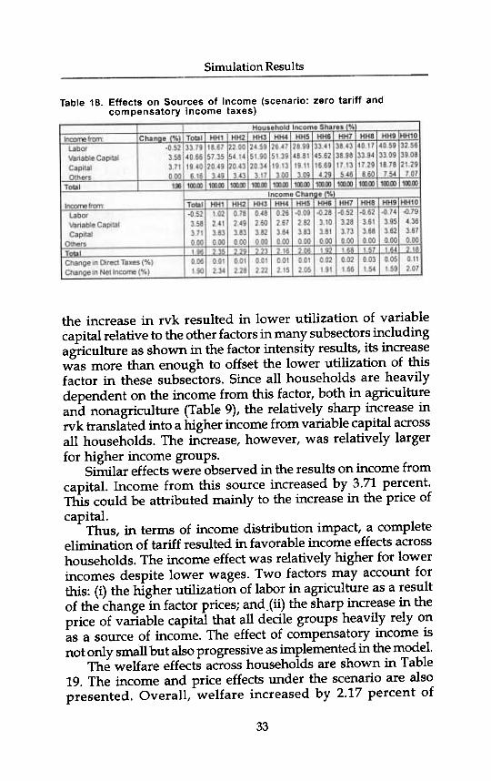
As shown in Table 18, income from variable capitalincreased by 3.58 percent; which could be attributed mainlyto the increase in the price of variable capital, rvk. Although

32

Simulation Results

Table 18. Effects on Sources of Income (scenario: zero tariff andcompensatory income taxes)

the increase in rvk resulted in lower utilization of variablecapital relative to the other factors in many subsectors includingagriculture as shown in the factor intensity results, its increasewas more than enough to offset the lower utilization of thisfactor in these subsectors. Since all households are heavilydependent on the income from this factor, both in agricultureand nonagriculture (Table 9), the relatively sharp increase inrvk translated into a higher income from variable capital acrossall households. The increase, however, was relatively largerfor higher income groups.

Similar effects were observed in the results on income fromcapital. Income from this source increased by 3.71 percent.This could be attributed mainly to the increase in the price of

capital.Thus, in terms of income distribution impact, a completeelimination of tariff resulted in favorable income effects acrosshouseholds. The income effect was relatively higher for lowerincomes despite lower wages. Two factors may account forthis: (i) the higher utilization of labor in agriculture as a resultof the change in factor prices; and.(ii) the sharp increase in theprice of variable capital that all decile groups heavily rely onas a source of income. The effect of compensatory income isnot only sIruill but also progressive as implemented in the model.

The welfare effects across households are shown in Table19. The income and price effects under the scenario are alsopresented. Overall, welfare increased by 2.17 percent of

33


disposable income, mainly due to the increase in income andin the reduction of prices resulting from the total eliminationof tariff. The increase in welfare was slightly higher for thelower income groups.

The macroeconomic effects are shown in Table 20. One shouldrecall in the simulation that the model was made with the followingassumptions: (a) total government consumption is fixed in realterms; (b) total invesbnentin real terms is also fixed; and (c) currentaccount balance is fixed. The first two assumptions would notallow fqrreal changes in the totals of these two demand variables,but would only consider reallocation across sectors as a result ofchanges in relative prices. The third assumption would not allowfor changes in foreign savings.

What would be the impact of using actual tariff changesinstead of a complete elimination of tariff? This is scenarioACTUAL_YTAX. The results are presented in Tables 21 to 26.

The change in tariff rates is shown in Table 21. The averagereduction in agriculture was -56.5 percent and in industry -74.3 percent. In agriculture, the tariff in palay and corn hadthe smallest reduction, owing to the tariffication of QRs in themid-1990s. In industry, sugar milling and palay and cornmilling had relatively smaller tariff reduction.

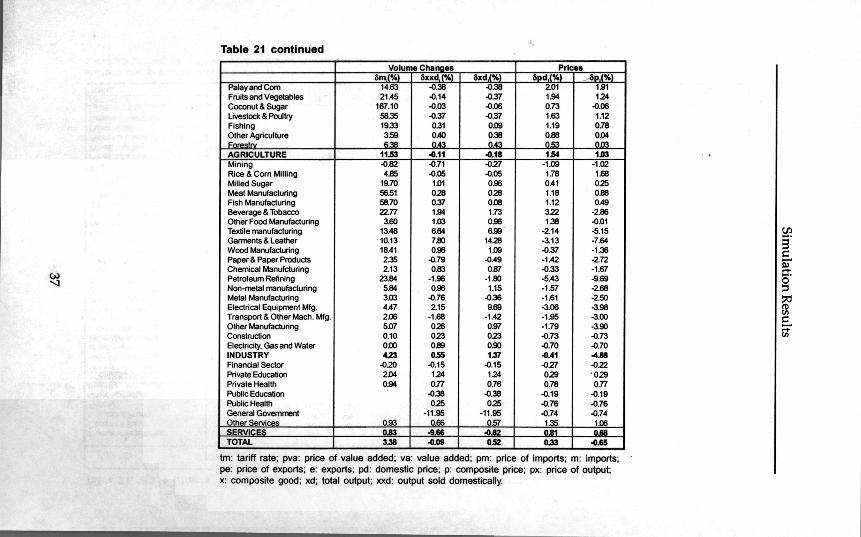
Generally, in terms of direction of change, this scenario issimilar to the first one, except that the magnitude of change issmaller. This is due to a less drastic cut in tariff as compared tothe first one, which is a complete elimination of tariff. Thedrop in the composite price was -0.65 percent, with industryhaving the largest at -4.88 percent. The drop here can beattributed to the drop in import prices (Table 23).

The direction of the change in factor prices had been thesame as in the first simulation. However, the changes wererelatively smaller. For example, wage declined-by only -0.06percent. The price of variable capital increased by 2.96 percent.Factor intensities changed accordingly.

Because of a much lower decline in wages as compared tothe first scenario, the decline in the overall labor income hadalso been smaller. Moreover, because of relatively larger laborshifts in agriculture, the increase in labor income for the lowestincome brackets had also been much higher than in theprevious set of results.

34

Simulation Results

Table 19. Income and Welfare Effects (scenario: zero tariff andcompensatory income taxes)

Table 20. Macroeconomic Effects (scenario: zero tariff andcompensatory income taxes)

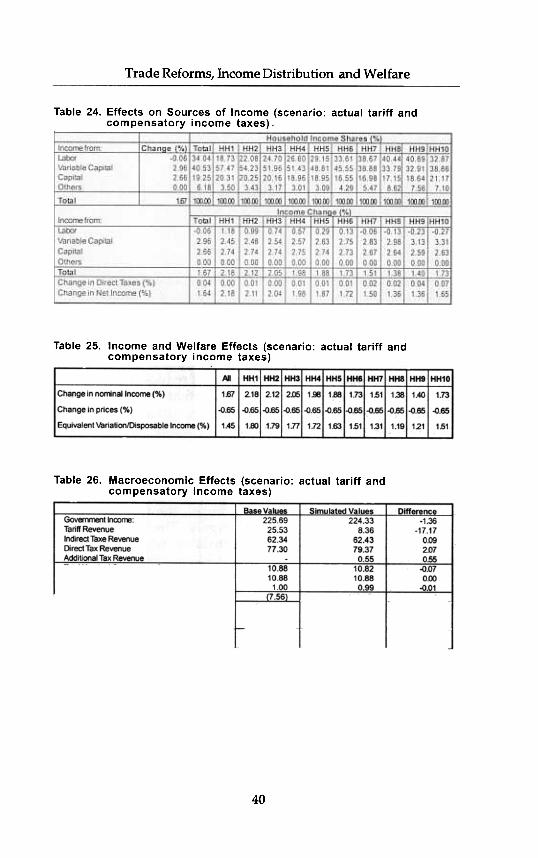
The impact on income across households, however, wasdominated by the increase in both the price of variable capitaland of capital. Since all household groups are largelydependent on income from variable capital, either inagriculture or in industry, the large increase in its price had afavorable effect on their respective incomes. Thus, the actualreduction in tariff resulted in a favorable income distributioneffect.

The impact on welfare is shown in Table 25. Again, the changein tariff using actual reduction results was found to be welfare-improving. Total welfare improved by 1.45 percent of disposableincome. There were no wide variatioRS in the welfare effects acrossdeciles. The effects on the lower income groups were slightlyhigher than on the higher income groups. The welfare effectswere due to higher income and lower prices.

The macroeconomic effects of the present tariff scenarioare presented in Table 26.

35

Trade R

eforms, Incom

e Distribution

and Welfare

;i'l

~'O

iSj~

~!6~

:"f- N

-ON

N-C

'

ocT~~

~~

~~

~

~ ~

~ ~

~ ~

~~

N

NN

NN

NN

00

$ ~ $$ $$ $$ ~

~.~

~~ ~

~~

~ ~

~ ~

N~

NN

NN

NN

NN

NN

NN

NN

NN

NN

$$$$$$$N

NN

NN

NN

"6Q)

.25-

-tro'5.m()

:;;.

S.a.m()Q

):0.~ffi>"6.~5-

:;;.~ro.5-

~Q)

:0.~ffi>:;;.>in"Q

)O

Jm~~'0.c.!Y

o

38

~s!~

~I:j~

~O

i~f)j$~

~~

I:j~~

I;!~'6I

II~

~~

~~

'.;;::Sq

~~

NN

~~

O~

MO

MO

MO

~N

MO

Mq

NN

qO

NM

~N

')'

~.

";-

Sim

ulation Results


Table 24. Effects on Sources of Income (scenario: actual tariff andcompensatory income taxes)

Table 25. Income and Welfare Effects (scenario: actual tariff andcompensatory income taxes)

Table 26. Macroeconomic Effects (scenario: actual tariff andcompensatory income taxes)

Total Nominal Government ConsurT1>tionTotal Real Government ConsurT1>tionPrice Index of Total Government Consuorotion

GovemmentBalance (12.37) -4.~Total NorTinallnvestment 2,601.63 2,576.40 -25,24Total Real Investment 2,601.63 2,601.63 0.00Price Ind x of Total Investment 1.00 0 99 .Q 01Balance of Trade (59.65) (59.65) 0:00CurrenlAccountBalance 51.71 51.71 0.00

40

VI

Conclusion

Results of the study show that the reduction of tariff ratesis welfare-improving across household groups, although thesize of the improvement is not too significant (only about 2percent of disposable income).

The forces at work are both the improvement in incomeand the reduction in prices of commodities and services.Although wage declined as a result of tariff reduction, changesin factor prices resulted in factor shifts that favored labor,especially in agriculture. Furthermore, the price of variablecapital and the income derived from it, officially called mixedincome, improved significantly during the tariff reductionsimulations. Since all household groups are sourcing theirrespective incomes significantly from this factor (mixed incomein agriculture for lower income groups and mixed income innonagriculture for higher income groups), th~ increase wasfound to benefit all groups almost evenly. The treatment ofvariable capital in the model is similar to labor, which is mobileacross sectors.


AppendixEquations and Variables: PCGEM Model

DESCRIPTIONCORE EQUATIONS IN PCGEM

pmit = pwmit .er.(l +tmit).(l+itxrdomit) Import price

Export pricepeil .(1 + teil) = pweil .er

Composite

price, tradablePit -XiI = pdi, -xxdil +pmil .imPi'

Composite price for

nontradablePill =pd;"

Sales price, tradablePXjt .xdjt =pljt .xxdiJ +peiJ .expiJ

Sales price, nontradablePX;n = pl;n

Domestic pricespd; = pi; .(1 + itxrdom;)

Value added pricePva. .va. = px. .xd. -~ id ij .p .I I I I £...j' }

Price of capitalpkj =Pj

Supplyxd; .vt = va;

Intermediate input

Matrix of intermediate input

ri; = inp; .xd,

idy = ail!! 'riJ

Value added, sectors wI

variable capitalaw_..vaw_vk = adw~vk .lwvk v

~

.8... kw '* -.w vk

Value added, sectors w/o

variable capital

Demand for labor

a... 11,_.. .kva..vk = ad._vk o/._Vk v.~vk n~vk

j .wage = vaj .pvaj .a,

Demand for variable capitalVw_vi .rvk = yaw_vi .pvaw_vk .Pw_vk

Returns to capital in sectors

with variable capital-rvk. vrkapw_vk .kw_w = pvaw_w .vaw_vk -wage./w_w

42

Appendix

Returns to capital in s:~1without variable ca ital

Composite supply, CET,tradable

rkap"vk .k" vk = pva" vk 'va"vk -wage'/,,_vk -rvk,v,,_vk

xd;, = at II .(fJ;/ .exp ;/ K _0. + (1 -fJ;1 ) .xxd ;/ K -"" )(I/K _0.)

supply,nontradablexd in = xxd in

Export supply[ e 1-0

] '-" expo =xxd.. (E..!!-).(--D-)

pl. O.xxd -p_m, )<-llp_m,>

/I(~.. -p" ( ~ xl,=acl'. UI,.lmpi' -'+ i-uil

Xi. = xxd i.

Composite good, CES,tradable

Nontradable good

Import demand

ylbag L ag lag= wage

LnDglnDgylbnag = wage

yvkag = rvk 'Lag_vkVag_vk

yvknag = rvk "L- vkV...g vk

Labor income in

agricultureLabor income in

nonagricultureVariable capitalincome in agriculture

Variable capital

income in nonagriculture

Capital incomeykap =L;rkap;okj-L;deprjokj'pk;

Income of institution

except government

pri -incins/l = dylbagins'l .ylbag + dylbnag;ns/l .ylbnag + I

dylbocwins/l .er. ww. ocw + dyvkag ins/I' yvkag +

dyvknag ins/I' yvknag + dykah/l .ykap +

Linsl2 sec dinCinsl I,lnsl 2 .pri -incins/2 + gv -tranins/l + er. for -trani""1

Government incomegv_inc=Ljttmjt .imPit .pwmit .er+

Lititxrdomit .imp it .pwmit .er.(l+tmit)+Litt~it .exPit. peit + Liitxrdomj .plj .;xxdj +dykapgy .ykap +

Ltnst,dtaxriMtl .pri_inCtMtl + gv _dtax+ er. for _trangy

dispy instl = pri -inCinstl .(1- dtaxr inltl) Disposable income

43


Savings of institutions

except government-pay ins' I

pri -save'nsll = pri -inc;nsll .(1- dtaxr;I."I)-

~ Pri cc I .P -L.;nsl! -"'" ,I ,

L""'2sec dinc '",'2,;",'! .pri -inc;nsl! -er. for

int--:-;;-L .id ;,1.I

pri_CCinstl.i =dCcmtillstl.i -apci/!Stl-disPYillstl

inv i .Pi = dinv i .(tinv - chstk j .P j)

Intermediate demand

Consumption of institutions

except governmentSectoral Investment

L..j

Balance of paymentscab = ~ (pwmil oimp" -pweil oexPi')- wwoocw+-.!.-o wage 0 for _lb+L..u er

Linstfor -paYinst -Linslfor _traninSI

Total Investment

equals total savingstinv = Lwtlpri_save;lUJl +gv_save+caboer+L;depr; .k; .pk;

lb = L Labor market equilibriumsup lbag + sup lbnag + for

I

Variable capitalI

equilibriumsup vkag + sup vknag -~ V

-L..wvk .'_vk

Xalxgv-sev = int alxgv-se + Linstl pri -CC alxgv-se,instl +

gv -CC alxgv-se + inValxgv-se + chstk alxgv-se

Product market

equilibriumexcept in general

government sectorWalras lawwalras = X gv-seo

gv -CC gv-se -inv

-int -~ Prigv -see L ins/ I

gv-se + chstk gv-se

CC gv -se ,ins!

Variables

*** Output and input prices

pm,!) domestic price of imports for tradablespwm(it) world I?rice~ of imports for tradablespe(it) domestic prIce of exportspwe(it) world prices of exportser exchange rate~~ composite pricesPU(J) domestic pricespl(i) domesti.c prices without domestic indirect taxespx(i) sales prIcespk(;) capital good p~cespva. value added prIcespin~ex price index also called GDP deflatorwage average wage ratervk average return to variable capitalrkap(i) ~ectoral.return to capitalww mternational wage rate

44

Appendix

--Taxesbn(it) tariff rateste(it) export tax or subsidiesitXtdom(i) domestic indirect tax ratesdtaxr -> direct income tax ratesgv _dtx value of direct income tax on government sector

--Output, value added and trade variablesx(i) composite commoditiesxx~ xd less exportsxd(i) column sums in the SAM less importsva(i) value addedrili)' vector sums of intermediate inputs!a(~ !I18trix of intermediate inputsImp(it) Importsexp(it) exports .

...Factor inputsI(i) demand for la~rv(W vk) demand for variable capitalk(i) -demand for capitalsuplbag total supply of agriculture laborsuplbnag total supply of nona~culture laborocw overseas contract workerssupvkag total supply of variable capital in agriculturesupvknag total supply of variable capital in nonagriculture

.-Income and savingsylbag labor income in agricultureylbnag labor income in nonagricultureyvkag variable capital income in agricultureyyknag variable capital income in nonagricultureykap capital income except governmentpri-;inC(iMt1) ~come of institutionsgv _mc mcome of flovernmentdiS;py (il8t1) disl?osable .mc<?me. of institutionspn_save(inst1) sa~gs of mstitutions except governmentgv _save savmr;s of governmenttinv total mvesb"ble funds equal to total savingsdepr(i) depreciationcab current account balance

...Demandintii)pn_cc(-Li)gv _cc(i)mvchs~(i)

...Transfersfor_tran(iMl) foreign transfers to institutionsfor_pay (iMI) interest payments to ROWgv _tran(iMt1) government transfers to institutionsfor_lb labor payments to foreign labor

...Walras lawwalras w

intermediate demandconsumption demand of institutions except governmentconsumption of governmentsectoral investmentsectoral change in stocks

variable

to capture walras la

45

Date post:	19-Mar-2018
Category:	Documents
Upload:	vuminh
View:	215 times
Download:	1 times

Trade Reforms, Income Distribution and Welfare: The ... · PDF fileTrade Reforms, Income...

Documents