Conference on Systems Engineering Research (CSER’13) Eds.: C.J.J. Paredis, C. Bishop, D. Bodner, Georgia Institute of Technology, Atlanta, GA, March 19-22, 2013.
Trading off Supply Chain Risk and Efficiency through Supply Chain Design
Marc Goetschalckxa*, Edward Huangb, Pratik Mitala aMilton School of Industrial and Systems Engineering, Georgia Institute of Technology, Atlanta, Georgia
The design and management of an effective supply chain is an increasingly complex and challenging task in today’s global and competitive economic environment. In order to remain competitive, the supply chain must be efficient. One way to improve the efficiency is to establish the minimum number of facilities to ensure the satisfaction of the customer demand. Because of the economies of scale, establishing the minimum number of facilities minimizes the fixed costs of the supply chain. However, the tradeoff between fixed and variable costs makes it very difficult and counterintuitive to predict the configuration of the supply chain with the lowest total
659 Marc Goetschalckx et al. / Procedia Computer Science 16 ( 2013 ) 658 – 667
system cost. The strategic configuration of the supply chain will remain in place for an extended period of time, often
spanning decades. The future conditions in which the supply chain will have to operate can only be forecasted with a high degree of uncertainty. The uncertainty is in part generated by the fluctuations in value of the supply chain environment such as customer demand, cost of raw materials, cost of energy, and currency exchange rates. A second cause of uncertainty is the possibility of occurrence of singular events such as earth quakes, tsunamis, hurricanes, and other disasters. Because of the tight interlinking of elements of a global supply chain, a disaster in a single country may influence the performance of supply chains all over the world. Companies have been aware of the need for risk management when they pursue optimization of the efficiency of the supply chain (Juttner 2005). Consequently, system engineers designing supply chains will now have to consider the tradeoff between supply chain efficiency (reward) and supply chain risk. The Japanese tsunami disaster during 2011 crystalized the need for the explicit consideration of the robustness criterion. In the future, companies that have spent years making their supply chains leaner may want to increase the inventory in their supply chain to increase its resilience (Economist 2011).
Prior work in the domain of strategic design while considering risk has primarily dealt with either solving the robust optimization problem, in which the risk is minimized, or solving the stochastic optimization problem, in which the expected reward is maximized. Recently there has been a focus on deriving the configurations that lie between the risk minimization and the expected reward maximization configurations. Azaron et al. (2005) solved a multi-objective goal programming model with three objectives: minimization of variance of cost, minimization of expected value of cost, and minimization of financial risk. They generated Pareto optimal configurations by manually changing the goal parameters. However, the generated set of Pareto optimal configurations is not an exhaustive set and there may exist configurations that dominate the configurations obtained. Also manually changing the goal parameters, does not lead to an efficient algorithm. In this work, we present an efficient algorithm that will generate all the Pareto optimal configurations in the supply chain, while considering the risk, modeled by the variance of profit, and reward, modeled by the expected value of profit.
We organize this paper as follows. In Section 2 the robust design problem is defined. In Section 3, we define the mathematical formulation of the robust strategic supply chain design problem. In order to compute the robust strategic supply chain problem efficiently, we prove the equivalency of the mean-standard deviation solution to the mean-variance solution for this problem. In Section 4 we report the numerical experience for a metallurgical supply chain. Finally, in Section 5, we identify several conclusions and directions for future research
2. The Robust Design Problem
2.1. Risk Measures
There are several ways to quantify risk such as variance (Markowitz, 1991), downside risk (Eppen et. al 1989), and maximum regret. In this research, we choose the standard deviation of the scenario profits to quantify risk, which allows for a more intuitive interpretation and comparison between supply chain network configurations. If the standard deviation of the scenario profits is used as the measure of risk then the tradeoff between efficiency and risk leads naturally to the coefficient of variation as the slope of the tradeoff between risk and efficiency. The coefficient of variation is also dimensionless which avoids dependencies on the currency units of the profit and allows for the use of a dimensionless tolerance gap in optimization algorithms.
2.2. Risk curve
Prior research on strategic design considering risk focuses on the continuous decision variables. However, a particular supply chain configuration is modeled by a number of discrete decision variables. A supply chain configuration will realize a profit for each of the possible future scenarios. The distribution of the profits for a single configuration will have a measure of central tendency, typically the mean, and a measure of dispersion. The central tendency measure is used as the efficiency of the supply chain and the dispersion measure is used as the risk of the supply chain configuration which. The dispersion measure used in this research is the standard deviation. In order to
660 Marc Goetschalckx et al. / Procedia Computer Science 16 ( 2013 ) 658 – 667
compare these configurations, the Pareto-optimal configurations are defined as the configurations with the minimized risk for a given expected profit or the maximized expected profit for a given risk. This implies that for a given efficiency or given risk all other configurations are dominated by a Pareto-optimal configuration. By this definition, there may be more than one Pareto-optimal configuration under different given efficiency or risk. Furthermore, the risk and efficiency form a tradeoff, i.e., Pareto-optimal configurations with a higher efficiency or expected value also have a higher standard deviation or risk. Since Pareto-optimal configurations are the configurations with the lowest risk for a given efficiency, there exists no other configuration which has more efficiency and less risk. As a result, the final set of Pareto-optimal configurations is found by the lower envelope of the performance curves of every configuration.
The risk curve is defined as a curve of all Pareto-optimal configurations. We can plot its associated minimized risk or maximized expected value for any given profit or risk. The concept is shown in Figure 1. Each Pareto-optimal configuration has a profit probability distribution created by the various scenarios. Note that the profit distributions of various supply chain configurations are shown in the figure as normal distributions for purely illustrative purposes. The actual distribution of the profit depends on the individual case. In the figure, the supply chain configuration determined for the best-guess scenario, i.e. where each parameter has a single deterministic value equal to its expected value, is shown to be located on the risk curve. This is most likely not true for an actual case. Santoso et al. (2005) reported one two real-world supply chains where the optimal supply chain configuration for the most likely value of the parameters was located inside the efficiency frontier, i.e. it was not a Pareto-optimal configuration and should not be selected.
Var
iabi
lity
ofPr
ofits
(Std
.Dev
.)
Expected Value of Profits
Expected Maximum
Profit
Expected Minimum Variability
Best Guess Maximum
Profit
Figure 1. The Risk Curve of Supply Chain Configurations (Reprinted from “Robust Global Supply Network Design” by the same authors in Information Knowledge Systems Management, Vol. 11, No 1, 2012)
3. The Robust Design Problem Mathematical Formulation
3.1. Notation
Sets and Indices:
661 Marc Goetschalckx et al. / Procedia Computer Science 16 ( 2013 ) 658 – 667
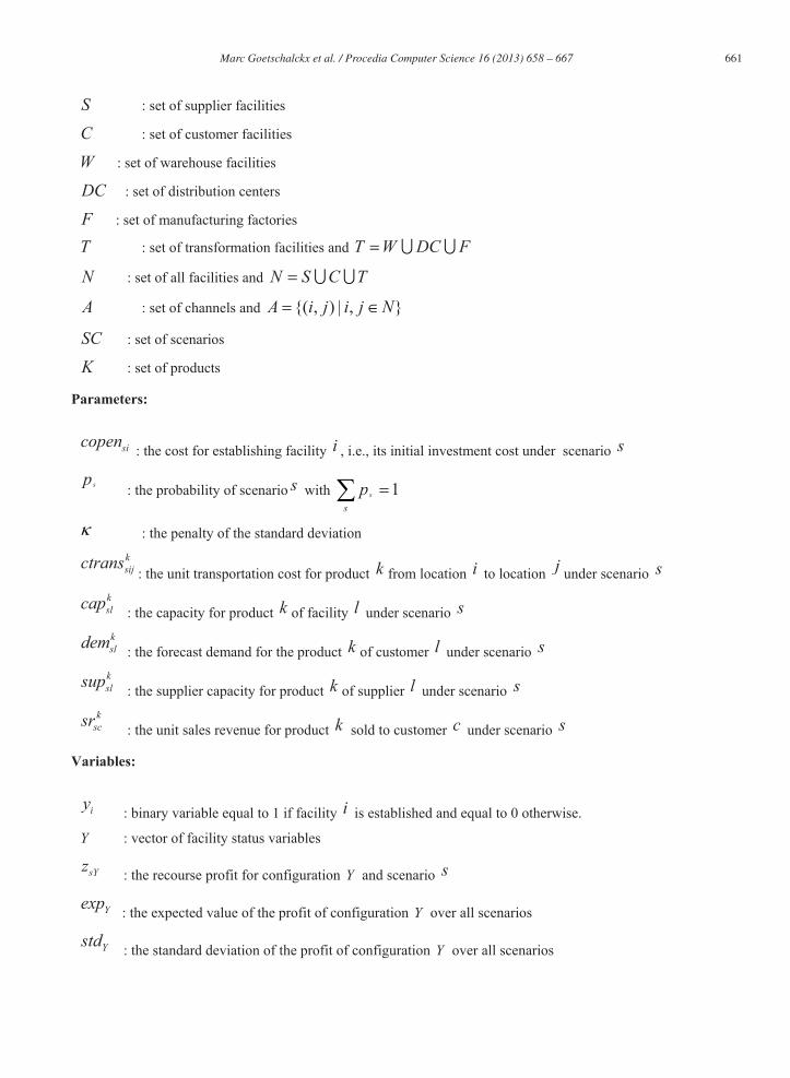
S : set of supplier facilities
C : set of customer facilities
W : set of warehouse facilities
DC : set of distribution centers
F : set of manufacturing factories
T : set of transformation facilities and T W DC F
N : set of all facilities and N S C T
A : set of channels and {( , ) | , }A i j i j N
SC : set of scenarios
K : set of products
Parameters:
sicopen : the cost for establishing facility i , i.e., its initial investment cost under scenario s
sp : the probability of scenario s with 1s
sp
: the penalty of the standard deviation
ksijctrans
: the unit transportation cost for product k from location i to location j under scenario s
kslcap : the capacity for product k of facility l under scenario s
ksldem : the forecast demand for the product k of customer l under scenario s
kslsup : the supplier capacity for product k of supplier l under scenario s
k
scsr : the unit sales revenue for product k sold to customer c under scenario s
Variables:
iy : binary variable equal to 1 if facility i is established and equal to 0 otherwise.
Y : vector of facility status variables
sYz : the recourse profit for configuration Y and scenario s
Yexp : the expected value of the profit of configuration Y over all scenarios
Ystd : the standard deviation of the profit of configuration Y over all scenarios
662 Marc Goetschalckx et al. / Procedia Computer Science 16 ( 2013 ) 658 – 667
ksijx : the flow variable for the product k from location i to location j under scenario s
3.2. Mean-Standard Deviation Robust Design Problem (MSD-RDP)
The Mean-Standard Deviation Robust Design Problem (MSD-RDP) incorporates both the strategic model and the tactical model. Usually, the strategic model has as goal the determination of a robust supply chain configuration that makes the most desirable tradeoff between the long term efficiency and the variability performance of the configuration. In order to determine the profit of each configuration, we model the tactical decisions which are the aggregated flow decisions of the supply chain to evaluate the profit of the future scenario. We assume that the supply chain configuration remains unchanged for all the scenarios. The desired tradeoff between the efficiency, modeled as the expected value of the profit, and the variability, modeled by the standard deviation of the profit, is encapsulated in the dispersion penalty factor . Note that the MSD-RDP is a single stage decision problem just like the inventory newsvendor problem. The decision variables are the configuration of the supply chain, which is comparable to the inventory quantity in the newsvendor problem, and the material flows in the supply chain, which correspond to the sales in the newsvendor problem. All decisions are made at the start of the planning horizon, but the system performance can only be determined after the uncertainty has been resolved.
The Mean-Standard Deviation Robust Design Problem for a given (MSD-RDP( )) can then be written as follows:
Max Y Yexp std (1)
.st
Y s sYs
exp p z (2)
2Y s Y sY
sstd p exp z (3)
( , ) ( , )
k k k ksY sc sic sij sij si i
c C k i c A i j A i Tz sr x ctrans x copen y ,Y s SC (4)
( , ) ( , )
0k ksil slj
i l A l j Ax x , ,k K l T s SC (5)
( , )
k ksil sl l
i l Ax cap y , ,k K l T s SC (6)
( , )
k ksli sl
l i Ax sup , ,k K l S s SC (7)
( , )
k ksil sl
i l Ax dem , ,k K l C s SC (8)
1{ ,..., ,..., }i TY y y y (9)
{0,1}iy i T (10)
663 Marc Goetschalckx et al. / Procedia Computer Science 16 ( 2013 ) 658 – 667
The objective function (1) consists of maximizing the total utility function which is a weighted sum of the expected value and the standard deviation, where the weight of the standard deviation is an input parameter. Constraint (2) defines the expected profit value of the configuration. Constraint (3) defines the standard deviation of the configuration in function of the scenario profits. Constraint (4) computes the profit of each scenario and configuration which is the total revenue minus the investment cost and the flow cost. Constraint (5) enforces the conservation of flow constraint that ensures that the input quantity for each product is equal to the output quantity in each transformation facility. Constraint (6) assures that material will not be transported to a transformation facility if this facility is closed and that the material quantity does not exceed the given capacity. Constraint (7) enforces that a supplier does not provide more of a product than its capacity for that product. Constraint (8) ensures that the quantity of the finished product delivered to the customer does not exceed the demand at this customer. Constraint (9) shows that a configuration is the combination of the decisions to establish the transformation facilities.
From now on we will use the MSD-RDP where the expected value and standard deviation formulas have been directly substituted in the objective function. The MSD-RDP( ) has a square root operator in the objective function and is thus a non-linear non-polynomial mixed-integer programming problem and solving the MSDRDP for a single given may be time-consuming using general purpose non-linear optimization algorithms for realistic problem instances. We will derive the necessary properties for solving this model efficiently in the next section.
3.3. Mean-Variance Robust Design Problem (MV-RDP)
The equivalent problem to the MSD-RDP but with the mean-variance objective function is called the Mean-Variance Robust Design Problem (MV-RDP) with as the dispersion penalty factor.
Theorem 1: The Pareto-optimal configurations for the mean-standard deviation model are the Pareto-optimal configurations for the mean-variance model and vice versa.
Proof. For any non- Pareto-optimal point 2( , )x y in the mean-variance risk graph, there must exist at least one point 2( , )a b dominating the point 2( , )x y which has the following property: 2 2,a x b y and 2 2( , ) ( , )a b x y . Since ,a x b y and ( , ) ( , )a b x y , the point ( , )x y cannot be Pareto-optimal in the mean-standard deviation diagram. As a consequence, Pareto-optimal configurations in the mean-standard deviation models must be Pareto-optimal configurations in the mean-variance models. The proof is analogous for the reverse direction.
By applying Theorem 1, the mean-variance model can be used as the intermediate model and its solution can be transformed into the solution of the mean-standard deviation model. The use of the MV-RDP eliminates the square root operator in the objective function. The MV-RDP( ) is a mixed-integer, quadratic objective optimization problem that has only linear constraints. The objective is maximization and all the terms in the objective function are concave, so the result of the optimization is a global optimum. This optimization problem is solved for a given value of by the CPLEX callable library. The overall algorithm to find all Pareto-optimal solutions corresponding to all values of has been programmed in C#.
4. Case Study in the Metallurgical Industry
In this section, we will identify all Pareto-optimal configurations of a real supply chain case by solving the MV-RDP. This case will also illustrate that developing general business insights about the trend of expected profit and risk with respect to the change in the number of facilities being established is not always possible. This is a case study based on the supply chain design project of a company in the metallurgical industry, which is a leading supplier of specialty additives to be used in the production of a variety of steel types in foundries that are located all over the world. Further information on this company can be found in Ulstein et al. (2006). The supply chain consists of the suppliers, factories, warehouses, and customers. The corporation has identified nine candidate factories. The supply chain topology with all possible factories and transportation channels shown is presented in Figure 2. Google map™ is used as the presentation tool.
664 Marc Goetschalckx et al. / Procedia Computer Science 16 ( 2013 ) 658 – 667
Fig. 2. Global Supply Chain of a Company in the Metallurgical Industry
The nine candidate factory locations are equivalent to 512 possible supply chain configurations. The original data set contained only deterministic data, i.e., only the expected values of the parameters were known. To create the stochastic instance of the problem, we generated 30 independent scenarios through random sampling from log-normal distributions for the customer demand. The mean of each log-normal distribution was set equal to the expected value of the corresponding customer demand and the coefficient of variation of the demand was set to 0.1. Using log-normal demand distributions eliminates the possibility of negative demand values.
The model was solved using CPLEX 11.1 as a callable library for solving the mix-integer and quadratic programming MVRDP sub-problems. The metallurgical case was executed on a computer with an Intel® Xeon ® CPU X5650 2.67 GHz 2.66 GHz (2 processors), 3 GB RAM and was running under Windows 2007 The mean variance model had 9056 constraints, 12532 continuous decision variables and 9 binary decision variables. For an allowable optimality tolerance of 1%, the running time was 117 seconds. When the allowable optimality tolerance was decreased to 0.01%, the running time increased to 4910 seconds. There are three Pareto-optimal configurations. The efficiency curves of the Pareto-optimal configurations are shown in Figure 3 and Figure 4. Figure 3 shows the efficiency curves of these configurations and Figure 4 shows the dominant Pareto-optimal efficiency curve.
Out of the 512 candidate configurations, 3 configurations were determined to be Pareto-optimal. The configuration (encoded as “010010011” representing the open (1) or closed (0) status of each of the nine candidate facilities) which has the highest expected profit and the highest risk opens four facilities. The next Pareto-optimal configuration (encoded as “000010000”) which has lesser expected profit but also lesser risk opens one facility and the third configuration (encoded as “000010010”) which has the least expected profit and the least risk opens up two
665 Marc Goetschalckx et al. / Procedia Computer Science 16 ( 2013 ) 658 – 667
facilities.
Fig. 3. Three Pareto-optimal Configurations and their Efficiency Curves
Fig. 4. The Dominant Efficiency Curve of the Metallurgical Case
The above result obtained is not trivial since it is not intuitive to predict which configuration curve is the dominant Pareto-optimal curve as the number of facilities being established changes. Intuitively, it should be observed that we change from the configuration “010010011” to the configuration “000010000” and then to the configuration “000010010” as the expected profit and the risk decrease and that the supply chain configuration with
666 Marc Goetschalckx et al. / Procedia Computer Science 16 ( 2013 ) 658 – 667
the maximum number of open facilities is not the configuration with the least amount of risk. The configuration with the maximum expected profit, i.e. the largest x-coordinate in Figure 3, is also the configuration with the maximum expected risk, i.e. the largest y-coordinate in Figure 3. This configuration has the maximum number of open facilities among all Pareto-optimal configurations. For this configuration the supply chain capacity increased and the total transportation cost in the network decreased and this savings was more than the fixed cost increase to establish these four facilities. However, the same explanation fails when the number of open facilities decreases from two to one.
Another key observation to make from the case study results is that the maximum expected value configuration dominates only a very small portion of the risk curve. So, if we chose the supply chain configuration, which has the second highest expected profit, then this will remain the preferred configuration over a wide range of the tradeoff weight between efficiency and risk. In other words, the second supply chain configuration is more robust with respect to the risk preferences of the corporation.
The case study demonstrated three principles. First, the MV-RDP and the MSD-RDP can be solved in a reasonable amount of computation time for a realistic case instance. Second, increasing the number of established facilities in the supply chain is neither a consistent policy to increase the reward (profit) of the supply chain nor a consistent policy to decrease the risk. Finally, the ultimate selection of the preferred supply chain configuration can only be made based on the risk preferences of the corporation, which refers to the socio or human element of the decision process. But the preparation of the risk curves can only be executed based on a formal normative modeling and computational approach. As such supply chain system design is an example of decision making based on an integrated socio-technical foundation.
5. Conclusions
The strategic design of a supply chain system is very important to the long term profitability and survival of the corporation. But the design of the supply chain system is highly complex. Not only is there the traditional tradeoff between the costs that have a different time coordinate, i.e. the tradeoff between immediate fixed costs and future variable costs. A second tradeoff also exists between the efficiency of the supply chain (its reward) and the robustness of the supply chain performance under a variety of uncertain future conditions (its risk).
It has been shown through a realistic case study in the metallurgical industry that the conventional policies, that increase the number of established facilities in the supply chain in order to decrease the risk but at the cost of decreasing the profit, do not have the intended effect in general. The only way to make an informed decision on the tradeoffs involved in designing a supply chain is by using stochastic optimization models and their corresponding solution algorithms. The case study has also shown that the algorithm shown in this research can solve problem instances of realistic size in acceptable computer times. The result of the optimization is a number of Pareto-optimal configurations and their performance curves in the risk analysis graph. The final selection of the preferred configuration is based on the risk preferences and other considerations of the corporation. Only this integrated socio-technical approach can yield the supply chain configuration most suitable to the corporation.
In this research, the risk was measured as the traditional, two-sided standard deviation of the scenario profits. Various other risk measures have been proposed in the financial literature and in the stochastic optimization. Examples are downside risk, conditional value at risk, and upper partial mean of the scenario profits. Investigation of those risk measures, their relationships, and their impact on the supply chain configuration is a fertile area of future research. Different risk measures may also require the development of different globally optimizing and efficient algorithms. Another interesting area of research is the application of the methodology developed here to systems different from supply chains. The authors are currently engaged in such a study for the design of unit-load warehousing systems.
References
1. Economist. 2011. “Japan and the global supply chain: broken links.” Economist, 02-Apr-2011. 2. Juttner, U. 2005. Supply chain risk management – understanding the business requirements from a practitioner perspective. The
International Journal of Logistics Management 16(1) 120-141.
667 Marc Goetschalckx et al. / Procedia Computer Science 16 ( 2013 ) 658 – 667
3. Markowitz, H. M. 1991. Foundations of Portfolio Theory. The Journal of Finance. 46(2) 469-477. 4. Santoso, T., S. Ahmed, M. Goetschalckx, A. Shapiro. 2005. A stochastic programming approach for supply chain network design under
uncertainty. European Journal of Operational Research. 167(1) 96 115. 5. Ulstein, N. L., M. Christiansen, R. Grønhaug, N. Magnussen, M. M. Solomon. 2006. Elkem Uses Optimization in Redesigning its Supply
Chain. Interfaces. 36(4) 314-325. 6. Eppen, G., M. R. Kipp, L. Schrage. 1989. A Scenario Approach to Capacity Planning. Operations Research. 37, 517-527.
7. Azaron, A., K.N. Brown, S.A. Tarim, M. Modarres. 2008. A multi-objective stochastic programming approach for supply chain design considering risk. Int. J. Production Economics. 116 (2008) 129-138.