Trading-off Volatility and Distortions? Economics and Politics of Food Policy During Price Spikes Hannah Pieters and Jo Swinnen LICOS – KU Leuven 2015 – FERDI Workshop 1 100 120 140 160 180 200 220 240 janv.-06 juil.-06 janv.-07 juil.-07 janv.-08 juil.-08 janv.-09 juil.-09 janv.-10 juil.-10 janv.-11 juil.-11 janv.-12 juil.-12 janv.-13 juil.-13 Food Price Index (2002-2004 =100)
Transcript
Trading-off Volatility and Distortions?
Economics and Politics of Food Policy During Price Spikes
Hannah Pieters and Jo Swinnen
LICOS – KU Leuven
2015 – FERDI Workshop 1
100
120
140
160
180
200
220
240
janv
.-06
juil.
-06
janv
.-07
juil.
-07
janv
.-08
juil.
-08
janv
.-09
juil.
-09
janv
.-10
juil.
-10
janv
.-11
juil.
-11
janv
.-12
juil.
-12
janv
.-13
juil.
-13
Food Price Index (2002-2004 =100)
Related literature includes e.g. …• Price Volatility and Stabilization
• Newberry and Stiglitz (1981)• Turnovsky et al (1980)• Gouel et al (2014, 2015)• Anderson, Ivanic and Martin (2013)• Barrett, Bellamare and Just (2013)• Minot (2014)
• Political Economy of Food Policy • Anderson (2009)• Anderson, Rausser and Swinnen (2013)• Rausser, Swinnen and Zusman (2011)
• Reactions to Price Spikes• Ivanic and Martin (2014)• Guariso, Squicciarini and Swinnen (2014)• Swinnen (1996, 2011)
• Politics and Economics of Instrument Choice• OECD (2011)• Swinnen (2009)• Swinnen, Olper and Vandemoortele (2011)
Everybody is Everybody is Everybody is Everybody is concerned about concerned about concerned about concerned about pricepricepriceprice volatilityvolatilityvolatilityvolatility (we thought …)
“The crux of the food price challenge is about price volatility, ratherthan high prices per se” (Kharas 2011)
“Food price levels are important, but so too is food price volatility. … it makes planning very difficult and … can lead to hunger and
malnutrition.”
Senior IFPRI researcher, Nov 2014 (Wall Street
“The EU’s Common Agricultural Policy [400 billion euro !] is a crucial instrument to provide a safety net for farmers in times of high price
volatility”
EU Commissioner for Agriculture, 2013
4
Rice markets and prices in China2006-2013
0
0,1
0,2
0,3
0,4
0,5
0,6ja
n/06
mar
/06
may
/06
jul/0
6se
p/06
nov/
06ja
n/07
mar
/07
may
/07
jul/0
7se
p/07
nov/
07ja
n/08
mar
/08
may
/08
jul/0
8se
p/08
nov/
08ja
n/09
mar
/09
may
/09
jul/0
9se
p/09
nov/
09ja
n/10
mar
/10
may
/10
jul/1
0se
p/10
nov/
10ja
n/11
mar
/11
may
/11
jul/1
1se
p/11
nov/
11ja
n/12
mar
/12
may
/12
jul/1
2se
p/12
nov/
12ja
n/13
mar
/13
may
/13
jul/1
3se
p/13
nov/
13
USD
/kg
INTERNATIONAL PRICES, USA: Gulf, Wheat (No. 2 Hard Red Winter), Export, (USD/Kg) Pakistan, Karachi, Wheat, Retail, (USD/Kg)5
Wheat markets and prices in Pakistan2006-2013
Trading-off Volatility and Distortions ? Consider “utility with adjustment costs”:
• Consumer utility �� as:
� ��� − �2 ��� − ���� � + �� �
• Producer utility �� as:
� ��� − �2 ��� − ���� � +���
with �� +�� = 1
Indirect Utility
Adjustment Costs Share in tax revenue /subsidy expenditures
Profits Adjustment Costs Share in tax revenue /subsidy expenditures
6
Socially optimal combination of volatility and distortions for a given price shock
7
But …. 1: Reviewer of the paper
•“ a long literature, notably Newbery and Stiglitz's 1981 book etc show that consumers may benefit from increased food price uncertainty ”
But … But … But … But … 2: Not everybody 2: Not everybody 2: Not everybody 2: Not everybody is is is is equally concerned equally concerned equally concerned equally concerned
about about about about pricepricepriceprice volatilityvolatilityvolatilityvolatility
• “Why food price volatility doesn’t matter”
(Barrett & Bellemare 2011)
• “Standard assessment of the welfare cost of food price volatility… suggest that … the cost to consumers is small if not negative. The only people who can expect significant gains from pricestabilization are the producers – and especially affluentproducers” (Christophe Goeul, 2013)
=> “Price stabilization is regressive” (i.e. benefits the rich)
Waugh (QJE 1944)
Waugh (QJE 1944)
Impact of price instability on consumer surplus
= G – L > 0
Oi (1961, Econometrica)
Samuelson (QJE 1972)
Samuelson (QJE 1972)
So: back to the drawing board …
• A new model based on Waugh, Oi, Newbery andStiglitz, Turnovsky et al, Barrett, Bellemare et al,Gouel et al, ….
• Following Barrett (1996):• a two-period model• product prices unknown when production decisions are
made• post-harvest prices announced before the consumer
makes its decision.
Consumer
����� � �(��, � • Maximization problem
• Benefit of price stabilization policy is analysed by looking at the Equivalent Variation
• F: dominance of the food crop in the total production (. ≤ F ≤ 0)• ): relative risk aversion of the producer () ≥ .)• G: income elasticity of the marketable surplus (G ≤ .)
• H : price elasticity of the marketable surplus (H ≥ .)
• Rewrite:
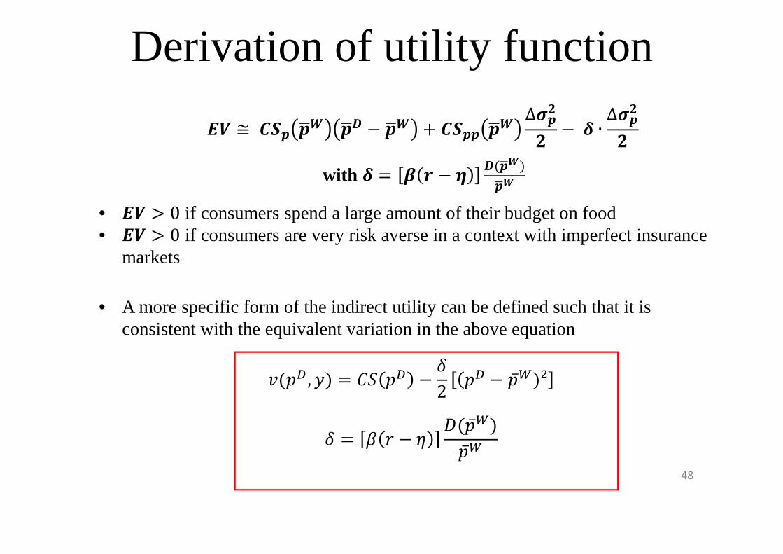
�" ≅ I� �%! �%� − �%! + I�� �%! ∆,�-- − J ∙ ∆,�-
-
with K = F() − G) 3(�%!)�%!
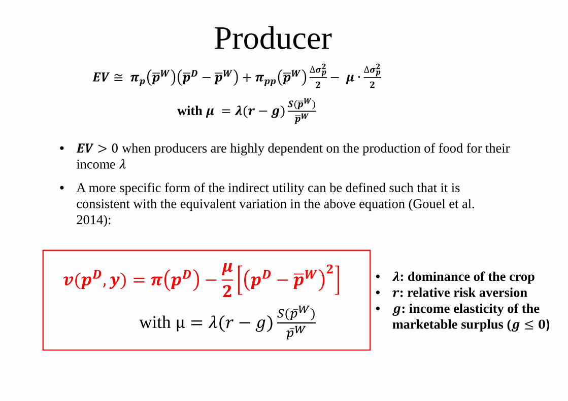
Producer�" ≅ I� �%! �%� − �%! + I�� �%! ∆,�-
- − J ∙ ∆,�--
with J = F() − G) 3(�%!)�%!
• A more specific form of the indirect utility can be defined such that it is consistent with the equivalent variation in the above equation (Gouel et al. 2014):
�(��, �) = I �� − J- �� − �%! -
• �" > 0 when producers are highly dependent on the production of food for their incomeL
with μ = L(: − N) O(C̅D)C̅D
• F: dominance of the crop • ): relative risk aversion• G: income elasticity of the
marketable surplus (G ≤ .)
The government
• Policy intervention to stabilize prices (with budgetary implications T):
� = �� − �> (< �� − @ �� )
• Government maximizes social welfare
PQRCS?@ �� − �
2 �� − �̅> � + � �� − T2 �� − �̅> �
+ �� − �> (< �� − @ �� )
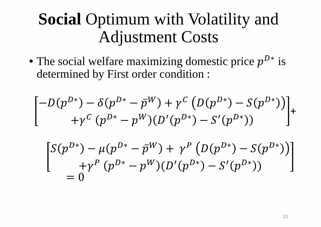
Social Optimum with Volatility and Adjustment Costs
• The social welfare maximizing domestic price ��∗ is determined by First order condition :
−< ��∗ − � ��∗ − �̅> + �� < ��∗ − @ ��∗
+�� ��∗ − �> <V ��∗ − @V ��∗ +
@ ��∗ − � ��∗ − �̅> +�� < ��∗ − @ ��∗
+�� ��∗ − �> (<V ��∗ − @V ��∗ )= 0
21
Social Optimum with Volatility
• First order condition can be written as:
• Case without volatility concerns:
��∗ − �> (<V ��∗ − @V ��∗ ) = � + � ��∗ − �̅>
��∗ − �> (<V ��∗ − @V ��∗ ) = 0
22
• First order condition can be written as:
or
Social Optimum with Volatility
��∗ = W�%! + 0 − W �!
withW = 4XJ4XJX3V�V ≥ . and . ≤ W ≤ 0
��∗ − �> = Y ��∗ − �̅>
with Y = ZX[�\OV = ]
]� ≤ 023
Social Optimum for different
24
• First order condition can be written as:
or
Social Optimum with Volatility
��∗ = ^�̅> + 1 − ^ �>
with^ = ZX[ZX[XOV�V ≥ 0 and 0 ≤ ^ ≤ 1
��∗ − �! = H ��∗ − �%!
with H = 4XJ�\3V = W
W0 ≤ .25
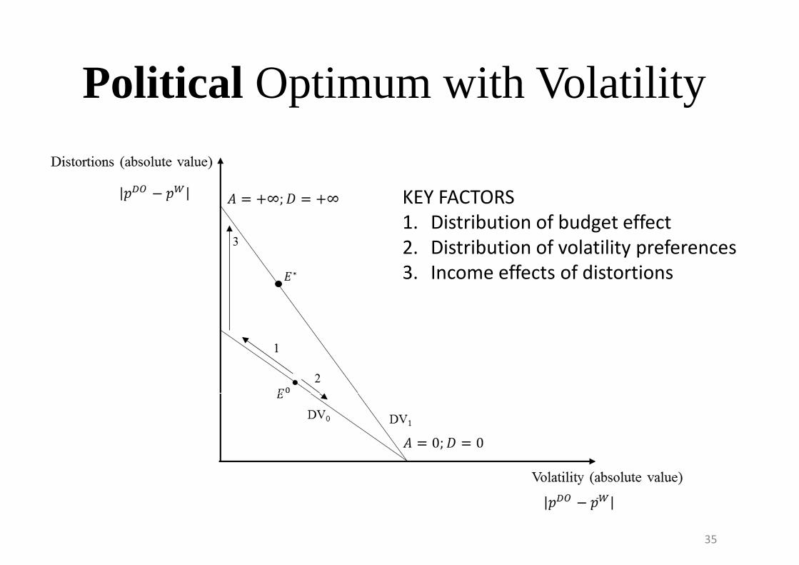
International price shocks and trade-off between distortions and volatility
26
Optimal combinations of observedvolatility and distortions for a givenprice shock
27
Empirical Evidence From developing countries
• Volatility (the coefficient of variation)
� = _�
• Distortions:
B = `1�
a
�bE��� − ��c
28
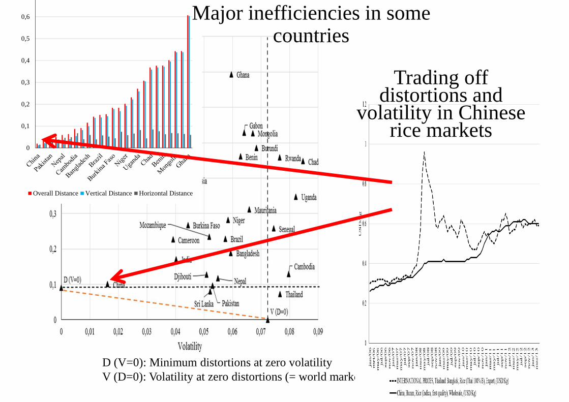
Distortions and volatility (2007-2013)
D (V=0): Minimum distortions at zero volatility V (D=0): Volatility at zero distortions (= world market price volatility)
29
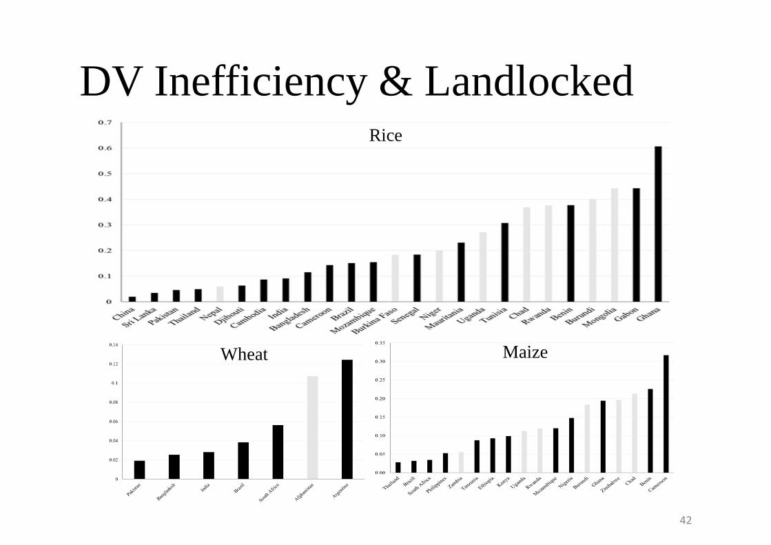
Rice Wheat
Maize
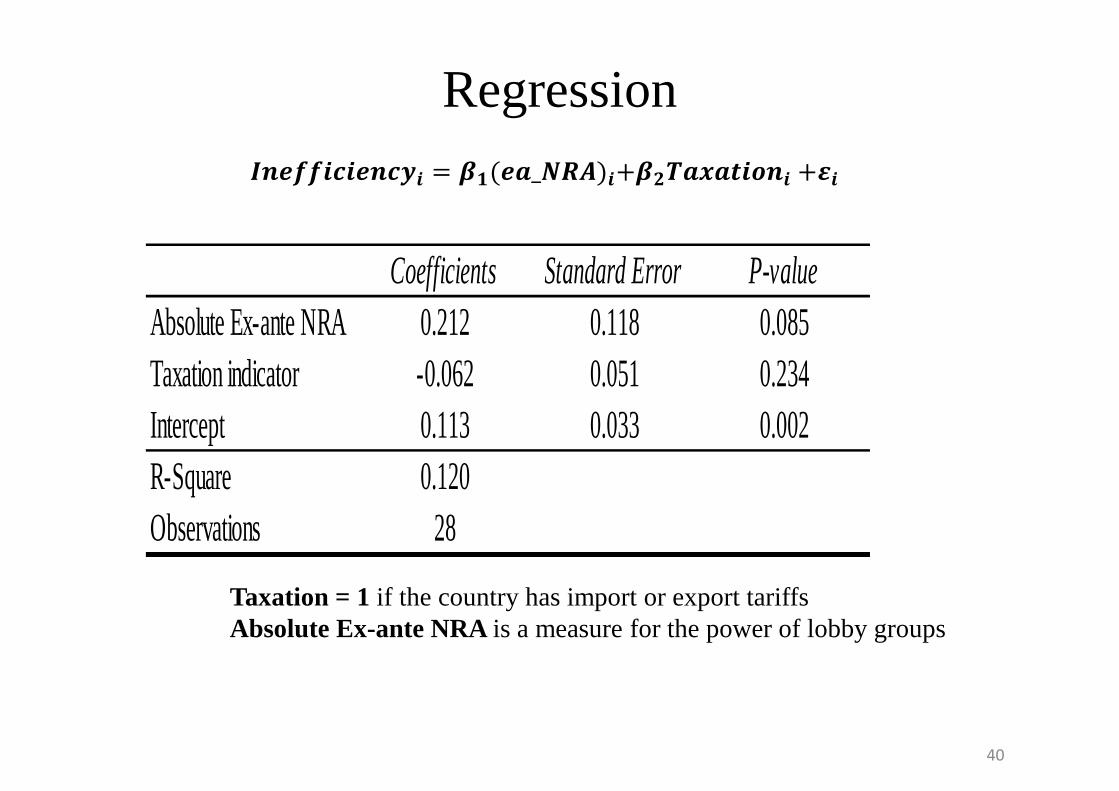
Empirical Evidence Measuring the inefficiency of the actual
policy
Dis
tort
ion
Volatility
Vertical Distance
Horizontal Distance
Overall Distance
Country A
Rice: DV frontier & inefficiency
D (V=0): Minimum distortions at zero volatility V (D=0): Volatility at zero distortions (= world market price volatility)
Taxation = 1 if the country has import or export tariffsAbsolute Ex-ante NRA is a measure for the power of lobby groupsLandlocked = 1 if country is landlockedNet-Import share = share of net imports in total trade
D (V=0): Minimum distortions at zero volatility V (D=0): Volatility at zero distortions (= world market price volatility)