64
TYÖPAPEREITA | WORKING PAPERS 309 Traditional convergence tests with Penn World Table 9.01 Sakari Lähdemäki*
| Date post: | 15-Apr-2017 |
| Category: |
Government & Nonprofit |
| Upload: | palkansaajien-tutkimuslaitos |
| View: | 109 times |
| Download: | 1 times |

TYÖPAPEREITA | WORKING PAPERS 309
Traditional convergence testswith Penn World Table 9.01
Sakari Lähdemäki*

Palkansaajien tutkimuslaitos
Labour Institute for Economic Research
Pitkänsillanranta 3 A
00530 Helsinki
www.labour.fi
Työpapereita | Working Papers 309
ISBN 978-952-209-154-3 (pdf)
ISSN 1795-1801 (pdf)
Helsinki 2016
I am grateful to Matti Virén, Eero Lehto and Tuomas Kosonen.
Futhermore I gratefully acknowledge the funding provided by Palkansaajasäätiö.
*[email protected], Labour Institute for Economic Research

Tiivistelmä
Konvergoituvatko eri maiden tuottavuustasot? Lahentyvatko kehittyvat maat kehittyneita
maita? Mitka maaryhmat konvergoituvat? Tassa tutkimuksessa pyritaan antamaan vas-
tauksia edelle esitettyihin kysymyksiin tarkastelemalla tyon tuottavuuden absoluuttista
konvergenssia ja sigma-konvergenssia Penn World Table 9.0 aineistolla. Absoluut-
tisella konvergenssilla tarkoitetaan yksinkertaistaen sita, etta mita alempi taso jollakin
taloudellisella mittarilla on suhteessa muihin maihin, sita suurempi on sen kasvuaste.
Sigma-konvergenssilla tarkoitetaan sita, etta jonkin taloudellisen mittarin eri maiden
tasojen hajonta pienenee jollakin aikavalilla. Tassa tutkimuksessa testataan konver-
goituvatko tiettyjen maaryhmien tuottavuustasot. Nama maaryhmat ovat seuraavat
kansainvaliset organisaatiot: OECD, EU ja APEC. Lisaksi testataan konvergoituvatko
seuraavien maanosien maat keskenaan: Afrikka, Aasia, Eurooppa ja Etela-Amerikka.
Tulosten mukaan konvergoitumista esiintyy seuraavissa maaryhmissa: OECD, EU, APEC,
Eurooppa ja Aasia. Tulosten mukaan Afrikassa ja Etela-Amerikassa konvergoituminen on
kuitenkin epavarmaa tai jopa olematonta.
JEL koodit: O40, O47, O52, O53, O54, O55
Avainsanat: absoluuttinen konvergenssi, beeta-konvergenssi, sigma-konvergenssi,
globalisaatio, tyon tuottavuus, OECD, EU, APEC, Eurooppa, Afrikka, Aasia, Etala-Amerikka
Abstract
Can we associate globalisation with converging productivity levels of different countries?
Are the developing countries catching up? Which speci ic country groups converge? This
paper provides answers to these questions by studying unconditional beta-convergence
and sigma-convergence of labour productivity with the Penn World Table 9.0 dataset.
Unconditional 𝛽-convergence exists if a smaller initial level of an economic measure is
related with a larger growth rate of this measure, whereas unconditional 𝜎-convergence
exists if the standard deviation of the levels of an economic measure decreases over
time. This paper tests the existence of convergence within speci ic country groups,
which are the international organisations OECD, EU and APEC, and the continents Africa,
Asia, Europe and South America. The tests support unconditional beta-convergence and
sigma-convergence in the country groups of OECD, EU, APEC, Europe and Asia, whereas
the convergence in Africa and South America is uncertain or non-existing.
JEL codes: O40, O47, O52, O53, O54, O55
Keywords: unconditional convergence, beta-convergence, sigma-convergence, glob-
alisation, labour productivity, OECD, EU, APEC, Europe, Africa, Asia, South America

Contents
1 Introduction 1
2 Data 4
3 Tests for unconditional convergence 6
3.1 Convergence concepts reviewed . . . . . . . . . . . . . . . . . . . . . . . . . . 6
3.2 𝛽-convergence . . . . . . . . . . . . . . . . . . . . . . . . . . . . . . . . . . . . 8
3.3 𝜎-convergence . . . . . . . . . . . . . . . . . . . . . . . . . . . . . . . . . . . . 9
4 Results 12
4.1 The world converging? . . . . . . . . . . . . . . . . . . . . . . . . . . . . . . . 12
4.2 OECD, EU and APEC . . . . . . . . . . . . . . . . . . . . . . . . . . . . . . . . . 15
4.3 Continent’s forming clubs? . . . . . . . . . . . . . . . . . . . . . . . . . . . . . 20
4.4 Panel Estimates for 𝛽-convergence . . . . . . . . . . . . . . . . . . . . . . . . 27
5 Conclusions 28
References 30
A Appendix 56
B Appendix 58

1 Introduction
A typical phrase concerning globalisation says that the world is getting smaller. By this
we mean that the accessibility of the world has improved vastly, for example, due to in-
formation technology and reduction in travel time. However it is questionable whether at
the same time there is an ongoing process which leads into smaller economic differences
between countries due to, for instance, international economic competition, capital move-
ment and diffusion of technology. That is, can we associate the ongoing globalisation with
the converging economic characteristics of different countries.
Why should we be interested? Firstly, simply because we are interested in how coun-
tries develop economically, for instance, whether or not developing countries catch up the
developed countries in living standards. Secondly, we are interested in whether there are
some country groups or international organisationswhere the convergence process differs
compared to the overall global economic convergence. Put differently, we are interested
in whether membership to, for instance, OECD signals growth behaviour that is different
compared to an outsider country.
Thirdly, and more importantly, the knowledge of economic convergence allows us to
optimize our policy making according to this information. For instance, it is valuable for
the developed European countries to know that the developing Eastern Europe converges
economically towards them. One reason for this is that in the long run productivity largely
determines wages and therefore the competitive advantage of the developing European
countries likely decreases. Furthermore, the catching up wage levels leads to new emerg-
ing markets within the developing European countries and so forth. Overall, when decid-
ing over long-term policy, such as investments, information over the development of the
companion countries is crucial.
Traditionally the convergence literature, which springs from the seminal paper by Bau-
mol (1986), tests the converging of economic performance indicators such as per capita
GDP, labour productivity, total factor productivity and wages. A vast part of this literature
concentrates on conditional convergence. These studies estimate a rate which measures
1

how fast economies return to their own steady states. However, when considering policy
making, the true value is in knowing which economies converge towards each other, that
is, unconditional convergence. Rodrik (2013) points out that convergence studies concen-
trate on conditional convergence since unconditional convergence is hard to ind at coun-
try level. In this paper I however show that unconditional convergence exists in speci ic
country groups. Furthermore I show that for some periods unconditional 𝛽-convergence
exits for all countries provided in the dataset.1
Therefore, the interest of this paper is in two concepts of convergence, unconditional
𝛽-convergence and 𝜎-convergence. Unconditional 𝛽-convergence exists when the rela-
tion between initial productivity levels and productivity growth rates is negative, that
is, the smaller the initial productivity level the faster the growth rate. Unconditional 𝜎-
convergence exists if the standard deviation of the productivity levels decreases over time.
Themain objective of this paper is to test the existence of these two convergence concepts,
that is, to study which country groups converge in productivity levels. In other words, I
simply study in which country groups unconditional convergence and 𝜎-convergence oc-
curs and in which it does it not.
This study contributes in three different ways as follows. Firstly, convergence stud-
ies typically test unconditional convergence with a speci ic narrow sample.2 Therefore,
due to different sample periods, different data sources, different country coverage and
different adopted tests the results are scattered and the comparability of these results is
questionable. This paper provides estimates from the harmonized Penn World Table 9.0
(PWT9.0) dataset for the periods 1960-2014, 1970-2014, ... ,2000-2014, and for all the
country groups that are traditionally tested. In this sense the unconditional convergence
rate estimates provided in this study are more comparable than the earlier estimates.
1The overall number of countries in the dataset is 182 from which 169 countries are covered with data
to calculate productivity for at least one of the periods considered. See appendix A.2See Dobson et al. (2006) for a table of traditional convergence studies.
2

Secondly, this study tests for 𝜎-convergence. As discussed later, a 𝜎-convergence test
is in a sense a more appropriate test for convergence compared to a 𝛽-convergence test.
Therefore another contribution of the present study is that it provides results from3differ-
ent𝜎-tests for the sameperiods and country groups that it provides the𝛽-estimates. These
three tests, provided by Carree and Klomp (1997) and Egger and Pfaffermayr (2009), test
whether the standard deviation of the productivity levels decreases over time within a
given country group.
Thirdly, this study testswhether three different GDPmeasures provided by the PWT9.0
dataset; living standards, productive capacity and national accounts GDP, lead to different
convergence estimates. For instance, countries might converge in living standards GDP
but not in productive capacity GDP. For more on the PWT9.0 dataset and different GDP
measures see section 2 and (Feenstra et al., 2015).
The test results indicate that convergence occurs in the country groups; OECD, EU and
APEC. Furthermore, also Europe and Asia as continents are converging indicating, for ex-
ample, that the former Eastern Bloc countries are catching up. However, the convergence
in terms of unconditional 𝛽-convergence and 𝜎-convergence is much more uncertain or
even non-existing in other continents considered, namely Africa and SouthAmerica. These
results reveal that indeed there are country groups that differ in the convergence process.
Furthermore, for some periods I ind support for 𝛽-convergence even in the World sam-
ple (all countries provided in the dataset). The 𝜎-convergence test however suggest that
the World has not been converging but rather diverging during the period 1960-2014. In-
terestingly I ind some evidence that after the year 2000 also the World has started to 𝜎-
converge.
The paper is structured as follows. In section 2 I give a short discussion concerning
the PWT9.0 dataset. A review of the different convergence concepts and a presentation
of the different convergence tests utilized in this paper are given in section 3. Results are
reported in section 4, whereas section 5 concludes.
3

2 Data
As Feenstra et al. (2015) note Penn World Tables have been standard data sources for
across country real GDP measures. Since the work of Summers and Heston (1988) the
dataset has advanced both in country coverage and in provided measures. Here my aim is
to test cross-country convergencewith the newly available PennWorld Table 9.0 (PWT9.0)
dataset.3
Themain interest in economic convergence is onwhether the real levels converge. The
focus is therefore on GDP measures based on prices which are constant across countries
and time. However construction of these real GDP series involves, for example, the estima-
tion of the purchasing power parities (PPP), which increases the risk of measurement er-
ror. For this reason in this study the real national accounts GDP serves as a steady baseline
while I study convergence also with the PPP ixed GDPmeasures. That is, I test labour pro-
ductivity (GDP per employment) convergence with the traditional national accounts GDP
based on national prices that are constant over time andwith two PPP ixed GDPmeasures
based on prices that are constant across countries and over time.4 All three measures are
from PWT9.0. The two PPP ixed GDP measures from PWT9.0 are the expenditure side
GDP which represents the living standards of a country and the output-side GDP which
represents the productive capacity of a country.
I present shortly the different measures of GDP. However for more on the data and the
3I irst did the same regressions and tests as here with the PWT8.1 dataset. There are three main dif-
ferences between PWT8.1 and PWT9.0. Firstly, the country coverage and the span are slightly improved in
PWT9.0. Secondly the new PPP benchmark (ICP2011) has been utilized to improve harmonization. Thirdly,
among ”normal” revisions to the national accounts data PWT9.0 better account for the more comprehen-
sive revisions set off by a growing number of countries that have shifted from the accounting rules of the
SNA1993 to the SNA2008. Overall the results from PWT9.0 compared to the results from PWT8.1 differ
mainly in favour of convergence.4To calculate labour productivity I use employment rather than hours worked since this increases the
number of observation notably.
4

differed GDP measures see Feenstra et al. (2015). The national accounts GDP is the real
GDP at constant national prices obtained from national accounts data and the base is in
2011 USA dollars. By the living standards GDP I refer to the expenditure side GDP mea-
sure in Feenstra et al. (2015), whereas by the productive capacity GDP I refer to the output
side GDP measure. Feenstra et al. (2015) convert GDP by inal goods PPP exchange rate
to produce the living standards GDP. Moreover they tread the trade balance as an income
transfer to the representative consumer and therefore it too is de lated by the inal goods
PPP exchange rate. The productive capacity GDP differs from the living standards GDP
since it is computed using PPPs speci ic to inal goods, imports and exports. Another fea-
ture of the PWT9.0 dataset is that it provides living standards GDP and productive capacity
GDP measures both in prices constant over country and in prices constant over time and
country. Basically these differ only in that for the measures based on prices constant both
in time and country the reference price vector is corrected from changing over time. For
more information how this exactly is done see Feenstra et al. (2015). Here I use the PPP
ixed GDP series that are based on prices that are constant over time and country as noted
above.
The PWT9.0 dataset spans the period 1950–2014. However most of the countries are
not covered this broadly. That is, for the year 1950 the dataset contains observations on
productivity for 32 countries, whereas for the year 1960 it contains already observations
for 82 countries. Then again for the founding OECD countries the full coverage starts from
1950 and for the EU-core countries from 1951. I start the analysis from the year 1960,
rather than 1950. The overall number of countries in the dataset is 182 from which 169
countries are covered with data to calculate productivity for at least one of the periods
considered. The country groups are listed in appendix A.
Often the interest in convergence papers is on a ixed time period, for example, Madsen
and Timol (2011) study unconditional labour productivity convergence in OECD countries
within the period 1870-2006. Here I however also test convergence within periods with
different initial years. I do this to give further evidence on whether the convergence rate
has changed during the 1960-2014 period. For example, it might be that for the irst 40
5

years of the studied period productivity levels converge and after that the convergence
shuts down. This case might result in non-rejection of the convergence hypothesis for the
whole periodwhen however sometime during the period converging has stopped. Accord-
ing to this reasoning I run the tests for the periods 1960-2014, 1970-2014, ... , 2000-2014.
Another important reason to consider different periods is that the available observations
increase the closer the initial year is to date.5
3 Tests for unconditional convergence
3.1 Convergence concepts reviewed
The convergence literature relates strongly with the growth literature. Traditionally the
convergence literature tests the economic convergence implied by the neoclassical growth
model by Solow (1956) and Swan (1956). Barro (2015) points out that the evolution of
growthmodels can bee seen simply as extending the neoclassical growthmodel, mainly by
endogenising the exogenous factors of the Solow-Swan framework. Rodrik (2013) states
that actually the lack of empirical support for unconditional convergence led the (exoge-
nous) growth theory into the endogenisation of the technological level and also into the
study of conditional convergence.
The traditional concepts of convergence are absolute, conditional and club conver-
gence.6 Assuming economies are structurally similar, characterized by the same steady
state. Then only the difference in the initial conditions of different economies affect con-
vergence. In this case convergence is called absolute or unconditional convergence. The
existence of unconditional convergence leads poor economies to catch up with the rich
5The obvious problem is that for some samples studied the number of available observations increases
from the period 1960-2014 to the period 2000-2014. This hampers the comparability of the periods with
different initial years. However I choose nevertheless to maximize the observations rather than to run the
regressions for the same observations for all considered periods for a given sample.6See also Quah (1993) for a slightly different de ining of convergence.
6

ones.
Barro (1991), after showing that in a large sample of countries unconditional conver-
gence is absent, controls for human capital and shows that there exists conditional conver-
gence. Barro and Sala-i-Martin (1992) and Mankiw et al. (1992) further study the concept
of conditional convergence. These papers state that countries converge towards their own
steady-states, and therefore it is necessary to control for the differences in steady-states
when studying convergence. Country speci ic steady-states howevermean that poor coun-
tries do not neccesarily converge towards the rich countries. Islam (1995) further studies
conditional convergence with a panel data approach.
Conditional convergence is compatible with differences among economies, in which
case these differences spring from the structural differences of these economies. How-
ever systematic differences (non-convexities), for example, different available technology
at different levels of economic development, might result in stages of growth or in other
words multiple steady-state equilibria. Then clubs of converging countries can emerge as
Durlauf and Johnson (1995) and Desdoigts (1999) propose, see also Baumol (1986).
When considering the three convergence concepts discussed shortly above we speaks
of 𝛽-convergence. The interest is then mainly on whether the initial productivity level is
negatively related to the growth rates of productivity in an unconditional, a conditional or
a multiple regime (club convergence) setting.
Additionally there is the concepts of 𝜎-convergence. Baumol (1986) in his article notes
shortly that the dispersion of the cross-sectional productivity has decreased in the stud-
ied sample. Friedman (1992) argues that indeed this is a more relevant concept of con-
vergence. This is because even if 𝛽-convergence exists it might be that the dispersion of
the productivity levels across countries does not decrease over time. Indeed Friedman
(1992) and Quah (1993) argue that 𝛽-convergence regression is tainted by regression fal-
lacy, namely regression towards the mean. Friedman (1992) further argues that due to
this fallacy a test of decreasing dispersion of the productivity levels over time is a more
appropriate test for convergence. Lichtenberg (1994) is the irst to propose a statistical
test for 𝜎-convergence.
7

Sala-i-Martin (1996) argues that both 𝛽-convergence and 𝜎-convergence are inter-
esting and give insight to different questions. That is, 𝛽-convergence studies the mo-
bility within the distribution, whereas 𝜎-convergence studies the evolution of the dis-
tribution. Sala-i-Martin (1996) also shows the relationship between 𝜎-convergence and
𝛽-convergence, that is, 𝛽-convergence is a necessary but not a suf icient condition of 𝜎-
convergence, see also Lichtenberg (1994). In the next two sections I shortly present the 𝛽-
and 𝜎-tests I utilize in this paper.
3.2 𝛽-convergence
To test the existence of unconditional convergence in the productivity levels I adopt the
so called 𝛽-convergence test. For founding studies of 𝛽-convergence, see Baumol (1986)
and Barro and Sala-i-Martin (1992). For amore resent study see, for instance, Madsen and
Timol (2011). The test for unconditional 𝛽-convergence is a simple regression as follows:
Δ ln(𝑌𝐿 ) = 𝛼 + 𝛽 ln(𝑌𝐿 ) + 𝜖 (1)
Or
ln(𝑌𝐿 ) = 𝛼 + 𝜋 ln(𝑌𝐿 ) + 𝜖 , 𝑤ℎ𝑒𝑟𝑒 𝜋 = (1 + 𝛽 ) (2)
Where ln(𝑌/𝐿) is the initial log productivity level, ln(𝑌/𝐿) is the log productivity level
in the last period and Δ ln(𝑌/𝐿) is the (average) growth rate in between the initial year
and the last year, 𝜖 is a stochastic error term. The null hypothesis of no 𝛽-convergence is
rejected if the coef icient 𝛽 is negative and statistically signi icant.
Furthermore Barro and Sala-i-Martin (1992) and Sala-i-Martin (1996) estimate a non-
linear 𝛽-convergence regression to produce estimates that are directly comparable across
samples with different initial years. The regression is as follows:
1𝑇Δ ln(
𝑌𝐿 ) = 𝛼 + (1 − 𝑒
𝑇 ) ln(𝑌𝐿 ) + 𝜖 (3)
The reasoning behind the non-linear version, as Barro and Sala-i-Martin (1992) and Sala-i-
Martin (1996) state, is as follows. When convergence exists initially countries grow faster.
The average growth rate of a long time period is then surely a combination of the more
8
fast growth in the earlier periods and also the slower growth in the later periods. In other
words, as T gets larger the effect of the initial position on the average growth rate becomes
smaller.
In Baumol (1986) the dependent variable in regressing (1) is the growth rate, whereas
for example in Madsen and Timol (2011) the dependent variable is the average growth
rate. In this paper the dependent variable in regression (1) is the average growth rate
rather than the growth rate. However I prefer regression (3) since the estimation allows
the direct comparison of the convergence rate estimates for samples with different time
spans.
While the main interest is on regression (3), for robustness, I also run regression (1)
transformed into a panel regression where the time dimension is formed from three- ive-
and ten-year intervals of the data. According to my knowledge, Islam (1995) is the irst to
study conditional convergence in a panel data setting. I do not add the ixed effects into
the panel regression (1) since I study unconditional convergence. However I add time ef-
fects to adjust for over time changingworld (club) average growth rates. For recent papers
studing unconditional convergence in a panel data setting see Madsen and Timol (2011)
and Rodrik (2013).
A short comment on interpreting the results, Madsen and Timol (2011) note that they
interpret their results on a basis of a one-sided critical value since they test rather 𝛽 < 0
than is 𝛽 signi icantly different from zero. I agree that in their paper the one-sided test is
justi iable since the focus is on OECD countries which are often found to converge. How-
ever in this paper interpretation is throughout done based on the two-sided critical values.
That is I make no prior assumptions of the sign of 𝛽 or of convergence.
3.3 𝜎-convergence
A 𝜎-convergence test is a test whether the standard deviation of the productivity levels de-
creases over time. Here I shortly present a 𝜎-convergence tests proposed by Lichtenberg
(1994), an adjusted version of Lichtenberg’s (1994) and an alternative likelihood-ratio test
both proposed by Carree and Klomp (1997) and furthermore an alternativeWald test pro-
9

posed by Egger and Pfaffermayr (2009). The test statistic in Lichtenberg (1994) is:
𝑇 =���� (4)
Where �� denotes the cross-country variance of productivity in the initial period and
�� the variance in the last period. According to Lichtenberg (1994) the test statistic is
asymptotically 𝐹 distributed with𝑁−2 degrees of freedom in both the nominator and the
denominator.
Carree and Klomp (1997) argue that actually the test in Lichtenberg (1994) is 𝐹 dis-
tributed with𝑁−1 degrees of freedom instead of𝑁−2. Moreover they show that �� and
�� are not independently distributed when 𝜋 ≠ 0, implying that Lichtenberg’s (1994) test
is not 𝐹 distributed and is biased towards inding no convergence, that is, a type II error.
Therefore Carree and Klomp (1997) propose an adjusted version of the ratio of variances
test which is standard normal distributed. They also derive an alternative likelihood-ratio
based test. In their simulations they ind that their likelihood-ratio test is more close to its
asymptotic distribution even with small values of 𝑁. The test statistics are as follows:
𝑇 =√𝑁(�� /�� − 1)
2√1 − ��(5)
𝑇 = (𝑁 − 2.5) ln 1 + 14(�� − �� )�� �� − �� ,
(6)
Where �� denotes the cross-country variance of productivity in the initial period, ��
the variance in the last period and �� is the coef icient estimate of regression (2). The term
�� , is the covariance of productivities in the initial and last period. The test 𝑇 is asymp-
totically 𝜒 distributed with 1 degree of freedom. Carree and Klomp (1997) point out that
when considering the power of the tests, that is, the probability to correctly reject the null,
the likelihood-ratio test and the adjusted ratio of variances test outperforms the test Licht-
enberg (1994) proposes.
A more recent paper by Egger and Pfaffermayr (2009) propose a Wald test for test-
ing 𝜎-convergence. They note that when considering unconditional convergence their test
10

performs equally well in their simulations as the likelihood test Carree and Klomp (1997)
propose. However when considering conditional 𝜎-convergence, the test has some advan-
tages over the likelihood-ratio test. Here I utilize the test to increase the robustness of the
analysis. The test statistic for unconditional 𝜎-convergence is:
𝑇 = (𝑁 − 2.5)4
�� − 1 +
�� (7)
Where �� denotes the cross-country variance of productivity in the initial period, the term
�� is the estimated variance of the error term in regression (2) and �� is the coef icient
estimate of regression (2). In both tests 𝑇 and 𝑇 I use (𝑁−2.5) rather than𝑁 to improve
the 𝜒 approximation in small samples7.
As pointed out Lichtenberg’s (1994) test 𝑇 is biased towards inding no convergence
and it’s adjusted version 𝑇 performsworse than the likelihood-ratio test in small samples.
However the hypothesis that the variance of productivities is decreasing is more practical
in situations where the dispersion is increasing compared to 𝑇 and 𝑇 which𝐻 hypothe-
ses are �� = �� and 𝜋 = �� respectively. The tests 𝑇 and 𝑇 therefore test whether the
initial value and end value are the same. The fact that they are not the samewith increasing
dispersion leads to rejection of the null when there is no 𝜎-convergence but 𝜎-divergence.
Another problem with 𝑇 arises when|𝜋| > 1 since then 𝑇 cannot be determined. As in
Carree and Klomp (1997) I interpret these cases as no convergence.
I prefer 𝑇 over the other test’s. However the tests 𝑇 and 𝑇 provide further evidence
especially when the sample size is small. Furthermore I represent a igure depicting the
development of the productivity level standard deviation for most of the studied samples.
This aids to interpret the 𝜎-tests especially in cases where the dispersion is in fact increas-
ing.
7Conserning the multiplying factor of the approximation Carree and Klomp (1997) and Egger and
Pfaffermayr (2009) both refer to an older edition of Morrison (2005). However atleast in this newer edition
Morrison (2005) refers to Bartlett (1954).
11

4 Results
4.1 The world converging?
The results from the NLS-regression (3) for the sample of all countries are shown in table
6. The columns of table 6 contain the 𝛽-estimates for the different periods, whereas the
different measures of GDP for a speci ic sample are reported row-wise. The standard er-
rors of the coef icients are heteroscedasticity robust (White, 1980), whereas the 𝑝-values
are from the 𝑇 distribution with 𝑁 − 2 degrees of freedom. For brevity I report only the
signi icances of the estimates in table 6. The number of observations differs for different
initial years as more observations are available the nearer the initial years is to date.
The coef icient estimates for the sample of all countries are all negative and from on
the initial year 1970 signi icant at the 0.1 signi icance level, moreover except for one case
all the estimates are signi icant at the 0.05 signi icance level. For the period 1960-2014
only the estimate for national accounts GDP is signi icant at the 0.1 signi icance level and
furthermore all the estimates for this period are close to zero. For the period 2000-2014
the estimates are notably smaller indicating that the𝛽-convergence has been ongoingwith
a larger rate compared to the other periods. Overall the different GDP measures result in
seemingly similar estimates of the𝛽-coef icients the only exception being that the national
accounts GDP estimates are more often signi icant.
The results in table 6 differ from the earlier studies by Barro (1991) and Barro and
Sala-i-Martin (1992). For example Barro and Sala-i-Martin (1992) ind a positive 𝛽 for
the period 1960-1985 in a rich cross-country setting consisting of 98 countries from the
Summers and Heston (1988) dataset. Moreover Rodrik (2013) claims that actually uncon-
ditional convergence can only be found among the states/regions of an uni ied economy
such as United States or the country group OECD. The results in table 6 however indicate
that from on the initial year 1970 the world has been 𝛽-converging.
The difference between the earlier results and the results heremight spring from three
different sources. Firstly, the larger sample size might affect the results, indicating that
12

the sample selection bias contaminates the earlier results. Secondly, the difference might
result from the different span of the sample indicating that the convergence process is
stronger in the later years of the whole period 1960-2014. The fact that the estimates are
close to zero for the period 1960-2014 supports this conclusion. Thirdly, the improve-
ments in the quality of the dataset most likely affects the results.8
The studies by Quah (1993, 1996) indicate that there is no unconditional convergence
to be found in a rich cross-country setting further stating that actually rich countries get
richer and poor countries poorer. Therefore, to further study convergence in the universal
scope I run the 𝜎-tests for the World sample. Overall the tests for 𝜎-convergence support
the claims in Quah (1993, 1996) that actually rich countries get richer and poor countries
poorer. Figure 1 depicts the increasing dispersion of the productivity levels in the period
1960-2014. The 𝜎-tests are reported in table 1 where I report the test statistics and the
associated 𝑝-values in parenthesis for the tests 𝑇 , 𝑇 , 𝑇 . A − sign marks the cases where
𝑇 is not determined. The number of observations differs for different initial years asmore
observations are available the nearer the initial years is to date.
[Figure 1 here.]
Figure 1 shows clear increasing in the dispersion of productivity from 1960 to 2014.
Overall the evolution of the productivity dispersion is quite similar for all the GDP mea-
sures. The fact that more observations were available in the later years might affect the
standard deviation increasingly as the latest countries added to the dataset are likely eco-
nomically more far behind compared to the countries providing data early on. To avoid
this shortcoming I depict two different lines. The red line is the standard deviation of only
8It is somewhat interesting to notice that the results from the PWT8.1 dataset differs from the results
shown here while the sample size in PWT9.0 is only slightly larger. Moreover, PWT9.0 produces larger (in
absolute terms) -regression estimates and improves the signi icances of these estimates probably since
the better harmonization of the data. However in both datasets the -convergence in the period 2000-2014
(2000-2011 for PWT8.1) is evident.
13

the countries covered for all years,𝑁 = 82, whereas the blue line is the standard deviation
of all countries provided in a particular year, that is, 𝑁 increases along the x-axis.
Despite the clear overall increase of productivity dispersion an interesting observation
is that after the year 2000 it seems that the dispersion starts to decrease (at least when
considering the 82 countries covered for all years). This result emerges also from table 1.
Fromon the initial year 2000 the tests for the productive capacity GDP and living standards
GDP come close to the rejection of the null at the 0.05 signi icance level. The test for the
national accounts GDP rejects the null in favour of 𝜎-convergence.
[Table 1 here.]
The results of 𝛽-convergence tests are in line with the 𝜎-tests since both suggest con-
vergence from on the initial years 2000. Whether there actually is a turning point towards
the convergence of the world productivities somewhere in the beginning of the 21st cen-
tury remains to be seen. However the claim by Rodrik (2013) that actually unconditional
convergence can only be found among the states/regions of an uni ied economy such as
United States or the country group OECD, does not seem to hold, at least not with the data
provided by PWT9.0. That is, for the sample of all provided countries 𝛽-convergence ex-
its from on the initial year 1970 and the convergence rate is even larger from on the year
2000. Despite the existing 𝛽-convergence from on 1970 the 𝜎-convergence seems to start
only after the year 2000.
To test whether some regions or clubs convergence I next divide the dataset into coun-
try groups, or in other words into subsets of the whole dataset, as is common in the club
convergence literature. See, for instance, Durlauf and Johnson (1995). I form subsam-
ples (clubs) directly from continents and international organisations, namely OECD, EU
and APEC. For the content of each country group see appendix A. The further results are
in some favour of the concept of club-convergence studied earlier by Durlauf and Johnson
(1995), Quah (1997), Desdoigts (1999) andmore recently, for example, Bernardini Papalia
and Bertarelli (2013).
14

4.2 OECD, EU and APEC
I start this sectionwith the results for OECD countries. As is common in the literature I ind
that OECD countries converge. For instance Madsen and Timol (2011) inds evidence on
converging manufacturing labour productivity among the OECD countries for the period
1870-2006. Indeed the 𝛽-regressions reported in table 6 for the founding OECD countries
produce negative estimates which are all signi icant at the 0.1 signi icance level for all ini-
tial years and GDP measures. One interesting detail is that the speed of convergence is
higher for the initial years starting from 2000 than for the earlier initial years.
The green line in igure 2 depicts the productivity dispersion for the OECD founders,
𝑁 = 20. There has been clear 𝜎-convergence from on the initial year 1960. However from
the initial year 1990 onwards the 𝜎-tests, which are not reported (available on request),
result often in p-values larger than 0.05. Indeed igure 2 supports the test results with the
standard deviation stabilizing somewhere around 0.25 after the year 1990.
[Figure 2 here.]
The founders of OECD have been converging within the period 1960-2014. However
the club has grown since the beginning of its formation in 1961 from its founding 20 to
its present 34 members. The results from 𝛽-regressions with all current OECD member
countries included are reported in table 6. Here I include all countries available to the
regression, that is, also the countries that during an initial year were not yet members but
countries to becomemembers. It is questionable howmuch the characteristics of the club
affect the convergence of its members. More likely there are countries that possess some
characteristics and are therefore desired as club members.
The results from the𝛽-regressions for the founders of OECD and for all OECD countries
are seemingly similar. This is expected since the founders still account for most of the
observations. However, when adding the other OECD countries to the sample of OECD
founders all the estimates are signi icant at the 0.01 signi icance level and the absolute
values of the estimates are larger compared to the sample of the founders. This strengthens
the conclusion that OECD countries are converging in the productivity levels. The 𝜎-tests
15

reported in table 2 and the depicted dispersion in igure 2 further con irms that also the
productivity dispersion is decreasing within the sample of all OECD countries.
[Table 2 here.]
In igure 2 there are two lines in addition to the above mentioned green line. The red
line is the standard deviation of only those OECD countries that are covered for all years,
𝑁 = 28, whereas the blue line is the standard deviation of all OECD countries provided
in a particular year. The two countries added in 1970 increase the standard deviation re-
markably compared to the standard deviation shown by the red line, however the overall
decreasing of productivity dispersion is evident. The 𝜎-tests in table 2 reject the null more
often than with the sample of the OECD founders, actually in all cases at the 0.05 signi i-
cance level, indicating that the 𝜎-convergence is more eminent when considering all OECD
countries.
[Figure 3 here.]
Overall the results support the earlier indings that indeed OECD countries are con-
verging. Moreover the conclusion holds whether considering national accounts GDP or
the more sophisticated measures of GDP. I ind that among the founding OECD countries
the dispersion of productivity levels has clearly decreased compared to the year 1960how-
ever after the year 1990 the decreasing is uncertain. With the sample of all OECD countries
𝜎-convergence is evident in all period considered.
I further study convergence in EU. Both organisations EU andOECD advocate economic
and political integration within the member countries. OECD evolved from the former
Organisation for European Economic Co-operation (OEEC) which was initially set up to
administer Marshall Plan the recovery program for Europe after the Second World War.
OECD had also non-European founders, namely USA and Canada, and has enlarged inter-
nationally. EU evolved from European Atomic Energy Community (EURATOM), European
Coal and Steel Community (ECSC) and European Economic Community (EEC) and has en-
larged only in Europe. Since 21 out of the total 28 countries in EU are also members in
16

OECD (See appendix A), one would expect that convergence is present also in EU. Indeed
this is what I ind.
[Table 3 here.]
The results from the NLS-regression (3) for core EU countries and all EU countries are
reported in table 6. The 𝛽-estimates for core EU countries are signi icant at the 0.01 level
with the exception that the estimates for the initial years 1990 and 2000 for national ac-
counts GDP are not signi icant. Adding the additional EU countries to the sample of core EU
countries con irms the inding that productivity levels 𝛽-converge in EU. Compared to the
results for the core EU countries the results are even more explicit. All the estimates are
signi icant and they are more often larger than smaller in absolute terms compared to the
core EU estimates. One interesting observation is that compared to the sample of OECD
countries the rate of convergence within the period 2000-2014 is seemingly stronger in
the sample of EU countries.
I report the 𝜎-tests for all EU countries in table 3. According to the tests there is def-
initely 𝜎-convergence in EU. All tests 𝑇 , 𝑇 and 𝑇 reject the null at the 0.05 signi icance
level. This result is con irmed in igure 3 which depicts the evolution of the productivity
dispersion for all EU countries. The red line in igure 3 is the standard deviation of only
the countries covered for all years,𝑁 = 18, whereas the blue line is the standard deviation
of all countries provided in a particular year. The observation is evident. The dispersion
has decreased among the EU countries from 1960 to 2014.
To save space I don’t report the𝜎-tests for the sample of core EU countries (available on
request). However I note that the results are similar to the results for the OECD founders.
That is, sometime around the 1970s the productivity dispersion saturated somewhere
around 0.2 and there by stopped decreasing. This result emerges also from igure 3 where
the green line represents the productivity dispersion for the core EU countries,𝑁 = 15.
[Figure 4 here.]
The literature shows somewhat less attention on the development of the Asia-Paci ic
17
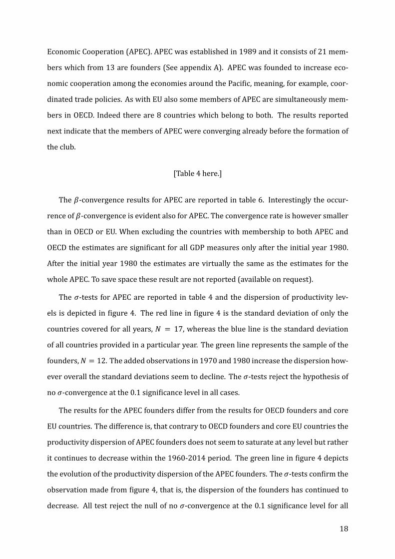
Economic Cooperation (APEC). APEC was established in 1989 and it consists of 21mem-
bers which from 13 are founders (See appendix A). APEC was founded to increase eco-
nomic cooperation among the economies around the Paci ic, meaning, for example, coor-
dinated trade policies. As with EU also some members of APEC are simultaneously mem-
bers in OECD. Indeed there are 8 countries which belong to both. The results reported
next indicate that the members of APEC were converging already before the formation of
the club.
[Table 4 here.]
The 𝛽-convergence results for APEC are reported in table 6. Interestingly the occur-
rence of 𝛽-convergence is evident also for APEC. The convergence rate is however smaller
than in OECD or EU. When excluding the countries with membership to both APEC and
OECD the estimates are signi icant for all GDP measures only after the initial year 1980.
After the initial year 1980 the estimates are virtually the same as the estimates for the
whole APEC. To save space these result are not reported (available on request).
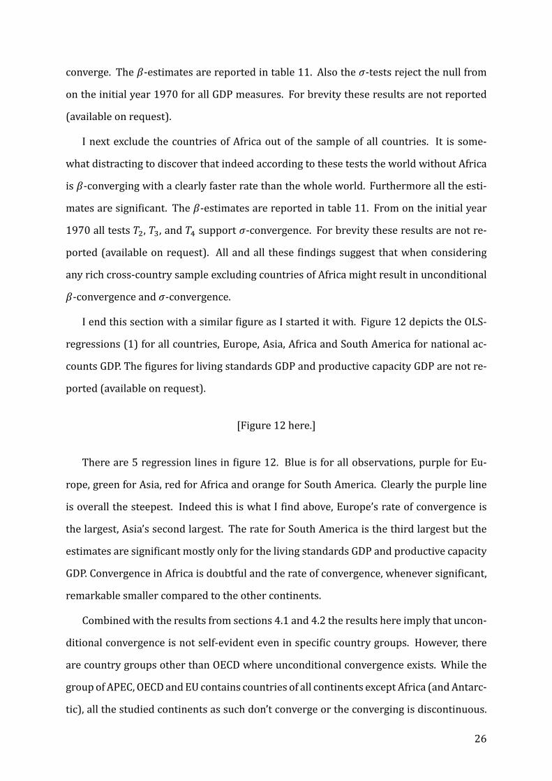
The 𝜎-tests for APEC are reported in table 4 and the dispersion of productivity lev-
els is depicted in igure 4. The red line in igure 4 is the standard deviation of only the
countries covered for all years, 𝑁 = 17, whereas the blue line is the standard deviation
of all countries provided in a particular year. The green line represents the sample of the
founders,𝑁 = 12. The added observations in 1970 and 1980 increase the dispersion how-
ever overall the standard deviations seem to decline. The 𝜎-tests reject the hypothesis of
no 𝜎-convergence at the 0.1 signi icance level in all cases.
The results for the APEC founders differ from the results for OECD founders and core
EU countries. The difference is, that contrary to OECD founders and core EU countries the
productivity dispersion of APEC founders does not seem to saturate at any level but rather
it continues to decrease within the 1960-2014 period. The green line in igure 4 depicts
the evolution of the productivity dispersion of the APEC founders. The 𝜎-tests con irm the
observation made from igure 4, that is, the dispersion of the founders has continued to
decrease. All test reject the null of no 𝜎-convergence at the 0.1 signi icance level for all
18

periods and all GDP measures. For brevity these results are not reported (available on
request). The dispersion is also remarkably larger compared to OECD founders and core
EU. The values of the estimated 𝛽-coef icients for the APEC founders compared to the 𝛽-
coef icients for all APEC countries are virtually the same.
[Figure 5 here.]
In this section there is yet onematter of interest. Since countries in OECD, EU andAPEC
all converge within the respective club, it is most expected that when combined together
as a single group, convergence occurs also within this new group. Indeed this is what I
ind. The results for this combined sample are reported in table 6. All the 𝛽-estimates
are negative and signi icant. The 𝜎-tests 𝑇 , 𝑇 and 𝑇 reported in table 5 all reject the
hypothesis of no𝜎-convergence. Both lines in igure 5 decline steeply for all GDPmeasures.
The red line is the standard deviation of only the countries covered for all years, 𝑁 = 40,
and the blue line is the standard deviation of all countries provided in a particular year.
[Table 5 here.]
All and all both partly overlapping club’s OECD and EU have been converging in terms
of both 𝛽- and 𝜎-convergence. Moreover adding the later-joined-members to the sam-
ple of founders rather strengthens the rate of convergence implying that the later-joined-
members are caching up. Therefore, the results support the earlier indings of the conver-
gence literature, that is, convergence occurs in OECD and EU. I also ind that APEC is 𝛽-
and 𝜎-converging however the convergence rate is smaller compared to EU and OECD and
the 𝜎-convergence is slightly more uncertain. When combining the countries of OECD, EU
and APEC into one sample, according to the considered tests, both 𝛽- and 𝜎-convergence
are indisputable.
[Table 6 here.]
19

4.3 Continent’s forming clubs?
I start this section by noting that the rate of convergence for the whole sample is remark-
ably smaller compared to the group of APEC, EU and OECD countries. In the spirit of Bau-
mol (1986) I depict the OLS-regressions (1) for the whole world and for a club consisting
the members of OECD, EU and APEC in igure 6 for the national accounts GDP. The ig-
ures for living standards GDP and productive capacity GDP are not reported (available on
request) however overall they are seemingly similar with igure 6.
[Figure 6 here.]
The blue dots in igure 6 are the observations of the club, whereas the red dots and the
blue dots together form the observations of the world. The red regression line is from the
sample of all dots, whereas the blue regression line is from the club sample. As evident
from sections 4.1 and 4.2 the blue line has a clearly larger slope in absolute terms than the
red line. Moreover, as the initial year grows the blue dots seem to concentratemore closely
with each other contrary to all the dots.
According to the test results in sections 4.1 and 4.2the international organisations
APEC, EU and OECD converge faster than the sample of all countries raises the question
whether there are other country groups which also have a converge rate that is faster than
the ”world’s normal” rate. Furthermore, are there some country groups which are respon-
sible for the lower ”world’s normal” convergence rate. In this section I provide some in-
sight over these questions.
The literature gives no unambiguous practice to de ine clubs. Durlauf and Johnson
(1995) form clubs with reference to countries stage of development, whereas Desdoigts
(1999) propose a geographical structure. A more recent paper by Bernardini Papalia and
Bertarelli (2013) utilize a mapping model to detect clubs from TFP-levels. Furthermore
theynote that the clubs they formare in linewithDurlauf and Johnson (1995) and they ind
that each group𝛽-convergeswith a unique rate in a conditionalmultiple regime panel data
setting. The paper however does not test unconditional convergence or 𝜎-convergence.
Anyhowhere I simply formgroups straight from the continents, that is, the clubs areAfrica,
20
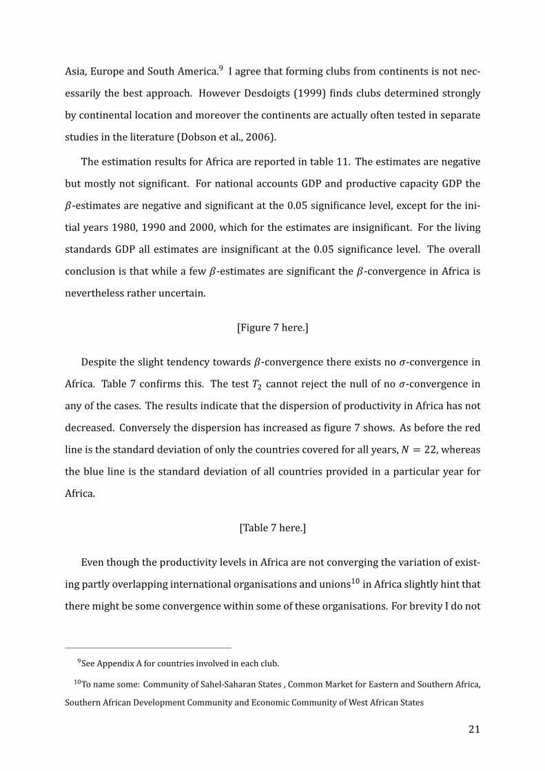
Asia, Europe and South America.9 I agree that forming clubs from continents is not nec-
essarily the best approach. However Desdoigts (1999) inds clubs determined strongly
by continental location and moreover the continents are actually often tested in separate
studies in the literature (Dobson et al., 2006).
The estimation results for Africa are reported in table 11. The estimates are negative
but mostly not signi icant. For national accounts GDP and productive capacity GDP the
𝛽-estimates are negative and signi icant at the 0.05 signi icance level, except for the ini-
tial years 1980, 1990 and 2000, which for the estimates are insigni icant. For the living
standards GDP all estimates are insigni icant at the 0.05 signi icance level. The overall
conclusion is that while a few 𝛽-estimates are signi icant the 𝛽-convergence in Africa is
nevertheless rather uncertain.
[Figure 7 here.]
Despite the slight tendency towards 𝛽-convergence there exists no 𝜎-convergence in
Africa. Table 7 con irms this. The test 𝑇 cannot reject the null of no 𝜎-convergence in
any of the cases. The results indicate that the dispersion of productivity in Africa has not
decreased. Conversely the dispersion has increased as igure 7 shows. As before the red
line is the standard deviation of only the countries covered for all years, 𝑁 = 22, whereas
the blue line is the standard deviation of all countries provided in a particular year for
Africa.
[Table 7 here.]
Even though the productivity levels in Africa are not converging the variation of exist-
ing partly overlapping international organisations and unions10 in Africa slightly hint that
there might be some convergence within some of these organisations. For brevity I do not
9See Appendix A for countries involved in each club.10To name some: Community of Sahel-Saharan States , Common Market for Eastern and Southern Africa,
Southern African Development Community and Economic Community of West African States
21

test the converging of these organisations in this study. The sample of Africa is however
divided into North-West-South (𝑁 = 26) countries and East-Central countries (𝑁 = 24).
These groups donot converge. For both theNorth-West-South sample and the East-Central
sample some of the 𝛽-estimates turn out signi icant and negative. Nevertheless for both
samples the 𝜎-tests do not reject the hypotheses of no sigma-convergence in any period,
implying that splitting Africa roughly into two groups consisting about the samenumber of
countries does not alter the result that Africa is not 𝜎-converging. For brevity these results
are not reported (available on request).
The results for Asia are reported in table 11. Except for one case the estimates for all
the GDP measures are negative and signi icant at the 0.05 signi icance level (all are signif-
icant at the 0.1 level). The overall conclusions is that Asia is 𝛽-converging in all the GDP
measures. Moreover, the rate of convergence increases as the initial year gets closer to
date.
The productivity dispersion of Asia is depicted in igure 8. Again the red line is the
standard deviation of only the countries covered for all years, 𝑁 = 19, whereas the blue
line is the standard deviation of all countries provided in the particular year. The irst
notice is that the increase of 𝑁 = 19 to 𝑁 = 29 in the year 1970 increased the dispersion
remarkably. From the beginning of the 70s there however seems to be some decreasing in
the blue line, whereas the red line shows some increasing of the dispersion except for the
national accounts GDP.
[Figure 8 here.]
The 𝜎-test results in table 8 con irm the observations made from igure 8. All the GDP
measures are 𝜎-converging from on the initial year 1970. However, for the period 1960-
2014 none of the tests reject the null. Clearly the additional observations from on 1970
affects the test results in favour of 𝜎-convergence.
[Table 8 here.]
Southeast Asia can be seen as a separate club (Desdoigts, 1999). This area consists of
22

observations from 10 countries which are also the members of the Association of South-
east Asian Nations (ASEAN). I test whether this group of countries is converging. The esti-
mates for the initial years 1960 and 1970 are all insigni icant and often close to zero. From
on the initial year 1980 however the 𝛽-coef icients are negative and signi icant for all the
GDP measures. Indicating that the club 𝛽-converges from on the initial year 1980. The
𝛽-estimates are reported in table 11.
The𝜎-tests for Southeast Asia show thatwithin the period 1980-2014 the dispersion of
productivity levels of all GDPmeasures consideredhavedecreasedhowever thedecreasing
has stopped from on the initial year 1990. Interestingly this is somewhat the story also for
the sample of all Asian countries as igure 8 depicts. For brevity estimates for the ASEAN
countries are not reported (available on request).
The results for Europe are reported in table 11. The results are clear. The estimates
are negative and signi icant at the 0.01 signi icance level for all GDP measures and all ini-
tial years. Moreover the rate of convergence is faster for the later initial years, which is
partly due to the increase in observations. This result suggests that the countries which
are covered only for the later years in the dataset are catching up. Most of these countries
belonged to the so called Eastern Bloc. The results for Europe were obviously predictable
from the results reported in section 4.2. After all from Europe’s 40 countries 28 are mem-
bers of EU.
[Figure 9 here.]
The results for Europe’s 𝜎-tests in table 9 indicate clear 𝜎-convergence as expected.
This is indeed the result taking shape in igure 9. The red line indicates the standard de-
viation of only the countries covered for all years, 𝑁 = 21, whereas the blue line is the
standard deviation of all countries provided in a particular year. The blue line increases
steeply between the years 1969-1970 and the years 1989-1994. This is mostly due to the
increase in observations. After both sample changes the line declines.
[Table 9 here.]
23

As stated earlier in section 4.2 adding the later-joined-members to the sample of EU
founders strengthens the rate of convergence. The explanation is that many of these later-
joined-members were under Soviet Union’s in luence, and after its collapse in 1991 those
countries started to converge towards the founding EU countries. Indeed this is the case
also with the sample of all European countries. In igure 10 I plots 𝛽-regression (1) from
on the initial year 1990 for Europe andmark all the Eastern Bloc countries with a different
color than the rest of Europe. As comes clear from igure 10 the convergence is strongly
in luenced by the Eastern Bloc countries. It is even somewhat striking to notice how well
the observations it the story that the Eastern Bloc countries are initially worse off than
the rest of Europe but also the growth rates are higher. For the period of 2000-2014 the
regression it is especially convincing in all the GDP measures. The igures for living stan-
dards GDP and productive capacity GDP are not reported (available on request).
[Figure 10 here.]
The catching up Eastern Bloc results also in𝜎-convergencewhich comes apparent from
igure 9 where somewhere around 1995 the productivity dispersion of all European coun-
tries marked by the blue line starts to decrease sharply. Since the dispersion for the core
EU countries stabilizes already sometime around the 1980s as shown in section 4.2 the
Eastern Bloc countries added to the sample are evidently catching up. Else the dispersion
of the whole sample would likely not decrease.
The results for South America are reported in table 11. The 𝛽-estimates for South
America are negative. Compared to the national accounts GDP the estimates for living stan-
dard GDP and productive capacity GDP are larger in absolute terms. Furthermore for the
national accounts GDP only the estimate for the period 2000-2014 is signi icant at the 0.05
signi icance level. Differing from national accounts GDP the estimates for the measures of
productive capacity GDP and living standards GDP are all signi icant at the 0.05 signi i-
cance level. Overall the results indicate that there exists 𝛽-convergence in the PPP ixed
real terms in South America. For the traditional national accounts GDP the 𝛽-convergence
is however uncertain.
24

[Figure 11 here.]
A difference compared to the other continents is that the number of countries in South
America is rather small,𝑁 = 11. Therefore I assumed that the countries inMiddle America
belong to the same club. For the productive capacity GDP and the living standards GDP the
estimates are negative and more signi icant. However, for the national account GDP the
estimates are closer to zero and more insigni icant. These 𝛽-estimates are reported in
table 11. Adding also the island countries to the sample alters the estimates in favour of
no convergence. For brevity these results are not reported (available on request).
The test results for the sample of South America are reported in table 10. The result
indicate that there might exists some 𝜎-convergence for the productive capacity GDP and
the living standards GDP, since some of the test results nearly reject the null. However
this is rather speculative as none of the tests reject the hypothesis of no 𝜎-convergence
at the 0.05 signi icance level. The evolution of the productivity dispersion is depicted in
igure 11. There seems to be some decreasing in the dispersion for the living standard GDP
and the productive capacity GDP. The dispersion however varies quite a lot which results
in the non-rejection of the test hypotheses and leaves it unclear whether the dispersion
has decreased permanently or not. The p-values for the 𝜎-tests for the sample were the
MiddleAmerican countries are included aremostly larger compared to the sample of South
America, indicating no𝜎-convergence. For brevity these results are not reported (available
on request).
[Table 10 here.]
One further interest arises. Since Africa is the continent were convergence is most un-
certain. Could it be that actually the countries of Africa actually result in the overall slow
”world’s normal” rate of convergence? Or since most of Europe is initially richer than Asia
could the countries in Asia actually converge towards the countries in Europe. To answer
these questions I test these combinations of the continents.
I start from Europe and Asia which locate on an uni ied land-area. I do ind negative
and signi icant 𝛽-estimates for Eurasia implying that the countries of Europe and Asia 𝛽-
25
converge. The 𝛽-estimates are reported in table 11. Also the 𝜎-tests reject the null from
on the initial year 1970 for all GDP measures. For brevity these results are not reported
(available on request).
I next exclude the countries of Africa out of the sample of all countries. It is some-
what distracting to discover that indeed according to these tests the world without Africa
is 𝛽-converging with a clearly faster rate than the whole world. Furthermore all the esti-
mates are signi icant. The 𝛽-estimates are reported in table 11. From on the initial year
1970 all tests 𝑇 , 𝑇 , and 𝑇 support 𝜎-convergence. For brevity these results are not re-
ported (available on request). All and all these indings suggest that when considering
any rich cross-country sample excluding countries of Africa might result in unconditional
𝛽-convergence and 𝜎-convergence.
I end this section with a similar igure as I started it with. Figure 12 depicts the OLS-
regressions (1) for all countries, Europe, Asia, Africa and South America for national ac-
counts GDP. The igures for living standards GDP and productive capacity GDP are not re-
ported (available on request).
[Figure 12 here.]
There are 5 regression lines in igure 12. Blue is for all observations, purple for Eu-
rope, green for Asia, red for Africa and orange for South America. Clearly the purple line
is overall the steepest. Indeed this is what I ind above, Europe’s rate of convergence is
the largest, Asia’s second largest. The rate for South America is the third largest but the
estimates are signi icant mostly only for the living standards GDP and productive capacity
GDP. Convergence in Africa is doubtful and the rate of convergence, whenever signi icant,
remarkable smaller compared to the other continents.
Combined with the results from sections 4.1 and 4.2 the results here imply that uncon-
ditional convergence is not self-evident even in speci ic country groups. However, there
are country groups other than OECD where unconditional convergence exists. While the
groupof APEC, OECDandEU contains countries of all continents except Africa (andAntarc-
tic), all the studied continents as such don’t converge or the converging is discontinuous.
26

However according to the above results the claim by Rodrik (2013), that given any reason-
ably long time horizon whatever convergence one can ind at country level is conditional,
does not seem to hold. This is of course only true if the periods considered here are rea-
sonably long.
[Table 11 here.]
4.4 Panel Estimates for 𝛽-convergence
The main results of this paper are those reported in sections 4.1, 4.2 and 4.3. For robust-
ness I also test 𝛽-convergence in a panel data setting, which is common in the convergence
literature. See, for instance, Barro (2015), Rodrik (2013), Madsen and Timol (2011) and
Islam (1995). Here I run regression (1) transformed into unconditional panel regression.
Therefore I exclude country ixed effects and simply estimate the regression with pooled
OLS. The standards errors are adjusted for heteroskedasticity and serial correlation Arel-
lano (1987). The data is transformed into 3 year, 5 year and 10 year intervals. The results
are reported in appendix B.
I irst ran the regressionswithout time effects however asBarro (2015) states including
a separate constant for each time period adjusts the regression from over time changing
world (club) average growth rates. Inclusion of time effects makes no dramatical changes
on the estimates. Therefore I only report the estimates from the time effects adjusted re-
gressions.
Overall the panel estimates provide no big surprises. The convergence rate estimates
for the sample of all countries are ”small” however in most cases signi icant.11 The esti-
mates for OECD, EU and APEC are negative and signi icant for all GDPmeasures and inter-
vals. This is also true for Europe. For Africa the estimates are, except for one, insigni icant
11For Anguilla, Antigua and Barbuda, Bermuda, British Virgin Islands, Cayman Islands, Curacao, Dominica,
Grenada, Montserrat, Saint Kitts and Nevis, Sint Maarten and Turks and Caicos Islands employment data is
short of necessary years, mainly 2014, and therefore these countries are excluded from the sample.
27

yet in some cases negative. The estimates for Asia are signi icant and negative. For South
America the national accounts GDP estimates are negative but insigni icant. However the
estimates for living standards GDP and productive capacity GDP are signi icant and nega-
tive (except for the productive capacity GDP 3 year interval estimate).
The above presented results are based on an unbalanced panel. As Rodrik (2013), with
data on manufacturing industries, notes the disadvantage of a highly unbalanced panel
is that the developed countries are highly more represented as the developing countries.
Here the problem is more severe for the earlier years of the dataset since from on 1990
almost all countries are covered. To test whether the unbalanced panel is distorting the
results, I run the panel regressions with a sample starting from 1991. This results in es-
timates from balanced panels. Most of the estimates are seemingly similar. However the
estimates for EU and Europe are notably larger compared to the unbalanced estimates.
This is also the case with the whole sample.
All and all the results here are in line with the results in 4.1, 4.2 and 4.3 as expected.
Therefore these panel data results strengthen the main results of this paper.
5 Conclusions
In this study I do not take part in the discussion on which factors lead economies to con-
verge in productivity. I simply test which groups have been converging during the pe-
riod 1960-2014 with traditional tests proposed in the literature. The results in this study
strengthen some earlier indings, for example, OECD, EU and Europe are converging.
Contrary to earlier indings this study suggests that also the sample of the whole world
𝛽-convergeswithin the period 1970-2014. However the rate is rather small, that is, around
0.4 percent per year. Despite the negative and signi icant 𝛽-estimates the productivity dis-
persion has overall increased. Interestingly however it seems that after the year 2000 the
tests slightly support the view that actually the dispersion has started to decrease, sug-
gesting 𝜎-convergence for the sample of the whole world for the period 2000-2014.
Furthermore I conclude that convergence occurs in the following country groups;
28

OECD, EU and APEC. Also Europe and Asia as continents are clearly converging. In Africa
and South America however 𝛽-convergence and especially 𝜎-convergence is more un-
certain or even non-existing. The only continent that lacks clear evidence from both 𝛽-
convergence and 𝜎-convergence is Africa. Furthermore when Africa is excluded from the
sample of all countries of the world both 𝛽-convergence and 𝜎-convergence exits within
this sample.
Barro (2015) inds evidence that for per capita GDP the 2 percent per year conditional
convergence rate may well be a empirical regularity. (Rodrik, 2013) inds evidence that
for labour productivity in manufacturing industries the unconditional convergence rate is
between 2-3 percent depending on the different speci ications. The unconditional conver-
gence rate estimates I ind vary notably depending on the speci ic sample, the period and
the GDPmeasure. All and all however the signi icant estimates here are smaller than those
(Rodrik, 2013) inds as expected. For the whole period 1960-2014 it seems plausible to
say that the convergence rate for the samples of OECD, EU, APEC and Europe is roughly 1
percent. According to the panel estimates however the rate for OECD, EU and Europe is
around 2 percent and for APEC around 1 percent.
The study also tests how convergence is affected when considering the different real
GDPmeasures. For instance, South America is found to 𝛽-converge in the living standards
GDP and productive capacity GDP but in terms of national accounts GDP the convergence
is more uncertain. The international organisations OECD, EU and APEC and the continents
Europe and Asia converge in all GDP measures. All and all the different GDP measures
produce quite similar results when compared with each other.
29

References
Arellano, M. (1987). Computing robust standard errors for within-groups estimators. Ox-
ford Bulletin of Economics and Statistics, 49(4):431–434.
Barro, R. J. (1991). Economic growth in a cross section of countries. The Quarterly Journal
of Economics, 106(2):407–443.
Barro, R. J. (2015). Convergence andmodernisation. The Economic Journal, 125(585):911–
942.
Barro, R. J. and X. Sala-i-Martin (1992). Convergence. Journal of Political Economy,
100(2):223–51.
Bartlett, M. S. (1954). A note on the multiplying factors for various 𝜒 approximations.
Journal of the Royal Statistical Society. Series B (Methodological), 16(2):296–298.
Baumol, W. J. (1986). Productivity growth, convergence, and welfare: What the long-run
data show. American Economic Review, 76(5):1072–85.
Bernardini Papalia, R. and S. Bertarelli (2013). Nonlinearities in economic growth and club
convergence. Empirical Economics, 44(3):1171–1202.
Carree, M. and L. Klomp (1997). Testing the convergence hypothesis: A comment. Review
of Economics and Statistics, 79(4):683–686.
Croissant, Y. and G. Millo (2008). Panel data econometrics in R: The plm package. Journal
of Statistical Software, 27(2).
Desdoigts, A. (1999). Patterns of economic development and the formation of clubs. Jour-
nal of Economic Growth, 4(3):305–30.
Dobson, S., C. Ramlogan, and E. Strobl (2006). Why Do Rates of 𝛽-Convergence Differ? A
Meta-regression Analysis. Scottish Journal of Political Economy, 53(2):153–173.
30

Durlauf, S. N. and P. A. Johnson (1995). Multiple regimes and cross-country growth be-
haviour. Journal of Applied Econometrics, 10(4):365–384.
Egger, P. and M. Pfaffermayr (2009). On testing conditional sigma - convergence. Oxford
Bulletin of Economics and Statistics, 71(4):453–473.
Feenstra, R. C., R. Inklaar, and M. P. Timmer (2015). The next generation of the penn world
table. American Economic Review, 105(10):3150–3182.
Friedman,M. (1992). Doold fallacies everdie? Journal of Economic Literature, 30(4):2129–
2132.
Islam, N. (1995). Growth empirics: A panel data approach. The Quarterly Journal of Eco-
nomics, 110(4):1127–1170.
Lichtenberg, F. R. (1994). Testing the convergence hypothesis. The Review of Economics
and Statistics, 76(3):576–579.
Madsen, J. B. and I. Timol (2011). Long-run convergence inmanufacturing and innovation-
based models. Review of Economics and Statistics, 93(4):1155–1171.
Mankiw, N. G., D. Romer, and D. N. Weil (1992). A contribution to the empirics of economic
growth. Quarterly Journal of Economics, 107(2):407 – 437.
Morrison, D. F. (2005). Multivariate Statistical Methods, fourth edition. Duxbury Press.
Quah, D. T. (1993). Galton’s fallacy and tests of the convergence hypothesis. Scandinavian
Journal of Economics, 95(4):427–443.
Quah, D. T. (1996). Empirics for economic growth and convergence. European Economic
Review, 40(6):1353–1375.
Quah, D. T. (1997). Empirics for growth and distribution: Strati ication, polarization, and
convergence clubs. Journal of Economic Growth, 2(1):27–59.
R Core Team (2016). R: A Language and Environment for Statistical Computing. R Founda-
tion for Statistical Computing, Vienna, Austria.
31

Rodrik, D. (2013). Unconditional convergence in manufacturing. Quarterly Journal of Eco-
nomics, 128(1):165–204.
Sala-i-Martin, X. (1996). Regional cohesion: evidence and theories of regional growth and
convergence. European Economic Review, 40(6):1325–1352.
Solow, R.M. (1956). A contribution to the theory of economic growth. TheQuarterly Journal
of Economics, 70(1):65–94.
Summers, R. and A. Heston (1988). A new set of international comparisons of real product
and price levels estimates for 130 countries, 1950-1985. Review of Income and Wealth,
34(1):1–25.
Swan, T. W. (1956). Economic growth and capital accumulation. Economic Record,
32(2):334–361.
White, H. (1980). A heteroskedasticity-consistent covariancematrix estimator and a direct
test for heteroskedasticity. Econometrica, 48(4):817–38.
Zeileis, A. (2004). Econometric computing with hc and hac covariance matrix estimators.
Journal of Statistical Software, 11(10).
Zeileis, A. (2006). Object-oriented computation of sandwich estimators. Journal of Statis-
tical Software, 16(9).
32

Figure 1: World’s standard deviation of productivity
Note: The red line represents the standarddeviation of only the countries covered
for all years, 𝑁 = 82. The blue line is the standard deviation of all countries
provided in a particular year, 1960 →∶ 𝑁 ≃ 82, 1970 →∶ 𝑁 ≃ 103, 1980 →∶ 𝑁 ≃
142, 1990 →∶ 𝑁 ≃ 166, 2000 →∶ 𝑁 = 169.
33

Figure 2: OECD founders and all OECD countries, standard deviation of produc-
tivity
Note: The green line represents the standard deviation of the OECD founders,
𝑁 = 20. The red line represents OECD countries covered for all years, 𝑁 = 28.
The blue line represents all OECD countries provided in a particular year, 1960 →∶
𝑁 = 28, 1970 →∶ 𝑁 = 30, 1990 →∶ 𝑁 = 34.
34

Figure 3: EU founders and all EU countries, standard deviation of productivity
Note: The green line represents the standard deviation of the EU founders, 𝑁 =
15. The red line represents EU countries covered for all years, 𝑁 = 18. The
blue line represents all EU countries provided in a particular year, 1960 →∶ 𝑁 =
18, 1970 →∶ 𝑁 = 21, 1990 →∶ 𝑁 = 28.
35
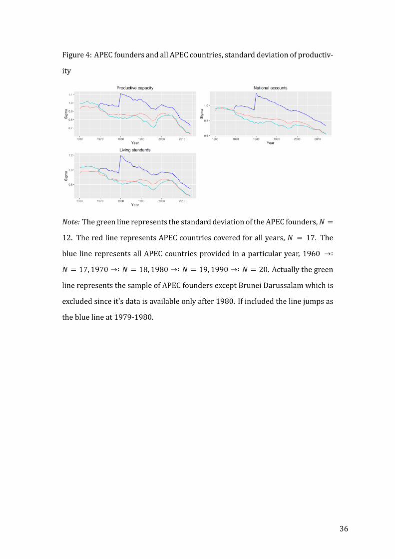
Figure 4: APEC founders and all APEC countries, standard deviation of productiv-
ity
Note: The green line represents the standard deviation of the APEC founders,𝑁 =
12. The red line represents APEC countries covered for all years, 𝑁 = 17. The
blue line represents all APEC countries provided in a particular year, 1960 →∶
𝑁 = 17, 1970 →∶ 𝑁 = 18, 1980 →∶ 𝑁 = 19, 1990 →∶ 𝑁 = 20. Actually the green
line represents the sample of APEC founders except Brunei Darussalam which is
excluded since it’s data is available only after 1980. If included the line jumps as
the blue line at 1979-1980.
36

Figure 5: OECD, EU and APEC, standard deviation of productivity
Note: The red line represents OECD, APEC and EU countries covered for all years,
𝑁 = 40. The blue line represents all OECD, APEC and EU countries provided in a
particular year, 1960 →∶ 𝑁 = 40, 1970 →∶ 𝑁 = 44, 1980 →∶ 𝑁 = 45, 1990 →∶
𝑁 = 53.
37

Figure 6: All countries vs. OECD, EU and APEC, 𝛽-convergence
Note: All (red dots and blue dots): 𝑁 = 82, 103, 142, 166, 169; OECD, EU and
APEC (blue dots): 𝑁 = 40, 44, 45, 53, 53.
38

Figure 7: Africa, standard deviation of productivity
Note: The red line represents countries of Africa covered for all years, 𝑁 = 22.
The blue line represents all countries of Africa provided in a particular year,
1960 →∶ 𝑁 = 22, 1970 →∶ 𝑁 ≃ 24, 1980 →∶ 𝑁 ≃ 49, 2000 →∶ 𝑁 = 50.
39

Figure 8: Asia, standard deviation of productivity
Note: The red line represents countries of Asia covered for all years,𝑁 = 19. The
blue line represents all countries of Asia provided in a particular year, 1960 →∶
𝑁 ≃ 19, 1970 →∶ 𝑁 = 29, 1980 →∶ 𝑁 ≃ 36,1990 →∶ 𝑁 ≃ 46.
40

Figure 9: Europe, standard deviation of productivity
Note: The red line represents countries of Europe covered for all years, 𝑁 = 21.
The blue line represents all countries of Europe provided in a particular year,
1960 →∶ 𝑁 = 21, 1970 →∶ 𝑁 = 25, 1990 →∶ 𝑁 = 40.
41

Figure 10: Europe - East and West, National accounts GDP, 𝛽-regression
Note: East Europe (red): 𝑁 = 20; West Europe (blue): 𝑁 = 20.
42

Figure 11: South America, standard deviation of productivity
Note: The red line represents countries of South America covered for all years,
𝑁 = 9. The blue line represents all countries of South America provided in a
particular year, 1960 →∶ 𝑁 = 9, 1970 →∶ 𝑁 = 10, 1980 →∶ 𝑁 = 11.
43
Figure 12: All vs. Continents, National accounts GDP, 𝛽-convergence
Note: All (blue line, all dots), Africa (red), Asia (green), Europe (purple), South
America (orange).
44

Table 1: World 𝜎-tests
World 1960-2014 1970-2014 1980-2014 1990-2014 2000-2014
Prod. cap. Adjusted ROV -2.38 (0.99) 0.77 (0.22) 0.16 (0.44) -0.20 (0.58) 1.56 (0.06)
Likelihood 4.00 (0.05) 0.63 (0.43) 0.03 (0.87) 0.04 (0.84) 3.52 (0.06)
Wald 4.55 (0.03) 0.48 (0.49) 0.02 (0.89) 0.03 (0.86) 2.57 (0.11)
Liv. stand. Adjusted ROV -3.64 (1.00) 0.03 (0.49) 0.21 (0.42) -0.72 (0.76) 1.42 (0.08)
Likelihood 6.41 (0.01) 0 (0.97) 0.05 (0.83) 0.44 (0.51) 2.91 (0.09)
Wald 7.62 (0.01) 0 (0.98) 0.03 (0.86) 0.36 (0.55) 2.04 (0.15)
Nat. Acc. Adjusted ROV -1.86 (0.97) 1.81 (0.03) 1.61 (0.05) 1.12 (0.13) 2.34 (0.01)
Likelihood 2.47 (0.12) 3.68 (0.05) 3.24 (0.07) 1.62 (0.20) 12.19 (0.00)
Wald 2.57 (0.11) 2.5 (0.11) 2.06 (0.15) 1.22 (0.27) 8.69 (0.00)
N 82 103 142 166 169
Note: The statistics of the 𝜎-tests and the associated 𝑝-values in parenthesis.
45

Table 2: OECD countries 𝜎-tests
OECD 1960-2014 1970-2014 1980-2014 1990-2014 2000-2014
Prod. cap. Adjusted ROV 6.68 (0.00) 5.31 (0.00) 3.08 (0.00) 2.37 (0.01) 2.46 (0.01)
Likelihood 10.29 (0.00) 8.78 (0.00) 4.88 (0.03) 4.49 (0.03) 6.85 (0.01)
Wald 48.35 (0.00) 46.14 (0.00) 33.73 (0.00) 37.45 (0.00) 60.89 (0.00)
Liv. stand. Adjusted ROV 7.88 (0.00) 6.7 (0.00) 4.39 (0.00) 3.62 (0.00) 3.43 (0.00)
Likelihood 12.62 (0.00) 12.15 (0.00) 8.29 (0.00) 9.35 (0.00) 12.27 (0.00)
Wald 59.8 (0.00) 64.83 (0.00) 55.61 (0.00) 79.72 (0.00) 117.43 (0.00)
Nat. Acc. Adjusted ROV 5.74 (0.00) 4.34 (0.00) 2.75 (0.00) 3.48 (0.00) 2.34 (0.01)
Likelihood 9.81 (0.00) 8.11 (0.00) 4.88 (0.03) 10.87 (0.00) 9.41 (0.00)
Wald 49.6 (0.00) 47.12 (0.00) 35.28 (0.00) 80.42 (0.00) 86.79 (0.00)
N 28 30 30 34 34
Note: The statistics of the 𝜎-tests and the associated 𝑝-values in parenthesis.
46

Table 3: EU all countries, 𝜎-tests
EU 1960-2014 1970-2014 1980-2014 1990-2014 2000-2014
Prod. cap. Adjusted ROV 22.04 (0.00) 8.38 (0.00) 4.09 (0.00) 4.05 (0.00) 5.48 (0.00)
Likelihood 30.28 (0.00) 19.45 (0.00) 8.75 (0.00) 10.14 (0.00) 16.8 (0.00)
Wald 174.76 (0.00) 91.33 (0.00) 50.69 (0.00) 71.02 (0.00) 111.78 (0.00)
Liv. stand. Adjusted ROV 20.69 (0.00) 9.57 (0.00) 5.20 (0.00) 5.36 (0.00) 7.03 (0.00)
Likelihood 32.24 (0.00) 24.13 (0.00) 14.03 (0.00) 16.33 (0.00) 27.12 (0.00)
Wald 252.37 (0.00) 124.79 (0.00) 85.89 (0.00) 116.18 (0.00) 203.55 (0.00)
Nat. Acc. Adjusted ROV 11.86 (0.00) 6.65 (0.00) 2.65 (0.00) 4.64 (0.00) 5.08 (0.00)
Likelihood 20.00 (0.00) 18.64 (0.00) 6.85 (0.01) 16.78 (0.00) 19.94 (0.00)
Wald 129.28 (0.00) 103.13 (0.00) 50.34 (0.00) 124.38 (0.00) 149.33 (0.00)
N 18 21 21 28 28
Note: The statistics of the 𝜎-tests and the associated 𝑝-values in parenthesis.
47
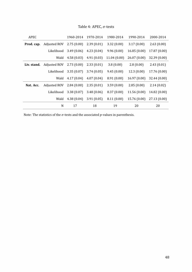
Table 4: APEC, 𝜎-tests
APEC 1960-2014 1970-2014 1980-2014 1990-2014 2000-2014
Prod. cap. Adjusted ROV 2.75 (0.00) 2.39 (0.01) 3.32 (0.00) 3.17 (0.00) 2.63 (0.00)
Likelihood 3.49 (0.06) 4.23 (0.04) 9.96 (0.00) 16.85 (0.00) 17.87 (0.00)
Wald 4.58 (0.03) 4.91 (0.03) 11.04 (0.00) 26.07 (0.00) 32.39 (0.00)
Liv. stand. Adjusted ROV 2.73 (0.00) 2.33 (0.01) 3.8 (0.00) 2.8 (0.00) 2.43 (0.01)
Likelihood 3.35 (0.07) 3.74 (0.05) 9.45 (0.00) 12.3 (0.00) 17.76 (0.00)
Wald 4.17 (0.04) 4.07 (0.04) 8.91 (0.00) 16.97 (0.00) 32.44 (0.00)
Nat. Acc. Adjusted ROV 2.84 (0.00) 2.35 (0.01) 3.59 (0.00) 2.85 (0.00) 2.14 (0.02)
Likelihood 3.38 (0.07) 3.48 (0.06) 8.37 (0.00) 11.56 (0.00) 14.82 (0.00)
Wald 4.38 (0.04) 3.91 (0.05) 8.11 (0.00) 15.76 (0.00) 27.13 (0.00)
N 17 18 19 20 20
Note: The statistics of the 𝜎-tests and the associated 𝑝-values in parenthesis.
48

Table 5: OECD, EU and APEC, 𝜎-tests
OECD, EU, APEC 1960-2014 1970-2014 1980-2014 1990-2014 2000-2014
Prod. cap. Adjusted ROV 5.68 (0.00) 4.2 (0.00) 4.45 (0.00) 4.48 (0.00) 4.44 (0.00)
Likelihood 13.85 (0.00) 13.5 (0.00) 19.44 (0.00) 27.55 (0.00) 33.44 (0.00)
Wald 24.79 (0.00) 23.98 (0.00) 36.03 (0.00) 67.02 (0.00) 88.24 (0.00)
Liv. stand. Adjusted ROV 5.42 (0.00) 4.59 (0.00) 5.26 (0.00) 4.43 (0.00) 4.39 (0.00)
Likelihood 13.29 (0.00) 15.21 (0.00) 21.85 (0.00) 27.21 (0.00) 36.08 (0.00)
Wald 23.98 (0.00) 25.5 (0.00) 36.59 (0.00) 65.03 (0.00) 97.03 (0.00)
Nat. Acc. Adjusted ROV 5.38 (0.00) 4.67 (0.00) 5.15 (0.00) 4.82 (0.00) 3.97 (0.00)
Likelihood 13.17 (0.00) 15.44 (0.00) 21.89 (0.00) 33.89 (0.00) 36.03 (0.00)
Wald 25.68 (0.00) 27.47 (0.00) 38.98 (0.00) 87.09 (0.00) 107.99 (0.00)
N 40 44 45 53 53
Note: The statistics of the 𝜎-tests and the associated 𝑝-values in parenthesis.
49

Table 6: World, OECD, EU and APEC, 𝛽-convergence (NLS)
1960-2014 1970-2014 1980-2014 1990-2014 2000-2014
World Prod. cap. -0.002 -0.004*** -0.004*** -0.005** -0.008***
Liv. stand. -0.001 -0.004** -0.004*** -0.004* -0.007***
Nat. acc. -0.002* -0.005*** -0.005*** -0.004*** -0.007***
N 82 103 142 166 169
OECD Prod. cap. -0.011*** -0.013*** -0.014*** -0.014*** -0.019***
Liv. stand. -0.011*** -0.012*** -0.014*** -0.015*** -0.022***
Nat. acc. -0.010*** -0.011*** -0.012*** -0.014*** -0.016***
N 28 30 30 34 34
OECD founders Prod. cap. -0.011*** -0.013*** -0.013*** -0.014*** -0.017**
Liv. stand. -0.010*** -0.011*** -0.013*** -0.014*** -0.019***
Nat. acc. -0.009*** -0.008*** -0.009*** -0.007** -0.009*
N 20 20 20 20 20
EU Prod. cap. -0.011*** -0.011*** -0.012*** -0.016*** -0.029***
Liv. stand. -0.010*** -0.011*** -0.012*** -0.017*** -0.03***
Nat. acc. -0.010*** -0.010*** -0.009*** -0.015*** -0.026***
N 18 21 21 28 28
EU core Prod. cap. -0.011*** -0.014*** -0.016*** -0.017*** -0.026***
Liv. stand. -0.010*** -0.011*** -0.013*** -0.015*** -0.021***
Nat. acc. -0.009*** -0.010*** -0.010*** -0.009 -0.005
N 15 15 15 15 15
APEC Prod. cap. -0.008*** -0.008*** -0.010*** -0.012*** -0.017***
Liv. stand. -0.009*** -0.008*** -0.011*** -0.011*** -0.016***
Nat. acc. -0.009*** -0.009*** -0.011*** -0.012*** -0.015***
N 17 18 19 20 20
APEC founders Prod. cap. -0.008*** -0.008*** -0.010*** -0.010*** -0.016***
Liv. stand. -0.008*** -0.009*** -0.012*** -0.011*** -0.014***
Nat. acc. -0.008*** -0.008*** -0.012*** -0.011*** -0.013***
N 12 12 13 13 13
OECD, EU and APEC Prod. cap. -0.009*** -0.008*** -0.010*** -0.012*** -0.019***
Liv. stand. -0.009*** -0.008*** -0.011*** -0.012*** -0.019***
Nat. acc. -0.009*** -0.009*** -0.010*** -0.012*** -0.017***
N 40 44 45 53 53
Note: The estimates are from the NLS 𝛽-regressions (3). The signi icance levels are appointed accord-
ingly: 0.1∗, 0.05∗∗, 0.01∗∗∗. The standard errors of the coef icients (not shown) are heteroscedasticity
robust (White, 1980) whereas the associated 𝑝-values are from the 𝑇 distribution with 𝑁 − 2 degrees
of freedom.
50

Table 7: Africa, 𝜎-tests
Africa 1960-2014 1970-2014 1980-2014 1990-2014 2000-2014
Prod. cap. Adjusted ROV -0.22 (0.59) -0.68 (0.75) -2.10 (0.98) -1.19 (0.88) -1.05 (0.85)
Likelihood 0.04 (0.84) 0.35 (0.56) 3.00 (0.08) 1.25 (0.26) 0.65 (0.42)
Wald 0.05 (0.82) 0.46 (0.50) 4.02 (0.04) 1.47 (0.23) 0.64 (0.42)
Liv. stand. Adjusted ROV -0.77 (0.78) -1.10 (0.86) -2.31 (0.99) -1.38 (0.92) -0.91 (0.82)
Likelihood 0.50 (0.48) 0.74 (0.39) 3.41 (0.06) 1.62 (0.20) 0.53 (0.47)
Wald 0.70 (0.40) 1.05 (0.30) 4.60 (0.03) 1.93 (0.17) 0.51 (0.48)
Nat. Acc. Adjusted ROV -0.35 (0.64) -0.02 (0.51) -1.61 (0.95) -0.74 (0.77) -0.06 (0.53)
Likelihood 0.10 (0.75) 0.00 (0.99) 1.42 (0.23) 0.40 (0.53) 0.00 (0.95)
Wald 0.12 (0.73) 0.00 (0.98) 1.54 (0.21) 0.39 (0.53) 0.00 (0.95)
N 22 24 49 49 50
Note: The statistics of the 𝜎-tests and the associated 𝑝-values in parenthesis.
51

Table 8: Asia, 𝜎-tests
Asia 1960-2014 1970-2014 1980-2014 1990-2014 2000-2014
Prod. cap. Adjusted ROV -0.66 (0.74) 4.51 (0.00) 4.85 (0.00) 2.44 (0.01) 2.61 (0.00)
Likelihood 0.39 (0.53) 13.13 (0.00) 26.37 (0.00) 8.41 (0.00) 12.42 (0.00)
Wald 0.90 (0.34) 7.56 (0.01) 17.91 (0.00) 7.24 (0.01) 10.46 (0.00)
Liv. stand. Adjusted ROV -1.00 (0.84) 3.66 (0.00) 5.03 (0.00) 1.81 (0.03) 2.29 (0.01)
Likelihood 0.88 (0.35) 9.62 (0.00) 23.66 (0.00) 4.12 (0.04) 9.55 (0.00)
Wald 2.17 (0.14) 5.73 (0.02) 14.25 (0.00) 3.44 (0.06) 7.65 (0.01)
Nat. Acc. Adjusted ROV 0.97 (0.17) 5.91 (0.00) 5.88 (0.00) 3.49 (0.00) 3.02 (0.00)
Likelihood 0.66 (0.42) 19.03 (0.00) 28.45 (0.00) 19.51 (0.00) 17.84 (0.00)
Wald 0.88 (0.35) 9.95 (0.00) 16.68 (0.00) 15.95 (0.00) 14.55 (0.00)
N 19 29 36 45 46
Note: The statistics of the 𝜎-tests and the associated 𝑝-values in parenthesis.
52

Table 9: Europe, 𝜎-tests
Europe 1960-2014 1970-2014 1980-2014 1990-2014 2000-2014
Prod. cap. Adjusted ROV 17.71 (0.00) 6.25 (0.00) 3.71 (0.00) 3.83 (0.00) 5.42 (0.00)
Likelihood 27.31 (0.00) 15.61 (0.00) 9.13 (0.00) 9.12 (0.00) 32.19 (0.00)
Wald 120.78 (0.00) 59.19 (0.00) 42.71 (0.00) 28.11 (0.00) 120.1 (0.00)
Liv. stand. Adjusted ROV 21.03 (0.00) 7.84 (0.00) 4.99 (0.00) 2.99 (0.00) 5.71 (0.00)
Likelihood 33.26 (0.00) 22.32 (0.00) 16.01 (0.00) 7.02 (0.01) 42.59 (0.00)
Wald 226.96 (0.00) 94.33 (0.00) 82.06 (0.00) 22.7 (0.00) 169.52 (0.00)
Nat. Acc. Adjusted ROV 10.09 (0.00) 5.49 (0.00) 3.14 (0.00) 3.52 (0.00) 4.94 (0.00)
Likelihood 20.53 (0.00) 18.92 (0.00) 12.14 (0.00) 10.11 (0.00) 35.97 (0.00)
Wald 106.98 (0.00) 81.23 (0.00) 65.2 (0.00) 33.67 (0.00) 151.33 (0.00)
N 21 25 25 40 40
Note: The statistics of the 𝜎-tests and the associated 𝑝-values in parenthesis.
53

Table 10: South America, 𝜎-tests
1960-2014 1970-2014 1980-2014 1990-2014 2000-2014
Prod. cap. Adjusted ROV 0.83 (0.2) 1.10 (0.14) 0.54 (0.29) 0.66 (0.26) 1.29 (0.10)
Likelihood 0.41 (0.52) 0.79 (0.37) 0.22 (0.64) 0.41 (0.52) 3.73 (0.05)
Wald 1.60 (0.21) 2.80 (0.09) 0.97 (0.32) 1.82 (0.18) 17.47 (0.00)
Liv. stand. Adjusted ROV 1.53 (0.06) 1.51 (0.07) 0.71 (0.24) 0.82 (0.21) 1.31 (0.10)
Likelihood 1.20 (0.27) 1.37 (0.24) 0.37 (0.54) 0.59 (0.44) 3.65 (0.06)
Wald 3.90 (0.05) 4.49 (0.03) 1.54 (0.21) 2.51 (0.11) 16.83 (0.00)
Nat. Acc. Adjusted ROV 0.25 (0.40) 1.05 (0.15) 0.01 (0.49) 0.66 (0.26) 1.13 (0.13)
Likelihood 0.04 (0.83) 0.82 (0.36) 0.00 (0.99) 0.38 (0.54) 2.99 (0.08)
Wald 0.22 (0.64) 3.03 (0.08) 0.00 (0.98) 1.73 (0.19) 14.6 (0.00)
N 9 10 11 11 11
Note: The statistics of the 𝜎-tests and the associated 𝑝-values in parenthesis.
54

Table 11: Continents, 𝛽-convergence (NLS)
1960-2014 1970-2014 1980-2014 1990-2014 2000-2014
Africa Prod. cap. -0.005*** -0.003** -0.004 -0.008 -0.004
Liv. stand. -0.004* -0.002 -0.003 -0.008 -0.005
Nat. acc. -0.003*** -0.003** -0.002 -0.004* -0.003
N 22 24 49 49 50
Asia Prod. cap. -0.005** -0.009*** -0.010*** -0.010*** -0.015***
Liv. stand. -0.004* -0.008*** -0.010*** -0.009*** -0.014***
Nat. acc. -0.008*** -0.009*** -0.011*** -0.011*** -0.016***
N 19 29 36 45 46
Europe Prod. cap. -0.010*** -0.010*** -0.011*** -0.017*** -0.024***
Liv. stand. -0.010*** -0.010*** -0.011*** -0.015*** -0.024***
Nat. acc. -0.009*** -0.009*** -0.009*** -0.014*** -0.022***
N 21 25 25 40 40
South America Prod. cap. -0.007** -0.008** -0.009** -0.009** -0.013**
Liv. stand. -0.007** -0.008*** -0.009** -0.010** -0.014**
Nat. acc. -0.004 -0.007* -0.004 -0.010* -0.012**
N 9 10 11 11 11
ASEAN Prod. cap. -0.003 -0.001 -0.009*** -0.01*** -0.014***
Liv. stand. -0.003 0 -0.01*** -0.009*** -0.014***
Nat. acc. -0.006 -0.002 -0.01*** -0.011*** -0.015***
N 5 8 10 10 10
South and Middle Am. Prod. cap. -0.008*** -0.007*** -0.013*** -0.016*** -0.015*
Liv. stand. -0.008*** -0.008*** -0.013*** -0.015*** -0.014*
Nat. acc. -0.004 -0.005* -0.001 -0.003 -0.004
N 12 15 19 19 19
Eurasia Prod. cap. -0.006*** -0.009*** -0.009*** -0.01*** -0.017***
Liv. stand. -0.006*** -0.008*** -0.009*** -0.009*** -0.016***
Nat. acc. -0.007*** -0.009*** -0.01*** -0.011*** -0.016***
40 54 61 85 86
World without Africa Prod. cap. -0.007*** -0.008*** -0.008*** -0.01*** -0.016***
Liv. stand. -0.007*** -0.007*** -0.009*** -0.009*** -0.015***
Nat. acc. -0.007*** -0.008*** -0.009*** -0.009*** -0.014***
N 60 79 93 117 119
Note: The estimates are from the NLS 𝛽-regressions (3). The signi icance levels are appointed accord-
ingly: 0.1∗, 0.05∗∗, 0.01∗∗∗. The standard errors of the coef icients (not shown) are heteroscedasticity ro-
bust (White, 1980) whereas the associated 𝑝-values are from the 𝑇 distribution with 𝑁 − 2 degrees of
freedom. 55

A Appendix
Table 12: Country groups 1
OECD OECD founders EU Core EU EU canditates Apec Apec founders
Australia - Austria Austria Albania Australia Australia
Austria Austria Belgium Belgium Iceland Brunei Darussalam Brunei Darussalam
Belgium Belgium Bulgaria - Macedonia Canada Canada
Canada Canada Croatia - Montenegro Chile -
Chile - Cyprus - Serbia Hong Kong -
Czech Republic - Czech Republic - Turkey Indonesia Indonesia
Denmark Denmark Denmark Denmark Japan Japan
Estonia - Estonia - Former Eastern bloc Malaysia Malaysia
Finland - Finland Finland Albania Mexico -
France France France France Belarus New Zealand New Zealand
Germany Germany Germany Germany Bosnia and Herzegovina People’s Republic of China -
Greece Greece Greece Greece Bulgaria Peru -
Hungary - Hungary - Croatia Philippines Philippines
Iceland Iceland Ireland Ireland Czech Republic Russian Federation -
Ireland Ireland Italy Italy Estonia Singapore Singapore
Israel - Latvia - Hungary South Korea South Korea
Italy Italy Lithuania - Latvia Thailand Thailand
Japan - Luxembourg Luxembourg Lithuania United States United States
Korea - Malta - Macedonia Vietnam -
Luxembourg Luxembourg Netherlands Netherlands Moldova Taiwan -
Mexico - Poland - Montenegro
Netherlands Netherlands Portugal Portugal Poland Excluded since no data
New Zealand - Romania - Romania Papua New Guinea
Norway Norway Slovakia - Russia
Poland - Slovenia - Serbia
Portugal Portugal Spain Spain Slovakia
Slovakia - Sweden Sweden Slovenia
Slovenia - United Kingdom United Kingdom Ukraine
Spain Spain
Sweden Sweden
Switzerland Switzerland
Turkey Turkey
United Kingdom United Kingdom
United States United States
𝑁 = 34 𝑁 = 20 𝑁 = 28 𝑁 = 15 𝑁 = 6, 𝑁 = 20 𝑁 = 21 𝑁 = 13
56

Table 13: Country groups 2
Afrika Asia Europe South America Not included
Armenia Austria Argentina Australia
North-South-West Azerbaijan Belgium Bolivia Fiji
Algeria Bahrain Cyprus Brazil New Zealand
Benin Bangladesh Denmark Chile
Botswana Bhutan Finland Colombia Canada
Burkina Faso China France Ecuador United States
Cape Verde Islands Georgia Germany Paraguay
Egypt Hong Kong Greece Peru
Gambia India Iceland Suriname
Ghana Iran Ireland Uruguay
Guinea Iraq Italy Venezuela
Guinea-Bissau Israel Luxembourg
Ivory Coast Japan Malta Middle America
Lesotho Jordan Netherlands Belize
Liberia Kazakhstan Norway Costa Rica
Mali Republic South Korea Portugal El Salvador
Mauritania Kuwait Spain Guatemala
Morocco Kyrgyzstan Sweden Honduras
Namibia Lebanon Switzerland Mexico
Niger Republic Macau United Kingdom Nicaragua
Nigeria Maldives Panama
Senegal Republic Mongolia East-Europe
Sierra Leone Nepal Albania Middle (islands)
South Africa Oman Belarus Anguilla
Sudan Pakistan Bosnia and Herzegovina Antigua and Barbuda
Swaziland Qatar Bulgaria Aruba
Togo Saudi Arabia Croatia Bahamas
Tunisia Sri Lanka Czech Republic Barbados
State of Palestine Estonia Bermuda
East-Central Syria Hungary British Virgin Islands
Angola Taiwan Latvia Cayman Islands
Burundi Tajikistan Lithuania Curacao
Cameroon Turkey Macedonia Dominica
Central African Republic Turkmenistan Moldova Dominican Republic
Chad Republic United Arab Emirates Montenegro Grenada
Comoros Uzbekistan Poland Haiti
Congo Yemen Romania Jamaica
Dem. Republic of the Congo Russia Montserrat
Djibouti ASEAN Serbia Saint Kitts and Nevis
Equatorial Guinea Brunei Slovakia Saint Lucia
Ethiopia Cambodia Slovenia Sint Maarten
Gabon Republic Indonesia Ukraine St. Vincent and the Grenadines
Kenya Laos Ukraine Trinidad and Tobago
Madagascar Malaysia Turks and Caicos Islands
Malawi Myanmar
Mauritius Philippines
Mozambique Singapore
Rwanda Thailand
Sao Tome and Principe Vietnam
Seychelles
Tanzania
Uganda
Zambia
Zimbabwe
𝑁 = 50 𝑁 = 47 𝑁 = 40 𝑁 = 40 𝑁 = 5
1 Note: For Anguilla, Antigua and Barbuda, Bermuda, British Virgin Islands, Cayman Islands, Curacao, Dominica, Grenada,
Montserrat, Saint Kitts andNevis, SintMaarten andTurks andCaicos Islands employment data is short of necessary yearsmainly
2014.
57
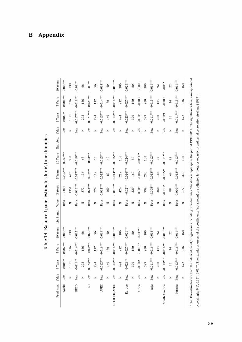
B Appendix
Table1
4:Ba
lancedp
anelestim
ates
for𝛽
,timed
ummies
Prod
.cap
.Va
lue
3Years
5Years
10Years
Liv.Stan
d.Va
lue
3Years
5Years
10Years
Nat.Ac
c.Va
lue
3Years
5Years
10Years
World
Beta
-0.00
4**
-0.00
7***
-0.00
8***
Beta
-0.00
3-0.00
5***
-0.00
7***
Beta
-0.00
3**
-0.00
6***
-0.00
6***
N13
5167
633
8N
1351
676
338
N13
5167
633
8
OECD
Beta
-0.01
6**
-0.01
4***
-0.01
5***
Beta
-0.01
9***
-0.01
7***
-0.01
9***
Beta
-0.01
7***
-0.01
9***
-0.02
***
N27
213
668
N27
213
668
N27
213
668
EUBe
ta-0.02
3***
-0.03
***
-0.02
9***
Beta
-0.02
4***
-0.03
***
-0.03
***
Beta
-0.02
1***
-0.02
9***
-0.03
***
N22
411
256
N22
411
256
N22
411
256
APEC
Beta
-0.01
2***
-0.01
6***
-0.01
4***
Beta
-0.01
1***
-0.01
3***
-0.01
3***
Beta
-0.01
3***
-0.01
4***
-0.01
3***
N16
080
40N
160
8040
N16
080
40
OECD
,EU,
APEC
Beta
-0.01
4***
-0.01
6***
-0.01
6***
Beta
-0.01
3***
-0.01
4***
-0.01
5***
Beta
-0.01
4***
-0.01
6***
-0.01
6***
N42
421
210
6N
424
212
106
N42
421
210
6
Europe
Beta
-0.02
6**
-0.02
7***
-0.02
4***
Beta
-0.02
**-0.02
6***
-0.02
4***
Beta
-0.02
3***
-0.02
7***
-0.02
6***
N32
016
080
N32
016
080
N32
016
080
Afric
aBe
ta-0.00
2-0.00
8**
-0.01
2**
Beta
0.001
-0.00
7*-0.01
1**
Beta
-0.00
1-0.00
3-0.00
5
N39
920
010
0N
399
200
100
N39
920
010
0
Asia
Beta
-0.01
1***
-0.01
6***
-0.01
3***
Beta
-0.00
8**
-0.01
3***
-0.01
2***
Beta
-0.01
1***
-0.01
5***
-0.01
4***
N36
818
492
N36
818
492
N36
818
492
SouthA
merica
Beta
-0.01
3***
-0.01
6***
-0.01
0***
Beta
-0.01
3*-0.01
5**
-0.01
1***
Beta
-0.00
9-0.00
9-0.01
*
N88
4422
N88
4422
N88
4422
Eurasia
Beta
-0.01
2***
-0.01
6***
-0.01
4***
Beta
-0.00
9***
-0.01
3***
-0.01
3***
Beta
-0.01
1***
-0.01
5***
-0.01
4***
N67
233
616
8N
672
336
168
N67
233
616
8
Note:T
heestim
ates
aref
rom
theb
alanc
edpa
nel𝛽
-regressio
nsinclu
ding
timed
ummies
.The
data
samples
pans
thep
eriod1
990-20
14.T
hesig
niica
ncelevels
area
ppointed
accordingly
:0.1∗
,0.05
∗∗,0.01
∗∗∗ .Th
estand
ards
errors
ofthec
oeficie
nts(
notsho
wn)a
read
juste
dfor
heterosked
astic
ityan
dserial
correla
tionA
rella
no(198
7).
58

Table1
5:Pa
nelesti
mates
for𝛽
,timed
ummies
Prod
.cap
.Va
lue
3Years
5Years
10Years
Liv.Stan
d.Va
lue
3Years
5Years
10Years
Nat.Ac
c.Va
lue
3Years
5Years
10Years
World
Beta
-0.00
3*-0.00
5***
-0.00
5***
Beta
-0.00
2-0.00
4**
-0.00
4***
Beta
-0.00
3**
-0.00
3***
-0.00
4***
N24
4614
1866
9N
2446
1418
669
N24
4614
1866
9
OECD
Beta
-0.02
1***
-0.02
2***
-0.02
2***
Beta
-0.02
2***
-0.02
2***
-0.02
2***
Beta
-0.01
7***
-0.01
6***
-0.01
7***
N56
631
815
6N
566
318
156
N56
631
815
6
EUBe
ta-0.01
7***
-0.02
0***
-0.02
2***
Beta
-0.02
2***
-0.01
9***
-0.02
1***
Beta
-0.02
1***
-0.01
7***
-0.02
1***
N42
524
211
6N
425
242
116
N42
524
211
6
APEC
Beta
-0.00
8***
-0.01
2***
-0.01
1***
Beta
-0.00
9***
-0.01
4***
-0.01
3***
Beta
-0.00
9***
-0.01
2***
-0.01
2***
N34
019
194
N34
019
194
N34
019
194
OECD
,EU,
APEC
Beta
-0.00
9***
-0.01
2***
-0.01
2***
Beta
-0.01
1***
-0.01
3***
-0.01
3***
Beta
-0.01
0***
-0.01
1***
-0.01
2***
N85
548
323
5N
855
483
235
N85
548
323
5
Europe
Beta
-0.01
9***
-0.01
9***
-0.02
1***
Beta
-0.01
9***
-0.01
5***
-0.01
9***
Beta
-0.01
9***
-0.01
4***
-0.01
9***
N55
832
115
1N
558
321
151
N55
832
115
1
Afric
aBe
ta-0.00
1-0.00
4-0.00
7**
Beta
0.001
-0.00
3-0.00
6*Be
ta0.0
000.0
00-0.00
2
N70
941
719
5N
709
417
195
N70
941
719
5
Asia
Beta
-0.01
1***
-0.01
6***
-0.01
5***
Beta
-0.01
***
-0.01
5***
-0.01
5***
Beta
-0.01
2***
-0.01
2***
-0.01
4***
N65
137
917
7N
651
379
177
N65
137
917
7
SouthA
merica
Beta
-0.01
3**
-0.01
3**
-0.01
1*Be
ta-0.01
3**
-0.01
4**
-0.01
3**
Beta
-0.01
0-0.00
9*-0.00
9
N19
110
753
N19
110
753
N19
110
753
Eurasia
Beta
-0.01
0***
-0.01
2***
-0.01
2***
Beta
-0.00
9***
-0.01
1***
-0.01
2***
Beta
-0.01
1***
-0.01
1***
-0.01
2***
N11
7768
131
9N
1177
681
319
N11
7768
131
9
Note:T
heestim
ates
arefromtheu
nbala
nced
pane
l𝛽-re
gressio
nsinclu
ding
timed
ummies
.The
datasamples
pans
thep
eriod1
960-20
14.T
hesig
niica
ncelevels
area
ppointed
accordingly
:0.1∗
,0.05
∗∗,0.01
∗∗∗ .Th
estand
ards
errors
ofthec
oeficie
nts(
notsho
wn)a
read
juste
dfor
heterosked
astic
ityan
dserial
correla
tionA
rella
no(198
7).
59


