Traditional Elites: Agricultural Productivity

and the Persistence of Political Power

Please find latest version: Here

SABRIN BEG1

Abstract

I study the historic presence of landed elites in Pakistan, and the effect of apermanent shift in agricultural productivity on their persistence. First, I usehousehold data to document that agricultural landowners can make transfersto sharecropping tenants at a relatively low cost, thereby gaining tenants’electoral support and swaying public policy in their favor. I exploit a regimechange from non-democratic to democratic; after elections politician land-lords offer concessions on input costs to their sharecroppers. In the presenceof moral hazard, technological change in agriculture makes sharecropping lessoptimal, attenuating landlords’ electoral advantage. For plausibly exogenousvariation in agricultural productivity I use introduction of high yielding va-riety (HYV) seeds in combination with agro-ecological suitability for HYVs.I find that increased productivity lowers the rate of sharecropping and low-ers the likelihood of election of landlords in historically landlord-dominatedareas; in turn there is an improvement in electoral competition and a shiftin the composition of public goods away from those preferred by agriculturallandowners. Agricultural productivity gives way to the transformation of theidentity of political elites.

Keywords: Land Inequality; Clientelism; Public Goods; Colonial Institutions;Electoral Competition, Traditional Chiefs; Political Economy; Elite Capture.

1University of Delaware (e-mail: sabrin.beg@gmail.com)I would like to thank Mark Rosenzweig, Christopher Udry, Dan Keniston, Nancy Qian, David

Atkin, Eric Weese and Dean Karlan for advice and support. I would also like to thank LauraSchechter, Asim Khwaja, Ali Cheema, Naved Hamid, Alexander Debs, Susan Hyde, Kate Balwin,Raul Sanchez de la Sierra, Thomas Kirk and participants at the Yale Development Seminar, LeitnerPolitical Economy seminar, Princeton and Boston University for helpful feedback and comments.I am thankful to fellow graduate students for helpful discussions and to Rahul Deb, Yingni Guoand Shameel Ahmad for editorial and technological comments. I thank Jacob Shapiro and AbdulGhaffar for useful data, without which this project would not have been possible. I acknowledgefinancial support from the Sylff Foundation and Georg W. Leitner Program in International andComparative Political Economy. All errors are mine.

1

1 Introduction

Colonial history undoubtedly shapes current economic outcomes;2 the effects

of historic inequality, in particular, can persist through channels such as hu-

man capital investment, property rights and public goods (Galor, Moav and

Vollrath 2003, 2009, Engerman and Sokoloff 2005, 2007, Banerjee and Iyer

2001). Another potential channel is the identity and incentives of political

elites. The initial distribution of assets, particularly land, determines the dis-

tribution of political power and the identity of policy makers, which in turn

determines the provision of public goods. In this paper, I examine the mech-

anisms through which colonial landed elites can influence the postcolonial

distribution of political power, and ultimately public policy and subsequent

development. Economic growth, in turn, can reinforce or undermine the power

of these elites; I examine the impact of agricultural development on the politi-

cal dominance of landowning elites and the consequent implications for public

goods provision.

The intersection of land ownership, paternalism and power is central to

development throughout history; indeed several societies in history, including

the Roman Empire, medieval Europe, traditional societies in Latin America

and East Asia, and the pre-industrial United States South have witnessed

landlords dominating the politico-economic environment. Across varied con-

texts, powerful landlords are known to have controlled the peasantry, but also

provided patronage and public goods to them.3 As patrons, the landlords pre-

clude the provision of broad welfare by the state. Indeed, the rapid growth in

East Asia has been attributed in part to extensive land reforms, which facil-

itated eliminating the landlord class and providing the basis for an equitable

distribution of the benefits of growth (Grabowski 2002). The decline of land-

lords’ power led way for the formation of national welfare states by breaking

down the paternalistic ties between landlords and their rural clients. In this

paper I theoretically identify and test the micro-foundations that define the

initial patron-client relationship between the landlord and sharecropper, and

the eventual shift in equilibrium that follows from the technological changes

in agriculture using the context of Pakistan.

2See Nunn 2009, Glaeser and Shleifer 2002, Acemoglu, Johnson, and Robinson 2001,20023Chile in Baland and Robinson 2012; pre-industrial Europe in Brenner 1976; US South in Alston

and Ferrie 1999; Peru in Dell 2012

2

Specifically, I pose three major questions: first, how do historic landown-

ing elites acquire and maintain political power? Second, how does the inter-

action of land and power affect electoral competition and the provision of

public goods? Lastly, how does landlords’ ability to acquire political support

shift with a permanent, exogenous improvement in agricultural productivity

and what are the consequent implications for electoral and public goods out-

comes? The paper presents new micro-founded mechanisms to understand

the impact of historic land institutions and land inequality on development

outcomes. Moreover, it highlights the processes through which development

itself can alter the channels through which these institutions operate.

I merge insights from the literatures on contractual arrangements in

agriculture (Stiglitz 1974, Braverman and Stiglitz 1982) and on political clien-

telism (Dixit and Londregan 1996, Robinson and Verdier 2002) to study an

environment in which landowners and tenants are tied in traditional relation-

ships of reciprocity; land owners provide land, inputs and agricultural credit,

in return for which tenants farm the land, and provide other services, specif-

ically, electoral support to the landlords. Particularly, I show that landlords

have the unique ability to influence sharecropper-voters by altering the sharing

contract to give tenants greater income while also increasing output. Dom-

inant landowners can coordinate to capture vote share using their ability to

make cheap transfers to landless or smallholder tenants, enjoying an electoral

advantage.

I incorporate this electoral advantage into an election model where can-

didates offer both private transfers and public goods to voters. I find that

a landlord politician with sharecropping tenants will capture a greater vote

share and will offer more of the public good preferred by landowners.4 Tech-

nological change in agriculture causes productivity to rise and sharecropping

to fall (Stiglitz 1974, Eswaran and Kotwal 1982).5 Having fewer sharecropping

tenants restricts landlord’s traditional voter-base and her electoral advantage

from the ability to secure tenants’ votes cheaply. Thus her vote-share and

winning probability falls. There is an off-setting mechanism through which

technological change improves the landowner’s wealth and thus ability to offer

transfers, making landlords vote-share and win probability higher. The net

effect depends on which mechanism dominates.

4Some public goods like irrigation directly benefit landowners5Under certain conditions noted by the literature on optimal tenancy contracts.

3

I test my model using household and constituency level data from Pak-

istan. Pakistan is well suited to this analysis because it has a history of

landowning elites dating colonial and precolonial eras. There is considerable

spatial variation in prevalence of dominant landlords due to the colonial gov-

ernment’s policies. In some regions, a small group of dominant landowners

persists alongside a large group of small-holders or landless households, and

has retained agricultural and political influence.

I exploit the introduction of elections in 2002 following a military regime

as a natural experiment to study the contracts offered by politically motivated

landlords.6 Since agricultural productivity is endogenous to agricultural and

political outcomes, I exploit the plausibly exogenous technology of high yield-

ing variety (HYV) seeds, comparing areas with high suitability for HYVs to

areas with low suitability, as seeds become exogenously available. Addition-

ally, I use the existence of large land assignments (‘jagirs’) made to prominent

landlords by the British colonial government in the late 19th century to cap-

ture landlords’ dominance in any area.

I find that landlords are more likely to hire sharecropping tenants when

they have an election incentive. Moreover, the sharecropper pays a lower share

of input costs and is more likely to have access to irrigation where the land-

lord is a winning politician relative to other plots of the same tenant. Next,

the results indicate that when productivity is low dominant landowners are

most effectively able to employ and retain political support of sharecroppers.

Exogenous technological change lowers sharecropping tenancy, which results

in a shift of power away from the landlords in areas where landlords were tra-

ditionally dominant. A technological improvement that raises wheat yields by

0.5 ton/ha lowers sharecropping rate by 30% and lowers landowners’ winning

probability by 13 percentage points. The results also show that technological

change improves electoral competition and shifts the composition of public

goods - public goods favored by landowners decrease relative to other pub-

lic goods. Moreover, public goods are allocated away from rural areas, which

constitute the bulk of electoral support for the traditional landlord politicians.

The shift in the identity of the elites results in a shift in both the composition

as well as spatial allocation of public goods.

6Pakistan is a federal republic but has had a history of alternating between democratic andmilitary regimes. The 2002 election which came after a span of military rule provides a naturalexperiment to study landlord politicians when they have electoral incentives

4

The regression analysis controls for area and province-year fixed effects

to control for time-invariant geographic heterogeneity and differential time

trends across provinces. I demonstrate that the results are not driven by

differential changes over time in regions with historically different land distri-

bution. I rule out that the results can be explained entirely by the income

effect (wealthier voters) or due to mechanisms such as growth of the capital

sector, differential shifts in land distribution or trends in rural out-migration.

The shift in landlords’ political representation and the resulting electoral and

public goods outcomes are indeed caused by the landlords’ incentives to farm

more efficiently and with fewer tenants as a result of technological advance-

ments.

The results corroborate the research documenting the persistence of in-

stitutions (Nunn 2009) and elite capture (Baland and Robinson 2008, 2012).

One specific channel of institutional persistence is the presence of traditional

elites (‘Chiefs’ in the African context as described in Acemoglu, Reed and

Robinson 2014) who were endowed with institutional powers by colonial gov-

ernments.7 The existing literature does little to reconcile how the pre-existing

elites are able to maintain political influence even after the end of colonial

era and subsequent democratization (Logan 2011). I identify a micro-founded

mechanism through which we can trace the impact of specific historic land

institutions on the provision of public goods, as well as account for the effect

of economic growth on the evolution of these mechanisms. Acemoglu et al.

2008 emphasize the modernization channel through which increasing incomes

has a positive impact on democracy. However, I posit that agricultural devel-

opment alters the incentives of the profit-maximizing landlords, shifting their

focus away from pursuing political clientelism.

The paper also engages the emerging literature on political clientelism

and politician incentives in clientelist countries, where politicians are able to

focus transfers to a specific group of voters, rather than expending effort and

resources on broader interests (Keefer 2007, Vicente and Wantchekon 2009,

Diaz-Cayeros and Magaloni 2003, Robinson and Verdier 2002, Torvik 2005,

Keefer and Valaicu 2008). Many of the existing papers are theoretical, demon-

strating that politicians’ weak ability to make credible pre-electoral promises

results in vote-buying and clientelism. I abstract from the pre-electoral com-

7Boone 1994, Chanock 1985, Mamdani 1996, Merry, 1991, Migdal 1988, Roberts and Mann1991.

5

mitment problem, focusing more on post-electoral outcomes in an environment

where politicians make private transfers conditional on winning. My contribu-

tion to this sub-field is empirical, highlighting that transfers to sharecroppers

by landlords is a specific example of clientelism; moreover, I identify the effect

development can have on clientelism and elite capture.8

This study revives the literature on interlinked agrarian markets (Braver-

man and Srinivasan 1981, Braverman and Stiglitz 1982, Bell and Srinivasan

1989) and the literature examining the reciprocal economic and political ex-

changes between traditional rural patrons and peasants (Scott 1972, 1976,

Powell 1970, Popkin 1979, Brenner 1976, Banfield 1967). These papers have

described persistent networks of “vertical exchange relationships between peas-

ants and agrarian elites in which the legitimacy of the elites ... is directly

related to ... goods and services transferred ... and the distribution of eco-

nomic risks of agriculture” (Scott and Kerkvliet 1976).9 The erosion of the

rural patron-client networks has been studied by Mason (1986) and Scott and

Kerkvliet (1976) among others. Alston and Ferrie 1999 postulate the decline

of paternalism was triggered by a change in cotton farming technology in the

case of the U.S. south. Black sharecroppers were recipients of paternalistic

favors, chiefly economic and social protection, from their landlords; paternal-

ism bought loyalty and hard work and saved the landowners costs of labor

turnover and monitoring. Landowners opposed any extension of national wel-

fare benefits to southern farm workers because such laws might interfere with

patron-client relationships. An exogenous technological change, the mecha-

nization of cotton farming, meant that plantations no longer relied on skilled

workers, and landowners had less to gain from paternalism. This disrupted

the paternalistic equilibrium in the 1960s, allowing the American welfare state

to mature.

The research herein tells a similar story more rigorously using a repre-

sentative setting of Pakistan. I link traditional networks between landlords

and tenants to political clientelism and to contemporary electoral and policy

outcomes. In doing so, I contribute to the literature in development economics

and political economy about the sub-optimal performance of democracies in

8Baland and Robinson (2008, 2012) have studied landlord-tenant relations in the clientelistenvironment of Chile in 1950s with a non-secret ballot. I study the exchange between tenants andlandlords bound in contracts linking land, credit, factor and electoral markets; even with a secretballot landlords can in fact make tenants better off, thus gaining their electoral support.

9There is recent work by Finan and Schechter 2012 and Piliavsky 2014.

6

developing countries (Persson and Tabellini 2000). This study further suggests

that the development process can influence the democratic process, supporting

the transition from clientelist to more effective democratic regime. Inequal-

ity and elite capture are undeniably significant factors in social welfare, but

economic development can itself modify the extent of elite capture.

2 Institutional and Historical Background

2.1 Land Distribution, Tenancy and their Colonial Roots

There existed in India, during the precolonial and colonial era, a defined aris-

tocratic class, comprising of large landowners who were locally influential and

loyal to the rulers. These ‘jagirdars’ or feudatories (holding lands by feudal

tenure) possessed large ‘jagirs’, or land assignments for allegiance or military

services to the State, or as gifts to friends/family of the ruling dynasty. The

initial rulers (Talpurs, Kalhoras, Sikhs, Mughals) invested the ‘jagirdars’ with

temporary authority to collect revenue from their ‘jagir’ (Hussain 1979), while

the British government made these assignments permanent, given their inter-

est in creating a social class loyal to the empire.10 The ‘Chiefs of the Punjab’

was a compilation of the members of the landed aristocracy and exemplifies

the institutionalization of the aristocracy and the prestige conferred to them

in return for their loyalty. The political and economic influence enjoyed by

‘jagirdars’ and ‘zamindars’ persisted post-independence. Areas where large

‘jagirs’ were granted exhibit high land concentration and tenancy as well as

greater political participation by landlords. The electoral competition and

provision of public goods is also lower in these areas, presumably due the

traditional elites dominating the political front (described in Section 2.2).

Attempts at instituting land reforms after independence has had limited

success (Gazdar 2009) as land concentration continues to be high, especially

in the ‘jagirdar’-dominated areas. In 2010, the top 1% of landowners owned

between 25-80% of the total area in several sub-districts.11 The top percentile

has holdings between 100 and 8000 acres, while the remaining population owns

10The ’jagirdars’ were also the ’zamindar’ in the ‘zamindari’ system of revenue collection de-scribed in Banerjee and Iyer (2002, 2008) and were in some forms local chiefs (Acemoglu et al.2014) enjoying administrative power and the right to land revenue. ‘Jagirs’ consisted of a villageor group of villages, but could be as large as an entire sub-district

11In India the top 1% control 4% of the land (Agricultural Census of India 2000), while in theLatin American countries that are known to have high land inequality, the top 1% can controlanywhere between 20 to over 70% of the area (Berdegue and Fuentealba 2011)

7

3.5 acres on average. At village level (which more reasonably represents an

independent land market) there are typically 3 or fewer large landowners per

village (the median village has one large landowner) while 75% of the village

population is made up by small-holder (holding under 5 acres) or landless

households. Within a local land market, the large landholders can be con-

sidered to have monopsonist status. On the more aggregate level, the large

landholders constitute an oligarchy. Thus, certain parts of the country are

characterized by an asymmetric land distribution described in Powell (1970),

where a small oligarchy of large landowners interact with a large group of

landless/small-holder population.

Given the high percentage of landless and small landholders, tenancy

(particularly sharecropping) is prevalent. In 1960, average rate of tenancy

across districts was 50%, and on average 90% leased plots were sharecropped.

In 2000, over 70% of leased plots are still sharecropped, though the rate of

tenancy has dropped to below 30%. Even though tenancy has declined over

time, it is still higher than other countries in South Asia; in India the tenancy

rate was less than 5% even in the 1970s and is less that 1% according to the

latest census in 2010.

2.2 Landowners and Electoral Politics

Dominant local landlords enjoy not just economic but also political influence.

The prominent political family, the Bhutto family, ‘has owned [a] patch of

fertile land alongside the Indus River for nearly half a millennium. [W]ith

some 10,000 acres of land being cultivated by a vast network of thousands of

sharecroppers dependent on [them], the family can count on a large turnout of

supporters at the polls’ (Time 2008). On average 70% of the members of the

Provincial Assemblies declared owning agricultural land. By having an over-

whelming representation in the government, the landed elites have managed

to stall the successful implementation of land reforms and keep agricultural

taxes low.12

To achieve their political agenda landowners count on electoral support

from tenants on their lands. Bhutto’s family is also supported by a vast

network of tenants in its electoral endeavors.

12Land reforms of 1959, 1972, and 1977 have had limited success (Gazdar 2009, Joshi 1970,Rashid 1985). Pakistan’s government revenue is less than 13% of GDP in 2009, compared with28% for emerging market and developing economies as a group (IMF).

8

Sharecroppers till the lands, exchanging half they produce - rice,wheat and sugarcane - for a place to live, seeds and fertilizer.And patronage. ‘If my tenants are happy with me, they workmore efficiently on the lands,’ says Mumtaz Bhutto. ‘You help thepeople and they will help you... The tenants support any candidatetheir landlords put up’ (TIME 2008)

Bhutto reports that while he ran in the past, it is now his son who would

be running in the upcoming election, but will continue to get the same support

from their tenants.

When an oligarchy of dominant landowners exists, they may act in con-

junction to amass tenants’ votes. Indeed, well-known land owning families are

commonly known to inter-marry to form political and other alliances (Times

of Karachi). A recent anthropological literature identifies Pakistani politics

as constituting national and local ‘political settlements’ (Kaplan 2013, Zaidi

2014) or coalitions of power holders like large landowners, industrialists or

senior military officers. These elites legitimize their domination through ex-

tension of services to their clients. The landholding elite constitute such a

power-holding coalition, with tenants forming its client-base.

Historically and in other contexts landowners are known to procure po-

litical support through threats of eviction or through coercion (Ricardo 1824,

Powell 1970, Scott and Kerkvliet 1976, Baland and Robinson 2008, 2012). In

this context the ballot is secret, though Chaudhry and Vyborny (2013) note

that in some cases the rural voters seem to be convinced that their vote is not

secret. Hence, it is plausible the landlords are able to stipulate tenants’ vote

or turnout as part of the contract between them, or they might use coercion

or threats. I, however, argue here that landlords actually have the ability to

make tenants better off by offering them a higher net income from the sharing

contract. The landlord is also one of the main sources of agricultural credit

and control key agricultural resources, like irrigation access. These inter-

linkages of the land, inputs, credit and electoral markets guarantee a large

rural electoral base for landowning families. Large landowners could acquire

40% of vote share through tenants alone (See appendix).13

While traditionally the land owners have been able to retain electoral

13In my analysis I model and test one specific mechanism through which landlords’ can acquiretenants electoral support, but I note that landlords are influential for many reasons. Knowledgeabout voters’ preferences, credibility and enforcement can be other mechanisms through whichlandlord running in an election is able to secure votes of tenants.

9

support through tenants, there is a recent view that “the balance of power has

shifted from landowners to the moneymakers” (Abida Hussain, member of a

political party in Pakistan). One reason could be that as farming becomes

capital-intensive, the landowners have fewer tenants whose votes they can

count on. An analyst notes that “ ‘vacuums’ [are] formed as labor-intensive

plantations decline, ... farming modernizes and old families lose clout.” (The

Economist 2013). Who are the electoral competitors of landlords? Indus-

trialists and urban professionals are the alternate political classes (Shafqat

1998).

3 Model

The aim of the model is three-fold:

(a) Explain why landowners are able to maintain influence in politics,

(b) Illustrate the implication of the electoral advantage of politicians

with large landholdings for electoral competition and policy,

(c) Illustrate the equilibrium effects of a permanent shift in land pro-

ductivity for (a) and (b).

I build on two canonical models: a basic election model of redistributive

politics (Persson and Tabellini 2000) and a basic model of tenure choice in

agriculture (Stiglitz 1974, Braverman and Stiglitz 1982). I show that in a

sharecropping contract a landlord can transfer utility to the sharecropper

cheaply by offering higher net income to him; ‘cheaply’ here implies that the

cost incurred by a landlord of raising the tenants income is less than the

cost of offering an equivalent lump sum transfer. Thus a landlord who runs

in an election will have an advantage relative to a non-landed competitor

due to her ablity to promise higher transfers to tenants. I incorporate this

landlord advantage into an election model where candidates offer both private

transfers and public goods. I derive the electoral equilibrium and also predict

the agricultural tenure choices, electoral competition and electoral platforms

when productivity shifts due to technological change in agriculture. Basic

setup and predcitions are presented here. Details and proofs are resrved for

the appendix.

10

3.1 Setup of the Land and Electoral markets

Following Persson and Tabellini (2008), I assume two candidates denoted by

j = {A,B} and continuum of voters, with mass N .14 Voters get utility

from private income and public goods offered by a candidate, as well as from

their ideological affinity for the candidate. Each candidate j offers two types

of public goods Gj1 and Gj

2, from which the entire population benefits, and

private transfers f j which can only benefit one voter at a time. Denote W j =

U(f j) +H(Gj1) +H(Gj

2) as total welfare offered by candidate j. A wins if her

vote share πA >12; A′s winning probability is:

wA = Pr(πA >12) = 1

2+ ψ(WA −WB)

ψ parameterises the distribution of stochastic shocks that affect votes.

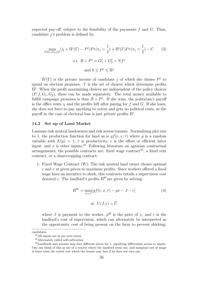
Candidate j’s problem is defined by:

maxP,G1,G2,f,Γ

(χ+ Πj(Γ)− P j)Pr(πj >1

2) + Πj(Γ)Pr(πj <

1

2)− C (1)

s.t. R + P j = Gj1 +Gj

2 +Nf j

and 0 ≤ P j ≤ Πj

C is the cost of running. Winner recieves non-pecuniary rents from

office, χ, and central government funds R, which is used to pay for G1, G2

and f conditional on winning.15 Πj(Γ) is the private income of candidate j

of which she choses P j to spend on election promises. Γ is the set of choices

which determine profits Πj. The total money available to fulfill campaign

promises is thus R+ P j. If she wins, the politician’s payoff is the office rents

χ and the profits left after paying for f and G. If she loses, she does not have

to pay anything to voters and gets no political rents, so the payoff in the case

14Details of the electoral market are based closely on Persoon and Tabellini (2008) and reservedfor the appendix

15χ is interpreted as the bureaucratic connections (the benefits are large but not immediate)available to an office holder as opposed to monetary benefits that could be used in combinationwith R to fulfill promises. While it is possible to use bureaucratic connections to benefit voters,e.g. through offering public sector employment (Robinson and Verdier 2002), I abstract from thatdimension of office rents and restrict the ability of the politician from using χ towards voters;this makes the problem tractable, although including this ability will not change results in anysubstantial way.

11

of electoral loss is just private income, Πj. Candidates maximize expected

pay-off, subject to the feasibility of the payments f and G.

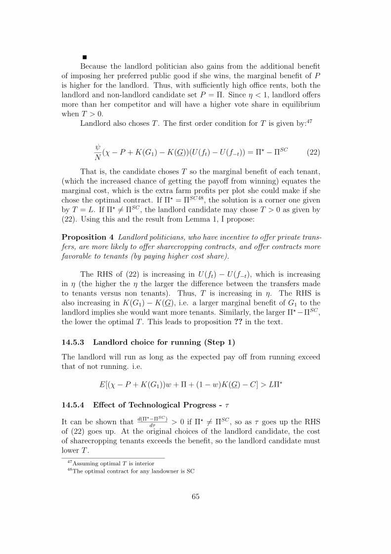
Following the literature on contractual choice in agriculture I consider

three kinds of rental contracts in a context with risk neutral landowners and

risk averse tenants (see appendix for details): fixed wage contract16, a fixed

rent contract, or a sharecropping contract.

1. Fixed Wage Contract (W): Land owner choses optimal inputs, including

labor at a fixed wage, to maximize profits. Landlord pays a monitoring

cost to prevent workers from shirking.

2. Fixed Rent Contract (R): Tenant farms land and pays a fixed rent.

Tenant has incentives to supply optimal inputs, but also assumes all the

risk; if uncertainty is high the rent in an incentive compatible contract

may be too low.

3. Sharecropping Contract (SC): Tenants and landlords share the output

and input costs. This contract is given by (α, β) where α is the output

share and β is the cost share of the tenant. Tenant supplies the inputs;

since the tenant consumes only a fraction of the output, he bears less

risk and has less incentive to exert the optimal inputs.17

The contractual literature studies the conditions under which any of the above

contracts may be optimal (Cheung 1969, Eswaran and Kotwal 1985, Stiglitz

1974). The tradeoffs between incentives, monitoring costs and risk sharing

can lead to one contractual arrangement dominating the other.In general,18

1. If monitoring is costly and tenants are risk averse, landlord prefers share-cropping, SC.

2. If monitoring is costly, but risk aversion is low, the landlord prefers fixedrent, R.

3. If monitoring is cheap, landlord choses wage contract, W.

At any level of land productivity τ , there is an optimal contract which yields

profits Π?:

16Alternately called self-cultivation.17I assume away the monitoring cost in the sharecropping case, or analogously assume that it is

cheaper to monitor the sharecropper relative to the wage worker; this will be the case given thatthe sharecropper is payed partly in terms of the output and his incentives to shirk are thus lower.

18See appendix and relevant literature (Eswaran and Kotwal 1985, Stiglitz 1974)

12

Π?(τ) = max{ΠW (τ),ΠSC(τ),ΠF (τ)}

ΠW , ΠR and ΠSC are the maximized profits from the wage contracts,

fixed rent contracts and sharecropping contract, respectively, for a unit plot

(detailed in the appendix). For a landlord with total land L, the total profits

are given by LΠ?. For simplicity I assume homogeneous plots, the optimal

contract is one of the three, and is used to farm all plots by a profit maxi-

mizing landowner. All the intuitions follow through if the assumption is not

imposed.19

The timing of the model is as follows:

1. Landlord choses whether or not to run

2. If running, landlord choses (f,G1, G2, P ) and tenure contract; competingcandidate choses (f,G1, G2, P )

3. If not running, landlord only makes the contract decision for farming;candidates chose (f,G1, G2, P )

4. Election happens

5. Production happens

6. Winner delivers promises, payoffs are realized

I consider two cases: 1) Case 1: Baseline case where two non-landlords com-

pete. 2) Case 2: I allow landlord to run in election. Case 2 represents an

environment with a landowning oligarchy tht can employ landless or small-

holder tenants. As argued above, the members of the oligarchy act as a single

entity, which I will refer to as the landlord candidate in case 2. I assume log

functional form for U(f) and H(G) to get closed form expression for the policy

platforms. I am interested in analyzing how the policy platform and electoral

outcome is different in these cases; and also how these change in response to

shifts in land productivity τ . Before solving the electoral equilibrium, I show

how landowners can make private transfers to sharecropping tenants.

19With heterogeneous plots, the choice for contract will not be discreet. Instead, the landlordwill chose the share of her land to cultivate under each type of contract. In other words, foreach level of τ the landlord will chose the optimal (T ∗, F ∗) to maximize profits given by Π?(τ) =maxT,F{(L− T − F )ΠW (τ) + TΠSC(τ) + FΠF (τ)}.

13

3.2 Landlord can make electoral transfers to sharecroppers cheaply

Suppose a candidate, who owns land, wants to offer a private transfer to a

voter who is a sharecropping tenant. She can offer a direct lump-sum transfer

γε or alternately offer to lower the tenant’s cost share by βε, such that it is

monetarily equivalent to γε. However, lowering the cost share induces the ten-

ant to apply higher inputs and effort on the farm, which is partly internalised

by the landlord who shares the output. I show that:

Lemma 1 It will be cheaper to lower cost share of the tenant than offering a

lump sum transfer if ex-post the landlord would want the tenant to apply more

input.

This will be true if the landlord’s optimal application of inputs is higher

than what the tenant provides. By incentivising the tenant to supply more

inputs without increasing the risk borne by him, the net cost borne by a

landlord is lower when she makes an electoral transfer to a sharecropping

tenant through a more favorable contract than through a direct monetary

transfer. 20

3.3 Equilibrium

I solve by backward induction. Case 1 is symmetric; in equilibrium (ommiting

candidate superscript), G1 = G2 = G = R+P3

and f = GN

. Both candidates

have the same platform and winning probability is equal to one half in expec-

tation.

In Case 2, I denote transfers specific to tenants by ft and to non-tenants,

f−t. Denote the mass of sharecroppers by T , which the landlord choses.21

Additionally, the landlord’s payoff consists of direct utility from G1, which

she choses directly if elected and is given by K(G1). In the case of a land

owner with land L, the private pay-off is given by LΠcontract +K(G1), where

LΠcontract are total farm profits depending on the choice of contract and K

represents the land owners private benefit function from G1.22

20A decrease in the cost share can be equivalently thought of as an increase in the output shareof the tenant; however in the data the output share is traditionally fixed at one half. Hence, Iconduct the analysis in terms of the cost share.

21T = L if Π∗ = ΠSC . Given that sharecropping allows landlord to make transfers efficiently,the landlord may chose to have T > 0 plots under sharecropping, even when sharecropping is notthe optimal contract.

22See appendix for the landlord politicians problem.

14

Solving the landlord candidates problem in this case and using the result

from Lemma 1, we have the following propositions:

Proposition 1 If landlord runs in the election:

(a) Landlord selects policies such that G1 > G2 and G2 < G2 = G, i.e.

she over provides her preferred public good.

If T > 0 ,

(b) Landlord offers higher private transfers to tenants, ft > f−t. Thus

at any level of ideological preference, a tenant is more likely to vote for the

landlord candidate relative to another voter with the same ideological prefer-

ence.

(c) The landlord’s vote share and probability of winning exceeds the com-

petitor’s when T > 0, all else equal.

Proposition 2 When sharecropping is optimal the landlord sets T = L. Oth-

erwise, the landlord candidate sets 0 < T ≤ L as long as Π? − ΠSC is small.

In this case, T is larger if:

(a) η is large (b) dKdG1

is large (c) Π? − ΠSC is small.

When Π? − ΠSC is large T = 0

The competitor must set ft = f−t = f , G1 = G2 = G, since transfers to

tenants and to non-tenants are equally costly for winning votes, and so are

G1 and G2. The landlord competitor, on the other hand, values G1 relatively

higher compared to G2, and thus spends more on it. Additionally, tenants’

votes are cheaper relative to those of non-tenant voters, leading the land-

lord to accumulate greater vote-share from the tenant-voters. The incentives

for hiring sharecropper are higher the larger the electoral benefits of having

sharecroppers, and the lower the efficiency cost of sharecropping.

3.3.1 Effect of Technological Progress - τ

It can be shown that ΠSC is lower relative to ΠF and ΠW with technological

change (Eswaran and Kotwal 1985, Stiglitz 1974, Bardhan and Srinivasan

1971). In other words technological change causes a shift away from share

tenancy to either fixed rent or to fixed wage contracts, depending upon the

type of technological change. Labor augmenting technical change increases

the capital to effective labor ratio making supervision relatively less costly,

leading to wage contracts. On the other hand a land augmenting technological

15

change increases the effective labor per acre and the need to provide greater

incentives, shifting the optimal contract to fixed rent. A formal argument

showing the effect of technological change on the optimal contract is offered

in the appendix.

What does the shift in optimal agricultural contract imply for the polit-

ical economy? It can be shown that: d(Π?−ΠSC)dτ

> 0 if Π? 6= ΠSC , hence:

Proposition 3 A rise in τ that shifts the optimal contract away from share-

cropping will cause the landlord candidate to lower T

The intuition is that as land productivity increases, it is increasing costly

to have sharecropping tenants on one’s land. Moreover, profits are higher

regardless of the contact, so the landlord doesn’t need tenants any more to

increase her vote share. So landlord farms more of her land under the optimal

contract (wage or fixed rent).

The overall platform of the landlord candidate is also dependent on the

level of productivity τ . When τ is small, landlords profits are small relative to

χ, so landlord sets P = Π. T is high, so there is a large fraction of voters who

vote for the landlord, who then has higher winning probability. As τ increases,

there is a direct income effect due to higher overall profits, so electoral offers

are higher. There is also an opposing indirect effect due to the lower number

of tenants. Offering private transfer is costlier, causing landlords electoral

offers to be lower.

Suppose τ rises enough that it is optimal to set T = 0, the landlord

will still run as long as the office rents χ and marginal benefit of G1 is high.

The landlords winning advantage will no longer exist and her vote share and

winning probability will be lower. In general, as productivity shifts up, the

landlords electoral incentives become weaker, all else equal.

3.4 Testable Predictions

The following predictions are testable:

1. Landlord politicians, who have incentives to offer private transfers,

offer more sharecropping contracts, and offer contracts more favorable to ten-

ants (by paying a higher share of input costs)

2(a). Technical change in agriculture lowers sharecropping, if the cost

of monitoring labor remain stable

16

If technical change lowers (raises) landowners probability of win, then

on average:

(b) Electoral competition is better (worse)

(c) Public goods favored by landlords are lower (higher) relative to other

public goods

4 Empirical Strategy

4.1 Landlord Politicians and Agricultural Tenancy Contracts -Testable Prediction 1

Testable prediction 1 states that a landlord with political incentives is more

likely to have sharecropping tenants. Table 2 indicate landlord politicians are

more likely to have sharecropping tenants, have more land as well as more

tenants. These differences are far from causal; there may be unobservable

differences in the land quality across different landowners. The tenants of

landlord politicians may also be systematically different from other tenants

leading to differences in the contract terms they face. To best disentangle the

effect of political incentives of the landlord, one should compare the contracts

between the same landlord-tenant pair when the landlord has successfully

participated in an election.

To identify the effect of a landlord-politician, I use the introduction of

an election after a military regime as a natural experiment in combination

with a panel data-set (Pakistan Rural Household Survey). The first round of

the data is from the 2000-01 agricultural season, when the country was under

a military regime after a coup 1999; the following round is from 2003-04, after

a general election had occurred in 2002.23 Thus, in the pre-election round

there are no active and directly elected politicians while in the post-election

round tenants in the survey indicate if their landlord is a winning politician.

I use this data to deduce if the election incentives induces politically involved

landlords to offer better contracts to gain tenants’ electoral support.

Ideally, I want to compare contracts on the same plot of land leased

out by a landlord in a year she faces electoral incentives relative to when

she doesn’t - in other words compare the same plot before and after the

introduction of the election. However, I only have a household-level panel,

23The previous general election was held in 1997, however, the government was dissolved andreplaced by a military government within a year.

17

but not plot-level. I run the following plot-level specification.

Spec 1: yi,j,p,t = γ1PlothasPoliticianLL PostElectioni,j,p,t +

γ2PostElectiont + γ3ηp + γ4σj + γ5ςi,j + κi + εi,j,p,t,

where yi,j,p,t is the contractual arrangement for tenant i, landlord j,

plot p in year t, PlothasPoliticianLL PostElectioni,j,p equals 1 for plots in

the PostElection round where the landlord is an elected politician. κi is a

household fixed effect. I also control for plot characteristics ηp, characteristics

of the landlord σj, as well as other landlord-tenant level controls ςi,j, including

whether they belong to the same caste and the length of contract between

them. The PostElection dummy accounts for the fact that election years

are systematically different from other years (Khemani 2004). The outcome

variables include the type of contract (fixed rent versus sharecropping), and

within the sharecropped plots, the landlord’s output and input cost-share

(seed, fertilizer, ground water and harvesting costs). All errors are clustered

at the household level. The survey visits households, who may be tenants

or landlords; in other words each observation represents a plot, which may

be leased in by the responding household (i.e. household is the tenant) or

leased out by the responding household (i.e. household is the landlord). I run

the regression using only leased in plots, as well as pooling the leased-in and

leased-out plots. In the former case the household fixed effect is analogous

to a tenant fixed effect. Essentially, this specification allows me to compare

a plot where landlord is a winning politician to all other plots of the same

tenant.

The above specification assumes tenants do not switch to renting plots

from new (and significantly different) land-owners between the rounds. In the

data, the average length of relationship of a landlord-tenant pair is 8 years, so

this assumption is not entirely catastrophic. If this assumption was univer-

sally true, then just having the tenant fixed effect controls for any systematic

differences between politically involved landlords and the quality of their land

relative to other landowners. However, to ensure the above estimation is not

biased by tenants switching plots and to control for these systematic differ-

ences I run another plot-level specification. Tenants also report if their land-

lord is a politician in the pre-election round, which implies the landlord was

elected in the previous election, but is not in currently office due to the coup.

Provided these politicians from the last election did not expect re-elections

18

immediately after the coup, they have no incentives to offer any additional

benefit to tenants. This incentive is present in the latter round just after

the election; we expect landlord politicians to have different contracts relative

to other landlords only in the post-election round. This specification is as

follows:

Spec 2: yi,j,p,t = β1PlothasPoliticianLL PreElectioni,j,p,t +

β2PlothasPoliticianLL PostElectioni,j,p,t + β3PostElectiont + β4ηp +

β5σj + β6ςi,j + κi + εi,j,p,t

PlothasPoliticianLL PostElectioni,j,p,t is the same as before. PlothasPoliticianLL PreElectioni,j,p,t

is a dummy that equals 1 for a leased plot where landlord is a politician. I

treat landlord politician in the previous round as a control group. It controls

for differences due to the fact that the plot is owned and leased out by politi-

cally involved landowners, who are indeed different for a variety of reasons. β2

measures the differences in the contractual terms offered when the landlord is

a politician and has an incentive for making electorally motivated transfers.

To further check whether some contracts are significantly different from

others regardless of the election, I create a dummy that equals 1 for a tenant

in the pre-election round if he reports having a politician landlord after the

election. The specification and results are provided in the appendix. I also run

placebo regressions using landlords who hold an influential but non-political

position. Non-political positions include those for which the landlord does not

have to be directly elected, e.g. a religious leader or a village council head.

4.2 Technological Change and Tenancy and Electoral Outcomes -Testable Predictions 2(a)-(c)

Testable predictions 2(a)-(c) state that shifts in land productivity should shift

tenure contracts, as well as electoral and policy outcomes in areas where land-

lords are initially dominant. A permanent shift in productivity will affect

landowners incomes as well as their incentives for sharecropping tenancy;

consequently, it will shift landowners participation in politics, and the pub-

lic goods which are provided (direction of effect is ambiguous depending on

whether productivity shift increases or decreases landlords’ political participa-

tion). I test the effect of technological change using data on voting outcomes

and politicians’ assets from general elections between 2002-2013, and using

19

data on allocation of public goods.24 I need a measure of agricultural pro-

ductivity as well as a measure of initial landlord dominance, which I describe

below.

4.2.1 Constructing a measure of Exogenous Technological Change

Agricultural yields and electoral outcomes are likely to affect each other, and

are likely affected by underlying human capital and institutional character-

istics of a region. To deal with the endogeneity of agricultural productiv-

ity, I construct a measure of exogenous productivity change using variations

in suitability and availability of high-yielding variety (HYV) seeds. Foster

and Rosenzweig (1996), among others, note two important features of pro-

ductivity gains from high yielding varieties making this technology plausibly

exogenous. First, the HYV seeds were originally imported from outside the

countries which adopted them. Secondly, the profitability of the improved

seeds is heterogeneous across the space because of (exogenous) differentials in

local soil and climate conditions.

I exploit spatial variation in HYV suitability and time variation in the

availability of HYV to construct a measure of productivity shock due to HYV

in area j and year t, for crop c. SuitHjc is suitability for crop c in area

j with high technology (mechanized inputs, fertilizer and irrigation), while

SuitLjc is the same with low technology (traditional inputs and rain fed).

Since HYV seeds are most profitable with mechanized inputs and irrigation

(Shiva1991), the difference between the two suitability indices, SuitDiffjc

captures the extent to which area j will gain from the HYV technology.

HY Vcpt is the total amount of improved seeds available in a province in any

year for any crop.25 The interaction of the difference in suitability and the

HYV, SuitDiffcj ×HY Vcpt, gives a time and area varying measure of shock

to agricultural productivity (See Figures 1-2).

Table 10 shows that constructed measure is significantly correlated with

the actual yields by crop, allowing me to use it as a proxy for shifts in agricul-

tural productivity resulting from technological innovations in seeds. For any

district I use SuitDiffcj×HY Vcpt, where c is most widely grown crop in that

24The household data set above does not cover all districts of the country25Variation in HY Vcpt is driven by the availability of these seeds from the foreign producers in

any year, and is thus exogenous to any area-specific characteristics which may lead to lower orhigher HYV adoption.

20

district in 1980 to measure technological change at region-time level.26 Since

electoral outcomes and the productivity instrument is at constituency level,

but actual yields are not available at constituency level, I run reduced form

regressions instead of 2SLS.27

4.2.2 Constructing a measure of Historic Landlord Dominance

Using the colonial land estate data mentioned in the Data section, I construct

a dummy variable LLDominated for each sub-district which equals 1 if a large

colonial estate was assigned to a dominant landlord. These include grants that

were significant in size and described as notable estates, or the grantee has

been reported to be a notable ”jagirdar” in the colonial records. Detailed

records of land assignments is not available for all provinces - for some areas,

only the notable ”jagirdars” are listed. To maximize the data points and use

all the provinces, I use the non-continuous measure. Summary statistics in

Table 3 show that landlord politicians are more likely to be present in the areas

where LLDominated equals 1. The sharecropping rate and land concentration

is also high in these areas, and public goods are generally worse.

I confirm that landlord dominated and other areas are balanced along

observable historic characteristics like population density, land revenue per

acre and religious composition of population. In fact the historical accounts

suggest land assignments or ”jagirs” were granted by pre-colonial dynasties,

and were not likely to be driven by any specific agenda, other than to reward

loyal locals in different parts of the empire. It is also reassuring to note that

SuitDiffj is not systematically different across regions with and without

dominant landlords.

Using these measures, I estimate the equation:

yjt = β1 + β2SuitDiffj ×HY Vpt + β3SuitDiffj ×HY Vpt ×LL Dominantj + νj + µpt + εjt

where yjt is the outcome of interest in area j (constituency or district) and

year t and LL Dominant is the measure of landlord dominance.Technological

change measure SuitDiffjt × HY Vpt is at j, t level, thus I can include con-

stituency (or district) as well as province-year fixed effects, to account for

26By using the crop choice from an initial period (1980), I avoid confounding factors due toendogenous crop choice.

27The smallest level for which I have actual yields is district; I estimate and report the 2SLSregressions using predicted district-level yields for the district-level regressions.

21

time-invariant geographic heterogeneity and province specific time trends, re-

spectively. I examine the following outcomes as function of the interaction of

agricultural productivity and landlord dominance: the rate of sharecropping

and owner cultivation (district level), politician’s land-holding status and size

of land held, measures of electoral competition (constituency level), and the

types of public goods provided (district level). The coefficient of interest is

β3; if higher agricultural productivity lowers landlords’ political participation,

we expect β3 to be negative when the dependent variable is an indicator for

landowning politician or if the dependent variable is an indicator for low elec-

toral competition. Similarly lower political participation by landlords also

implies that β3 will be negative for measures of landlord preferred public

goods.

I run robustness specifications with additional LLDominated×Y ear and

District× Y ear fixed effects to account for area specific differential trends in

agricultural tenure and electoral outcomes. Additionally, to account for the

income effect of increased productivity, I run the above specification replacing

SuitDiffjt×HY Vpt with rainfall as a proxy for income. SuitDiffjt×HY Vpt is

a measure of a permanent improvement in land productivity, which can shift

incentives for sharecropping. Rainfall measures, on the other hand, simply

capture variation in incomes of landlords and rural voters, but will not affect

the optimal agricultural contracts.

5 Data Sources and Description

I use two rounds of the Pakistan Rural Household Survey (PRHS 2000 and

PRHS 2003), comprising a panel of households, to study landlord politicians

and the contractual terms they offer. Landlord politicians are landowners

who are identified as a politician by the tenant, implying the landlord ran and

won in an election. Information is available at plot level - plot characteristics,

leasing status (self-cultivation versus sharecropping contract or a fixed rent

contract), contract terms, input/outputs and characteristics of the cultivating

households. If the responding household is a tenant, i.e. leasing in a plot,

information about the landlord is obtained and vice versa for leased out plots.

The data for agricultural land distribution, tenancy and crop areas and

yields, and HYV seeds is obtained from various issues of the Agricultural

Statistics of Pakistan (Government of Pakistan). These data are generally

22

at district level.28 The data for the politicians assets and voting outcomes at

electoral constituency level comes from the Election Commission of Pakistan.29

Districts contain several constituencies depending on the population density.

Each electoral constituency comprises of 120,000 voters on average. Due to a

bill in 2002, all office holders are required to declare all assets and liabilities.

I use only the politicians who have been elected by a direct election to the

Provincial Assemblies. This is the lowest level at which voters can elect their

representatives.

The historical data for compiling the estate grants comes from a variety

of sources including the province and district gazetteers and land settlement

reports, which were compiled by Government of India in late 19th-early 20th

centuries, and include information on ‘zamindars’ and ‘jagirdars’. Addition-

ally, an extensive list of aristocrats was maintained in ”The Punjab Chiefs”

(Griffin and Craik 1865), by the colonial authorities. This was used in com-

bination with district and province gazetteers and settlement reports to com-

pile the notable jagirs or land assignments by subdistrict level. The different

sources are used to verify that no significant ‘jagirdar’ is missed.

For constructing the measure of technological change I use the Global

Agro-Ecological Zones database (FAO), which provides suitability indices and

potential attainable yields for all crops by type of irrigation and input tech-

nology for a worldwide grid at a resolution of 9.25 x 9.25 km. These indices

depend on the climatic and agro ecological conditions of the area and are pro-

vided for different hypothetical levels of technology (high and low). In order

to match the FAO suitability data with electoral outcomes variables I super-

imposed each of the suitability maps (for both high and low technology) with

political maps of Pakistan reporting the constituency and district boundaries.

Next, I compute the average of the suitability values for all cells falling within

the boundaries of every constituency/district.

The data on public goods is drawn from the Pakistan Living Standards

Measurement Surveys (PSLM 2006, 2008, 2010); There are 2 separate elected

governments in this period. The PSLMs asks survey respondents about their

use and the availability and quality of public services; this is at district level.

28There are over a 100 districts at present; historically there were fewer districts and there arenumerous incidences of division of districts to form new ones

29Provincial Assemblies are analogous to State Legislatures in the U.S. and is the lowest level atwhich officials are democratically elected.

23

6 Results

The regression results in Tables 4 (and 7A) show that in the round after the

election, the landlords who are politicians are more likely to have tenants on

sharecropping contracts. This result is stable across the different specifications

and with a rigorous set of controls. A given tenant is 17 percentage points

more likely to have a sharecropping contract on the plot leased out by a

politician relative to all other leased plots of the tenant where the landowner

is a non-politician or when the regime is non-democratic. This is 21% higher

than average rate of sharecropping in the sample.

Next, I look within the sharecropped plots, to test if the contractual

terms change when the landlord has a political motive to do so (Table 5

and 8A). Positive and significant coefficient on the indicator for a landlord

politician implies that the landlord politicians offer to pay a greater share of

costs in the round after the election (The cost share of seeds is an exception).

On plots with an leased out by politicians, the landlord increases her offer

of ground-water cost-share by 27% and harvesting cost-share by about 45%.

There is no significant change in the share of output kept by the landlord. I

also examine the access to canal water, which is a strategic input and appears

to be central to village-level conflicts in the data. I find (Tables 6 and 9A)

that specifically on sharecropped plots, tenants of politicians are much likely

have access to canal irrigation. These results offer satisfactory support for the

predictions of the model. Indeed, politically motivated landowners seems to

rely on their access to land to fulfill clientelistic endeavors towards tenants

and landless farmers in their villages.

In section 7, I run robustness checks to rule out that there are no pre-

existing trends in the contract types or contractual terms. To rule out that the

effect of landlord politician on post-election terms in not simply an election

effect, I run a placebo regression using landlords who hold an ‘influential’ but

non-political position. I find no effects using these placebo indicators.

To test predictions 2(a)-(b), I use the specification described in section

4. If the technological change due to HYV seeds increases per acre yield

relative to monitoring costs, we expect landowners to shift away from share-

cropping contracts towards self cultivation using hired wage labor. Figure 3

shows the trend in the distribution of sharecropping rates across the districts

of Pakistan over five decades; there has been drastic fall in the rate of ten-

24

ancy. The regression results in Table 11 show that the productivity increase

due to HYVs indeed caused the rate of sharecropping to go down, and the

rate of self-cultivation to go up. A 0.5 ton/ha increase in yield30 lowers the

rate of sharecropping by 28%; these effects are indeed large and significant.

The relatively stable distribution of land ownership over this time (Figure 4)

indicates that changes in the distribution of land ownership can only be partly

responsible for shifts in the tenancy rates.

The next set of regressions (Table 12-13) looks at the landholdings of

the elected members of the Provincial Assemblies and the degree of electoral

competition in these elections. technological change within a landlord domi-

nated constituency leads to lower likelihood that the winning politician owns

agricultural land. An increase in productivity corresponding to a 0.5 ton/ha

increase in actual yield lowers the winning probability of a landowner in ar-

eas with historic land assignments by 13 percentage points. I also use the

holdings-size and number of agricultural properties of the winning politician

as the dependent variable; the effect is again negative.

Table 13 shows that lower landlord winning probability corresponds to

improved electoral competition. This is shown using a Herfendhal index for

winmargin and alternately a categorical variable for low competition, which

is 1 when the win-margin is below the 25th percentile. Using the actual win-

margin as the dependent variable or shifting the cut-off to classify Lowcomp

yields similar results (see appendix Table A5). A productivity shock amount-

ing 0.5 ton/ha increase in yield lowers the likelihood of an uncompetitive

election by 18 percentage points in the areas with historic land assignments.

In more stringent specifications, I add LLDominated×Y ear andDistrict×Y ear fixed effects. These results, explained in Section 7 provide reassurance

that results are not driven by differential trends in historically landlord domi-

nated areas or other alternate mechanisms. Similarly, using rainfall shocks as

proxy for income, I check that the rising incomes due to the productivity shift

is not the mechanism that leads to the shift of political power and electoral

competition.

The outcome directly relevant to development is public goods; the agri-

cultural shock affects the identity of winning politicians, who in turn allocate

public goods. Thus, to estimate the impact of the exogenous technological

30The green revolution increased wheat yields up to three-fold; as Table 3 shows between 1965and 2002 the yields increased from 0.7 ton/ha to over 2.5 ton/ha.

25

shift on public goods, I use the SuitDiff × HY V measure from the year

preceding the last election before the public goods data was collected. By

doing so, I am able to capture the impact of the agricultural productivity

shock through its affect on the identity of elected politicians who determine

how public goods are allocated. The outcome I consider is the percentage of

respondents from any district that report an improvement in the availability

of a facility over the past year. Since I have different categories of public

goods, I also obtain a principal component of the different categories, and use

that as a dependent variable.

First I distinguish between the use of facilities across land-owning status

(Table 14). I would like to identify public goods which are specifically benefi-

cial to large landowners. I regress households’ self-reported frequent use of a

facility on an indicator for whether the household’s land holdings in the top

5th percentile. Landowners are more likely to use police stations and vet, and

less likely to use a basic health unit or family planning services. They are

neutral towards drinking water and roads. Moreover, as the literature about

targeting ”core voters” (Cox and McCubbins 1986) suggests that landlords

may target their voter base and provide more facilities in rural areas, I dis-

tinguish publicly provided facilities in rural or landlord-preferred areas from

those in urban areas.

Regression results are shown in Table 15-17. Firstly, Table 15 suggests

an improvement in basic health unit, family planning and drinking water ser-

vices, specifically in the landlord dominated areas, as a result of exogenous

technological change. The effect on other public goods isn’t precisely esti-

mated in the landlord dominant areas. However, the next set of results in

Table 16 helps unpack this by looking at the effect of the productivity shift

and resulting shift in political influence of landlords on public goods across

rural and urban areas. I add an additional interaction with a dummy for ru-

ral areas. For all public goods the coefficient for productivity interacted with

landlord dominance has the opposite signs for rural and urban areas. The

improvement in public goods is concentrated specifically in the urban areas.

Basic health unit, family planning are drinking water improve overall, but are

significantly better in urban relative to rural areas. The landlord preferred

public goods are overall lower in rural areas, and vet facilities are significantly

worse relative to urban areas. Road, a landlord-neutral good, improves in ur-

ban areas, but not in rural areas. This is suggestive evidence that traditional

26

politicians not only steered resources towards services which benefited farm-

ers directly, but favored rural areas in provision of all other services. A shift

in power towards the modern elite and away from the traditional rural elite

results in a shift of resources towards urban areas. The results thus speak to

the rural-urban inequality and the rural-urban migration, which is a strong

feature of developing economies.31

7 Robustness

To test the robustness of the results in Tables 4-6 I run placebo regression

using landlords who hold an influential but non-political position, or are large

landlords. Non-political positions include those for which the landlord does

not have to be directly elected, e.g. a religious leader or a village council

head. I find no effects using these placebo indicators. Additionally, including

a dummy for a non-political position of influence as a control in the my main

specifications does not alter the results. This gives assurance that the above

results are not just driven by the fact that the landlord is influential or has

large land holdings, but only that she has an incentive to transfer utility to

the tenant for gaining political support. I do find that very large landlords

are likely to change their contracts after the election. This aligns with the

idea that large landlords have a coalition and collude to offer clientelisticly

motivated contracts to tenants. Results are shown in appendix Table A2.

As a robustness check and to ensure there are no pre-trends, I can use

an earlier panel data set by the International Food Policy Research Institute

(IFPRI), which covers 12 rounds in the period from April, 1986 to September,

1989 in a sample of the same villages from the PRHS surveys. This time frame

is useful because it also contains a spell of non-democratic regime followed by a

general election in 1988. I do two sets of regressions to check for pre-trends in

the rate of sharecropping and in the availability of inputs from the landlord to

sharecropping tenants. In Figure 6 I plot the coefficient on each year dummy

from a household level regression of an indicator for sharecropping on year

dummies, household (tenant) fixed effects, and round and season fixed effects.

There are no specific trends in the rate of sharecropping or the inputs provided

by the landlord during the non-democratic regime; however as expected after

31These results are confirmed using another data set for rural pubic goods. Results available onrequest

27

the election in 1988, the rate of sharecropping as well as the landlords’ payment

for inputs spike up. I do not have information on the landlords political status

in this dataset and cannot test if the spike is indeed due to landlords’ political

transfers (as I do in the main regression using PRHS data above).

I argue that the results in Tables 12-13 are not driven by differential

growth path of areas which were historically different, other than through

the differential effects of variations in agricultural productivity. I can control

for differential trends specific to areas with the historic land assignments by

adding LLDominated × Y ear fixed effects. Results in columns 1-3 of Table

A3 shows that the effect of technological change in landlord dominated areas

is robust to controlling for trends specific to the landlord dominated areas

that were correlated with improvements in productivity.

There could still be alternate trends in some areas which coincided with

improvements in productivity. For example, technological change will increase

the marginal product of capital, plausibly causing the entry of capitalist elites

into politics. Similarly, rural-urban migration or a shift in agricultural wages

can lower the traditional landowner’s prominence relative to urban elites.

These mechanisms will also lead to lower likelihood of landowners’ success

in elections and improve electoral competition. For the results above to be

biased it would have to be the case that these trends operated differently

in landlord dominated areas. While, the province-year fixed effects in the

regression accounts for any province specific trends in the emergence of capi-

talists, rates of migration as well as other changes over time. To further test

the robustness of my results, I run a very stringent specification by adding

district-year fixed effects. The results in columns 4-6 of Table A3 estimate

the effect of differences in productivity in constituencies within the same dis-

trict and year. The coefficients are lower due to the strict controls but the

effect is robust. The increasingly rigorous specifications confirm that the lower

success of landowners in politics and improved electoral competition cannot

be entirely explained by alternate district specific trends like the differential

growth in the non-agricultural sector or differential rate of urbanization across

districts.

Lastly, the results maybe driven by the ”income effect” - as agricultural

productivity improves, voters are better-off and lead to differential electoral

outcomes by changing their voting behavior. To test the effect of improved

income of voted, I use rainfall shocks as an instrument for income. I run the

28

same specification, but the proxy for agricultural productivity is replaced by a

proxy for income. Rainfall will capture shocks to income, which are unrelated

to permanent improvement in agricultural productivity. Results are shown in

the appendix (Table A4) and highlight that the income effect is not entirely

responsible for the changes we see in response to exogenous improvement in

agricultural productivity. As expected, an overall income effect is present, but

there is no differential income effect in the landlord dominated areas. Thus

the electoral effect of improvements in agricultural productivity through the

cost of sharecropping to large landowners is robust and only operates in the

landlord dominated areas.

8 Concluding Remarks

The results support the view that initial asset distribution matters, and af-

fects growth as well as income and political inequality. Colonial institutions in

Pakistan induced the initial distribution of political power, whereby landown-

ing elites were able to capture and retain political influence and impress upon

policy outcomes. The results show one way in which traditional landowning

elites are able to perpetuate their political influence by gaining the loyalty of

sharecropping tenants. The process of development undermines the elites’ in-

fluence - agricultural technological change lowers sharecropping and effectively

alters the nature of paternalistic institutions in agriculture. This has implica-

tions for landlords’ success in politics and the resulting electoral competition

and public goods allocation.

I find that landed elites, when in power, provide facilities that benefit

farmers and their voter base. The shift in political power away from the tra-

ditional landed elites and toward the modern elite also results in a shift of

resources; resources are transferred away from the goods which benefit rural

voters, and in favor of urban voters. These results speak to rural-urban in-

equality and rural-urban migration, which is a common feature of developing

economies. A direct examination of the differential development of rural and

urban areas in response to the shift in elites’ identity and incentives can shed

more light on this finding. Moreover, by following individual landlord politi-

cians over time, we can better understand the changes in landlords’ incentives

for participation in politics in response to changes in agricultural productivity

as well as track partisan change in Pakistani politics.

29

The paper corroborates the evidence in favor of historical institutional

persistence and examines the vastly studied question of paternalism in tra-

ditional societies in a theoretic and empirical framework. The questions ad-

dressed in the paper have been long-standing themes in the study of polit-

ical economy, but rarely examined with data. Using more data from other

instances with traditional landowner dominance can provide relevance and

generalizability of the findings in other contexts.

30

References

Acemoglu, D., S. Johnson, and J. A. Robinson 2001: The Colonial Originsof Comparative Development: An Empirical Investigation, AmericanEconomic Review, 91, 1369-1401

Acemoglu, D., S. Johnson, and J. A. Robinson 2002: Reversal of Fortune:Geography and Institutions in the Making of the Modern World IncomeDistribution, Quarterly Journal of Economics, 117, 1231-1294.

Acemoglu, D., Johnson, S., Robinson, J. and Yared, P. 2008. ”Incomeand Democracy.” American Economic Review, 98(3): 808-42

Acemoglu, D., Reed, T., and Robinson, J. A. (2014). Chiefs: Elite Controlof Civil Society and Economic Development in Sierra Leone. Forthcom-ing in the Journal of Political Economy, 122.

Alston, L. J., and Ferrie, J. P. (1999). Southern Paternalism and theAmerican Welfare State: Economics, Politics, and Institutions in theSouth, 1865-1965 (p. 119). Cambridge: Cambridge University Press.

Baland, J. M., and Robinson, J. A. (2008). Land and Power: Theory andEvidence from Chile. American Economic Review 98: 173765.

Baland, J. M., and Robinson, J. A. (2012). The political value of land:political reform and land prices in Chile. American Journal of PoliticalScience, 56(3), 601-619.

Banerjee, A. V., and Iyer, L. (2002). History, institutions and economicperformance: the legacy of colonial land tenure systems in India.

Banerjee, A. V., and Iyer, L. (2008). Colonial land tenure, electoral com-petition and public goods in India. Harvard Business School.

Banfield, E. C. (1967). The moral basis of a backward society. New York,NY

Bell, C., and Srinivasan, T. N. (1989). Interlinked transactions in ruralmarkets: An empirical study of Andhra Pradesh, Bihar and Punjab.Oxford Bulletin of Economics and Statistics, 51(1), 73-83.

Berdegue, J. A., and Fuentealba, R. (2011). Latin America: The state ofsmallholders in agriculture. In Paper presented at the IFAD Conferenceon New Directions for Smallholder Agriculture (Vol. 24, p. 25).

Braverman, A., and Stiglitz, J. E. (1982). Sharecropping and the inter-linking of agrarian markets. The American Economic Review, 695-715.

31

Braverman, A., and Stiglitz, J. E. (1986). Cost-sharing arrangements un-der sharecropping: moral hazard, incentive flexibility, and risk. Amer-ican Journal of Agricultural Economics, 68(3), 642-652.

Braverman, A., and Srinivasan, T. N. (1981). Credit and sharecropping inagrarian societies. Journal of Development Economics, 9(3), 289-312.

Brenner, R. (1976). Agrarian class structure and economic developmentin pre-industrial Europe. Past and present, 30-75.

Brockett, C. D. (1992). Measuring political violence and land inequalityin Central America. American Political Science Review, 86(01), 169-176.

Boone, C. (1994) States and ruling classes in postcolonial Africa: theenduring contradictions of power. J. Migdal, A. Kohli, V. Shue (Eds.),State power and social forces: domination and transformation in theThird World, Cambridge University Press, New York , pp. 108139

Chanock, M. (1985) Law, custom, and social order: The colonial experi-ence in Malawi and Zambia. Cambridge University Press, New York

Cox, G. W., and McCubbins, M. D. (1986). Electoral politics as a redis-tributive game. Journal of Politics, 48(2), 370-389.

Dell, M. (2010). The persistent effects of Peru’s mining mita. Economet-rica, 78(6), 1863-1903.

Dixit, A., and Londregan, J. (1996). The determinants of success of spe-cial interests in redistributive politics. Journal of politics, 58, 1132-1155.

Economist 2013 Gone with the wind. May 18.

Engerman, S. L., and Sokoloff, K. L. (2005). Colonialism, inequality,and long-run paths of development (No. w11057). National Bureau ofEconomic Research.

Eswaran, M., and Kotwal, A. (1985). A theory of contractual structurein agriculture. The American Economic Review, 352-367.

Galor, O., Moav, O., and Vollrath, D. (2003). Land inequality and theorigin of divergence and overtaking in the growth process: theory andevidence (No. 2003-04). Working Paper, Brown University, Departmentof Economics.

Galor, O., Moav, O., and Vollrath, D. (2009). Inequality in landowner-ship, the emergence of human-capital promoting institutions, and thegreat divergence. The Review of economic studies, 76(1), 143-179.

32

Gazdar, H. (2009). The Fourth Round, And Why They Fight On: AnEssay on the History of Land and Reform in Pakistan. PANOS SouthAsia, Collective for Social Science Research, Karachi.

Glaeser, E., and A. Shleifer 2002: Legal Origins, Quarterly Journal ofEconomics, 117, 1193-1230

Grabowski, R. (2002). East Asia, land reform and economic development.Canadian Journal of Development Studies. 23(1), 105-126.

Griffin L. H. and Craik H. (1865). The Panjab Chiefs. Sang-e-Meel Pub-lication (repiublished 1993). Punjab (India)

Hussain, A. (1979). Elite politics in an ideological state: the case ofPakistan. Folkestone: Dawson.

Joshi, P. C. (1970). Land Reform in India and Pakistan. Economic andPolitical Weekly, A145-A152.

Kaplan, S. (2013). Power and Politics in Pakistan. Expert Analysis: Nor-wegian Peacebuilding Resource Centre, April.

Keefer, P., and Vlaicu, R. (2002). Clientelism, credibility and democracy.World Bank: Washington, DC Processed.

Keefer, P. (2007). Clientelism, credibility, and the policy choices of youngdemocracies. American journal of political science, 51(4), 804-821.

Khan, M. (1995). State Failure in Weak States: A Critique of New Insti-tutional Economics. In; Harris, J., Hunter, J. and Lewis, C. Eds. 1995.The New Institutional Economics and Third World Development. Lon-don: Routledge. pp 71-87.

Khan, M. (2010). Political Settlements and the Governance of Growth-Enhancing Institutions. Draft Paper in Research Paper Series onGrowth-Enhancing Governance. Faculty of Law and Social Sciences,School of African and Oriental Studies (SOAS).

Khemani, S. (2004). Political cycles in a developing economy: effectof elections in the Indian states. Journal of Development Economics,73(1), 125-154.

La Porta, R., Lopez-de-Silanes, F., and Shleifer, A. (2008). The economicconsequences of legal origins. Journal of Economic Literature, 46(2),285-332.

Logan, C. (2011). The Roots of Resilience: Exploring Popular Supportfor African Traditional Authorities. Working Paper no. 128, AFRO-barometer, Michigan State Univ.

33

Mamdani, M. (1996) Citizen and subject. Princeton University Press,Princeton, NJ

Martinez-Bravo, M., Qian, N., and Yao, Y. (2011). Do local elections innon-democracies increase accountability? Evidence from rural China(No. w16948). National Bureau of Economic Research.

Mason, T. D. (1986). Land reform and the breakdown of clientelist poli-tics in El Salvador. Comparative Political Studies, 18(4), 487-516.

Medina, L. F., and Stokes, S. (2002, August). Clientelism as politicalmonopoly. In the 2002 Annual Meetings of the American Political Sci-ence Association Conference. Boston. August (Vol. 29).

Merry, S.E. (1991) Law and colonialism. Law and Society Review, 25 (4),pp. 889922

Migdal, J. (1988) Strong societies and weak states: statesociety relationsand state capabilities in the Third World. Princeton University Press,Princeton, NJ (1988)

Nunn, N. (2009). The importance of history for economic development(No. w14899). National Bureau of Economic Research.

Piliavsky, A. (2014). Patronage as the Politics of South Asia. Cambridge:Cambridge University Press.

Persson, T., and Tabellini, G. E. (2002). Political economics: explainingeconomic policy. MIT press.

Powell, J. D. (1970). Peasant society and clientelist politics. The Ameri-can Political Science Review, 411-425.

Rashid, S. M. (1985). Land Reforms in Pakistan. Social Scientist, 44-52.

Robinson, J. A., and Verdierz, T. (2003). The Political Economy of Clien-telism.

Roberts, R. and Mann, K. (1991) Law in colonial Africa. K. Mann, R.Roberts (Eds.), Law in Colonial Africa, Heinemann, Portsmouth, NH,pp. 358

Scott, J. C. and B. J. Kerkvliet (1976) How traditional rural patrons loselegitimacy: a theory with special reference in Southeast Asia, pp. 439-458 in S. W. Schmidt, L. Guasti, C. H. Lande, and J. C. Scott (eds.)Friends, Followers and Factions: A Reader in Political Clientelism.Berkeley: Univ. of California Press.

34

Stiglitz, J. E. (1974). Incentives and risk sharing in sharecropping. TheReview of Economic Studies, 219-255.

Time 2008. Landowner Power in Pakistan Election by Baker, A., andBhutto, M. February 13.

Times of Karachi 2011 Feudalism in Pakistan. January 1.

Vicente, P. C., and Wantchekon, L. (2009). Clientelism and vote buying:lessons from field experiments in African elections. Oxford Review ofEconomic Policy, 25(2), 292-305.

Zaidi, S. A. (2014). Rethinking Pakistan’s Political Economy: Class,State, Power and Transition. Economic and Political Weekly, 49 (5).pp. 47-57.

35

9 Figures

Figure 1: FAO Suitability for Wheat: High Input Level and Irrigation (Left),Low Input Level and No Irrigation (Right)

Figure 2: HYV Penetration across Years and Crops for Different Provinces0

.51

1.5

20

.51

1.5

2

05

1015

05

1015

1970 1980 1990 2000 2010 1970 1980 1990 2000 2010

BALUCHISTAN N.W.F.P

PUNJAB SINDH

Wheat Cotton Maize Rice

Impr

oved

Var

ietie

s of

See

ds (p

er h

ecta

r)

year

Graphs by province

36

Figure 3: Distribution of Sharecropping Rate (percent of area under share-cropping) across Districts

0.0

2.0

4.0

6D

ensi

ty

0 20 40 60 80Perc. of Total Area under Sharecropping (%)

1960 1972 1980 1990 2000 2010

Source: Relevant Annual Census of Agriculture

Figure 4: Distribution of Land Concentration across Districts

0.0

1.0

2.0

3.0

4D

ensi

ty

20 40 60 80Land Concentration Index

1972 1980 2000 2010

Note: The Land Concentration index is calculated as:(% of land with largeholders + % of land with smallholders/average size with smallholder)Source: Relevant Annual Census of Agriculture

37

Figure 5: The Historic ’Jagir’ Districts (Left) and Land Concentration (Right)

Notes: The left panel shows the districts coded as estate==1. The right panel shows the landconcentration index (Brockett 1992) using holdings data from 1972 agricultural census. Darkerareas represent high values of land concentration.

Figure 6: Pre-trends in Rate of Sharecropping (Left) and Inputs provided byLandlord in Sharecropping Contracts (Right)

-200

020

040

060

0

1986 1987 1988 1989

Election Year

-.04

-.02

0.0

2.0

4.0

6

1986 1987 1988 1989

Election Year

Notes: The left panel shows the coefficient on each year dummy from a regression of tenanthouseholds, regressing whether the household is a sharecropper as a function of household, round,season and year fixed effects. The right panel shows the coefficient on year dummies from the sameregression with the value of inout provided by landlord as the explanatory variable.

38

10 Summary Statistics Tables

Table 1A: Summary Statistics: Data for Testing Prediction 1

Self-cultivated Sharecropped Leased on Fix RentPlot area (kanals) 39.55 35.82 49.60

(53.84) (29.74) (102.6)

Irrigated 0.662 0.927 0.744(0.473) (0.261) (0.437)

Plot Yield (Rs/kanal) 1420.9 1288.3 1253.6(18690.8) (4368.7) (4196.0)

% area under wheat 0.510 0.390 0.636(0.362) (0.396) (0.370)

% area under rice 0.255 0.448 0.161(0.377) (0.428) (0.336)

% area under maize 0.0281 0.00714 0.0203(0.134) (0.0653) (0.112)

% area under cotton 0.195 0.169 0.418(0.328) (0.324) (0.437)

% area under sugarcane 0.0970 0.126 0.0826(0.304) (0.338) (0.236)

Number of Plots 1620 846 188

39

Table 1B: Summary Statistics: Data for Testing Prediction 1

LL is not Politician LL is PoliticianPlot is sharecropped 0.645 0.903

(0.479) (0.301)

Plot area (kanals) 57.06 25.29(103.0) (18.46)

Irrigated 0.847 0.935(0.360) (0.250)

Landlord Holding (kanals) 626.4 17016.8(1646.6) (23724.1)

Tenant Holding (kanals) 20.35 6(70.32) (20.48)

Plot Yield (Rs/kanal) 983.7 895.8(2528.3) (592.6)

Total tenants under the landlord 5.939 35.19(11.94) (28.79)

LL's Output share for sharecropped plots 52.62 49.39(13.25) (3.213)

LL's cost share for Harvesting costs 35.84 33.33(30.86) (24.02)

LL's cost share for Fertilizer costs 50.29 41.07(18.06) (18.28)

Number of Plots 960 74

40

Table 2: Summary Statistics: Data for Testing Prediction 2(a)-(c)

Estate=0 Estate=1 Difference Unit Source ObservationsAgriculture Perc. under sharecropping 23.2 31 7.8*** District Ag. Census 225

(17.0) (18.5)Land Concentration 39.0 44.8 5.8 District Ag. Census 47

(12.3) (11.2)Suitability Diff 2.00 2.22 0.22 9.25 × 9.25 km FAO

(0.06) (0.14)Wheat Yield in 1965 (ton/ha) 0.84 0.68 -0.16 District Ag. Census 47

(0.27) (0.16)Wheat Yield in 1982 (ton/ha) 1.44 1.38 -0.06 District Ag. Census 47

(0.06) (0.14)Wheat Yield in 2002 (ton/ha) 2.50 2.55 0.05 District Ag. Census 47

(0.06) (0.14)

Electoral MPA is landowner 0.65 0.79 0.14*** Constituency Elec. Comm 1402

(0.477) (0.410)Agr. Land Declared by MPA (Acres) 97.2 329 231.8** Constituency Elec. Comm 1402

(331) (1018)Win Margin 17.9 20.3 2.4** Constituency Elec. Comm 1635

(18.03) (19.10)Turnout 45.1 39.2 -5.9*** Constituency Elec. Comm 1635

Public GoodsPolice Station 86 79 -7*** District PSLM 543

(19) (22)

Vet 82 77 -5*** District PSLM 543(19) (22)

Basic Health Unit 49 43 -6*** District PSLM 543(28) (28)

Family Planning 69 62 -7*** District PSLM 543(21) (25)

Notes: The agricultural data is at district level. The land concentration is calculated in the baseline period, 1972, when there are 47 districts. By 2008 there are a total of over 100 districts, but the later data is aggregated to the level of districts as demarked in 1972. MPA stands for member of provincial assembly

41

11 Regression Tables

Table 4: Landlord Politicians and Sharecropping Contracts

Dependent variables is dummy indicating plot is sharecropped (1) (2) (3) (4) (5) (6) (7) (8)LL is Politician PostElection 0.174** 0.169** 0.182** 14.70*** 0.169** 0.171** 0.166** 32.25***

(0.0726) (0.0741) (0.0827) (1.178) (0.0728) (0.0740) (0.0759) (4.785)

PostElection -0.0546*** -0.0546** -0.0598** -1.982*** -0.0496** -0.0485** -0.0384 0.836(0.0202) (0.0222) (0.0244) (0.560) (0.0195) (0.0221) (0.0391) (1.672)

Observations 1034 1034 1034 1034 846 846 846 846Plot Type Leasedin/out Leasedin/out Leasedin/out Leasedin/out Leasedin Leasedin Leasedin LeasedinPlot Level Controls No Yes Yes Yes No Yes Yes YesLL/Tenant Level Controls No No Yes Yes No Yes Yes YesCrop Composition No No No No No No Yes YesNotes: Regressions are at plot level with household fixed effect. Robust standard errors clustered at household level. Plot level controls include plot soil, slope and area. Addiotional controls include landlord and tenant's landholdings. Leased out plots indicate that surveyed farmer is the lanlord, while leased in plots imply the surveyed farmer is the tenant. The composition of crops grown is provided when the surveyed farmer is the cultivator, i.e. only for leased in plots. Columns (4) and (8) report marginal effects from a probit regression.

Table 5: Landlord Politicians and Input Shares in Sharecropped Plots

(1) (2) (3) (4) (5)

LL Share (%) of: Seeds Fertilizer Ground WaterHarvesting

Costs Output

LL is Politician PostElection -6.838 2.962 21.11* 17.09** 0.645(4.787) (2.985) (11.67) (8.166) (2.319)

PostElection -7.582* -8.068*** -22.80*** -15.26** -1.092(4.510) (2.205) (5.682) (5.949) (1.258)

Observations 593 611 361 600 614Mean of Dependant Variable 37.72 50.85 76.68 39.51 53.32Notes: Robust standard errors clustered at household level. All regressions include household fixed effects and plot controls (size, soil/slope). Regressions include only sharecropped plots when the relevant input is used.

Table 6: Landlord Politicians and Canal Irrigation

Dependent variables is dummy indicating plot has access to irrigation (1) (2) (3) (4) (5) (6)LL is Politician PostElection -0.891*** -0.848*** -0.857*** -0.889*** -0.846*** -0.827***

(0.0614) (0.0633) (0.0662) (0.0626) (0.0642) (0.0818)

LL is Politician PostElection x Sharecropped Plot 0.918*** 0.886*** 0.878*** 0.916*** 0.883*** 0.855***(0.0832) (0.0826) (0.0807) (0.0841) (0.0834) (0.0910)

Observations 771 771 771 764 764 764Plot Type Leasedin/out Leasedin/out Leasedin/out Leasedin Leasedin LeasedinPlot Level Controls No Yes Yes No Yes YesLL/Tenant Level Controls No No Yes No Yes YesCrop Composition No No No No No YesNotes: Regressions are at plot level with household fixed effect. Robust standard errors clustered at household level. Plot level controls include plot soil, slope and area. Addiotional controls include landlord and tenant's landholdings. Leased out plots indicate that surveyed farmer is the lanlord, while leased in plots imply the surveyed farmer is the tenant. The composition of crops grown is provided when the surveyed farmer is the cultivator, i.e. only for leased in plots.

42

Table 7A: Landlord Politicians and Sharecropping Contracts

Dependent variables is dummy indicating plot is sharecropped (1) (2) (3) (4) (5) (6) (7) (8)LL is Politician PostElection 0.174** 0.169** 0.182** 14.70*** 0.169** 0.171** 0.166** 32.25***

(0.0726) (0.0741) (0.0827) (1.178) (0.0728) (0.0740) (0.0759) (4.785)

PostElection -0.0546*** -0.0546** -0.0598** -1.982*** -0.0496** -0.0485** -0.0384 0.836(0.0202) (0.0222) (0.0244) (0.560) (0.0195) (0.0221) (0.0391) (1.672)

Observations 1034 1034 1034 1034 846 846 846 846Plot Type Leasedin/out Leasedin/out Leasedin/out Leasedin/out Leasedin Leasedin Leasedin LeasedinPlot Level Controls No Yes Yes Yes No Yes Yes YesLL/Tenant Level Controls No No Yes Yes No Yes Yes YesCrop Composition No No No No No No Yes YesNotes: Regressions are at plot level with household fixed effect. Robust standard errors clustered at household level. Plot level controls include plot soil, slope and area. Addiotional controls include landlord and tenant's landholdings. Leased out plots indicate that surveyed farmer is the lanlord, while leased in plots imply the surveyed farmer is the tenant. The composition of crops grown is provided when the surveyed farmer is the cultivator, i.e. only for leased in plots. Columns (4) and (8) report marginal effects from a probit regression.

Table 8A: Landlord Politicians and Input Shares in Sharecropped Plots

(1) (2) (3) (4) (5)

LL Share (%) of: Seeds Fertilizer Ground WaterHarvesting

Costs Output

LL is Politician PostElection -7.652* 2.561 24.43*** 18.12** 0.197(4.633) (2.960) (5.792) (8.604) (2.334)

PostElection -5.556** -7.774*** -26.12*** -17.49*** -1.459(2.502) (1.521) (5.782) (3.760) (1.409)

Observations 691 722 380 695 733Mean of Dependant Variable 37.72 50.85 76.68 39.51 53.32Notes: Robust standard errors clustered at household level. All regressions include household fixed effects and plot controls (size, soil/slope). Regressions include only sharecropped plots when the relevant input is used.

Table 9A: Landlord Politicians and Canal Irrigation

Dependent variables is dummy indicating plot has access to irrigation (1) (2) (3) (4) (5) (6)LL is Politician in 2001 0.103 0.0974 0.112 0.102 0.0962 0.0717

(0.0918) (0.0869) (0.0885) (0.0920) (0.0871) (0.0887)

LL is Politician PostElection -0.893*** -0.850*** -0.860*** -0.890*** -0.847*** -0.830***(0.0619) (0.0638) (0.0668) (0.0631) (0.0648) (0.0829)

LL is Politician in 2001 x Sharecropped plot -0.0635 -0.0583 -0.0677 -0.0621 -0.0569 -0.0263(0.0976) (0.0911) (0.0921) (0.0979) (0.0913) (0.0896)

LL is Politician PostElection x Sharecropped plot 0.890*** 0.860*** 0.845*** 0.888*** 0.857*** 0.822***(0.0767) (0.0788) (0.0783) (0.0777) (0.0798) (0.0932)

Observations 771 771 771 764 764 764Plot Type Leasedin/out Leasedin/out Leasedin/out Leasedin Leasedin LeasedinPlot Level Controls No Yes Yes No Yes YesLL/Tenant Level Controls No No Yes No Yes YesCrop Composition Controls No No No No No YesNotes: Regressions are at plot level with household fixed effect. Robust standard errors clustered at household level. Plot level controls include plot soil, slope and area. Addiotional controls include landlord and tenant's landholdings. Leased out plots indicate that surveyed farmer is the lanlord, while leased in plots imply the surveyed farmer is the tenant. The composition of crops grown is provided when the surveyed farmer is the cultivator, i.e. only for leased in plots.

43

Table 7B: Landlord Politicians and Sharecropping Contracts

Dependent variables is dummy indicating plot is sharecropped (1) (2) (3) (4) (5) (6) (7) (8)LL is Politician PostElection 0.174** 0.169** 0.182** 14.70*** 0.169** 0.171** 0.166** 32.25***

(0.0726) (0.0741) (0.0827) (1.178) (0.0728) (0.0740) (0.0759) (4.785)

PostElection -0.0546*** -0.0546** -0.0598** -1.982*** -0.0496** -0.0485** -0.0384 0.836(0.0202) (0.0222) (0.0244) (0.560) (0.0195) (0.0221) (0.0391) (1.672)

Observations 1034 1034 1034 1034 846 846 846 846Plot Type Leasedin/out Leasedin/out Leasedin/out Leasedin/out Leasedin Leasedin Leasedin LeasedinPlot Level Controls No Yes Yes Yes No Yes Yes YesLL/Tenant Level Controls No No Yes Yes No Yes Yes YesCrop Composition No No No No No No Yes YesNotes: Regressions are at plot level with household fixed effect. Robust standard errors clustered at household level. Plot level controls include plot soil, slope and area. Addiotional controls include landlord and tenant's landholdings. Leased out plots indicate that surveyed farmer is the lanlord, while leased in plots imply the surveyed farmer is the tenant. The composition of crops grown is provided when the surveyed farmer is the cultivator, i.e. only for leased in plots. Columns (4) and (8) report marginal effects from a probit regression.

Table 8B: Landlord Politicians and Input Shares in Sharecropped Plots

(1) (2) (3) (4) (5)

LL Share (%) of: Seeds Fertilizer Ground WaterHarvesting

Costs Output

LL is Politician PostElection -7.652* 2.561 24.43*** 18.12** 0.197(4.633) (2.960) (5.792) (8.604) (2.334)

PostElection -5.556** -7.774*** -26.12*** -17.49*** -1.459(2.502) (1.521) (5.782) (3.760) (1.409)

Observations 691 722 380 695 733Mean of Dependant Variable 37.72 50.85 76.68 39.51 53.32Notes: Robust standard errors clustered at household level. All regressions include household fixed effects and plot controls (size, soil/slope). Regressions include only sharecropped plots when the relevant input is used.

Table 9B: Landlord Politicians and Canal Irrigation

Dependent variables is dummy indicating plot has access to irrigation (1) (2) (3) (4) (5) (6)Tenant has Politician LL -0.0625 -0.0878 -0.0838 -0.0647 -0.0902 -0.107

(0.0685) (0.0727) (0.0720) (0.0696) (0.0735) (0.0751)

LL is Politician PostElection -0.889*** -0.845*** -0.853*** -0.887*** -0.842*** -0.826***(0.0633) (0.0653) (0.0683) (0.0646) (0.0663) (0.0853)

Tenant has Politician LL x Sharecropped Plot -0.106 -0.107 -0.0941 -0.104 -0.105 -0.0282(0.101) (0.100) (0.0945) (0.101) (0.101) (0.108)

LL is Politician PostElection x Sharecropped plot 0.940*** 0.911*** 0.904*** 0.938*** 0.908*** 0.873***(0.0875) (0.0877) (0.0834) (0.0884) (0.0886) (0.0991)

Observations 771 771 771 764 764 764Plot Type Leasedin/out Leasedin/out Leasedin/out Leasedin Leasedin LeasedinPlot Level Controls No Yes Yes No Yes YesLL/Tenant Level Controls No No Yes No Yes YesCrop Composition Controls No No No No No YesNotes: Regressions are at plot level with household fixed effect. Robust standard errors clustered at household level. Plot level controls include plot soil, slope and area. Addiotional controls include landlord and tenant's landholdings. Leased out plots indicate that surveyed farmer is the lanlord, while leased in plots imply the surveyed farmer is the tenant. The composition of crops grown is provided when the surveyed farmer is the cultivator, i.e. only for leased in plots.

44

Table 10: Actual Yields and Productivity Shift

(1) (2) (3) (4) (5) (6)Dependent Variable is Actual Annual Yield of: Wheat Cotton Rice Maize Maxcrop Maxcrop

Suit Diff x HYV (by crop) 0.0145 0.00977 -0.1000 0.151 0.0145 0.0145

[4.46]*** [1.37] [-1.58] [3.08]*** [4.47]*** [4.58]***

Suit Diff x HYV x LL Dominated 0.000557

[0.33]

Observations 1804 955 1110 1162 1804 1804Notes: The regressions use FAO suitability indices for each crop. t statistics in brackets. District-level annual yields from 1979 onward. Standard errors clustered at province-year level. All regression include district FE and province-year FE. Columns (5) and (6) use the yield and suitability of the most commonly grown crop in any district

45

Table 11: Land Tenure in response to Productivity Shift

Perc of Tot Area Perc of Tot Area Perc of Leased Area Perc of Tot Area Perc of Tot Area Perc of Leased AreaDependant Variable: Sharecropped (SC) Self-cultivated (W) Sharecropped (SC) Sharecropped (SC) Self-cultivated (W) Sharecropped (SC)Suit Diff x HYV -0.128 0.114 -0.180

[-3.39]*** [2.81]*** [-4.87]***Suit Diff x HYV x LL Dominated -0.0755 0.0518 0.0666

[-0.61] [0.47] [0.42]

Predicted Yield -25.19 22.55 -33.44[-3.33]*** [3.19]*** [-2.67]***

Predicted Yield x LL Dominated -2.257 1.564 0.537[-0.65] [0.50] [0.17]

Effect of 0.5ton/ha increase in Yield at LL Dominated=1 -7.12 5.80 -3.97 -13.72 12.06 -16.45p-value 0.078 0.1 0.79 0.001 0.001 0.001

Mean of Dependant Variable (%) 25.0 69.3 78.7 25.0 69.3 78.7

Estimation OLS OLS OLS 2SLS 2SLS 2SLS

First Stage Regression

Dependant Variable: YieldYield x LL Dominated

Suit Diff x HYV 0.01 -0.001[2.99]*** [-1.41]

Suit Diff x HYV x LL Dominated -0.002 0.04[-0.85] [4.42]***

F-Stat 4.49 12.94

Observations 280 280 280 280 280 280Notes: t statistics in brackets. Standard errors clustered at district level. All regression use district-level data from Agricultal Censuses of 1960 to 2010 and include district and province-year FE. The first stage in the bottom panel includes all controls from the seconds stage. Suit Diff x HYV is the interaction of the difference in FAO crop suitability index under high and low technology with the province level availability of HYV in any year. The overall effect is calculated for a change in Suit Diff x HYV corresponding to a 0.5ton/ha increase in yield

46

Table 12: Landlord Politicians in response to Productivity Shift

(1) (2) (3) (4) (5)Dependant Variable: Winner owns Winner owns Winner owns Agland Num of Ag

AgLand AgLand AgLand (acres) Properties

Suit Diff x HYV 0.0000890 0.00244 -0.000241 0.400 0.00528(0.000458) (0.00355) (0.000510) (0.705) (0.00498)

Suit Diff x HYV x LL Dominated -0.00367 -0.0464 -0.00463 -4.698 -0.0369(0.00182)** (0.0254)* (0.00221)** (2.582)* (0.0332)

Effect of 0.5ton/ha increase in Yield at LL Dominated=1 -0.13 -1.54 -0.17 -150 -1.11p-value 0.05 0.09 0.03 0.11 0.34

Mean of Dependant Variable 0.70 0.70 0.70 116.02 1.78

Sample includes:: All Winning Politicians

All Winning Politicians

All Winning Politicians who declare exact

acerage

All Winning Politicians who declare exact

acerage

All Winning Politicians

Estimation OLS Probit OLS OLS OLSObservations 1568 1568 1402 1402 1568Notes: All regressions include constituency and province-year FE and standard errors are clustered at constituency level. Marginal effects reported for probit model. Suit Diff x HYV is the interaction of the difference in FAO crop suitability index under high and low technology with the province level availability of HYV in any year. LL Dominated is a dummy indicating historic landlord dominance. The overall effect is calculated for a change in the constructed measure of Suit Diff x HYV corresponding to an increase in yield of 0.5 ton/ha.

47

Table 13: Electoral Competition in response to Productivity Shift

(1) (2) (3) (4) (5) (6)Dependant Variable: H-dhal Index Winmargin (%) Low Competition Low Competition # of Candidates Turnout (%)

Suit Diff x HYV -0.000 -0.007 -0.000 -0.001 0.016 0.030(0.000)* (0.015) (0.000) (0.006) (0.005)*** (0.007)***

Suit Diff x HYV x LL Dominated -0.001 -0.097 -0.005 -0.043 0.063 0.028(0.001)* (0.068) (0.002)*** (0.015)*** (0.038) (0.016)*

Effect of 0.5ton/ha increase in Yield at LL Dominated=1 -0.04 -3.64 -0.18 -1.54 2.77 2.03p-value 0.0229 0.131 0.00224 0.00472 0.0395 0.00103

Mean of Dependant Variable 0.361 17.76 0.201 0.201 11.87 45.13Estimation OLS OLS OLS Probit OLS OLSObservations 1,568 1,568 1,568 1,568 1,568 1,566Notes: All regressions include constituency and province-year FE and standard errors are clustered at constituency level. Low Competition is a dummy indicating the winmargin in any election race is higher than 32% (which is the 80th percentile). The results are robust to using other cut-off values. Turnout is unavailable for 2 constituencies where the election was uncontested. Suit Diff x HYV is the interaction of the difference in FAO crop suitability index under high and low technology with the province level availability of HYV in any year. LL Dominated is a dummy indicating historic landlord dominance. The overall effect is calculated for a change in the constructed measure of Suit Diff x HYV corresponding to an increase in yield of 0.5 ton/ha.

48

Table 14: Land Owner preferred Facilities

(1) (2) (3) (4) (5) (6)

Dependent variable indicates use of:Basic Health

UnitFam Planning

Center Drinking Water Road Vet Police Station

Land owner -0.0582 -0.00813 0.00372 0.0156 0.0688 0.0360(-3.18)*** (-1.73)* (1.25) (1.41) (5.60)*** (3.22)***

Mean of Dependent Variable 0.17 0.03 0.98 0.91 0.04 0.03

Observations 73950 73950 73950 73950 73950 73950Notes: Landowner is a dummy indicating the respondent is in the top 5th percentile of the landowners in the sample. Data is obtained from the Pakistan Living Standards Measurement Surveys of 2006. Regressions are at individual level and control for district. Standard errors are clustered at district-region level. t- statistics reported in parentheses.

Table 15: Facilities preferred by Voters/Landlords in response to ProductivityShift

(1) (2) (3) (4) (5) (6)

Dependent variable is the percentage of respondents reporting an improvement in the availability of: Basic Health Unit

Fam Planning Center Drinking Water Road Vet Police Station

Suit Diff x HYV 0.0413 -0.0627 -0.0596 -0.0438 -0.0599 -0.0664(1.67)* (-1.98)** (-2.51)** (-2.80)*** (-1.69)* (-1.65)*

Suit Diff x HYV x LL Dominated 0.0964 0.174 0.115 0.0475 0.0858 -0.00555(1.84)* (1.97)** (2.96)*** (1.22) (0.98) (-0.06)

Observations 543 543 543 543 543 543Notes: The point estimates are obtained using a Poisson regression model due to non-normally distributed observations. Data is obtained from the Pakistan Living Standards Measurement Surveys between 2006 and 2010. Regressions are at district-region-year level (region corresponds to rural/urban) and control for district, rural status, region-province-year fixed effects. Standard errors are clustered at district-region level. t- statistics reported in parentheses. Suit Diff x HYV is the interaction of the difference in FAO crop suitability index under high and low technology with the province level availability of HYV in any year. Suit Diff x HYV is taken for the year corresponding to the last election before the survey data was collected. LL Dominated is the historic measure of landlord dominance.

Table 16: Facilities Shifted towards Urban Areas

(1) (2) (3) (4) (5) (6)

Dependent variable is the percentage of respondents reporting an improvement in the availability of: Basic Health Unit

Fam Planning Center Drinking Water Road Vet Police Station

Suit Diff x HYV x LL Dominated 0.101 0.186 0.116 0.0526 0.0948 -0.00190(2.68)*** (2.17)** (3.27)*** (2.19)** (2.15)** (-0.02)

Suit Diff x HYV x LL Dominated x Rural -0.0132 -0.0340 -0.00397 -0.0138 -0.0362 -0.00929(-2.15)** (-1.60) (-0.70) (-3.77)*** (-3.49)*** (-0.62)

Overall Effect in Urban Areas ! ! ! ! ! "

Overall Effect in Rural Areas ! ! ! " " "

Observations 543 543 543 543 543 543Notes: The point estimates are obtained using a Poisson regression model due to non-normally distributed observations. Data is obtained from the Pakistan Living Standards Measurement Surveys between 2006 and 2010. Regressions are at district-region-year level (region corresponds to rural/urban) and control for district, rural status, and region-province-year fixed effects. Standard errors are clustered at district-region level. t- statistics reported in parentheses. Suit Diff x HYV is the interaction of the difference in FAO crop suitability index under high and low technology with the province level availability of HYV in any year. Suit Diff x HYV is taken for the year corresponding to the last election before the survey data was collected. LL Dominated is the historic measure of landlord dominance.

49

12 Appendix Figures and Tables

Figure 7: Area controlled by Large Landowners

0.0

2.0

4.0

6.0

8D

ensi

ty

0 20 40 60 80 100Percentage of Area Held by Top 1% of Landowners (%)

Notes: The charts plots the distribution of the percentage of total area in a subdistrict held bythe top 1% of landowners as a whole. The top 1% comprises landowners who own more than the99th percentile of the distribution of holdings of all landowners within a subdistrict.

Figure 8: Divide between Large and Small Holders

020

4060

8010

0Sm

allh

olde

r or L

andl

ess

Hou

seho

lds

(%)

0 20 40 60 80 100Percentage of Area Held by Top 1% of Landowners (%)

Notes: The charts plots the share of area held by the top 1% in a subdistrict, and the percentageof agricultural households who are landless or own 5 or less acres of land. The dotted lines markthe average value for the 2 axes across the subdistricts. The sub-districts in the top left will havea higher degree of land concentration.

Table A1: Historic Land Assignments and Observables

50

Table A2: Landlord Politicians’ Contracts and Input/Output Shares-Robustness

(1) (2) (3) (4) (5) (6)

Dependent Variable: Plot is Sharecropped Seeds Fertilizer Ground WaterHarvesting and

Threshing Output

LL Politician PostElection 0.169** -11.24* 1.518 21.77** 24.56** -2.839[0.0763] [6.588] [3.939] [11.06] [11.00] [3.744]

LL_Influential Post Election -0.0497 -8.908 -1.921 -30.30 -1.032 -11.58[0.0997] [6.624] [5.644] [21.92] [11.86] [7.946]

LL_large Post Election 0.0393 13.20** 7.067** -50.19*** -0.00290 1.785[0.0528] [5.320] [3.167] [8.282] [7.238] [3.360]

Observations 846 593 611 361 600 614Mean of Dependant Variable 0.709 37.72 50.85 76.68 39.51 53.32

LL Share (%) of:

Notes: Robust standard errors clustered at household level. All regressions include tenant fixed effects, plot controls (size, irrigation, soil/slope), crop controls and tenant and landlord holdings. LL_influential implies the landlord holds an influential position (religious leader, panchayat head or village council leader) but is not directly elected. Regression (1) includes all leased plots, while (2)-(6) include only sharecropped plots when the relevant input is used.

Table A3: Electoral Outcomes in response to Productivity Shift (additional FE)

(1) (2) (3) (4) (5) (6)Dependant Variable: Agland=1 H-dhal Index Low Competition Agland=1 H-dhal Index Low Competition

Suit Diff x HYV 0.002 -0.000 -0.001 0.036 0.000 -0.051(0.004) (0.000)* (0.006) (0.015)** (0.000) (0.027)*

Suit Diff x HYV x LL Dominated -0.031 -0.001 -0.083 -0.250 -0.001 -4.076(0.028) (0.001)* (0.035)** (0.080)*** (0.001)* (1.826)**

p-value of sum of coefficients 0.304 0.0467 0.0158 0.00814 0.162 0.0238

Estimation Probit OLS Probit Probit OLS Probit

Additional Fixed EffectsLL Dominated x

YearLL Dominated x

YearLL Dominated x

Year District x Year District x Year District x Year

Observations 1568 1568 1568 1568 1568 1568Notes: All regressions include constituency and province-year FE and standard errors are clustered at constituency level. Low Competition is a dummy indicating the winmargin in any election race is higher than 32% (which is the 80th percentile). Suit Diff x HYV is the interaction of the difference in FAO crop suitability index under high and low technology with the province level availability of HYV in any year. LL Dominated is a dummy indicating historic landlord dominance.

51

Table A4: Electoral Outcomes in response to Productivity Shift (with Rainfall Shocks)

(1) (2) (3) (4) (5) (6) (7) (8)Dependant Variable: Agland=1 Agland=1 H-dhal Index Winmargin (%) Low Competition Low Competition # of Candidates Turnout (%)

Annual Rainfall 0.022 0.195 0.017 0.446 -0.000 -0.001 -0.271 0.007(0.016) (0.149) (0.004)*** (0.696) (0.000) (0.009) (0.173) (0.003)**

Annual Rainfall x LL Dominated -0.019 -0.156 -0.014 0.978 -0.001 -0.011 1.053 -0.001(0.024) (0.204) (0.006)** (0.922) (0.001) (0.017) (0.405)*** (0.004)

p-value of overall effect in LL Dominated 0.908 0.868 0.616 0.156 0.883 0.684 0.0880 0.117

Mean of Dependant Variable 0.699 0.699 0.361 17.76 0.201 0.201 11.87 0.451Estimation OLS PROBIT OLS OLS OLS PROBIT OLS PROBITObservations 1,568 1,568 1,568 1,568 1,568 1,568 1,568 1,566Notes: All regressions include constituency and province-year FE and standard errors are clustered at constituency level. Mean for annual rainfall is 3.87 and SD id 2.85. Low Competition is a dummy indicating the winmargin in any election race is higher than 32% (which is the 80th percentile). LL Dominated is a dummy indicating historic landlord dominance.

Table A5:Electoral Competition in response to Productivity Shift (using various cut-offs for Low Competition)

Dependant Variable is a dummy for Low Competition using various cut-offs: (1) (2) (3) (4) (5) (6) (7) (8)

Suit Diff x HYV -0.000 -0.002 0.000 -0.000 -0.000 -0.001 -0.000 0.000(0.001) (0.004) (0.000) (0.005) (0.000) (0.006) (0.000) (0.006)

Suit Diff x HYV x LL Dominated -0.005 -0.029 -0.004 -0.023 -0.005 -0.043 -0.005 -0.044(0.002)** (0.014)** (0.002)* (0.015) (0.002)*** (0.015)*** (0.002)*** (0.016)***

Effect of 0.5ton/ha increase in Yield at LL Dominated=1 -0.18 -0.14 -0.18 -0.18p-value 0.0279 0.0348 0.107 0.121 0.00224 0.00472 0.00557 0.00703

Mean of Dependant Variable 0.267 0.267 0.236 0.236 0.201 0.201 0.176 0.176Cut-off value for winmargin used to determine Low Competition (%) 23.85 23.85 25.00 25.00 27.78 27.78 30.00 30.00Estimation OLS PROBIT OLS PROBIT OLS PROBIT OLS PROBITObservations 1,568 1,568 1,568 1,568 1,568 1,568 1,568 1,568Notes: All regressions include constituency and province-year FE and standard errors are clustered at constituency level. Suit Diff x HYV is the interaction of the difference in FAO crop suitability index under high and low technology with the province level availability of HYV in any year. LL Dominated is a dummy indicating historic landlord dominance. The overall effect is calculated for a change in the constructed measure of Suit Diff x HYV corresponding to an increase in yield of 0.5 ton/ha.

52

Table A6: Effect of Productivity Shift using a Principal Component

Dependent variable is a principal component of responses about different public goods: (1) (2) (3) (4)

Suit Diff x HYV -0.0552 -0.0550 -0.210 -0.209(-1.51) (-1.60) (-3.39)** (-3.47)***

Suit Diff x HYV x Rural -0.000521 -0.00482(-0.06) (-0.57)

Suit Diff x HYV x LL Dominated 0.181 0.195 0.119 0.147(3.29)** (3.58)*** (0.66) (0.84)

Suit Diff x HYV x LL Dominated x Rural -0.0287 -0.0547(-2.43)* (-3.49)***

Observations 543 543 543 543Notes: The principal component of survey responses pertains to landowner-neutral goods in columns (1)-(2) and landowner-preferred goods in column (3)-(4). Regressions are at district-region-year level (region corresponds to rural/urban) and control fordistrict, rural status, region-province-year fixed effects. Standard errors are clustered at district-region level. t- statistics reported in parentheses. Suit Diff x HYV is the interaction of the difference in FAO crop suitability index under high and low technology with the province level availability of HYV in any year. Suit Diff x HYV is taken for the year corresponding to the last election before the survey data was collected. LL Dominated is the historic measure of landlord dominance.

53

13 Data Appendix

13.1 Though experiment on landlords’ control

To understand the electoral advantage of the landowners, I do a brief thoughtexperiment here: The election I study is a provincial election held in 577constituencies across the country, each of which constitutes on average 120,000voters. Given an average 44% turnout, a candidate needs on average 26,000votes to win for sure. The landlords described as large in the village surveyhave about 100 tenants each. This is a reasonable number, given the largeholder category in the census have around 500 acres each; leasing out 5 acreplots would get us the same figure. Using household size of 4 adults, weattain that every landowner described as large, would be employing over 400voters. An average constituency has 30 large landholders; a collaborationamong them, some of who could be in the same family, would constitute12,000 voters, which is over 40% of the votes needed for absolute majority.

13.2 FAO and High Yielding Seeds Data

From FAO-GAEZ database I obtain the suitability for any crop for each gridpoint under two extreme levels of technological inputs used in production (lowand high) and two extreme levels water availability (rain-fed and irrigated).When the level of technology is assumed to be low, agriculture is not mecha-nized; it uses traditional cultivation and does not use nutrients or chemicalsfor pest and weed control. When the level of technology is high instead, pro-duction is fully mechanized, it uses improved or high yielding varieties and”optimum” application of nutrients and chemical pest, disease and weed con-trol.

For any grid point in the FAO data, Suit Hc is suitability for crop c withhigh technology (mechanized inputs fertilizer, and irrigation), while Suit Lcis the same with low technology (traditional inputs and rain fed). For anyregion j I take the average for all grid points within the region, and take thedifference (Suit Hcj −Suit Lcj) as a measure of suitability for HYV seeds forcrop c in geographic region j.

HY Vpt is the total volume of seeds provided in any province, in anyyear as reported by government statistical authorities. These seeds are im-ported both by government agencies as well as private companies and dis-tributed to farmers. HY Vpt is a measure of the availability of the technology.The interaction of the exogenous suitability for HYV and the availability ofHYV (Suit Hcj − Suit Lcj) × HY V pt is a measure of exogenous technolog-ical change. From district level data on crop shares in 1980 I take the mostcommonly grown crop for j and use the constructed measure for that crop.

13.3 Robustness Specification for Effect of Election on Agricul-tural Contracts

Spec 2B, is as follows:

Spec 2B:yi,j,p,t = ρ1LL Politiciani + ρ2PlothasPoliticianLL PostElectioni,j,p,t +

ρ3PostElectiont + ρ4ηp + ρ5σj + ρ6ςi,j + κi + εi,j,p,t,

54

ρ2 estimates the effect of the landlord’s political incentive on the contractoffered by her, accounting for differences in tenant characteristics.

14 Mathematical Appendix

14.1 Set up of Electoral Market.

σi, the ideological bias of voter i towards candidate B, is assumed to beuniformly distributed, such that σi ∼ U(− 1

2φ, 1

2φ). Aggregate uncertainty is

caused by an ideological shock δ ∼ U(− 12ψ, 1

2ψ), which shifts the votes in favor

of B. Candidates know voters’ ideological distribution but do not observeany individual voter’s ideological preference, and hence, do not make voter-specific transfers. In the analysis below, I assume the candidates make thesame private transfer promise to all of the N voters. Allowing the candidateto target some voters does not change the analysis in any way; this is preciselybecause the transfers are promises and not truly targetable since voters cannotreveal their type before the election. I assume credibility (voter’s believe thecandidates will fulfill their promises) and truthful voting (voters vote for thecandidate whose win results in the highest utility for the voter), with nostrategic behavior on part of the voters. Voter get utility U(·) from privatetransfers and H1(·) and H2(·) from each of the public goods. Voter i will votefor candidate A if:

U(fA) +H1(GA1 ) +H2(GA

2 ) > U(fB) +H1(GB1 ) +H2(GB

2 ) + σi + δ (2)

Given the distribution of σ and δ, we get the expression for the total vote shareof A, πA = 1

2+ φ[WA −WB − δ] and A’s probability of win Pr(πA > 1

2) =

12

+ ψ(WA −WB), where W j = U(f j) + H(Gj1) + H(Gj

2). These expressionsare symmetric for candidate B. Note that the winning probability is simplya function of the total utility that any candidate offers to the voters.

All candidates pay a fixed cost of running C. The winner gets non-pecuniary rents from office denoted by χ and funding from central govern-ment of R, which is used to fulfill the candidates promises of G1, G2 andf conditional on winning. χ is interpreted as the bureaucratic connections(the benefits are large but not immediate) available to an office holder as op-posed to monetary benefits that could be used in combination with R to fulfillpromises.32 However, I allow candidates to chose some P from their privateprofits Π to pay for f and G conditional on winning.33 Candidates maximize

32While it is possible to use bureaucratic connections to benefit voters, e.g. through offeringpublic sector employment (Robinson and Verdier 2002), I abstract from that dimension of officerents and restrict the ability of the politician from using χ towards voters; this makes the problemtractable, although including this ability will not change results in any substantial way.

33More formally, candidates should use their wealth, which consists of accumulated wealth andprofits; since I am not interested in the effect of candidates’ initial wealth, and always assumecandidates are equally wealthy, I restrict my focus on just candidates’ profits as they may differfor landlord candidates. Including assets in the budget does not change the marginal problem, sohaving assets or not having them is effectively equivalent as long as they are the same for both

55

expected pay-off, subject to the feasibility of the payments f and G. Thus,candidate j’s problem is defined by:

maxP,G1,G2,f,Γ

(χ+ Πj(Γ)− P j)Pr(πj >1

2) + Πj(Γ)Pr(πj <

1

2)− C (3)

s.t. R + P j = Gj1 +Gj

2 +Nf j

and 0 ≤ P j ≤ Πj

Πj(Γ) is the private income of candidate j of which she choses P j tospend on election promises. Γ is the set of choices which determine profitsΠj. When the profit maximizing choices are independent of the policy choices(P, f,G1, G2), these can be made separately. The total money available tofulfill campaign promises is thus R + P j. If she wins, the politician’s payoffis the office rents χ and the profits left after paying for f and G. If she loses,she does not have to pay anything to voters and gets no political rents, so thepayoff in the case of electoral loss is just private profits Πj.

14.2 Set up of Land Market

I assume risk neutral landowners and risk averse tenants. Normalizing plot sizeto 1, the production function for land as is gf(e, x, τ) where g is a randomvariable with E(g) = 1, τ is productivity, e is the effort or efficient laborinput, and x is other inputs.34 Following literature on agrarian contractualarrangements, the possible contracts are: fixed wage contract35, a fixed rentcontract, or a sharecropping contract.

1. Fixed Wage Contract (W): The risk neutral land owner choses optimale and x at given prices to maximize profits. Since workers offered a fixedwage have an incentive to shirk, this contracts entails a supervision costdenoted c. The landlord’s profits ΠWare given by solving:

ΠW = maxx,e,J

[gf(e, x, τ)− px− J − c] (4)

st. U(J, e) = U

where J is payment to the worker, p36 is the price of x, and c is thelandlord’s cost of supervision, which can alternately be interpreted asthe opportunity cost of being present on the farm to prevent shirking.

candidates34All inputs are in per acre terms35Alternately called self-cultivation36Landlords and tenants may face different prices for x, signifying differential access to inputs.

One can think of this as use of a tractor where the landlord owns one, and marginal cost of usageis lower than the rental cost which the tenant may face if he does not own one.

56

U is a concave utility function, increasing in income and decreasing inlabor or effort, e; U is the reservation utility of tenants. The landownertakes up all the risk in this case, and since she is risk neutral the inputsare applied until the marginal product equals the price.

2. Fixed Rent Contract (FR): The land owner offers her land to a tenantand allows him to farm it in return for a fixed fee r. In this case, thetenant solves:37

maxx,e

[EU(gf(e, x, τ)− px− r, e)]

Given a fixed rental rate r tenant choses (e(r), x(r)); the landlord setsthe maximum r such that the incentive compatibility constraint is sat-isfied i.e. r∗ is such that

EU(gf(e(r), x(r), τ)− px(r)− r∗, e(r)) = U

where U is the reservation utility of tenants. The profits are given by

ΠFR = r∗ (5)

Monitoring is unnecessary since the tenant has incentives to supply op-timal inputs. However, the risk averse tenant also assumes all the risk inthis case; thus if uncertainty or risk aversion is high the optimal rent inan incentive compatible contract may be too low.38 The sharecroppingcontract deals with this problem, by allowing the landlord assume partof the risk associated with the farm output.

3. Sharecropping Contract (SC): This contract is given by (α, β) where αis the output share and β is the cost share of the tenant. Conversely,the landlord receives 1 − α of the output produced by the tenant, andpays 1−β of the cost of the physical input x, which the tenant supplies.The tenants problem can be written as:

maxe,x

EU(αgf(e, x, τ)− βpx, e)

The landowner choses (α, β) to get optimal profits ΠSC

ΠSC = maxα,β

(1− α)gf(e, x, τ)− (1− β)px (6)

st. EU(αgf(e, x, τ)− βpx, e) ≥ Uand (e, x) ∈ arg max

e,xEU(αgf(e, x, τ)− βxp)

37For simplification, the tenancy contracts assume no limited liability.38The landlord has to pay a ‘risk premium’

57

In this case the tenant supplies the inputs,39 but doesn’t need to bear allthe risk. This contract may dominate the fixed rent one in the absence ofinsurance markets. It dominates the fixed wage contract if supervisioncosts are high. However, the agency problem poses a tradeoff; since thetenant consumes only a fraction of the output, he has lesser incentive toexert the optimal inputs.40

The contractual literature studies the conditions under which any of the abovecontracts may be optimal (Cheung 1969, Eswaran and Kotwal 1985, Stiglitz1974). In each case the tenant gets at least his reservation utility U ; the land-lord choses the contract which maximizes her payoff subject to this participa-tion constraint.41 The tradeoffs between incentives, monitoring costs and risksharing can lead to one contractual arrangement dominating the other.

In general,42

1. If monitoring is costly and tenants are risk averse, landlord prefers share-cropping, SC.

2. If monitoring is costly, but risk aversion is low, the landlord prefers fixedrent, FR.

3. If monitoring is cheap, landlord choses wage contract, W.

At any level of productivity τ , there is an optimal contract which yields profitsΠ?:

Π?(τ) = max{ΠW (τ),ΠSC(τ),ΠF (τ)}

ΠW , ΠF and ΠSC are the maximized profits from the wage contracts,fixed rent contracts and sharecropping contract, respectively, for a plot of size1 (given by (4)-(6)). For a landlord with total land L,43 the total profitsare given by LΠ?. For simplicity I assume homogeneous plots, the optimalcontract is one of the three, and is used to farm all plots by a profit maxi-mizing landowner. All the intuitions follow through if the assumption is notimposed.44

39In theory, as well as in practice, the landlord may pay some cost to prevent the sharecropperfrom shirking. I assume away the monitoring cost in the sharecropping case, or analogously assumethat it is cheaper to monitor the sharecropper relative to the wage worker; this will be the casegiven that the sharecropper is payed partly in terms of the output and his incentives to shirk arethus lower.

40Another rationale for having the sharecropping contract is the absence or imperfection of somefactor markets, e.g. markets for management, supervision or family labor (Bell and Zusman, 1979,Eswaran and Kotwal 1985). If the tenants’ competitive advantage is in supervision (family labor)and landlords’ is in managerial ability, the sharecropping contract allows pooling of skills whileproviding incentives.

41 Different plots may have different optimal contracts depending on factors like the type ofcrop, the level of technology, the development of markets, social factors, as well as a combinationof these factors.

42See appendix and relevant literature (Eswaran and Kotwal 1985, Stiglitz 1974)43Equivalent to L plots44With heterogeneous plots, the choice for contract will not be discreet. Instead, the landlord

58

14.3 Contractual Arrangement for given Productivity Level

Following the Stiglitz (1972) setup I define the generalized contract by (α, J)where α is the tenant’s input share and J is a fixed payment to the tenant.Given this structure, α > 0 and J = 0 correspond to a pure sharecroppingcontract, α = 1 and J < 0 correspond to a fixed rent contract, while the casewith α = 0 and J > 0 represents a pure wage contract.

I solve for landlords profits under each contract, defining the productionfunction as Q(L,E, τ) where L is the quantity of land and E is the effectivelabor. For simplification, I am abstracting from use of other inputs, but theanalysis can be extended to the case with labor and non-labor inputs in astraightforward way. Assuming CRS, Q is homogenous of degree one, andcan be written as Lf(e, τ), where e is the effective labor per acre. Restrictingattention to a plot of unit size, given any contract the tenant solves

maxeEU(αgf(e, τ)− px+ J, e)

This gives the following effort level e∗ for any α > 0

fe = − 1

αρ

EU2

EU1

(7)

where ρ = EU1gEU1

. The landless workers in this economy have a reservation

utility of U . The risk neutral land owner maximizes her profits subject tothe incentive compatibility (IC) and participation constraints (PC). Thelandlord solves:

maxα,C

E[(1− α)gf(τ, e, x)− J ]

s.t U(αgf(τ, e) + J, e) ≥ U

and e ∈ argmaxe

U(αgf(τ, e) + J, e)

The solution is given by setting J∗such that the worker gets exactly U .Then the rental share is given by:

α∗ = 1− f+Jαfeeα

.

will chose the share of her land to cultivate under each type of contract. In other words, foreach level of τ the landlord will chose the optimal (T ∗, F ∗) to maximize profits given by Π?(τ) =maxT,F{(L− T − F )ΠW (τ) + TΠSC(τ) + FΠF (τ)}.

59

Firstly, note that Jα = −fρ > −f , thus f + Jα and whether α <1 depends on the the sign on eα. In general, a larger input share shouldincentivize the worker to exert more effort.

If α∗ < 1, i.e. in a sharecropping contract, the profits of the landlordare given by:

ΠSC = (1− α∗)f(τ, e∗)− J∗ (8)

where e∗ is defined by (1).If α∗ = 1, i.e. in a fixed rent contract the landlord profits are given by:

ΠFR = −J∗ (9)

In the case of the fixed wage contract, the landlord choses the inputs e∗∗

as follows:

fWe = Je (10)

J is set so that U(J∗∗, e) = U . Note Je = −U2

U1< − EU2

αρEU1, and the profits

are given by:

ΠW = f(τ, e)− J∗∗ − c (11)

Note if α = 0. i.e. in the wage contract, the landlord can stipulate theoptimal effort level from workers, but has to pay the monitoring cost c. If c ishigh then landlord prefers to rent out. In the rental contract, J is increasingin ρ, the tenants risk aversion. In other words, in the fixed rent contract withα = 1 and J < 0, the landlords profits−J∗are decreasing in ρ, which impliesthe landlord will chose α = 1 only if ρ is small. Ifρ is large, sharecropping ismore likely to be chosen. The contract choice can be summarized as follows:

1. If c and ρ are high, landlord prefers sharecropping, SC

2. If c is high, and ρ is low, the landlord prefers fixed rent, FR

3. If c is low, landlord choses wage contract, W

60

14.4 Proof for Lemma 1

Rewriting the equations from the SC contract above, the tenant’s problem is:

maxx,e

EU(αgτf(e, x)− βpx, e)

The land owner’s problem is:

maxα,β

(1− α)gf(τ, e, x)− (1− β)px

st. U(αgf(τ, e, x)− βpx, e) ≥ Uand (e, x) ∈ argmax

e,xU(αgf(τ, e, x)− βpx),

Suppose the landlord wants to offer a private transfer γε. She can alter-nately offer to lower the cost share by βε such that it is monetarily equivalent(at existing level of inputs (e, x)), i.e βεpx = γε. Which of these is a moreefficient way to transfer utility from landlord to tenant? βε is equivalent to γεif inputs stay unchanged with the change in β. Now, if the agent can changeinputs then by revealed preference, the agent is indifferent or better off thanat B.

If landlord is weakly better off relative to (Π−γε) with cost share=β−βε,then lowering the cost share is cheaper for landlord relative to directly offeringγε. I claim in Lemma 1: It will be cheaper to lower β than offering a lumpsum transfer if ∂ΠSC

∂x> 0. i.e. ex post the principal would want the agent to

use more input.Proof. To ensure the the landlord is not worse off compared to (Π− Πε) wemust need the following condition to hold:

(1−α)τ{f(e+ eε, x+ xε)− f(e, x)}− (1− β)qxε− βεq(x+ xε) ≥ −γε =−βεqx

or(1− α)τ{f(e+ eε, x+ xε)− f(e, x)} ≥ {(1− β)(xε) + βεxε}q ≥ 0That is, the net cost to landlord of changing the cost share, after the

tenant alters the effort e and input x exerted in response to the new costshare, is lower than the lump sum transfer γε. eε and xε represent the changein inputs applied by tenant when the cost share is changed. Ignoring thedouble differential the LHS can be reorganised and written as:

(1−α)τ{f(e+ eε, x+ xε)− (1− β)(xε + x)q}−{(1−α)τf(e, x)}− (1−β)xq} ≥

(1−α)τ{f(e, x+xε)−(1−β)(xε+x)q}−{(1−α)τf(e, x)}−(1−β)xq} =∂Π∗

∂x

Where ∂Π∗

∂xis the rate of change of the profits Π with respect to x eval-

uated at the optimal x∗ chosen by the tenant.We must check if that is the case. The landlord’s optimal x is given by

fLx = 1−β1−αq, but the tenant chooses x such that fSCx = βp

αρ, where ρ = E((U1g)

EU1<

1 for a risk averse tenant.Now, fLx < fSCx ⇔ 1−β

1−αq <βpαρ

. Substituting α = 1/2, the most commonrate for output share observed in the data, the last condition is true if β >β = qρ

p

61

14.5 Backward Induction

The payoffs (steps 4-6) to landlord and tenants are described in the setupof the contracts, while the voters’ and candidates’ payoff is described in theelection model setup.

14.5.1 Solving the candidate problem in the case of non-landlordcandidate (Step 3)

Consider the problem of a non-landlord politician j. She maximizes her ex-pected profits given by (3), can be simplified to:

maxP,G1,G2,f

(χ− P ){1

2+ ψ(U(f) +H1(G1) +H2(G2)−W−j)}+ Π− C (12)

st. R + P = G1 +G2 +Nf

and 0 ≤ P ≤ Π

where W−j is the voter welfare promised by the competitor. Π denotesthe maximized profits, where the optimizing decisions can be made indepen-dently of the electoral decisions. Assuming log functional form for U , H1

andH2, the first order conditions are the following (λ is the Lagrange multi-plier on the budget constraint)

f : (χ− P )ψU ′(f) = λNG1: (χ− P )ψH ′1(G1) = λG2: (χ− P )ψH ′2(G2) = λWe get G1 = G2 = G and f = G

N; substituting the platforms into the

budget constraint gives G = R+P3

, which can be use to write the winningprobability, w, in terms of P .

w = 12

+ ψ(3log(R+P3

)− logN −W comp).

To get the optimal P , I just take first order conditions with respect toP : i.e. solvemax

P(χ− P )w + Π− C, to get:

(χ− P ) dwdP

+ w(−1) = 0

The cost of increasing P is the higher expenditure on election promises,conditional on winning. Thus the marginal cost of P is just unity times theprobability of win, w, and the marginal benefit is the increased chance ofgetting the office rents, (χ − P ). Thus, she equates the marginal benefit tothe marginal cost, to get the optimal P = 3ψχ−wR

3ψ+w, where w is given by (??).45

In case 1, with identical candidates the problem is symmetric, bothcandidates have the same platform and winning probability is equal to onehalf.

45It can be shown with sufficiently large χ the candidate sets P = Π.

62

14.5.2 Solving the candidate problem in the case of landlord can-didate (Step 2)

I account for the landlord’s ability to efficiently transfer utility to a tenants(as shown in section 3.2) by assuming that offering an extra dollar as privatetransfer to a tenant costs the landlord η < 1. I denote transfers specific totenants by ft and to non-tenants f−t. Denote the mass of sharecroppers byT , which the landlord choses.46Additionally, the landlord’s payoff consists ofdirect utility from G1, which she choses directly if elected and is given byK(G1). In the case of a land owner with land L, the private pay-off is givenby LΠcontract + K(G1), where LΠcontract are total farm profits depending onthe choice of contract and K represents the land owners private benefit func-tion from G1. Non-landlord candidate’s offers are denoted (ft, f−t, G1, G2).Assuming the tenants’ ideological preferences are distributed in the same wayas the total voters, the landlord politician’s problem can be simplified to:

maxT,Π?,P,G1,G2,ft,f−t

(χ− P +K(G1))w + Π + (1− w)K(G1)− C (13)

R + P = G1 +G2 + (N − T )f−t + Tηft (14)

w =1

2+ψ

N(TU(ft) + (N − T )U(f−t) +NH1(G1) +NH2(G2)−NW ) (15)

0 ≤ T ≤ L (16)

0 ≤ P ≤ Π (17)

Π = Π?(L− T ) + TΠSC (18)

(14) is the budget constraint, w is the probability of win. (16) and (17)show that the landlord can hire only up to L (total landsize) tenants, andcannot spend more than her private income on campaign promises. (18) givesthe total farm profits of the landowner, which will depend on the total acreageunder each kind of contract. The non-landlord competitor’s problem is as insection 4.3.2; she only choses {P , ft, f−t, G1, G2}.

First order conditions for {ft, f−t, G1, G2} leads proposition ?? in thetext. The following is a proof for proposition ??:Proof.

The first order conditions with respect to the electoral platform ft, f−t, G1, G2

gives U ′(ft) = ηU ′(f−t) < U ′(f−t) and U ′(f−t) = NH ′2(G2). The former ex-pression leads to the conclusion that ft > f−t. In the log utility case this leadsto: f−t = G2

Nand ft = f−t

η. The first order condition with respect to G1 gives

1G2− 1

G1= wK ′(G1), where K ′(G1) > 0 is the marginal benefit for landlord of

G1. Thus, G1 = G2

1−wG2KG> G2.

The optimal choice of P is given by:

46T = L if Π∗ = ΠSC . Given that sharecropping allows landlord to make transfers efficiently,the landlord may chose to have T > 0 plots under sharecropping, even when sharecropping is notthe optimal contract.

63

(χ− P +K(G1))dw

dP+ w(−1) + wKG

dG1

dP= 0 (19)

Because the landlord politician also gains from the additional benefit ofimposing her preferred public good if she wins, the marginal benefit of P ishigher for the landlord. With sufficiently high office rents, both the landlordand non-landlord candidate set P = Π. In this case, the total budget of thelandlord candidate and an equally wealthy competitor is the same.

From the solution of step 3 in the timing, we have G = R+Π3

and f = GN

for the non-landlord competitor. From the budget constraint and the expres-sions for the landlord’s platforms, it follows that G1 + 2G2 = R + Π = 3G.Since G1 > G2, it must be the case that G2 < G2 = G.

Suppose the landlord offers ft = f−t = f and G1 = G2 = G. Thelandlords cost of the electoral platform will be:

(N − T )13R+ΠN

+ ηT 13R+ΠN

+ 23(R + Π)

< R + Π

Thus when T > 0, the landlord can always promise more and have ahigher vote share. We need to check if this will also be true in equilibrium.The landlord winning probability will be greater then the competitors iff

12

+ ψ{(T ln ft + (N − T ) ln f−t + lnG1 + lnG2)− (N ln f + lnG+ lnG)} >12

+ ψ{(N ln f + lnG+ logG)− ((T ln ft + (N − T ) ln f−t + lnG1 + lnG2))}

⇔ N lnG2 + lnG1 + lnG2 − T ln η > N lnG+ lnG+ lnG (20)

Taking logs of the expression of G1 in terms of G2 gives lnG1 = lnG2−ln(1− wG2K

′(G1)). Thus the above condition is true, if

(N + 2) lnG2 − T ln η − ln(1− wG2K′(G1)) > (N + 2) lnG (21)

Using the budget constraintG1+2G2 = R+Π givesG2 = R+Π3

1−wG2K′(G1)

1− 23wG2K′(G1)

;

21 is true iff:

− T

N + 1ln η − N + 2

N + 1ln(1− 2

3wG2K

′(G1)) > − ln(1− wG2K′(G1))

64

Because the landlord politician also gains from the additional benefitof imposing her preferred public good if she wins, the marginal benefit of Pis higher for the landlord. Thus, with sufficiently high office rents, both thelandlord and non-landlord candidate set P = Π. Since η < 1, landlord offersmore than her competitor and will have a higher vote share in equilibriumwhen T > 0.

Landlord also choses T . The first order condition for T is given by:47

ψ

N(χ− P +K(G1)−K(G))(U(ft)− U(f−t)) = Π? − ΠSC (22)

That is, the candidate choses T so the marginal benefit of each tenant,(which the increased chance of getting the payoff from winning) equates themarginal cost, which is the extra farm profits per plot she could make if shechose the optimal contract. If Π? = ΠSC48, the solution is a corner one givenby T = L. If Π? 6= ΠSC , the landlord candidate may chose T > 0 as given by(22). Using this and the result from Lemma 1, I propose:

Proposition 4 Landlord politicians, who have incentive to offer private trans-fers, are more likely to offer sharecropping contracts, and offer contracts morefavorable to tenants (by paying higher cost share).

The RHS of (22) is increasing in U(ft) − U(f−t), which is increasingin η (the higher the η the larger the difference between the transfers madeto tenants versus non tenants). Thus, T is increasing in η. The RHS isalso increasing in K(G1) −K(G), i.e. a larger marginal benefit of G1 to thelandlord implies she would want more tenants. Similarly, the larger Π?−ΠSC ,the lower the optimal T . This leads to proposition ?? in the text.

14.5.3 Landlord choice for running (Step 1)

The landlord will run as long as the expected pay off from running exceedthat of not running. i.e.

E[(χ− P +K(G1))w + Π + (1− w)K(G)− C] > LΠ∗

14.5.4 Effect of Technological Progress - τ

It can be shown that d(Π?−ΠSC)dτ

> 0 if Π? 6= ΠSC , so as τ goes up the RHSof (22) goes up. At the original choices of the landlord candidate, the costof sharecropping tenants exceeds the benefit, so the landlord candidate mustlower T .

47Assuming optimal T is interior48The optimal contract for any landowner is SC

65

14.6 Technical Change and Optimal Contract

Suppose I write the production function more specifically asQ(τL, τE) , thenthe per acre production function is given byτq(e), where increase inτ repre-sents a Hicks-neutral technical change and q is concave. Similarly, writingthe production function as Q(L, τE) or Q(τL,E) represents a labor and landaugmenting technical change parameter, respectively. I discuss how contractsand landlords profits shift as τ rises under each kind of technical change.

With a factor neutral change, the production function is τq(e), the rentalshare is not sensitive to changes in τ , while J is decreasing in τ .Proof. Note α∗ = 1 − τq+Jα

τqeeαand J∗ is defined by U(αgτq(e) + J∗, e) = U .

Then Jα = −τqρ, which can be substituted into the expression for α∗to showthat α∗τ = 0. Similarly J∗τ = −αρq < 0

It can also be shown that in the case of a land saving change, the rentalshare must go up.Proof. Writing the production function as Q(L, τE) and using CRS givesthe per acre production function q(τe). The input choice of the tenant is thendefined by qe = − 1

ατρEU2

EU1and output share is given by α∗ = 1− q+Jα

τqeeα= 1− q−ρq

τqeeαand is increasing in τ .

Using similar argument it can be shown that a labor saving changewill decrease the optimal rental share. In other words a technical change thatincreases labor per acre, will cause the land owner to provide greater incentivesby increasing the output share and shifting towards fixed rental, or providingcloser supervision, shifting to the wage contract.

To see how the optimal contract shifts with technical change, I calculatedΠW,FR,SC

dτ. First note, that due to the incentives and risk aversion, the input

provision are highest in the wage contract given (4), followed by fixed rent,given by (1) evaluated at α = 1, and lowest in the sharecropping contract,given by (1). Thusqw > qFR > qSC

Consider first the Hicks neutral change. Using envelope theorem wehave dΠW

dτ= qW . To see how this compares with dΠSC

dτI write the landlord’s

problem as maximizing the sum of utilities

maxe,x,α,J

(1− α)gτq(e)− J + EU(αgτq(e) + J, e)

s.t U(αgτq(e) + J, e) ≥ U

and qe = − 1ατρ

EU2

EU1

Invoking the envelope theory again, we can ignore the effect of τ through(α, J, e), and we have dΠSC

dτ= (1 − α)qSC + αqSCE(U1.g) < qSC < dΠW

dτsince

E(U1.g) = EU1.Eg + Cov(U1, g) < EU1Eg < 1. The first inequality in thelast expression is due to risk aversion, which has Cov(U1, g) < 0; the secondinequality is also because of risk aversion (for risk neutral agent EU1 = 1).

Similarly, dΠFR

dτ= qFRE(U1.g) < dΠW

dτ, if the tenant is risk averse. However,

dΠFR

dτ= qFRE(U1.g) R dΠSC

dτif α R qSC−qFREU1g

qSC(1−EU1g). Thus, if the optimal con-

tract is sharecropping, technical change (when land saving) will increase α,

66

and eventually shift the optimal contract to fixed rent. With fixed cost ofmonitoring c, further technical progress shifts the optimal contract to wage,W .

c can be imaginably proportional to the change in technology, partic-ularly if the new technology requires more careful monitoring, the landlordwill need to provide better incentives to the worker. Suppose cτ > 0, thendΠW

dτ= qW − cτ , then the optimal contract is not necessarily wage one after

technical progress.

14.7 Model Discussion

There are two things to consider - firstly, the commitment problem and sec-ondly vote-buying.49 I base the enforcement assumption based on the re-election incentives and informal/uninstiutionalised reciprocity, which are notexplicitly modeled. However, as long as there is some incentive to prevent de-viation, politicians will fulfill promises with some positive probability. Bothvoters and politicians realize this, and there will be partial enforcement, whichis enough for the results of the model to go through.

All transfers are made after the election, as driven by the timing as-sumption. Particularly, the landlord’s offers to tenants do not play the roleof vote-buying, and are in fact post-election transfers conditional on winning.Vote-buying and turnout buying are also not explicitly modeled for two rea-sons; the first is for sake of simplicity and succinctness. Since the purposeof the model is to derive testable predictions, lack of data on electoral trans-fers has deterred incorporating vote-buying into the framework. Additionally,specifically in the case of landlords transfers to tenants, evidence from tenant-level data shows that in-fact the landlords’ offer higher inputs after the electionrather than before. For both these reasons I believe it is reasonable to restrictfocus to only post-election transfers.50

49Another point to consider is the electoral competition among landlords. Even though I arguethat in an environment with high land concentration we can treat the oligarchy of landowners as asingle entity, one might wonder about a third case, where there is competition between landlords.I make a case in the background that landlords represent a single class, have common interests andoften belong to the same extended family (through inter marriage etc), it is reasonable to modelthem as cooperating, without modeling the cooperation game amongst them. While anecdotallyrare, it is possible to consider the case with two landlords who can run against each other. It canbe shown (see appendix) that if the optimal T for any landlord candidate is interior, she weaklyprefers to cooperate with the other landlord. And moreover, if the optimal T leads to a cornersolution, she strictly prefers to cooperate. Thus it suffices to consider the case with the monopsonistlandlord.

50Empirical violations of these assumptions would bias my results against finding an effect oflandlord preferences, since I will be comparing landlord politicians after they win in an election toother landlords. If vote-buying occurs, and other landlords also change their contracts, I shouldnot find an effect.

67