Chapter 14Lane-Changing and Other Discrete-ChoiceSituations
Imagination is more important than knowledge.Albert Einstein
Abstract Simulating any nontrivial traffic situation requires describing not onlyacceleration and braking but also lane changes. When modeling traffic flow on entireroad networks, additional discrete-choice situations arise such as deciding if it issafe to enter a priority road, or if cruising or stopping is the appropriate driver’sreaction when approaching a traffic light which is about to change to red. Thischapter presents a unified utility-based modeling framework for such decisions atthe most basic operative level.
14.1 Overview
From the driver’s point of view, there are three main actions that directly influencetraffic flow dynamics: Accelerating, braking, and steering.1 The dynamics of steeringis part of the vehicle dynamics and therefore the domain of sub-microscopic models(cf. Table 1.1). Traffic flow dynamics describes the dynamics one level higher bydirectly modeling lane-changing decisions and the associated actions. At this level,the set of possible actions is discrete, i.e., performing a lane change, or not. Details ofthe lane-changing maneuver such as duration or lateral accelerations are not resolved,and the lane-changing itself is assumed to take place instantaneously.2
1 Further actions such as using direction indicators, flashing headlights, or applying the horn, areonly considered in very detailed models.2 In reality, the duration of a lane-changing maneuver is of the order of a few seconds. In manymicroscopic traffic flow simulators, lane changes are represented graphically as a smooth processbut simulated as an instantaneous jump to the target lane. For the other drivers, the car is alreadyon the target lane when the visualized lane change begins.
240 14 Lane-Changing and Other Discrete-Choice Situations
Discrete decisions and actions can also pertain to the longitudinal dynamics, inparallel to the continuous actions modeled by the acceleration function amic(s, v, vl):When approaching a yellow traffic light which is about to turn red, the driver hasto decide whether it is safe to pass this traffic light without changing speed, or if itis necessary to stop. Furthermore, lane changes generally influence the longitudinalacceleration of the decision maker (e.g., preparing for a lane change) or that ofthe other affected drivers (e.g., cooperatively making a gap to enable a change,or restoring the safety gap afterwards). Discrete choices in the traffic-flow contextinvolve several levels:
1. The strategic level (destination choice, mode choice, and route choice) is modeledwithin the domain of transportation planning (cf. Table 1.1).
2. The tactical level includes anticipatory measures to enable or facilitate operativeactions such as changing lanes or entering a priority road. This includes coopera-tive behavior such as allowing another vehicle to merge at a point of lane closure(zipper mode merging). Modeling the tactical level is notoriously difficult and isonly attempted in the most elaborate commercial simulators.
3. On the operative level, the actual decision is made.4. Finally, in the post-decision phase, the actions pertaining to this decision are
simulated, e.g. performing the lane change or keeping to one’s lane, waiting orentering a priority road, or cruising versus stopping at the traffic light.
In this chapter, we restrict the description to the operative level and the post-decisionphase. We model the different discrete-choice situations consistently in terms ofmaximizing utility functions associated with each alternative. The utility of a givenalternative increases with the (hypothetical) longitudinal acceleration that would bepossible once this alternative had been adopted.
Using accelerations as utility ensures the compatibility between the accelera-tion and discrete-choice models. Furthermore, this ansatz is parsimonious since itminimizes the number of parameters and assumptions. For example, when the accel-eration model is parameterized to simulate aggressive drivers, the lane-changing styleof these drivers becomes aggressive as well, without introducing further parameters.Generally, any aspect considered in the longitudinal model carries over to the deci-sion model. Specifically, the lane-changing considerations take into account speeddifferences, brake lights, or anticipative elements if, and only if, these exogenousfactors are included in the acceleration model.
The approach reaches its limits when tactical and cooperative measures are crucial.One example of such a situation is zipper-like merging, or, more generally, mergesto a congested target lane.
14.2 General Decision Model
We assume that, at a given moment, the driver can chose from a discrete set K ofalternatives k. In the context of lane changes, the alternatives would be the (active)decisions to change to the left or right, and the (passive) decision not to change.
When about to enter a priority road, the alternatives would be to initiate the merging,or stopping and waiting for a sufficient gap between the main-road vehicles. Weassume that the drivers are aware of the consequences of their decisions, i.e., theycan anticipate, for each alternative, the speeds and gaps of all involved vehicles. Thisallows us to calculate all relevant accelerations (i.e., the utilities) using the normalacceleration functions of these vehicles. If the acceleration model is formulated as aniterated map or cellular automaton, the acceleration is calculated using Eq. (10.11).
In the decision process, the driver maximizes his or her utility (incentive criterion)subject to the condition that the action is safe (safety criterion). Both criteria are basedon the acceleration function as follows:
Safety criterion. None of the drivers β affected by the consequences of opting foralternative k (including the decision maker α) should be forced to perform a criticalmaneuver as a consequence of a decision for alternative k. A maneuver is deemed tobe critical, if it entails braking decelerations exceeding the safe deceleration bsafe:
a(β,k)mic > −bsafe. (14.1)
The value of the model parameter bsafe (of the order of 2 m/s2) is comparable to thecomfortable deceleration b of the IDM or Gipps’ model. For reason of parsimony,the safe deceleration can be inherited from these models (bsafe = b), if applicable.
Incentive criterion. Choosing among all safe alternatives k′, the driver α selects theoption of maximum utility U :
kselected = arg maxk′ U (α,k′). (14.2)
As in most other discrete-choice models, the incentive criterion is based on a rationaldecision maker (also called homo oeconomicus) who maximizes his or her utility. Inthe simplest case, the utility is directly given by the acceleration function,
U (α,k) = a(α,k)mic . (14.3)
In contrast to the standard framework for discrete decisions (multinomial Logit andProbit models and their variants) we do not assume explicit stochastic utilities unlessthe acceleration model itself contains stochastic terms.3
For some discrete-choice situations such as discretionary lane changes, one needsan additional threshold preventing all active decisions (e.g., a decision to changelanes rather than to stay put) when the associated advantage is only marginal. Sucha threshold prevents unrealistically frequent withdrawals of an active decision takenin the last time step which could, for example, lead to frantic lane-changing actions.
3 The rationale behind stochastic utilities is to include in a global way all uncertainties of the decisionprocess and contingencies in evaluating the utilities. In microscopic traffic flow simulations, thereare so many directly considered contingencies in form of the positions and types of the involvedvehicles influencing the decision process that further stochastic elements are superfluous.
242 14 Lane-Changing and Other Discrete-Choice Situations
Fig. 14.1 Notation for a lanechange of the center vehicleα to the left. All quantitieswith a hat pertain to the newsituation after the (possiblyhypothetical) lane change s f
αs
sα
s f^
s f^
f α l
lf
Traffic rules (such as a “keep right” directive) may also enter the utility. Finally, onecan include all consequences of a decision to other drivers by introducing a politenessfactor (Sect. 14.3.3).
14.3 Lane Changes
Figure 14.1 depicts the general situation. The vehicle α of the decision maker (speedvα) is located in the center. There are three alternatives: Change to the right, changeto the left, and no change. Without loss of generality, we compare only the last twoalternatives. Here, and in the following, we denote the vehicle of the decision makerwith α, the leading vehicle with l, and the following vehicle with f . All accelerations,gaps, or vehicle indices with a hat refer to the new situation after the lane change hasbeen completed while quantities without a hat denote the old situation.4
14.3.1 Safety Criterion
Assuming that the present situation (i.e., the alternative “no change”) is safe, thesafety criterion (14.1) refers to the acceleration a f of the new follower (β = f ) aftera possible change, and also to the new acceleration aα of the decision maker him orherself (β = α). For the follower, this criterion becomes
a f = amic(s f , v f , vα) > −bsafe safety criterion. (14.4)
In order that this condition also prevents lane changes whenever there are follow-ing vehicles on the target lane at nearly the same longitudinal position (the gap s f is
4 Examples: a f denotes the acceleration of the new follower in the old situation, a f the accelerationof the old follower in the new situation, and sα the gap of the decision maker’s vehicle in the newsituation. Notice that α = α (the decision maker is the same before and after the lane change), andv = v (lane changes are modeled as instantaneous jumps without changes of the speed).
14.3 Lane Changes 243
negative, i.e., a change would result in an immediate accident), the acceleration func-tion amic(s, v, vl) should return prohibitively negative values if s < 0. The parameterbsafe indicates the maximum deceleration imposed on the new follower which isconsidered to be safe (cf. Problem 14.2). If one simulates heterogeneous traffic withindividual acceleration functions, the acceleration function a f of the new follower
f is calculated with the function and parameters of this driver-vehicle unit.5
Regarding the safety of the decision maker him- or herself (β =α), condi-tion (14.4) prevents changes if the new gap sα is dangerously low such thataα = amic(sα, vα, vl)< −bsafe. Since this condition is less restrictive than the incen-tive criterion to be discussed below, there is no need to explicitly check this condition.In any case, the condition on the acceleration function to return prohibitively nega-tive values for negative gaps guarantees that changes are prohibited if the leader onthe target lane is essentially at the same longitudinal position (sα < 0) which wouldresult in an immediate crash.
14.3.2 Incentive Criterion for Egoistic Drivers
Most lane-changing models formulate the incentive criterion exclusively from theperspective of the decision maker ignoring the advantages and disadvantages to theother drivers. Furthermore, the lane-changing behavior depends on the legislativeregulations of the considered countries. For example, a right-overtaking ban is ineffect on most European highways.6 Here, we will restrict to the simpler situationsof lane changes on highways in the United States, or more generally to lane changesin city traffic, where lane usage is only mildly asymmetric.7 Then, the incentivecriterion for the egoistic driver reads
The lane-changing threshold Δa prevents lane changes when the associated advan-tage is only marginal (cf. Table 14.1). Furthermore, the constant weight abias intro-duces a simple form of asymmetric behavior. If a keep-right directive is to be modeled,
5 One may object that—lacking mind-reading abilities—drivers do not know the acceleration func-tion of others. However, the evidence allows for a coarse judgement. At the least, one can distinguishbetween cars and trucks, and between normal and evidently very sluggish or agile drivers.6 For asymmetric “European” lane-changing rules we refer to the literature (Kesting, A., Treiber,M., Helbing, D.: General lane-changing model MOBIL for car-following models).7 Often, a “keep to the right” directive is in effect in countries with right-hand traffic. Furthermore,in the United States, one should preferably overtake on the left lanes. However, this is not enforcedand, de facto, overtaking takes place to the left and to the right.
244 14 Lane-Changing and Other Discrete-Choice Situations
Table 14.1 Parameters of the lane-changing models 14.4–14.7
Parameter Typical value
Limit for safe deceleration bsafe 2 m/s2
Changing threshold Δa 0.1 m/s2
Asymmetry term (keep-right directive) abias 0.3 m/s2
Politeness factor p (MOBIL lane-changing model) 0.0–1.0
The parameters bsafe and Δa apply to any changing model, abias �= 0 only if asymmetric drivingrules are to be modeled, and p �= 0 if the drivers are not purely egoistic
abias would be positive for changes to the left, and reverses its sign for changes tothe right. This contribution should be relatively small (|abias| � bsafe) but greaterthan Δa. Otherwise, vehicles would not change to the right lanes if the highway wasessentially empty (see Table 14.1).
Jamming paradox: The grass is always greener on the other side. A motivationto change lanes in jammed situations is the observation that the other lanes are faster,most of the time, suggesting that these lanes are “better”. In Problem 14.1 we showthat this is a fallacy: Even if the travel times on all lanes are the same, the fraction of thetime one finds oneself on the slower lane is greater than 50 % on any lane. The fallacyis resolved by observing that, when the other lanes are slower, the active overtakingrate (overtaken vehicles per time unit) is greater than the passive overtaking rate inthe periods where the other lanes are faster. Since the models presented here do notinclude tactical components, the simulated drivers also succumb to this fallacy andtend to change lanes unnecessarily often.
14.3.3 Lane Changes with Courtesy: MOBIL Model
The changing conditions (14.4) and (14.5) characterize purely egoistic drivers whoconsider other drivers only via the safety criterion. If the lane change is mandatory asin lane-closure or merging situations, this behavior is plausible (and, additionally, thechanging threshold Δp = 0). On the other hand, if the lane change is not necessary(also termed a discretionary lane change), most drivers refrain from changing lanes iftheir own advantage is disproportionally small compared to the disadvantage imposedon others, even if the safety criterion is satisfied. This can be modeled by augmentingthe balance of the incentive criterion with the utilities of the affected drivers, weightedwith a politeness factor p,
aα − aα + p(
a f − a f + a f − a f
)> Δa + abias MOBIL incentive. (14.7)
For the special case when politeness p = 1 (corresponding to a rather altruistic driver),no bias (abias = 0), and negligible threshold (Δa = 0), a lane change takes place if the
14.3 Lane Changes 245
sum of the accelerations of all affected vehicles increases by this maneuver.8 Hencethe acronym for this model:
MOBIL—Minimizing overall braking deceleration induced by lane changes.
The central component of the MOBIL criterion is the politeness factor indicatingthe degree of consideration of other drivers if there are no safety restraints. Sincea degree of consideration amounting to p = 1 is rare (which would correspond to“Love thy neighbor as thyself”), sensible values are of the order 0.2.9
What is your estimate for the politeness factor p of the two drivers sketchedin Fig. 11.2? Is it possible to describe by appropriate, possibly event-drivenvalues of the politeness p following situations: (i) purely altruistic drivers(exclusively caring for the well-being of others), (ii) malign drivers (acceptingown disadvantages to obstruct others), (iii) self-righteous drivers (obstructingother speeding drivers to “teach” them the traffic rules), (iv) timid driversquickly making way when tailgated by others?
14.3.4 Application to Car-Following Models
The general lane-changing criteria presented above return explicit rules only whencombined with a longitudinal acceleration model. In principle, the safety criterion(14.4) and the incentive criteria (14.5) or (14.7) are compatible with any longitudinalmodel providing the acceleration function amic either directly (time-continuous car-following models) or indirectly via Eq. (10.11) (time-discrete iterated coupled maps,see Sect. 10.2, or cellular automata, see Chap. 13).
When applying the safety criterion (14.4) to any acceleration model satisfyingthe general plausibility conditions discussed in Sect. 11.1, we obtain a minimumcondition for the lag gap s f of the new follower behind the changing vehicle on thenew lane,
s f > ssafe(v f , vα). (14.8)
The safe gap function ssafe(v f , v) is obtained by solving the equation defining mar-ginal safety of the follower,
8 As always, the safety criterion must be satisfied unconditionally. However, safety is nearly alwaysgiven if the incentive criterion for p = 1 is satisfied.9 On the interactive simulation website www.traffic-simulation.de, one can simulate traffic flowwith variable degree of politeness (altruism) which can be controlled by the user. The underlyingacceleration model is the IDM (see Sect. 14.3.4).
246 14 Lane-Changing and Other Discrete-Choice Situations
amic(ssafe, v f , v
) = −bsafe, (14.9)
for the gap ssafe. Notice that a unique solution ssafe exists by virtue of the plausibilitycondition (11.2) stating that, in the interaction range, the function amic increasesstrictly monotonically with respect to s. This means, the safety criterion allowschanges if the following gap (lag gap) on the target lane is greater than some minimumvalue depending on the speeds of the changing vehicle and the new follower f , i.e.,the safety criterion becomes a generalized gap-acceptance rule for the lag gap.
Similarly, the general incentive criterion (14.5) of egoistic drivers can be writtenas a generalized gap-acceptance rule for the lead gap of the changing vehicle on thenew lane,
slead = sα > sadv(sα, vα, vl , vl). (14.10)
The advantageous gap function sadv(s, v, vl , vl) is obtained by solving the equation
amic(sadv, v, vl
) − amic(s, v, vl) = Δa + abias (14.11)
defining a marginal change of utility, for sadv. Again, condition (11.2) ensures that aunique solution sadv exists if amic(s, v, vl) + Δa + abias < afree(v) where afree(v) =amic(∞, v, vl) is the free-flow acceleration function (11.3). In contrast to the safetycondition, however, this is not always satisfied. Then, sadv is not unique or even doesnot exist. Obviously, this corresponds to an infinite advantageous gap reflecting thefact that there is no need to change lanes because one can either drive freely on the oldlane, or there is an obstruction but it is so small that the finite threshold Δa + abiasprevents lane changing for marginal utility improvements, even if the target laneis free. In the following, we discuss the application to three specific longitudinalmodels.
Rules for the Optimal Velocity Model. Introducing the OVM acceleration v =(vopt(s)−v)/τ into the safety criterion (14.8) with Eq. (14.9), we obtain the condition
s f > sOVMsafe (v f ) = se
(v f − τbsafe
)(14.12)
for the minimum safe lag gap of the OVM driver. Here,
se(v) = vopt−1(s) (14.13)
is the inverse function of the optimal-velocity function indicating the steady-stategap for a given speed, i.e., vopt(se(v)) = v (see the paragraph below Eq. (10.13)for details). This means that, after the (yet hypothetical) change, the optimal veloc-ity of the follower on the target lane must not be smaller than the actual speed ofthis follower minus the safe deceleration multiplied by the speed adaptation time,vopt(s f ) > v f − τbsafe.
In analogy, the incentive criterion (14.10) for egoistic drivers with Eq. (14.11)leads to a further gap-acceptance rule for the lead gap between the changed vehicle
For the special case of the optimal velocity function (10.22) corresponding to atriangular fundamental diagram, and its inverse function se(v) = s0 +vT for v < v0,we obtain the three conditions10
s f > s0 + T(
v f − bsafeτ)
,
slead > sα + T τ (Δa + abias) , (14.15)
sα < s0 + T [v0 − τ (Δa + abias)] .
Notice that the parameters T and τ are both of the order of 1 s (cf. Table 10.1,and the accelerations bsafe and Δa are of the order of 1 m/s2 or less, respectively(cf. Table 14.1). Consequently, all contributions in the conditions (14.15) containingproducts of τT are of the order of 1 m or less, i.e., negligible compared to the gapssα , sα , and s f . Effectively, this results in
s f > se(v f ), slead > sα, vopt(sα) < v0. (14.16)
This means, there are three conditions for a lane change to be safe and desirable:(i) the new lag gap is greater than the safe gap, (ii) the lead gap on the target laneis larger than the actual lead gap, and (iii) an obstruction exists. We emphasize that,for bsafe = Δa = 0, rules that are identical to the gap acceptance rules (14.16) canbe derived for any longitudinal model with a unique steady-state speed function ifthe speed difference does not enter as an exogenous factor. This includes Newell’smodel (Sect. 10.8), and even some cellular automata such as the Nagel-SchreckenbergModel (Sect. 13.2).
However, the gap-acceptance rules (14.16) are unrealistic since, in real situations,the minimum lead and lag gaps depend crucially on speed differences: Given a certainlag gap, it makes a big safety difference whether the new follower drives at about thesame speed or approaches quickly. Therefore, we now apply the general safety andincentive gap-acceptance rules (14.8) and (14.10) to acceleration models taking intoaccount the speed difference. We expect that this new exogenous factor carries overto the resulting lane-changing rules in a consistent way.
Rules for the Full Velocity Difference Model. The acceleration of the Full Veloc-ity Difference Model (FVDM) is that of the OVM plus a contribution dependinglinearly on the speed difference, aFVDM(s, v, vl) = aOVM(s, v) − γ (v − vl) (cf.Sect. 10.7). Applying the safety condition (14.8) and the incentive criterion (14.10)to this acceleration function gives
10 The third condition ensures that sadv is defined. Otherwise, there is never an incentive for changing,see the text below (14.11) for details.
248 14 Lane-Changing and Other Discrete-Choice Situations
s f > sFVDMsafe (v f , vα) = se
[v f − τbsafe + τγ (v f − vα)
], (14.17)
slead > sFVDMadv (sα, vl , vl) = se
[vopt(sα) + τ
(Δa + abias + γ (vl − vl)
)]. (14.18)
As a result, the minimum lead and lag gaps on the target lane allowing a changedepend on the speed difference, i.e., they are consistent with the acceleration law.
We emphasize that the speed difference contributions are significant as illustratedby following example: With typical value of the FVDM speed adaptation time τ = 5 sand the sensitivity γ = 0.6 s−1 for speed differences (cf. the caption of Fig. 10.6),11
we have γ τ = 3, i.e., the speed differences in the arguments of the equilibrium gapfunction se(v) are weighted thrice with respect to the respective speeds themselves.Assuming furthermore a linear steady-state gap function se(v) = s0 + vT (corre-sponding to the congested branch of the triangular fundamental diagram) and boundtraffic on either lane (no gap is larger than s0 + v0T ), the above conditions become
s f > sFVDMsafe (v f , vα) = s0 + T
[v f − τbsafe + γ τ(v f − vα)
]safety, (14.19)
slead > sFVDMadv (sα, vl , vl) = sα + T τ
[Δa + abias + γ (vl − vl)
]incentive.
(14.20)
With the steady-state time gap T = 1.4 s, the lane-changing threshold Δa = 0.1 m/s2,and asymmetry abias = [0.3]m/s2 (cf. Tables 10.1 and 14.1), this leads to followingrelations:
• The minimum lag gap implied by the safety rule increases by 1.4 m when allaffected drivers drive faster by 1 m/s. Furthermore, it increases by 4.2 m if onlythe new follower drives faster by 1 m/s.
• If the old and new leaders drive at the same speed, the incentive criterion impliesthat a lane change to the left is desirable if the new lead gap is larger than theold one by at least 2.8 m while the asymmetry term makes changes to the rightdesirable even if there is a smaller lead gap provided it is smaller by at most1.4 m. Furthermore, every 1 m/s speed advantage on the new lane compensates fora decrease of the new lead gap by 4.2 m.
Rules for the Intelligent Driver Model. In contrast to most versions of the OVMor FVDM, the IDM safe gap function ssafe(v f , vα) defining the gap-acceptance rule(14.8) for the lag gap can be analytically calculated,
s f > sIDMsafe (v f , vα) = s∗(v f , v f − vα)
√1a
(afree(v f ) + bsafe
) . (14.21)
11 Because of the additional anticipation introduced by the speed difference term, larger and morerealistic values of the speed adaptation time τ can be assumed for the FVDM compared to the OVMwhich would lead to crashes if τ exceeds the order of 1 s.
Fig. 14.2 Minimum lag gap (14.21) of the IDM as a function of the speed vα of the changingvehicle, and the speed difference Δv = v f −vα of the new follower with respect to this vehicle. Thedistance between two thin and thick lines correspond to a change of the minimum gap by 10 and50 m, respectively
In the improved IDM (IIDM, Sect. 11.3.7), the condition becomes even simpler anddoes not depend on the desired speed parameter,
s f > sIIDMsafe (v f , vα) = s∗(v f , v f − vα)
√1 + bsafe
a
. (14.22)
In any case, the denominators are of the order unity, so the minimum lag gap isessentially given by the dynamical desired IDM gap s∗, Eq. (11.15), evaluated forthe new follower.
Figure 14.2 shows the minimum lag gap (14.21) for the highway IDM parametersof Table 11.2 and bsafe = b = 1.5 m/s2. If, for example, both the changing vehicleand the following vehicle on the target lane drive at 50 km/h, the minimum lag gapaccording to the safety criterion is about 10 m. At this gap, the new follower wouldhave to brake with a deceleration bsafe in order to regain his or her safe gap which isof the order of 17 m.12
If, however, the new follower drives at 70 km/h, i.e., approaches by a rate ofΔv = 20 km/h, the safety criterion displayed in Fig. 14.2 gives a minimum acceptablegap of about 40 m amounting to an increase of about 6 m for every 1 m/s the followerdrives faster. As in the FVDM, the IDM minimum gap depends crucially on the speeddifference. In contrast to the former, the dependence is a nonlinear one and takes intoaccount kinematic facts such as the quadratic dependence of the braking distance onthe speed.
12 In fact, investigations on trajectory data show that drivers temporarily accept shorter gaps aftera change and only brake minimally such that the gap increases only gradually to the normal gap.This is part of the tactical behavior which is not considered here.
250 14 Lane-Changing and Other Discrete-Choice Situations
0
10
20
30
40
50
60
70
80
60 70 80 90 100 110
s adv
(m
)
Speed vhat(l) (in km/h) in target lane
own speed v=80 km/h
vl=80 km/hvl=75 km/hvl=85 km/h
Fig. 14.3 Minimum lead gap on the target lane where a lane change is considered as advantageousas a function of the speeds of the leaders on the old and new lanes. The own speed is fixed tovα = 80 km/h, and the actual gap sα = 30 m
The minimum gap sadv(sα, vα, vl , vl) for an advantageous lane change appearingin the incentive criterion (14.10) is also accessible to analytical treatment resulting in
slead = sIDMadv (s, v, vl , vl) = s∗(v, v − vl)√(
s∗(v,v−vl )s
)2 − Δa+abiasa
. (14.23)
In agreement with intuition, the minimum advantageous gap depends strongly on thespeed difference between the actual and the new leader, i.e., essentially on the speeddifference driven on the new and old lanes: The higher the speed on the new lane,the smaller the accepted gaps for a change to this lane (cf. Fig. 14.3). Notice thatthe IDM gap-acceptance criterion accepts very small gaps if the leading vehicles aresignificantly faster. Nevertheless, the situation remains safe: After all, it is certainthat the gaps will increase in the following seconds.13
14.4 Approaching a Traffic Light
When approaching a signalized intersection and the traffic light switches from greento yellow, it is necessary to decide whether it is better to cruise over the intersectionwith unchanged speed, or to stop (Fig. 14.4). This can be modeled within the generaldiscrete-choice framework of Sect. 14.2. Since incentives are not relevant for this
13 Such “close shaves” may not feel comfortable to most drivers, however. In order to suppresssuch a behavior, it is most straightforward to modify the minimum condition of Eq. (11.15) for thedynamical desired IDM gap s∗(v,Δv), e.g., by not allowing the dynamical IDM gap s∗ to be belows0 + 1
Fig. 14.4 Illustration of the decision to stop or to cruise at a traffic signal about to go red
situation,14 the decisions are determined by the safety criterion alone: “Stop if it issafe to do so”. In our general framework, the decision to stop is considered as safeif the anticipated braking deceleration will not exceed the safe deceleration bsafe atany time of the braking maneuver. For models with a plausible braking strategy, itis sufficient to consider the braking deceleration for this option at decision time.15
To calculate this deceleration, we model the traffic light as a standing virtualvehicle (vl = 0, Δv = v, desired speed v0 = 0) of zero extension such that s denotesthe distance of the front bumpers to the stopping line. This results in the simple rule
cruise if amic(s, v, v) < −bsafe ⇔ s < scrit(v),stop otherwise.
(14.24)
Obviously, the critical distance scrit where the decision changes is a special case ofthe safe gap function (14.8) of the safety criterion,
scrit(v) = ssafe(v, 0). (14.25)
It is particularly instructive to apply this rule to the IDM safe gap (14.21) for thecommon situation when the driver approaches the signalized intersection at his orher desired speed, and the IDM parameters satisfy approximatively a = b = bsafe. Inthis case, scrit(v)= s∗(v, v) is equal to the dynamic desired IDM gap for Δv = v,and condition (14.24) becomes
cruise if s < s∗ = s0 + v0T + v20
2b ,
stop otherwise.(14.26)
14 Sometimes, one observes that drivers pass yellow traffic lights, or even accelerate, if they couldsafely stop. Obviously, there are incentives at work. We will not attempt to model this behavior.15 If larger decelerations are unavoidable for kinematic reasons, the drivers described by suchmodels will attempt to bring the situation under control as soon as possible, i.e., they will brakehardest at the beginning. The IDM belongs to this model class.
252 14 Lane-Changing and Other Discrete-Choice Situations
0
10
20
30
40
50
60
70
80
10 20 30 40 50 60 70
Crit
. dis
tanc
e (m
or
0.1s
)
v (km/h)
Spatial distance (m)Temporal distance (0.1s)
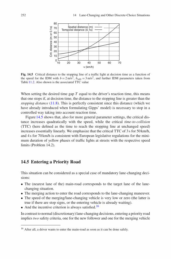
Fig. 14.5 Critical distance to the stopping line of a traffic light at decision time as a function ofthe speed for the IDM with b = 2 m/s2, bsafe = 3 m/s2, and further IDM parameters taken fromTable 11.2. Also shown is the associated TTC value
When setting the desired time gap T equal to the driver’s reaction time, this meansthat one stops if, at decision time, the distance to the stopping line is greater than thestopping distance (11.8). This is perfectly consistent since this distance (which wehave already introduced when formulating Gipps’ model) is necessary to stop in acontrolled way taking into account reaction time.
Figure 14.5 shows that, also for more general parameter settings, the critical dis-tance increases quadratically with the speed, while the critical time-to-collision(TTC) (here defined as the time to reach the stopping line at unchanged speed)increases essentially linearly. We emphasize that the critical TTC of 3 s for 50 km/h,and 4 s for 70 km/h is consistent with European legislative regulations for the mini-mum duration of yellow phases of traffic lights at streets with the respective speedlimits (Problem 14.2).
14.5 Entering a Priority Road
This situation can be considered as a special case of mandatory lane-changing deci-sions:
• The (nearest lane of the) main-road corresponds to the target lane of the lane-changing situation.
• The merging action to enter the road corresponds to the lane-changing maneuver.• The speed of the merging/lane-changing vehicle is very low or zero (the latter is
true if there are stop signs, or the entering vehicle is already waiting).• And the incentive criterion is always satisfied.16
In contrast to normal (discretionary) lane-changing decisions, entering a priority roadimplies two safety criteria, one for the new follower and one for the merging vehicle
16 After all, a driver wants to enter the main-road as soon as it can be done safely.
Fig. 14.6 Illustration of the safety criterion for the decision “stopping/waiting or merging” whenentering a priority road
itself. The latter was not necessary for discretionary lane changes since, there, afulfilled incentive criterion automatically implies safety for the decision maker himor herself (cf. the last paragraph of Sect. 14.3). When formulating the criteria, weassume that the driver of the merging vehicle can anticipate his or her speed vα , thespeeds v f and vl of the follower and leader, and the corresponding gaps s f and sl ,respectively, at merging time (Fig. 14.6)17
merge if s f > ssafe(v f , vα) AND slead > ssafe(vα, vl),
stop or wait otherwise.(14.27)
Problems
14.1. Why the grass is always greener on the other side?Give the reason why, when driving in congested conditions, one generally spendsmore time in the slower lanes and that a lane change does not help. Consider followingsituation:
V2>V1V1
V1L L
The figure shows two-lane traffic with staggered traffic waves of length L con-taining jammed traffic creeping at average speed V1, and the regions in between (oflength L as well) where traffic flows more quickly (V2 > V1) but yet not freely (the
17 Since there are no relevant cars to consider for the alternative “stop or wait”, we have droppedall hats denoting the new situation, for simplicity.
254 14 Lane-Changing and Other Discrete-Choice Situations
congested branch of the fundamental diagram remains relevant). Assume a trian-gular fundamental diagram and negligible speed adaptation times (which is a goodapproximation for the OVM or Newell’s model). Calculate the fraction pslow of thetime one drives inside a wave, i.e., the other lane is faster, as a function of V1, V2,and the model parameters T and leff. Be astounded by the result!
Hint: You can solve this problem by calculating the relative velocity between thedriven speed and the wave velocity. Or simply count the vehicles.
14.2. Stop or cruise?A decision strategy abiding traffic regulation and restricting braking decelerations tominimal values while taking into account reaction times is the following [cf. the IDMcondition (14.26)]: Anticipate if you can pass the traffic light at unchanged speedbefore it turns red. If so, cruise. Otherwise, brake smoothly with constant deceler-ation so as to stop just before the stopping line. When the speed limit is 50 km/h,the minimum duration of the yellow phase prescribed by law is τy = 3 s. What isthe maximum deceleration the legislative authority expects you to use, assuming acomplex reaction time of 1 s?
14.3. Entering a highway with roadworksAssume a highway on-ramp whose merging section, due to roadworks, is nearlynonexistent, i.e., one has to merge at essentially zero speed. The relevant safetycriterion is defined by the OVM with a triangular fundamental diagram (s0 = 0 s,T = 1 s) assuming a safe deceleration threshold bsafe = 0 m/s2. The driver of theconsidered car waits at the merging position while another car approaches on themain-road at 72 km/h. At decision time, the safety condition is just satisfied (the laggap is only marginally greater than ssafe), so the driver begins to merge. Calculatethe minimum deceleration at which the driver of the main-road vehicle has to brakein order to avoid a collision. Assume that the entering car accelerates with 2 m/s2 forthe first few seconds. Furthermore, assume that the driver on the main-road reactsinstantaneously and is able to anticipate the situation perfectly. Discuss whether theOVM safe gap-acceptance criterion is really “safe”, particularly, when assumingfinite reaction times.
14.4. An IDM vehicle entering a priority roadFormulate the IDM safety criterion for merging into a priority road with a stop sign(the initial speed of the merging vehicle is zero). Calculate the safe lead and lag gapsfor the IDM parameters a = b = bsafe = 2 m/s2, T = 1 s, v0 = 50 km/h, and s0 = 0 mif the speed on the main road is 50 km/h.
Further Reading
• Ben-Akiva, M., Lerman, S.: Discrete choice analysis: Theory and application totravel demand. MIT press (1993)
• Gipps, P.G.: A model for the structure of lane-changing decisions. TransportationResearch Part B: Methodological 20 (1986) 403–414
14.5 Entering a Priority Road 255
• Kesting, A., Treiber, M., Helbing, D.: General lane-changing model MOBIL forcar-following models. Transportation Research Record: Journal of the Transporta-tion Research Board 1999 (2007) 86–94
• Nagel, K., Wolf, D., Wagner, P., Simon, P.: Two-lane traffic rules for cellularautomata: A systematic approach. Physical Review E 58 (1998) 1425–1437
• Thiemann, C., Treiber, M., Kesting, A.: Estimating acceleration and lane-changingdynamics from next generation simulation trajectory data. Transportation ResearchRecord: Journal of the Transportation Research Board 2088 (2008) 90–101
• Redelmeier, D., Tibshirani, R.: Why cars in the next lane seem to go faster. Nature401 (1999) 35.