Traffic profiles for audio and data collaborative work systems

University of Wollongong University of Wollongong

Research Online Research Online

University of Wollongong Thesis Collection 1954-2016 University of Wollongong Thesis Collections

1993

Traffic profiles for audio and data collaborative work systems Traffic profiles for audio and data collaborative work systems

W. T. Musangeya University of Wollongong

Follow this and additional works at: https://ro.uow.edu.au/theses

University of Wollongong University of Wollongong

Copyright Warning Copyright Warning

You may print or download ONE copy of this document for the purpose of your own research or study. The University

does not authorise you to copy, communicate or otherwise make available electronically to any other person any

copyright material contained on this site.

You are reminded of the following: This work is copyright. Apart from any use permitted under the Copyright Act

1968, no part of this work may be reproduced by any process, nor may any other exclusive right be exercised,

without the permission of the author. Copyright owners are entitled to take legal action against persons who infringe

their copyright. A reproduction of material that is protected by copyright may be a copyright infringement. A court

may impose penalties and award damages in relation to offences and infringements relating to copyright material.

Higher penalties may apply, and higher damages may be awarded, for offences and infringements involving the

conversion of material into digital or electronic form.

Unless otherwise indicated, the views expressed in this thesis are those of the author and do not necessarily Unless otherwise indicated, the views expressed in this thesis are those of the author and do not necessarily

represent the views of the University of Wollongong. represent the views of the University of Wollongong.

Recommended Citation Recommended Citation Musangeya, W. T., Traffic profiles for audio and data collaborative work systems, Master of Engineering (Hons.) thesis, Department of Telecommunications Engineering, University of Wollongong, 1993. https://ro.uow.edu.au/theses/2558

Research Online is the open access institutional repository for the University of Wollongong. For further information contact the UOW Library: [email protected]

https://ro.uow.edu.au/

https://ro.uow.edu.au/theses

https://ro.uow.edu.au/theses

https://ro.uow.edu.au/thesesuow

https://ro.uow.edu.au/theses?utm_source=ro.uow.edu.au%2Ftheses%2F2558&utm_medium=PDF&utm_campaign=PDFCoverPages

UNIVERSITY OF WOLLONGONG

LIBRARY

Traffic Profiles

For Audio and Data

Collaborative Work Systems

A thesis submitted in partial fulfilment of the

requirements for the award of the degree of

Honours Master of Engineering

(Telecommunications Engineering)

from

U N IVER SITY OF W O LLO N G O N G

by

W .T . Musangeya

BSc(ENG)Hons.(UZ), AM IEE(U K )

elec952, 1993

Abstract

A predictive model of the behavior of multimedia communications systems on

digital broadband networks is needed because, it is through knowledge of the

traffic characteristics of the arrival process, that proper network resource dimen

sioning can be performed to avoid congestion and maintain the network quality

of service. This thesis analyses the traffic from multimedia systems that are ex

pected to become common in the next decade. The traffic is used to develop

models to characterise the statistical properties of such multimedia communica

tions systems.

The analysis was carried out on a real-time computer-supported collaborative

work system, running on ethernet, to which an audio channel had been added.

The audio channel enabled hands-free audio conversations during conferencing

sessions. Data was collected as observations of the transmission time and the

volume of information transferred. The observations were for the networking

interface between the application layer and the operating system.

The model was described in terms of the variability of the packet arrival process

and the degree of correlation between packet arrivals. The squared coefficient of

variation was used to measure the variability of the arrival process. The variables

investigated included interarrival time intervals and the transmission intensity of

the arrival process. The model was presented in two parts: one describing the

l

individual packets’ distribution and the second part looking at traffic bursts.

The model o f the traffic bursts, for both the audio and data arrival process, was

found to approximate a compound poisson process, with the burst interarrival

time distributions indicating negative exponential curves. In the transmitted

audio traffic, the model showed burst distributions consisting of sums of expo

nentially distributed burst interarrival time and transmission intensity curves.

The distributions, for the packet model, were scattered over the time intervals

from 5ms to the threshold value, showing less tendency towards any common dis

tributions. This was observed for both audio and data packet interarrival times

and packet transmission intensity.

The significance of this work is in relation to the modelling of multimedia net

works. It has been shown[Habib 92] that the different types of data sources

transported on multimedia networks can each be modelled as individual Markov

chains. The model presented in this thesis describes the statistical properties of

the variables that would require specification in the Markov chain model. The

distribution curves for the transmission intensity provide for the peak and average

rates, whilst the burstiness parameter describes the time-scale rate of variation.

11

Acknowledgements

I want to express my gratitude to my supervisor, Dr. HWP Beadle, without

whose support and assistance, this study would not have been feasible. I am

grateful for his patience in answering the many questions I had throughout this

study, and explaining most of the concepts I didn’t understand.

I would also like to express my appreciation to the Australian International De

velopment Assistance Bureau (AIDAB) for their financial support, and to the

University of Wollongong, for providing an optimal study environment.

I also thank the wonderful people at the International Council for Overseas Stu

dents who made my stay in Australia an enjoyable experience; and to the many

friends I made, for their moral support.

111

Contents

1 Introduction 1

1.1 Statistical analysis .................................................................................. 2

1.1.1 M otivation..................................................................................... 3

1.2 O b jectives .................................................................................................. 5

1.2.1 CSM A/CD N etworks.................................................................. 6

1.3 About the rep ort....................................................................................... 7

2 Background 9

2.1 Broadband N etw orks............................................................................... 9

2.2 E thernet..................................................................................................... H

2.3 Traffic into a M ultiplexor........................................................................ 12

2.4 Voice sy stem s ............................................................................................ 13

2.5 CSCW s y s te m s .......................................................................................... 13

2.5.1 Multimedia Networks.................................................................. 14

2.5.2 Groupware..................................................................................... 16

IV

2.6 Summary 18

3 System under test 20

3.1 Example sy s te m s ..................................................................................... 20

3.1.1 Shared screen s y s te m s .............................................................. 20

3.1.2 Video drawing m e d ia .................................................................. 21

3.1.3 Talk and W r i t e ........................................................................... 21

3.2 Integrated Voice And Data ................................................................... 22

3.3 Chosen system ........................................................................................ 22

3.4 W S ............................................................................................................... 23

3.4.1 Additions to w s ........................................................................... 24

3.4.2 Starting a new s e s s io n .............................................................. 25

3.4.3 Joining and leaving a session.................................................... 27

3.4.4 Contention P rob lem s................................................................. 27

3.4.5 Session status and information................................................. 27

3.4.6 L im ita tion s .................................................................................. 28

3.5 Mike & sp ea k er ........................................................................................ 29

3.6 S u m m a ry .................................................................................................. 32

4 Numerical Data Collection 33

4.1 Assumptions.............................................................................................. 35

4.1.1 The voice arrival p rocess ............................................................ 35

v

4.1.2 Model Variables............................................................................ 37

4.1.3 Parameter choices........................................................................ 41

4.2 Data Treatment M ethods........................................................................ 46

4.2.1 Chi-square goodness of fit t e s t s .............................................. 47

4.2.2 Log Histogram m eth od .............................................................. 50

4.2.3 Independence (iid) t e s t s ........................................................... 52

4.3 System E nvironm ent............................................................................... 55

4.4 Data c o l le c t io n ........................................................................................ 58

4.4.1 Unix networking ........................................................................ 58

4.5 Data trea tm en t........................................................................................ 00

4.5.1 Choosing interval w i d t h ........................................................... 61

4.5.2 Relative frequencies..................................................................... 62

4.5.3 The upper l im it ........................................................................... 63

4.5.4 Confidence Interval..................................................................... 63

4.6 Data A nalysis............................................................................................ 64

4.6.1 Arrival p a c k e ts ........................................................................... 64

4.6.2 Burst length .................................................................................. 66

4.6.3 Packet s iz e s .................................................................................. 68

4.6.4 Interarrival in te rv a ls ................................................................. 69

4.6.5 Intensity of Transmission........................................................... 76

4.6.6 Response t im e s ........................................................................... $0

vi

4.7 Summary 84

5 Comparison with Packet-Train Model 86

5.1 Traffic m o d e l ............................................................................................ 87

5.2 U tilization.................................................................................................. 90

5.3 Regression A nalysis.................................................................................. 92

5.4 S u m m a ry .................................................................................................. 93

6 Applications 94

6.1 S im u lation s............................................................................................... 94

6.2 Channel C apacity ..................................................................................... 96

6.3 S u m m a ry .................................................................................................. 97

7 Conclusion 98

8 Bibliography 101

A Traffic Profiles 109

B Conferencing systems 119

B . l Audio Conferencing................................................................................... 120

C Broadband Networks 122

C . l Broadband I S D N .......................................................................................123

D Covariance function 125

vii

List of Figures

3.1 WS common w in d o w ............................................................................... 23

3.2 WS conferencing network........................................................................ 28

4.1 Transmission d u r a t io n ........................................................................... 38

4.2 System arrival data m o d e l ..................................................................... 40

4.3 LAN D iagram ............................................................................................ 57

4.4 Data C o llection ........................................................................................ 60

4.5 Upper L im it ............................................................................................... 62

4.6 Received vs Transmitted d a t a .............................................................. 64

4.7 Typical transfer data: combined ws and mike ................................. 65

4.8 Burst Length : arrival data ................................................................. 67

4.9 Packet size Distribution : arrival d a ta ................................................. 69

4.10 Burst Interarrivals : using std. dev. e r ro rb a rs ................................. 70

4.11 Burst Interdepartures : using std dev errorbars .............................. 71

4.12 Packet Interarrivals : using std dev errorbars.................................... 72

4.13 Packet Interdepartures : using std dev errorbars.............................. 73

vin

4.14 Burst Intensity : for combined ws Sz audio(std. d e v ) ....................... 77

4.15 Burst Intensity : arrival process using std. dev................................... 79

4.16 Packet Intensity : arrival process using std. dev................................. 80

4.17 User response and idle time : combined system with std. dev. . . 81

4.18 Idle time : std dev errorbars.................................................................. 82

4.19 User Response time : std dev errorbars.............................................. 83

5.1 Network U tilization.................................................................................. 91

A .l Typical arrival data: ws and s p e a k e r ..................................................... 109

A .2 Typical departure data: ws and speaker..................................................110

A .3 Burst Length : for departure d a ta ........................................................... 110

A .4 Packet size Distribution : departure d a t a .............................................. I l l

A .5 Packet size Distribution : combined ws and audio d a t a .................... I l l

A .6 Burst Interarrivals : ymin/ymax e rro rb a rs ........................................... 112

A .7 Burst Inter departures: ymin/ymax errorbars........................................112

A .8 InterBurst time intervals: combined ws and a u d io .............................. 113

A. 9 Packet Inter arrivals : using ymin/ymax e rro rb a rs .............................. 113

A. 10 Packet interdepartures : using ymax/ymin errorbars...........................114

A. 11 Interpacket time intervals: combined ws and au dio .............................. 114

A. 12 Burst intensity: combined w s /au d io (ym in /ym ax ).............................. 115

A. 13 Burst Intensity : arrival process using y m in /y m a x .............................. 115

A .14 Burst Intensity : departures using std. dev............................................. 116

IX

A. 15 Packet Intensity : arrival process using y m a x /y m in ....................... 116

A .16 Packet Intensity : departures using std. dev........................................117

A. 17 Packet intensity: for combined ws and a u d io .................................... 117

A. 18 User response and idle time : combined system ymin/ymax errors 118

x

List of Tables

4.1 Chi-square goodness of fit r e s u lt s ........................................................ 51

4.2 Contingency Table : iid tests .................................................................. 52

4.3 Chi-square iid test results ..................................................................... 55

4.4 Squared coefficient of variation.............................................................. 75

4.5 The Equations for curve f i t ..................................................................... 85

5.1 The Network Traffic M od el...................................................................... 89

xi

Chapter 1

Introduction

The design of computer networks involves the design of the transmission circuits

between the hosts as well as the design of the switching connecting any two or

more transmission lines within the network. Switching routes data arriving on an

incoming circuit to the appropriate outgoing line for forwarding to it’s destination.

The design of transmission circuits can be for point-to-point communication or

broadcast communication channels. In the former, a circuit is used to connect

two switches so that only indirect communication can be used between hosts who

are not directly connected by a circuit. Broadcast, on the other hand, requires

a single circuit that is common to all the hosts. In this case the transmitted

messages are received by all connected computers and each host only copies the

messages if the messages are directed to that host’s address.

Other issues involved in computer network design are

1

• error detection and error correcting mechanism

• preservation of the order that the messages are sent.

• method for establishing connection with the desired host and terminating

the call when done.

• method of data transfer i.e. unidirectional or full duplex operation.

• control of the rate of receiving or sending messages i.e. flow control.

• limits on the length of messages that can be handled i.e. assembling and

disassembling of messages.

• routing decisions where more than one route exists between the hosts re

quiring data transfer.

• channel and bandwidth allocation.

• contention problems in shared channel systems.

1.1 Statistical analysis

In all these design issues, the characterisation of the carried computer signals

takes an important part. For example, to properly allocate bandwidth, it is

necessary to know the probability of a frame being generated in an interval, say,

St. This probability is calculated as A St where A is the arrival rate of new frames.

2

It is therefore essential to understand the statistical properties of the signals so

that predictions can be made on the variation of the data.

The predictions possible with the statistical information make it easy to allocate

network resources in anticipation of demand. This is very desirable especially

with the imminent broadband intergrated services digital networks (ISDN) and

the asynchronous transfer mode (ATM) switching technology which are designed

to offer bandwidth on demand. A brief description of broadband ISDN is given

in section C .l.

1.1.1 Motivation

The statistical analysis carried out in this project is an attempt to change the

sample numerical traffic data into meaningful facts that can aid in network design

decision making. From this analysis, generalizations can be made with regard to

the traffic profiles of similar computer applications.

The use of graphs and tables to present the collected data and the deduced traffic

profiles, gives a clearer, easy to understand picture of the traffic characteristics.

The basic statistical element in the investigation will consist of ratio data in the

form of transmission time and the volume of the information transferred. From

this data, the time interval data is derived.

The ratio data is obtained from several executions of shared workspace applica

tions. A shared workspace is defined[Guan 88] as a collection of objects belonging

3

to some work group and the software tools that are required for their manipu

lation. Limitations of time and the large varieties of available shared workspace

programs, make it impossible to investigate the complete population. Thus, only

a sample is used, consisting of observations of one particular shared workspace

application. Shared workspace applications are synonymous with Computer Sup

ported Collaborative Work(CSCW) systems. CSCW systems allow joint use of

computer based material, providing multi-point computer conferencing. They

achieve this by presenting a common view of the work surface to which simul

taneous access is given to the connected participants. Several CSCW products

have been developed; a few of them are described in section 3.1. Section 2.5.2

discusses CSCW in more detail.

CSCW sessions can be considered “Multimedia” since they involve, in addition

to the CSCW applications, audio conferences and sometimes video conferences.

Given these different types of data, all carried on one multimedia network, quality

of service(QOS) becomes vital in preserving the communication content. It has

been shown[Sriram 86] that packetized voice communication is sensitive to jitter

and that it’s quality decreases with an increase in the system response times.

This is especially true when the network is congested. Data communication,

on the other hand, requires stringent error characteristics. These are conflicting

requirements and hence the need for investigation into the statistical nature of

the traffic generated in systems where audio and data are combined.

4

So far research on shared workspaces has concentrated on implementation, re

sulting in a wide range of cscw products being developed. With all these product

developments, it is time that attention focussed on the statistical nature of the

network traffic generated by these new applications. This research is necessary in

order to design networks that are well qualified to carry multimedia and CSCW

traffic. The resulting traffic models would then aid networked multimedia sys

tem design to better dimension the network. This would provide information on

how well these systems work on the existing networks or information on which

proposed new networks are better suited to these systems.

1.2 Objectives

The objective of this research is to collect and analyse the statistics of a col

laborative work system where several users receive audio and visual information

simultaneously. The objectives are to design the system, measure the performance

and characterize the performance to achieve an overall goal of understanding the

traffic characteristics of the service. The network statistics of the traffic that

ensue are then analysed to develop a workable traffic model.

The conferencing system is developed on the Unix operating system using the X

Window to run on the Sun SparcStation. The audio channel in this system is

provided through the audio input and output facilities offered by the Sun Spare-

Stations. It is designed to allow communication between two or more users. This

5

system offers flexibility and the ease of use that comes with voice conversations,

e.g. psychological cues in the tone of voice, length of pauses, etc, in addition to

the ability to share visual material through the computer terminal. CSCW data

is carried on Internet’s connection oriented Transmission Control Protocol (TC P)

stack, whilst the audio uses the connectionless User Datagram Protocol (UDP)

stack. The collaborative work system does not use the broadcast and multicast

protocols, relying only on polling and sequential delivery of data.

The research uses ethernet because of it ’s availability on a larger scale. It is one of

the most widely used networks and it presents the worst case in network perfor

mance due to the influence of the network’s backoff algorithms which introduce

undesirable delay jitter on voice packets. Ethernet does not offer any priotization

of voice packets over data packets.

1.2.1 C S M A /C D Networks

Ethernet is a carrier sense multiaccess bus network (C S M A /C D ) with collision

detection. It works by having the source hosts detecting the carrier on the bus.

Absence of carrier signal on the bus is interpreted as a go - ahead for transmission.

W hen the host senses the absence of carrier it acquires the bus by transmitting

it ’s information. All other hosts then wait until the transmission is completed.

If two or more hosts transmit simultaneously i.e. a collision occurs, both stop

transmission and wait a random time before attempting retransmission. Colli

6

sions are detected when the sending hosts read back their information from the

bus to check for correct transmission. In case of collisions, instead of receiving

it ’s own information a host receives a mix of i f ’s information and the other host’s

information. The detecting host then jams the bus so that all intending source

hosts have to backoff for a random time that may be determined by some function

e.g. the binary exponential backoff algorithms. A typical slot time of 38us round

trip bit propagation time[Stallings 89] is the time it takes for the first bit of the

second host’s transmission to travel to the first host.

1.3 About the report ...

The report begins with brief background information on past research into traffic

characterisation in Chapter 2. This chapter also introduces the topics of group

ware and multimedia networks.

Chapter 3 presents an overview of the CSCW systems that have been developed

so far, and presents a detailed description of the developed cscw system’s technical

architecture.

Chapter 4 gives the procedures used to gather the traffic statistics, the environ

ment in which the experiments were carried out and the analysis of the results

that were obtained.

Next is discussed the modelling methods employed, leading to a summary and

7

the presentation of the developed traffic model in Chapter 5.

Chapter 6 gives examples of situations to which the model can be applied.

Chapter 7 concludes the research followed by the bibliography list and a set of

graphs in the appendix.

8

Chapter 2

Background

The statistical analysis of computer-generated traffic has been carried out over

the years by several researchers. Though none of the work investigated the traffic

generated from shared workspaces, most of the research has been on the perfor

mance of available networks (ethernet, token ring[Yang 92], etc) in transporting a

combination of different traffic types like audio and data traffic [Nutt 82] or voice

and video traffic[Habib 92]. There has also been some research on modelling data

as groups of packets [Jain 86].

2.1 Broadband Networks

Traffic profiles for voice and video traffic sources have been investigated [Habib 92]

for use on broadband networks. In their investigations, Habib and Saadawi ex

pressed how the variability of the variance lead to queueing delays, contributing

9

to congestion. The aim was to find analytic models to characterise correlation

and burstiness o f multimedia traffic. They described the voice process as a bursty

Markov process, quoting the squared coefficient of variation(SCOV) figure of 18.1

from [Sriram 86]. Bursty traffic was defined as one that exhibits a high degree o f

variability compared to that o f the poisson process. The packet arrivals during a

talk spurt were modelled as a Bernoulli distribution and the duration of each talk

or silence state modelled as a geometric distribution. For multiple voice sources, a

markov chain of M states was used with the state as the number of voice sources

in the talk state. To represent sources with different traffic characteristics (

multimedia traffic), independant and identically distributed Markov chains for

each source were suggested. The SCOV, as defined in [Sriram 86], was applied to

the continuous time model of the arrival process and the index of dispersion for

counts (IDC) used for dici;ete-time model. The IDC is defined as \

with N t as the number of arrivals in an interval length. It is the variance of the

number of arrivals in an interval t normalized by the average number of arrivals

in that interval length.

10

2.2 Ethernet

Nutt and Bayer [Nutt 82] covered the performance of ethernet on a combined

voice and data load. A simulation model of the ethernet network was used.

Their experimentation was concerned with adapting ethernet to carrying com

bined voice and data effectively and efficiently. They tested their model using

overload conditions specified by Metcalfe and Boggs [Metcalfe 76] and the packet

size and interarrival time observed by Shoch and Hupp[Shoch 80].

They formulated two types of networks; one that distinguished between voice

and data traffic and the other which didn’t, and adopted different backoff algo

rithms for each type of network. Acknowledging that data can tolerate delays

during congestion periods, and that voice packets have real time limits, a ran

dom algorithm was applied to voice and a binary exponential algorithm to data

packets. The random algorithm dynamically determined the backoff time using a

uniform distribution function which was sampled by some predetermined value.

The binary exponential backoff algorithm has backoff times growing exponentially

and allows for congestion conditions, achieving recovery of the network through

degradation of the network performance. Another suggestion given was the use of

the binary exponential algorithm for both voice and data packets but with twice

the value of the exponential distribution mean for data packets. The experiments

covered in the paper suggested that both the above algorithms failed under heavy

traffic conditions during voice applications, resulting in delays greater than their

11

3 0009 03100 9546

threshold defined as 5ms. Their tests involved simulated loads instead of actual

data, with approximated interarrival time and packet size distributions.

2.3 Traffic into a Multiplexor

There has also been research covering the analysis of the performance of packe-

tized voice and data traffic on a statistical multiplexor[Heffes 86]. The number

of arriving voice packets is modelled as a geometrical distribution with exponen

tially distributed talk and silence states, in an interval of length 16ms. From this

model and using the Laplace-Stieltjes transform (LST) [Heffes 86], it is shown

that the SCOV of the interarrival time is given by

SCO V =

for both a single voice source and a superposition of an arbitrary n voice sources.

The combined arrival process of packetized voice and data streams is modelled

as a Markov Modulated Poisson process. This is a stochastic process where the

arrival rate Aj of the process is equal to the state of a continuous time two-

state Markov chain, i.e. the arrival rate of the process is equal to the Poisson

arrival rate of the current state j . The parameters specified in the model are

the mean arrival rate (noting that A-1 is the mean time between arrivals), the

variance to mean ratio of the arrivals in an interval, the same ratio long-term,

and the skewness parameter given by the third moment of the number of arrivals

12

in an interval. Simulations of the model provided results similar to those of a

deterministic process, as described in [Sriram 86]. This was using fixed voice

packet lengths of 64 bytes, geometrically distributed data packet lengths with

mean 50 bytes, and data packets arriving as a Poisson process. The paper also

observes that the correlation structure of the superposition structure is defined

well by the variance - time graph.

2.4 Voice systems

Models to describe the statistical properties of packet voice systems were inves

tigated by Daigle and Langford [Daigle 86]. Their paper models the voice packet

generation process as a Poisson process with the number of active voice sources

represented as a continuous-time Markov chain. It also investigates fixed packet

generation rate with first, a semi-Markov process and then, with a uniform ar

rival model. The analysis was strongly oriented towards developing a queueing

system model rather than modelling the packet generation and subsequent arrival

process parameters.

2.5 CSCW systems

CSCW systems are arguably a new application that is rapidly expanding in re

cent years. More and more CSCW systems are being integrated with audio and

13

video information for transmission on a single multi-media network. It is there

fore worthwhile to look at the behaviour of multimedia networks to enhance our

understanding of the traffic profiles from CSCW systems. Multimedia networks

provide an integrated communication media for data sources. They range from

the integrated transportation of audio and data on a data network to the trans

portation of traffic from disparate data sources on a single network. The following

literature gives a brief discussion on traffic characteristics of multimedia networks,

and introduces CSCW systems as a branch of multimedia networks. This liter

ature should give an incite into what to expect for the traffic analysis in this

research.

2.5.1 Multimedia Networks

The diversity of the data sources on multimedia networks may include variations

in the speed of data, deviations in the length of the data and variations in the rate

of arrival of the data packets [Schwartz 77]. This is a different scenario from bulk

data transfer where transfer occurs at an average bit rate and normally consists

of data of the same type. The main information sources in this scenario are voice,

video, graphics, and high quality audio. The goal is to achieve integration and

synchronization without performance degradation. This sets limits on the types

of data sources that can be transported as well as on the number of data sources

that can be combined at any one time. Traffic profiles have to be described in

14

order to model such points of integration.

Simple examples of systems that would require integrated communication media

and hence are multimedia are adding video to electronic mail or moving video

conferencing into a window on a computer screen.

Multimedia information flows can be grouped into three types.

• User to document information flows as in e-mail

• User to computer as in information systems, accessing databases through

graphical user interfaces.

• User to user information flow as in CSCW systems accessed through con

ferencing or training sessions.

Multimedia network characteristics

As multimedia systems carry voice and video, which are essentially continuous

communication media, they therefore require continous data transfers over long ^

periods of time.

In order to keep each presentation device’s fixed data ratio, multimedia networks

may require event-driven or on-going synchronization relationships between the

real time data channels. An example of where this would be necessary is the

transportation of a moving picture signal, where the separately stored audio signal

is correlated with the video signal and the trasmission requires synchronization

15

to maintain intelligibility.

Because of the wide variety of traffic types transported in multimedia networks, a

particular QOS is required. A dynamic supply of network resources like network

bandwidth, processor time or disc bandwidth should be guaranteed. Provision

should be made for control of this QOS so that it is possible, for instance, to

sacrifice the QOS or to reject a request for service in the face of insufficient

resources. These are called call admission requirements.

2.5.2 Groupware

Computer-based group activities are found in the area of multimedia applications

that consist of user to user information flows. These are presented as real time

computer conferencing systems with a variety of tools added in; tools like inte

grated voice and data communication, joint-editing facilities and collaboration

tools. Further information on computer conferencing system is given in appendix

B. The objective is to provide interaction similar to that which occurs in face

to face drawing processes. These computer based group activities are referred

to as groupware, CSCW systems or shared workspaces. They provide integrated

support across group activities regardless of the users’ geographical locations, co

ordinating the dynamic sharing of screen tools in a real time nature. The data

sources that groupware may combine are computer data, text, and remote image

service feeds. It is this ability to support collaborative projects across the users’

16

networks that may make it the pillar of activities in Publishing Houses, Military

Agencies and R Sz D Laboratories [McQuillan 92].

Group interaction requires continuous media transmission for applications requir

ing simultaneous display of information on several displays. This is called group

communication. In other cases, a single operation applied to a number of displays

may be required and this is an example of group invocation.

The main applications of groupware are in conferencing [McQuillan 92] and train

ing. Groupware requires real time two way transmission with high bandwidth

and a guaranteed QOS - i.e. low delay with low variance and low data loss. The

successful acceptance of groupware is based on it’s ability to combine existing

individual work practices with the collaborative work mode.

In designing groupware, it is necessary to identify the members of a work group

that have a joint need to communicate. A deep understanding of the human

characteristics is required, as is the organisational aspects like the structure of

an organisation. The involvement of the user in the design process is important.

Group dynamic aspects like decision making or the collaboration process must

be considered [Johansen 88]. Collaboration can be by group invocation or group

communication.

Video conferencing and electronic mail are examples of the communication mech

anisms that support group work. Like groupware, they offer shared workspace

17

facilities, shared information facilities as in multi-user databases, and facilities

that augment specific group work processes like co-authoring of documents or

idea generation [Hopper 91].

Groupware, like everything else, has to undergo usability testing for wider accep

tance. It demands connectivity and availability at all times. These are the factors

that increase the efficiency of searching and exchanging information. An example

is given [Brand 88] of a user who multicasted an e-mail asking for information

on a topic and received several responses from all over the world the next day.

Example uses of such systems would be in the circulation of memos and reports,

and for group revision or group review of some subject matter.

On-line editing is another widely accepted form of groupware. It finds applications

in message systems, procedure processing systems, screen sharing systems and

calendar systems.

2.6 Summary

Looking at the research that has been carried out in traffic characterisation, it is

clear that most models of packetized voice signals have been presented as Markov

chains. This has been due to the ease with which the Markov Chains are applied

to queueing network analysis. The missing information required now is how the

Markov chain is defined for particular applications. This may be in the form of

18

statistical properties for interarrival times, data rates and how bursty the arrival

process is.

The application whose traffic characteristics are to be investigated has been in

troduced as a CSCW system with added voice communication. The next chapter

discusses this system in detail and gives a brief description of other CSCW sys

tems that have been developed.

19

Chapter 3

System under test

There have been several CSCW systems developed. The following sections de

scribe some of the developed systems and gives the criteria used in choosing a

CSCW system for traffic analysis.

3.1 Example systems

As mentioned in section 2.5.2, CSCW systems present a common view of the

work surface allowing simultaneous access by the participating users. Several

different shared views can be used. Below are a few examples.

3.1.1 Shared screen systems

Timbuktu remote is an example of a shared screen system [Farallon 91] which

is also similar to the shared window system[Lauwers 90]. Multiuser editors like

20

GroupSketch[Greenberg 92] and shared text editors[Neuwirth 90] also use a shared

screen as a common view.

3.1.2 Video drawing media

An example of a shared video drawing media is the TWS (TeamWorkstation),

developed by Ishii and Miyake [Ishii 90], [Ishii 91]. The TWS integrates the

computers and the desktop workspaces. It also provides distributed users with

an open shared workspace. TWS is designed in such a way that the individual

workspace images are overlaid. Each individual continues to use their application

programs. At the time of writing their paper, TWS had not been tested with a

larger variety of tasks. According to [Ishii 91], TWS is not aimed at replacing

groupware. It supports a broader range of dynamic collaboration activities which

are not supported by existing groupware. Their recent work[Ishii 93], ClearBoard,

is a shared drawing medium that supports gaze awareness in remote collaboration.

3.1.3 Talk and Write

Talk is a visual communication program which copies text lines from one terminal

to another user. It is run on Unix computers. Once connection is established,

two users may type simultaneously with displays on separate windows.

talk uses a server talkd to listen at the udp port and a tcp connection is made for

the conversation.

21

Write is a program similar to talk except that it uses the same screen for both

users and does not cater for simultaneously sent messages. The users have to

develop a system of letting the other know they are waiting for a response e.g.

the use of over or over and out.

3.2 Integrated Voice And Data

Integration of voice and data is usually achieved through voice digitization. For

better transmission quality and efficiency, the voice digitization at the source is

then followed by the use of a digital transportation to the customers’ premises.

An example product designed to handle both voice and data traffic is Netrunner[Salamone 92 J

developed by Micom. It is a system that uses data and speech compression to

boost throughput. It also handles voice and facsimile traffic in addition to linking

Local Area Networks.

Voiceview[Radish 92], is an application developed by Radish Communication Sys

tem Inc. which can transmit data during a voice call on analog lines. One has to

make a voice call and then downloads data by the pressing of a button.

3.3 Chosen system

In choosing a collaborative work system for traffic analysis, it was desired that

it be representative of most other CSCW systems as well as being versatile and

22

simple to use. Thus the following system(section 3.4) was chosen because it con

tains the basic building blocks of many other advanced system, and also because

of it ’s suitability for an educational environment.

Figure 3.1: WS common window

3.4 W S

The developed collaborative work system, which will now be referred to as ws,

is a real-time computer conferencing system, adapted from the window scrawl

program wscrawl written by Brian Wilson[Wilson 92] of Hewlett-Packard. Ws

was developed and tested within a university local area network environment

on the SUN SparcStations. Figure 3.1 shows a workstation screen during a ws

session. The ws window is the large one containing the hand drawn HELLO. The

content of the ws window is shared with all the users in a session. All the other

23

windows on the screen are private. The system is designed for use on the Unix

operating systems connected to the internet domain. Figure 3.2 shows how ws

uses the network, ws uses the sockets and the TC P/IP protocol stack to provide

a reliable two way virtual circuit connection between several conference members.

The required windows were created using the X Window system. The time to live

address field was left set to the default of 60 seconds to allow all data to be sent

regardless of delays of up to 1 minute. If a packet is delayed beyond this value it is

discarded. This is desirable in order to stop transmission of such delayed packets

whose reconstruction at the destination result in unintelligible conversation.

Ws is an X-Window based application that creates a collaborative computing

environment by allowing controlled shared access to a few chosen objects. The

program provides a common white board (see figure 3.1) in the form of a com

puter window, allowing participants to display images, scribble and use gestural

expressions in referring to material displayed on the window. It thus provides

facilities that would be required in any face-to-face meeting.

3.4.1 Additions to ws

Realizing the limitations of ws for collaborative work and tutorial presentation,

the following features were added,

• the snapshot function; Snapshot allows the user to grab any window image

on the screen and paste the image onto the common viewing area. It is

24

implemented on the same principles as the window dump utility, xwd, but

uses routines like read-image-on-disk which are already available on ws to

process the images.

• the slide show function; slide show provides the means to store several

images as files in a directory. The slides can then be displayed consecutively

on the common viewing area for use in presentations. It is implemented on

similar base to snapshot. It produces a menu that allows the user to make

choices on the activities that can be done, activities like store slide, show

slidej next slide, etc. When the slide show is running, only the user who

initiated it has control. The rest of the participants can view the slide and

use the audio channel for discussion. To allow the rest of the users to use

gestural expressions on the displayed slide, the user quits the slide show.

This leaves the current slide displayed and enables all the users to use the

ws tools whilst reviewing the displayed slide.

• The size of the window was reduced to allow full display on the smaller

Macintosh screen.

3.4.2 Starting a new session

The parameters required to start a collaborative work session are a list of the

participants to be included in the collaboration and optional values to override the

default settings of the creation of windows. These are specified at the command

25

line on running the program. Here a session is defined as the participants engaged

in the collaboration. Additional participants can only be added to an existing

session by those already in session and this can be done at any point in the

collaboration and by any connected participant.

For every display that is to be involved in the session, the ws program opens

three windows on the screen; one for window control, one for displaying status

information and a shared white board for displaying user activity. After initial

izing the windows, ws uses the select system call to monitor the input of all the

displays’ session windows for either, the occurrence of an event or timeout.

The events, monitored by the select function, can be input from the keyboard,

the mouse, the control window (-for resizing), the server, the socket, etc. When

an event occurs, ws scans the users’ displays for the event, and then performs the

appropriate action. If the event involved typing, pointing or dumping of an image

on the screen, ws replicates this action on every window opened by the program.

Functions for opening text files, reading or saving bitmaps and images are pro

vided. One can also choose the pen colour or width and select style and font

of the typed characters. A rubber pointer allows gestural expression through a

unique label (i.e. the display name) that is visible on all displays, at the point of

reference, making explanations clearer. In addition, ws provides basic functions

for sketching, typing, erasing, drawing shapes and clearing windows.

26

3.4.3 Joining and leaving a session

Ws is executed at only one of the workstations involved in the collaboration and

provides facilities for adding new participants to an already established session.

One can also withdraw from the session without affecting the continuity of the

CSCW session.

3.4.4 Contention Problems

Unlike some other systems[Guan 8 8 ], no token is provided to control the users’

inputs to the common window. The only restraint available is the display of a

please wait message displayed on all windows when the computer is busy. This

occurs, for instance, when processing a request or updating the participants win

dows at times when large data transfers are necessary and are taking a long time.

All participants have equal status during a session and hence can leave the session

at any time without the need to elect a new /e«der[Guan 8 8 ].

The problem of more than one participant accessing the same tool at the same

time is avoided by the fact that ws uses polling (and the select function) to process

any event occurrence.

3.4.5 Session status and information

Information about the number of current displays open and their identities are

displayed on the status window. This information is updated every time a user

27

joins or leaves a particular session.

Figure 3.2: WS conferencing network

3.4.6 Limitations

Figure 3.2 shows the implementation of ws with the process and data centralized

at the session creator’s machine. Inputs typed by any user are forwarded to

the session creator program and the output, generated from the session creator

machine, is sent to all displays in the session. This requires larger bandwidths and

poses security risks as users are allowed access to the session creator’s directory.

Another limitation is in the design of ws, where the users cannot use system calls

or system objects except those that have been incorporated into the application

itself, thus only tools like file input/output or the slide show which are designed

within ws, can be used.

Keeping the window display consistent is another source of problems. As already

28

mentioned, ws displays a please wait ftag on all displays whilst updating the users’

displays. This results in larger delays or session response times. This problem

brings out the superiority of replicated implementation over the centralized im

plementation. With replicated implementation[Guan 8 8 ], only the input from a

user is sent to the session creator’s machine. This machine then sends a message

to all participants, so that each station regenerates the same input and has it’s

local program producing the output data locally. This, in addition to shorter

response times, would require less bandwidth between the users’ machines.

3.5 Mike 8¿ speaker

The audio component of the collaborative work system is provided by two pro

grams, mike and speaker [Walker 91]. Mike and speaker are designed to work on

the Sun SparcStations providing voice communication using the terminals’ audio

facilities to packetize the voice signal.

Mike does the recording and transmisión of the voice signal. It supports both

real time audio and pre-recorded sound samples, and uses the recordQ function.

This function reads audio from the device file /dev/audio so that mike holds this

device when it transmits data. Normally sound is transmitted at the standard

rate of 8000, 8 -bit samples per second, to give the 64kb/s rate.

Voice coding techniques, like silent interval detection or TASI (time assigned

29

speech interpolation) can be used for bandwidth reduction to values as low as

16kb/s.

Mike, however, can be configured to transmit compressed audio at 4000, 8 -bit

samples per second reducing bandwidth to « 32kb/s, a value suitable for trans

mission on 56kbit/sec links. This compression is achieved by transmitting only

the even numbered sample points i.e. halving the number of samples. Speaker

then does a linear interpolation between the received compressed audio points

to reconstruct the full signal. The resulting lower quality audio is more intel

ligible than the effect of lost words and erratic pauses that would occur if the

uncompressed signal was transmitted on lower bandwidth lines.

Speaker is the receive and playback component of the communication system

responsible for the reconstruction of the sound samples. A workstation will not

be able to receive audio communication if speaker is not running on that terminal.

Speaker creates a socket, binds the socket to a port and then listens for connections

to the socket to be made by the mike program. It then uses the soundtool facilities

on the Sun Sparcstation, which write to the device file /dev/audio on receiving

sound samples. It releases the device after a 20 second timeout if no samples are

received. A gain control tool, x.gaintoolQ can be run in conjunction with speaker

to permit interactive setting of the audio playback level. It can also be used to

switch the received audio from the computer speaker to the headphone jack.

By setting the recording and squelch levels to allow the sending of data only

30

when someone is speaking, it is possible to emulate a collection of speakerphones

sharing a single connection in a conference. The results are intelligible only if

one person speaks at a time; because speaker interleaves the audio received from

multiple sources packet by packet. A mixer program would be required to remedy

this.

Hangover detection and silence suppression were used wehen the mike and speaker

data was collected. The mike program averages the signal on a collected voice

sample, and compares the average against a threshold. When the sample average

is below threshold, it is compared with the previous samples to determine if it

represents the end of a talk period. In the case that the sample represents the

end of a speech burst, the sample is transmitted. If a second sample is received

next and found to have energy lower than the threshold, this second sample is

taken as noise occurring during a silence period and is discarded. Hangover was

implemented to prevent clipping of the voice signal at the end of sentences.

Both Mike and speaker use the datagram sockets in the internet UDP/IP domain,

which does not give any flow control or acknowledgments. As voice communica

tion is real time, retransmitting a lost packet (if at all possible) will only degrade

the quality of the reconstructed sound. Lack of acknowledgments, on the other

hand, are a disadvantage in that no warnings are given in the case of breakdown

in the communication line, or the fact that speaker might not be running on the

remote displays. No flow control is possible should the need arise to control the

31

rate at which packets are dispatched during the session. The program releases

the audio device if it does not receive packets within a minute. This allows some

other applications to use the audio tool during the periods of inactivity. Speaker

uses the usleep function to wait for the received packets to play before grabbing

the next set of packets.

3.6 Summary

Detailed descriptions of the CSCW and audio systems designed have been given.

Looking at the structures of the CSCW systems described, it is clear that ws

provides the basic building blocks covering most aspects of CSCW systems, the

exception being the video drawing systems. In the next chapter, the experi

ments carried out to collect the traffic data generated by the ws and the audio

communication programs are reported.

32

Chapter 4

Numerical Data Collection

The measurement of performance of voice and data integration systems is centred

on the preservation of good quality voice conversation. In this research quality

was assessed subjectively by determining the degree of discomfort that the par

ticipants felt as regards clarity of reconstructed speech, the system delay, and

how easily they felt comfortable with the application system.

One measurement variable is the burstiness of the arrival process which gives an

indication of how variable the arrival process is. It is characterized by the burst

length and the burst distribution in time. From this variable, the probability and

intensity of an arrival can be derived.

The interarrival times between consecutive arrivals are critical in the reconstruc

tion of the transmitted sound. This is because if arrivals suffer uneven, long

delays they may result in lost packets which transform to speech gaps on recon

33

struction, rendering the conversation unintelligible. The mean and variance of

the interarrival time intervals are used to characterise the performance of the

network.

The delay experienced by a packet through the network can also be used to

determine the appropriate value to be used in the time to live field in the internet

datagrams, for example, so that the transmission of excessively delayed packets is

stopped. Delays can be due to packet generation time, the queueing delay before

departure, transmission time through the network and the reception time at the

intended destination. The presence of gateways that introduce uneven delays in

networks as well as network characteristics, like random backoffs after collisions

in CSM A/CD networks, all add to the absolute delay value. Thus the chances of

non-uniform delay or jitter being experienced from packet to packet are of high

probability. The mean and variance of this type of delay are required to be low,

to prevent disruption of voice communication. Data packets, in contrast to voice,

are more sensitive to error control and recovery techniques than to delay. Because

of these differences, it is desirable to give priority of transmission to the digital

data resulting from voice digitization in relation to the rest of the digital data.

This would mean that hosts transmitting voice information get more chances of

transmitting than the rest of the machines. Methods to achieve this on Ethernet,

are discussed in [Nutt 82] .

The probability of losing a voice packet due to network delay is measured by

34

setting a threshold delay value above which, the resulting reconstructed sound

is of an unacceptable quality. In [Malek 88 ], the value of this threshold delay,

with reference to an absolute delay, was given as 150ms for a local area network.

The higher the probability of losing a packet, the less desirable it is to use the

voice application programs. The probability is more a function of the network

conditions than of the application programs.

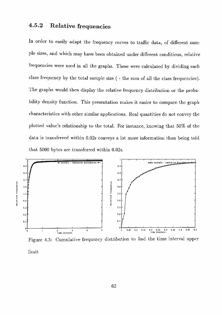
This chapter presents the traffic profiles and gives an analysis of the results ob

tained from the execution of the collaborative work application programs de

scribed in the previous chapter.

4.1 Assumptions

The following briefly introduces the traffic model assumed for the collaborative

work application and describes the variables that arise from the model.

4.1.1 The voice arrival process

As discussed in the previous section, the traffic characteristics of voice packets

differ from those of data packets. Voice communication involves real time trans

portation of data traffic and consists of periods of talking and periods of silence.

In most systems, packets are generated in the talking state only.

For the voice inter arrival time intervals, our analysis assumes exponential distri-

35

bution with mean values A and ¡i for the arrival process during the talk and silent

states respectively. This means that the arrival process is a poisson process, i.e.

has unpredictable talk states. Similar assumptions were done in [Yang 92] and

[Habib 92]. It would be difficult to determine these mean values directly because

the orders of magnitude of the time values involved are very small. Also, since no

packets are generated in the silence state, it makes the measurement parameters

even smaller. By adopting the derivation of the model in [Yang 92] which as

sumes a Poisson batch arrival process (or compound Poisson process), equations

for the mean and variance can be derived. The batches are defined as groups

of packets which may have randomly varying sizes. The inter arrival times were

assumed to be independent and identically distributed. It is also assumed that

the distribution of the burst lengths or the batch sizes remains constant. This

means that the traffic will increase as the number of users in a session increases,

but the characteristics of the traffic generated by each user or monitored at any

one port, will remain constant[Forys 90].

If z is a random variable representing the interarrival time, Q. Yang et. al.

[Yang 92] showed that the mean of the interarrival distribution, E[x\ is given by

' I R i <4 1 >

and it ’s second moment given by the following equation

- 2m ) (4-2)

36

where E[Nb] is the mean batch size and A& the mean batch interarrival time of a

batch arrival process. iV& is the number of packets generated during a talk state.

4.1.2 Model Variables

Figure 4.2 represents the assumed model for the arrival process of the WS data

stream. In the analysis, a packet refers to the number of bytes that were trans

ferred for the application program by the operating system, during any one oper

ating system call request. The data stream model therefore looks at the interface

between the application layer and the operating system. The mapping of this

interface to the actual network is discussed in section 4.4.

The definition of a burst used in the model, was as a group of packets in which the

period of inactivity between any two consecutive packets is smaller than half the

width of one such packet [Jackson 70]. Looking at the packet length distribution

of the application programs investigated, the average packet length for all the

transferred data was found to be 715 bytes with the nearest observed packet length

being 1048 bytes with average effective transmission time of 0.084172 seconds.

The definition of a burst was based on the average effective time it took to

transmit this 1048 byte packet. Thus the threshold value was taken as 42.086ms

(half the transmission time) in the following analysis. The burst was then defined

as a group of packets in which the period of inactivity between any two adjacent

packets is smaller than 0.042086 seconds.

37

A p p lic a t io np r o g r a m

A p p lic a t io np r o g r a m

r e a d /w r it o s y s t e m c a ll

e f f e c t iv e t r a n s m is s io n t im e

s t r a c e c o n t r o l p r o g r a m r e c o r d s s ta rt time-Sc. f o r w a r d s c a l l to o p e r a t in g s y s t e m

re tu rn in g c o n tro l

s t r a c e c o n tr o l p r o g r a m r e c o r d s f in is h tim e , b y t e s tr a n s f e r r e d & fo r w a rd s c a l l b a c k to a p p lic a t io n p r o g r a m

U n ix O p e r a t in g S y s t e m t r a n s f e r s th e d a t a In b e t w e e n o t h e r t a s k s

Figure 4.1: Transmission duration : indicating the effective transmission time

Also, for our purposes the transmission time referred to the effective time it took

the control program, strace, to detect the onset of a request for a system call

to the time the operating system returned control to the strace program after

carrying out the request. It was found, subjectively, that the execution speed of

the programs run under strace was lower than without the control program. This

is caused by the extra time required for strace to collect and output the necessary

information above the running of the application.

Adopting similar treatment to that used in [Jackson 70], the model in figure 4.2

was characterized using the following variables : -

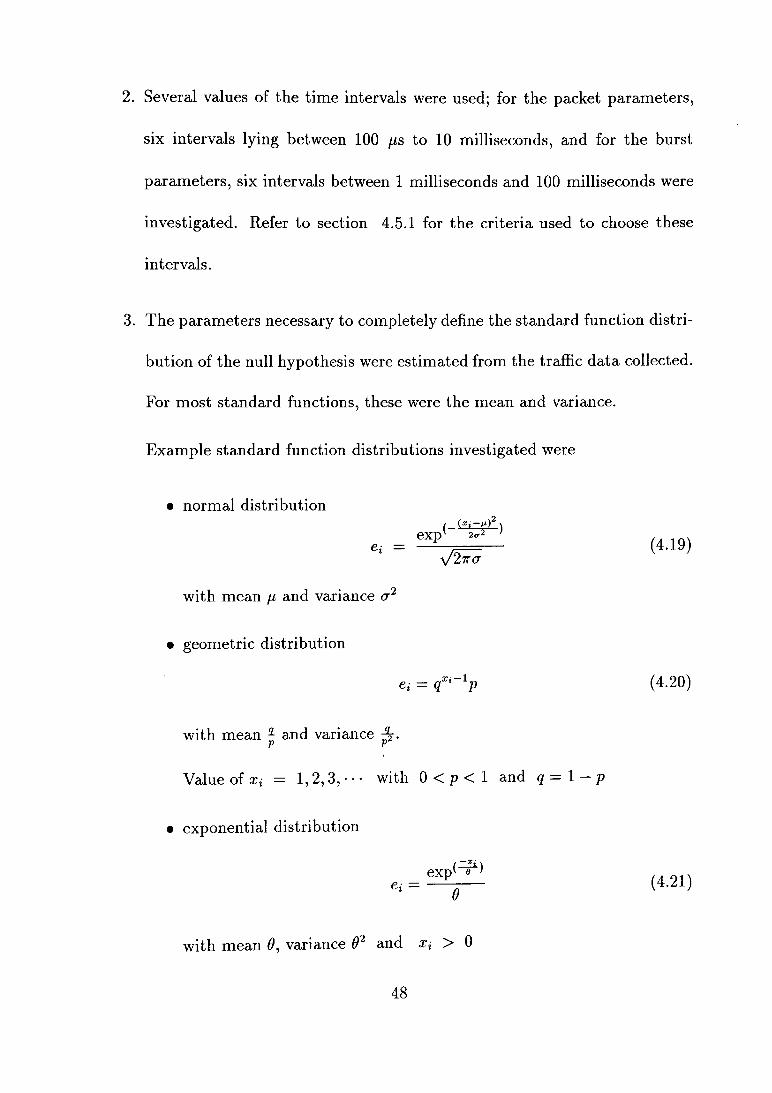
1. Data arrival distribution in time

2. the number of packets per arrival burst segment and the number of packets

per departure burst segment. These are the burst lengths.

3. packet sizes i.e. the number of bytes per departure packet and the number

38

of bytes per arrival packet.

4. the arrival inter-packet time represents the difference between the time at

the end of the receipt of one arrival packet and the time at the start of the

next arrival packet. Where the time difference is smaller than the threshold

(42.086ms above) it is defined as the packet inter arrival time interval. The

burst interarrival time interval is the interval where the time difference is

greater than the threshold.

The departure inter-packet time represents the time difference as defined for

the arrival packets, but between two consecutive departure traffic packets.

The burst interdeparture time interval is similarly defined.

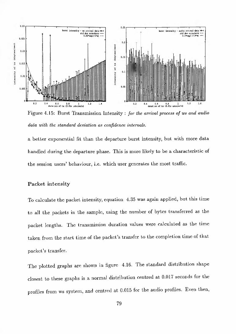
5. The transmission intensity for a packet is the ratio of the packet size to the

effective transmission time. The burst intensity is the ratio of the sum of

packet sizes of all the packets in that traffic burst to the duration of that

traffic burst.

6 . user response time is the time between the end of an arrival traffic burst

and the start of an adjacent departure traffic burst. This marks the user’s

response time to the requests received from the session, or may indicate the

start of a user’s request.

7 . idle time is the time between the end of the departure traffic burst and

the start of an adjacent arrival traffic. Idle time can represent the session’s

39

response time to the user’s transmitted requests, a display update event or

the start of another user’s response.

Figure 4.2: System data model:

a is the arrival packet, d the departure packet, and connect marks the point of connection

The idle time and the user response times constitute the inter-burst time intervals.

From the above definitions, the inter-packet time regardless of source would be a

combination of the idle and user response times, which describe the time between

packets from different sources, and the packet interarrival and interdeparture

times, each of which refers to traffic from the same source.

Note that these random variables are dependent on the users involved. In partic

ular, the number of packets per arrival burst (burst length) will be very large if

the users trade images, as occurs when running slide shows or dumping images

on the common window. The time intervals between data transfers will increase

with network loading, as the system takes longer to obtain idle conditions on

ethernet.

40

4.1.3 Parameter choices

The following parameters were chosen to describe the random variables.

• mean value showing the central value of the distribution.

• variance which indicates the spread of the values from the mean.

• squared coefficient of variation, used in relation to the interarrival time

intervals, to describe the burstiness of the traffic arrival process.

Mean

The mean represents the average value of the random variables, Xi and is cal

culated experimentally as Xi weighted by the corresponding probability density

value. For example in interarrival time data, if N{ represents the number of

arrivals within interval x,-, then the mean is defined as in equation 4.3.

mx =sum of observed values

NN\Xi -f- N2X2 + • • * T N{X{

(4.3)

NK N - w —

- f-r 'Nt = lK

= J 2 x iPx (xi)i—1

(4.4)

(4.5)

In equations 4.4 and 4.5 N is the total number of arrivals, K the number of

time intervals and Px{x%) is the probability density. Equation 4.5 is found by

letting N tend to infinity in the frequency formula, Ni/N, so that the frequency

41

becomes

P (X = Xi) = P x(x i)

Variance

A measurement of how much an individual observed value deviates from another

gives information on the spread of the sample. The standard deviation measures

the spread of the observed values, in relation to the mean value. It is found as

the positive square root of the variance, a 2. For a whole population, the variance

is obtained by first squaring the deviations from mean, and then averaging the

squares, an equivalent of a mathematical expectation E (x) of the random variable

( X —jj,)2 measured in squared units. This is represented by the following equations

«r2 = E [ { X - , i f }

N

= n)2P x(xi)i

= (4-6)i

Variance therefore measures the spread as the average of the deviation of the

random variable x from the mean. Xi is the ith observation and N is the population

size. The larger the variability the less predictable the statistic is. The variance

of the sum of the random variables can also be calculated using the following

var(X) = E [X 2] - (E [X })2 (4.7)

with var(x) representing the variance of random variable x. Hence for vector X

42

with Xi, i = 1 , 2 ,3,• • •

var(xi + £ 2 + * * *) = var(a:1) + var(£2) + • • • — 2cov(a:1:c2) — • • • (4.8)

where cov(:ri:r2) refers to the autocovariance between random variables X\ and

x 2 of the vector X .

For independent random variables, the covariance terms in equation 4 .8 will

be zero making the variance of the sum of independent random variables equal

to the sum of the variance of each random variable. The variance grows as

more random variables are added to the sum, because there will be no cancelling

effect occurring. It is possible to use this effect to test for independence between

random variables. The derivations given so far, for the variance, refer to the

situation where a whole statistical population is considered. For a sample of the

data, the sample variance s2 is calculated in the same way but by substituting

the sample mean, xm, in place of // and the value {sample size — 1 ), in place of

the population size.

1 NS = N _ . YJ,Xi - x mf (4.9)

i

Squared Coefficient of variation

Also referred to as the index o f dispersion (IDI) [Habib 92], [Sriram 86], the squared

coefficient o f variation is used to look at the relationships among successive

interarrival times. It has been shown [Sriram 86] that the complexity o f the arrival

process is represented by a high value o f burstiness. Unlike the original definition,

the yfl1 sequence o f in-

43

terarrival times is defined as { X {k, i > 1 }, a stationary process, then the sum

of the inter arrival times, Sk = X ik + X 2k + + • • • + Xik for i consecutive

interarrival time intervals in any kth sequence. Then the squared coefficient of

variation or IDI is

with

IDI = ( 4 , k > 1 } (4.10)

k°sk(E [sk]y

kcrsk(kE [X lk]y

<7 Sk

k(E [X lk])2

(4.11)

(4.12)

The square of the mean serves to normalize the cumulative covariances. Normal

ization makes the SCOV for the poisson process equal 1. This fact is used in

defining the burstiness of a process, where the deviation of a process’ coefficient

from that of the poisson process, measures the degree of burstiness. The denomi

nator in equation 4.11 above is generated using the assumption that the random

variables X ik are stationary. This gives the following relationship

E[Xik] — E [X 2k\ — ••• E[Xik] — kE[Xik] (4-13)

The variance of Sk can be calculated using the following equation

a sk — cov(Xifc, Xik) + • • * + cov(X^, Xik) + • • • + 2cov(Xik, Xjk) + • • • (4.14)

for any j ^ i. The covariance function, cov(), is defined in appendix D.

44

Using the assumption that the random variables are stationary, the following

equations result :

cov^Xjk, X jk) — cov(Xr2/c, Xu*} (4.15)

and

cov(X ^, X(i+m)k) cov(X£jj., (4.16)

for any z, j , or m so the covariance depends only on the time difference(m)

between the random variables. Substituting these equations to equation 4.14,

the variance of Sk simplifies to

k - i

aSk = kcov(X ik,X lk) + 2 ^ 2 (k - j )co v (X lk, X (1+j)k) (4.17)3=1

From equation 4.17, the variance of the sum of time intervals is dependent on the

autocorrelation/autocovariance functions. Therefore this variance describes the

arrival process indicating how the random variables relate to each other.

In this research, the variance of Sk was calculated using the equation below

adapted from [Sriram 8 6 ]

i N k i k = N k

°su = T £ S 2 - ( J - E ifc)1 (4.18)Nk k=1 X k k=1

where

Sk = ^100A:-99 + *^100A:— 98 + ’ * ‘ + ̂ lOOfc+i'-lOO + * * * + ̂ lOOA;

for a sequence of interarrival times of length 100. To calculate the SCOV, equation

4.18 was then substituted in equation 4.12 with the value of the mean calculated

as in section 4.1.3.

45

Thus c\ measures the cumulative covariance over k consecutive blocks of interar

rival time intervals. This models the cumulative effect of small individual covari

ances which may result in large packet delays. Delays in this case refer to time

taken to reach the statistics collection ports. As relevant covariances depend on

the traffic intensity, it follows that the ID I will depend on the traffic intensity.

High values of cj. indicate a high burstiness.

The length of each kth sequence of interarrival times was arbitrary chosen to

be 100 first, i.e. each kth sequence consisting of {A -̂, i > 1 < 1 0 0 } interarrival

intervals. Other investigated block lengths were 50 and 3000. The resulting values

of the SCOV were found to be in the same orders of magnitude, even though the

lengths of blocks had increased.

4.2 Data Treatment Methods

This section describes the group of tests that were applied to the collected traffic

statistics. The Chi-square goodness of fit test was used to find out how closely the

frequency distributions fitted a standard function. The Log Histogram method

was an optional test which could have been carried out to further verify the curve

fitting. To test for independence among time interval data, the chi-square test

for independence was carried out.

46

4.2.1 Chi-square goodness of fit tests

In searching for standard function forms, to describe the obtained data’s random

variables, chi-square goodness of fit tests [Strait 83] were performed. These were

used to investigate how standard functions like the exponential distribution for

continuous random variables and the geometric distribution for discrete random

variables, described the obtained data.

The random variables used to investigate the decision rules, are referred to in the

following section as the test statistics. These are the variables discussed in the

previous section.

The goal of the chi-square goodness of fit test was to test the null hypothesis that

the test statistics’ distributions fitted a chosen standard function distribution.

Below are the steps followed in the investigation.

1. Histograms were created for the parameter time series and the y axis value

fi calculated as follows depending on the parameter being considered:

• the number of interarrival time values falling into a time interval, in

the case of inter arrival time intervals.

• the number of bytes transferred at a particular time value, in the case

of arrival data.

• the average transmission intensity for a time interval, in the case of

the duration of transmission.

47

2 . Several values of the time intervals were used; for the packet parameters,

six intervals lying between 100 fis to 10 milliseconds, and for the burst

parameters, six intervals between 1 milliseconds and 100 milliseconds were

investigated. Refer to section 4.5.1 for the criteria used to choose these

intervals.

3. The parameters necessary to completely define the standard function distri

bution of the null hypothesis were estimated from the traffic data collected.

For most standard functions, these were the mean and variance.

Example standard function distributions investigated were

normal distribution

e,: =/_ (xi ~M)eXpV 2<r2V2 7T<7

(4.19)

with mean p and variance cr'

geometric distribution

Q = qXi 1P (4.20)

with mean 1 and variance p p

Value of X{ = 1,2,3, ••• with 0 < p < l and q = l - p

exponential distribution

e,; =expv o t (4.21)

with mean 9, variance 62 and Xi > 0

48

Note that, et- is the expected frequency and X{ is the value of the ith time

interval. The mean and variance were taken from the variables’ graphs.

4. With fi as the observed frequency (i.e. the probability density function from

the graphs) and the expected frequency calculated from the standard

function distributions given in step 2 ; a graph of fi and e* on the same time

series is then plotted.

5. : x 2 was then computed from the following ratio

x2 = E {Ji^ - (4.22)i=1 e*

where m is the sample size, x 2 is then a random variable with chi-square

distribution and (m —t—1) degrees of freedom, t is the number of parameters

estimated from the sample in order to define the chosen standard function

distribution, e.g.for the normal distribution, t equals 2 counting fi and a.

6 . The value of i was looked up from tables of x 2 distribution with

a as the level of significance which indicates the error of rejecting the null

hypothesis given the null hypothesis is true. The null hypothesis is rejected

if

x2 > X2, ^ - ! (4.23)

The results for the chi-square goodness of fit tests are tabulated in table 4.1, for

those distributions which closely resembled the negative exponential distribution.

49

The values o f A and B are coefficients o f the fitting curve

et(z) = A * exp^-1*5*2̂ (4.24)

which can be rearranged to give the following equation

e{(x ) = K * Aexp^***)

where A is the mean value and K a scaling constant. The results show that the

random variable distributions were closely described by the fitting curves. This

is indicated by the small chi-square values.

4.2.2 Log Histogram method

Looking at the two functions that were nearer the shape of the data, i.e. the

geometric and the negative exponential, it is possible to get a linear relationship

after taking the logarithm of the distribution equation. This test is carried out to

investigate the possibility of piecewise linearity in the observed data which would

indicate the desirable compound Poisson arrival process or otherwise.

• For the geometric distribution, taking logarithms of the distribution func-

tion gives the equation

log ei = log p + (x{ - 1) log q (4.25)

= log q T (log p log <7) (4.26)

which is a straight line graph of gradient log q

50

Table 4.1: Chi-square goodness of fit tests. The chi-square values are for those ran

dom variable distributions which resemble the negative exponential distribution. A and

B are the coefficients of equation 4-%4 the figure dep.= departure data, arr.=arrival

data, wsa=ws arrivals, wsd=ws departures, where marked *, the curve is defined by two

exponential functions. The number in brackets is the coefficient of the second exponen

tial curve.

variable A B X2 deg.of freedom

burst length-audio dep. 0.4 0.4 0.8197 16

burst length-ws dep. 1.0 0.7 0.1878 16

burst length-audio arr. 0.4 0.4 0.8197 16

burst length-ws arr. 1.0 0.7 0.1193 16

Interdepartures-mike 0 .2 (0 .1)* 8(17)* 1.6136 146

Interdepartures-ws 0.12 10 0.069 146

Interarri vals-speaker 0.3 16 0.4051 146

Interarrivals-ws 0.13 10 0.0671 146

Intensity-mike 0.3 3.5 3.7289 146

Intensity-wsa 0.01 5 1.3687 146

Intensity-speaker 0.1 2.5 6.8618 146

Intensity-wsd 0.1 10 18.405 146

Idle time-audio 0.1 13 0.2629 146

Idle time-ws 0.8 80 0.6418 146

User response time-audio 0.08 12.5£ 1 ______

0.0828 146

User response time-ws 0.6 60 0.7726 146

Table 4.2. Contingency Table : for iid tests. The figures are taken from the packet

interarrival times for the ws application

Observed values /„■ Expected values ez-

set(l) set(2 ) row sum set(l) set(2 ) row sum

2.215 2.084 4.299 0.98901 3.30999 4.299

23.905 91.741 115.646 26.60514. 89.04086 115.646

1.95 2.023 3.973 0.91402 3.05898 3.973

140.756 344.708 485.464 111.68426 373.77974 485.464

2.004 131.170 133.174 30.63757 102.53643 133.174

column sum 170.83 571.726 742.556 170.83 571.726 742.556

• For the exponential distribution, taking logarithms gives the equation

lo9‘ e' = (4'27)

again a straight line but with gradient — 1/0

Thus a log histogram with piecewise linear segments may indicate a combined

Poisson process. This test was not carried out owing to the desirably low values

in the chi-square goodness of fit tests.

4.2.3 Independence (iid) tests

To establish if a sequence of random variables (interarrival times in this instance) are

independent generally requires more than just testing the independence o f

consecutive pairs. The IDI for example would be ideal for this purpose [Sriram 86].

However, due to time and processing constraints we were only able to test the

independence o f pairs o f variables in this thesis. The chi-square test for

independence was used [Lapin 90]. iid refers to independent and identically

52

distributed random variables. Below are the steps followed to perform the test

1. The chi-square statistic was used to test the null hypothesis that two sets

of random variables were independent.

2. A significance level was then selected for this decision rule. This value, as

in the goodness of fit tests, gives the probability o f miss, the chances of

rejecting the null hypothesis given that it is true.

3. The two sets of the random variables were then set up in a contingency table

(Table 4.2) which uses figures taken from the inerarrival time intervals for

the ws program. From this table,

• set(l) = {2.215, 23.905, 1.95, 140.756, 2.004} and

• set(2) = {2.084, 91.741, 2.023, 344.708, 131.170}

The null hypothesis then was that the value of a random variable in one

set was independent of which set was chosen. These observed values were

denoted as /¿. The sets were first chosen as follows:

set(l) consisted of the first, third, fifth, etc i.e. odd numbered observations

set(2) consisted of the second, fourth, sixth etc i.e. even numbered obser

vations

Then the sets were chosen as groups of non-overlapping intervals.

53

4. The expected values of the random variables if the null hypothesis was true

were calculated by keeping the totals of the columns and rows in the contin

gency table constant. The expected random variables were then calculated

as the product of the row sum and the column sum divided by the total

sum of all the rows and columns.

For instance, the expected value of row 1 and set(l) is

en 2.299 *170.83

742.556

5. The random variable %2, representing the test for independence, was calcu

lated as

x 2 =1 EE ( f i j e i j)

total row sum . etî-i 3 J(4.28)

6. A decision was made after looking up the chi-square value in the tables using

the chosen level of significance (step 2 above) and the number of degrees of

freedom. The number of degrees of freedom are calculated as

(number of rows — 1) (number of columns — 1)

The hypothesis was rejected if the calculated chi-square value was the

greater of the two. In that case it meant that the random variables were

not independent.

On applying the test, the results indicated that the packet interarrival time in

tervals were not indépendant of each other. The calculated chi-square values are

54

Table 4.3: Chi-square test for independence.

The chi-square values are for groups of non-overlapping time intervals, averaged over

all the runs.

threshold y 2 value 43.773 at significance level 0.05

random x 2 X2 degrees

variable for bursts for packets of freedom

Interdeparture time - ws 1.2535 127.69 32

Interarrival time - ws 7.806 158.22 32

Interdeparture time - audio 1.2148 4891.44 32

Interarrival time - audio 3.1519 23.56 32

Interdeparture time - ws/audio 5500 26000 32

Interarrival time - ws/audio 1322 70000 32

displayed in table 4.3. This figure also shows that the burst interarrival time

intervals were independent of each other for separately considered audio and ws

data traffic.

4.3 System Environment

The application programs were executed on an Ethernet network, at the Uni

versity of Wollongong’s electrical and computer engineering(ECE) department.

Figure 4.3 gives a simplified layout of the network configuration. The network

55

operates at 10Mbits/s connecting over 6000 computers, with about a 100 of them

in the ECE. The network carries IP, Novell and ethertalk traffic. The experiments

were performed using T C P/IP and UDP/IP protocol stacks.

Two configurations of the Collaborative Work system were used in the collection

of data.

The first configuration involved computer terminals on the same network(elec.uow.edu.au)

carrying normal load i.e. about 1 M b/s on average as determined by displaying

the ethernet traffic. These terminals were located in the Postgraduate Computer

Laboratory (35G46).

Next the sessions were run between terminals again on the same LAN but located

in different Labs with a round trip delay of 2ms (i.e. between the 4th Year Thesis

Lab and 35G46). A session in this project refers to the execution of the conference

application programs described in Chapter 3.

The second configuration involved workstations on different local area networks.

The networks involved were the computer science department s (cs.uow.edu.au)LAN

and the Switched Networks Research Centre’s LAN(snrc.uow.edu.au). The route

to these networks is shown in figure 4.3.

Both two and three terminals per session configurations were used. Participants

were volunteers who were given roles to play whilst the control program recorded

the statistics. A variety of situations were enacted including .

56

1. a meeting between directors discussing the management structure of their

new company.

2. architects discussing building plans.

3. telecommunications engineers planning for a local area network.

4. A lecturer and his student discussing a research topic.

Role-play was chosen because it gave us control on when the sessions took place

and on the topics discussed. That way it was possible to analyse data arising from

a variety of situations. For instance, scenerio 1 would generate more collaborative

data the audio due to a lot of sketching, whereas scenerio 4 above may result in

more audio data transfer in one direction than the other.

Figure 4.3: The Local Area Network diagram

57

4.4 Data collection

Data was collected at the ports of the WS server terminal through the use of a

control program that traced the system calls occurring during the running of the

collaborative work system.

Usually programs monitoring data look at the packets passing through the net

work and extract the address and packet length information. In this investigation,

statistics were collected at the application layer interface. In the case of the trans

mitted data, statistics were collected before the data was encapsulated with the

address and header information. For the case of the received data, this was after

the data had been demultiplexed or stripped of the packet header information.

Figure 4.4 shows the structure of the data collection mechanism. Our concern

was for traffic profiles generated by our particular user process. By modelling it

at the operating system interface, it would then be independent of the layers be

low as long as they can supply the required characteristics at the interface to the

user process layer. It would then be possible to substitute the lower layers by any

network protocol stack and expect to observe the same application behaviour. A

brief description of the Unix operating system is given below.

4.4.1 Unix networking

Unix supports T C P /IP which is accessed by specific system calls. For instance,

connect initiates a connection with a remote socket, send sends a message through

58

a given socket and recv receives a message on a given socket [Tanenbaum 88]. The

sockets in Unix are the end points to which connections can be made from the

operating system and to which processes can be attached from the user appli

cations layer. When a receiving socket is created, it is bound to a name and

allocated buffer space for storing incoming connection requests. To receive a re

quest, a new socket is created and used for that connection, leaving the first, (the

bound) socket free to receive more connection requests. The TCP layer accepts

long packets from the user process and breaks them down into datagrams to be

transmitted through the IP layer. The TCP layer is responsible for time out,

retransmissions, reassembly and error control of the transmitted datagrams. The

IP layer provides connectionless service and attaches header information to the

datagrams before forwarding them to ethernet.

The control program used in collecting data was a modified version of the strace

program from Erasmus University Rotterdam. By configuring this program to

time-stamp each system call at the start, and at the end of the system call, it was

possible to extract the received and the transmitted data information, including

the effective duration of transmission. These time values and the amount of

data units sent, were then used to calculate data transmission variables like the

intensity of transmission or the interarrival time intervals.

A total of 9 runs were carried out during September 1993 resulting in a total of

4 hours session time and 171529 packets handled. From this data, the series of

59

| d a t a |

[ d a t a ]

| T H | d a t a )

_______ I_________| D H | N H | T H |d a t a ~ 1

Figure 4.4: Strace: control program for data collection

values of the random variables of the assumed model were calculated.

4.5 Data treatment

In the analyses, raw data was arranged in a series of adjacent blocks or class

intervals [Lapin 90] with the class frequency calculated as the number of obser

vations of a particular variable falling into that class interval, e.g. frequency of

occurrence of the interarrival time intervals. Histograms were drawn with the

class frequency on the y-axis and the time intervals on the x-axis. Impulses of

height equal to the class frequency were used in the histograms.

Figure 4.8 is an example of a histogram relating the relative frequency to the

number of packets per each burst. For example, from that graph, the percentage

of traffic bursts found with a length of 2 packets was 20% for ws arrival data and

25% for the audio arrival data.

Attempts were then made to categorize the obtained shape of the frequency dis-

60

tribution with known standard distributions like the geometrical and the negative

exponential. The assumption was that the rough shape resulting from this sam

ple data would be an estimate of the smoother frequency curve that might result

if an infinitely large sample was used.

4.5.1 Choosing interval width

As the determination of the width of time intervals is crucial to the description

of the frequency distribution, several intervals were tested, namely the following

- 100//S, 5ms, 50ms, 100ms, and 500ms. The choice was then based on the

compromise between the interval having too much detail or too little as to be

detrimental to the shape of the distribution function. Too small an interval

(100//S width) resulted in jagged, difficult to describe plots and an interval width

greater than 0.2 seconds tended to miss important frequency pattern information.

The interval giving the most distinct shape of the frequency was found at 1ms

interval width for the packet distribution and 10ms width for the burst segment

distribution. This result is intuitive as the bursts behaviour of the traffic is at

a greater time scale than the packet traffic. Equal length interval widths were

adopted for simpler interpretation.

61

rela

tive

fr

eque

ncy

4.5.2 Relative frequencies

In order to easily adapt the frequency curves to traffic data, of different sam

ple sizes, and which may have been obtained under different conditions, relative

frequencies were used in all the graphs. These were calculated by dividing each

class frequency by the total sample size ( - the sum of all the class frequencies).

The graphs would then display the relative frequency distribution or the proba

bility density function. This presentation makes it easier to compare the graph

characteristics with other similar applications. Real quantities do not convey the

plotted value’s relationship to the total. For instance, knowing that 50% of the

data is transferred within 0.02s conveys a lot more information than being told

that 5000 bytes are transferred within 0.02s.

i0.9

0.8

0.7

o . e

0.5

0.4

0.3

0.2

0.1

0«.0 1 2 3 4 5

time intervals

Figure 4.5: Cumulative frequency distribution to find the time interval upper

limit

62

4.5.3 The upper limit

To find the upper limit for the time intervals, a cumulative frequency distribution

(similar to figure 4.5) was used with the x - axis time intervals stretching up to

the highest calculated time interval (i.e highest observed value). This was done

by adding each class frequency to the sum of the lower class frequencies, hence

giving information on the level of the class intervals. The upper limit was then

taken to be the interval below which 95% of the frequency data falls. The upper

limit gives the limit beyond which the obtained data no longer behaves typically

and is an insignificant proportion of the data.

4.5.4 Confidence Interval

The confidence interval defines the precision and the reliability of the obtained

data. Reliability refers to the probability that the estimate is correct; and preci

sion is the probability that the estimate is close to the target parameter. In the

random variables investigated, both the y-min/y-max values and the standard

deviation were used as confidence intervals. The y-min and y-max values were

found from the averaging of the histograms obtained for each test session run.

The standard deviation value was calculated as in the definition given in section

4.1.3.

Standard distribution functions to fit the variables of the traffic model were then

investigated from this data.

63

4.6 Data Analysis

This section reports results obtained during session experiments, and discusses

the interpretation of the results in terms of the analysed variables.

4.6.1 Arrival packets

Figure 4.6 shows graphs of the distribution of the arrival and departure processes.

The graphs indicate the similarities of the obtained profiles with the assumed data

model of section 4.1.2. As in the model of figure 4.2, the graphs show multiple

arrivals and departures confirming the theory of batch arrivals (burst segments).

They also show burst segments in which the packets within the segment have dif

ferent lengths (-randomly varying packet sizes). Note that the inter-packet times

and the inter-burst times have varying lengths. These intervals are discussed in

detail in section 4.6.4.

“ T-----------1----------- 1-----------vs packet arrivals -

1 ' j

ws acket depart ires - 2000 i

1800 ■ j

- 1600 -

1400 - i

■1200 ■ i

1000

800

_i____

audio packet arrijalsl audio packet departijires(

883.2 883.4 883.6 883.8140.12 140.14 140.16 140.18 140.2 140.22 140.24 140.26 140.28 140.3 883

Figure 4.6: Comparison between arrival and transmitted data

64

pack

et le

ngth

(b

ytea

)

The graphs in figure 4.7 shows that most of the data handled has packet lengths

that are less than 5000 bytes with only a few having the maximum of 8000

bytes length. There is therefore a possibility of trading-in the bandwidth of the

transmission equipment, to a little degradation in system performance. This could

be done by allowing a bandwidth of just half that of the peak traffic handled. A

possible situation might be the running of two sessions where only one session

was fully allowed for. This assumes that the two sessions do not carry peak traffic

at the same time. If they do, the result may be an increase in waiting or response

times, as the processes wait their turn to transmit.

Figure 4.7: Typical transfer data: combined ws and mike

Similar traffic patterns were obtained for both the sessions run within the same

local area network and those run across separate local area networks. The data

collected from the two configurations, was therefore combined in the analysis to

improve the confidence intervals.

65

Graphs for the arrival processes of the ws application and the audio communi

cations when considered separately are displayed in the appendix (figure A .l).

The graph from the audio application shows an almost constant packet length,

for the arrival data collected by speaker program, of around 1048 bytes whilst

the ws program exhibits large variations of packet length, with a minimum of

8 bytes. Comparing with the graphs in the appendix for the transmitted data,

(figure A .2), it is clear that the largest volume of data is generated by the audio

communication program, and thus has a greater influence on the CSCW system’s

overall traffic characteristics.

4.6.2 Burst length

The burst length refers to the number of packets within each burst segment.

This value was obtained by keeping track of the number of adjacent interarrival

time intervals whose value was less than the threshold of 42.086 ms. Whenever

the calculated intervals were greater than the threshold value, this was recorded

as the start of a new burst segment and hence the end of the previous burst

segment. The results, displayed in figure 4.8, show the burst length calculated

using arrival data from the audio and from the ws application. Graphs from the

departure data for each application are shown in the appendix (figure A .3).

From the graphs in figure 4.8, the number of packets per burst segment for both

received and transmitted data showed an exponential distribution with a mean

66

rela

tive

fr

eque

ncy

0.6

0.5

0.3

00 5 10 15 2 0 2 5 30 35 4 0 4 5

Humber o f packets

0.4

0.35

0.3

ug 0.25

&8* 0.2•>-HV

h 0.15•

0.1

0.05

00 5 10 15 20

Number o f packets

Figure 4.8: Burst Length : arrival data for ws and audio processes

value (parameter 9) of 1.429(=l/0.7) for ws data and 2.5 (=1/0.4) for audio.

The negative exponential curve, from figure 4.8, is given by the equation

f (x i ) = exp {-xi /&)

= exp {-0.1 x i )

(valid for 1 <= xi <= 12) (4.29)

the integral o f this empirical density function is approximated by the sum o f the

function between given limits with interval 1, i.e., X / f e ) = 0.988.

Hence the mean is 1.429 packets per burst segment for WS collaborative work

system and 2.5 packets per traffic burst for the audio communication programs. A

small mean value indicates that it is difficult to predict when the next packet is

going to come given that one packet has already been transferred.

Extremes, like 12 packets per burst segment, occurred when images were

transferred between displays, and in some cases, in the audio application programs.

67

4.6.3 Packet sizes

Another important parameter in network design and analysis is the distribution of

the size of the packets handled. By looking at the number of packets of the same

size, the average number of data units per packet was found. When the audio

system was considered on it’s own (figure 4.9), almost 99% of the packets had

a packet size of 1048 bytes, with some received audio packets deviating to 8000

data units in extreme cases. For the WS data system, the packet size distribution

for arrival data showed about 95% of packets with a packet length of 32 bytes.

This brought the average packet size to about 100 bytes per packet because of the

extremes of around 4000 bytes. The data displayed in the appendix (figure A .5)

gives the distribution of the packet sizes for the combined application programs.

The graphs show two prominent peaks, one at 32 bytes and another at 1048

bytes. This graph (figure A .5) indicates a random distribution. The first peak

in figure A .5 therefore indicates the activities of the cursor movement in the WS

application. The peak at 1048 bytes in the same graph is influenced by the audio

communication. This raises the overall mean of the packet sizes to nearly 800

bytes.

The high relative frequency values in figure 4.9 suggest that the arrival process

may be deterministic, consisting of only two packet sizes, 32 bytes and 1048 bytes.

These values are vital in simulation work where they can be used to characterise

the size and distribution of arrival packets. Another application of this parameter

68

lati

vo f

requ

ency

Figure 4.9: Packet size Distribution : arrival data ws and audio processes

would be to compare the largest sized packets with the average packet size, thus

get a feel of how effectively the CSCW system utilizes the network. This can

then be used to make decisions on how to design and dimension the network.

4.6.4 Interarrival intervals

The sequence of interarrival times is a superposition of the packet processing

and transmission times [Forys 90]. As in the previous analyses, raw data was

arranged in a series of adjacent class intervals with the class frequency calculated

as the number of interarrival time intervals falling into that interval. The interval

widths used were 1ms for the packet interarrival distribution and 10 ms for the

burst interarrival distribution. These values, determined empirically, were found

to give a better and more distinct distribution than the other investigated values

(section 4.5.1). In network analysers, the interarrival times, together with service

69

rela

tive

fr

eque

ncy

time data parameters, are used to estimate network response times [Forys 90].

0.1 0.2 0.3 0.4 0.5 0.6 0.7 0.8 0.9 1time interval (0.01s intervals)

Figure 4.10: Burst Interarrival time distribution for audio and ws processes showing

best fit negative exponential curve and standard deviation confidence intervals.

Burst interarrival times

For the burst interarrival time intervals, the vector of the time intervals was found

as the length of time from the completion time of the last packet of one burst to

the start of the first packet of the next burst segment; or simply the interarrival

time intervals which were greater than the threshold value of 42.086 ms. The

latter calculation method was used in this analysis.

The mean and variance for the interarrival time intervals were calculated and the

chi-square goodness of fit tests showed an approximation towards the negative

exponential distribution. The graphs, figures 4.10 and 4.11, show a mean of

between 0.1 seconds (1/10) and 0.0625 seconds (1/16) for ws and for the audio

traffic respectively. This suggests that the burst segments arrive within 62.5 ms

70

rela

tivo

fr

oquo

ncy

to 100 ms of each other on average, with a variance of 0.3% to 1%. The curves

from the audio program, figure 4.11 show a larger deviation from the negative

exponential. The graph of the interdeparture time interval from the mike program

indicates a possibility of being modelled as a sum of two exponential functions;

one centred at zero and of mean 0.0588 seconds, and the other centred at 0.25

seconds with a mean of 0.125 seconds.

“ I----------- 1----------- 1----------- 1----------- 1----------- 1----------- 1----------- 1----------- 1-----------; burst interdeparture - audio transmitted data t4-i: std dev errorbars -----'■ 0.2*exp(-8*x) -----

0.12 ----- 1----------- 1----------- 1----------- 1----------- 1----------- 1----------- 1----------- 1------------1-----------burst interdeparture - vs transmitted data t4—t

std dev errorbars -----0.12*eip(-10*x) -----

0.1*exp(-17*x) ----- '0.1

' \ •

> 0.08c•

s]

\■ \ ■

u 0.06 •>li

\ '

ttl

__1__

___

! 0.04

, ,,

0.02

00.1 0.2 0.3 0.4 0.5 0.6 0.7 0.8 0.9 1 0.1 0.2 0.3 0.4 0.5 0.6 0.7 0.8 0.9 1

time interval (0.01s intervals) time interval (0.01s intervals)

Figure 4.11: Burst Interdeparture time distribution for audio and ws processes

showing best fit negative exponential curve and standard deviation confidence intervals.

f(Xi) = fi{Xi) + f 2(Xi) (4.30)

with

f l ( x i ) = 0.1 exp‘ ^ x/ for 0 < jc/ <= 0.25 (4.31)

and

f l ( x i ) = 0.2 exp("^Xi ) (valid for x[ > 0.25)

the integral o f these empirical density functions is approximated by the sum o f the

functions between the given limits using an interval o f 0.01.

71

rela

tive

fr

eque

ncy

= 0.1 exp*"8**-“ 0'25)

0.07

0.06

0.05

0.04

0.03

0.02

0.01

00 0.005 0.01 0.015 0.02 0.025 0.03 0.035 0.04 0.045 0 0.005 0.01 0.015 0.02 0.025 0.03 0.035 0.04 0.045

time intervals(0.001s in tervals) time intervals(0.001s in tervals)

Figure 4.12: Packet Interarrival time distribution :audio and ws processes with the

standard deviation used for confidence intervals

Packet interarrival times

To analyse the packet interarrival time distribution, a statistical treatment was

used that was similar to the burst interarrival time treatment. The graph for

the combined ws and audio traffic data (figure 4.13) shows two peaks, one at

0.0195 seconds and another at 0.0355 seconds, with the rest of the class frequencies

scattered below the 2% value. This same pattern is indicated in the traffic profiles

from the arrival audio data (figure 4.12). As in the profiles from mike, the

distribution can be modelled as two normal distribution curves with means 0.0195

and 0.0355 seconds (equations 4.32 to 4.34).

f ( x i) = f i { x i) + f2(x i) (4.32)

1 J 1 i “ i i i----------- i---------- 0.25 —,--- - ---------1-----------1---------packet in te rarr iv a ls - ws a r r iv a l data ►♦h Backet in te rarr iv a ls - audio a rr iv a ls >4-i

\std dev errorbars ---- std dev errorbars ----

\ 0.2 . Ît si\ > iI

i j \ 0

1 1, l 'i 0-159M•H t

1 ï i \ i \ 9J i i . >! a 0.1J H9 1* v / W Ì \ 1 w 1

i U\ Ì i ■

\ h i1

'4 ;

W !0.05

! \ \A ! !

V n----1-----------» » » 4.1______ 1______ ■ ■ i t t 0

ï

t 't > 11 t 't 111-*1*-*-!__

72

rela

tive

fr

eque

ncy

with

fl(xi) =exp

, ( x ; - 0 . 0 1 9 5 ) 2 xV o„2 )

and

fiixi) =exp

y/2TTO\

l ( x v —0 .0 3 5 5 ) 2 \

(4.33)

(4.34)\/27r~o~2

The interdeparture time intervals for the combined traffic data and from mike

were different showing a high spread (almost uniform distribution) of values from

about 0.01 seconds to 0.045 seconds. This trend was also evident in the traffic

profiles obtained from the ws arrival and departure data.

1 1 1 1 1packet interdeparture

---------1------------ 1------------1------------audio transmitted data •

std dev errorbars-----

| .

• ♦ .

!!• I

!

\ \ 'i |1 M .

A t ! \ !\ 1 \f \ / \ / V / \j \ 1 \

l U i v .

i — i------------1------------1------------1------------1------------ 1------------1------------packet interdeparture - ws transmitted data t4—l

spd dev errorbars -----

\ \ ‘i \

j 4

♦ f\ k I \] i \ A y \ i \

- 1 ¡ i f 1 ] / d f \ .

\ j i V 1i f i "

A______ ¿ w ■________1________1________1________1------------1-----

0 0.005 0.01 0.015 0.02 0.025 0.03 0.035 0.04 0.045time intervals(0.001s intervals)

0.005 0.01 0.015 0.02time intervals (0.

0.025 0.03 0.035 0.04 0.045001s intervals)

Figure 4.13: Packet Interdeparture time distribution for audio and ws processes

with the standard deviation used for confidence intervals

The ratio of audio arrival data to ws arrival data was about 4 to 1, with a

similar ratio applicable to the departure data. This could be the reason why the

traffic profiles from the combined audio- ws programs are similar to those from

the speaker program more than they are to the ws data traffic profiles. The audio

73

departure data did not have much impact on the combined audio -ws profiles; it

appeared that the peaks from the audio data ( mike program) coincided with the

dips in the ws traffic profiles because people were either talking or drawing and

not doing both at the same time.

Burstiness

The interarrival time intervals indicate the dependencies between data in the ar

rival process. As has been discussed before, the squared coefficient of variation[Sriram 86],

c|, looks at the covariances among successive intervals. Hence by calculating this

coefficient for the interarrival time intervals, the burstiness of the arrival data is

determined. The coefficient has been defined in section 4.1.3 as

2 _ Var[Sk]Ck ~ *(£[*,])*

where {Xk ; k > 1} are the interarrival time intervals, with Sk as the sum of

the interarrival intervals in the kth sequence. In [Sriram 86] it is shown that

cl equals c\ for all k for single or less than 20 voice sources. It is not shown

however whether this applies to any number of time intervals in a sample. The

suggestion could mean that the whole vector of interarrival time intervals is taken

as one block. When calculations of c\ were carried out using k sequences of 100

and of 50 time intervals, it was found that the collaborative work system gave

squared coefficient of variation figures that started very high, (cq 20000) and

approached a value(c^5 « 40) lower than the initial by almost three orders of

74

Table 4.4: The Squared coefficient of variation for time intervals. The sample size

is given as (packets sample size) : (bursts sample size)

Arrival data

Type Packets Bursts sample

of mean variance sqd coeff. mean variance sqd coeff. size

traffic value value of var. value value of var.

audio 0.0246 0.0006 1.0519 0.1845 0.368 29.3757 13855:2415

data 0.0209 0.0059 13.429 0.3578 0.5005 3.9088 1516:1755

comb. 0.0210 0.0006 1.4181 0.1521 0.1651 7.1339 14149:5393

Departure data

audio 0.0258 0.0034 5.1542 0.6091 0.1555 0.6091 2585:5553

data 0.0207 0.0037 8.6866 0.3326 0.4932 4.458 2376:1784

comb. 0.0217 0.0017 3.72 0.2652 0.1226 1.7427 5087:7212

magnitude, as k increased. In [Sriram 86], the k sequences used were of 3000

time intervals and gave the c\ value as starting from 18.1 and reducing towards

one as k increased. In table 4.4, this coefficient was calculated using the variance

of the whole sample.

Note, the sample size is given as (packets sample size):(bursts sample size) in

table 4.4; this table gives a summary of the parameters for the interarrival time

intervals distributions shown in the graphs displayed in this report. The squared

75

coefficient of variation is taken as the ratio of the overall variance to the square

of the overall mean for a particular application. This assumes that the entire

sample size is one kth sequence of time intervals, and hence k — 1, giving the

aquared coefficient of variation as c\

The burstiness of an arrival process is important in determining the utilization

of the network and in the allocation of network bandwidth. A higher burstiness

indicates large variations in the arrival data and hence results in the network

being under-utilized. Thus, in addition to the squared coefficient of variation,

the ratio of transmission occupation time to call duration can be used to mea

sure burstiness. The higher the value of the squared coefficient of variation, the

higher the burstiness of the variable; and the lower the ratio of occupation to call

duration, the higher the burstiness.

4.6.5 Intensity of Transmission

Here two dimensions of the statistical data are investigated namely, the rate of

transmission and the duration of transmission. The goal is to find any relationship

between the two parameters i.e. whether large volumes of data are transferred

at a higher rate or that transmission rate is constant, i.e. independent of the

amount of data handled. A scatter diagram, as in figure 4.14 gives an estimation

of the shape of the graph, showing a decrease in the rate of transmission as

the transmission time increases. In such curves, large volumes of data would be

76

inte

nsit

y of

tx

(kby

tes/

sec)

equivalent to a large duration. The intensity of transmission shows the variation

of transmission speed with the volume of data sent or received by the terminal.

The construction of the histograms for the transmission intensity curves was done

by adding up all the transmission intensities of those values of the transmission

duration that fell into a particular class interval, and then finding their average

in relation to the number of transmission duration values found. This average

intensity of transmission formed the class frequency of that particular interval.

The intensity is calculated using the following equation :

h =(no. of bytes transferred) duration of transmission

(4.35)

All the graphs in figures 4.14, 4.15 and 4.16 therefore reflect the average intensity

of transmission for time intervals.

duration o f tx (0.01s intervals)0.2 0.4 0.6 0.8 1 1.2 1.4

duration o f tx (0.01s intervals)

Figure 4.14: Burst Transmission Intensity : for combined ws and audio data using

the standard deviation as confidence intervals.

77

Burst intensity

For the burst intensity, the number of bytes transferred per burst segment, was

found as the sum of all the packet lengths of the packets within that burst seg

ment; whilst the duration of that burst segment was the total time taken from

the start of the first packet of that burst to the completion time of the last packet

of the burst segment. This burst transmission duration therefore included the

periods of inactivity between adjacent packet transfers, therefore results in lower

transmission intensities when compared with packet intensity values. The his

tograms plotted for the burst intensity in figure 4.14 show good approximations

to the negative exponential distributions, similar to those obtained for the burst

interarrival time intervals. Figure 4.15 shows plots with large values of confidence

intervals such that it is not possible to find a common distribution function to de

scribe the data. Looking at the traffic profiles for the audio data separately from

the ws system (Figure 4.15) the shape of the graphs do not show a clear expo

nential curve, exhibiting scattered values up to a transmission duration of around

1.5 seconds. It appears then that a lot of smoothing occurs on combination of

the two applications (figure 4.14), i.e. the audio and data integration.

Some of the graphs have been drawn in Appendix A with the maximum and min

imum intensity values as errorbars to indicate the range of y-axis values obtained.

The fitting exponential curves have a mean value of 0.2 for the intensity of the de

parture burst and 0.1 for the intensity of the arrival burst. The arrival burst had

78

burst intensity audio arrival data •std dev errorbars -----

0.1*exp(-2.5*x) -----

0.4 0.6 0.8 1duration o f tx (0.01s intervals)


0.2 1.21.2 1.4

Figure 4.15: Burst Transmission Intensity : for the arrival process of ws and audio

data with the standard deviation as confidence intervals.

a better exponential fit than the departure burst intensity, but with more data

handled during the departure phase. This is more likely to be a characteristic of

the session users’ behaviour, i.e. which user generates the most traffic.

Packet intensity

To calculate the packet intensity, equation 4.35 was again applied, but this time

to all the packets in the sample, using the number of bytes transferred as the

packet lengths. The transmission duration values were calculated as the time

taken from the start time of the packet’s transfer to the completion time of that

packet’s transfer.

The plotted graphs are shown in figure 4.16. The standard distribution shape

closest to these graphs is a normal distribution centred at 0.017 seconds for the

profiles from ws system, and centred at 0.015 for the audio profiles. Even then,

79

isit

y of

tx

(kby

tes/

sec)

1 1 n------------1------------ 1 i i i[ packet intensity - audio arrival data H—■

std dev errorbars -----

-

!

|

■

♦

- ♦ ■1

\

\ ........................005 0.0 1 0.015 0.02 0.025 0.0 3 0.035 0.04 0.045

duration o f tx (0.001s intervals)0 0.005 0.01 0.015 0.02 0.025 0.03 0.035 0.04 0.045


Figure 4.16: Packet Transmission Intensity : for the arrival process of ws and audio

data. Both plots have been drawn with the standard deviation as confidence intervals.

it ’s a poor approximation to the shape of the graphs. The only suggestion these

graphs project is that most of the packet data is transferred with a transmission

duration lying between 0.014 seconds and 0.02 seconds with a packet intensity

of slightly over 6 kbytes/sec. (roughly 64kbits/sec) for the audio data, and peak

packet intensity for ws data of slightly under 1 kbyte/sec ( 8kbits/sec). The

lower data rate values could be a result of discarding potential packets due to the

silence suppression employed.

4.6.6 Response times

The definitions for the idle time and the user response times have been given in

section 4.1.2, where they are described as inter-burst time intervals because they

look at the time intervals between adjacent packets from different directions, e.g.

80

rela

tivo

fre

quen

cy

0.4 1 l i------------------ 1------------------ 1------------------ 1------------------ 1------------------

id le time - combined ws i audio data >4—I0.4

user response time - combined ws & audio data >4—1

std dev errorb ars ------- std dev errorb ars ------0.35 0.4*exp(-50*x) ............ 0.35 0.4*exp(-50*x) — • .

0.3 0.3

11 >4

0.25 '1 • 1 0.25 &

20.2 - ^ 0.2

0>-H

♦ l0.15 h 0.15 l .

\9M

0.1 \ . 0.1 \V \

\ \ \0.05 v , , - 0.05 V ■

0.05 0.1 0.15 0.2 0.25 0.3 0.35 0 response time (0.01s intervals)

4 0.05 0.1 0.15 0.2 0.25 0.3 0.35 0. response time (0.01s intervals)

Figure 4.17: The user response time and idle time : for the combined ws and audio

data with the standard deviation as confidence intervals.

between the last arrival and the first departure after that arrival or vice-versa.

The values of these time intervals were obtained by keeping track of the traffic

flow direction. The graphs for the user response times and the idle times are

shown in figures 4.17, 4.18 and 4.19.

Idle times

The idle time was calculated as the inter-burst time from the end of a departure

burst to the start of an adjacent arrival burst . This response time therefore

consists of the time it takes the user response packet to be distributed among the

session participants, and the time taken by a packet generated within the session

to arrive at this same user.

The graphs shown in figures 4.17 and 4.18 show that the idle time can be

81

rela

tive

fre

quen

cy

0.8

r

—i------ i------ r—----1------1------1------id le time - ws data H—t

std dev errorbars-----0.8*exp(-80*x) ----- .

-

1 .1

■ \ -

' \ -

0 0.05 0.1 0.15 0.2 0.25 0.3 0.35 0. response time (0.01s intervals)

Figure 4.18: The Idle time : for i

0.1

0.09

0.08

0.07

0.06 ■

%0.05 ^

0.04 -I **0.03 • 1

(0.02 -

0.01 ■

0 ---

id le time - audio data i std de» errorbars

0.1*exp(-13*x)

0.4 0.6 0.8response time (0.01s intervals)

confidence intervals

modelled by a negative exponential curve

f ( x {) = 0.4 exp — 50x

0.7

0.5

which has a mean of 20 milliseconds. Compared to a mean of 50 to 125 millisec

onds for the burst interarrival time intervals, the idle time between packets going

in different directions is smaller than the inter-burst time. This shows that there

is a greater chance of a departure packet being followed by an arrival packet than

there is for bursts to occur. The mean value of 20 ms is close to the mean packet

interarrival time of 15 ms.

User response times

The user response time was calculated as the inter-burst time from the end of an

arrival burst to the start of an adjacent departure burst traffic. It thus represents

82

rela

tive

fre

quen

cy

Figure 4.19: The User Response time : for ws and audio using the standard deviation

as the confidence intervals

the time it takes the user to respond, generate a request or distribute a packet

among the participants involved in the session. But because the packets come

as groups the user response time is calculated starting from the end of the last

packet of a group. It thus may not represent the full or actual response time of

the user, but that of the application process, for instance, the data sent during

polling to grab the next event.

The graphs shown in figures 4.17 and 4.19 can be modelled by the same negative

exponential curve as the idle time

f ( x i ) = 0.4 exp — 50x

with mean 20 milliseconds.

The idle times and user response times take a larger proportion of the session hold

ing time than the data transfer time. This relationship is affected by the number

83

of simultaneous users on the conferencing session as well as on network traffic

and the load on the users’ sites. The more participants involved the greater these

times become. This indicates a possibility of multiplexing this traffic, at the TCP

layer for instance, for effective network utilization. The bandwidth during these

periods of inactivity would then be used to carry other datagram traffic types.

Multiplexing can be implemented by having more transport connections using

one network socket. It can also be done by opening more than one network con

nection and distributing traffic from one tansport connection among the network

sockets opened. The later would be ideal to improve network performance when

the bandwidth is increased by the number of sockets opened. The limit on band

width improvement would be the capacity of the physical line[Tanenbaum 88].

4.7 Summary

Table 4.5 summarises the variables investigated giving the equation of the curve

that best fits. The table shows that the random variable packet distribution

for the audio data can be modelled by the normal distribution curves, whilst

the the time interval distribution for ws are random. The analysis showed the

burst intensity for the transmitted ws data with confidence intervals too large

for conclusions to be made on the curve of best fit. It was also observed that

when the audio and ws data were combined a pattern approximating the negative

exponential was obtained.

84

Table 4.5: The Equations for curve fit

Random variable Audio data WS data

Pkt interarrivals normals(0.02,0.04) random

Pkt interdeparture normal(0.075,0.045) random

Pkt intensity -arr. normal(0.015) normal(0.0175)

Pkt intensity -dep. normal(0.0195) normal(0.0195)

brst interarrival 0.3exp(-16x) 0.13exp(-10x)

brst interdeparture 0.2exp(-8x)+0.1exp(-17x) 0.12exp(-10)

brst intensity-arr random 0.02exp(-5x)

brst intensity-dep 0.3exp(-3.5x) random

idle time 0.1exp(-13x) 0.8exp(-80x)

user response time 0.08exp(-12.5x) 0.6exp(-60x)

packet size 1048 bytes 32 bytes

burst length 0.4exp(0.4x) exp(-0.7x)

85

Chapter 5

Comparison with Packet-Train

Model

Past investigations into the behaviour of the data traffic transferred in computer

networks have used Markov chains (reference [Sriram 86], [Fontana 89]) to de

scribe the data arrival processes. It was also shown [Habib 92] that the different

types of data sources transported on multimedia networks could each be modelled

as individual Markov chains. The model presented in the previous chapter de

scribes the statistical properties of the variables that would require specification

in the Markov chain model. The distribution curves for the transmission inten

sity , for instance, provide for the peak and average rates, whilst the burstiness

parameter describes the time-scale rate of variation. In this chapter, the model

of Chapter 4 is compared to other models [Jain 86] which have been developed

86

for computer network traffic.

5.1 Traffic model

In [Jain 86], models similar to the one developed in this research (section 4.1.2)

were described but for the data link to physical layer interface. The main aim of

that paper was to find out if data traffic could be grouped into correlated packets

travelling together. Jain and Routhier introduced their model, for the arrival

process, which consisted of trains pulling cars. Their parameters included the

inter-train times influenced by the number of users transferring data, the intercar

time depending on the system, and the train size which was equivalent to the

data sizes. They also showed how their model could be specified to fit specific

models. For example, by setting the intercar and intertrain interval distributions

to be exponential, their packet train model characterized the Poisson network

traffic model.

The results obtained in this research can also be applied to Jain and Routhier’s

model, as follows: If we identify their trains as the burst segments described in

chapter 4, their inter-train intervals as the burst inter arrival intervals and their

inter-car time intervals as the packet interarrival time intervals (or interdeparture

time intervals), table 5.1 summarizes the observed characteristics of our model.

Comparing it to the models in [Jain 86], the obtained model for the combined

CSCW data and audio approximates their regular train network traffic model

87

which was given as best describing voice packets. The regular train model consists

of constant packet interarrival time interval distribution and exponential burst

interarrival time interval distributions. This differs from our model in the fact that

our packet interarrival time distributions are not exactly constant. They exhibit

a random distribution, thus describing a random packet- train rather than the

Jain/Routhier regular packet-train. The randomness in packet distributions could

be a result of the silence suppression algorithm acting on talk spurts. Further

investigations are needed to verify the cause.

Table 5.1 summarises the statistical proprties of the variables investigated for

comparison with the Jain/Routhier model. The tests for independence of the

interarrival times showed correlation between packets. This may be the reason

why the inter-packet time distributions for data are random. The inter-packet

time interval distribution for audio data showed two clusters, (centered at 20ms

and 40ms) approximating a normal distribution. This may be due to the fact that

audio traffic is a constant rate service, transmitting most of the packets within

a mean time interval. The correlation between the inter-packet time intervals is

modelled by the traffic burst distributions. Table 4.2 shows that all the inter

burst time distributions are exponential. This suggests that the traffic bursts

arrivals may be poisson. The intensity of transmission for traffic bursts also

exhibited exponential distributions, whilst the transmission intensity for packets

was normally distributed and centered at 15ms for arrival data and at 19.5ms for

88

in the table, exp. refers to the negative exponential distribution curve; normal refers

to the normal distribution curve; gen. refers to a general distribution; pkt. ints. distr.

refers to the packet intensity distribution; burst ints. distr. refers to the burst intensity

distribution; inter-arr. and inter-dep. refer to the interarrival and interdeparture time

intervals; sqd coeff. of variation is the squared coefficient of variation; pkt. sizes refers

to the packet size distribution

Table 5.1: The Network Traffic Model

Arrival data

Type pkt burst pkt burst brst sqd burst pkt

of ints ints inter-arr. inter-arr. coeff. of length sizes

traffic distr. distr. distr. distr. variât. distr. mean

audio normal exp. normals exp. 29.378 exp. 1024 bytes

data normal exp. gen. exp. 3.909 exp. 32 bytes

comb. normal. exp. normal. exp. 7.134 exp. 800 bytes

Departure data

Type pkt burst pkt burst brst sqd burst pkt

of ints. ints. inter-dep. inter-dep. coeff. of length sizes

traffic distr. distr. distr. distr. variation distr. mean

audio normal exp. normals exp. 0.609 exp. 1024 bytes

data normal exp. gen. exp. 4.458 exp. 32 bytes

comb. normal exp. gen. exp. 1.74 exp. 800 bytes

89

departure data. The packet sizes for the arrival data were an almost constant

size of 32 bytes for ws data and 1048 bytes for audio data. The departure data

had packet sizes that were distributed in decreasing order with 50% of the data

with 8 bytes packet length. The burst length was exponentially distributed, with

mean of 2.5 packets per traffic burst.

The high values of the squared coefficient of variation parameter (table 5.1)

indicate a very high burstiness of the arrival data. This shows how difficult it is to

predict the arrival of traffic data and indicates the observed data’s deviation from

the Poisson and the compound Poisson processes which would yield a squared

coefficient of variation of 1.

5.2 Utilization

The ratio of peak received data to minimum packet length was found to be of the

order of 1000:1 for ws data which shows a very high burstiness.

Figure 5.1 shows plots of the average transmission intensity against the effective

total transmission duration, and of the utilization of the system. The values were

calculated for each application program in all the sessions run. Figure 5.1a)

indicates a maximum value for average transmission intensity for transmitted data

of over 14kbytes/s ( « 112kbit/s) for combined audio and data traffic. Utilization

was measured as the ratio of the total transmission time to the session duration

90

rate

(K

Byt<

161.1

10.9

0.8

0.7903 0.6 e an 0.5M

0.4

0.3

0.2

0.1

0100 120 140 160 180 200 220 240 260 0 5 10 15 20 25

Actual Transmission Duration (sec) Session number

Figure 5.1: a) A plot of effective transmission time vs channel data rate,

b) Network Utilization calculated as ratio of effective transmission time to the duration

of the session, for each application process

for an application program. From figure 5.1b), the effect of the low average

packet length for data ( « 32 bytes) is to reduce the occupation of the channel

to below 50% of the duration of the session. This high ratio shows that the

average packet length cannot be used in reserving channel capacity as it would

result in unacceptable idle response times when multiple packet transfers are

required during a ws session. On the other hand, using half the peak rate of 8

kbytes provides a compromise between the maximum packet lengths, (involving

the transfer of images, bitmaps), and the under-utilization of network capacity.

This results in degradation of conversation quality; it is equivalent to allocating ~

32 kbits/s when figure 5.1 shows a maximum data rate in excess of 64 kbits/sec.

DATA: Mean transmission rate vs Actual Transmission Duration

Departure data has high: r data rates

91

5.3 Regression Analysis

One way of modelling network traffic is to use the regression analysis to find an

equation that relates the required network capacity and other relevant variables

to the rate of arrival of the data.

The regression analysis is the process where values of one variable, (e.g. the

channel capacity), are predicted using the observed values from some other related

variable (e.g. the amount of the transferred data). This is especially desirable

when the former variable cannot be directly observed. The analysis, in the end,

provides a function

y = f(X)

where X is the independant variable. This is called the estimated regression

equation. The method of least squares can be used to find the regression line

fitting the observed data. This method looks for a line where the deviation of

data points above and below it is minimized. These vertical deviations are then

squared. The equation is useful in planning or forecasting the required processing

power for handling a new application, for example. In this research, this analysis

could be used to determine how the required channel capacity varied with the

number of CSCW sessions running. This assumes that the traffic generated by

a user is independant of the number of users in a session, i.e. constant traffic

characteristics.

92

When the traffic generated by one session is independant of that from the other

sessions, it is possible to have the traffic characteristics of each session peaking at

the same time interval. In that case, the total channel capacity required would

be the sum of the channel capacity requirements of each session.

The required channel capacity would be reduced if some dependence exists be

tween the data generated by the running sessions. The fact of whether the ses

sions’ traffic is independant or otherwise is influenced by a lot of parameters. The

behaviour of the session users involved affects the resulting traffic generated, as

does the network loading, the system software and hardware.

5.4 Summary

It has been demonstrated in this chapter that our characterisation of the traffic

model compares well with other models that have been developed so far. Because

of the high burstiness exhibited by the arrival process, it was found that the

utilization of the network was very low for most sessions. This chapter also

introduced the regression analysis as a tool that can be used in further work to

find equations that would determine the required channel capacity for a given

number of simultaneously-run sessions. The following chapter outlines some of

the situations in which our traffic model can be applied.

93

Chapter 6

Applications

The developed traffic model (Chapter 4 and 5) finds many applications in net

work design issues like determination of required channel capacity, buffer sizes

at network nodes, choice of network protocols and in further investigations using

network simulations.

6.1 Simulations

The opnet program can be used to simulate the CSCW traffic conditions, as

detailed in the previous section, so that a variety of network loadings and sev

eral quantities of simultaneously running sessions can be investigated easily and

quickly. The information provided in this report provides actual traffic measure

ments of a CSCW system, and thus can be applied to simulations to predict

traffic behaviour in different network conditions and internetwork environments.

94

To describe the network simulation model it is required to specify [Nutt 82]

• the (bit serial) bandwidth of the transmission medium

• the slot time.

The duration of the jam period at collisions can be taken as half the slot

time.

To describe the load on the simulated network, the number of distinct traffic

types (e.g. voice or data) of the connected hosts should be specified. In addition,

for each host the following are specified :

• the number of hosts

• the distribution of packet interarrival times with the interarrival time cal

culated as an interval from the end of one transmission to the beginning of

the next

• the distribution of the packet sizes transmitted

• the distribution of the burst interarrival times

• the distribution of the burst sizes transmitted

• fraction of packets which can be expected to contain voice information.

It would be desirable if the network can distinguish between the packets carrying

voice and those carrying data. In that case, priotization of voice over data packets

95

could be achieved by using two different backoff algorithms - as suggested in

[Nutt 82] where a random algorithm which dynamically determines the backoff

time using the uniform distribution can be used for voice sources. This would

reduce the delay suffered by the voice communication. Data, which can tolerate

larger amounts of delay, would have a binary exponential distribution algorithm

applied; an algorithm which degrades the network performance during periods of

congestion.

6.2 Channel Capacity

Looking at the results presented in chapter 4, if the allocation of channel band

width for CSCW applications on a link between two LANs is based on the mea

sured peak packet length of 8000 bytes, a 64 kbits/s link would be required.

But if the design of the link is based on an average of 4000 bytes, then we

need provide only for about 40 kbits/s. The quality of the service would still be

acceptable, from our analysis, as the intensity of transmission graphs show that

most data is transmitted with data rates lower than 40 kbits/s. Again, this would

result in better utilization of the network resources. The penalty for not using

peak rate allocation would be unpredictable data losses resulting in erratic pauses

in voice conversations. In the end, it is up to the application/system designer to

decide if this quality is acceptable.

96

6,3 Summary

Three applications of the obtained traffic model have been presented. It has

been shown how the statistical properties of the various traffic variables can be

applied in simulation work. Simulations enable quick and ease investigations

using a variety of network constraints. Networks that distinguish between audio

and data packets are desirable, in order to use priotization and exploit the fact

that data can tolerate delays better than audio traffic. The consequences of using

the peak or the average transmission rates in network dimensioning have also been

discussed.

97

Chapter 7

Conclusion

• A traffic model for combined audio and data in a collaborative work system

has thus been presented. The model exhibits a random packet interarrival

distribution with an exponential burst interarrival distribution. A summary

of the standard distribution curves that characterise the model parameters

is displayed in table 4.5. The packet size distributions were found to be

deterministic for the traffic arrival process, with packet sizes of 32 bytes for

ws and 1048 bytes for the audio arrival process.

• The model also shows that the transmission intensity for burst segments

decreases exponentially with an increase in the amount of data handled.

The value of the transmission intensity for traffic bursts was found to be

lower than the packet intensity, lower by a factor of 10. This is as expected

because the duration of transmission of a traffic burst includes inter-packet

98

time intervals in addition to the effective transmission time for packets. The

distribution of the packet intensity indicated normal distributions. This

suggested that the application transferred packet data within transmission

durations of 15 to 20 milliseconds.

The arrival process indicates a high burstiness, which makes predictions of

the arrival times difficult. The arrival data showed correlation between ad

jacent arrivals. This appeared to be the reason for the random distribution

obtained for inter-packet time interval distributions. The dependence be

tween packets was used to model the arriving packets as batches containing

packets whose inter-packet time values were less than a threshold of 42.086

milliseconds.

The model is different from the traditional Poisson model assumptions, as

used in most traffic modelling analyses and teletraffic applications. Poisson

arrival processes are independant and memoryless, occuring at random at a

mean rate over time. In this research packet arrivals were not independent.

The analysis in figures 4.15 to 4.16 show a variable rate of transmission,

whilst figure 4.6 indicates that the data arrives in batches. It is the arrival of

the traffic bursts that had the statistical properties of a Poisson distribution,

with the expected exponential distribution for the inter-burst times.

99

• The model has been developed using only one of the many CSCW applica

tions. Similar analyses will be needed on different CSCW applications, to

test the general applicability of the model.

• Further investigations are needed to check whether similar traffic charac

teristics are obtained when a different local area network is used, e.g. an

ATM local area network, or an FDDI ring. Investigations are also needed

for similar checks on networks supplying services which are different from

those in a University environment, as was the case in this research.

• Further work could also include exhaustive traffic profile investigations by

using the derived model to simulate any desired number of CSCW sessions

running on a simulated network whose loading and protocol model can be

varied as desired.

100

Bibliography

[Jander 92] Mary Jander, Making Voice a Choice for Data networks, Data

Comunications Journal, july 1992

[Tanenbaum 88] Andrew Tanenbaum, Computer Networks, Prentice-Hall, Inc,

[Salamone 92]

1988

Sal Salamone, Remote Bridge handles voice and fax calls, Data

Comunications Journal, july 1992

[McQuillan 92] John M. McQuillan, Multimedia Networking : An Applications

[Radish 92]

Portfolio, Data Comunications Journal, September 1992

Radish inc., WAN/Data over voice - without ISDN, Data Comu

nications Journal, June 1992

[Ishii 93] Ishii Hiroshi and Kobayashi Minoru, ClearBoard : A novel Shared

Drawing Medium that supports Gaze awareness in Remote Col

laboration, IEICE transactions on communications, vol. 76, no.

6, June 1993

101

[Shoch 80] J.F. Shoch and J.A. Hupp, Measured performance o f an Ethernet

local network, Communications of the Association for Computing

Machinery (ACM), voi. 23 pp.711-721 Dec. 1980

[Metcalfe 76] R.M. Metcalfe and D.R. Boggs, Ethernet: Distributed packet

switching for local computer networks, Communications of the

ACM, voi. 19, pp. 395-404, July 1976

[Hopper 91] A. Hopper Design and use o f high-speed networks in multimedia

Applications 3rd IFIP Conference on high speed Networking, 1991

[Beadle 92] H.W.P. Beadle, J.Judge, McFarlane and L.M.Hayes Desktop

Teleconferencing for Broadband Networks MCAT 1992

[Stallings 92] William Stallings ISDN and Broadband ISDN, Maxwell MacMil

lan International, 1992

[Coulson 92] G. Coulson and G.S. Blair and N.Davies and N. Williams Exten

sions to ANSA for Multimedia Computing Computer Networks

and ISDN Systems, Voi. 25 No. 1, pp 305-323, 1992.

[Walker 91] John Walker Netfone : Mike and Speaker Autodesk SA, Switzer

land, July 1991

102

[Guan 92]

[Lapin 90]

[Forys 90]

[Jordan 90]

[Nutt 82]

[Farallón 91]

[Daigle 86]

Sheng-Uei Guan and Hussein Abdel-Wahab Multi-user Processes

and Shared Capability Lists for Shared Workspace Collaboration

Systems Software, Vol. 19, No.l ,pp 3-12, 1992

Lawrence L. Lapin Probability and statistics for modern engi

neering PWS-KENT Publishing company, 1990, Boston, Mas-

sachusets

Leonard J. Forys and Donald E. Smith Servicing o f Bursty Sys

tems Computer Networks and ISDN systems, vol. 20 1990, p i 71

177

Larry Jordan Comunications and Networking for the IBM PC

and compartibles New York, Prentice-Hall Press, cl990

Gary J.Nutt and Douglas L. Bayer Performance o f CSMA/CD

networks under combined voice and data loads IEEE Transac

tions on communication vol. com.30, no. 1, jan. 1982, p6 -ll.

Farallon Computing Inc. Timbuktu 4-0 User’s Guide , Farallon

Computing Inc. Emeryville, CA 1991

J.N. Daigle and J.D. Langford Models for analysis o f packet voice

communication systems IEEE Journal on Selected Areas in Com

munications, vol. SAC-4, No. 6, 1986

103

[Lauwers 90] Lauwers, J.C; Joseph T.A; Lantz, K.A and Romanov A.L Repli

cated Architectures for shared window systems: A Critique Proc

of COIS’90, ACM, New York, pp249-260, 1990.

[beadle 92] H.W.P. Beadle, J.Judge, McFarlane and L.M.Hayes The Human

Side o f Multimedia Telecommunications , MCAT, 1992

[Greenberg 92] Greenberg S,Roseman M, Webster D and Bohnet R Issues and

Experiences Designing and Implementing Two Group Drawing

Tools Proc. of HICSS ’92, IEEE Computer Society, Los Alamitos,

CA, 1992, PP139-150

[Simon 88] Steve Simon and Trevis Gordon ISDN Multimedia Desktop Tele

conferencing AT & T Bell Laboratory, 1988

[Ishii 90] Ishii H. Team Workstation Towards a seamless shared workspace

, Proc. of CSCW ’90; ACM, NY, 1990 PP13-26

[Habib 92] Ibrahim W. Habib and Tarek Saadawi Multimedia Traffic Char

acteristics in Broadband Networks IEEE Communications Mag

azine, 1992, Vol. 30, No. 7

[Ishii 91] Ishii and Miyake N, Towards an Open Shared Workspace : Com

puter and Video fusion approach of TeamW^orkStation Commu

nications of the ACM, vol 34, No 12, Dec 1991, pp37-50.

104

[Data 92] Data Comunications Journal, june 1992

[Neuwirth 90] Neuwirth CM, Kaufer DS, Chandhok R and Morris JH Issues in

the design of computer support for co-authoring and commenting

, In Proc, of the Conference on CSCW ’90, Oct. 7-10, 1990.

[BT 91] Computer Supported Co-operative Work British Telecom Tech

nology, 1991.

[Schwartz 77] Schwartz M, Computer-Communication network design and anal

ysis Eaglewood Cliffs, 1977

[Heldman 88] Heldman Robert K, ISDN in the information marketplace Blue

Ridge Summit, PA, Tab Professional and Reference books, 1988.

[Jackson 70] Fuchs E and Jackson PE Estimates o f Distributions o f random

variables for certain Computer communications Traffic models

Communication of the ACM, vol 13, December 1970.

[Feher 87] Kamilio Feher Advanced digital Communications: system and sig

nal processing techniques Eaglewood Cliffs, N, J. : Prentice-Hall,

cl987

[Brand 88] Stewart Brand The Media Lab .' inventing the future at M IT New

York N. Y. USA : Penguin Books, 1988

105

[Guan 88]

[Johansen 88]

[Johansen 79]

[Rogers 86]

[Wilson 92]

[Jain 86]

[Chen 88]

[Fontana 89]

Sheng-Uei Guan and Hussein Abdel-Wahab Shared Workspace

for group Collaboration: an experiment using internet and Unix

InterProcess Communication IEEE Communications Magazine

1988 Vol. 26 No. 11

Robert Johansen Groupware : computer support for business

teams New York, Free Press, London, Collier MacMillan, 1988

Robert Johansen Electronic Meetings : technical alternatives and

social choices Reading, Mass. Addison -Wesley 1979

Everett Rogers Communication technology : the new media in

society New York, Free Press, London, Collier MacMillan, cl986

Brian Wilson, Wscrawl , Hewlett-Packard Co.

Jain and Routhier, Packet trains -measurements and a new model

IEEE Journal on selected areas in communications, vol. SAC-4,

no. 6, 1986.

Thomas M. Chen and Davis G.Messerschimtt Integrated

Voice/Data Switching, IEEE Communications Magazine, 1988,

Vol. 26, No. 6

B. Fontana and A. Guerrero Packet Traffic Characterization, Ar

rival Laws and Waiting Times Teletraffic Science for new cost-

106

effective systems, Networks and Services, ITC-12, Elsevier Sci

ence Publishers B. V. (North Holland) IAC, 1989

[Yang 92] Q.Yang and D.Ghosal and SK Tripathi Performance Study o f two

protocols for voice/data integration on ring networks Computer

Networks and ISDN systems, 1992, vol 23, No 1, pp267-285.

[Irven 88] Judith H. Irven and Margaret E. Nielson Thomas H. Judd John

F. Patterson and Yoshitaka Shibata Multimedia Information Ser

vices : a laboratory study IEEE Communications Magazine.

1988. Vol. 26. No. 6.

[Strait 83] Peggy Tang Strait A First course In Probability and Statistics

with Applications New York, Harcourt Brace Jovanovich, 1983

[Malek 88] Manu Malek Intergrated Voice and data Communications

Overview IEEE Communications Magazine, 1988, Vol. 26, No.6.

[Sriram 86] Sriram and Whitt, Characterizing Superposition Arrival Pro

cesses in packet multiplexors for voice and data, IEEE Trans Sept

1986.

[Heffes 86] H. Heffes and D. Lucantoni A Markov Modulated characterisation

o f packetzed voice and data traffic and related statistical multi

plexor performance IEEE journal on Selected Areas m Commu

nications, vol. SAC-4 No. 6, 1986.

107

[Oliver 87]

[Stallings 89]

David Oliver translation of Design and Prospects o f the ISDN/

G. Dicenet, Artech House Boston, 1987

William Stallings ISDN : an Introduction MacMillan Publishing

Company, NY, 1989

108

pack

et le

ngth

(b

ytea

)

Appendix A

Traffic Profiles

Figure A .l displays a graph showing a typical pattern of the received data from

the application programs.

Figure A .l: Typical arrival data: ws and speaker

109

■ lat

ive

freq

uenc

y pa

cket

le

ngth

(b

yti

Dì<9

Figure A .2: Typical departure data: ws and speaker

i0.9

0 .8

0.7

0.6

0.5

0.4

0.3

0 .2

0.1

00 5 10 15 20

Number o f packets

Figure A .3: Burst Length - for departure data from ws and audio applications

110

rela

tivo

fr

ecju

ency

re

lati

ve fr

eque

ncy

20 30 40 50packet length (bytes)

0 1000 2000 3000 4000 5000 6000 7000 8000 9000packet length (bytes)

Figure A .4: Packet size Distribution: departure data from ws and audio applications

400 600 800packet length (bytes)

400 600 800packet length (bytes)

Figure A .5: Packet size Distribution : combined ws and audio data for both arrival

and departure processes

111

rela

tiva

fre

quen

cy

rela

tive

fre

quen

cy

Figure A .6: Burst Interarrival time distribution : arrival data for ws and audio

applications plotted with the maximum/minimum class frequency used to mark the con

fidence interval

0.1 0.2 0.3 0.4 0.5 0.6 0.7 0.8 0.9 1time interval (0.01s intervals) time interval (0.01s intervals)

Figure A .7: Burst Interdeparture distribution ws and audio transmitted data plot-

ted with the maximum/minimum class frequency used to mark the confidence interval

112

ilat

ivo

freq

uenc

y re

lati

vo fr

eque

ncy

Both plots shown with the standard deviation as confidence intervals.

time intervals(0.001s intervals)

Figure A .9: Packet Interarrival time distribution ws and audio transmitted data

plotted with the maximum/minimum class frequency used to mark the confidence inter

val

113

dati

vo f

requ

ency

re

lati

vo fr

eque

ncy


Figure A. 10: Packet interdeparture distribution : ws and audio transmitted data

plotted with the maximum/minimum class frequency used to mark the confidence inter

val

0.14

------------1------------ 1------------ 1---------packet interarrivalî

i------------1------------1------------1------------1------------T- combined ws ( audio arrival data I fl std dev errorbars-----

•{

0.12 ■

0.1 ■ j -

0.08 ■ ' ' 1 I '0.06 • i

i ! Ì0.04

; | ;! i Ì •\ / \

0.02

0

■ À

______ ij________ 1________ 1______

* V A '

_l________l________l------------1------------1-----M -»0 0.005 0.0 1 0.015 0.02 0.025 0.0 3 0.035 0.04 0.045


------------1------------1------------1------------1------------r-packet interdeparture - combined aud

----------1------------1------------1------------io $ ws transmitted data i I std dev errorbars —1 '

1 .

t

\ t1 »»• M l » t

■ i \ • I ! \

. i\ ! \

r

,4-'----

""-‘O*.-------

___

______*

»

• \ / t .

V j

♦ - V i w i________1________1________1------------1------------1-

««ii«________i________i___

0.005 0.01 0.015 0.02 0.025 0.03 0.035 0.04 0.045time intervals(0.001s intervals)

for combined audio and data,

confidence intervals.

Figure A. 11: InterPacket time interval distribution:

Both plots shown with the standard deviation as

114

inte

nsit

y of

tx

(kby

tes/

sec)

in

tens

ity

of t

x (k

byte

s/so

c)

0.3

0.25

0.2

0.15

0.1

0.05

00.2 0.4 0.6 0.8 1 1.2


Figure A. 12: Burst Transmission Intensity : combined audio & data with the maxi

mum/minimum class frequency used to mark the confidence intervals.

0.2 0.4 0.6 0.8 1 1.2 1.4duration o f tx (0.01s intervals)


Figure A .13: Burst Transmission Intensity : for the arrival process of ws and audio

data with the maximum/minimum class frequency used to mark the confidence intervals.

115

inte

nsit

y of

tx

(kby

tes/

sec)

in

tens

ity

of t

x (k

byti

burst intensity - ws transmitted data std dev errorbars

0.1*exp(-10*x)

burst intensity - audio transmitted data std dev errorbars

0.3*exp(-3.S*x)

t

| N• !' iiN

♦!HIWK- mmu

0.4 0.6 0.8 1 1.2duration o f tx (0.01s intervals)


Figure A. 14: Burst Transmission Intensity : for departure data from ws and audio

programs with the standard deviation as confidence intervals.

0 0.005 0.01 0.015 0.02 0.025 0.03 0.035 0.04 0.045duration o f tx (0.001s intervals)

Figure A .15: Packets Transmission Intensity : arrivals from ws and audio programs

shown with the maximum and minimum class fequencies as confidence intervals.

116

inte

nsit

y of

tx

(kby

tes/

sec)

in

tens

ity

of t

x (k

byte

s/se

c)

3.5

packet intensity - vs departure data (4-H std dev errorbars -----

0.01 0.015 0.02 0.025 0.03 0.035duration o f tx (0.001s intervals)

2.5

50

45

40

35

30

25

20

15

10

5

00 0.005 0.01 0.015 0.02 0.025 0.03 0.035 0.04 0.045


I t

pack|t intensity - audio departure data std dev errorbars

■ l i * ♦ 4

Figure A. 16: Packet Transmission Intensity : for departure data from ws and audio

programs with the standard deviation as confidence intervals.


ooIQ

XV

•W0>1V

c<pVc

packet intensity combined audio & ws departure data std dev errorbars

I « «I» » 1 » » « tM * -*V,

0.005 0.01 0.015 0.02 0.025 0.03 0.035duration o f tx (0.001s intervals)

0.04 0.0450

Figure A. 17: Packet intensity: for combined audio and data. Both plots shown with

the standard deviation as confidence intervals.

117

rela

tive

fre

quen

cy

response time (0.01s intervals)

Figure A. 18: The user response time and idle time : for the combined ws and

audio data with the maximum/minimum class frequency used to mark the confidence

intervals.

118

Appendix B

Conferencing systems

Computer conferencing systems, like groupware (section 2.5.2), use the computer

as a meeting place for print based exchange of messages among participants lo

cated in different places. They are systems in which messages are not sent to

another user as an individual, but are sent to a conference which has members.

In off-line computer conferencing systems, upon entering a conference, members

are shown all the new material that has been produced since their last visit. This

conferencing system is an asynchronous facility in that people drop in when con

venient. One disadvantage with this system is it’s asynchronous nature which

makes it more difficult for interactive communication between conference mem

bers. A separate medium e.g. a telephone would have to be used to arrange such

a meeting. Example systems are

• on-line computer conferencing systems like talk and write

119

• shared drawing surface programs like wscr awl [Wilson 92]

Normally computer conferencing systems are set up between computers with

similar parameters. One set is set to originate and the other to answer for one

way communication.

A problem with computer conferencing is the handling of interruptions. A partic

ipant may signal the end of his/her comments and a need for response, by typing

over. The problem arises when more than one participant respond at the same

time. This signals a requirement for floor control systems to be incorporated into

the conferencing software.

Again most people find it difficult to read whilst they are typing something dif

ferent. Thus the risk of getting unsynchronized comments is quite significant in

computer conferencing systems.

B .l Audio Conferencing

Audio conferencing systems use an audio channel, e.g. a telephone, to connect the

distributed participants. A special conference room, equipped with high quality

voice transmission technology is the ideal system sometimes used. The simplest

is a telephone set with hands free audio communications and a high sensitivity,

which is then used by each group of participants at a site. A similar set-up would

therefore be installed at each of the participants site.

120

One disadvantage with this system is that the participants have to leave their

work places for the common teleconferencing room. The other problem in this

system is the transmission of visual material from one location to the rest of

the participants. This is more costly and often requires the use of special audio

graphic terminals for the transmission of manuscripts. It would be more desirable

if a multi-purpose terminal, e.g. the readily available computer terminal, could

be used.

121

Appendix C

Broadband Networks

Most future networks are likely to incorporate Asynchronous Transfer Mode

(ATM ) networking technology [Stallings 89]. ATM is designed to support through

puts approaching several gigabits per second. It will depend on the setting up

of individual point to point links which allow multiple data rates and several

cabling types to coexist on the same switch. Because ATM uses fixed length

cells [Habib 92], a mix of traffic i.e. voice, data and video can be carried on the

same infrastructure. ISDN (described in section C .l) is designed to enable simul

taneous delivery of data along with voice calls, making it easy for several users

to edit or review the same file e.g. reports, sales figures, etc, at the same time.

ISDN’s strength lies in the addition of the D channel signalling information that

accompanies the call.

122

C .l Broadband ISDN

CCITT defines broadband ISDN as a service that requires transmission chan

nels that are capable of supporting rates that are greater than the primary

rate[Stallings 89]. The development of BISDN is motivated by the availability

of low-cost high data rate transmission media like fibre optics, and the develop

ment of cheap high speed modular circuits which can be used as building blocks

in the communications equipment. It is also motivated by the emergence of high

bandwidth low cost terminal equipment such as computer workstations, video

coferencing and video on demand systems.

The requirements for the transmission structure of BISDN are determined by the

data rate requirements of the user, and by the services provided. For example,

it is required that the network support full motion video as well as narrowband

systems. In the design, the duration of the calls is a factor, affecting on the type

of switching technology, i.e. circuit switching or packet switching, appropriate for

the BISDN service. This call duration parameter can also be used in defining the

burstiness of the system as the ratio of the total time during which information

is sent and the time for which the channel is occupied. [Stallings 89]

Point to point or point to multipoint service connections can be specified. The

network should be able to accommodate different traffic patterns and routing for

the same multimedia communications (e.g. voice and data). At the same time it

123

should be transparent for value added services like encryption, speed, and format

conversions. It should offer unique signalling channel for each subscriber access

point and support multi-rate switched and non-switched connections. Channel

bandwidth up to 140 M B/s as in compressed HDTV are designed for, including

dynamic allocation of access channels (bandwidth) from the user. The switching

facility has to be capable of handling a wide range of different bit rates and traffic

parameters (e.g. burstiness). Hence the adoption of asynchronous Transfer Mode

(ATM) instead of circuit switching as the basic switching technique for handling

the diverse requirements of BISDN. ATM evolves from fast packet switching.

124

Appendix D

Covariance function

This section gives the definitions of the autocovariance functions used in the above

derivation for the IDL The auto-correlation and the auto-covariance functions are

calculated in relation to random variables from the same process.

The autocorrelation function is defined as follows

rx(r) = E[x(t )x(t - t )] (D .l)

The autocovariance for random variables within the same sample is defined as

follows

cx(t) = cov[x(t),x(t-r)] (D.2)

The covariance of any two random variables X and Y is defined as

cov(X , Y ) = E[ (X — fix) (Y — fiy)\ (D.3)

125

Date post:	18-Dec-2021
Category:	Documents
Upload:	others
View:	1 times
Download:	0 times

Traffic profiles for audio and data collaborative work systems

Documents