167
TRAINING MODULE ON QUALITY CONTROL LABS FOR LIFE PROJECT Volume 1 AUGUST, 2016 DRAFT COPY

TRAINING MODULE ON QUALITY CONTROL
LABS FOR LIFE PROJECT
Volume 1
AUGUST, 2016DRAFT COPY

Training Copy only
DRAFT COPY

Technical Writing / Editorial members
1. Dr. Naresh Goel : DDG,NACO & Project Coordinator L4L,MoHFW
2. Dr. Anu George : Technical Manager, Labs for Life
3. Dr. Sarika Mohan : Senior Scientific Advisor, CMAI
4. Ms. Anna Marie Murphy : Technical Consultant from the American Society for Clinical Pathology
5. Dr. Paramjeet Singh Gill : Professor, Dept. of Microbiology, PGIMS Rohtak
6. Dr. Sunita Upadhyaya : Senior Laboratory Advisor, CDC-DGHT
7. Dr Manoj Jais : Director Professor Microbiology, LHMC
8. Dr. Nikhil Prakash : Senior Consultant, QA Division, NHSRC
9. Dr. Sunita Kapoor : Histo-pathologist, Director Star Diagnostic
10. Ms. Ranjana Upadhyay : Quality Coordinator, Labs for Life Project
11. Ms. Chhavi Garg : Project Associate, Labs for Life
i
DRAFT COPY

VOLUME 1GUIDELINES FOR COMMON STATISTICAL METHODS USED IN CLINICAL LABORATORIES
Table of ContentsChapter 1: Overview 01
1.1. Quality Controls: Ongoing Performance Evaluation: Overview 01
1.2 Method Evaluation 03
1.3 Objectives of the Module 03
1.4 Target Audience 03
1.5 Method 03
1.6 How to Use the Module 03
Part 1: Ongoing Evaluation of Method Performance 07
Chapter 2: Internal Controls: Quantitative (Statistical Quality Controls) 08
2.1 Internal Controls: Overview 08
2.2 Quantitative SQCs: Basic Concepts 13
2.3 Interpreting Quality Control Data: LJ Charts 20
2.4 New Lot QC 31
2.5 Total Error 33
2.6 Total Allowable Error 36
2.7 How Far Can The Mean Shift? 40
2.8 QC Planning 42
2.9 Uncertainty of Measurement (Mu) 50
2.10 Average of Normals (Aon) & Bull’s Algorithm 53
2.11 Radar/ Spider Charts 55
2.12 Harmonization/ Comparability Tests 56
2.13 Conclusion: SQC 56
Chapter 3: Proficiency Testing or External Quality Assurance 57
3.1 ISO Requirements 57
3.2 Proficiency Testing or PT 58
3.3 Qualitative and Semi-Quantitative EQA in India 67
3.4 Inter Laboratory Comparison (ILC) Programs (Peer Group Comparisons) 67
3.5 Split Sample Analysis 69
3.6 Troubleshooting and Corrective Actions 70
ii
DRAFT COPY
Part 2: Method Evaluation As per ISO: 15189 5.3.1.2 and 5.5.1 70
Chapter 4: Method Evaluation 71
4.1 Validation and Verification 72
4.2 Process for Introducing a New Method 73
4.3 Pre-purchase Assessment 74
4.4 Acceptance Testing/ Method Evaluation/Performance Verification 76
4.5 Verification Plan 77
4.6 Understanding Quality Requirements 77
4.7 Selecting Performance Characteristics Considered Under Method Evaluation 78
4.8 Precision 78
4.9 Accuracy [Trueness] (Measured as Bias) (“correlation studies”) 79
4.10 Linearity 85
4.11 LoD/LoQ Limit of Detection (LoD) & Limit of Quantitation (LoQ) (sometimes referred to as “Analytical Sensitivity”) 90
4.12 Interference /Specificity 90
4.13 Carryover 91
4.14 Reference Intervals 91
4.15 Carryover 94
4.16 Documentation of Method Evaluation 95
Part 3: Continual Improvement ISO 15189: 2012 (Clauses 4.9 To 4.12) 96
Chapter 5: General Concepts in Quality Assurance 97
5.1 Introduction 97
5.2 PDCA (Plan, DO, Check, Act) 97
5.3 The 5S 99
5.4 Failure Modes and Effects Analysis (FMEA) Tool 101
5.5 Pareto Principle 104
5.6 Trend Analysis 106
5.7 Root cause analysis (RCA) & Cause & Effect Analysis 107
iii
DRAFT COPY

List of Figures
Figure 1 : How to use the module 04
Figure 2 : Difference between Assayed, Un-assayed and In-House Control 09
Figure 3 : Different Levels of Controls to monitor Clinical Decision Levels 09
Figure 4 : An Example of QC insert 10
Figure 5 : Classification of Control Material 13
Figure 6 : Different Kinds of Distribution 15
Figure 7 : 68-95-99.7 Rule 16
Figure 8 : Gaussian Distribution plotted alongside time frequency 17
Figure 9 : Blank Levy-Jennings chart with defined mean and SD 18
Figure 10 : A Gaussian on its side with a frequency, is a LJ Chart 19
Figure 11 : 68-95-99.7 Rule on LJ Chart 19
Figure 12 : 1:3S or 13S denotes a Random Error or a beginning of a Systematic Error 20
Figure 13 : 1:2S or 12S denotes a Random Error or a Systematic Error 21
Figure 14 : 2:2s denotes a Systematic Error 21
Figure 15 : 2 of 3:2S denotes a Systematic Error 22
Figure 16 : R:4S denotes a Random Error 22
Figure 17 : 3:1S denotes a Systematic Error 23
Figure 18 : 4:1S denotes a Systematic Error 23
Figure 19 : 10x rule denotes Systematic Errors 24
Figure 20 : 7T denotes a Systematic Error 24
Figure 21 : Concept of bias in performance 25
Figure 22 : Differences between Random & Systematic Errors 25
Figure 23 : Difference between Accuracy & Precision 26
Figure 24 : Imprecision 27
Figure 25 : Shifting Accuracy 27
Figure 26 : Recap Increasing Imprecision (a) and Shifting Accuracy (b) 27
Figure 27 : Recap (Real time) Increasing Imprecision (a) and Shifting Accuracy (b) 28
Figure 28 : Recap on shifting accuracy and increasing imprecision on a Gaussian 28
Figure 29 : Shifts and Trends 30
Figure 30 : Importance of assigning mean & SD correctly on LJ graphs 32
iv
DRAFT COPY

Figure 31 : Concept of Total Error (Combination of Systematic and Random Errors) 34
Figure 32 : Capturing random errors from a Gaussian. The rationale of using 1.65 as the Z factor. 35
Figure 33 : Rationale of using 1.96 Z factor for calculating RE 35
Figure 34 : Z factor Probability Chart 35
Figure 35 : The Four Key Numbers 36
Figure 36 : Stockholm Hierarchy for TE 36A
Figure 37 : A graphical representation of iIntra and Inter individual BV 36
Figure 38 : BV Charts (Desirable); An excerpt 37
Figure 39 : CLIA limits defined in different ways percentage, +/- Absolute values, +/- SDs and combined 38
Figure 40 : Estimating the TE using labs owns A
proficiency testing limits 38
Figure 41 : CLIA proficiency limits; Excerpts 38
Figure 42 : Estimating TE using reference values (Tonk’s Rule) 39A
Figure 43 : (a) TE< TE , (b) TE>TE 40A A
Figure 44 : Calculating SEc using the four key numbers & Z factor 40
Figure 45 : Concept of Six Sigma in laboratories 41
Figure 46 : Sigma Performance matrix 42
Figure 47 : Technique for using Sigma rule selection tool for QC rules in the lab 47
Figure 48 : Westgard rule selection tools (EZ rules) 48
Figure 49 : OPSpecs scale for Lab QC rule selection 49
Figure 50 : Bull’s Algorithm for monitoring stability of CBC counter 54
Figure 51 : Radar graph used in QC monitoring in Hematology Analyzers 55
Figure 52 : Attributes of PT/EQA reports (1) 58
Figure 53 : Attributes of PT/EQA reports (2) 59
Figure 54 : Attributes of PT/EQA reports (3) 61
Figure 55 : Residual, NARI EQA 61
Figure 56 : Page 1 of Biochemistry EQA, agging a warning in T4 total 62
Figure 57 : Summary page showing all analytes with details of ranges and SDs, Z scores and RMZ etc 63
Figure 58 : The details of T4 in the last 12 cycles showing patterns of bias in the upper level in Yundt plot 63
Figure 59 : Histograms with consensus mean & limits 63
Figure 60 : Cumulative reports: EQA 64
Figure 61 : Target Deviation for Performance Management 65
v
DRAFT COPY

Figure 62 : Percent deviation plot 65
Figure 63 : CCV of common analytes 66
Figure 64 : Youden Plot 67
Figure 65 : Diagrammatic representation of collecting, compiling, analysis and dissemination of peer group data 68
Figure 66 : Kinds of peer group comparisons made available in a peer group reports 69
Figure 67 : Example of peer group comparison data, specific for equipment and method, for 2 levels of QCs with monthly and cumulative statistics and the number of participating labs and data points 69
Figure 68 : Pre-purchase verification using manufacturer’s kit insert (An example) 74
Figure 69 : Pre-purchase verification using manufacturer’s kit insert (example 2) 74
Figure 70 : TE values from BV for the above examples 75A
Figure 71 : Sigma Calculation for the above examples showing unacceptable Sigma for lower limit of Calcium and upper limits of Glucose 76
Figure 72 : Explanations for regression plots with illustrative examples 82
Figure 73 : Clinical Decision Levels; An excerpt 83
Figure 74 : Illustrative example with explanation for Blandt Altman 85
Figure 75 : Making serial dilutions for linearity test 87
Figure 76 : Illustrative example of a linearity test. The test is linear and the error within limits at all dilutions 89
Figure 77 : Illustrative example of a linearity test. The test is linear in the first three dilutions. The error within limits in the first three dilutions only. The limits of linearity, in this case is less than the manufacturer’s claim. 89
Figure 78 : PDCA cycle for Continual Improvement 99
Figure 79 : Diagrammatic representation of 5S 100
Figure 80 : Diagrammatic representation of FMEA 101
Figure 81 : Illustrative examples of FMEA & Risk Analysis 103
Figure 82 : Pareto Chart for equipment failure 105
Figure 83 : Graphical representation of Trend Analysis of single parameter over a period of one year 106
Figure 84 : Graphical representation of Trend Analysis of multiple parameters over a period of time, both parameter wise and month wise 107
Figure 85 : Fishbone diagram 107
Figure 86 : Using a Fishbone tool 109
vi
DRAFT COPY

TRAINING MODULE ON QUALITY CONTROL
LABS FOR LIFE PROJECT1
INTRODUCTION
Learning Objectives
At the end of this chapter the learners will understand the following
Overview on quality control in laboratory
Difference between internal and external control
Difference between qualitative and quantitative controls
Difference between ongoing performance evaluation and evaluation of new methods
How to use this module
CHAPTER 1: OVERVIEW
“ 1.1. Quality Controls: Ongoing Performance Evaluation: Overview
The principles of quality management, assurance and control have become the foundation
by which clinical laboratories are managed and operated. ISO 15189 in Clause 5.6
elaborates the need for “Assuring the Quality of Examinations”.
1.1.1 Process Control is an essential element of the quality management, and refers to
control of the all activities employed in the pre-examination, examination and post-
examination processes in order to ensure accurate and reliable reports. Sample
management and quality control processes are a part of process control. While
sample management points to the process control in the pre-analytical phase,
Quality control (QC) monitors activities related to the examination (analytic) phase of
testing. The goal of quality control is to detect, evaluate, and correct errors due to test
system failure, environmental conditions, or operator performance, before patient
results are reported.
The Quality Control process includes Internal and External controls.
1.1.2 Internal Quality Control is the measure of precision, or how well the measurement
system reproduces the same result over time and under varying operating
conditions. Internal quality control material is usually run at the beginning of each
shift, after an instrument is serviced, when reagent lots are changed, after calibration,
whenever patient results seem inappropriate or as per selected QC rules.
Though internal quality control is basically a measure of precision, some additional
inputs like a target value and the Total Allowable Error for that parameter; the quality
control process will take the lab towards a comprehensive evaluation of ongoing
method performance. It is therefore vital that while selecting quality control material it
DRAFT COPY

TRAINING MODULE ON QUALITY CONTROL
LABS FOR LIFE PROJECT2
is important to assure that a program of inter- laboratory comparison is available. It is
also important that the laboratory takes the necessary steps towards doing the
needful in terms of statistical processes.
1.1.3 External Quality Assurance (EQA) or Proficiency Testing (PT): The term external
quality assessment (EQA) is used to describe a method that allows for comparison of
a laboratory's testing to a source outside the laboratory. This comparison can be
made to the performance of a peer group of laboratories or to the performance of a
reference laboratory.
1.1.4 Mechanisms of Internal Control: Quality control processes vary, depending on
whether the laboratory examinations use methods that produce quantitative, qualitative,
or semi-quantitative results. These examinations differ in the following ways.
1.1.4 (a) Quantitative Examinations measure the quantity of an analyte present in the
sample, and measurements need to be accurate and precise. The measurement produces
a numeric value as an end-point, expressed in a particular unit of measurement. For
example, the result of blood glucose might be reported as 100 mg/dL.
1.1.4 (b) Qualitative Examinations are those that measure the presence or absence of a
substance, or evaluate cellular characteristics such as morphology. The results are
not expressed in numerical terms, but in qualitative terms such as “positive” or
“negative”; “reactive” or “non-reactive”; “normal” or “abnormal”; and “growth” or “no
growth”. Examples of qualitative examinations include microscopic examinations,
serologic procedures for presence or absence of antigens and antibodies, and many
microbiological procedures.
1.1.4 (c) Semi-Quantitative Examinations are similar to qualitative examinations, in that
the results are not expressed in quantitative terms. The difference is that results of
these tests are expressed as an estimate of how much of the measured substance is
present. Results might be expressed in terms such as “trace amount”, “moderate
amount”, or “1+, 2+, or 3+”. Examples are the commonly used tests such as urine
tests using dipsticks, Benedict’s, heat and Acetic acid tests etc. In the case of
serologic testing, the result is often expressed as a titer; again involving a number but
providing an estimate, rather than an exact amount of the quantity present.
Some microscopic examinations are considered semi-quantitative because results
are reported as estimates of the number of cells seen per low power field or high
power field. For example, a urine microscopic examination might report 0-5 red blood
cells seen per high power field.
So, different QC processes are applied to monitor quantitative, qualitative, and semi-
quantitative tests.
1.1.5 Steps for Implementing and Maintaining a QC Program
Regardless of the type of examination that is performed, steps for implementing and
maintaining a QC program include:
a. establishing written policies and procedures, including corrective actions;
b. training all laboratory staff;
c. assuring complete documentation;
d. reviewing quality control data daily by designated staff to assess validity of the run
e. review of the data at pre-assigned intervals as per the QC protocol by supervisory
staff to understand system changes
DRAFT COPY
TRAINING MODULE ON QUALITY CONTROL
LABS FOR LIFE PROJECT3
1.2 Method Evaluation
In addition to Assuring the Quality of Examinations as an ongoing process, ISO 15189, in
Clause 5.5 mandates the need for evaluation or verification of methods both before it is used
for patient reporting and periodically, at defined intervals. Methods are generally validated by
the manufacturer. However, the claims need to be verified before patient reporting is done by
the method. The claims of precision, accuracy, linearity, biological reference ranges need to
be verified by the lab. It will also be in the lab’s interest to pre-verify suitability of the method,
before purchase as part of the URS. An FDA approved method just means that the claimed
performance specification has been verified. It does not necessarily mean that the method
performance will be acceptable. The onus is on the lab to understand this and pre-verify the
suitability of the method and fitness for purpose.
Validation - confirmation through the provision of objective evidence that requirements for a
specific intended use or application have been fulfilled (ISO 9000).
Verification - confirmation through the provision of objective evidence that specified
requirements have been fulfilled (ISO 9000).
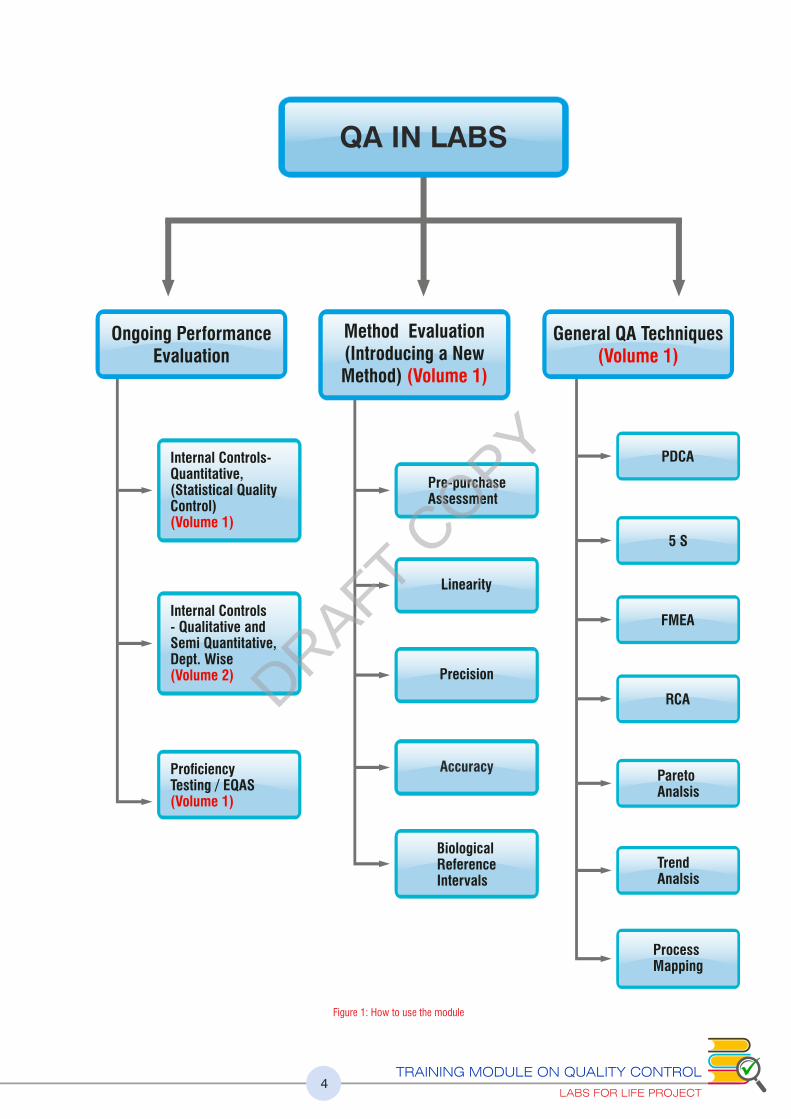
1.3 Objectives of the Module
The module is written keeping in mind the needs of Indian public health labs, to introduce the
concept of quality and to enable the implementation of a robust quality control system.
Assuring the quality of examinations is a requirement as per ISO 15189: 2012. Both internal
quality controls and external quality controls (Proficiency Testing) are discussed. Internal
controls are discussed with reference to daily monitoring using LJ charts as well as
evaluation of ongoing method performance using sigma metrics. Proficiency Testing (EQA)
will include the options of PT programs for different disciplines, interpretation of results and
remedial actions. In addition, Method Evaluation (ME) is included as it is also a requirement
of the ISO 15189:2012.
1.4 Target Audience
The target audience for this manual is the laboratory professionals, doctors and technicians
who do clinical laboratory testing.
1.5 Method
Regional trainings will be conducted for all institutions served by Labs for Life. Activity
sheets, handouts, PPTs than can be used for onward training are developed and distributed.
In addition, Labs for Life website has a QC toolkit for all the statistical activities described in
this manual. A digitalized version of this module will also be available soon on the Labs for
Life website.
1.6 How to Use the Module
This module is published in 2 volumes. In the first volume the statistical methods employed in
lab - Quality Controls; Internal and External; Method Evaluation and Continual Improvement
- are described. This as per the requirements of ISO 15189:2012, Clauses 5.6, 5.5 and 4.12.
In Volume 2 the Semi quantitative and qualitative control mechanisms used In Microbiology,
Hematology, Clinical Pathology, Histopathology and Cytology labs are explained.
DRAFT COPY
TRAINING MODULE ON QUALITY CONTROL
LABS FOR LIFE PROJECT4
QA IN LABS
Ongoing Performance Evaluation
General QA Techniques(Volume 1)
Method Evaluation(Introducing a New Method) (Volume 1)
Internal Controls-Quantitative,(Statistical Quality Control)(Volume 1)
Pre-purchaseAssessment
PDCA
5 S
FMEA
RCA
ParetoAnalsis
Trend Analsis
Process Mapping
Linearity
Precision
Accuracy
Internal Controls- Qualitative andSemi Quantitative,Dept. Wise(Volume 2)
ProficiencyTesting / EQAS(Volume 1)
BiologicalReferenceIntervals
Figure 1: How to use the module
DRAFT COPY

Chapter 1: Introduction This chapter describes the general overview of Quality Control in a lab, outlining the mechanism
for on-going performance evaluation using internal and external controls of different kinds. It also
outlines the need for Method Evaluation of any new test or equipment introduced to the lab.
Chapter 2: Internal Controls : Quantitative It outlines best practices in selecting control materials. The basic concepts in SQCs are then
explained in detail. How the characteristic feature - the Gaussian distribution of values - seen in
repeated examination of appropriately preserved biological material is made use of for
performance evaluation of methods and machines is explained. Every section is supported by
worksheets to reinforce the concept explained. The use of Internal QCs for plotting Levey
Jennings graph to assess the precision as well as shift in accuracy is detailed. The concept of more
advanced interpretations of IQC in terms of Total Error and Sigma metrics is also explained with
details of multi-rule selections in the case of poorly performing parameters. The concept of
Uncertainty of Measurement as a tool for reporting the confidence levels of a lab’s performance is
explained. Using a lot of QC as per new guidelines is described. Some specific control
mechanisms employed in certain equipments, such as radar graphs, Bull’s Algorithm are also
explained. The concept of harmonization of equipment as an indicator of comparability of
methods has been described.
Chapter 3: Proficiency Testing/ External Quality Assurance This chapter describes the mechanisms of testing the proficiency of your lab. It outlines the ISO
requirements therein and under this scope describes how several mechanisms of proficiency
testing can be interpreted. Details of scoring systems and judging acceptance as well as a list of
commonly used EQA Schemes in India is given.
Chapter 4: Method Evaluation
When a new test or equipment is introduced into a lab a mechanism for verifying this is required. A
mechanism may be incorporated into the purchase policy of the lab to assess the ‘fitness for use’
even before an equipment is purchased. These are explained in this chapter.
Chapter 5: General Concepts in Quality Assurance
ISO 15189 mandates that the lab monitor and assess performance and evolve mechanisms for
continual improvement. It also calls for risk assessment and risk management. This chapter
outlines a few of these mechanisms with examples.
VOLUME 1: STATISTICAL METHODS USED IN A LAB
Part 1: ON-GOING PERFORMANCE EVALUATION
Part 2: INTRODUCING A NEW METHOD OR EQUIPMENT
Part 3: CONTINUAL IMPROVEMENT
TRAINING MODULE ON QUALITY CONTROL
LABS FOR LIFE PROJECT5
DRAFT COPY
Chapter 6: Internal Control Semi Quantitative and
Qualitative Controls: Overview A general introduction to non-statistical methods of QCs are outlined in this chapter.
Chapter 7: QC in Microbiology and Serology, Quantitative, Semi
Quantitative and Qualitative All aspects of a microbiology lab including bacteriology, parasitology, and mycology are
explained. Antibiotic susceptibility testing mechanisms are described. Outlines of serology and
molecular diagnostics are also explained in terms of Quality Assurance.
Chapter 8: IQC (Qualitative) in Hematology and Clinical Pathology This chapter describes a few points to keep in mind, where making blood and bone marrow films
are concerned. Some general errors in doing ESR are pointed out. Control mechanisms including
pre-analytical and post analytical are enumerated for cavity uids, urine analysis and semen
analysis.
Chapter 9: Quality Assurance in Histopathology and Cytology The processes that happen in histopathology and cytology labs are several. Each step includes
chances of potential error. These should be understood and avoided as part of the quality
assurance process. To this end, each step in elaborated with suggestions of how to manage an
error free histopathology and cytology lab.
VOLUME 1: NON-STATISTICAL QUALITY CONTROLS
Part 4: On-going Evaluation of Method Performance:
Semi Quantitative and Qualitative Controls
TRAINING MODULE ON QUALITY CONTROL
LABS FOR LIFE PROJECT6
DRAFT COPY

VOLUME 1
7
ONGOING EVALUATION
OF METHOD
PERFORMANCE
PART 1
ISO 15189:2012 5.6
ASSURING THE QUALITY OF EXAMINATIONS
DRAFT COPY

TRAINING MODULE ON QUALITY CONTROL
LABS FOR LIFE PROJECT8
Learning Objectives
At the end of this chapters the learners will be able to answer the following questions:
How to select, reconstitute, store and use the quality control materials
The details of quality control material
Evolution of Quality Control techniques and monitoring mechanism
through statistical process like LJ, Total Error and sigma metrics
How to handle a new lot of quality control
How to set quality requirements for a lab
How to plan a QC program in a lab
Concepts of Uncertainty of Measurement
CHAPTER 2: INTERNAL CONTROLS:
QUANTITATIVE (STATISTICAL QUALITY CONTROLS)
“Quantitative tests measure the quantity of a substance in a sample, yielding a numeric result. For
example, the quantitative test for glucose can give a result of 110 mg/dL. Since quantitative tests have
numeric values, statistical tests can be applied to the results of quality control material to differentiate
between test runs that are “in control” and “out of control”. This is done by calculating acceptable
limits for control material.
As a part of the quality management system, the laboratory must establish a quality control program
for all quantitative tests. Evaluating each test run in this way allows the laboratory to determine if
patient results are accurate and reliable.
2.1. Internal Controls: Overview
2.1 (a) Characteristics of Control Materials
It is critical to select the appropriate control materials. Some important characteristics to
consider when making the selection.
• Controls must be appropriate for the targeted diagnostic test–the substance being
measured in the test must be present in the control in a measurable form.
• The amount of the analyte present in the controls should be close to the medical
decision points of the test; this means that controls should check both low values
and high values.
• Controls should have the same matrix as patient samples; this usually means that the
controls are serum-based, but they may also be based on plasma, urine, or other materials.
• Because it is more efficient to have controls that last for some months, it is best to
obtain control materials in large quantity.
• The shelf life and open vial stability of the control should be good, with minimal vial to
vial variability and should be stable for long periods of time.
DRAFT COPY
TRAINING MODULE ON QUALITY CONTROL
LABS FOR LIFE PROJECT9
• Should be simple to use.
• Liquid controls are more convenient than lyophilized controls because they do not
have to be reconstituted minimizing pipetting error.
• The assayed control providers should provide a robust Inter Laboratory Comparison
Program.
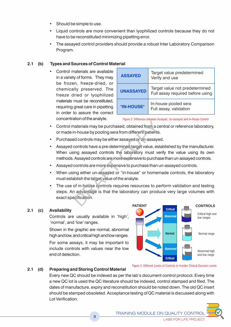
2.1 (b) Types and Sources of Control Material
• Control materials are available
in a variety of forms. They may
be frozen, freeze-dried, or
chemically preserved. The
freeze dried or lyophilized
materials must be reconstituted,
requiring great care in pipetting
in order to assure the correct
concentration of the analyte.
• Control materials may be purchased, obtained from a central or reference laboratory,
or made in-house by pooling sera from different patients.
• Purchased controls may be either assayed or un-assayed.
• Assayed controls have a pre-determined target value, established by the manufacturer.
When using assayed controls the laboratory must verify the value using its own
methods. Assayed controls are more expensive to purchase than un-assayed controls.
• Assayed controls are more expensive to purchase than un-assayed controls.
• When using either un-assayed or “in-house” or homemade controls, the laboratory
must establish the target value of the analyte.
• The use of in-house controls requires resources to perform validation and testing
steps. An advantage is that the laboratory can produce very large volumes with
exact specification.
2.1 (c) Availability
Controls are usually available in ‘high’,
‘normal’, and ‘low’ ranges.
Shown in the graphic are normal, abnormal
high and low, and critical high and low ranges.
For some assays, it may be important to
include controls with values near the low
end of detection.
2.1 (d) Preparing and Storing Control Material
Every new QC should be indexed as per the lab’s document control protocol. Every time
a new QC lot is used the QC literature should be indexed, control stamped and filed. The
dates of manufacture, expiry and reconstitution should be noted down. The old QC insert
should be stamped obsoleted. Acceptance testing of QC material is discussed along with
Lot Verification.
ASSAYEDTarget value predetermined Verify and use
UNASSAYEDTarget value not predetermined Full assay required before using
"IN-HOUSE"In-house pooled seraFull assay, validation
Figure 2: Difference between Assayed, Un-assayed and In-House Control
PATIENTCritical
Abnormal
Normal
Abnormal
Critical
CONTROLS
Critical high andlow ranges
Normal range
Abnormal highand low range
Figure 3: Different Levels of Controls to monitor Clinical Decision Levels
DRAFT COPY

TRAINING MODULE ON QUALITY CONTROL
LABS FOR LIFE PROJECT10
2.1 (e) Reconstitution Procedure
When preparing and storing quality control materials it is important to carefully adhere to
the manufacturer’s instructions for reconstituting and for storage. Reconstitution of QCs,
whether internal or external, should be done with utmost caution. Use a calibrated pipette
to deliver the exact amount of required diluent to lyophilized controls that are
reconstituted. It would be ideal to use a separate pipette for reconstitution. Carefully
including every particle of the lyophilized material stuck to the bottom of the cap is vital.
Reconstitution errors can masquerade as system errors and lead to unnecessary
corrective actions. Replace the stopper and allow to stand for the time specified, swirling
occasionally. Before sampling, gently swirl the vial several times to ensure homogeneity.
2.1 (f) Storage and Stability
The instructions of the manufacturer should be followed for storage of both unopened
and opened vials. For in-house controls, protocols of storage must be done using
validated procedures. Divide into aliquots of appropriate volumes and store at -10 °C to -
20°C or as specified by the manufacturer. Care should be taken that the aliquots made will
not be used beyond the date of expiry. The frozen samples should be thawed at room
temperature before being used for assays. Do not thaw and re-freeze control material.
Monitor and maintain freezer temperatures to avoid degradation of the analyte in any
frozen control material.
In the case of liquid controls, understand the storage requirements, the need for aliquoting.
In the case of hematology controls, there the guidelines on the maximum number of cap
opening or piercing should be understood and followed.
If in-house control material is used, freeze aliquots and place in the freezer so that a small
amount can be thawed and used daily. An example of a QC insert is given below:
REF 692 Level 2 25 x 10 mL
690X Bilevel MiniPak 2 x 10 mL IVD
Figure 4: An Example of QC insert
DRAFT COPY

TRAINING MODULE ON QUALITY CONTROL
LABS FOR LIFE PROJECT11
2.1. (g) Purchasing Quality Controls
We expect QC materials to provide information about what is occurring with the
measurement procedure. In other words, we expect the performance of the QC materials
to mirror the same effects as what is occurring to our patient samples.
To do this, QC materials should:
1) Mimic the matrix and viscosity of the patient samples being tested
• Matrix—the base from which control materials are prepared in addition to the
preservatives added for stability
• Matrix effect – the inuence of the control material’s matrix, other than the
concentration of the analyte, on the measurement procedure to produce differing
results when compared to other methods while still producing consistent results
on patient samples
2) Be both physically and chemically sensitive to changes in the measurement procedure
as patient samples
3) Contain concentrations of analytes at or near medical decision points
4) Be available in one lot number that is stable for an extended period of time
5) Be available at different concentration levels to assess the measuring range of
the method
6) Remain stable before and after opening a vial as indicated by the manufacturer
7) Produce minimal vial-to-vial variability
In addition to the above stated qualities, other considerations that should be kept in mind are:
1) Use of lyophilized (freeze-dried) controls
• Usually less costly per box than liquid.
• Require a special diluent or deionized Type I water.
• Require availability of clean Class ‘A’ Volumetric pipets and pipetting bulbs.
• Require staff that is capable of
• Accurately pipetting manually Strictly adhering to reconstitution and mixing
instructions provided by the manufacturer
• May experience more vial-to-vial variability (increase imprecision) especially if
improper handling and reconstitution occurs
• Frequently has a shorter opened vial expiry interval
• May result in discarding unused portion (hidden cost consideration)
2) Use of liquid controls
• Usually more costly per box than lyophilized
• Eliminates many of the handling and reconstitution errors
• Inuence of matrix effect may be greater with the method you use
• Frequently has a longer opened vial expiry interval
• May discard less or none of the product if consumed within opened expiry date
DRAFT COPY
TRAINING MODULE ON QUALITY CONTROL
LABS FOR LIFE PROJECT12
3) Frequency of lot number changes
• Performing parallel testing takes time and money (costs of performing testing on
QC materials)
• With each QC material lot number change, lose access to summary or
cumulative data
• Recommend to purchase a year supply of the same lot number, when possible
but taking into consideration the following:
Desired expiration date should be specified at time of purchase
Storage issues
Difficulties encountered with setting up a standing order with the vendor
4) Vendor considerations
• Availability of an inter-laboratory comparison program
• Provide troubleshooting support
• Ability to accommodate standing orders
• Ability to sequester specified lot number and automatically ship and bill as
outlined in the purchase agreement
2.1. (h) Classification of Control Material
Dependent control material is a quality control material manufactured under the
same quality system as the instrument, kit or method it is intended to monitor and
whose performance depends on design inputs from the instrument, kit or method
manufacturer.
Dependent controls are typically provided by the instrument manufacturer. This type
of control material also includes what is referred to as “in kit” controls; those control
materials provided as a part of a discrete test kit. Dependent control materials are
often manufactured from the same lot of raw material, using the same manufacturing
process, and made in the same facility used to manufacture the instrument, kit or
method calibrators. At some point, the manufacturing process for controls and
calibrators splits.
Independent (Third Party) Control Material is manufactured outside the quality
system used to manufacture the instrument, kit or method it is intended to monitor and
whose performance is independent of any design inputs from the instrument, kit or
method manufacturer.
Quality control material (assayed or un-assayed) is a medical device intended for use in a
test system to estimate test precision and detect systematic analytical deviations that may
arise from reagent or analytical instrument variation
Semi-dependent control material is manufactured outside the quality system used to
manufacture the instrument, kit or method it is intended to monitor but is manufactured on
behalf of and with input from the instrument, kit or method manufacturer.
DRAFT COPY
TRAINING MODULE ON QUALITY CONTROL
LABS FOR LIFE PROJECT13
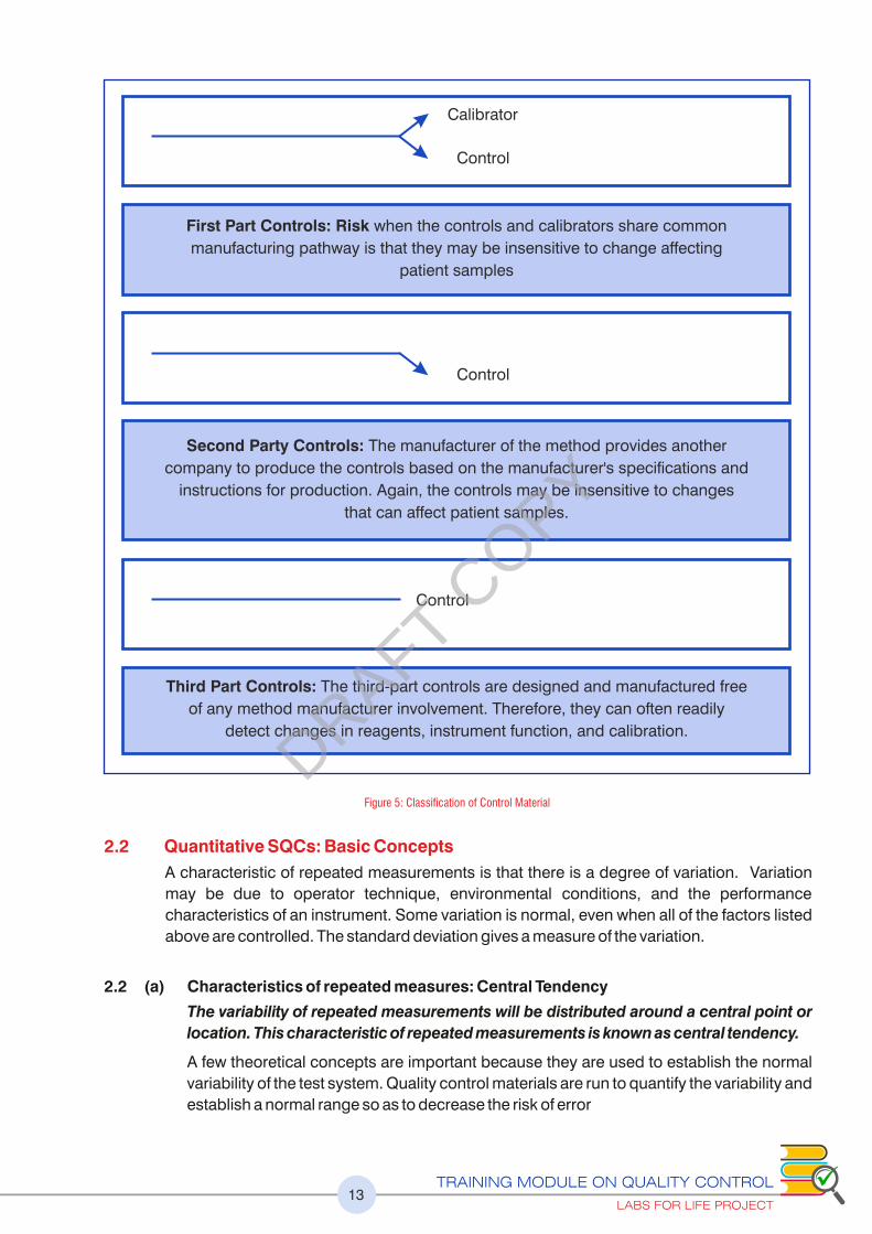
Calibrator
Control
First Part Controls: Risk when the controls and calibrators share common
manufacturing pathway is that they may be insensitive to change affecting
patient samples
Control
Second Party Controls: The manufacturer of the method provides another
company to produce the controls based on the manufacturer's specifications and
instructions for production. Again, the controls may be insensitive to changes
that can affect patient samples.
Control
Third Part Controls: The third-part controls are designed and manufactured free
of any method manufacturer involvement. Therefore, they can often readily
detect changes in reagents, instrument function, and calibration.
Figure 5: Classification of Control Material
2.2 Quantitative SQCs: Basic Concepts
A characteristic of repeated measurements is that there is a degree of variation. Variation
may be due to operator technique, environmental conditions, and the performance
characteristics of an instrument. Some variation is normal, even when all of the factors listed
above are controlled. The standard deviation gives a measure of the variation.
2.2 (a) Characteristics of repeated measures: Central Tendency
The variability of repeated measurements will be distributed around a central point or
location. This characteristic of repeated measurements is known as central tendency.
A few theoretical concepts are important because they are used to establish the normal
variability of the test system. Quality control materials are run to quantify the variability and
establish a normal range so as to decrease the risk of error
DRAFT COPY

TRAINING MODULE ON QUALITY CONTROL
LABS FOR LIFE PROJECT14
We use statistical terms to describe something about a set of data points. With a
specific data set, it is often important to know the values around which the observations
tend to cluster. Three measures of the "center" of the data are the mean, the median,
and the mode.
Mean ( x ) the arithmetic average of results. The mean is the most commonly used
measure of central tendency used in laboratory QC)
The mean, also called the arithmetic mean or the average, is the sum of all the data points
divided by the number of points. The average is the most common way of calculating
central tendency.
Example: For the data set containing 7 numbers {2, 5, 9, 3, 5, 7, and 4}, the mean is
calculated as:
2+5+9+3+5+7+4 = 35/7 = 5 is the mean
Some of its characteristics are:
• easy to calculate
• only one exists for any data set
• affected by all observations, and strongly affected by outliers
Median (the central point of the values when they are arranged in numerical sequence.)
The median of a data set is the value of the middle point, when they are arranged in order.
Using the previous data set and arranging from lowest to highest {2, 3, 4, 5, 5, 7, 9}, we
can determine the median by crossing off the lowest and highest values, then the next
lowest and next highest value. Continue crossing off values from both ends until only one
value, the middle value, remains {2, 3, 4, 5, 5, 7, and 9}. For this data set, the median is 5.
If there is an even number of points, average the two middle values.
Example: For the following data set containing 6 numbers, {2, 3, 4, 5, 7, 9}, we can
determine the median as follows: 2, 3, 4, 5, 7, 9. for this data set, two numbers, 4 and 5, lie
at the center. To determine the median for this data set, we would take the average of 4
and 5 as follows:
4+5 = 9/2 = 4.5. The median for this data set is 4.5.
Some characteristics of the median are:
• always exists for a set of data
• unique
• not strongly affected by extreme values
• corresponds to the 50th percentile
Mode (the number that occurs most frequently).
The mode is the value that occurs most frequently in a data set. There can be more than
one mode, if there are two or more values that are tied for occurring most frequently. In
cases where two numbers occur most frequently, the distribution of data would then be
classified as bimodal (having two modes).
For the data set, {2, 5, 9, 3, 5, 7, 4}, all numbers occur only once except the number 5; it
occurs twice, or more frequently than the other numbers. Therefore, the mode for this
data set is 5.
DRAFT COPY

TRAINING MODULE ON QUALITY CONTROL
LABS FOR LIFE PROJECT15
The properties of the mode are:
• requires no calculation
• not necessarily unique
• very insensitive to extreme values
• may not be close to the center of the distribution
Please refer to exercise no.1
2.2 (b) Normal Distribution: Gaussian is the Key
In probability theory, the normal (or Gaussian) distribution is a very common continuous
probability distribution. Normal distributions are important in statistics and are often used
in the natural and social sciences to represent real-valued random variables whose
distributions are not known. The normal distributions are a very important class of
statistical distributions. All normal distributions are symmetric and have bell-shaped
density curves with a single peak. To speak specifically of any normal distribution, two
quantities have to be specified: the mean, where the peak of the density occurs, and the
standard deviation, which indicates the spread or girth of the bell curve.
Many things closely follow a Normal Distribution: heights of people, data points in
measurements and blood pressure.
See the distributions below:
Please refer to exercise no.2
2.2 (c) Some Statistical Notations
Statistical notations are symbols used in mathematical formulas to calculate statistical
measures. For this module, the symbols that are important to know are:
�:��the sum of
N: number of data points (results or observations)
x : the symbol for the mean.
The square root of the data. :
� :�Standard Deviation
Figure 6: Different Kinds of Distribution
DRAFT COPY
TRAINING MODULE ON QUALITY CONTROL
LABS FOR LIFE PROJECT16
2.2 (d) Standard Deviation
Standard Deviation (SD) is a measurement of variation in a set of results. It is the statistic
that quantifies how close numerical values (i.e., QC values) are in relation to each other.
The term precision is often used interchangeably with standard deviation. Another term,
imprecision, is used to express how far apart numerical values are from each other.
Standard deviation is calculated for control products from the same data used to
calculate the mean. It provides the laboratory an estimate of test consistency at specific
concentrations. The repeatability of a test may be consistent (low standard deviation, low
imprecision) or inconsistent (high standard deviation, high imprecision). Inconsistent
repeatability may be due to the chemistry involved or to a malfunction. If it is a
malfunction, the laboratory must correct the problem. It is very useful to the laboratory in
analyzing quality control results.
The formula for calculating standard deviation is:
The number of independent data points (values) in a data set are represented by “n”
Please refer to exercise no.3
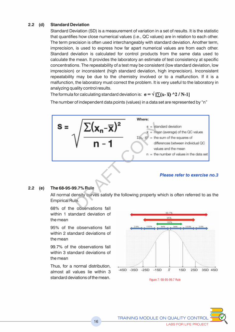
2.2 (e) The 68-95-99.7% Rule
All normal density curves satisfy the following property which is often referred to as the
Empirical Rule.
68% of the observations fall
within 1 standard deviation of
the mean
95% of the observations fall
within 2 standard deviations of
the mean
99.7% of the observations fall
within 3 standard deviations of
the mean
Thus, for a normal distribution,
almost all values lie within 3
standard deviations of the mean.Figure 7: 68-95-99.7 Rule
DRAFT COPY

TRAINING MODULE ON QUALITY CONTROL
LABS FOR LIFE PROJECT17
2.2 (f) Establishing the Value Range for the Control Material
Stable analytical systems will produce the same Gaussian distribution of data when a
stable material is run on it, over a period of time. When a system undergoes a change, an
unexpected data point will be produced.
One of the most important goals of a quality control program is to differentiate between
normal variation and errors.
Collecting data
Once the appropriate control materials are purchased or prepared, the next step is to
determine the range of acceptable values for the control material. This will be used to let
the laboratory know if the test run is “in control” or if the control values are not reading
properly – “out of control”.
This is done by assaying the control material repeatedly over time. At least 20 data points
must be collected over a 20 to 30 day period. When collecting this data, be sure to include
any procedural variation that occurs in the daily runs; for example, if different testing
personnel normally do the analysis, all of them should collect part of the data.
Once the data is collected, the laboratory will need to calculate the mean and standard
deviation of the results. Labs For Life QC Tool : Parallel testing of QC
The purpose of obtaining 20 data points by running the quality control sample is to
quantify normal variation, and establish ranges for quality control samples. Use the
results of these measurements to establish QC ranges for testing.
If one or two data points appear to be too high or low for the set of data, they should not be
included when calculating QC ranges. They are called “outliers”.
If there are more than 2 outliers in the 20 data
points, there is a problem with the data and it
should not be used. Identify and resolve the
problem and repeat the data collection.
The measurements are taken when plotted on a
graph, it must form a bell-shaped curve as the
results vary around the mean as a normal
distribution (Gaussian distribution).
The distribution can be seen if data points are
plotted on the x-axis and the frequency with
which they occur on the y-axis.
Calculating the Mean, SD, Range
Also, needing calculation are the Mean and the Standard Deviation as explained above.
Once the mean and the Standard Deviation are understood, the range of acceptability
can be assigned and a chart can be developed used to plot the daily control values.
• To calculate 1 SD, add and subtract the value from the mean.
• To calculate 2 SDs, multiply the SD by 2 then add and subtract each result
from the mean.
• To calculate 3 SDs, multiply the SD by 3, then add and subtract each result
from the mean.
Figure 8: Gaussian distribution plotted alongside time frequency
DRAFT COPY

TRAINING MODULE ON QUALITY CONTROL
LABS FOR LIFE PROJECT18
For a mean of 190.5 and an SD of 2, therefore:
• ±1 SD is 188.5 - 192.5
• ±2 SD is 186.5 - 194.5, and
• ± 3 SD is 184.5 - 196.5.
The range of acceptability is ± 3 SD
Once these ranges are established, they can be used to evaluate a test run. For example,
if you examine a control with your patients’ samples and get a value of 193.5, you know
there is a 95.5% chance that it is within 2 SD of the mean.
When an analytical process is within control, approximately 68% of all QC values fall
within ±1 standard deviation (1s). Likewise 95.5% of all QC values fall within ±2 standard
deviations (2s) of the mean. About 4.5% of all data will be outside the ±2s limits when the
analytical process is in control. Approximately 99.7% of all QC values are found to be
within ±3 standard deviations (3s) of the mean. As only 0.3%, or 3 out of 1000 points, will
fall outside the ±3s limits, any value outside of ±3s is considered to be associated with a
significant error condition and patient results should not be reported.
2.2 (g) Graphically Representing Control Ranges: Levey-Jennings Charts
The laboratory needs to document that quality control materials are assayed and that the
quality control results have been inspected to assure the quality of the analytical run. This
documentation is accomplished by maintaining a QC Log and using the Levey-Jennings
chart on a regular basis. The QC Log can be maintained on a computer or on paper. The log
should identify the name of the test, the instrument, units, the date the test is performed, the
initials of the person performing the test, and the results for each level of control assayed.
The Levey-Jennings charts represent the range graphically for the purpose of daily
monitoring.
A Levy-Jennings chart can then be drawn, showing the mean value as well as plus/minus
1, 2, and 3 standard deviations (SD). The mean is shown by drawing a line horizontally in
the middle of the graph and the SD are marked off at appropriate intervals and lines drawn
horizontally on the graph as shown below.
Figure 9: Blank Levy-Jennings chart with defined mean and SD
DRAFT COPY

TRAINING MODULE ON QUALITY CONTROL
LABS FOR LIFE PROJECT19
In order to use the Levey-Jennings chart to record and monitor daily control values,
label the x-axis with days, runs, or other interval used to run QC. Label the chart with the
name of the test and the lot number of the control being used. On a daily basis, enter
values on the chart.
An LJ is basically a Gaussian on its side, separated by time as a frequency. If you look
at the figures above and below, this can be understood.
Please refer to exercise no.4
Figure 10: A Gaussian on its side with a frequency, is a LJ Chart
Figure 11: 68-95-99.7 Rule on LJ Chart
DRAFT COPY

TRAINING MODULE ON QUALITY CONTROL
LABS FOR LIFE PROJECT20
2.3 Interpreting Quality Control Data: LJ Charts
2.3 (a) Training your Eyes to Identify Errors and Changes in Pattern
From the above discussion it is evident that the patterns can be easily discerned by eyes
once it is graphically represented. This discernment should be both in terms of daily
assessments and periodic assessments. A set of rules have been defined that can be
used singularly (single rules) or in combination (multi-rules), depending on the
performance of the parameter and as protocoled by the lab.
In the following sections, we will examine the rules, the errors, concepts of accuracy
and precision, how to apply the rules to detect errors, how to define the optimum QC
protocol for each analyte.
2.3 (b) The Westgard Rules:
In 1981, Dr. James Westgard of the University of Wisconsin published an article on
laboratory quality control that set the basis for evaluating analytical run quality for medical
laboratories. The elements of the Westgard system are based on principles of statistical
process control used in industry since the 1950s.There are several rules in the Westgard
scheme. These rules are used individually or in combination to evaluate the quality of
analytical runs.
Westgard devised a shorthand notation for expressing quality control rules. Most of the
quality control rules can be expressed as NL where N represents the number of control
observations to be evaluated and L represents the statistical limit for evaluating the
control observations. Thus 1:3s or 13s represents a control rule that is violated when one
control observation exceeds the ±3s control limits.
1. 1:3s or 1 s refers to a control rule that is commonly used with a Levey-Jennings chart 3
when the control limits are set as the mean plus 3s and the mean minus 3s. A run is
rejected when a single control measurement exceeds the mean plus 3s or the mean
minus 3s control limit. This rule identifies unacceptable random error or possibly the
beginning of a large systematic error. Any QC result outside ±3s violates this rule.
st nd1 and 2 GENERATION QCs: LJs, RULES, MULTI-RULES AND RULE VIOLATIONS
Figure 12: 1:3s or 1: S denotes a Random Error or a beginning of a Systematic Error3
DRAFT COPY
TRAINING MODULE ON QUALITY CONTROL
LABS FOR LIFE PROJECT21
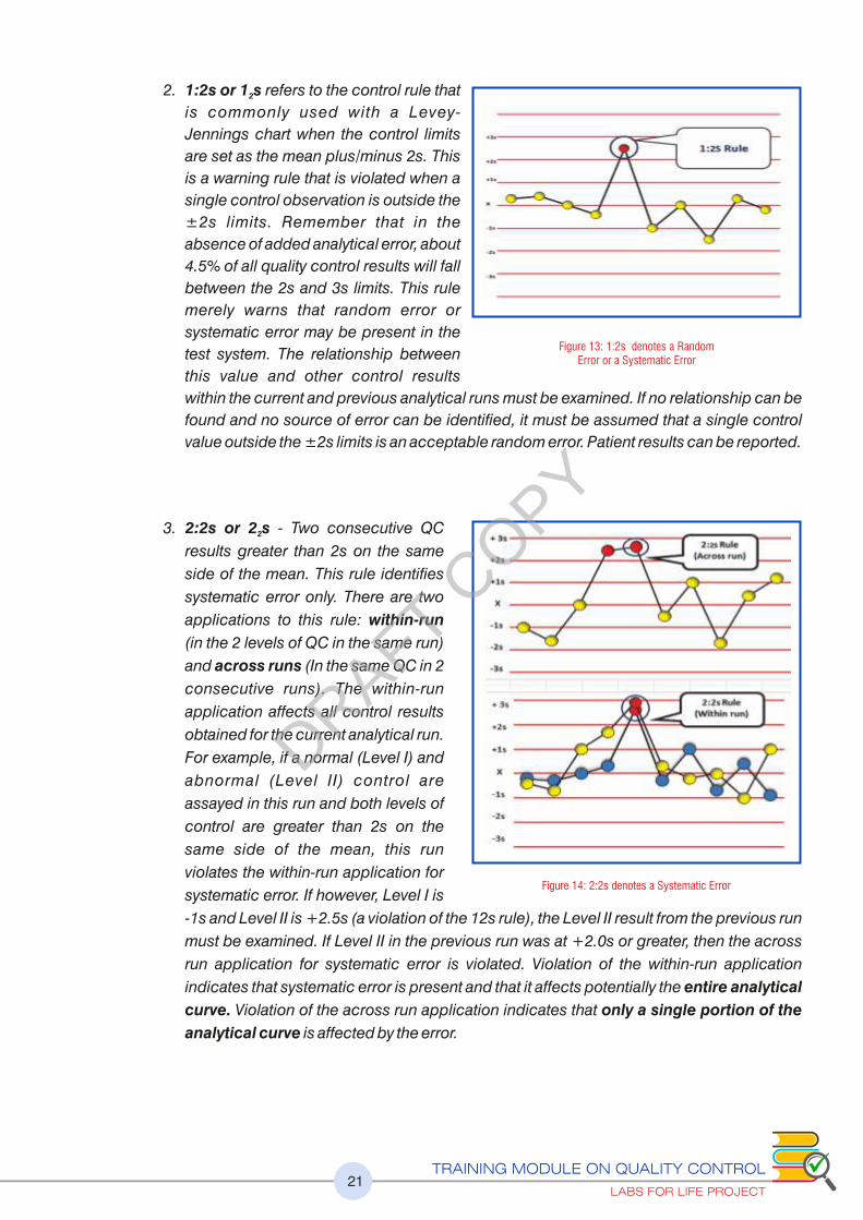
2. 1:2s or 1 s refers to the control rule that 2
is commonly used with a Levey-
Jennings chart when the control limits
are set as the mean plus/minus 2s. This
is a warning rule that is violated when a
single control observation is outside the
±2s limits. Remember that in the
absence of added analytical error, about
4.5% of all quality control results will fall
between the 2s and 3s limits. This rule
merely warns that random error or
systematic error may be present in the
test system. The relationship between
this value and other control results
within the current and previous analytical runs must be examined. If no relationship can be
found and no source of error can be identified, it must be assumed that a single control
value outside the ±2s limits is an acceptable random error. Patient results can be reported.
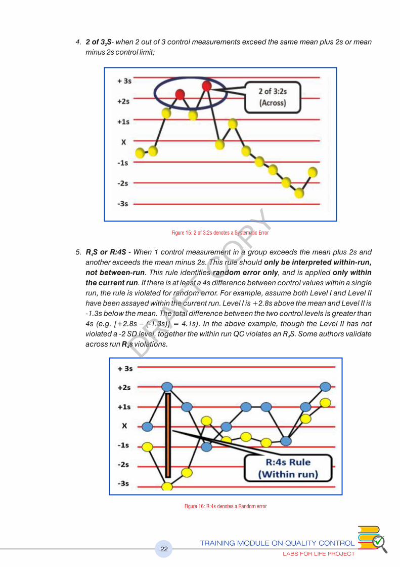
3. 2:2s or 2 s - Two consecutive QC 2
results greater than 2s on the same
side of the mean. This rule identifies
systematic error only. There are two
applications to this rule: within-run
(in the 2 levels of QC in the same run)
and across runs (In the same QC in 2
consecutive runs). The within-run
application affects all control results
obtained for the current analytical run.
For example, if a normal (Level I) and
abnormal (Level II) control are
assayed in this run and both levels of
control are greater than 2s on the
same side of the mean, this run
violates the within-run application for
systematic error. If however, Level I is
-1s and Level II is +2.5s (a violation of the 12s rule), the Level II result from the previous run
must be examined. If Level II in the previous run was at +2.0s or greater, then the across
run application for systematic error is violated. Violation of the within-run application
indicates that systematic error is present and that it affects potentially the entire analytical
curve. Violation of the across run application indicates that only a single portion of the
analytical curve is affected by the error.
Figure 13: 1:2s denotes a Random Error or a Systematic Error
Figure 14: 2:2s denotes a Systematic Error
DRAFT COPY
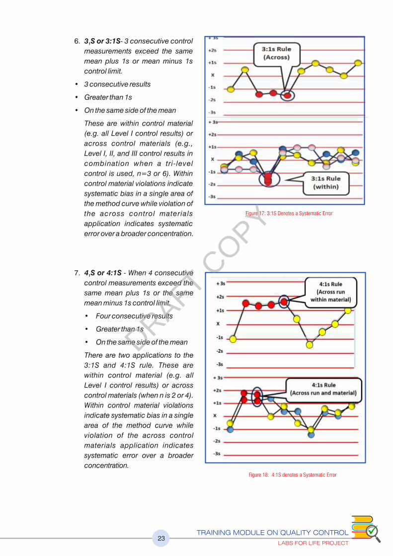
4. 2 of 3 S- when 2 out of 3 control measurements exceed the same mean plus 2s or mean 2
minus 2s control limit;
5. R S or R:4S - When 1 control measurement in a group exceeds the mean plus 2s and 4
another exceeds the mean minus 2s. This rule should only be interpreted within-run,
not between-run. This rule identifies random error only, and is applied only within
the current run. If there is at least a 4s difference between control values within a single
run, the rule is violated for random error. For example, assume both Level I and Level II
have been assayed within the current run. Level I is +2.8s above the mean and Level II is
-1.3s below the mean. The total difference between the two control levels is greater than
4s (e.g. [+2.8s – (-1.3s)] = 4.1s). In the above example, though the Level II has not
violated a -2 SD level, together the within run QC violates an R S. Some authors validate 4
across run R s violations. 4
TRAINING MODULE ON QUALITY CONTROL
LABS FOR LIFE PROJECT22
Figure 15: 2 of 3:2s denotes a Systematic Error
Figure 16: R:4s denotes a Random error
DRAFT COPY
TRAINING MODULE ON QUALITY CONTROL
LABS FOR LIFE PROJECT23
6. 3 S or 3:1S- 3 consecutive control 1
measurements exceed the same
mean plus 1s or mean minus 1s
control limit.
• 3 consecutive results
• Greater than 1s
• On the same side of the mean
These are within control material
(e.g. all Level I control results) or
across control materials (e.g.,
Level I, II, and III control results in
combination when a tri-level
control is used, n=3 or 6). Within
control material violations indicate
systematic bias in a single area of
the method curve while violation of
the across control materials
application indicates systematic
error over a broader concentration.
7. 4 S or 4:1S - When 4 consecutive 1
control measurements exceed the
same mean plus 1s or the same
mean minus 1s control limit.
• Four consecutive results
• Greater than 1s
• On the same side of the mean
There are two applications to the
3:1S and 4:1S rule. These are
within control material (e.g. all
Level I control results) or across
control materials (when n is 2 or 4).
Within control material violations
indicate systematic bias in a single
area of the method curve while
violation of the across control
materials application indicates
systematic error over a broader
concentration.
Figure 17: 3:1S Denotes a Systematic Error
Figure 18: 4:1S denotes a Systematic Error
DRAFT COPY

TRAINING MODULE ON QUALITY CONTROL
LABS FOR LIFE PROJECT24
8. 6x, 8x,9x, 10x, 12x
These rules are violated when
there are: 6 or 8, or 9, or 10, or 12
control results on the same side of
the mean regardless of the
specific standard deviation in
which they are located.
Each of these rules also has two
appl icat ions: wi thin control
material (e.g., all Level I control
results) or across control materials
(e.g. Level I, II, and III control results
in combination). Within control
mater ia l v io la t ions indicate
systematic bias in a single area of the
method curve while violation of the
across control materials application
indicates systematic bias.
9. 7 - When seven control measurements trend in the same direction, crossing the mean, T
i.e., get progressively higher or progressively lower. Applicable across run
Please refer to exercise no.5
Figure 19: 10x rule denotes Systematic Errors
6x, 8x,9x, 10x, 12x denotes Systematic Errors
Figure 20:7T denotes a Systematic Error
DRAFT COPY

TRAINING MODULE ON QUALITY CONTROL
LABS FOR LIFE PROJECT25
2.3 (c) Using Only One Level Control
If it is possible to use only one control, choose one with a value that lies within the normal
range of the analyte being tested. When evaluating results, accept all runs where the
control lies within + 2 SD. Using this system, the correct value will be rejected 4.5% of the
time (False Rejects).
2.3 (d) Using the Rules: Single Rule and Multi
Rules
Please refer section 2.8 QC Planning for
the details of using QC rules in Lab.
2.3 (e) Concepts of Accuracy, Precision and
Total Error
If a measurement is repeated many times,
the result should be a mean that is very
close to the true mean.
1) Accuracy is the closeness of a
measurement to its target/ true value (explained later). When the mean changes
from the true mean, there is measuring system is said to have a systematic error or
bias Systematic error is evidenced by a change in the mean of the control values.
2) The change in the mean may be gradual and demonstrated as a trend in control
values or it may be abrupt and demonstrated as a shift in control values. Bias is the
difference between true or target value and the obtained value.
Target Value may be obtained from
1) Inter-laboratory comparison programs of the QC manufacturer. Good QC
providers give monthly as well as cumulative means. The cumulative means are
robust value and will give very good anchoring of the true value
2) Manufacturer assigned mean
3) Long term lab mean provided the QC lot has been running for a considerable
duration.
Figure 21: Concept of bias in performance
Figure 22: Differences between Random & Systematic Errors
DRAFT COPY

TRAINING MODULE ON QUALITY CONTROL
LABS FOR LIFE PROJECT26
Bias values have direction, it may be Positive or Negative, depending on if the obtained
value is higher or lower than the target. It is thus imperative that the absolute value be
obtained from the actual bias. Acceptable Bias values are available in BV Charts
(Annexure no 2:A )
Bias thus has a value which can be used to eliminate or minimize the offset e.g. by
recalibration or by adjusting raw results with a correction factor.
3) Precision is the amount of variation in the measurements, a deviation away from an
expected result and is computed as Random Error. The acceptable (or expected)
variations are defined and quantified by standard deviation. There are unacceptable
(unexpected) variations when any data point falls outside the expected population of
data. The less variation a set of measurements has, the more precise it is. The variation
thus is measured in Standard Deviations. In more precise measurements, the width of the
Gaussian curve is smaller because the measurements are all closer to the mean. The rule
violations will happen in the tails of the Gaussian or upper and lower ends of LJ typically
as R S or 1 S violations.4 3
4) Total Error is the combined value of both accuracy and precision (Discussed later)
The reliability of a method is thus
judged in terms of accuracy and
precision which contributes to
the Total Error. A simple way to
portray precision and accuracy
is to think of a target with a
bull’s eye.
The bull’s eye represents the
accepted reference value which is
the true, unbiased value. If a set of
data is clustered around the bull’s
eye, it is accurate. The closer
together the hits are, the more precise they are. If most of the hits are in the bull’s eye, as in
the figure on the left, they are both precise and accurate.
The values in the middle figure are precise but not accurate because they are clustered
together but not at the bull’s eye. The figure on the right shows a set of hits that are
imprecise. Measurements can be precise but not accurate if the values are close together
but do not hit the bull’s eye. These values are said to be biased. The middle figure
demonstrates a set of precise but biased measurements.
The purpose of quality control is to monitor the accuracy and precision of laboratory
assays before releasing patient results.
TE= SE + RE, where SE is the Systematic Error (Bias) calculated by
subtracting the Obtained Lab Mean from the True (Target) Mean and
RE is 1.65 (Z Factor)* SD (or CV)
Figure 23: Difference between Accuracy & Precision
DRAFT COPY

TRAINING MODULE ON QUALITY CONTROL
LABS FOR LIFE PROJECT27
2.3 (f) What Errors can be Detected on the LJ?
Using the LJ graph the following points can be discerned. Look at the examples below.
1. Errors in precision are easily detected. See increasing imprecision towards the
second half of the LJ contributing to increased Random Error (Figure 24)
2. A change in accuracy can be observed as an emerging population of data points with
a new mean developing indicating a Systematic change (Figure 25)
3. If the Target or True value (explained later) is available, it can be discerned if you are
changing for a better or a worse accuracy (explained later)
Figure 24: Imprecision
Figure 25: Shifting Accuracy
Figure 26: Recap Increasing Imprecision and Shifting Accuracy (a) (b)
(a) Imprecision: Errors in the tails. Widening Gaussian(b) Change in accuracy: Emerging populations.
Multiple, overlapping Gaussians
DRAFT COPY

Figure 27: Recap (Real time) Increasing Imprecision and Shifting Accuracy (a) (b)
Figure 28: Recap on shifting accuracy and increasing imprecision on a Gaussian: Shifting accuracy (a to c). In figure (a)
the two populations are overlapping and is difficult to distinguish an emerging population. In figure (b & c) the shift
becomes more pronounced and can be easily understood. In figure (d) increasing imprecision gives rise to populations
outside the original Gaussian (Widening Gaussian in pink).
TRAINING MODULE ON QUALITY CONTROL
LABS FOR LIFE PROJECT28
DRAFT COPY
TRAINING MODULE ON QUALITY CONTROL
LABS FOR LIFE PROJECT29
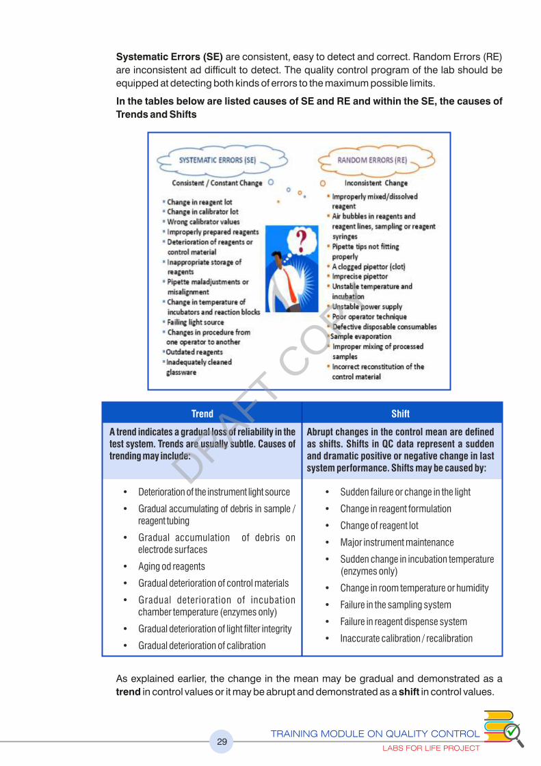
Systematic Errors (SE) are consistent, easy to detect and correct. Random Errors (RE)
are inconsistent ad difficult to detect. The quality control program of the lab should be
equipped at detecting both kinds of errors to the maximum possible limits.
In the tables below are listed causes of SE and RE and within the SE, the causes of
Trends and Shifts
As explained earlier, the change in the mean may be gradual and demonstrated as a
trend in control values or it may be abrupt and demonstrated as a shift in control values.
Trend
A trend indicates a gradual loss of reliability in the test system. Trends are usually subtle. Causes of trending may include:
• Deterioration of the instrument light source
• Gradual accumulating of debris in sample / reagent tubing
• Gradual accumulation of debris on electrode surfaces
• Aging od reagents
• Gradual deterioration of control materials
• Gradual deterioration of incubation chamber temperature (enzymes only)
• Gradual deterioration of light filter integrity
• Gradual deterioration of calibration
Shift
Abrupt changes in the control mean are defined as shifts. Shifts in QC data represent a sudden and dramatic positive or negative change in last system performance. Shifts may be caused by:
• Sudden failure or change in the light
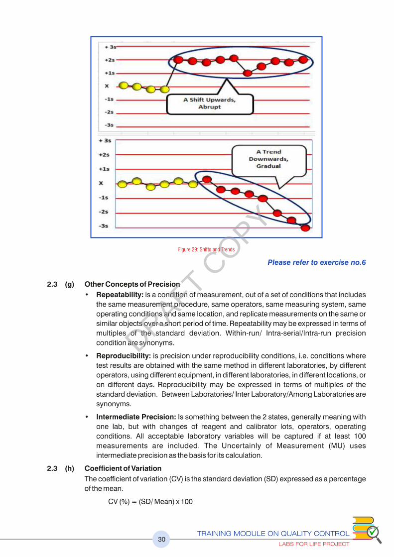
• Change in reagent formulation
• Change of reagent lot
• Major instrument maintenance
• Sudden change in incubation temperature (enzymes only)
• Change in room temperature or humidity
• Failure in the sampling system
• Failure in reagent dispense system
• Inaccurate calibration / recalibration
DRAFT COPY
TRAINING MODULE ON QUALITY CONTROL
LABS FOR LIFE PROJECT30
Please refer to exercise no.6
2.3 (g) Other Concepts of Precision
• Repeatability: is a condition of measurement, out of a set of conditions that includes
the same measurement procedure, same operators, same measuring system, same
operating conditions and same location, and replicate measurements on the same or
similar objects over a short period of time. Repeatability may be expressed in terms of
multiples of the standard deviation. Within-run/ Intra-serial/Intra-run precision
condition are synonyms.
• Reproducibility: is precision under reproducibility conditions, i.e. conditions where
test results are obtained with the same method in different laboratories, by different
operators, using different equipment, in different laboratories, in different locations, or
on different days. Reproducibility may be expressed in terms of multiples of the
standard deviation. Between Laboratories/ Inter Laboratory/Among Laboratories are
synonyms.
• Intermediate Precision: Is something between the 2 states, generally meaning with
one lab, but with changes of reagent and calibrator lots, operators, operating
conditions. All acceptable laboratory variables will be captured if at least 100
measurements are included. The Uncertainly of Measurement (MU) uses
intermediate precision as the basis for its calculation.
2.3 (h) Coefficient of Variation
The coefficient of variation (CV) is the standard deviation (SD) expressed as a percentage
of the mean.
CV (%) = (SD/ Mean) x 100
Figure 29: Shifts and Trends
DRAFT COPY
TRAINING MODULE ON QUALITY CONTROL
LABS FOR LIFE PROJECT31
The CV is used to monitor precision. When a laboratory changes from one method of
analysis to another, the CV is one of the elements that can be used to compare the precision
of the methods. As SD is expressed as a percent, it is easier to compare method imprecision
in CVs. The Allowable CV limits are defined in several published documents like BV Values
and CLIA Proficiency Limits. A suggested guideline is that, for CLIA values, 25% of the values
should be used for repeatability and 33% for intermediate precision. In the CLIA chart given
below, glucose Proficiency values are given as 10%. So the lab may choose to use 2.5% for
repeatability and 3.3% for Intermediate Precision. BV values may be used as such.
Please refer to exercise no.7
2.4 New Lot QC
2.4 (a) Establishing the Value of the Mean for a New Lot of QC Material Labs for Life QC
Tool: Parallel testing of QC
The practice of using the Manufacturer stated mean and SD can have a detrimental effect on
the patient reporting if the set values are incorrect or inappropriate. Therefore, new lots of a
quality control material should be analyzed for each analyte of interest in parallel with the lot
of control material in current use Ideally a minimum of at least 20 measurements should be
made on separate days when the measurement system is known to be stable, based on QC
results from existing lots. If the desired 20 data points from 20 days are not available,
provisional values may have to be established from data collected over fewer than 20 days.
Possible approaches include making no more than four control measurements per day for
five different days. Sampling from at least a few reconstituted vials will include any errors of
reconstitution. For liquid stable quality control products, fewer bottles may be required,
since such materials are expected to exhibit less vial to vial variation. When an opened bottle
of QC material will be used for more than one day, the same bottle should be assayed on
several days to allow analyte stability to be reected in the mean value. Also note that the
recommendation for a minimum of 20 days is intended to enable day to day sources of
variability in the measurement procedure to be reasonably represented in the mean value.
2.4 (b) Establishing the Value of the Standard Deviation for a New Lot of QC Material
If there is a history of quality control data from an extended period of stable operation of
the measurement procedure, the established estimate of the standard deviation can be
used with the new lot of control material, as long as the new lot of material has similar
target levels for the analyte of interest as for previous lots. The estimate of the standard
deviation should be reevaluated periodically.
If there is no history of quality control data, the standard deviation should be estimated,
preferably with a minimum of 20 data points from 20 separate days. The analyte stability
after opening a control product should also be considered, and the same bottle tested on
sequential days to include this source of variability in the estimate of SD. This initial
standard deviation value should be replaced with a more robust estimate when data from
a longer period of stable operation become available.
Estimates of the standard deviation (and to a lesser extent the mean) from monthly
control data are often subject to considerable variation from month to month, due to an
insufficient number of measurements (e.g., with 20 measurements, the estimate of the
standard deviation might vary up to 30% from the true standard deviation; even with 100
measurements. the estimate may vary by as much as 10%).More representative
estimates can be obtained by calculating cumulative values based on control data from
DRAFT COPY

TRAINING MODULE ON QUALITY CONTROL
LABS FOR LIFE PROJECT32
longer periods of time (e.g., combining control data from a consecutive six-month period
to provide a cumulative estimate of the standard deviation of the measurement
procedure). This cumulative value will provide a more robust representation of the effects
of factors such as recalibration, reagent lot change, calibrator lot change, maintenance
cycles, and environmental factors including temperature and humidity. Care should be
taken to ensure that the method has been stable and the mean has not been drifting
consistently lower or consistently higher over the six-month periods being combined, for
example due to degradation of the calibrator or control material.
An alternate method is to use the cumulative CV% and the mean obtained to arrive at an
attainable and defendable SD.Please refer to exercise no.2
2.4 (c) Having the Right Control Chart
Quality control procedures should be capable of detecting measurement errors at an
appropriately high rate (P ed > 90%) with minimum false accepts (an outlier accepted
because the chart did not ag it as an outlier) and minimum false rejections (P fr < 5% )(a
valid run rejected because the chart
agged it as an outlier), based on the
character ist ics of the part icular
analytical procedure being monitored
and the relevant medical requirements
for assay quality. To this end, it is
important to set the right Mean and
Standard Deviation on the chart.
In this graph assume that the SD (2) and
mean (84) are correctly assigned. Data
point “2” is 1:2s, data point “6” is 1:3s
and data point “12”is 1: 2s.
The same data points as in the earlier
graph, plotted with the mean of 82. This
wrong plotting, results in false rejects at
data points “2 & 12” and false accept at
data point “6”.
Thus a wrong mean assignment can
result in wrong interpretation of LJ graph.
Similarly wrong SD can also result in
false accepts and rejects. See figure 30.
See the violation of 68-95-99 rule, in both
cases, invalidating the SQC concept
altogether.
In the upper graph, the SD is too narrow
(1). This results in false rejection of many
values.
In the lower graph, the SD is too wide (4).
This results in false acceptance of many
values.
Figure 30: Importance of assigning mean & SD correctly on LJ graphs
Please refer to exercise no.9
DRAFT COPY

TRAINING MODULE ON QUALITY CONTROL
LABS FOR LIFE PROJECT33
2.5 Total Error ( TE)
2.5 (a) Total Error ( TE)
TE is evaluating the combination of errors. Total error combines bias and imprecision to
quantify the largest variation from the true or target value. Total analytical error is a useful
metric both to assess laboratory assay quality and to set goals. The common evaluation
methods are:
Direct Estimation
Indirect Estimation: (Discussed here)
Simulated Estimation
Indirect Estimation is by combining imprecision (SD) and average bias in the equation:
Total analytical error = SE (bias) + RE (1.65 * imprecision). Total Error thus will decrease if
the SE component (Bias) of RE component (SD) decreases and vice versa. It provides a
simple, cost effective method for evaluating performance.
2.5 (b) Target Value / True Value
Target Value may be obtained from
1) Inter-laboratory comparison programs of the QC manufacturer. Good QC providers
give monthly as well as cumulative means. The cumulative means are robust values
and will give very good anchoring as the true value
2) Manufacturer assigned mean
3) Long term lab mean provided the QC lot has been running for a considerable duration
OPTIMIZING THE PERFORMANCE OF QC PROCEDURES: 3rd AND 4th GENERATION QC
DRAFT COPY

TRAINING MODULE ON QUALITY CONTROL
LABS FOR LIFE PROJECT34
2.5 (c) Systematic Error (SE) or Bias
Bias is the difference obtained by subtracting the target value from the lab mean value.
Bias has direction. If the mean is more than the target it is a positive number and if less, a
negative number. But for the sake of calculations, the absolute number has to be used.
Example: If the Target is 100, and the Mean is 95, the Bias is 95- 100= -5. The absolute
bias [bias] is 5. SE is the absolute bias. The Systematic Error or SE here is 5.
Please refer to exercise no.10
2.5 (d) Random Error (RE)
We have seen in the above discussion that errors in precision affect method performance
and is measured as SD or CV%. Random Error is computed imprecision. Analytical errors
need to capture the degree of randomness in a measurement. There are 6 SDs
(population of data points) covered under the Gaussian, 3 on each side of the mean. ± 3
SD captures 99.7% of the data points. ± 2 SD captures 95% and ± 1.65 SD captures
90% and ± 1 SD 68% of data points. It can be understood from the figure 32, 50% of the
population of data points (the half of the Gaussian between the target and the Mean, X-
bar) are already captured along with the bias. A 1.65 SD will capture 90% from both sides,
leaving out 5% on each tail. But since one side is already accounted for, 1.65 is now
effectively capturing 95% of the total randomness (figure 32 and figure 33). Most
analytical error calculations use 1.65 as the Z factor for capturing random error.
Figure 31: Concept of Total Error (Combination of Systematic and Random Errors)
DRAFT COPY

TRAINING MODULE ON QUALITY CONTROL
LABS FOR LIFE PROJECT35
Figure 32: Capturing random errors from a Gaussian. The rationale of using 1.65 as the Z factor.
Figure 33: Capturing TE from a Gaussian. 95 % of the error are detected by using 1.65 as a z factor
2.5 (e) The Z Factor
The Z Factor determines the portion of the
population of data points to be included in the
estimation of the TE. The common multipliers
with the SD are:
• 2, Commonly used for quick calculations
• 1.96, to include 97.5% probability
• 1.65, to include 95% probability
For example, using 1.96 as the Z factor, 97.5%
of the possible data points will fall within the TE
attributed. 2.5% of the possible error points will
not be captured. On a more practical note, 1.65
is used as the Z factor to capture 95% of the
randomness.
Figure 34: Z factor Probability Chart
Please refer to exercise no.11
DRAFT COPY

TRAINING MODULE ON QUALITY CONTROL
LABS FOR LIFE PROJECT36
2.6 Total Allowable Error
Knowing the Total Error in a system will be of
clinical use only if there is benchmarking for the
allowable error for that analyte. Hence in the Total
Quality Management system (TQM), the concept
of Total Allowable Error (TE ) is very significant. A
Hence we can say that there are 4 key numbers
required to proceed with the performance
evaluation quality specifications.
2.6 (a) Quality Requirements
Total Allowable Error (TE ) is the amount of A
error that can be tolerated without invalidating
the medical usefulness of the analytic result.
The concept of quality requirements is the
foundation for quality planning. Quality
requirements can help guide interpretation of
laboratory test results because they provide
perspective about variability of results within an
acceptable interval and potential significance
of abnormal findings. A commonly used quality
requirement is Total Allowable Error (TE ), which is derived from medically important A
analyte concentrations or clinical decision thresholds. A hierarchy of quality requirements
has been proposed, and the most stringent quality requirements are based on clinical
outcomes and clinical decision thresholds. Quality requirements may also be based on
data about biologic variation of an analyte (BV Values), analytical performance criteria of
Proficiency Testing guidelines (e.g., as mandated by CLIA ), Proficiency testing values,
and in the absence of any better published guidelines, Tonk’s rule or even current SD * 3.
These are explained below;
2.6 (b) Getting the TE values: Applying the Stolkholm HierarchyA
1) Medical Requirements:
Apart from a few analytes like HbA1C with a TE specified as as ± 6% by NGSP and A
Total Cholesterol ± 9%, HDL-C 13%, LDL-C 12%, Tryglyceride 15% specified by
NCEP, no other analyte has directly defined TE values.A
2) Biological Variation (BV) Values
The BV values have 3 categories,
Optimum, Desirable and Minimum
specifications. The optimum is the
most stringent and Minimum. the
most lenient. The labs are well
advised to find a TE that is A
defendable and attainable and
hence start with desirable and up-
grade or downgrade as possible.
Figure 35: The Four Key Numbers
Figure 36: Stockholm Hierarchy for TEA
Figure 37: A graphical representation of iIntra and Inter individual BV
DRAFT COPY
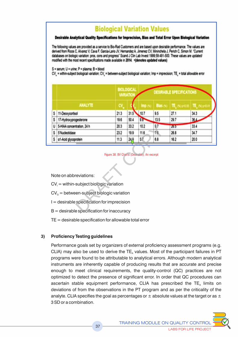
TRAINING MODULE ON QUALITY CONTROL
LABS FOR LIFE PROJECT37
Note on abbreviations:
CV = within-subject biologic variationI
CV = between-subject biologic variationG
I = desirable specification for imprecision
B = desirable specification for inaccuracy
TE = desirable specification for allowable total error
3) Proficiency Testing guidelines
Performance goals set by organizers of external proficiency assessment programs (e.g.
CLIA) may also be used to derive the TE values. Most of the participant failures in PT A
programs were found to be attributable to analytical errors. Although modern analytical
instruments are inherently capable of producing results that are accurate and precise
enough to meet clinical requirements, the quality-control (QC) practices are not
optimized to detect the presence of significant error. In order that QC procedures can
ascertain stable equipment performance, CLIA has prescribed the TE limits on A
deviations of from the observations in the PT program and as per the criticality of the
analyte. CLIA specifies the goal as percentages or ± absolute values at the target or as ±
3 SD or a combination.
Figure 38: BV Charts (Desirable); An excerpt
DRAFT COPY

TRAINING MODULE ON QUALITY CONTROL
LABS FOR LIFE PROJECT38
4) Using Proficiency Testing Results (past survey report)
In the absence of any guideline, the lab may use the survey reports from earlier PT
reports. As median values are used in PT reports, it will be less affected by outliers
and hence a good indicator of TE . An example is given above ( Figure 40 ). The CD 4 A
count reports complied shows a certain variation at each level, in SDs and CVs. A 3*
SD or CV may be applied as the TE . In the figure, if you take the average CV% it will A
be 5%. Three times this is 15%. This may be applied as the % TE . A count of 100 A
cells, an acceptable would be ± 15. Alternatively, the lab can use 3 times the
respective CV% against each level.
5) Tonk’s Rule: TE from Biological Reference IntervalsA
TE = 25% * BRI as per Tonk’s rules. Subtract the lower end of biological reference range A
from the upper end and divide by 4 for the absolute number or derive the percent with the
target value as the denominator. TE from reference intervals are also referred to in CLIA A
’88 rules which suggests 50% * BRI. This gives rise to considerable problems( See fig).
Besides, the reference intervals are lab defined, often revised. So it is ideal to avoid this.
Figure 41: CLIA proficiency limits; Excerpts
Figure 40: Estimating the TE using labs owns A
proficiency testing limits
Figure 39: CLIA limits defined in different ways percentage,+/- Absolute values, +/- SDs and combined
DRAFT COPY
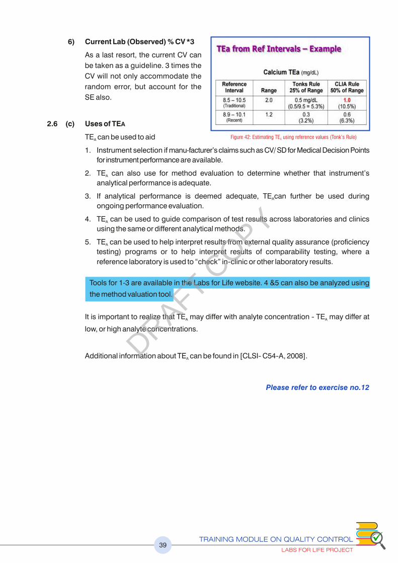
TRAINING MODULE ON QUALITY CONTROL
LABS FOR LIFE PROJECT39
6) Current Lab (Observed) % CV *3
As a last resort, the current CV can
be taken as a guideline. 3 times the
CV will not only accommodate the
random error, but account for the
SE also.
2.6 (c) Uses of TEA
TE can be used to aid A
1. Instrument selection if manu-facturer’s claims such as CV/ SD for Medical Decision Points
for instrument performance are available.
2. TE can also use for method evaluation to determine whether that instrument’s A
analytical performance is adequate.
3. If analytical performance is deemed adequate, TE can further be used during A
ongoing performance evaluation.
4. TE can be used to guide comparison of test results across laboratories and clinics A
using the same or different analytical methods.
5. TE can be used to help interpret results from external quality assurance (proficiency A
testing) programs or to help interpret results of comparability testing, where a
reference laboratory is used to “check” in�clinic or other laboratory results.
Tools for 1-3 are available in the Labs for Life website. 4 &5 can also be analyzed using
the method valuation tool.
It is important to realize that TE may differ with analyte concentration � TE may differ at A A
low, or high analyte concentrations.
Additional information about TE can be found in [CLSI� C54�A, 2008].A
Please refer to exercise no.12
Figure 42: Estimating TE using reference values (Tonk’s Rule)A
DRAFT COPY

TRAINING MODULE ON QUALITY CONTROL
LABS FOR LIFE PROJECT40
2.7 How Far Can the Mean Shift?
Once the TE and TEA are known, it is possible to assess the error margin. There are
different methods in which this can be done.
2.7 (a) Margin of Error
In the figures below, the observed mean is less than the True or Target Mean, rendering
the 1.65 SD or the outer edge of the Gaussian, towards the lower end of TEA. But if the
mean shifts further to the lower end as in figure below, 1.65 SD will touch and then cross
the lower limit of the TEA. This is the margin of error. In calculation, the margin for error
can be considered as TEA minus TE. If TE approaches TEA the margin for error
decreases. If TE exceeds TEA, the analytical system may be considered invalid .
2.7 (b) Critical Systematic Error (SEc) or �SEcrit
SEc is the size of the systematic error
that needs to be detected to maintain a
defined quality requirement. Critical
Systematic Error or SEc is the number
of SDs the mean can shift before
exceeding the TE . Thus SEc quantifies A
the Margin of Error in terms of a
measureable parameter, the SD. It
measures the multiples of SD that fit
within TE limits.A
The calculation of SEC also makes use
of the 4 key numbers
{(TEA- Absolute Bias) / SD} – 1.65
{(%TEA -% Bias)/ % CV}-1.65.
Where 1.65 is the Z factor and
represents the tail of the histogram that exceeds TE limit. By using this Z factor, we are
taking on a risk of 5% of wrong reports as acceptable.
THE FIFTH GENERATION QC: SETTING TOLERANCE LIMITS
Figure 43: (a) TE< TE , (b) TE>TEA A
Figure 44: Calculating SEc using the four key numbers & Z factor
DRAFT COPY

TRAINING MODULE ON QUALITY CONTROL
LABS FOR LIFE PROJECT41
2.7 (c) Sigma-metric = [(TE – Bias)/SD] = [(%TE -% Bias)/ % CV] = SEc + 1.65A A
We may consider the 1st generation QC as Levey-Jennings for manual methods and 2nd
generation QC for automated analyzers. Optimizing the performance of QC procedures
on the basis of quality required for the intended use of the test in terms of Total Error
observed for a particular method and definition of Total Allowable Error may be
considered the 3rd and 4th generation Qcs.
The 5th general QC emphasizes the need to define “tolerance limits” to describe intended
use, set a goal of 6-sigma for “world class quality,” and provides a uniform way of describing
quality in terms of defects, defect rates, defects per million (DPM), and the sigma-scale itself.
A world class or Six Sigma performance makes less than 3.4 defects per million
operations. ISO mandates that labs capture their quality indicators as % Yield, % Defects,
Defects per Million Occasions (DPMO) or Sigma. QC monitoring is by far, the most vital
Quality Indicator of a lab. A “sigma-metric QC selection tool” readily evolved from an
earlier “critical-error” tool and was eventually included in the CLSI C24A3 guidance for
“Statistical Quality Control for Quantitative Measurements”. Thus, standard QC planning
tools became available in the forms of manual tools, as well as computer programs.
A six sigma test can fit in 6 SDs on either side of the mean. This means there is no bias and
the degree of dispersion or imprecision is stable. In figure 45, see the first picture. This is
Six Sigma performance where the chances of defects is < 3.4/ million. In the second picture, the positive bias formation has compromised the margin the mean
can shift, and the Sigma number. Similarly a widening Gaussian due to imprecision can
also breach the limits leading to lower Sigma. Deriving the sigma metric for an analysis again combines the 4 Key Quality Numbers; Mean,
SD, Target and TE into one statistic. It benchmarks the performance of the measurement A
procedure in relationship to the quality required (i.e. Six Sigma ). Knowing the Sigma
performance of an analyte can be used to select appropriate control rules for a method. .
This is described in later sections.
Sigma= (TE - Absolute Bias) / SD A
or
Sigma= (%TE -% Bias)/ % CVA
Figure 45: Concept of Six Sigma in laboratoriesDRAFT COPY

TRAINING MODULE ON QUALITY CONTROL
LABS FOR LIFE PROJECT42
Figure 46: Sigma Performance matrix
2.8 QC Planning
The outlines of statistical QC may be evident from the above discussions. With the
knowledge of the basics, it is time to understand how to make a QC protocol for each
analyte depending on the method performance.
An effective QC design
1. Ensures quality performance by quickly detecting medically significant errors
(Percent Error Detection or P ed > 90%);
2. Generates few rule violations when there are no significant errors occurring
(Percent false rejection; P fr < 5%);
HOW TO USE ALL THESE INFORMATION IN YOUR LAB
Example:
Mean obs = 15 mmol/L
SD obs = 3 mmol/L
Target Value = 18 mmol/L
TE = 15 mmol/LA
Sigma = (15- 3)/ 3 = 4
Thus essentially the sigma metrics is an extension of SEc but can also be called a sigma-
metric, which is more easily understood in light of current interests in Six Sigma Quality
Management. Depending on the sigma performance on an anlayte, the monitoring rules
for that analyte can be modified. See Figure 46
Please refer to exercise no.13
DRAFT COPY

TRAINING MODULE ON QUALITY CONTROL
LABS FOR LIFE PROJECT43
3. Fewest number of control measurements per analytical run possible to save on
costs associated with;
- QC materials
- Reagents
- Consumables
4. Meets regulatory or accrediting body's requirements for number of
measurements per run.
2.8 (a) Percent False Rejects and Percent Error Detection
A simple Westgard rule system 1:2s (mean ± 2 SD) was used initially to monitor method
performance. However this rule has Percent False Rejection (P fr) of 4.5% in one control
measurement and 9% at 2 control measurements. This high false rejection rate would
render this rule a major waste of laboratory resources due to repeat analysis of controls
and samples resulting in an increase in the cost of the analytical process and a waste of
time and effort.
This type of waste can be avoided by designing a quality control procedure that is based
on the quality goal required clinically and the performance characteristics of each
test/analyzer. The laboratory's efforts would be focused on the analytes that require the
maximum control. The ideal IQC design should be derived for each individual test in a
multi-test system, selecting where possible the combination of the highest Percent Error
Detection (Ped) and the lowest Percent False Rejection (P fr).
2.8 (b) Using Multi-Rules: Seeing the Complete Picture.
A single-rule QC procedure uses a single criterion or single set of control limits, such as
either the mean plus or minus 2 standard deviations (2s) or the mean plus or minus 3s.
Multi-rules QC on the other hand, uses a combination of decision criteria, or control rules,
to decide whether an analytical run is in-control or out-of-control.
The N and R
N represents the total number of control measurements that are available at the time a
decision on control status is to be made. If 2 levels of (control levels)measurements are
available within one run, N=2. If three are available then, N=3.
R represents the number of runs
Example: If 2 levels of control measurements are available and two runs are available ,
N=2 & R=2 and the total available data points are 4 per day.
1:2s rule may be used as a warning to trigger application of the other rules, thus anytime a
single measurement exceeds a 2SD control limit, respond by inspecting the control data
using the other rules.
Within Run Errors: The Power of Daily Monitoring
• Stop and take corrective action if a single point exceeds a 3s limit.
• Stop and take corrective action if two levels of control exceed the same 2s limit.
DRAFT COPY

TRAINING MODULE ON QUALITY CONTROL
LABS FOR LIFE PROJECT44
• Stop and take corrective action if one point in the group exceeds a plus 2s limit and
another exceeds a minus 2s limit: R s This is a range rule that is meant only to be 4
applied within-run
Because N must be at least 2 to satisfy CLIA QC requirements, all these rules can be
applied within a run.
Across Run Errors: The Power of Periodic Review
Several rules like 4:1s, and 10x must be used across runs, within or across materials in
order to get the number of control measurements needed to apply the rules and to pick up
systematic errors. 2:2s can be used within and across runs. . In the case of 7 T, whenever
one level is trending, say, upward for 5- 6 times, and other level doing the same thing, it
should be investigated.
To reiterate, the advantages of multi-rules QC procedures are that false rejections can be
kept low while maintaining high error detection. This is done by selecting individual rules
that have very low levels of false rejection, then building up the error detection by using
these rules together
The power of daily monitoring PLUS The power of periodic review = 1 s/2 s/R s/4 s/10x3 2 4 1
For certain types of tests, notably hematology, immunoassay and blood gas, controls
tend to be run in three's, i.e., one low control, one middle control, and one high control.
For situations like this, it isn't practical to use the "Classic Westgard Rules"; those rules
were built for controls in multiples of 2. So when you're running 2, 4, 8 controls, use the
"classic" rules. When you're running 3 or 6 controls, use a set that works for multiples of
threes: In this case:
The power of daily monitoring PLUS The power of periodic review =1 s/2 of 3
3 s/R4s/ 3 s/12x2 1
2.8 (c) Length of Analytical Run
The length of an analytical run must be defined appropriately for the specific analytical
system and specific measurement procedure. In laboratory operations, control samples
should be analyzed during each analytical run to monitor method performance. The
length of the analytical run can be defined as an interval over which the risk (severity and
likelihood) of unexpected events that could impact precision and accuracy has been
mitigated to a tolerable level by virtue of the operational characteristics of the testing
system. The user should define the run length for the specific application in their own
laboratory because the operating conditions, workload, and application of the
measurement procedure in their laboratory may differ from nominal conditions evaluated
by the manufacturer.
The user should define the period of time or series of measurements within which
validation of the measurement procedure is important, based on the expected stability of
the measurement procedure, the number of patient samples typically being analyzed,
cost of reanalysis in the event of a QC failure, workow patterns, operator characteristics,
and the clinical impact of an undetected error condition existing for a period of time before
the next QC measurement(s). Stability of an analyte in patient samples is a consideration
DRAFT COPY

TRAINING MODULE ON QUALITY CONTROL
LABS FOR LIFE PROJECT45
because if an out-of-control condition is identified, then it is important that the QC
frequency will allow for the retesting of all potentially affected patient samples.
2.8 (d) Frequency of Control Measurements
Quality control samples must be analyzed at least once during each user-defined
analytical run length. Manufacturers of analytical systems or reagents may recommend
the number of quality control specimens and their location within the run. However,
manufacturers' recommendations should be used as guidelines and the frequency of QC
measurement should be established by the laboratory considering the factors outlined
later. The frequency and location of control samples should reect actual test system
performance and application at the site of testing.
2.8 (e) Location of Control Samples
The user should determine the location of control samples within a run, keeping in mind the
principle that quality control results should be evaluated before reporting patient results from
the run. The location of control samples should consider the type of analytical process, the
kinds of errors that might occur, and the protocol for reporting patient results. For example, if
an analytical run corresponds to a discrete batch of samples, the controls might be located
at the beginning and the end of the run to detect shifts, might be spaced evenly throughout
the batch to monitor drift, or distributed randomly among the patient samples to detect
errors. In any case, the QC results would be evaluated before patient results are reported.
For a high-volume analyzer that continuously produces test results, an appropriate
analytical run might be defined as a certain interval of time, then QC samples would be
analyzed and evaluated at the beginning of a run and then again as each run (i.e. ., the next
time interval or defined number of samples) occurs. If a quality control fault is detected,
results reported since the previous quality control event should be reviewed.
CAUTION: Routine placement immediately after calibration materials may give falsely
low estimates of analytical imprecision and will not provide any estimate of shift or drift
during the run.
2.8 (f) Developing a QC Plan
As explained earlier to come to the sigma-metrics, they 4 key numbers should be
available, the precision (SD/ CV) and accuracy (Observed Mean and Target Value) and
TE . Calculate the SEc and Sigma. It is important to have internal QCs with target values A
near Clinical Decision Points.
Define the quality required for each test, then assess the probabilities for false rejection
(P fr) and error detection (P ed) of the different candidate QC procedures on the Rule
Selection power graph. Aim for 90% error detection (P ed of 0.90 or greater) and 5% or
less false rejections (P fr of 0.05 or less).
Aim for 90% detection of medically important errors,
5% or less false rejections
DRAFT COPY

TRAINING MODULE ON QUALITY CONTROL
LABS FOR LIFE PROJECT46
To recap, use the following steps are suggested to develop an optimum QC plan
1. Define the quality that is needed for each test.
a. Know the performance of your method (CV, bias).
b. Get target value and Total Allowable Error from the best possible source.
c. Calculate the SEc and Sigma-metric of your testing process.
2. Decide on the rules to be applied to each analyte from the Rule Selection Power
Graph; Single Rule/ Multi rules.
3. Decide the number of controls measurements(N) and (R), number of runs of each QC
a. Use single-rule QC procedures and minimum number of control measurements
(N) & (R) for methods with high performance
b. Use single-rule QC procedures and moderate number of control measurements
(N) & (R) for methods with moderate to high performance
c. Use multirule QC procedures for methods with moderate to low performance
4. Define explicitly the application and interpretation of rules within and across materials
and runs
5. Interpret multirule to help indicate the occurrence of random error or systematic error.
2.8 (g) Tools to Use to Determine the Appropriate Control Rule(s)
If medically important errors can be detected 90% of the time (i.e., probability of error
detection of 0.90 or greater), then a single rule QC procedure is adequate. If 90% error
detection cannot be provided by a single rule QC procedure, then a multi-rules QC
procedure should be considered. In general, single rule QC procedures are adequate for
highly automated and very precise chemistry and hematology analyzers. However, the 2s
control limits or the 1:2s control rule should be avoided to minimize waste and reduce
costs. Earlier generation automated systems and manual methods will often benefit from
the improved error detection of multi-rules QC procedures.
There are many tools available to understand the rule(s) that should be used to alert you
to a significant error. The tools include power function graphs such as Sigma-Metric Rule
Selection Tool, critical-error graphs, QC Selection Grids, charts of operating
specifications (OP Specs chart), and the QC Validator, Westgard advisor by Bio-Rad, Opt-
mizer and EZ Rules .
In this manual, Sigma Metric Rule selection tool will be explained as it tis the tool
described in CLSI guidelines.
2.8 (h) Using the Sigma Metric Rule/Rules Selection Tool
This tool is a power function graph that shows the probability for rejection vs. the size of
the error for different QC rules and numbers of control measurements. The key to this tool
is the critical systematic-error (SEc) that needs to be detected by the QC procedure. The
rule selection depends on the quality required for the test and the precision and accuracy
observed for the measurement procedure. The critical systematic error is shown on the x-
DRAFT COPY

TRAINING MODULE ON QUALITY CONTROL
LABS FOR LIFE PROJECT47
axis at the bottom of the graph, the sigma-scale is shown at the top of the graph, and the
probability for error detection and probability of false rejection is shown on the y-axis. The
vertical lines represent measurement procedures having 3-sigma, 4-sigma, and 5-sigma
performance. The key at the right identifies the QC procedures. The curves in the graph,
left to right (1-8), match the list in the key, left to right (1-8). Pfr, probability for false
rejection; N, total number of control measurements; R, number of runs to which the QC
procedure is applied. Full formats of Tool selection graphs are given as annexure
number 4 A & B
The steps to be followed are:
1) Locate calculated sigma-value on Sigma-metrics graph.
2) Draw vertical line to intersect power curves.
3) Locate the point at which any of the 8 graphs cross the 0.9.
4) Select QC procedure corresponding to the number of that graph.
5) This set of rules provides Ped of 0.90 or 90% error detection.
In the example below, a SEc of 2.5 (Sigma 4.15) is being evaluated for appropriate QC
rules. The graph that intersects at 0.9 or 90% closest is graph number 3. (Please note
graphs 3 and 4 crossing over near 0.6 of the Y axis). The set of rules appropriate for Graph
3 is: 13s/22s/R4s/41s, N4 and R1. This means multirules as stated above, for 4 controls
available at each run, for 2 runs, and a false rejection of 0.03 or 3%.
Figure 47: Technique for using Sigma rule selection tool for QC rules in the lab
DRAFT COPY
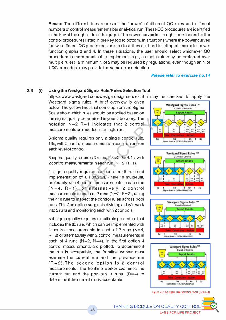
TRAINING MODULE ON QUALITY CONTROL
LABS FOR LIFE PROJECT48
Recap: The different lines represent the "power" of different QC rules and different
numbers of control measurements per analytical run. These QC procedures are identified
in the key at the right side of the graph. The power curves left to right correspond to the
control procedures listed in the key top to bottom. In situations where the power curves
for two different QC procedures are so close they are hard to tell apart; example, power
function graphs 3 and 4. In these situations, the user should select whichever QC
procedure is more practical to implement (e.g., a single rule may be preferred over
multiple rules); a minimum N of 2 may be required by regulations, even though an N of
1 QC procedure may provide the same error detection.
Please refer to exercise no.14
2.8 (i) Using the Westgard Sigma Rule/Rules Selection Tool
https://www.westgard.com/westgard-sigma-rules.htm may be checked to apply the
Westgard sigma rules. A brief overview is given
below. The yellow lines that come up from the Sigma
Scale show which rules should be applied based on
the sigma quality determined in your laboratory. The
notation N=2 R=1 indicates that 2 control
measurements are needed in a single run.
6-sigma quality requires only a single control rule,
13s, with 2 control measurements in each run one on
each level of control.
5-sigma quality requires 3 rules, 1:3s/2:2s/R:4s, with
2 control measurements in each run (N=2, R=1).
4 -sigma quality requires addition of a 4th rule and
implementation of a 1:3s/2:2s/R:4s/4:1s multi-rule,
preferably with 4 control measurements in each run
( N = 4 , R = 1 ) , o r a l t e r n a t i v e l y, 2 c o n t r o l
measurements in each of 2 runs (N=2, R=2), using
the 41s rule to inspect the control rules across both
runs. This 2nd option suggests dividing a day’s work
into 2 runs and monitoring each with 2 controls.
<4-sigma quality requires a multirule procedure that
includes the 8x rule, which can be implemented with
4 control measurements in each of 2 runs (N=4,
R=2) or alternatively with 2 control measurements in
each of 4 runs (N=2, N=4). In the first option 4
control measurements are plotted. To determine if
the run is acceptable, the frontline worker must
examine the current run and the previous run
( R = 2 ) . T h e s e c o n d o p t i o n i s 2 c o n t r o l
measurements. The frontline worker examines the
current run and the previous 3 runs. (R=4) to
determine if the current run is acceptable.
Figure 48: Westgard rule selection tools (EZ rules)
DRAFT COPY

TRAINING MODULE ON QUALITY CONTROL
LABS FOR LIFE PROJECT49
2.8 (j) Using the OPSpecs Tool
Relationship between the quality requirement for the test, the precision and accuracy
observed for a method, and the rejection characteristics for different control rules and
numbers of control measurements are used to develop OpSpecs Chart. “Normalized”
OPSpecs charts minimize the number of charts when the observed imprecision and bias
are expressed as a percentage of the quality requirement. Online OpSpecs tools are
available for rule selection.
An OpSpecs chart showing acceptability
of the method based on sigma metrics. In
practice, the normalized OPSpecs charts
are scaled from 0 to 100% on the y-axis and
0 to 50% on the x-axis and the x-coordinate
and y-coordinate are expressed as a
percentage of the quality requirement
This example of a methods decision chart
shows allowable total error. Allowable
inaccuracy (% bias) is plotted on the y-axis
versus allowable imprecision (% CV) on
the x-axis. Diagonal lines represent, from
left to right, 6-sigma, 5-sigma, 4-sigma, 3-
sigma, and 2-sigma quality. Operating
point (A) shows a method having a bias of
1.0% and a CV of 1.5% that demonstrates
4-sigma quality.
Figure 49: OPSpecs scale for Lab QC rule selection
User plots a normalized operating point
that displays method performance as a
percentage of the quality requirement of
the test. An acceptable QC procedure is
o n e w h o s e o p e r a t i n g l i m i t s f o r
inaccuracy and imprecision include the
user’s operating point, i.e., that point
falls below the line, whose rules and
total number of control measurements
are shown in the key at the right.The
lines below the 3.0 sigma line represent
different SQC procedures, as identified
in the key at the right.
DRAFT COPY

TRAINING MODULE ON QUALITY CONTROL
LABS FOR LIFE PROJECT50
2.8 (k) When Sigma and SEc are low
When an analyte shows <4 sigma, the lab must take special care for risk analysis.
a) SQC Measures
Multi rules
Look-back to previous runs
Increase N: Number of Qcs
Increase R: Number of QC runs
b) Non SQC Methods
Staff with special training to be deployed for low sigma tests
Increase the number of supervision
2.9 Uncertainty of Measurement (Mu)
2.9 (a) Why and What is MU?
Clinicians compare most measurement results with reference values and with previous
results from the same patient. Results should therefore be reliable and accurate. But the
inherent errors could be misleading, rendering ongoing monitoring by clinicians difficult.
The MU approach focuses on identifying the dispersion of results that might have been
obtained for an analyte if a sample had been measured repeatedly instead of once. CLSI
defines MU as associated with the result of a measurement, that characterizing the
dispersion of the values that could reasonably be attributed to the analyte. To do this, the
MU approach uses available data about repeated measurements from a given measuring
system to define an interval of values within which the true value of the measured analyte
is believed to lie, with a stated level of confidence. The parameter may be, for example, a
standard deviation. The term measurement uncertainty tends to give the wrong
impression, as it is actually a quantitative indication of the level of confidence, or
belief, the laboratory has about the quality of a result.
ISO 15189 mandates the determination of measurement uncertainty of all measurement
procedures. All types of measurement that have a magnitude expressed as a number and
a reference need to define the MU as per ISO.
DRAFT COPY

TRAINING MODULE ON QUALITY CONTROL
LABS FOR LIFE PROJECT51
2.9 (b) Sources that Contribute to Uncertainty
• Biological within-subject Biological Variation stress, drugs,
• Pre-analytical: including sampling, sample preparation and sample portion and
sample transport and selection among
• Analytical: calibrators and reference materials, input quantities, equipment used,
changes of operator, water quality and environmental conditions leading to random
and systematic errors (RE + SE)
• Post-analytical: such as errors of transcription
As per ISO the Measurement Uncertainty need to factor in only the uncertainty
components associated with analytical errors.
2.9 (c) Deriving Uncertainty of Measurement
Ideally the MU should capture all the elements of uncertainty. But as said earlier, in
practice, MU is concerned with only analytical uncertainty. In the analytical errors, unlike
TE, MU is not concerned with measurement error, but is concerned only with reporting to
clinicians. All components of analytical uncertainty, including those arising from
systematic effects, such as components associated with corrections and reference
standards, contribute to the dispersion should ideally be included. However, the
calculations of MU assumes that the bias cannot be estimated correctly and hence is not
considered in the estimate of MU. The MU approach assumes that known bias is
eliminated or minimized e.g. by re-calibration. Further, just as a bias value cannot be
exactly known, bias cannot be completely eliminated. The MU approach recognizes that
the value used for bias correction has an associated uncertainty, being the combination of
the uncertainty of the reference value itself.
Thus some of the components like imprecision of the measuring system may be
evaluated from the statistical distribution of the results of series of measurements and can
be characterized by standard deviations. The other components, like imprecision of the
bias value used if bias was eliminated or minimized may also be characterized by
standard deviations as expanded uncertainty. Since it is rarely possible in practice due to
limited time and resources, the extended uncertainty of a measurement result is usually
evaluated with a mathematical model using the law of propagation of uncertainty.
2.9 (d) Combined Standard Uncertainty (µc)
As the best material that lends itself to repeated analysis is Internal Quality Control, ISO
suggests the IQC values form the basis of MU determination. The mean value and SD is
calculated for each level of QC used for a given measurement procedure over a sufficient
time to encompass as many routine procedure changes as possible; at least 30 values is
be adequate for an initial MU estimate. The parameter of MU is 1 SD (standard
measurement uncertainty, symbol µ). Because the SD of the QC reects the combined
effect of all the individual uncertainties arising within the measuring system, the SD can be
considered as the combined standard uncertainty (µc) for patients results around the
mean value of the particular QC.
DRAFT COPY

TRAINING MODULE ON QUALITY CONTROL
LABS FOR LIFE PROJECT52
2.9 (e) Expanded Uncertainty (U)
Since ±1 SD covers only ~68 % of the dispersion of obtained QC values, the uncertainty
is widened by applying a coverage factor (k) to provide an expanded measurement
uncertainty (symbol U). Usually k = 2 is chosen, to provide a more useful 95.5 %
coverage of the dispersion of results. Assuming such a dispersion also applies to patients
results, then a result could be in the form x ± y (95 % confidence), where x is the result
obtained from the test and y = 2 SD (i.e. 2 x µc = U).
If several levels of QC are used the MU should be calculated for each, and a judgment
made as to whether they are sufficiently different to warrant their use with patient results
that fall in the range considered to be covered by each QC level.
The expanded UM may also be expressed as a percentage at that level, which is the
CV%* 2.
2.9 (f) Coverage factors and confidence limits
Applying the following coverage factors will offer the corresponding confidence limits.
• k=1.00 (68.27%)
• k=1.00 (64.90%)
• k=1.00 (96 .95%)
• k=2.00 (95.45%)
• k=2.00 (58 99%)
• k=3.00 (99.73%)
2.9 (g) Intermediate Precision
Using Intermediate Precision capturing the variables associated with changes in reagent
and calibrator lots, operators, operating conditions. 100 data points will be the optimum
number used to express UM. A periodic review of the UM is warranted.
Measurement procedures do not permit components (e.g. sampling/reagent probes,
water quality, water-baths, ambient temperature etc.) to be individually studied to
ascertain their uncertainty for the combined effect on the variability on measurement
results. The QC data used for MU calculations is obtained over a period of time sufficient to
capture variability due to routinely occurring changes in the measuring system e.g. reagent
and calibrator batch changes, different operators, routine maintenance etc. i.e. intermediate
reproducibility or intermediate precision. In measurement procedures that are sufficiently
robust that imprecision levels are stable between reagent batches, a combined SD may be
used. Adequate data (>100 results) takes longer to obtain for infrequently performed
measurement procedures, in which case interim calculations are appropriate, but in any
case, including new procedures, a minimum 30 QC results is required before an
approximate Gaussian distribution of data points can be reasonably assumed. Thereafter,
as QC results accumulate, the imprecision should be regularly re-calculated until the SD is
stable at the same number of decimal places used for reported results.
For more on MU calculation please see https://www.westgard.com/hitchhike-mu.htm
DRAFT COPY
TRAINING MODULE ON QUALITY CONTROL
LABS FOR LIFE PROJECT53
2.9 (h) The Difference and Relation Between UM and TE
Though UM (Measurement Uncertainty) and TE (Total Error) are related concepts, the
UM does not include the concept of Bias as the assumption is that the True Value
cannot be known.
However, the purpose of calculating the UM is not to plan QC strategy but to make
the uncertainty known to the users of the lab. As per ISO 15189, upon request the lab
has to make the UM available to the users.
• TE provides an approximate worst case value for the error of a measuring system.
• TE is useful for setting upper limits of allowable error.
• MU is not concerned with estimating the total error of a measuring system.
• MU is concerned with estimating an interval of values within which the ‘true’ value
of a measured analyte is believed to lie, with a stated level of confidence.
• MU considers a single measurement result to be the best estimate of a true value,
and centers on it the dispersion of other values that could have been obtained if
the measurement had been repeated (usually with ~95 % confidence).
• MU is the appropriate approach for meaningfully comparing measurement
results with reference values and previous results of the same kind.
In summary, MU does not estimate error, but provides a quantitative estimate of where the
true value of a measured analyte is believed by the laboratory to lie, with a stated
confidence level. MU is therefore an essential parameter of the reliability of measurement
results.
2.9 (i) Reporting Conventions
• 100 mg/dL is the result and if 3 is the SD +/- 3 Defines the result and Combined
Standard Uncertainty (µc)
• 100 mg/dL +/- 6 – Defines the result and the expanded uncertainty (U with k=2)
• 100 mg/dL +/- 6 mL at 95% confidence level. – Defines the expanded uncertainty at
the specified confidence interval
2.10 Average of Normals (AON) & Bull’s Algorithm
AON method is based on the principle that mean value of all normal results uctuate between
well-defined limits. AON method detects only systematic error. This method is mostly used
for biochemistry analyzers.
The laboratory collects data for an analyte from a fixed number of healthy persons. Its mean
value and standard deviation is calculated. This value will be used as control value.
Bull had determined that some hematological parameters have very small biological
variation (CVg) resulting in their mean value remaining steady. Bull applied his idea in
erythrocyte indexes (MCV, MCH, MCHC) at the beginning, but today his algorithm is used for
the majority of hematological parameters. This is an effective way of determining equipment
performances for systematic errors.
In Bull’s algorithm a moving average of all tests done is considered as the anchor and
determiner of equipment performance instead of a single QC mean value. The moving
DRAFT COPY
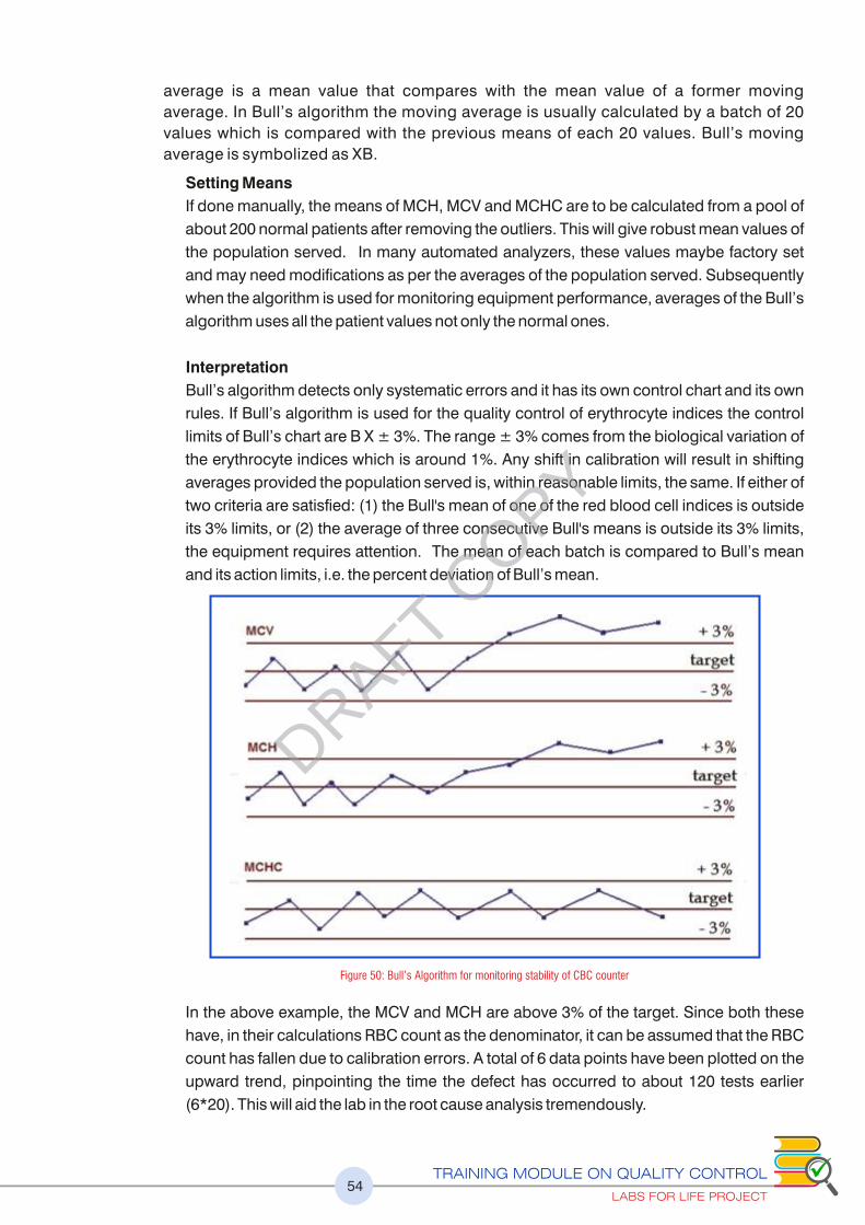
TRAINING MODULE ON QUALITY CONTROL
LABS FOR LIFE PROJECT54
average is a mean value that compares with the mean value of a former moving
average. In Bull’s algorithm the moving average is usually calculated by a batch of 20
values which is compared with the previous means of each 20 values. Bull’s moving
average is symbolized as XB.
Setting Means
If done manually, the means of MCH, MCV and MCHC are to be calculated from a pool of
about 200 normal patients after removing the outliers. This will give robust mean values of
the population served. In many automated analyzers, these values maybe factory set
and may need modifications as per the averages of the population served. Subsequently
when the algorithm is used for monitoring equipment performance, averages of the Bull’s
algorithm uses all the patient values not only the normal ones.
Interpretation
Bull’s algorithm detects only systematic errors and it has its own control chart and its own
rules. If Bull’s algorithm is used for the quality control of erythrocyte indices the control
limits of Bull’s chart are B X ± 3%. The range ± 3% comes from the biological variation of
the erythrocyte indices which is around 1%. Any shift in calibration will result in shifting
averages provided the population served is, within reasonable limits, the same. If either of
two criteria are satisfied: (1) the Bull's mean of one of the red blood cell indices is outside
its 3% limits, or (2) the average of three consecutive Bull's means is outside its 3% limits,
the equipment requires attention. The mean of each batch is compared to Bull’s mean
and its action limits, i.e. the percent deviation of Bull’s mean.
In the above example, the MCV and MCH are above 3% of the target. Since both these
have, in their calculations RBC count as the denominator, it can be assumed that the RBC
count has fallen due to calibration errors. A total of 6 data points have been plotted on the
upward trend, pinpointing the time the defect has occurred to about 120 tests earlier
(6*20). This will aid the lab in the root cause analysis tremendously.
Figure 50: Bull’s Algorithm for monitoring stability of CBC counter
DRAFT COPY

TRAINING MODULE ON QUALITY CONTROL
LABS FOR LIFE PROJECT55
2.11 Radar/ Spider Charts
A Radar Chart is a graphical method of displaying multivariate data in the form of a two-
dimensional chart of three or more quantitative variables represented on axes starting from
the same point.
Some CBC analyzers employ radar graph to denote QC and XB data.
The data of QC values from the selected QC file is displayed on the radar chart. If there are
no plots it means that no run are available in the selected QC file. Only the outline and
parameter names are displayed.
Parameter names are displayed as text on an outer circle. If the latest QC data falls outside
the QC limit values it displayed on radar chart.
For points which fall beyond the upper or lower limit, a red “X” is plotted on the upper or
lower limit. Data equals the target value: Plotted on the central line. (Blue line in the graph)
Data exceeds the upper limit: Plotted on the upper limit line as a red “X”.
Data falls below the lower limit: Plotted on the lower limit line as a red “X”.
In the example below, RBC is higher than acceptable and Hb is lower than acceptable and
are agged by red X. Other values are acceptable.
Multiple radar charts may be built in for parameters of QC and XB.
Inner line
Outer line
Blue Central line
Green irregular line
Lower limit value of QC
Upper limit value of QC
Target value
Latest QC data from the QC fileselected in the file list
Figure 51: Radar graph used in QC monitoring in Hematology Analyzers
DRAFT COPY

TRAINING MODULE ON QUALITY CONTROL
LABS FOR LIFE PROJECT56
2.12 Harmonization/ Comparability of Tests
Many labs use multiple equipment for the same tests. There could be differences in the
performance of each equipment. The traceability of the reference materials would be
different. The equipment may even have different method of testing. Thus if the laboratory
uses more than one measuring system where the measurements are not traceable to the
same reference material / reference method, or the biological reference interval are different,
it is essential to perform a comparability study between the systems and prove that there is
agreement in performance throughout appropriate clinical intervals. This is recommended
at least twice in a year using suitable statistical procedures such as Bland - Altman plot and /
or regression analysis. This kind of analysis explained in detail in subsequent sections.
Though not a standard procedure, this exercise may also be employed in ongoing method
evaluation in resource limited settings. If one equipment is adequately performance-
evaluated on an ongoing basis, this can be used as reference equipment and the other
similar equipment compared to this daily. An assessment of the difference percent may be
employed to evaluate the performance of the equipment. Labs for Life QC Tool:
Harmonization / Comparability of Tests
2.13. Conclusion: SQC
The discussions above give details of the Quantitative QC, from the point of purchase
through applications in daily monitoring using LJ graphs, assessment of Total Error and
Sigma-metrics and being used in planning of ongoing method performance and planning. It
also briey discusses the concept of Measurement Uncertainty and other statistical methods
for performance evaluation.
DRAFT COPY

TRAINING MODULE ON QUALITY CONTROL
LABS FOR LIFE PROJECT57
Learning Objectives
At the end of this chapters, the learners will be able to understand the
ISO requirements for proficiency testing (Inter-laboratory comparison)
Different mechanism for proficiency testing
Assessing acceptability of the proficiency testing reports
Frequency and scope of testing of some commonly used EQA in India (in
annexure)
CHAPTER 3: PROFICIENCY TESTING OR
EXTERNAL QUALITY ASSURANCE
“External Quality Assurance monitor the accuracy of the laboratory’s methods on an ongoing basis.
It enables the lab to compare itself with others using the same method for the same analyte.
Essentially EQA involves use of the same sample in several labs and comparing the lab’s results
with that of others performing the same test by the same method. Participation in EQA enhances
the confidence of the lab in its results. It also enhances the users’ confidence in the lab they use for
their tests.
3.1 ISO Requirements
Several terms are used interchangeably to denote External Quality Assurance processes.
ISO 15189: 2012, Clause 5.6.3 uses the terms Inter laboratory Comparisons (ILC) and
External Quality Assurance (EQA) synonymously. It mandates that the laboratory
participate in an ILC/EQA appropriate to the examinations and interpretations of the
examination results. It further says the laboratory understand the interpretations of the report
and do appropriate corrective actions whenever necessary.
The accreditation standard for ILC/EQA is 17043. The laboratory should strive to
participate in an ILC/EQA program accredited by or at least substantially fulfill the
relevant requirements of 17043.
ISO also mandates that the ILC/EQA samples should be integrated into the routine
laboratory testing process and not be treated as special category. It also requires to be
run by the same staff that runs tests. It also says that the ILC/EQA samples should be run just
once with no confirmatory run.
Also as per regulatory requirements, the labs are required to keep the raw data of
analysis such as equipment printouts of proficiency testing, for verification in audits
DRAFT COPY

TRAINING MODULE ON QUALITY CONTROL
LABS FOR LIFE PROJECT58
Kinds of External Quality Assurance
This module is referring to ILC/ EQA as of 3 of kinds:
• Proficiency testing or PT
• Inter Laboratory Comparison (ILC) program by peer group
• Split testing (by exchange of samples)
3.2 Proficiency Testing or PT
It is the testing of unknown samples from a common pool is sent to a laboratory by an
approved PT program provider. Most sets of PT samples are sent to participating
laboratories three or more times per year. After testing the PT samples in the same manner as
its patient specimens, the laboratory reports its sample results back to their PT program. The
program grades the results using some approved grading criteria and sends the laboratory
scores reecting how accurately it performed the testing.
3.2.1 PT Report Attributes
The following are the requirements that should be seen on PT reports
A. Analyte name
B. Units of reporting of a parameter
C. Survey sample ID
D. Reported results
E. N: the number of participating labs.
F. Mean
G. Expected Range
H. SD
I. SDI/Z score/other parameters for comparison
J. Grade/ Acceptability
The following figure shows an example. Analyte name, units of reporting, sample IDs,
reported results and N are circled for ease of understanding
Figure 52: Attributes of PT/EQA reports (1)
DRAFT COPY

TRAINING MODULE ON QUALITY CONTROL
LABS FOR LIFE PROJECT59
The above example shows a PT result for platelets. Please note the unit definition. In India,
platelets are generally expressed in Lakhs or Hundred Thousands (103) /uL.
In this example, one PT includes 5 levels to include several clinical decision levels. Reported
results and N are given.
The N
The N is the number of participating labs in the PT program. The providers may define and
compare (explained later) the participant lab’s result in several ways.
If N is too low, statistics may not be calculated for that peer group by the PT provider. The
higher the N, the better an estimate of the target value can be determined for that PT sample.
The higher the N, the more data points can be used to calculate the SD for the group. The
higher the N, the less impact aberrant results or incorrectly defined outliers will have on the
group’s SD and/or mean. At the least lowest minimum N of 10 is required. An N of 100 gives
very good anchoring of the mean. A 30 in is an acceptable good number.
• as part of all reports submitted for that analyte or;
• more specifically as part of the reports performed by the same method for that
anlayte or;
• most specifically, by the same method and equipment as the participant lab, for
that analyte;
• N is equally important in all the above scenarios
3.2.2 Acceptance Criteria
The Mean and the Range
The above table shows the range of the expected results as well as mean of all the
participants. The mean is the average results of all participants, after removing the outliers. In
a PT, the mean of all inliers is the best estimate of the true or expected value.
Figure 53: Attributes of EQA reports (2)
DRAFT COPY

Range can be determined by one of three ways
1) Target Value ± specified value (as in the above example, the specified value being the TE A
in units, at the target)
2) Percentage ± specified %
3) Multiple of PT group standard deviation (SD) ±specified 2 or 3 Sds
The range is calculated in the above example by deriving the TE at mean and adding and A
subtracting it from the mean. Acceptable performance criteria are defined by the service
provider and should be understood by the participant lab. The service provider is required to
tell the users the mechanism of assigning the acceptable range.
If 80% of the submitted results do not fall within the limits of acceptability, then no
results are graded.
3.2.3 Scoring Systems
This section explains a few scoring systems used by PT providers. A list of PT used in India is
also simultaneously incorporated as per their reporting system. A guideline on each
provider’s scope and sample frequency is also attempted. For more details, the reader is
advised to visit the corresponding sites.
3.2.3 (a) SDI (Standard Deviation Index) / Z score
The data from all the laboratories are usually analyzed to determine an overall average
and standard deviation for the group. The program will generally report your
performance relative to the group. The difference between your test results and the
overall average is often expressed by a standard deviation index, or SDI, which
expresses the difference in terms of the number of standard deviations from the overall
mean. Thus SDI/Z-score is a calculated value that tells how many standard deviations
the reported value is from the expected value for that material. It is calculated by taking
the difference between the reported value and the expected value, then dividing by the
standard deviation observed for that control material from the analyses in all
participant labs. For example, for reported value of 112 for an expected value of 100
and a standard deviation of 5, the SDI/Z-score is 2.4 [(112- 100)/5] denoting 2.4
standard deviation in the positive direction from its expected value
On a series of specimens, if you observe SDIs such as +1.5, +0.8, +2.0, +1.4, and +1.0
(all positive), this suggests that your method is generally running on the high side and is
biased, on average, by +1.3 SDI.
Difference between SDI and the Z-score.
They're basically the same thing, but the Z-score tends to be used more in Internal QC
programs to compare an individual QC result with the expected values for that
material, whereas the SDI tends to be used in external QC programs to compare the
performance of the lab with the overall mean for a defined comparative group or with
an established target value.
TRAINING MODULE ON QUALITY CONTROL
LABS FOR LIFE PROJECT60
DRAFT COPY
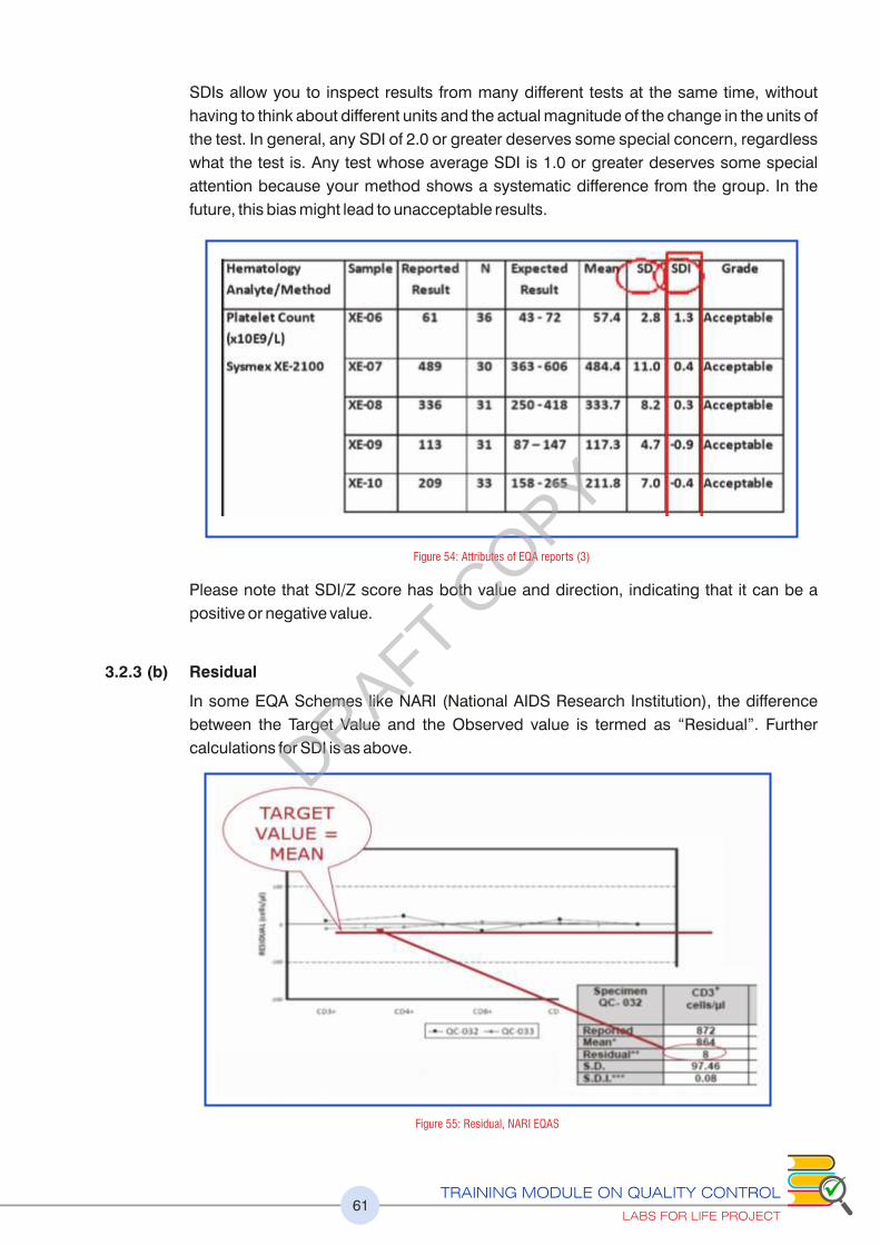
TRAINING MODULE ON QUALITY CONTROL
LABS FOR LIFE PROJECT61
SDIs allow you to inspect results from many different tests at the same time, without
having to think about different units and the actual magnitude of the change in the units of
the test. In general, any SDI of 2.0 or greater deserves some special concern, regardless
what the test is. Any test whose average SDI is 1.0 or greater deserves some special
attention because your method shows a systematic difference from the group. In the
future, this bias might lead to unacceptable results.
Please note that SDI/Z score has both value and direction, indicating that it can be a
positive or negative value.
3.2.3 (b) Residual
In some EQA Schemes like NARI (National AIDS Research Institution), the difference
between the Target Value and the Observed value is termed as “Residual”. Further
calculations for SDI is as above.
Figure 54: Attributes of EQA reports (3)
Figure 55: Residual, NARI EQAS
DRAFT COPY
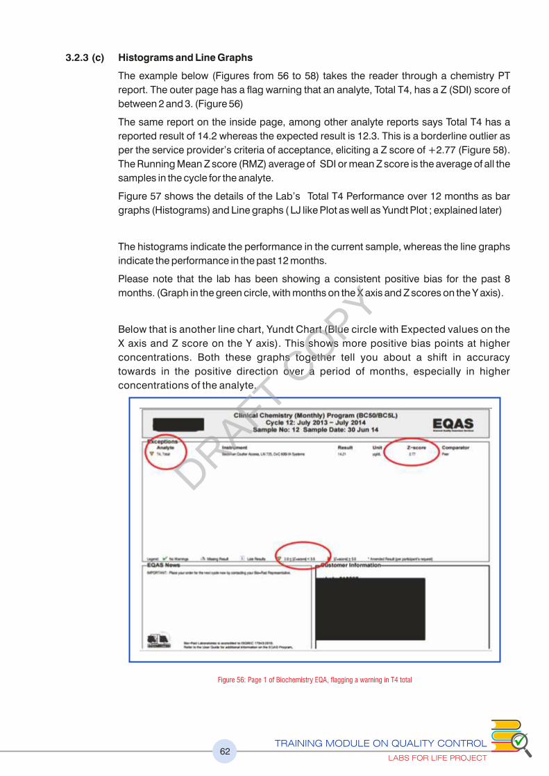
TRAINING MODULE ON QUALITY CONTROL
LABS FOR LIFE PROJECT62
3.2.3 (c) Histograms and Line Graphs
The example below (Figures from 56 to 58) takes the reader through a chemistry PT
report. The outer page has a ag warning that an analyte, Total T4, has a Z (SDI) score of
between 2 and 3. (Figure 56)
The same report on the inside page, among other analyte reports says Total T4 has a
reported result of 14.2 whereas the expected result is 12.3. This is a borderline outlier as
per the service provider’s criteria of acceptance, eliciting a Z score of +2.77 (Figure 58).
The Running Mean Z score (RMZ) average of SDI or mean Z score is the average of all the
samples in the cycle for the analyte.
Figure 57 shows the details of the Lab’s Total T4 Performance over 12 months as bar
graphs (Histograms) and Line graphs ( LJ like Plot as well as Yundt Plot ; explained later)
The histograms indicate the performance in the current sample, whereas the line graphs
indicate the performance in the past 12 months.
Please note that the lab has been showing a consistent positive bias for the past 8
months. (Graph in the green circle, with months on the X axis and Z scores on the Y axis).
Below that is another line chart, Yundt Chart (Blue circle with Expected values on the
X axis and Z score on the Y axis). This shows more positive bias points at higher
concentrations. Both these graphs together tell you about a shift in accuracy
towards in the positive direction over a period of months, especially in higher
concentrations of the analyte.
Figure 56: Page 1 of Biochemistry EQA, agging a warning in T4 total
DRAFT COPY

TRAINING MODULE ON QUALITY CONTROL
LABS FOR LIFE PROJECT63
Figure 57: Summary page showing all analytes with details of ranges and SDs, Z scores and RMZ etc.
Figure 58: The details of T4 in the last 12 cycles showing patterns of bias in the upper level in Yundt plot
The Comparator
To continue with the above figure, see
the red box which shows 3 comparators
• The current month’s report of 14.21 has
a +2.77 Z score in peer group
comparisons (Red Arrows)
• There are 2 more comparison groups
(Blue Arrow); “Your Mode and” “Your
Method”, the first denoting all the results
obtained, in this case for Total T4 in that
cycle (with N of 535) and the second, all
the Total T4 results done by CLIA method
but on many different equipment (N of
328), and the third your peer (same
method, same equipment), with an N of 39. Whereas the first 2 comparisons show a
better Z score, the third the more specific peer comparison shows a higher Z score.
Please note how the N reduces as the comparison mode becomes specific. However, 39
is still a robust N. These numbers must be taken into consideration as you evaluate your
PT report
• Quick reference bar graphs as histograms thus give visual assistance to the lab’s
performance with reference to the comparators.
Thus the best indicator of accuracy can be obtained by comparing with the same method
and equipment. The lab should understand the comparator in the program it is
participating in
Figure 59: Histograms with consensus mean & limits
DRAFT COPY

TRAINING MODULE ON QUALITY CONTROL
LABS FOR LIFE PROJECT64
3.2.3 (d) Cumulative Reports
Cumulative reports will also be made available by some providers giving a quick overview
of the long term, comprehensive performance of the lab, analyte wise. See below.
3.2.3 (e) The Target Score (TS) and %Deviation by Concentration Chart
TS allows participants to assess their performance at a glance.
The TS relates the %Deviation of the reported result from the Mean to a Target Deviation
for Performance Assessment (TDPA). TDPAs are set to encourage participants to achieve
and maintain acceptable performance. TDPAs are fit-for-purpose performance criteria
which are set taking guidance from ISO/IEC17043, ISO13528 and IUPAC. Target
Deviations for Performance Assessment are also used to calculate the Standard
Deviation for Performance Assessment (SDPA).
%Deviation by Concentration Chart is similar to the Yundt plot and enables rapid
assessment of concentration related biases. Biases at low or high concentrations can be
easily determined
3.2.3 (f) The Target Score (TS) Plot
%Deviation by Concentration Chart
This is in principle similar to the Yundt plot, with concentrations on the X axis and %
Deviation on the Y axis, allowing the lab to understand biases at specific concentrations
to enable calibrations and correction of the bias.
Figure 60: Cumulative reports: EQAS
DRAFT COPY

TRAINING MODULE ON QUALITY CONTROL
LABS FOR LIFE PROJECT65
3.2.3 (g) The VIS Scoring
The VIS or Variance Index Scoring is another scoring system used in India, especially in
CMC Vellore Biochemistry EQAS.
The VIS system was first proposed by the United Kingdom National Quality Control
Scheme (UKNEQUAS). It uses CCV (Chosen Co-efficient of Variation) & DV
(Designated Value/ Expected value) used to calculate VIS, CCV being the Allowable
Limit of Error for an analyte (TE ) (Please see Table below), the sum of both imprecision A
and bias. This method has been set & recommended by WHO after studying the
performance of many Indian labs.
The calculation is done in 2 steps.
1) % Variation [%V] = {(Reported Value – Expected value)/ Expected Value} *100
2) Variance Index = (% V/ CCV) X 100
Figure 61: Target Deviation for Performance Management
Figure 62: Percent deviation plotDRAFT COPY
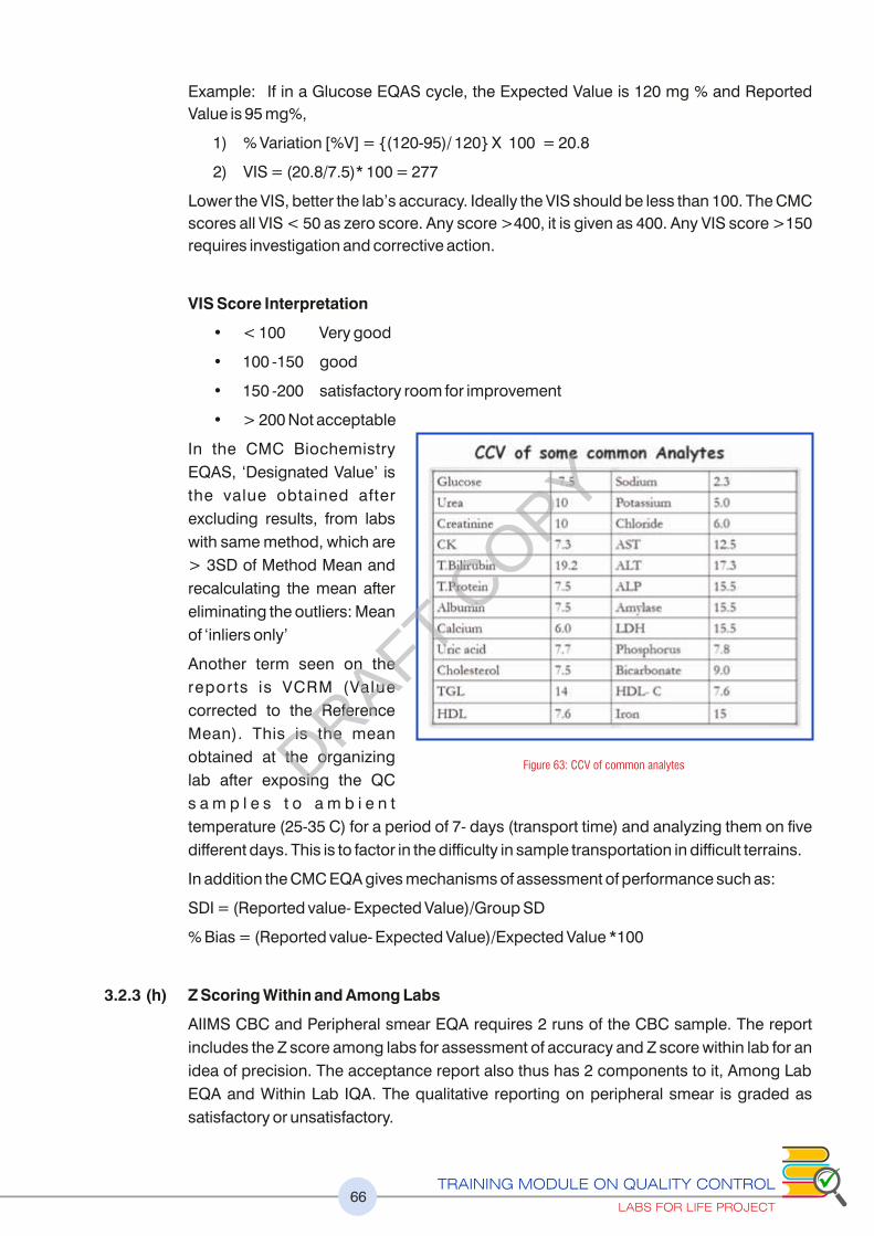
TRAINING MODULE ON QUALITY CONTROL
LABS FOR LIFE PROJECT66
Example: If in a Glucose EQAS cycle, the Expected Value is 120 mg % and Reported
Value is 95 mg%,
1) % Variation [%V] = {(120-95)/ 120} X 100 = 20.8
2) VIS = (20.8/7.5)* 100 = 277
Lower the VIS, better the lab’s accuracy. Ideally the VIS should be less than 100. The CMC
scores all VIS < 50 as zero score. Any score >400, it is given as 400. Any VIS score >150
requires investigation and corrective action.
VIS Score Interpretation
• < 100 Very good
• 100 -150 good
• 150 -200 satisfactory room for improvement
• > 200 Not acceptable
In the CMC Biochemistry
EQAS, ‘Designated Value’ is
the value obtained after
excluding results, from labs
with same method, which are
> 3SD of Method Mean and
recalculating the mean after
eliminating the outliers: Mean
of ‘inliers only’
Another term seen on the
reports is VCRM (Value
corrected to the Reference
Mean). This is the mean
obtained at the organizing
lab after exposing the QC
s a m p l e s t o a m b i e n t
temperature (25-35 C) for a period of 7- days (transport time) and analyzing them on five
different days. This is to factor in the difficulty in sample transportation in difficult terrains.
In addition the CMC EQA gives mechanisms of assessment of performance such as:
SDI = (Reported value- Expected Value)/Group SD
% Bias = (Reported value- Expected Value)/Expected Value *100
3.2.3 (h) Z Scoring Within and Among Labs
AIIMS CBC and Peripheral smear EQA requires 2 runs of the CBC sample. The report
includes the Z score among labs for assessment of accuracy and Z score within lab for an
idea of precision. The acceptance report also thus has 2 components to it, Among Lab
EQA and Within Lab IQA. The qualitative reporting on peripheral smear is graded as
satisfactory or unsatisfactory.
Figure 63: CCV of common analytesDRAFT COPY

TRAINING MODULE ON QUALITY CONTROL
LABS FOR LIFE PROJECT67
3.2.3 (i) Youden Plots
Some EQA schemes use two
control samples of different
levels in order to check the
performance of the analytical
m e t h o d i n d i f f e r e n t
concentration/activities, and
preferably close to the decision
limits. When 2 EQA samples –
high and low are analysed by
each lab either by same method
analytical principle, instrument,
r e a g e n t ( o r b y d i f f e r e n t
techniques in which case a
different plot is made), the
observed results plotted as a
Youden p lot . Th is a l lows
comparison of the relationship
of each level’s value to the group’s performance. Youden plot is a rectangular chart of
which the four angles correspond to the control limits of the two control levels [-4SD -
+4SD]. The acceptable part, the mid-zone and the rejected part have different colors.
Each dot represents a different laboratory and therefore Youden plot describes the whole
EQAS scheme. Dots (laboratories) that lie across the diagonal of the rectangular, at 45o
(The Manhattan Mean or MM), but are far from the center correspond to laboratories with
proportional analytical error. The greater the distance from the center, the greater the
proportional error. Dots restricted in the central rectangular, correspond to laboratories of
which the performance is considered acceptable for this specific analyte. The service
providers mark your lab among the dots.
In India, The CMC Hemostasis EQAS adopts this scheme in addition to the bar graphs.
Both peer and method comparisons are made and the acceptability reported as within/
Out-with consensus.
3.3 Qualitative and Semi-Quantitative EQA in India
Qualitative assessment of tests are done for staining, culture and serology in microbiology,
cytology, histopathology, IHC, Peripheral smears in pathology, blood grouping, cross
matching, Coomb’s testing and TTIs in blood banking are available with many service
providers.
Please see the annexure no 5 for the frequency and Scope of Testing of Commonly
used EQA Schemes in India
3.4 Inter Laboratory Comparison (ILC) Programs (Peer Group Comparisons)
Several IQC providers, make available ILC data. These are robust checkpoints for the
evaluation of accuracy of the lab tests. For several reasons, the peer group comparison data
may be considered as the most robust version of ILC/EQA.
Figure 64: Youden Plot
DRAFT COPY

TRAINING MODULE ON QUALITY CONTROL
LABS FOR LIFE PROJECT68
The ILC peer groups are created by the service provider of the lab’s Internal Quality
Controls and thus is it is very important to build the peer group data availability into the
IQC purchase. The service providers creates groups for the same method and equipment
as well as that for all labs reporting on that analyte; often termed group values, on an
ongoing basis. The labs feed their data into the centralized base. The lab’s results may
then be compared with the peer group for both accuracy and precision and the reports
made available periodically.
• Your laboratory enrolls in an inter-laboratory program offered by your QC
manufacturer.
• Your laboratory, along with other laboratories, analyze the same lot number of
control materials for the month.
• Your laboratory submits your QC results through a QC data management
program to a central facility.
• The central facility examines the data for outliers and calculates the means and
SDs for the peer group and all-lab group, and SDI and CVI for your laboratory.
• Your laboratory receives a report indicating your analytical performance.
Consensus Based Metrics such as SDI for accuracy and CVI for comparison of your lab’s
precision to the other participant labs is also provided. SDI has been discussed in the
earlier section. CVI is the Coefficient of Variation Index and is calculated by dividing the
lab’s monthly CV by the CV of all the values. Ideally, CVI ��1.0, since your values are from
a single lab, while the peer CV is from several laboratories. The smaller the number, higher
the precision in your lab.
If CVI = 1.5 to 2.0, your lab is 50-100% less precise than its peer group, usually
requiring investigation.
As in the Proficiency Testing Comparators, the ILC groups can be your peer using the
same method and equipment (blue arrow) or that of the all-labs group (red arrow). Also
monthly as well as cumulative data is made available. (Figure 66)
Figure 65 : Diagrammatic representation of collecting, compiling, analysis and dissemination of peer group data
DRAFT COPY

TRAINING MODULE ON QUALITY CONTROL
LABS FOR LIFE PROJECT69
The figure 67 below shows an ILC report for Direct Bilirubin by diazotization method (red
horizontal circle), done on Beckman Coulter Equipment AU 400 to 5800 (red horizontal
circle), by 153 labs collecting 22,609 data points (L1 & L2, Cumulative). Level 1 and 2
controls (Red and Green vertical circles) are used. Monthly and cumulative data (Red and
Green dotted arrows) are collected and computed. Mean, SD CV, number of data points
and number of labs are shown in the report.
Such a robust mean allows anchoring as the true/ target value for any kind of comparison
and calculation. Please also refer to the advantages of having such a target value in the
IQC monitoring, enabling the calculation of TE, SEc and Sigma-metrics.
ISO also allows this kind of comparison as an alternative approach albeit in the absence
of formal EQA/ILC programs. 5.6.3. 2 last sub clause.
3.5 Split Testing (Exchange of Samples)
For those tests where no formal PT program is available, ISO recommends “exchange of
samples with other laboratories” as an alternate method. 5.6.3.2. What is implied here is that
the lab send a sample to one or more reliable/accredited labs and compare the results. Using
a minimum of 2 comparison labs is recommended. Clinical Pathology samples like Urine,
Figure 66: Kinds of peer group comparisons made available in a peer group reports
Figure 67: Example of peer group comparison data, specific for equipment and method, for 2 levels of QCs with monthly and cumulative statistics and the number of participating labs and data points
DRAFT COPY

TRAINING MODULE ON QUALITY CONTROL
LABS FOR LIFE PROJECT70
Stool, and Cavity Fluids are generally analyzed for proficiency in this way. Some high end
tests such as Bone Marrow, IHCs, molecular biology and cytogenetics are also subjected to
proficiency testing thus. Some of these are available in the international EQAS and must be
ideally registered with those providers.
Some labs also do inter-observer variance as a substitute to exchanging samples with other
laboratories. For unstable analytes like semen analysis where time lapse affects the motility,
such measures may be acceptable. Decisions on these may be taken and documented by
the lab in alignment with the requirement of any accreditation bodies.
Periodicity of testing, acceptance criteria, authority for review of acceptance should be
defined for each analyte and documented.
3.6 Troubleshooting and Corrective Actions
The following are points to be noted and about wrong PT/EQA reports
Spurious errors should be avoided. As EQAS is appraising the analytical part of the testing,
all effort should be directed at avoiding careless mistakes which will result in meaningless
EQAS reports
1. Incorrect classification of testing methods leading the service provider to analyze the
lab’s report with the wrong peer
2. Incorrect units / conversion leading the service provider classify the reports as incorrect
3. Incorrect sample tested. If there is a serial number / lot number in the lyophilized
testing material caution must be exercised in identifying the sample correctly
4. Technical errors – reconstitution/dilution inadequate mixing. Have a separate calibrated
pipette to do the reconstitution of EQAS samples. A fixed volume pipette will be appropriate.
5. Transcription errors
Please refer annexure 6B for EQA (PT failure checklist) corrective action format
Actual Analytical Errors should immediately lead to serious investigations and root
cause analysis.
a. Relook at the IQC data
b. Are there trends? High/low bias?
c. Change in reagents?
d. Changes in calibrators?
e. Look for acceptance testing details, lot verifications.
f. Storage of reagents, Calibrators?
g. Change in the environment?
h. Water quality?
I Operator?
j. Investigate Equipment performance: aspiration system, incubators, cuvette systems,
optical system, refrigeration system
DRAFT COPY

71
METHOD EVALUATION
PART 2
AS PER ISO: 15189 5.3.1.2 AND 5.5.1
DRAFT COPY
TRAINING MODULE ON QUALITY CONTROL
LABS FOR LIFE PROJECT72
Learning Objectives
At the end of this chapter, the learners will be able to understand the
Difference between validation and verification
Pre-purchase assessment of equipment using statistical tools
Setting up of acceptance testing program for newly procured equipment
CHAPTER 4: METHOD EVALUATION
“4.1 Validation and Verification
Many a times the terms are used interchangeably. However, they are not the same.
Validation is “the process of testing a measurement procedure to assess its performance
and determine whether that performance is acceptable” and is typically a manufacturer’s
activity. Verification is simply verifying the manufacturer’s claims for performance
specifications. It is typically performed in a clinical laboratory for implementing an FDA-
approved instrument/method. It is a much simpler and streamlined method than validation.
ISO 15189: 2012, in clause 5.3.1.2 mandates equipment acceptance testing. Performance
specifications as claimed by the manufacturer is derived under ideal conditions. The
working condition of the lab may not be able to replicate that ideal condition. Besides, the
transportation of the equipment can affect the factory settings. Thus it is incumbent on the
laboratory that upon installation, the equipment is verified and the claims of the
manufacturer reestablished.
As per 5.5.1 it is also incumbent upon the laboratory to use validated examination
procedures. These procedures are also to be subjected to independent verification in the lab
by obtaining objective evidence in the form of performance characteristics, to establish the
claims put forward by the manufacturer.
Acceptance testing may further be modified into performance evaluation for fitness of
purpose, by using sigma metrics.
This section explains the process of this verification and performance evaluation. In addition,
the section explains a method for assessing the “fitness for purpose” of the equipment prior
to purchase, by calculating the sigma metrics, using the manufacturer supplied
performance data. An FDA approved method just means that the claimed performance
specifications have been verified. It does not necessarily mean that the method performance
will be acceptable for the purpose for which it is intended. The onus is on the lab to
understand this and pre-verify the suitability of the method.
DRAFT COPY
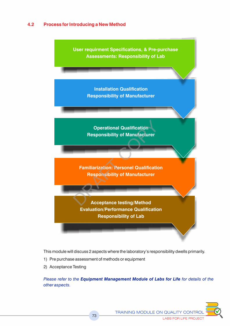
4.2 Process for Introducing a New Method
This module will discuss 2 aspects where the laboratory’s responsibility dwells primarily.
1) Pre purchase assessment of methods or equipment
2) Acceptance Testing
Please refer to the Equipment Management Module of Labs for Life for details of the
other aspects.
TRAINING MODULE ON QUALITY CONTROL
LABS FOR LIFE PROJECT73
Acceptance testing/Method
Evaluation/Performance Qualification
Responsibility of Lab
Familiarization: Personel Qualification
Responsibility of Manufacturer
Operational Qualification
Responsibility of Manufacturer
Installation Qualification
Responsibility of Manufacturer
User requirment Specifications, & Pre-purchase
Assessments: Responsibility of Lab
DRAFT COPY

4.3 Pre-purchase Assessment
When a lab decides to introduce a new test or procure equipment, several factors are considered. An
URS or User Requirement Specifications based on the lab’s requirement in terms of quality
specifications, robustness of the method, cost implications and in the case of an equipment, its
throughput, and accessories required, service and spare-part availability, environmental
requirements are considered among several others. Based on the URS, the lab may evaluate
several brands available in the market. The lab is generally given the product details in the form
of product inserts. These inserts will specify the Performance Characteristics. In the case of FDA
approved methods, it ensures that these specifications have been verified by the authorities
concerned. But what it does not guarantee is the suitability of the method for the intended use.
The lab is well advised thus to evaluate the fitness for purpose through evaluation of total error
and sigma metrics of the method at all clinical decision levels. This may be done using the 4 key
numbers, the CVs or SDs specified by manufacturer, bias values derived from the Slope and the
intercept (also supplied by the manufacturer) and TE (from any source like BV).A
Let us consider two examples, calcium and glucose, from certain product inserts
TRAINING MODULE ON QUALITY CONTROL
LABS FOR LIFE PROJECT74
Figure 68: Pre-purchase verification using manufacturer’s kit insert (An example)
Figure 69: Pre-purchase verification using manufacturer’s kit insert (example 2)
DRAFT COPY
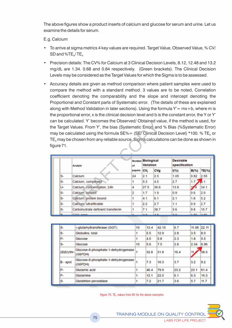
TRAINING MODULE ON QUALITY CONTROL
LABS FOR LIFE PROJECT75
The above figures show a product inserts of calcium and glucose for serum and urine. Let us
examine the details for serum.
E.g. Calcium
• To arrive at sigma metrics 4 key values are required. Target Value, Observed Value, % CV/
SD and %TE / TEA A
• Precision details: The CV% for Calcium at 3 Clinical Decision Levels, 8.12, 12.48 and 13.2
mg/dL are 1.34. 0.68 and 0.84 respectively. (Green brackets). The Clinical Decision
Levels may be considered as the Target Values for which the Sigma is to be assessed.
• Accuracy details are given as method comparison where patient samples were used to
compare the method with a standard method. 3 values are to be noted, Correlation
coefficient denoting the comparability and the slope and intercept denoting the
Proportional and Constant parts of Systematic error. (The details of these are explained
along with Method Validation in later sections). Using the formula Y’= mx+b, where m is
the proportional error, x is the clinical decision level and b is the constant error, the Y or Y’
can be calculated. Y’ becomes the Observed/ Obtained value, if the method is used, for
the Target Values. From Y’, the bias (Systematic Error) and % Bias (%Systematic Error)
may be calculated using the formula SE%= (SE/ Clinical Decision Level) *100. % TE or A
TE may be chosen from any reliable source. Sigma calculations can be done as shown in A
figure 71.
Figure 70: TE values from BV for the above examples A
DRAFT COPY
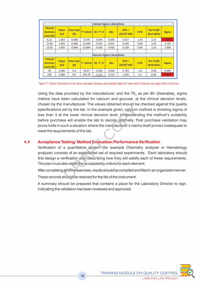
TRAINING MODULE ON QUALITY CONTROL
LABS FOR LIFE PROJECT76
Figure 71: Sigma Calculation for the above examples showing unacceptable Sigma for lower limit of Calcium and upper limits of Glucose
Using the data provided by the manufacturer, and the TE as per BV (Desirable), sigma A
metrics have been calculated for calcium and glucose, at the clinical decision levels,
chosen by the manufacturer. The values obtained should be checked against the quality
specifications set by the lab. In the example given, calcium method is showing sigma of
less than 3 at the lower clinical decision level. Understanding the method’s suitability
before purchase will enable the lab to decide optimally. Post purchase validation may
prove futile in such a situation where the manufacturer’s claims itself proves inadequate to
meet the requirements of the lab.
4.4 Acceptance Testing/ Method Evaluation/Performance Verification
Verification of a quantitative system (for example Chemistry analyzer or Hematology
analyzer) consists of an established set of required experiments. Each laboratory should
first design a verification plan describing how they will satisfy each of these requirements.
The plan must also detail the acceptability criteria for each element.
After completing all of the exercises, results should be compiled and filed in an organized manner.
These records should be retained for the life of the instrument.
A summary should be prepared that contains a place for the Laboratory Director to sign,
indicating the validation has been reviewed and approved.
DRAFT COPY

TRAINING MODULE ON QUALITY CONTROL
LABS FOR LIFE PROJECT77
4.5 Verification Plan
4.6 Understanding Quality Requirements
The lab has to define its quality requirements to ensure that the test selected meets intended use for
that test. It is the laboratories’ responsibility to the define the quality required and then judge the
acceptability on the basis of the performance observed in the laboratory against the goals selected.
The lab also has to verify the claims by the manufacturer for specific performance characteristics
as per quality specified by the lab. (See below as an example, where the laboratory selects the
sigma-metric of 3 as the minimum performance quality required for this selected test to meet,
before it can be judged acceptable. If the lab chooses the quality requirement as TE = Bias +3
SD, and TE is chosen from CLIA, then using the data from the exercises, the lab has to calculate A
the Total Error using that formula. Bias +3 SD should be less than the CLIA TE . Alternatively the A
lab may choose a defendable and attainable Sigma limit to refer the verification against.
Care must be exercised that the quality specifications chosen should be both attainable
and defensible.
"An illustrative example of Quality Specifications of a lab for an analyte."
TE<TEA
Meet or exceed manufacturer’s performance specifications and/or
If the lab chooses 3 SD as the quality specification and CLIA as the chosen TE , then,A
TE= Bias + 3SD < CLIA TEA
(%TE= %Bias + 3CV% < CLIA %TE )A
Sigma Metrics; A sigma of >3
or as decided by the quality requirement of the lab for the quality of that analyte
As seen in the ongoing method evaluation, it will be good to evaluate the method for
sigma scale, at all clinical decision levels.
Define Quality requirement
Select appropriate types of experiments to reveal analytical errors
Collect experimental data
Use statistical tools on the data to estimate size of anlaytical errors
Compare the observed errors with the defined allowable error
Judge the acceptablitity of observed performance characteristics
If method is acceptable, then perform rerence range experiment
Put into routine use
DRAFT COPY
TRAINING MODULE ON QUALITY CONTROL
LABS FOR LIFE PROJECT78
4.7 Select Performance Characteristics considered under method evaluation
Ideally seven performance characteristics that should be evaluated before reporting results
of a new test method/system as per CLSI guidelines include:
1. Precision
2. Accuracy (measured bias) or comparability (measured differences)
3. Linearity over the measuring interval or analytical measurement range (AMR)
4. Limit of detection (LoD) and limit of quantitation (LoQ or analytical sensitivity)
5. Specificity or interference
6. Reagent or sample (analyte) carryover
7. Reference interval or decision value (interpretive information)
In the following sections, each of these performance characteristics is explained. The
definition of the performance characteristic, collecting data for the exercise, running the
experiment, data analysis using statistical tools, evaluation of data and acceptability
criteria are explained. Finally, drawing the conclusions on method performance by
analyzing each data set, verifying it against set quality goals (TE< TEa or meeting the sigma
performance), and finally the documentation of the evaluation exercise and introduction to
routine service is explained.
4.8 Precision
Precision is the agreement of the measurements of replicate runs of the same sample.
Replication experiments are performed to estimate the imprecision or random error of the
analytical method. Precision is measured in terms of coefficient of variation (CV).
EP15: a five-day procedure to verify that imprecision meets the claims of a measurement
procedure (EP15 is most frequently used by clinical laboratories for method evaluation.)
EP05: a 20-day procedure to establish the imprecision for a measurement procedure.
4.8.1 Things to keep in mind while doing the precision exercise
• Time period: within-run, within-day, day-to-day
• Number of runs of the same sample: minimum of 20
• Sample matrix: patient sample or simulate patient sample
• Analyte concentration: medical decision limit
• Calculations: mean, standard deviation (SD), coefficient of variation (CV)
Precision will be evaluated by running between-day (intermediate precision) using normal
and abnormal control samples and within-day (repeatability) precision using patient
samples at different clinical decision levels. Between-day precision can be tested by running
each QC once per day for 20 days or 4 times a day for 5 days. Within day precision will be
tested by running each sample 20 times in one day. The mean, standard deviation (SD), and
CV of the replicates will be calculated.
Guidelines for the doing the study: Precision
4.8.2 Short -Term (Within-Run/Day)
A. Sample:
1. Two levels (Low / High or Normal / Abnormal)
2. Patient or quality control
DRAFT COPY

TRAINING MODULE ON QUALITY CONTROL
LABS FOR LIFE PROJECT79
3. Select values near the medical decision point(s) of interest for the analyte
B. Testing:
1. Ensure there is a sufficient reagent to perform all the 20 tests.
2. Run each sample 20 times on the same run, if possible, or least within the same day.
C. Acceptability criteria:
1. Calculate the coefficient of variation (CV) for each level using 20 data points.
2. Compare the calculated CV to the manufacturer’s stated precision claims found in the
package insert.
3. If manufacturer’s precision cannot be met, it is acceptable to attain precision that is
<25% of the CLIA Allowable Error or BV Imprecision of Desirable or Minimal.
4. If Short -Term precision is unacceptable, consult the instrument’s manufacturer for
technical assistance.
5. If unable to resolve issues with short-term precision, the method validation process
should be discontinued and a new method selected for potential implementation.
4.8.3 Long-Term (Between-Run/Between Day Labs for Life QC Tool: LJ with CV trends)
A. Material Used:
1. Two / Three levels (Low/High or Normal/Abnormal)
2. Control Material. A lab may already have this data available from their daily QC runs.
B. Testing: Run the QC once a for 20 days or 4 times a day for 5 days to collect minimum 20
data points
C. Acceptability criteria:
1. Calculate the CV for each level using the 20 data points
2. Compare to manufacturer’s stated precision claims found in the package insert.
3. If manufacturer’s precision cannot be met, it is acceptable to attain precision that is
<33% of the CLIA Allowable Error
4. If Long-Term precision is unacceptable, consult the instrument’s manufacturer for
technical assistance.
4.9 Accuracy [Trueness] (Measured as Bias) (“correlation studies”)
Accuracy is the true value of a substance being measured. Verification of accuracy is the
process of determining that the test system is producing true, valid results and is expressed
numerically as bias.
Estimate of bias or systematic measurement error is done by quantifying the average
difference between results from a measurement procedure and results from an accepted
reference measurement procedure. When a reference measurement procedure is not
available for an analyte, a best-available comparative method may be used to measure bias.
Frequently, clinical laboratories perform a comparison of patient sample results between a
new and an existing measurement procedure. In the instances where the comparison
method is not a reference method, then the trueness of the new method cannot be
determined. The laboratory would then be measuring the difference between the methods
DRAFT COPY

TRAINING MODULE ON QUALITY CONTROL
LABS FOR LIFE PROJECT80
and not the bias of the new method. Any difference between the test method and the
comparative method must be carefully interpreted.
CLSI Guidelines for Trueness (Measured as Bias) EP15: a method comparison to verify that a
new method conforms to a manufacturer’s claim for comparability to another procedure.
(Minimum of 20 patient samples). EP09: a method comparison to establish a claim for
method comparability. (Minimum of 40 patient samples)
4.9.1 Guidelines for the doing the study: Accuracy
a. Determine your comparison or reference method.
i. The comparison method must be previously validated.
ii. The comparison method must be currently performing successfully in EQA.
iii. The ideal comparison method is a similar instrument/method.
iv. Comparison to an in-house method is preferred if the in-house instrument meets the
above criteria.
v. Samples with known values, such as proficiency testing samples or commercial
standards, may be used as the reference method.
b. Sample Criteria
i. A minimum of 20 samples that cover the reportable range of the method and include
points near the Medical Decision Points.
ii. Patient, quality control, and proficiency testing materials may be used.
iii. 50% of the selected samples must lie outside of the current reference range.
c. Testing
i. Run each sample in duplicate on each instrument
1. Ideally, samples should be run within 2 hours of each other unless the analyte
has a shorter stability.
2. Analyze the replicates (duplicates) in different runs and in a different order.
ii. Retain the instrument print-outs.
iii. Duplicates should be averaged.
iv. Data should be plotted immediately to identify and correct any outliers by reviewing
the Comparison Plot or Difference Plot Labs for Life QC Tool: Accuracy the
Westgard website under Paired Data Calculator.
• Re-analyze any discrepant results between the test and comparative methods to
confirm that the differences are real and not mistakes in recording the values or
mix-ups of specimens.
• If an outlier is identified, then investigate the reason and take corrective action.
• Document the findings.
• Remove the outlier from the data set.
d. Time Period of Testing
i. A minimum of 5 separate days must be used for testing.
ii. This experiment can be performed simultaneously with the long-term precision study.
DRAFT COPY

TRAINING MODULE ON QUALITY CONTROL
LABS FOR LIFE PROJECT81
e. Evaluation of Data
i. Calculate the slope, Y-intercept, Sy/x, and r. (Explained later)
ii. Evaluate the data.
4.9.2 Checking Correlation and Quantifying Error through Linear Regression
Where accuracy is concerned, 2 major factors should be considered. The degree of
agreement or correlation between 2 sets of data and the biases involved despite good
correlation. The degree of correlation is expressed as correlation coefficient or r. In earlier
discussions we have seen that biases in a measurement system are quantified as Systematic
Errors (SE). The Systematic errors can be of two types, Constant Error and Proportional
Error. In addition, the data includes Random errors (Imprecision)
Linear regression yields all these 4 kinds of data. (In the example below, 3 of these are
illustrated). The reference method (red line) and test data (blue line). The yellow table on the
left shows the raw data used. (Exaggerated numbers are used to clarify the concept. In real
measurements, the differences will be subtle and close observations are required.).
Linear regression consists of finding the best-fitting straight line through the data points of
the 2 sets of data.
1. r. When 2 sets of data are plotted on a graph with the reference method as the X axis and
test method as the Y axis, best-fitting line through these points is called a regression line.
r is a statistical measure of the degree of agreement between 2 sets of data about how close
the data are to the fitted regression line. This can be a helpful tool in determining the strength
of the relationship between two variables as we can predict scores of one variable from the
scores of the second variable. This valuable numerical measure of association between two
variables, the Pearson’s or correlation coefficient or r, has a value between -1 and 1
indicating the strength of the association of the observed data for the two variables.
• 0 says no relationship exists
• 0 ��1 explains there is a correlation which is directly proportional
• 0 ��explains that there is a correlation which is inversely proportional
• 1 indicates that the model explains all the variability of the response data
around its mean.
• For a method to be comparable, the r must be > 0.975
2. Intercept: When 2 sets of data are plotted on a graph with the reference method as the X
axis and test method as the Y axis, there could be a constant difference between these 2
sets regardless of the concentrations involved. This is called constant error. In the
example below, each of the test value is 20 points more than reference. Such differences
are generally seen as in the case of interfering substances. For the calculation of
systematic errors, the formula Y/Y' = mX+b is used where b is the constant error.
3. Slope: When 2 sets of data are plotted on a graph with the reference method as the X axis
and test method as the Y axis, there could be errors which are proportional to the values.
These are called proportional errors. In the example below, the test is 40% more than the
reference value. For the calculation of systematic errors, the formula Y/Y' = mX+b is used
where m is the proportional error
DRAFT COPY

TRAINING MODULE ON QUALITY CONTROL
LABS FOR LIFE PROJECT82
Both constant and proportional errors contribute towards Systematic Errors (Bias)
4. Sy/x is the random error component in the calculation of the paired data. This
component is not used in method evaluation. The random error from intermediate precision
study is used for method evaluation. Sy/x is not further discussed in this module
4.9.3 Assessing Acceptability criteria:
Linear regression analysis will be used to determine if the methods are accurate within the
specified TEa when the Correlation Coefficient (r) is >0.975. If the Correlation Coefficient/ “r” is
< 0.975, then more patient data must be collected. If the Correlation Coefficient remains <
0.975, then paired data calculations or another regression analysis technique needs to be used.
The following process may be adopted for evaluation.
Regression Plots Interpretations
Constant Error: Intercept
There is a constant difference of 20 between the reference and test.
The Y’ has a constant error of 20. This value is called the intercept or
the b in the equation;
Y’= mx+b. On the graph, please note the shifting of the blue line away
from 0. The constant errors are generally due to interferents. As there
is no proportional error, there is no m value in this case. The formula
requires addition of b to the X to derive Y’.
r = 1 denoting good correlation, regardless of the steep Constant
Error. Proceed to Sigma Metrics.
Proportional Error: Slope
The test is 40% more than the reference value. The error is
proportional all levels and thus the m of the Y’= mx+b. The formula
requires multiplication of the value of x by 1.4 to get the predicted Y.
The blue and red lines start from 0 but the gap widens as the values
increase.
There is no b value in this case as there is no constant error
r is 1 denoting good correlation despite the proportional error. .
Proceed to Sigma Metrics.
In this graph there is both constant and proportional errors which are
quantified by the formula mx+b. These numbers can be used for any
predictions of Y. As the r = 0.998, the method is comparable and the
predictions are valid. The formula requires multiplication of X by m
(0.97) and addition of b (2.83). Proceed to sigma metrics
Here the r is 0.751. The fact is evident from the visual assessments as
these are exaggerated numbers. However, for numbers with smaller
differences, the r should be monitored before error calculations are
assessed. Any value< 0.975% shows lack of correlation and
requires repeat process with more samples.
Figure 72: Explanations for regression plots with illustrative examples
DRAFT COPY
TRAINING MODULE ON QUALITY CONTROL
LABS FOR LIFE PROJECT83
4.9.3 (a) Visual Assessment of Linear Regression graph
Visually inspect the comparison plot for linearity and outliers. Remove outliers. If an outlier
is removed, then recalculate the regression statistics. If the regression graph and r are
acceptable, proceed as follows.
4.9.3 (b) Determine Bias or Difference between the Methods
Define Medical Decision Points. A Medical Decision Point (MDP) (see below) is the
concentration of the analyte at which a medical decision is triggered and/or laboratory
established critical values.
1. Using the linear regression equation, calculate the predicted Y/Y' value that
corresponds to the concentration of MDP
2. Determine the bias (difference) by subtracting MDP from Y’
3. Calculate the % bias (% difference) as bias/MDP * 100.
4.9.3 (c) Calculate Sigma- metrics.
Using the SD/CV% from the precision experiment, TE / TE %, MDPs (See Below) as A A
targets, Bias/ % Bias from the above accuracy experiment, calculate the sigma
performance of the new method at each clinical decision point using the formula,
Sigma = (TE - Bias)/SD or (TE %- Bias %) / CV%. Judge acceptability. as per defined A A
quality specifications of the lab (See below).
The lab should define in its quality specifications about acceptable performance.
In addition to Sigma-Metrics or instead of Sigma Metrics, the lab can opt for comparisons
of TE with TE as followsA
4.9.3 (d) Check TE against TE : A
TE< TE Using the formula TE= Bias+ n* SD or Bias % + n* SD or Bias% + n* CV%. The A
chosen n is the lab's prerogative. An n of 3 is suggested.
TE= Bias + n* SD < CLIA TEA
OR
(%TE= %Bias + n* CV% < CLIA %TE )A
RECAP
TE<TEA
Meet or exceed manufacturer’s performance specifications and/or
TE= Bias + n* SD < CLIA TEA
(%TE= %Bias + n* CV% < CLIA %TE )A
And / Or
Sigma Metrics; A sigma of >3
(or as decided by the quality requirement of the lab)
As seen in the ongoing method evaluation, it will be good to evaluate the method for
sigma scale, at all clinical decision levels.
Figure 73: Clinical Decision Levels; An excerpt
DRAFT COPY

TRAINING MODULE ON QUALITY CONTROL
LABS FOR LIFE PROJECT84
4.9.3 (e) Medical Decision Point/Clinical Decision Point:
Are those concentrations of the anlayte that makes an impact in clinical decisions. While
evaluating methods it is important to check the accuracy at each of these points.
To read more, please check https://www.westgard.com/decision.htm
(Please refer annexure number 3: Medical Decision Points)
Recap of Evaluation Process
For example, if the method being validated is calcium,
• Computations should be done using 7,11 and 13.5 mg/dL as the target X,
• Using the m and b values from the regression analysis calculate the Y’
• Find the bias/ bias%
• Get the corresponding SD/CV%
• Define the quality requirement (TE / TE %)A A
• Calculate the sigma at each level
4.9.3 (f) Blandt Altman Plot
In a Blandt Altman plot, in addition to the regression, a difference plot and even a percent
difference plot is done. The concept of Blandt Altman is explained below. This can also be
easily done using scatter plots on the Excel.
Regression Plots Interpretations
A set of 7 data points are given in the chart as an
example. A minimum of 20 data sets are required for
this exercise. The mean of the 2 values, difference or
Bias (Test- Reference), % Difference or Bias
(Bias/Reference*100) are calculated.
The values range covering the range of performance
expected, in this case, from 10-1090
The data is used to obtain the linear regression.
Shows an acceptable correlation of 0.99. Note the
m and b values of 0.9647 and -1.013 respectively.
The data chart also shows a negative bias
(negative b value) for the new method being
assessed
On this plot, both the difference (blue diamonds)
and the % Difference (red squares) are plotted. The
values are scattered on both sides of 0 (red arrow).
However, a negative bias is noticed, with more data
points on the negative side. The bias looks
exaggerated in the case of difference in units and
less pronounced in % difference plot. The
difference plots give a quick assessment of the
performance visually.
DRAFT COPY

TRAINING MODULE ON QUALITY CONTROL
LABS FOR LIFE PROJECT85
Another set of data points where the Test values show
a considerable positive bias
The R value is still acceptable, but notice the b
value has gone up considerably which will affect
TE calculations that could push TE>TEa or give a
low sigma value
The difference and % difference plots show all
values on the upper side of Zero (red arrow).
Difference (blue diamonds) and the % Difference
(red squares) are all above zero. At the lower
concentration of analytes, however the %bias is
more pronounced between 20-40%. At higher
concentrations, the %bias is less, between 10 and
20%. That the % Bias is more conclusive is evident
from the plot. At lower levels, the unit bias is small,
but the % Bias is significant. In the case of higher
values, this is just the opposite
Figure 74: Illustrative example with explanation for Blandt Altman
Blandt Altman plots thus give bias and % bias plots in addition to the linear regression
data and valuable details for visual assessment. The lab is now required to assess the
data elicited against its quality specifications. Visually scan for significant and dramatic
differences at the upper and lower ends of the range. Positive or negative biases should
be addressed by repeating the accuracy exercise. In the event of persistent biases, a
reevaluation biological reference range must be done
4.10 Linearity
Linearity studies are performed to determine the linear reportable range for an analyte. The
linearity for each analyte is assessed by checking the performance of recovery throughout
the manufacturer’s stated range of the testing system. This is done using a set of standards
containing varying levels of an analyte in high enough and low enough concentrations so as
to span the entire range of the test system. Therefore, the demonstration of the linear range
requires a series of known concentrations or known relationships established by dilution. A
quantitative analytical method is said to be linear when measured results from a series of
sample solutions are directly proportional to the concentration or activity in the test
DRAFT COPY
specimens. This means that a straight line can be used to characterize the relationship
between measured results and the concentrations or activity levels of an analyte for a
determined range of analyte values.
Linearities are performed whenever a new analyzer, analyte, or method is introduced into the
laboratory, or when an analyzer is replaced. Linearities may also be performed for
troubleshooting purposes when quality control is unacceptable and deviations from
acceptable data cannot be explained, when major analyzer repair or replacement of
components has taken place, or at intervals prescribed by the manufacturer in the
instrument’s user manual.
i. The Analytical Measurement Range (AMR) is the range of analyte values that a
method can directly measure on the specimen without any dilution, concentration, or
other pretreatment not part of the usual assay process. AMR validation is the process
of confirming that the assay system will correctly recover the concentration or activity
of the analyte over the AMR. The manufacturer defines the AMR – but it is the
laboratory’s responsibility to verify it.
ii. The Clinical Reportable Range / Reportable Range (CRR) is the range of analyte
values that a method can report as a quantitative result, allowing for specimen
dilution, concentration or other pretreatment used to extend the AMR. The laboratory
must specify the maximum concentration or dilution that may be performed to obtain
a reportable numeric result.
A linearity study is used to establish or verify the measuring interval for a measurement
method. Measuring Interval: the interval between lower and upper numerical values for
which a method can produce quantitative results suitable for the intended clinical use.
The measuring interval is verified by demonstrating a linear relationship between the
measured and expected concentration relationships.
CLSI Guideline for Linearity – Measuring Interval EP06: procedures to verify or establish
the linear measuring interval of a measurement procedure. An extended procedure is
explained here to calculate the acceptability at each level, by calculating the sigma-
metrics using the slope and the intercept derived from the linearity plot.
4.10.1 Sample Criteria
1) A minimum of 5 samples that cover the reportable range of the method.
2) When plotted, the values should ideally be equidistant from each other.
3) Quality control, commercial linearity standards, and calibrators (if a different lot number is
used to calibrate the instrument) may be used.
4) Patient specimens may be used if a high value near the expected upper range can
be found.
5) Sufficient volume of each sample must be available to analyze in triplicate and for
possible troubleshooting.
TRAINING MODULE ON QUALITY CONTROL
LABS FOR LIFE PROJECT86
DRAFT COPY

TRAINING MODULE ON QUALITY CONTROL
LABS FOR LIFE PROJECT87
4.10.2 Sample Preparation
1) If using purchased materials, refer to
manufacturer’s instructions.
2) If using patient specimens, then
perform the dilutions using the
manufacturer’s recommendation of
the diluent to use with out-of-range
specimens.
3) Select a patient specimen near the
detection limit and another patient
specimen near or slightly above the
expected upper limit of the working
range. Ensure that both specimens meet storage and stability requirements as stated by
the manufacturer.
4) Prepare 5 pools for testing as follows:
i. Label the low specimen Pool 1 and the high specimen Pool 5.
ii. Prepare Pool 2 (75/25) with 3 parts Pool 1 + 1 part Pool 5.
iii. Prepare Pool 3 (50/50) with 2 parts Pool 1 + 2 parts Pool 5.
iv. Prepare Pool 4 (25/75) with 1 part Pool 1 + 3 parts Pool 5.
v. Pool 5 is the High sample
6) Care must be taken to mix each pool thoroughly, and to protect the pools from
evaporation or other deterioration.
4.10.3 Running Samples, Plotting Graphs
1) Samples will be run in triplicate.
2) The mean value for each point will be calculated.
3) If one value deviates greatly from the others due to random error, it may be removed from
the data analysis and repeated.
4) Data should be plotted immediately to identify and correct any outliers.
5) Save the instrument print-outs to be filed with the summary statistics
4.10.4 Evaluation of data:
1) Determine the Assigned Value (X) for each data point:
If standards have known values, then insert them into the Assigned Value (X) column
following the manufacturer’s instructions.
If using patient dilutions,
a) Pool 3 will be used as a true value; therefore, the mean value (Y) obtained will be the
assigned value (X). ( in yellow highlighted columns in Fig 76 depicting Red horizontal arrows
how the Pool 3 mean will be the anchor value from where other targets are assigned)
b) The remaining pools will be calculated using the known relationship between
dilutions as follows:
Figure 75: Making serial dilutions for linearity test
DRAFT COPY

TRAINING MODULE ON QUALITY CONTROL
LABS FOR LIFE PROJECT88
I. Pool 1 = mean of Pool 3 x 0 = 0 (Pool 1 must be zero or near zero, or else the actual
value must be taken into account)
II. Pool 2 = mean of Pool 3 x 0.5
III. Pool 4 = mean of Pool 3 x 1.5
IV. Pool 5 = mean of Pool 3 x 2.0
2) The values obtained are then fed and the mean calculated. ( )Blue downward arrows
3) The recovered mean values will be plotted versus the corresponding assigned values. A
best-fit straight line will be drawn to connect the points on the graph with greater emphasis
on the first three points when drawing the best-fit line. Alternatively, the scatter plot may be
used on excel or Labs for Life QC Tool: Linearity may be used. Yet another alternative to
creating a graph is to use the Linear-data Plotter located on the www.westgard.com
website.
4) The plot will be visually inspected for a linear relationship. If using a paper plot, you may
not be able to go further. The visual inspection for linearity would also suffice.
5) If using a scatter plot on Excel/ Labs for Life/ Westgard, note the Slope and Intercept
derived from the regression graph.
6) Y’ is calculated using formula Y’= mX + b. (Green Highlighted Column)
7) Ideally, the slope is equal to 1.0. Acceptable Range Guideline: 0.9-1.1
8) lf the slope is outside the acceptable range, examine the results of the highest standard
first. It is possible that the test is nonlinear at its highest value
9) Ideally, the Y-intercept is equal to zero.
10) For enzyme determinations and other assays with results in high numerical values,
the Y—intercept may be much higher with no clinical significance. (In the figure
below, the intercept is 5.6) The Y— intercept for assays with low numerical values
should be 0.0 + /— 1.0
11) The predicted Y (Y’) value will be subtracted from the associated recovered/observed
mean value (Y-Y’). (Lavender Highlights, column 1) to get the absolute difference
12) % Difference will be calculated by the formula, (% Difference = (+/- Diff / y')* 100/ Predicted
Mean)* 100. This difference is the systematic error due to non-linearity. (Blue Highlight)
13) Systematic error will be compared to 50% of the total allowable error ( TE :Yellow Highlight)A
4.10.5 Acceptability criteria:
1) Visual assessment of the best-fit line on the linearity plot must demonstrate a linear
relationship. Calculate % Limit and the result should confine to 50% of the selected quality
requirement. Example as, by dividing the CLIA % TEa by a factor of 2.
2) Calculate ± Limit by either inserting 50% of the CLIA absolute value or by multiplying the
%Limit by Y’, whichever is greater.
3) Compare that systematic error to 50% of the total allowable error. The systematic error
must be less than 50% of the total allowable error.
DRAFT COPY

TRAINING MODULE ON QUALITY CONTROL
LABS FOR LIFE PROJECT89
In the example below, a method is evaluated for linearity. Assume that the manufacturer’s
claim is 5-700. The lowest recovered value however is 6. The mean of the highest is 704.
The method is linear and acceptable at all clinical decision levels.
Figure 76: Illustrative example of a linearity test. The test is linear and the error within limits at all dilutions
Figure 77: Illustrative example of a linearity test. The test is linear in the first three dilutions. The error within limits in the first three dilutions only. The limits of linearity, in this case is less than the manufacturer’s claim.
In figure 77, the dilutions yield non-linear values at higher levels. As mentioned earlier, if
the slope is outside the acceptable range, examine the results of the highest standard
first. It is possible that the test is nonlinear at its highest value. In the above example, Pool
4 and 5 values are out of linearity. A regression graph shows unacceptable slope and
intercept values. However, a line joining the lower points and the regression plot of the
same acceptable values. Fig 77, graph on the right after removing the higher values. In
this case the validated linearity is up to 354. The higher values exceed acceptable limits in
comparing with the 50% of TE . A
DRAFT COPY

TRAINING MODULE ON QUALITY CONTROL
LABS FOR LIFE PROJECT90
4.10.6 Linearity, Analytical Measurement Range and Clinical Reportable Range
In the above example, (fig 76) the manufacturer’s claim is 5-700. The lowest recovered value
however is 6. The mean of the highest is 704. However, the AMR is only 6-700 as the upper
end of AMR cannot be more than the Manufacturer’s claim. However, the lab can report an
analyte beyond the AMR by diluting sample. This range is called the Clinical Reportable
Range/ Reportable range. CRR depends upon the lab’s decision to allow dilutions. The
dilution factors must be clearly mentioned in the SOP. For example, if a 1: 9 dilution is
performed, then the CRR in the above example is 700*10= 7000. Below and beyond this the
lab will report as <6 or >7000.
Note the following terminology and corresponding figures as per the example above:
1. Manufacturer’s Claimed AMR: 0-700
2. Linearity Range: 6-704
3. Validated AMR: 6-700
4. Clinical Reportable Range: 6-7000
4.11 LoD / LoQ Limit of Detection (LoD) & Limit of Quantification (LoQ) (sometimes
referred to as “Analytical Sensitivity”)
LoD/ Sensitivity: the lowest amount of analyte (measurand) in a sample that can be
detected with a stated probability. Sensitivity is the lowest concentration of an analyte that
can be measured. For an FDA approved, unmodified method, the manufacturer’s stated
sensitivity may be used. However, the LoD will be verified for immunoassays, therapeutic
drugs, drugs of abuse, cardiac markers, and tumor markers. LoQ: the lowest amount of
analyte (measurand) in a sample that can be quantified with acceptable precision and
bias under stated experimental conditions.
Usually, laboratories review and accept the manufacturer’s claims for LoD and LoQ. But
these characteristics can be tested by laboratories using: CLSI Guideline for LoD and LoQ
EP17: procedures for verifying or establishing the LoD and the LoQ. This module is not
explaining this concept further.
4.12 Interference / Specificity
It is an artefactual increase or decrease in the apparent quantity of an analyte due to the
presence of a substance that reacts nonspecifically with the measuring system. It is the
determination of the effect of interfering substances. Most manufacturers evaluate a large
number of substances known or suspected to be potential interferents. They report this
information in the Instructions For Use (IFU). It is not practical for most clinical laboratories
to repeat such an investigation and inspection of the manufacturer’s information is
frequently sufficient. For an FDA approved, unmodified method, the manufacturer’s
stated specificity can be used.
But these characteristics can be tested by laboratories using: CLSI Guideline for Interference
EP7: procedures for testing constant error due to interference. This module is not explaining
DRAFT COPY

TRAINING MODULE ON QUALITY CONTROL
LABS FOR LIFE PROJECT91
this concept further.
4.13 Carryover
The discrete amount of reagent or analyte carried by the measuring system from one test into
subsequent test(s), thereby erroneously affecting test results.
Periodic carryover assessment is warranted in CBC analyzers. Reagent carryover among
different measurement procedures on multichannel automated biochemistry analyzers is an
evaluation that is usually conducted by measuring system manufacturers. This
characteristic can be tested by laboratories using CLSI Guideline for Carryover (EP10:
includes an assessment of sample carryover along with other parameters). Some more
details of this is explained in 4.15, page 93. Labs for Life QC Tool: Carryover
4.14 Reference Intervals
Interpretive information for laboratory test results that is frequently provided as the central
95% interval of results for a group of well-defined reference individuals. Thus BRI (Biological
Reference Interval) is the range of test values expected for a designated population where
95% of the individuals are presumed to be healthy (or normal).
When a new analytical equipment is installed the Biological Reference Range relevant for the
target population should be determined. Laboratories can produce reference intervals in a
variety of ways, including testing procedures found in CLSI Guideline for Reference Intervals
or Decision Value C28.
Procedures for establishing a reference interval are
• Verifying the suitability of a manufacturer-proposed reference interval
• Transference from the previously used reference interval by using the slope and intercept
from the accuracy testing
• Establishing a new reference interval
As said before, the Reference Interval (or Reference Range) is the range of test values
expected for a designated population in which 95% of the individuals are presumed to be
healthy (or normal). In some analytes reference interval have been replaced by decision
limits established by international consensus. For example, cholesterol (NCEP) and HbA1c
(ADA). For such analytes there is no need establish or verify the reference intervals. For such
analytes, there is no need to establish de novo or even verify the reference intervals. Rather,
laboratories must concern themselves with the accuracy of the results they report; that is,
that cholesterol values they report are not appreciably different from the values that are
reported by a certified reference laboratory on the same samples. For such analytes, the
onus falls on manufacturers to ensure their methods are traceable and on individual
laboratories to ensure they run those methods correctly (using peer group, quality control,
proficiency testing, etc.)
In instances, if medical decision limits will be used for interpretation; ensure the method
being used has validated reference intervals traceable to certified reference material and the
accuracy of your method at those medical decision levels is maintained. You should cite the
source of the medical decision limits to be used by your organization, in your reports.
DRAFT COPY
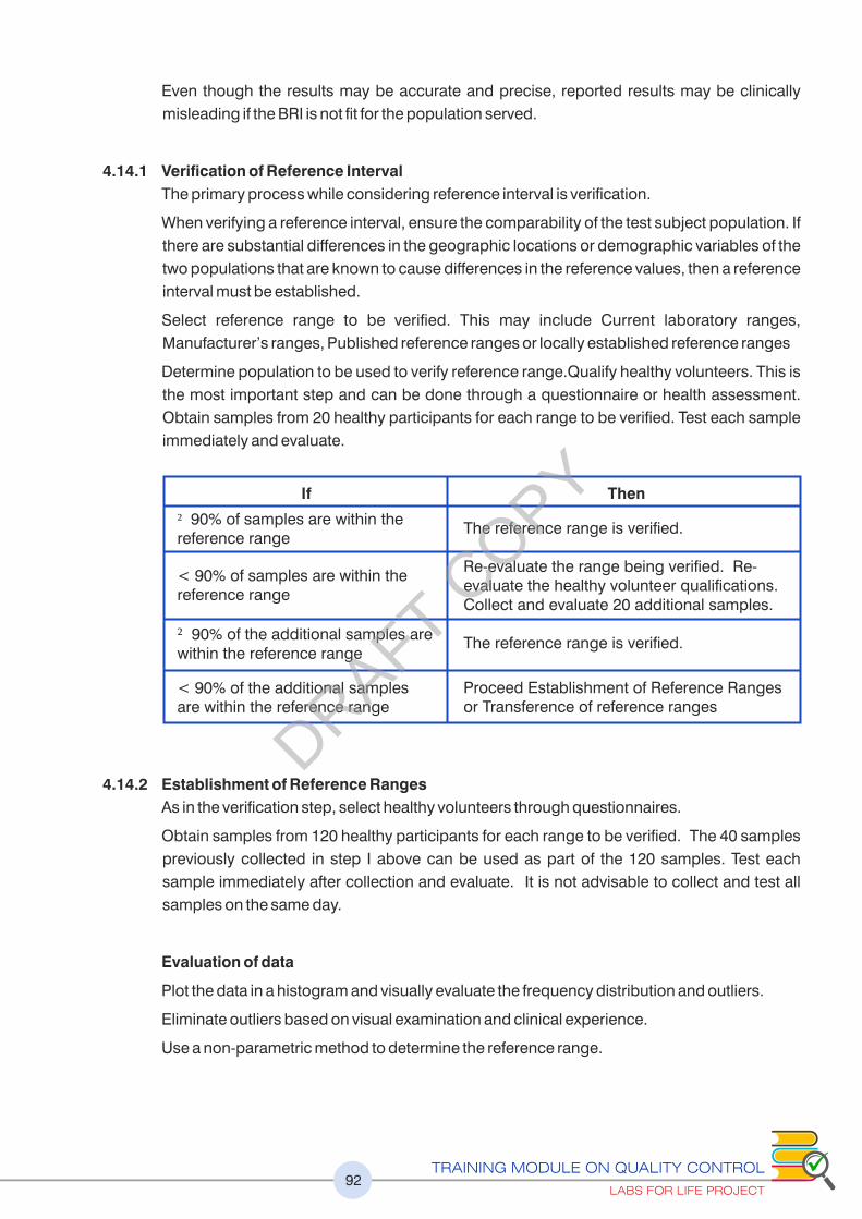
TRAINING MODULE ON QUALITY CONTROL
LABS FOR LIFE PROJECT92
Even though the results may be accurate and precise, reported results may be clinically
misleading if the BRI is not fit for the population served.
4.14.1 Verification of Reference Interval
The primary process while considering reference interval is verification.
When verifying a reference interval, ensure the comparability of the test subject population. If
there are substantial differences in the geographic locations or demographic variables of the
two populations that are known to cause differences in the reference values, then a reference
interval must be established.
Select reference range to be verified. This may include Current laboratory ranges,
Manufacturer’s ranges, Published reference ranges or locally established reference ranges
Determine population to be used to verify reference range.Qualify healthy volunteers. This is
the most important step and can be done through a questionnaire or health assessment.
Obtain samples from 20 healthy participants for each range to be verified. Test each sample
immediately and evaluate.
4.14.2 Establishment of Reference Ranges
As in the verification step, select healthy volunteers through questionnaires.
Obtain samples from 120 healthy participants for each range to be verified. The 40 samples
previously collected in step I above can be used as part of the 120 samples. Test each
sample immediately after collection and evaluate. It is not advisable to collect and test all
samples on the same day.
Evaluation of data
Plot the data in a histogram and visually evaluate the frequency distribution and outliers.
Eliminate outliers based on visual examination and clinical experience.
Use a non-parametric method to determine the reference range.
If
�90% of samples are within the reference range
< 90% of samples are within the reference range
�90% of the additional samples are within the reference range
< 90% of the additional samples are within the reference range
Then
The reference range is verified.
Re-evaluate the range being verified. Re-evaluate the healthy volunteer qualifications. Collect and evaluate 20 additional samples.
The reference range is verified.
Proceed Establishment of Reference Ranges or Transference of reference ranges
DRAFT COPY

TRAINING MODULE ON QUALITY CONTROL
LABS FOR LIFE PROJECT93
Rank (order by size) the values from lowest to highest. Example:
Multiply the total number of samples +1 by 0.025 to determine the sample number that
represents the low end of the range.
Example: Total number of samples= 120.
Low end = (120 + 1) x 0.025 = 3.025 = 3.
Sample 3 is the low end: 8.9 mg/dL.
Multiply the total number of samples +1 by 0.975 to determine the sample number that
represents the high end of the range.
Example: Total number of samples= 120.
High end = (120 + 1) x 0.975 = 117.975 = 118.
Sample 118 is the high end: 10.2 mg/dL
Use these rank values to estimate the upper and lower reference limits.
Example: Reference range is “Sample 3 to Sample 118” or 8.9 - 10.2 mg/dL
Since the assumption is that 95% of the population is healthy, removing 2.5% from the upper
and lower ends enables you to include the 95% group.
4.14.3 Transference of Reference Ranges without Verification
Labs for Life QC Tool: Reference Range by Transference
The CLSI C28-A2 describes different ways for a laboratory to validate the “transference” of
established reference intervals. Pediatric reference intervals often require this approach
because of the difficulty in obtaining sufficient specimens to establish or verify reference
intervals. If a laboratory wishes to transfer a reference interval established by another laboratory
or publication, the acceptability should be assessed based on several factors: similarity of
geographies and demographics, similarity of test methodology, sound clinical judgment and
consultation with local medical professionals. Approval by the laboratory medical director is
required and must be documented. Using the slope and intercept obtained from the accuracy
experiment, and the Lower and Upper Reference range from the previously validated method,
using the Y= mx+b equation, the new upper and lower ranges may be derived.
The BRI for the new method will be 14.5 to 51.0 by transference method. However, it is not
advised to do it more than once that is, for one change with reference to one previous method.
Female Calcium Results (mg/dL)(Data from samples 6 - 115 omitted for example purposes)
Sample 1 8.8 Sample 116 10.1
Sample 2 8.9 Sample 117 10.1
Sample 3 8.9 Sample 118 10.2
Sample 4 8.10 Sample 119 10.3
Sample 5 8.11 Sample 120 10.4
12 =(12*0.97)+2.83 = 14.5
50 =(50*0.97)+2.83 = 51.0
If slope is 0.97 and Intercept is 2.83, the current reference range is 12-50, then the new range is;
DRAFT COPY

TRAINING MODULE ON QUALITY CONTROL
LABS FOR LIFE PROJECT94
4.14.4 Prothrombin Time; Defining the mean and reference range Labs for Life QC Tool:
Coagulation
2 numbers are very important in the standardization of PT results. ISI and INR. This is
because the thromboplastin reagent used for PT estimation is very variable in its strength. PT
is a test that needs continuity. A patient on anticoagulants will need repeated estimations of
PT. So the variability within the same lab and between labs has to be minimized.
An ideal Thromboplastin will be the same as the standard PT reagent established by WHO.
Since in real practice this is not possible 2 corrective steps are undertaken.
1. Each Thromboplastin is required to be calibrated against standard PT reagent
established by the WHO and this value is called the ISI or International Sensitivity Index.
ISI value has to be assigned by the manufacturer for each lot of reagent. The lower the ISI
the more sensitive the reagent. ISI of 1.8 to 2.4 = Low sensitivity, ISI of 1.4 to 1.8 =
Average sensitivity, ISI 1.0 to 1.4 = High Sensitivity. Always look and understand the ISI
value whenever you get a new lot of PT reagent.
2. INR or International Normalized Ratio: Every lot of thromboplastin is also required to have
a population mean from the normal population. For this an estimation of MNPT or Mean
Normal Prothrombin Time is required. A laboratory can estimate the MNPT from a
minimum of 20 healthy individuals with a relatively equal mix of both sexes over a range of
age groups. (Avoid people on anticoagulants, pregnant women, and people with known
bleeding tendencies). Estimation of a geometric mean is to be preferred to the arithmetic
mean. MNPT samples must be fresh. The mean of a laboratory normal control is not an
acceptable substitute for the MNPT, since control samples may differ excessively from each
other, particularly in the case of less responsive reagents. The MNPT should be determined
with each new lot of PT reagent.
Once the MNPT is known, INR can be calculated by this formula
INR= (Patients Value/ MNPT Value) ̂ ISI
Using MNPT data to define Biological Reference Range. The reference interval is calculated
by determining the 95% Confidence interval of a group of normal donors. Ideally a number
closer to 120 is required. However, the same group that was used for MNPT will serve as the
pool for determination of reference interval.
a) Look at the individual PT result
b) Calculate mean and +/- 2 SD range
c) Exclude all those outside 2 SD
d) Now recalculate Mean +/-2 SD
e) This is the ref interval.
f) This reference interval is used in the reports
g) For good thromboplastins the reference interval falls between 10-13 secs
4.15 Carryover: Labs for Life QC Tool: Carryover Carryover is the effect of a previous sample on the next sample. Carryovers interfere with the
results. It is very important to estimate the amount of carryover. Of any test. This is particularly
DRAFT COPY

TRAINING MODULE ON QUALITY CONTROL
LABS FOR LIFE PROJECT95
important in CBC Analyzers.
Carryover % estimation in a CBC analyzer
Run any sample with high values 3 times consecutively followed by any sample with low
values 3 times consecutively and using the formula given below calculate the carryover%.
[(L1-L3) / (H1-H3)] *100
Alternatively any sample 2 times followed by 3 runs of cell pack and apply the following formula
[(Blank 1- Blank 3) /Sample 2]*100
Maximum allowable carryover % is WBC <2%, RBC < 1%, HB <2%, and Platelets<2%
4.16 Documentation of Method Evaluation
At the end of method evaluation, the lab must have all the activities well documented. These
should include the raw data, evidence of all statistical calculations and most importantly, the
validation summary report with approval of the lab director authorizing the introduction into
routine service. A sample method evaluation summary is given as annexure
It is advisable to start with linearity, then precision, accuracy and finally reference range
verification/establishment/transference. The sensitivity (LOD) and specificity (Interferences)
specified by the manufacturer maybe used. The carryover exercise maybe carried out
periodically, say once in 6 months.
Please refer the annexure number 7: Evaluation Summary Report
DRAFT COPY

96
CONTINUAL
IMPROVEMENT
PART 3
ISO 15189: 2012 (Clauses 4.9 to 4.12)DRAFT COPY

TRAINING MODULE ON QUALITY CONTROL
LABS FOR LIFE PROJECT97
Learning Objectives
At the end of this chapter the learners will be able to understand the
The concepts in process control going beyond the testing areas
Some management tools that can be used within the labs to increase
efficiency, detect errors and minimize risks.
CHAPTER 5: GENERAL CONCEPTS IN
QUALITY ASSURANCE
“5.1 Introduction
There are many process control techniques that come as handy tools to increase the
efficiency of a lab and reduce the risk to results, staff and environment. Every technique or
tool is unique and has its strength to give output. The most critical point is the selection of
techniques best suited for that particular objective as not all techniques can be used
everywhere. There are overlapping among the tools and the lab may decide on using which
tool and where.
This chapter will help the readers in getting ideas about the following process control techniques
a. PDCA
b. 5s
c. Trend Analysis
d. Root Cause Analysis
e. FMEA
f. Pareto Analysis
g. Value Stream Mapping
5.2 PDCA (Plan, DO, Check, Act)
PDCA is a continuous improvement tool and also called Deming Cycle and Shewart Cycle.
Walter Shewhart
Discussed the concept of the continuous improvement cycle (Plan Do Check Act) in his 1939
book, "Statistical Method from the Viewpoint of Quality Control.
W. Edwards Deming
Modified and popularized the Shewart cycle (PDCA) to what is now referred to as the Deming
Cycle (Plan, Do, Study, Act).
DRAFT COPY

TRAINING MODULE ON QUALITY CONTROL
LABS FOR LIFE PROJECT98
It is an iterative methodology for implementing improvements, and it has four components
Plan (establish plan and expected results, what? how?)
Do (implement plan, to get the expected output)
Check (verify expected results achieved, analyze the output)
Act (review and assess; or do it again, implement the analysis)
PDCA Process
Areas to Use these PDCA in a lab
Quality Management Systems: All lab process require PDCA cycle.
• Gather/analyze data on the solution
• If YES go to act
• Else go to plan, revise action/problem statement
P
D
C
A
• Identify the problem to be examined
• Formulate a specific problem statement to clearly define the problem
• Set measurable and attainable goals
• Identify stakeholders and develop necessary communication channels to communicate and gain approval
• Brainstorm potential causes for the problem
• Divide overall system into individual processes -map the process
• Collect and analyze data to validate the root cause
• Formulate a hypothesis
• Verify or revise the original problem statement
• Direct observation of process
• Process mapping
• Flowcharting
• Cause and Effect diagrams
• Pareto analysis
ComponentHow to use
ApproachWhat? How?
Develop Solutions
Implement a Solution
Evaluate The Results
Achieve the desired
Goal
• Direct observation of process
• Graphical analysis
• Control
• Key performance indicators
• Process mapping (new process)
• Standardization of work and process
• Visual management
• Error proofing
• Formal training
Implement the full scale solution
• Identify systemic changes and training needs for full
• Plan ongoing monitoring of the solution
• Continuous improvement
• Look other improvement opportunities
• On job training
• Stakeholder management & communication
• Implement the experiment/solution on a trial or pilot basis
• Establish experimental success criteria
• Design experiment to test hypothesis
• Gain stakeholder approval and support for the chosen solution
DRAFT COPY

TRAINING MODULE ON QUALITY CONTROL
LABS FOR LIFE PROJECT99
• Plan: Use a lab standard, for
instance ISO 15189/CLSI, to do the
planning and establishment of a lab
QMS
• Do: After establishing the QMS,
implement it through SOPs, trainings
and capture results as records
• Check the recorded results in a
scheduled manner. Do internal
audits using a checklist (NABL 217 /
LQMS / SLMTA)
• Act: As per the output during the
checking, modify and amend
processes
Process to remember
• The PDCA cycle can be an effective and rapid method for implementing continuous
improvement.
• Each step: Plan, Do, Check, and Act are critical for consistent implementation of
successful process improvements.
• Avoid the common disconnects as commonly observed, such as over/under-planning
and not validating the hypothesis, even on successful results.
• Different organizations will use the cycle uniquely, but organizations that use it well
develop tools around PDCA to use it effectively
5.3 The 5S
5S was developed in Japan and was identified as one of the techniques that enabled Just in
Time (JIT) manufacturing, aimed at reducing turnaround time.
The goal of 5S is to create a work environment that is clean and well-organized. It consists of
five elements:
Sort (eliminate anything that is not truly needed in the work area)
Set in Order (organize the remaining items)
Shine (clean and inspect the work area)
Standardize (create standards for performing the above three activities)
Sustain (ensure the standards are regularly applied)
It should be reasonably intuitive how 5S creates a foundation for well-running equipment. For
example, in a clean and well-organized work environment, tools and parts are much easier to
find, and it is much easier to spot emerging issues such as uid leaks, material spills, metal
shavings from unexpected wear, hairline cracks in mechanisms, etc.
Figure 78: PDCA cycle for Continual Improvement
DRAFT COPY
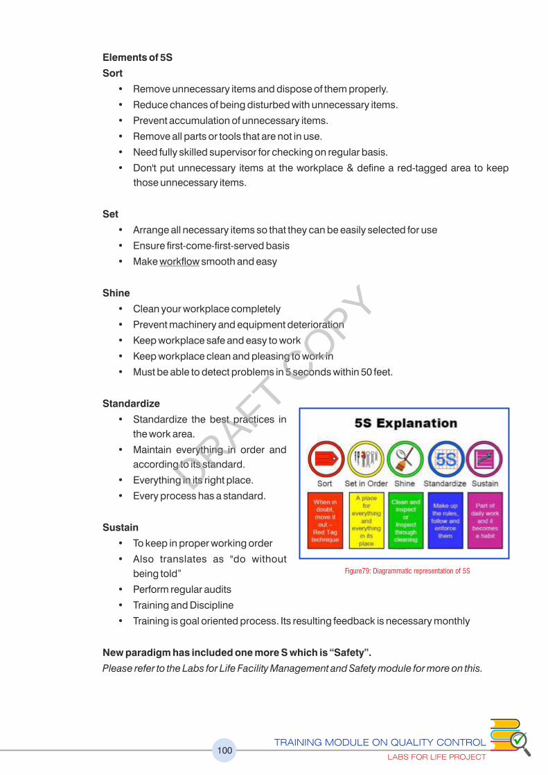
TRAINING MODULE ON QUALITY CONTROL
LABS FOR LIFE PROJECT100
Elements of 5S
Sort
• Remove unnecessary items and dispose of them properly.
• Reduce chances of being disturbed with unnecessary items.
• Prevent accumulation of unnecessary items.
• Remove all parts or tools that are not in use.
• Need fully skilled supervisor for checking on regular basis.
• Don't put unnecessary items at the workplace & define a red-tagged area to keep
those unnecessary items.
Set
• Arrange all necessary items so that they can be easily selected for use
• Ensure first-come-first-served basis
• Make workow smooth and easy
Shine
• Clean your workplace completely
• Prevent machinery and equipment deterioration
• Keep workplace safe and easy to work
• Keep workplace clean and pleasing to work in
• Must be able to detect problems in 5 seconds within 50 feet.
Standardize
• Standardize the best practices in
the work area.
• Maintain everything in order and
according to its standard.
• Everything in its right place.
• Every process has a standard.
Sustain
• To keep in proper working order
• Also translates as "do without
being told”
• Perform regular audits
• Training and Discipline
• Training is goal oriented process. Its resulting feedback is necessary monthly
New paradigm has included one more S which is “Safety”.
Please refer to the Labs for Life Facility Management and Safety module for more on this.
Figure79: Diagrammatic representation of 5S
DRAFT COPY

TRAINING MODULE ON QUALITY CONTROL
LABS FOR LIFE PROJECT101
Areas where 5S can apply in a Lab
• Lab Safety
• Lab Quality
• Equipment Management
• Documentation
• Others
5.4 Failure Modes and Effects Analysis (FMEA) Tool
Failure Modes and Effects Analysis (FMEA) is a systematic, proactive method for evaluating a
process to identify where and how it might fail and to assess the relative impact of different
failures, in order to identify the parts of the process that are most in need of change. FMEA
includes review of the following:
Steps in the process
• Failure modes (What could go wrong?)
• Failure causes (Why would the failure happen?)
• Failure effects (What would be the consequences of each failure?)
Teams use FMEA to evaluate processes for possible failures and to prevent them by
correcting the processes proactively rather than reacting to adverse events after failures
have occurred. This emphasis on prevention may reduce risk of harm to samples, patients
and staff. FMEA is particularly useful in evaluating a new process prior to implementation and
in assessing the impact of a proposed change to an existing process.
Failure Modes and Effects Analysis (FMEA) was developed outside of health care and is now
being used in health care to assess risk of failure and harm in processes and to identify the
most important areas for process improvements.
An example of using FMEA in the lab:
I d e n t i f y a p r o c e s s t h a t n e e d s
improvement
Identify the components and classify it on
a grid (in rows)
Include the following in columns:
Occurrence (Occ), Severity (Sev),
Detection (Det), and Risk Priority Number
(RPN). Add responsibility, action take,
and approximate date for closure also
into the columns
In the following example of pre-analytical
process in being analyzed
Following the thoughts above, it is clear that a needle stick injury or spillage is self-evident,
easily detected, reported and gets a higher score for Det. However, the severity (Sev) is
Figure 80: Diagrammatic representation of FMEA
DRAFT COPY

TRAINING MODULE ON QUALITY CONTROL
LABS FOR LIFE PROJECT102
higher for needle stick as the hazards are more. A hemolysis is less easily reported if the staff
is not trained, and includes the risk of erroneous reports. Micro clots which results in probe
block, wrong results is even less easily reported. These two can be high in occurrence if the
collection practice is compromised. After plotting the grades on the grid, multiply the 3
captured numbers so as to derive the RPN or Risk Priority Number to decide on the priority of
interventions. Decide on the course of action and assign responsibility. Track all the risk
factors as Quality Indicators.
The Detection (Det.) is deleted in many analysis (see below) as it may bring down the RPN
spuriously. Only Occurrence and Severity are considered. Not being able to detect the risk
factors is not to the advantage.
FMEA can be used simultaneously with a Fishbone matrix and Risk Prioritization matrix
in understanding and eliminating risks
Process Mode
Occurrence 1-10
Detection 1-10
SeverityRPN =
(Occ*Det* Sev)
Action Responsibility
Needle stick
Spillage
Hemolysis
Wrong Container
Inadequate Volume
Micro clots
XYZ
3
2
7
2
1
8
2
9
8
3
7
3
5
1
10
8
8
8
6
8
3
270
128
168
132
18
320
6
Training, PEP
Training,Engineering Controls
Training,Adequate Phlebotomy
equipment
Training
Training,Volume Checks
Equipment Maintenance,Training
ABC
HOD, QM
HOD, QM
QM
QM
QM
QM
Senior Technician
A fishbone diagram is typically used in root cause
analysis. It can also be used for risk analysis.
A fishbone chart of all pre-analytical process is
made. 4 key points, requisition, sample
collection, transportation, sample set up
(accessioning) and analysis have been mapped.
Any process can thus be mapped.
DRAFT COPY

TRAINING MODULE ON QUALITY CONTROL
LABS FOR LIFE PROJECT103
Each activity of the process is graded from 0-1 as per
chances of occurrence
Each activity of the process is graded from 0-1 as
per severity
A risk prioritization matrix or occurrence severity
matric is used to plot the grades
The data from the pre-analytical process of the
above lab is plotted as shown. Areas falling in the
red region has to be prioritized for action
The relationship between Corrective Action,
Preventive action, Risk Management and Six Sigma.
Both Preventive action plan and Risk management
are ident ica l . The la t ter though is more
comprehensive in that, each process needs to be
subjected to the analysis systematically
Figure 81: Illustrative examples of FMEA & Risk Analysis
DRAFT COPY

TRAINING MODULE ON QUALITY CONTROL
LABS FOR LIFE PROJECT104
5.5 Pareto Principle
The Pareto principle (also known as the 80–20 rule, the law of the vital few, and the principle of
factor sparsity) states that, for many events, roughly 80% of the effects come from 20% of the
causes. E.g. 80% of your problems occurs come from 20% of your defects.
It is also called: Pareto diagram, Pareto analysis
Variations: weighted Pareto chart, comparative Pareto charts
A Pareto chart is a bar graph. The lengths of the bars represent frequency or cost (time or
money), and are arranged with longest bars on the left and the shortest to the right. In this
way the chart visually depicts which situations are more significant.
Many businesses have an easy access to dramatic improvements in profitability by focusing
on the most effective areas and eliminating, ignoring, automating, delegating or retraining
the rest, as appropriate. What could be the 20% of the issues in communication that results in
80% of the outcomes?
Pareto charts typically show the frequency of occurrence of a variable of interest in different
categories arranged in order of descending frequency. The focus is generally on the
category that has the highest frequency of occurrence, but in some cases, this typical
frequency-based portrait of data is not appropriate. Focusing on the frequency of occurrence
of an event is appropriate when the degree of importance is the same for all categories and
when the potential for occurrence is the same for all categories. When the frequency
approach is not appropriate, the procedure to be used depends on which of these two
conditions is not satisfied.
When to Use a Pareto Chart
• When analyzing data about the frequency of problems or causes in a process.
• When there are many problems or causes and you want to focus on the most significant.
• When analyzing broad causes by looking at their specific components.
• When communicating with others about your data.
Pareto Chart Procedure
1. Decide what categories you will use to group items.
2. Decide what measurement is appropriate. Common measurements are frequency,
quantity, cost and time.
3. Decide what period of time the Pareto chart will cover: One work cycle? One full
day? A week?
4. Collect the data, recording the category each time. (Or assemble data that already exist.)
5. Subtotal the measurements for each category.
6. Determine the appropriate scale for the measurements you have collected. The
maximum value will be the largest subtotal from step 5. (If you will do optional steps 8
and 9 below, the maximum value will be the sum of all subtotals from step 5.) Mark the
scale on the left side of the chart.
DRAFT COPY
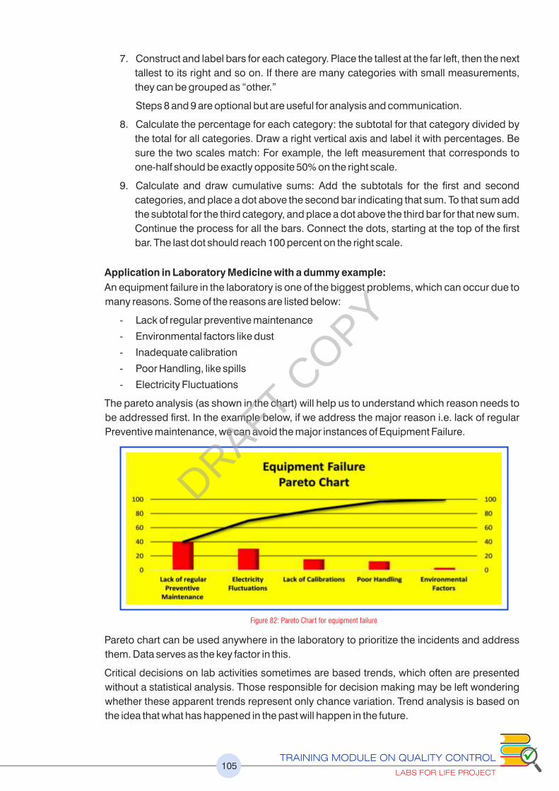
TRAINING MODULE ON QUALITY CONTROL
LABS FOR LIFE PROJECT105
7. Construct and label bars for each category. Place the tallest at the far left, then the next
tallest to its right and so on. If there are many categories with small measurements,
they can be grouped as “other.”
Steps 8 and 9 are optional but are useful for analysis and communication.
8. Calculate the percentage for each category: the subtotal for that category divided by
the total for all categories. Draw a right vertical axis and label it with percentages. Be
sure the two scales match: For example, the left measurement that corresponds to
one-half should be exactly opposite 50% on the right scale.
9. Calculate and draw cumulative sums: Add the subtotals for the first and second
categories, and place a dot above the second bar indicating that sum. To that sum add
the subtotal for the third category, and place a dot above the third bar for that new sum.
Continue the process for all the bars. Connect the dots, starting at the top of the first
bar. The last dot should reach 100 percent on the right scale.
Application in Laboratory Medicine with a dummy example:
An equipment failure in the laboratory is one of the biggest problems, which can occur due to
many reasons. Some of the reasons are listed below:
- Lack of regular preventive maintenance
- Environmental factors like dust
- Inadequate calibration
- Poor Handling, like spills
- Electricity Fluctuations
The pareto analysis (as shown in the chart) will help us to understand which reason needs to
be addressed first. In the example below, if we address the major reason i.e. lack of regular
Preventive maintenance, we can avoid the major instances of Equipment Failure.
Pareto chart can be used anywhere in the laboratory to prioritize the incidents and address
them. Data serves as the key factor in this.
Critical decisions on lab activities sometimes are based trends, which often are presented
without a statistical analysis. Those responsible for decision making may be left wondering
whether these apparent trends represent only chance variation. Trend analysis is based on
the idea that what has happened in the past will happen in the future.
Figure 82: Pareto Chart for equipment failure
DRAFT COPY

TRAINING MODULE ON QUALITY CONTROL
LABS FOR LIFE PROJECT106
5.6 Trend Analysis
Why Do Trend Analysis
• Comparing one time period to another time period
• Comparing one group to another
• Making future projections
• Comparing with other organizations
Applications in Laboratory Medicine with an example
- Consumptions of Reagents over a period (daily, weekly, monthly, and annually)
- Peer group analysis (EQAS reporting) – comparison with many labs
- To observe patient load in laboratory department wise, test wise etc.
- To see the trend of CV of various parameters to see the quality
How to do trend Analysis
- It is one of the easy and simple techniques used. Data is collected over a period of time
and is plotted on charts. The trends are observed to take a decision accordingly.
Application of Trend analysis in laboratory, single analyte
CV trend analysis, multiple analytes, multiple months.
The figure below shows a set of data of CVs of analytes which are arranged analyte-wise and
month-wise. Consistently high CVs in Creatinine are seen, pointing towards a consistent
imprecision, possibly implying a reagent defect. A root cause analysis needs to be done. A
sudden increase in the CVs is seen in April pointing to some shift in the equipment
performance and warranting root cause analysis. A room temperature rise, an equipment
malfunction such as probe issues, storage temperature of multiple reagents pointing a
refrigerator malfunction etc. need to be considered.
Figure 83: Graphical representation of Trend Analysis of single parameter over a period of one year
DRAFT COPY

TRAINING MODULE ON QUALITY CONTROL
LABS FOR LIFE PROJECT107
0
2
4
6
8
10
12
14
Glucose Urea Creatinine Cholesterol
Jan
Fab
Mar
Apr
0
2
4
6
8
10
12
14
Jan Feb Mar Apr
Glucose
Urea
Creatinine
Cholesterol
Figure 84: Graphical representation of Trend Analysis of multiple parameters over a period of time, both parameter wise and month wise
5.7 Root cause analysis (RCA) & Cause & Effect Analysis
• Root Cause Analysis (RCA) is a structured
method used to analyze incidents and
adverse events. Initially developed to
analyze industrial accidents, RCA is now
widely deployed as an error analysis tool in
health care.
• A root cause is an initiating cause of either a
condition or a causal chain that leads to an
outcome or effect of interest. Commonly,
root cause is used to describe the depth in
the causal chain where an intervention
could reasonably be implemented to
improve performance or prevent an
undesirable outcome.Figure 85: Fishbone diagram
DRAFT COPY

TRAINING MODULE ON QUALITY CONTROL
LABS FOR LIFE PROJECT108
As example, imagine a day in the lab with the very high workload of samples, and the
major equipment broke down. An investigation into the machine that stopped
because it was overloaded and the fuse blew. Investigation shows that the machine
overloaded because it had a bearing that wasn't being sufficiently lubricated. The
investigation proceeds further and finds that the automatic lubrication mechanism
had a pump which was not pumping sufficiently, hence the lack of lubrication.
Investigation of the pump shows that it has a worn shaft. Investigation of why the shaft
was worn discovers that there isn't an adequate mechanism to prevent metal scrap
getting into the pump. This enabled scrap to get into the pump, and damage it. The
root cause of the problem is therefore that metal scrap can contaminate the
lubrication system. Fixing this problem ought to prevent the whole sequence of
events recurring. Compare this with an investigation that does not find the root cause:
replacing the fuse, the bearing, or the lubrication pump will probably allow the
machine to go back into operation for a while. But there is a risk that the problem will
simply recur, until the root cause is dealt with.
In India, one of the causes for recurrent equipment breakdown is dust and lack of
proper maintenance.
The primary aim of root cause analysis is:
• To identify the factors that resulted in the nature, the magnitude, the location, and the
timing of the harmful outcomes (consequences) of one or more past events; to determine
what behaviors, actions, inactions, or conditions need to be changed; to prevent
recurrence of similar harmful outcomes; and to identify lessons that may promote the
achievement of better consequences. ("Success" is defined as the near-certain
prevention of recurrence.)
• To be effective, root cause analysis must be performed systematically, usually as part of
an investigation, with conclusions and root causes that are identified backed up by
documented evidence. A team effort is typically required.
• There may be more than one root cause for an event or a problem, wherefore the difficult
part is demonstrating the persistence and sustaining the effort required to determine
them.
• The purpose of identifying all solutions to a problem is to prevent recurrence at lowest
cost in the simplest way. If there are alternatives that are equally effective, then the
simplest or lowest cost approach is preferred.
• The root causes identified will depend on the way in which the problem or event is
defined. Effective problem statements and event descriptions (as failures, for example)
are helpful and usually required to ensure the execution of appropriate analyses.
DRAFT COPY

TRAINING MODULE ON QUALITY CONTROL
LABS FOR LIFE PROJECT109
Corrective Actions
Ishikawa Charts (Fish Bone) Ask the 5 Why's Identify problems
Problem
People Methods
Materials Environment Measurements
Figure 86: Using a Fishbone tool
Four Major Steps in RCA
The RCA is a four-step process involving the following:
1. Data collection.
2. Causal factor charting
3. Root cause identification.
4. Recommendation generation and implementation.
Value Stream Mapping
Value Stream Mapping (VSM) is following a product’s production path from beginning to
end. In the case of a lab, it is a sample. Wasteful or non-value adding aspects are: confusion,
unnecessary motion/conveyance (physical movement required to get a simple task
accomplished and to move people and products from place to place), waiting, over-
processing (doing more activities than is necessary to complete a piece of work), inventory
issues (obsolete, duplicated, unnecessary, or missed items), defects (errors) and
overproduction (an example, redundant paperwork). All these wasteful activities can occur
along the sample path in a lab.
A proper Value Stream Mapping along the sample path creates value, eliminates waste,
reduces lead time and in turn reduces, total costs. The following are a few examples of the
results of a VSM in a lab, increasing productivity
Reducing analytical batch sizes and increasing the frequency of analyses
Middleware to interface instrumentation with the LIMS
Staggering shifts
Cross training analysts for reporting
Automation of manual analyses
So it is vital that the staff and management of a laboratories undertake VSM to enhance the
performance and avoid mistakes.
DRAFT COPY

TRAINING MODULE ON QUALITY CONTROL
LABS FOR LIFE PROJECT110
The above processes will enable the laboratory to identify bottlenecks and avoid &
mitigate risks. Though many of the techniques seem self-evident and easily doable,
unless the laboratory invests time and efforts into practicing these, several hidden
problems will never come into view resulting in unforeseen breakdowns and risks
jeopardizing the safety of the patients, reports, and staff.
DRAFT COPY

TRAINING MODULE ON QUALITY CONTROL
LABS FOR LIFE PROJECT111
REFERENCESChapter 1: Introduction
1. Statistical Quality Controls and Method Evaluation Training Curriculum developed by CDC
Atlanta, 2016
2. ISO 15189: 2012 Medical laboratories — Requirements for quality and competence
3. Laboratory Quality Management System: Training Toolkit, 2009, 2015
Chapter 2: Internal Controls Quantitative (Statistical Qcs)
1. Statistical Quality Controls and Method Evaluation Training Curriculum developed by
CDC Atlanta, 2016
2. https://www.westgard.com
3. http://www.bio-rad.com/en-us/product/qcnet
4. Laboratory Quality Management System: Training Toolkit, 2015
5. ISO 15189: 2012 Medical laboratories — Requirements for quality and competence
6. C 24 A3: Statistical Quality Control for Quantitative Measurement Procedures, Principles and
Definitions, Approved Guideline 3rd Edition
7. G 104: Guide to estimation of Measurement Uncertainty In Testing, American Association for
laboratory Accreditation
8. Tietz Textbook of Clinical Chemistry and Molecular Diagnostics, 5th Edition
9. Recommended Total Allowable Error Limits, Sun Pharma Total + Allowable + Error + Limits
+ Table+Example_rev20120725%20(3).pdf
10. Total Analytical Error AACC.org.html
11. Tonk’s Rule: Establishing Performance Standards, A Practical Approach, David G Rhoads
12. CLIA Proficiency Testing Criteria for Acceptable PerformanceCLIAC MeetingSeptember 1,
2010, Rex Astles, PhD, DABCC, FACB, Laboratory Practice Standards Branch, Division of
Laboratory Science and Standards
13. Sigma Metrics in Clinical Laboratories, From Theory to Practice, Dr Dana Baily, University Of
Toronto, Gamma DynaCare
14. Bull’s Algorithm: Quality Control in Clinical Laboratories, Petros Karkalousos1 and Angelos
Evangelopoulos, Technological Institute of Athens, Faculty of Health and Caring
Professions, Department of Medical Laboratories Lab Organization & Quality Control dept,
Roche Diagnostics (Hellas) S.A. Athens, Greece
15. Automated Hematology Analyzer, XS series, XS-1000i/XS-800i, Instructions for Use
16. NABL 112 Specific Criteria for Accreditation of Medical Laboratories, 4th Issue, 2016
Chapter 3: Proficiency Testing / External Quality Assurance
1. Statistical Quality Controls and Method Evaluation Training Curriculum developed by CDC
Atlanta, 2016
2. ISO 15189: 2012, Medical laboratories — Requirements for quality and competence
3. Randox EQAS: http://www.randox.com/riqas-external-quality-assessment/
DRAFT COPY
TRAINING MODULE ON QUALITY CONTROL
LABS FOR LIFE PROJECT112
4. Bio Rad EQAS: http://www.bio-rad.com/en-us/product/qcnet
5. NEQAS: National Aids Research Institute
6. VIS Scoringhttps://www.scribd.com/presentation/214063561/EQAS-Interpretation
Chapter 4: Method Evaluation
1. Statistical Quality Controls and Method Evaluation Training Curriculum developed by CDC
Atlanta, 2016
2. ISO 15189: 2012, Medical laboratories — Requirements for quality and competence
3. https://www.westgard.com
4. What is the difference between Co-efficient of Determination and Coefficient of Correlation?
Guarav Bansal EW Green Bay
5. NABL 112 Specific Criteria for Accreditation of Medical Laboratories, 4th Issue, 2016
6. CLSI Guidelines C28-A3: Defining, Establishing and Verifying Reference Intervals In the
Clinical Laboratory, Approved Guidelines
Chapter 5:General Concepts in Quality Assurance
1. Dennis, Pascal. Lean Production Simplified: A Plain Language Guide to the World’s Most
Powerful Production Systems. Productivity Press, 2002
2. http://www.balancedscorecard.org/bkgd/
3. http://www.hci.com.au/hcisite2/toolkit/
4. http://www.isixsigma.com/
5. RISK AND THE MEDICAL LABORATORY Michael A Noble MD FRCPC, Chair, Program Office
for Laboratory Quality Management, University of British Columbia - Vancouver BC
6. Risk Management in the Medical Laboratory: Reducing Risk through Application of
Standards Michael A Noble MD FRCPC, Chair, Program Office for Laboratory Quality
Management, University of British Columbia - Vancouver BC
OPY
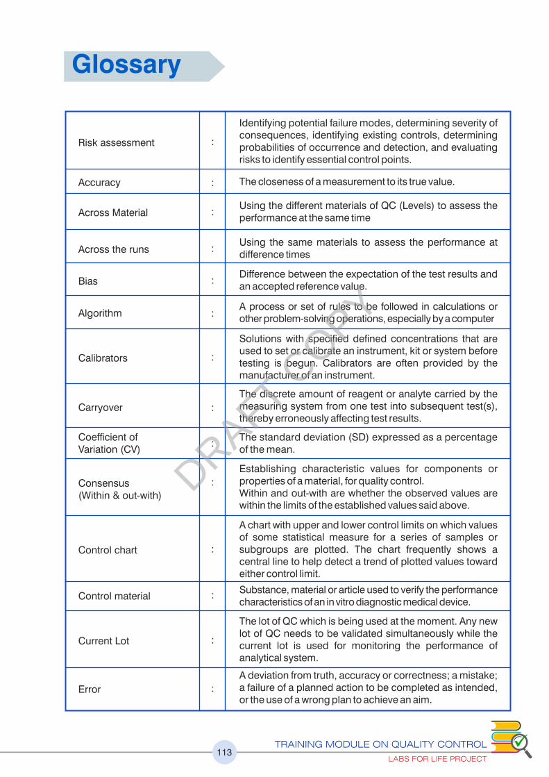
TRAINING MODULE ON QUALITY CONTROL
LABS FOR LIFE PROJECT113
Identifying potential failure modes, determining severity of consequences, identifying existing controls, determining probabilities of occurrence and detection, and evaluating risks to identify essential control points.
The closeness of a measurement to its true value.
Using the different materials of QC (Levels) to assess the performance at the same time
Using the same materials to assess the performance at difference times
Difference between the expectation of the test results and an accepted reference value.
A process or set of rules to be followed in calculations or other problem-solving operations, especially by a computer
Solutions with specified defined concentrations that are used to set or calibrate an instrument, kit or system before testing is begun. Calibrators are often provided by the manufacturer of an instrument.
The discrete amount of reagent or analyte carried by the measuring system from one test into subsequent test(s), thereby erroneously affecting test results.
The standard deviation (SD) expressed as a percentage of the mean.
Establishing characteristic values for components or properties of a material, for quality control. Within and out-with are whether the observed values are within the limits of the established values said above.
Risk assessment :
:
:
:
:
:
:
:
:
:
:
:
:
:
Accuracy
Across Material
Across the runs
Bias
Algorithm
Calibrators
Carryover
Coefficient of Variation (CV)
Consensus (Within & out-with)
Control chart
A chart with upper and lower control limits on which values of some statistical measure for a series of samples or subgroups are plotted. The chart frequently shows a central line to help detect a trend of plotted values toward either control limit.
Substance, material or article used to verify the performance characteristics of an in vitro diagnostic medical device.
The lot of QC which is being used at the moment. Any new lot of QC needs to be validated simultaneously while the current lot is used for monitoring the performance of analytical system.
A deviation from truth, accuracy or correctness; a mistake; a failure of a planned action to be completed as intended, or the use of a wrong plan to achieve an aim.
Control material
Current Lot
Error
Glossary
DRAFT COPY

TRAINING MODULE ON QUALITY CONTROL
LABS FOR LIFE PROJECT114
:
:
:
:
:
:
:
:
:
:
:
:
:
:
:
A system for objectively checking the laboratory’s performance using an external agency or facility.
A property exhibited by appropriately preserved biological material, on repeated analysis, whereby the data points show normal distribution i.e. 68-95-99 rule.
A method of assuring comparability of tests done using different mechanism or machines, which may employ different methods and have different traceability of calibrators.
Freeze dried material which require reconstitution before use.
A stated mean for a control material as defined by the manufacturer of the material. This requires to be verified in the lab before being used to verify the performance of an analytical system
The mean observed by the lab while running a QC for a defined period of time. Also called obtained/lab mean.
An ongoing process whereby the system is checked for fitness for use.
Closeness of agreement between quantity values obtained by replicate measurements of a quantity, under specified conditions. See Quantitative examination.
Concerns monitoring all operations of the laboratory.
Relating to, measuring, or measured by the quality of something rather than its quantity
relating to, measuring, or measured by the quantity of something rather than its quality
Defining the analytical goals of a laboratory. This is the responsibility of the laboratory head. Also termed as a Quality requirements.
The necessary infrastructure or foundational building blocks in any organization that need to be in place and functioning effect ively in order to support the organization’s work operations so that they proceed smoothly. See Quality management. CLSI developed the quality management framework and organized the topics as the "12 Quality System Essentials" based on both ISO 15189 and CLSI GP26-A3 documents.
It is the range of test values expected for a designated population in which 95% of the individuals are presumed to be healthy (or normal). In some analytes reference interval have been replaced by decision limits established by international consensus. Also called BRI (Biological reference interval)/BRR (Biological reference range).
The analyte being measured by the measuring system
External quality assessment (EQA)
Gaussian Distribution
Harmonization
Lyophilized
Manufacturer’s Mean
Measurand
Observed Mean
Performance Evaluation
Precision
Process control
Qualitative
Quality system essentials
Quantitative
Reference Interval
Quality Specification
DRAFT COPY

TRAINING MODULE ON QUALITY CONTROL
LABS FOR LIFE PROJECT115
:
:
:
:
:
:
:
:
:
:
:
:
:
The identification, analysis and economic control of those risks which can threaten the assets or earnings of an enterprise.
A factor that caused a nonconformity and should be permanently eliminated through process improvement.
Deciding on using single rule or multi rules and which rules to use depending on the performance of the analyte.
Test whose results are expressed as a rough estimate of how much of the measured substance is present.
Sensitivity is the lowest concentration of an analyte that can be measured. This is also LoD/LoQ
Artifactual increase or decrease of quantity of analyte due to the presence of any interfering substance(s).
Methods and techniques used to generate, analyze, interpret and present data.
Length of time that a sample’s final result may be issued to the ordering physician.
Confirmation, through provision of objective evidence, that the requirements for a specific intended use or application have been fulfilled.
Values of analytes which is significant clinically. May be high, low or normal. Other terms used are Medical Decision Values (MDV), Clinical Decision points (CDP), Clinical Decision Values (CDV).
Confirmation, through provision of objective evidence, that specified requirements have been fulfilled.
Using the same QC material across runs.
Using the different QC material in a run.
Risk management
Root Cause
Rule Selection
Semi quantitative examination
Sensitivity
Specificity
Statistical tools
Turnaround time
Validation
Medical Decision Points
Verification
Within Material
Within Run DRAFT COPY

TRAINING MODULE ON QUALITY CONTROL
LABS FOR LIFE PROJECT116
ADA : American Diabetes Association
AMR : Analytical Measurement range
AON : Average of Normal
ASC : Atypical Squamous cells
BRR : Biological Reference Range
BRI : Biological Reference Interval
BV : Biological Variations
CCV : Chosen Coefficient of Variation
CLIA : Clinical Laboratory Improvement Amendments
CLSI : Clinical and Laboratory Standards Institute
CV : Coefficient of Variation
CVI : Coefficient of Variation Index
DV : Designated Value
ELISA : enzyme-linked immunosorbent assay
EQAS : External Quality Assurance Scheme
FDA : Food & Drug Administration
FIFO : First in First Out
FMEA : Failure Mode Effect Analysis
IFU : Instruction for Use
IHC : Immuno- Histo Chemistry
ILC : Inter-laboratory Comparison
INR : International Normalized Ratio
IQC : Internal Quality Control
ISI : International Standardization Index
ISO : The International organization for Standardization
JIT : Just in Time
LJ : Levey Jennings
LoD : Limit of Detection
LoQ : Limit of Quantification
Abbreviations
DRAFT COPY
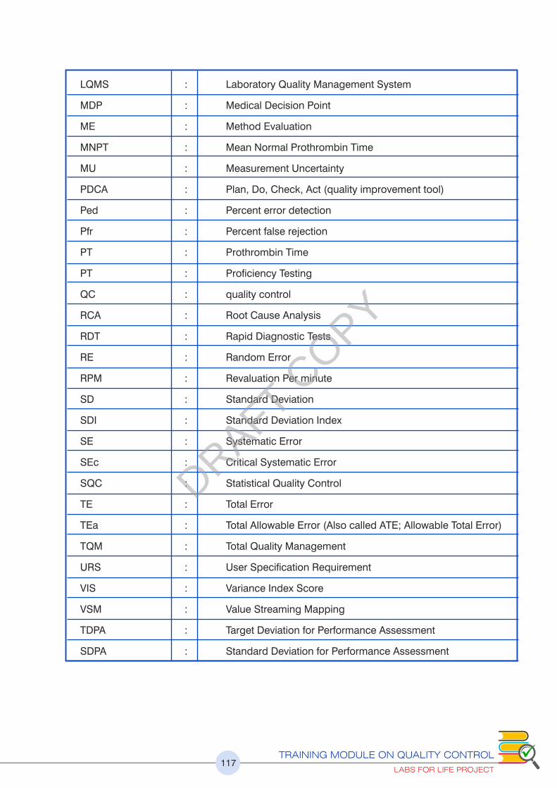
TRAINING MODULE ON QUALITY CONTROL
LABS FOR LIFE PROJECT117
LQMS : Laboratory Quality Management System
MDP : Medical Decision Point
ME : Method Evaluation
MNPT : Mean Normal Prothrombin Time
MU : Measurement Uncertainty
PDCA : Plan, Do, Check, Act (quality improvement tool)
Ped : Percent error detection
Pfr : Percent false rejection
PT : Prothrombin Time
PT : Proficiency Testing
QC : quality control
RCA : Root Cause Analysis
RDT : Rapid Diagnostic Tests
RE : Random Error
RPM : Revaluation Per minute
SD : Standard Deviation
SDI : Standard Deviation Index
SE : Systematic Error
SEc : Critical Systematic Error
SQC : Statistical Quality Control
TE : Total Error
TEa : Total Allowable Error (Also called ATE; Allowable Total Error)
TQM : Total Quality Management
URS : User Specification Requirement
VIS : Variance Index Score
VSM : Value Streaming Mapping
TDPA : Target Deviation for Performance Assessment
SDPA : Standard Deviation for Performance Assessment
DRAFT COPY

118
Annexure
Job-Aids
A. Equations
B. Creating a L-J Chart
C. Navigating the Westgard Internet Site (www.westgard.com)
D. Steps for Developing a QC Strategy
E. General Guidelines for Proficiency Testing
Annexure 1
Annexure 2
Annexure 3
Annexure 4
Annexure 5
Annexure 6
Annexure 7
Annexure 8
Total Allowable Error Limits
A. BV Desirables
B. CLIA Limits
C. Recommended TEa Limits (Sun Diagnostic)
Medical Decision Points
(Extracts from Westgard site)
Sigma-Metrics QC Selection Tool
A. Sigma-Metrics QC Selection Tool for 2 Levels Control
B. Sigma-Metrics QC Selection Tool for 3 Levels Control
Frequency and Scope of Testing: Commonly used EQAS Schemes
Corrective Action Formats for IQC & EQA
A. Corrective Action formats for IQC
B. Corrective Action formats for EQA (PT Failure Checklist)
Evaluation Summary Report
Worksheets
DRAFT COPY

TRAINING MODULE ON QUALITY CONTROL
LABS FOR LIFE PROJECT119
Job-Aids Annexure 1
DRAFT COPY

TRAINING MODULE ON QUALITY CONTROL
LABS FOR LIFE PROJECT120
DRAFT COPY

TRAINING MODULE ON QUALITY CONTROL
LABS FOR LIFE PROJECT121
B. Creating an L-J Chart
DRAFT COPY

TRAINING MODULE ON QUALITY CONTROL
LABS FOR LIFE PROJECT122
C. Navigating the Westgard Internet Site (www.westgard.com)
DRAFT COPY

TRAINING MODULE ON QUALITY CONTROL
LABS FOR LIFE PROJECT123
D. Steps for Developing a QC Strategy
1. Select a test.
2. Select appropriate control materials.
3. Determine your TE limitsA
a. Select the TEA for the test; note the resources used for the selection.
b. Select the Target Value (Clinical Decision Concentration) for each control; note the
resource used for the selection.
c. Calculate the TEA in units.
4. Determine current method performance
a. Calculate the current method’s mean from a stable system for each control.
b. Calculate the current method’s SD from a stable system for each control.
c. Calculate the SEc and Sigma-metric for each control; if SEc is zero or a negative number,
then your TE ��TE . Stop reporting patient results immediately, verify your four Key A
Numbers of Quality, and fix the problem(s)
5. Select appropriate control rules
a. Choose the appropriate Sigma-metrics QC Selection Tool for the number of controls used
for the test.
b. Locate the Sigma-metric value on the Sigma-scale (scale at the top of the X-axis).
c. Validate the Sigma-metric against the SEc scale (scale at the bottom of the X-axis).
d. Draw a vertical line from the Sigma-metric value to the SEc value.
e. Assess probability of error rejection where the Sigma line intersects with the QC rule
power curve.
f. Identify candidate QC rules in which Ped is ��0.90 (90%).
g. Assess false rejection rates of candidate QC rules from the table [��0.05 (5%)].
h. Select the appropriate QC rule and total number of control measurements (N) that
provide the lowest cost and are easiest to implement.
6. On-going monitoring of QC
a. Create the QC chart.
b. Determine how often a supervisor will review the QC chart, depending on the SEc or
Sigma-metric.
c. Initiate corrective action if SEc and Sigma are low.
d. Develop a standardized process to investigate QC rule violations from daily, summary,
and peer-reviewed QC data.
e. Monitor the accuracy, precision, SEc, and Sigma at least on a monthly basis.
f. Take corrective actions as needed; continue to target poorly-performing analytical systems.
7. Document this entire process.
8. Educate the analytical staff.
9. Communicate with upper management regarding the laboratory’s needs for a
complete QC process.
DRAFT COPY

TRAINING MODULE ON QUALITY CONTROL
LABS FOR LIFE PROJECT124
E. General Guidelines for Proficiency Testing
Laboratory proficiency testing (PT) is an essential element of laboratory quality assurance.
Proficiency testing is an independent and unbiased assessment that evaluates the laboratory’s
ability to produce correct answers. Proficiency testing provides an assessment of the validity of
testing in your laboratory.
Handling Your PT Survey
Pre-analytical
Note the date of receipt for your shipment
Immediately inspect and reconcile the contents of your shipment with the
accompanying paperwork
Are all required specimens available?
Is the quality and appearance of the specimens acceptable?
Store the shipment properly
Note due date of results
Reconstitute specimens with volumetric pipettes and correct diluent
Mix samples well before analyzing
Analytical
Analyze specimens at correct temperature. If shipment was stored in the refrigerator,
specimens may need to come to room temperature before testing.
Always refer to your survey instructions for storage and specimen handling.
Analyze PT specimens in the same fashion as patient specimens.
Do not refer any PT samples to another laboratory, even if your instrument is non-
functioning or is part of your testing algorithm.
Rotate testing responsibility for PT specimens between all laboratory personnel that are
routinely performing the analysis in your laboratory.
Perform PT analysis well before due date of results.
Post-Analytical
Assure that your laboratory’s results are reported according to the PT provider’s instructions.
Ensure the proper method and instrument code are recorded for each test so that you are
part of the correct peer group.
If test not performed is the correct answer because of equipment issues, then indicate this
on the form.
If the result obtained requires additional testing per your laboratory’s algorithm, then
indicate on the form to be sent to a reference laboratory or further testing required, but do
not actually send the PT sample to another laboratory.
Review results for clerical errors on answer sheet, including decimal point placement.
DRAFT COPY
TRAINING MODULE ON QUALITY CONTROL
LABS FOR LIFE PROJECT125
Retain a copy of answer sheet for your records. Attach all raw data and the instrument
print-out to the answer sheet.
If possible, retain specimens in freezer for confirmatory testing if needed.
If you use the PT sample materials to cross-check other instrument or methods, or as part
of your competency training program, then be absolutely sure the PT results are
submitted to the PT provider before starting these activities.
Receipt of Results
Review your results with your peer grouping.
Investigate all unacceptable grades.
Have the Laboratory Director and Supervisor review, and sign and date results.
Review results with testing personnel. Retain a copy for competency assessment and
place into personnel record.
Investigate any failed responses and complete an EQA Failure Checklist assessment.
Follow-up with remedial actions if indicated.
DRAFT COPY

TRAINING MODULE ON QUALITY CONTROL
LABS FOR LIFE PROJECT126
Total Allowable Error LimitsA. BV
Desirable Specification: Page1 (Sample)
Annexure 2
DRAFT COPY
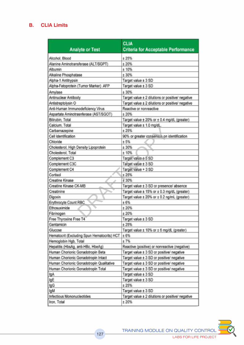
TRAINING MODULE ON QUALITY CONTROL
LABS FOR LIFE PROJECT127
B. CLIA Limits
DRAFT COPY

TRAINING MODULE ON QUALITY CONTROL
LABS FOR LIFE PROJECT128
DRAFT COPY

C. Recommended TEa Limits (Sun Diagnostic)
TRAINING MODULE ON QUALITY CONTROL
LABS FOR LIFE PROJECT129
DRAFT COPY

TRAINING MODULE ON QUALITY CONTROL
LABS FOR LIFE PROJECT130
Medical Decision Points(Sample from Westgard site)
Medical Decision Levels
These tables of medical decision levels provide possible critical decision levels - where
you can assess performance (CV, bias) and determine the Sigma-metrics and appropriate
QC procedures.
Clinical Decision levels for Electrolytes, Metabolites, Proteins and Enzymes, Hormones,
Hematology related tests and Drugs are available. Electrolytes are shown as an example here
Annexure 3
DRAFT COPY

TRAINING MODULE ON QUALITY CONTROL
LABS FOR LIFE PROJECT131
Sigma-Metrics QC Selection
Tools for 2 & 3 Levels Control
A. Sigma-Metrics QC Selection Tool for 2 Levels Control
Annexure 4
DRAFT COPY

TRAINING MODULE ON QUALITY CONTROL
LABS FOR LIFE PROJECT132
B. Sigma-Metrics QC Selection Tool for 3 Levels Control
DRAFT COPY
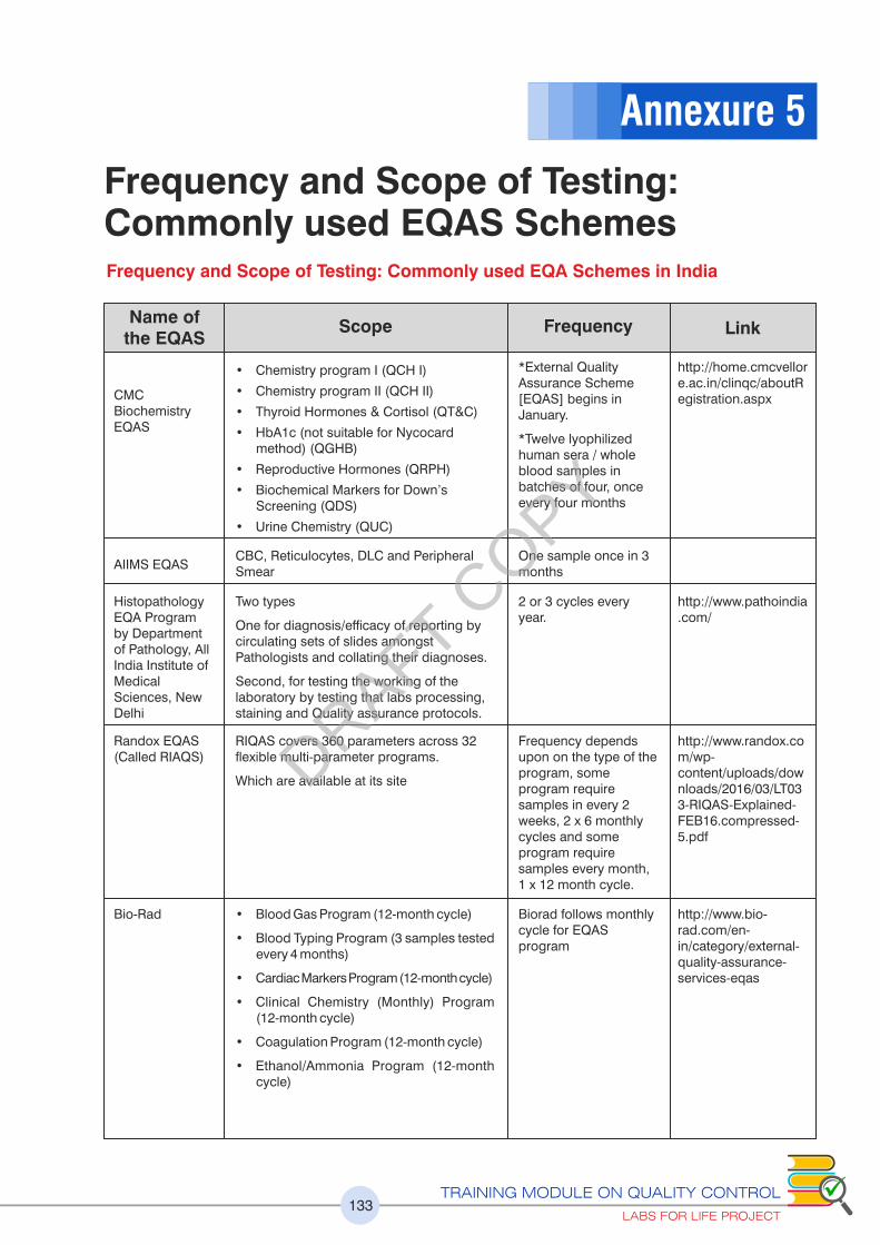
TRAINING MODULE ON QUALITY CONTROL
LABS FOR LIFE PROJECT133
Frequency and Scope of Testing: Commonly used EQAS SchemesFrequency and Scope of Testing: Commonly used EQA Schemes in India
Name of the EQAS
Scope Frequency Link
CMC Biochemistry EQAS
• Chemistry program I (QCH I)
• Chemistry program II (QCH II)
• Thyroid Hormones & Cortisol (QT&C)
• HbA1c (not suitable for Nycocard method) (QGHB)
• Reproductive Hormones (QRPH)
• Biochemical Markers for Down’s Screening (QDS)
• Urine Chemistry (QUC)
*External Quality Assurance Scheme [EQAS] begins in January.
*Twelve lyophilized human sera / whole blood samples in batches of four, once every four months
http://home.cmcvellore.ac.in/clinqc/aboutRegistration.aspx
AIIMS EQASCBC, Reticulocytes, DLC and Peripheral Smear
One sample once in 3 months
Histopathology EQA Program by Department of Pathology, All India Institute of Medical Sciences, New Delhi
Randox EQAS (Called RIAQS)
Bio-Rad
Two types
One for diagnosis/efficacy of reporting by circulating sets of slides amongst Pathologists and collating their diagnoses.
Second, for testing the working of the laboratory by testing that labs processing, staining and Quality assurance protocols.
RIQAS covers 360 parameters across 32 exible multi-parameter programs.
Which are available at its site
2 or 3 cycles every year.
Frequency depends upon on the type of the program, some program require samples in every 2 weeks, 2 x 6 monthly cycles and some program require samples every month, 1 x 12 month cycle.
Biorad follows monthly cycle for EQAS program
http://www.pathoindia.com/
http://www.randox.com/wp-content/uploads/downloads/2016/03/LT033-RIQAS-Explained-FEB16.compressed-5.pdf
http://www.bio-rad.com/en-in/category/external-quality-assurance-services-eqas
• Blood Gas Program (12-month cycle)
• Blood Typing Program (3 samples tested every 4 months)
• Cardiac Markers Program (12-month cycle)
• Clinical Chemistry (Monthly) Program (12-month cycle)
• Coagulation Program (12-month cycle)
• Ethanol/Ammonia Program (12-month cycle)
Annexure 5
DRAFT COPY

TRAINING MODULE ON QUALITY CONTROL
LABS FOR LIFE PROJECT134
Bio-Rad
CMC Hemostasis EQAS
CMC Transfusion Medicine EQAS:
Biorad follows monthly cycle for EQAS program
2 Samples Quarterly
One sample once in 3 months
http://www.bio-rad.com/en-in/category/external-quality-assurance-services-eqas
https://www.cmceqas.org/registration.php
https://www.cmceqas.org/registration.php
• Hematology Program (12-month cycle consisting of 4 separate shipments)
• Hemoglobin Program (12-month cycle)
• HIV/Hepatitis Program
• Immunoassay (Monthly) Program
• Lipids Program (12-month cycle)
• Serum Proteins Program
• Syphilis Program
• Therapeutic Drug Monitoring Program
• ToRCH/EBV/MuMZ Program
• Urinalysis Program
• Urine Chemistry Program
Program A:
• Prothrombin time (PT)/INR
• Activated thromboplastin time (APTT)
• Fibrinogen
• Thrombin time (TT)
Program B
• Factor VIII Assay
• Factor IX Assay
• Von Willebrand factor study
• (RICOF & VWF: Ag)
Program A (For Laboratories)
• Blood Grouping and Typing
Program B (For Laboratories)
• Blood Grouping and Typing
• Direct Coombs and Indirect Coombs test
Program C (For Blood Bank)
• Blood Grouping and Typing
• Direct Coombs and Indirect Coombs test
• Compatibility test
Program D(For Blood Bank)
• Blood Grouping and Typing
• Direct Coombs and Indirect Coombs test
• Compatibility test
• Antibody Screening
• Antibody Identification
Blood Bank External Quality Assessment Scheme (BEQAS)
The frequencies of distribution of samples are 3 cycles per year. (First cycle-January, Second cycle-July, Third cycle-November)
http://nabh.co/Images/pdf/EQAS-ApplicationForm.pdf
• HBsAg
• Anti-HIV
• Anti-HCV
• NAT (HBV / HCV / HIV-1,HIV- 2,HIV-O,HIV-M)
• VDRL
DRAFT COPY
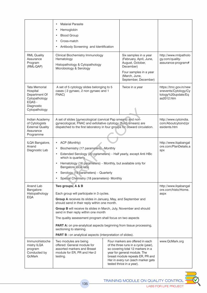
TRAINING MODULE ON QUALITY CONTROL
LABS FOR LIFE PROJECT135
RML Quality Assurance Program(RML-QAP)
Six samples in a year (February, April, June, August, October, December)
Four samples in a year (March, June, September, December)
http://www.rmlpathology.com/quality-assurance-program#
• Malarial Parasite
• Hemoglobin
• Blood Group
• Cross-match
• Antibody Screening and Identification
• ACP (Monthly)
• Biochemistry (17 parameters) –Monthly
• Extended Serology (20 parameters) – Half yearly, except Anti HBc which is quarterly
• Hematology (16 parameters) – Monthly, but available only for Bangalore local labs
• Serology (18 parameters) – Quarterly
• Special Chemistry (18 parameters)- Monthly
Clinical Biochemistry Immunology Hematology
Histopathology & Cytopathology Microbiology & Serology
Tata Memorial Hospital Department Of Cytopathology EQAS - Diagnostic Cytopathology
Immunohistochemistry ILQA program Conducted by QcMark
Twice in a year
Four markers are offered in each of the three runs in a cycle (year), so covering total 12 markers in a year for general module. The breast module repeats ER, PR and Her in every run (each marker gets tested thrice in a year).
https://tmc.gov.in/newsnevents/Cytology/Cytology%20update/Eqas2012.htm
www.QcMark.org
A set of 5 cytology slides belonging to 5 cases ( 2 gynaec, 2 non gynaec and 1 FNAC)
Two modules are being offered: General module for assorted markers and Breast module for ER, PR and Her-2 testing.
Indian Academy of Cytologists External Quality Assurance Programme
http://www.cytoindia.com/Aboutcytoind/presidents.htm
A set of slides [gynecological (cervical Pap smears) and non-gynecological, FNAC and exfoliative cytology (uid) smears) are dispatched to the first laboratory in four groups for onward circulation.
Two groups; A & B
Each group will participate in 3 cycles.
Group A receives its slides in January, May, and September and should send in their reply within one month.
Group B will receive its slides in March, July, November and should send in their reply within one month
The quality assessment program shall focus on two aspects
PART A: on pre-analytical aspects beginning from tissue processing, sectioning to staining.
PART B : on analytical aspects (interpretation of slides).
ILQA Bangalore, Anand Diagnostic Lab
http://www.ilqabangalore.com/PlanDetails.aspx
Anand Lab Bangalore: Histopathology EQA
http://www.ilqabangalore.com/histo/Home.aspx
DRAFT COPY

TRAINING MODULE ON QUALITY CONTROL
LABS FOR LIFE PROJECT136
This scheme involves distribution of for quality control packages to be sent during the months of January, April, July and October of every year
a) Staining: Gram staining/AFB staining/Leishman staining for Malarial parasites.
b) Culture: General bacteriology ID (Manual/Automated) up to species level and antimicrobial susceptibility (Kirby Bauer/MIC method).
c) Serology:
Antibodies to HIV 1&2
Antibodies to HCV
HBs Ag test
Widal test
CRP
RA Factor
ASO
RPR
Medical Mycology
It assesses three major aspects of parasitic diagnosis namely
1) Microscopy 2) Serology 3) Molecular biology.
IAMM EQAS
The Society for Indian Human and Animal Mycologists (SIHAM) through PGIMER, Chandigarh
IATP External Quality Assurance in Parasitic Diagnosis through JIPMER, Puducherry
http://www.ilqabangalore.com/
http://www.siham.in/Media/eqas_in_medical_mycology.pdf
http://iatp.in/
Syphilis testing by RPR / VDRL / TPHA Gonorrhea Gram Staining/ Antibiotic Susceptibility
CD4 (Flow Cytometry) – 2 samples thrice in year
HIV:8 samples twice yr
STI
NARI
Once a year
Cd4 (Flow Cytometry) – 2 samples thrice in year HIV: 8 samples twice in a year
http://www.nari-icmr.res.in/
EQA of the NRLs will be conducted by WHO Supra-National Reference Laboratories. Proficiency testing of DST by the Culture and DST laboratories is conducted at the time of accreditation by the respective designated NRL.
The Culture and DST laboratories should send a list of all cultures to NRLs, who would randomly select ten cultures for proficiency testing. These cultures would be then sent to NRLs by 37 Culture and DST laboratories and the result of NRLs will be communicated to the laboratories with corrective actions, if required.
In addition, NRLs will send a set of 20 cultures to the laboratories at the time of accreditation and annually thereafter, and the results will be compared and suggestions for improvement would be provided, if required.
EQAS under RNTCP
DRAFT COPY

TRAINING MODULE ON QUALITY CONTROL
LABS FOR LIFE PROJECT137
http://www.ukneqas.org.uk/documents/UKNEQAScompendiumfinal%283%29.pdf
NEQAS now comprises a network of 390 schemes operating from 26 centers based at major hospitals, research institutions and universities throughout the UK. The services cover qualitative and interpretative investigations in reproductive science, cellular pathology, clinical chemistry, genetics, hematology, immunology and microbiology.
UK NEQAS
http://www.rcpaqap.com.au
http://www.rcpaqap.com.au/wpcontent/uploads/2016/02/2016_Product_Catalogue.pdf
Chemical Pathology Group/Program
Hematology and Transfusion Group/Program : Hematology & Transfusion
Infectious Diseases and Immunology Group/Program: Immunology, Microbiology, Serology, Biosecurity & Synovial Fluid
Cellular and Tissue Pathology Group/Program: Anatomical Pathology, Cytopathology Program,
Royal College of Pathologists of Australasia Quality Assurance Programs
DRAFT COPY

TRAINING MODULE ON QUALITY CONTROL
LABS FOR LIFE PROJECT138
Corrective Action Formats for IQC & EQA
IQC Corrective Action
Date
Analyte
QC Lot no & Expiry
QC Level:
Rule/Rules Violated
Check Storage/Expiry of
Reagent
Calibrator
QC
Check Environment
Temperature
Humidity
Check Operator
If problem persists, top testing, call service personnel
Comments
Signature of Technician
Sigma
QC Rules for Analyte
Troubleshooting and Corrective actions
Annexure 6
DRAFT COPY

TRAINING MODULE ON QUALITY CONTROL
LABS FOR LIFE PROJECT139
B. Corrective Action formats for EQA (PT Failure Checklist)
Assessment Review
PT Report Reviewed for Clerical Errors: Evaluation results match your copy of submitted results Yes No N/A
Wrong Data Entered Yes No N/A
Wrong Units Reported Yes No N/A
Incorrect instrument or methodology indicated Yes No N/A
Sample Handling: Unexpected delays in receiving survey Yes No N/A
Kit contents correct and in acceptable condition Yes No N/A
Testing performed within suggested instructional time guidelines Yes No N/A
Specimens stored at correct temperature between receipt and analysis Yes No N/A
Specimen analyzed at correct temperature Yes No N/A
Sample mixed properly before testing Yes No N/A
Sample diluted properly Yes No N/A
Special Handling instructions were followed Yes No N/A
Testing Procedure: Testing Personnel competent to perform analysis Yes No N/A
Manufacturer's package insert available and followed Yes No N/A
Testing procedure properly followed Yes No N/A
Kit components replaced from other kits Yes No N/A
Sample mix-up Yes No N/A
Samples demonstrate a matrix effec Yes No N/A
Instrument recently calibrated or due for calibration Yes No N/A
Instrument maintenance up-to-date Yes No N/A
New lot number of reagents or calibrators used Yes No N/A
Reagents within expiration date Yes No N/A
Results reported within linearity Yes No N/A
QC within established range Yes No N/A
QC demonstrates an even distribution around the mean Yes No N/A
QC results show a shift, trend, or bias Yes No N/A
Manufacturer consulted Yes No N/A
Sample Results: A single sample fails on several analytes Yes No N/A
All samples failed for the analyte Yes No N/A
Previous survey results for the analyte demonstrate a problem emerging Yes No N/A
PT material reassayed Yes No N/A
Survey Name: Clinical Specialty:
Specimens: Date:
Problem Description:
Proficiency Testing Failure Checklist
DRAFT COPY

TRAINING MODULE ON QUALITY CONTROL
LABS FOR LIFE PROJECT140
Survey Name: Clinical Specialty:
Specimens: Date:
Investigation:
Proficiency Testing Failure Checklist
Conclusion:
Corrective Action Taken:
Laboratory Director Review
DRAFT COPY

TRAINING MODULE ON QUALITY CONTROL
LABS FOR LIFE PROJECT141
Evaluation Summary Report Purpose: Verification of Manufacturer’s Claims / Change Controls
Description of Equipment / Process:
Equipment/Process:
Serial Number/ Equipment ID: Reference
Serial Number/ Equipment ID: Test
Date:
FDA Approval Status: Approved / not approved
Procedure: Ref to Lab QSP: Method Evaluation…..
Results: All raw data reports and statistical analysis details can be found in the file numbers
1. Precision – refer to file number
Analyte:
MDP Manufacturer’s Precision Claim
33% of CLIA Normal Control /Sample CV%
Abn Control /Sample CV%
Acceptability
Expected Results Observed Results
Between Day
MDP Manufacturer’s Precision Claim
25% of CLIA Normal Control /Sample CV%
Abn Control /Sample CV%
Acceptability
Expected Results Observed Results
Within Run
Annexure 7
DRAFT COPY

TRAINING MODULE ON QUALITY CONTROL
LABS FOR LIFE PROJECT142
2. Accuracy: refer to file number
Analyte :
Total Allowable Error with Source:
Results a) r value
b) Slope
c) Intercept
d) Graph interpretation of Difference and % Difference
MDP Y’ % Bias %TE Sigma Acceptability
3. Linearity: refer to file number
a) Total Allowable Error and Source
b) % of Allowable Error used for calculations
c) Graphical Interpretation of Linearity
d) Linearity
e) AMR
f) CRR
Assigned Value at Dilution
Mean Y’ % Diff % Limit Acceptability
Analytical Measurement Range (AMR) and Clinical Reportable Range (CRR)
Analyte Mfg’s AMRLow Value
VerifiedHigh Value
VerifiedLinearity Validated
AMRDilutions CRR
DRAFT COPY
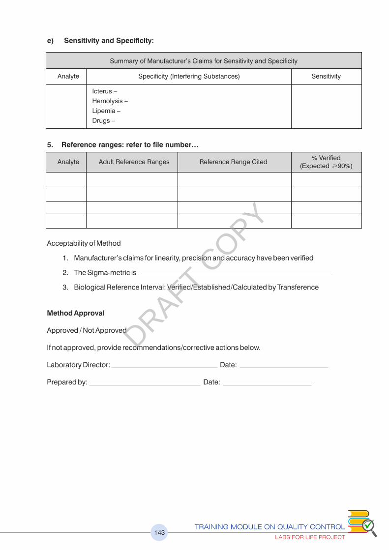
TRAINING MODULE ON QUALITY CONTROL
LABS FOR LIFE PROJECT143
e) Sensitivity and Specificity:
Summary of Manufacturer’s Claims for Sensitivity and Specificity
Analyte Specificity (Interfering Substances) Sensitivity
Icterus –
Hemolysis –
Lipemia –
Drugs –
5. Reference ranges: refer to file number…
Analyte Adult Reference Ranges% Verified
(Expected �90%)Reference Range Cited
Acceptability of Method
1. Manufacturer’s claims for linearity, precision and accuracy have been verified
2. The Sigma-metric is
3. Biological Reference Interval: Verified/Established/Calculated by Transference
Method Approval
Approved / Not Approved
If not approved, provide recommendations/corrective actions below.
Laboratory Director: Date:
Prepared by: Date:
DRAFT COPY

TRAINING MODULE ON QUALITY CONTROL
LABS FOR LIFE PROJECT144
WORKSHEETS
Exercise 1: Find the Mean, Median and Mode
Mean Mode Median
A. 2,2,2,2,42,2,2,2,2,2,2
B. 9, 2,3,4,11,5,8,6,7,5
C. 6,6,6,6,6,6,6,6,6,6,6
Exercise 2.68-95-99 rule for Gaussian
Data set A: Mean 90, SD 3.2
Assign the graph with +_3SD numbers & Plot the data on the graph: Is it Gaussian?
* 93, 84,90,93,88,86,88,95,92,94,88,90,89,87,91,90,94,88,97,90,91,95,90,85,91,94,89.91,85,89
+3s
+2s
+1s
X
-1s
-2s
-3s
Data Set B: Mean: 52, SD 24
Assign the graph with +_3SD numbers & Plot the data on the graph: Is it Gaussian?
45,48,41,49,102,44,43,141,44,46,43,43,45,49,41,42,40,43,48,43
Annexure 8
DRAFT COPY

TRAINING MODULE ON QUALITY CONTROL
LABS FOR LIFE PROJECT145
+3s
+2s
+1s
X
-1s
-2s
-3s
3. Calculate Mean and SD and Range
- 5.1, 5.3, 4.9, 5.1, 5.4, 5.1, 5.6, 5.4
- 2.13, 2.09, 2.10, 2.11, 2.15
- 36.83, 35.79, 37.01, 35.72, 36.29, 36.33, 36.54, 36.48, 36.91, 35.87
Exercise 4. LJ Plotting with two levels of QC
Plot the LJ with given values:
Following are the data points for Level 1 QC of AST for the month of September 2016. Please
define mean, SD (3SD), range and plot the values on the graph.
Data Set A:
Data Set B:
Following are the data points for Level II QC of AST for the month
Data Set B:
Following are the data points for Level II QC of AST for the month of September 2016. Please define
mean, SD (3SD), range and plot the values on the graph.
DRAFT COPY
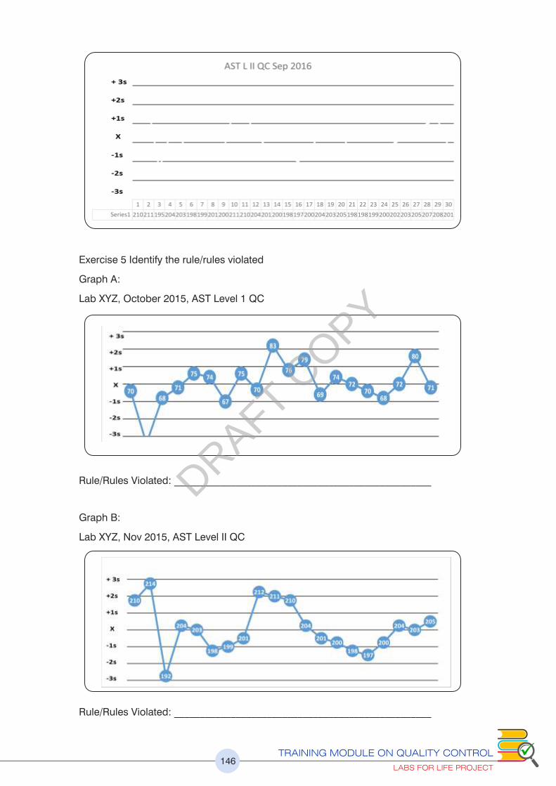
TRAINING MODULE ON QUALITY CONTROL
LABS FOR LIFE PROJECT146
Exercise 5 Identify the rule/rules violated
Graph A:
Lab XYZ, October 2015, AST Level 1 QC
Graph B:
Lab XYZ, Nov 2015, AST Level II QC
Rule/Rules Violated: __________________________________________________
Rule/Rules Violated: __________________________________________________
DRAFT COPY
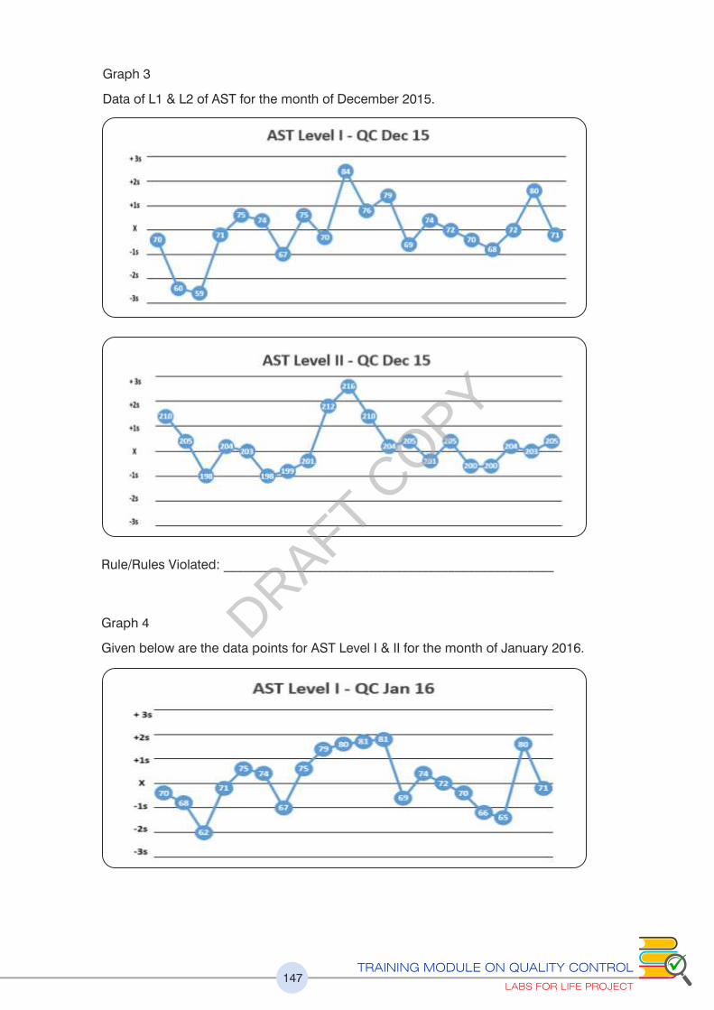
TRAINING MODULE ON QUALITY CONTROL
LABS FOR LIFE PROJECT147
Graph 3
Data of L1 & L2 of AST for the month of December 2015.
Rule/Rules Violated: __________________________________________________
Graph 4
Given below are the data points for AST Level I & II for the month of January 2016.DRAFT C
OPY
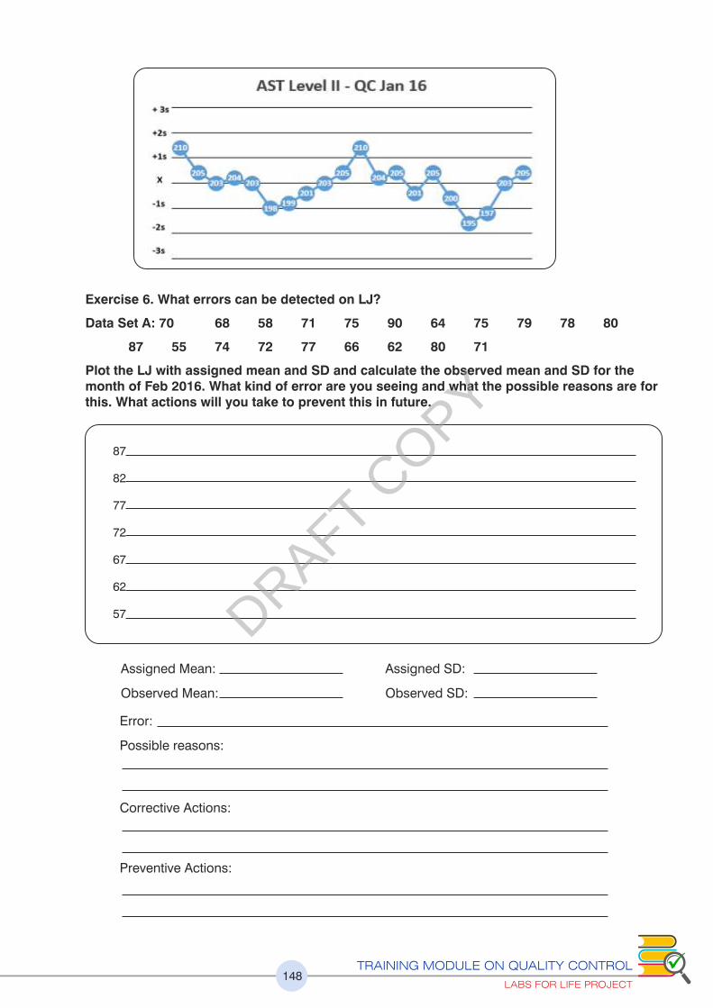
TRAINING MODULE ON QUALITY CONTROL
LABS FOR LIFE PROJECT148
Exercise 6. What errors can be detected on LJ?
Data Set A: 70 68 58 71 75 90 64 75 79 78 80
87 55 74 72 77 66 62 80 71
Plot the LJ with assigned mean and SD and calculate the observed mean and SD for the month of Feb 2016. What kind of error are you seeing and what the possible reasons are for this. What actions will you take to prevent this in future.
87
82
77
72
67
62
57
Assigned Mean:
Observed Mean:
Assigned SD:
Observed SD:
Error:
Possible reasons:
Corrective Actions:
Preventive Actions:
DRAFT COPY
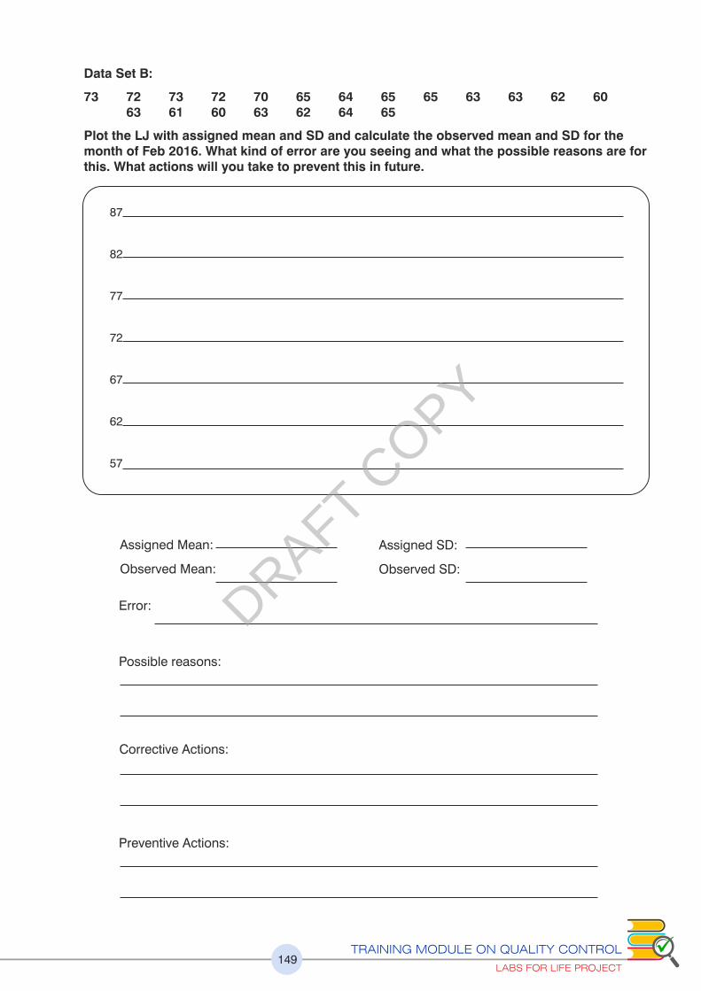
TRAINING MODULE ON QUALITY CONTROL
LABS FOR LIFE PROJECT149
Data Set B:
73 72 73 72 70 65 64 65 65 63 63 62 60 63 61 60 63 62 64 65
Plot the LJ with assigned mean and SD and calculate the observed mean and SD for the month of Feb 2016. What kind of error are you seeing and what the possible reasons are for this. What actions will you take to prevent this in future.
87
82
77
72
67
62
57
Assigned Mean:
Observed Mean:
Assigned SD:
Observed SD:
Error:
Possible reasons:
Corrective Actions:
Preventive Actions:
DRAFT COPY

TRAINING MODULE ON QUALITY CONTROL
LABS FOR LIFE PROJECT150
Exercise 7: Calculating CV percentage
The following are the data points for Level I & II for AST for the month of January 2015 for Lab XYZ.
Data Set A:
70 68 62 71 75 74 67 75 79 80 81 81 69
74 72 70 66 65 80 71 70 79 79 65 71
68 70 72 70 70
Mean
SD
CV%:
Data Set B:
210 205 203 204 203 198 199 201 203 205 210 204 205
201 205 200 195 197 203 205 198 198 199 200 202
203 205 207 208 201
Mean
SD
CV%:
Exercise 8: New Lot QC
Scenario A: You have a new lot of QC no 12345. For AST Level II, the manufacturer’s mean is 220 IU/L and range is 190-250 IU/L. You have done parallel testing and got these values. Plot your lab’s chart for Lot No. 12345 for AST, before you would assign a new range and new mean.
210 205 203 204 203 198 199 201 203 205 210 204 205
201 205 200 195 197 203 205 198 198 199 200 202
203 205 207 208 201
What will be the Lab assigned mean and range?
Manufacturer’s mean: 220 IU/L Lab Mean
Manufacturer’s Range: 19-250 IU/L Lab Range
+3s
+2s
+1s
X
-1s
-2s
-3s
DRAFT COPY

TRAINING MODULE ON QUALITY CONTROL
LABS FOR LIFE PROJECT151
Scenario B:
Scenario A: You have a new lot of QC no 12345. For AST Level II, the manufacturer’s mean is 220
IU/L and range is 190-250 IU/L. You could not do the parallel testing in full because QC was
supplied late. You have accumulated 8 data points over 4 days as shown below. CV% for AST in
the running/current lot 12344 is 4%. Plot your lab’s chart for Lot No. 12345 for AST, before you
would assign a new lab range and lab mean.
What will be the Lab assigned mean and range?
Manufacturer’s mean: 220 IU/L Lab Mean ______________
Manufacturer’s Range: 19-250 IU/L Lab Range ______________
Exercise 9: Right and Wrong LJ Chart
For the data given below for Level 1 AST control, four charts have been plotted. Out of them one is
correct and others are wrong (marked accordingly). Identify the problem in the charts and the
consequences of using wrong charts. Specific inputs are to be given for the circled data points.
+3s
+2s
+1s
X
-1s
-2s
-3s
No. of run Values
1 202
2 205
3 210
4 204
5 203
6 201
7 199
8 194
Mean
SD
CV %
DRAFT COPY

TRAINING MODULE ON QUALITY CONTROL
LABS FOR LIFE PROJECT152
Exercise 9: Right and Wrong LJ Chart
For the data given below for Level 1 AST control, four charts have been plotted. Out of them one is
correct and others are wrong (marked accordingly). Identify the problem in the charts and the
consequences of using wrong charts. Specific inputs are to be given for the circled data points.
DRAFT COPY

Exercise 11: Total Error (TE), %TE
For the data given below, calculate the % CV, Total Error (TE), %TE.
Data of Glucose & AST for the month of November 2015 is
TRAINING MODULE ON QUALITY CONTROL
LABS FOR LIFE PROJECT153
Exercise 10: Bias, Absolute Bias, % Bias
For the data given below, calculate Bias, Absolute Bias,, % Bias.
Data of Glucose & AST for the month of November 2015 is
Glucose AST
Lab Mean 95 203
Peer group Mean 90 197
Bias
Absolute Bias
% Bias
Glucose AST
Lab Mean 95 203
Peer group Mean 90 197
SD 4 6
% CV
Absolute Bias
% Bias
TE
%TE
Exercise 12: Total Allowable error and judging acceptability of the analyte performance
Find the TE using CLIA proficiency limits from annexure and compare with the total error in the A
above cases and judge acceptability of the analyte performance.
Glucose AST
%TE
% TE from CLIA A
Judging Acceptability
DRAFT COPY
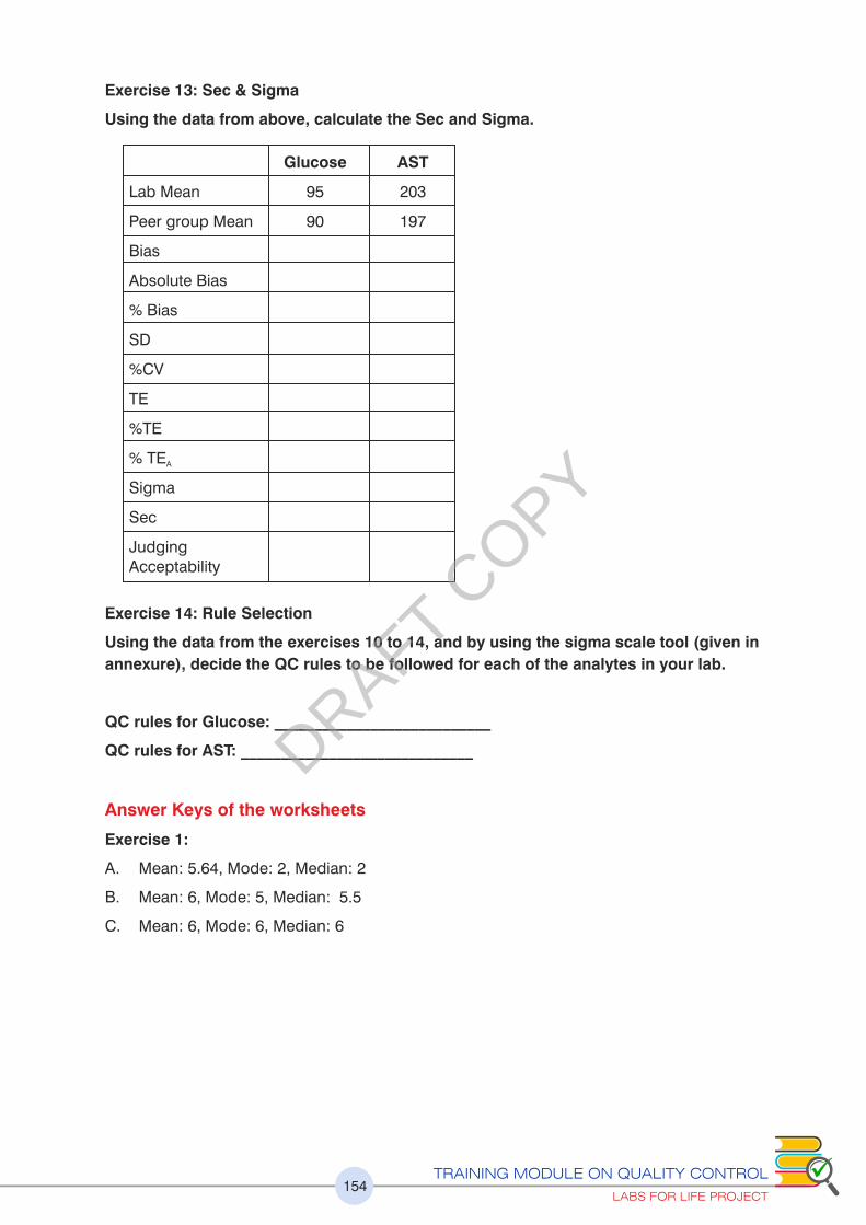
TRAINING MODULE ON QUALITY CONTROL
LABS FOR LIFE PROJECT154
Exercise 13: Sec & Sigma
Using the data from above, calculate the Sec and Sigma.
Glucose AST
Lab Mean 95 203
Peer group Mean 90 197
Bias
Absolute Bias
% Bias
SD
%CV
TE
%TE
% TE A
Sigma
Sec
Judging Acceptability
Exercise 14: Rule Selection
Using the data from the exercises 10 to 14, and by using the sigma scale tool (given in
annexure), decide the QC rules to be followed for each of the analytes in your lab.
QC rules for Glucose: ___________________________
QC rules for AST: _____________________________
Answer Keys of the worksheets
Exercise 1:
A. Mean: 5.64, Mode: 2, Median: 2
B. Mean: 6, Mode: 5, Median: 5.5
C. Mean: 6, Mode: 6, Median: 6
DRAFT COPY

TRAINING MODULE ON QUALITY CONTROL
LABS FOR LIFE PROJECT155
Exercise 2:
Graph .1
.
YES THIS IS GAUSSIAN
Graph .2
These numbers will not form a Gaussian pattern. A -2SD is a negative number. The mean
and median are far apart
Exercise 3
Exercise 4
Data Set A B C
Mean 5.24 2.1 36.38
SD 0.23 0.02 0.47
Upper End 5.92 2.19 37.78
Lower End 4.56 2.04 34.97
Data Set A Data Set B:
Mean 72.4 202.5
SD 4.3 4.4
Upper End 85.3 215.7
Lower End 59.5 189.3
DRAFT COPY
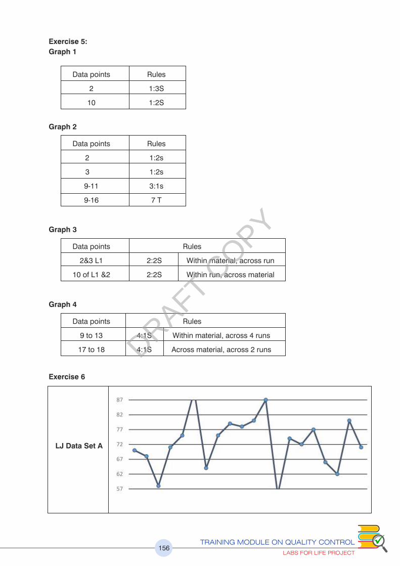
TRAINING MODULE ON QUALITY CONTROL
LABS FOR LIFE PROJECT156
Exercise 5:
Graph 1
Data points Rules
2 1:3S
10 1:2S
Graph 2
Data points Rules
2 1:2s
3 1:2s
9-11 3:1s
9-16 7 T
Graph 3
Data points Rules
2&3 L1 2:2S Within material, across run
10 of L1 &2 2:2S Within run, across material
Graph 4
Data points Rules
9 to 13 4:1S Within material, across 4 runs
17 to 18 4:1S Across material, across 2 runs
Exercise 6
LJ Data Set A
DRAFT COPY
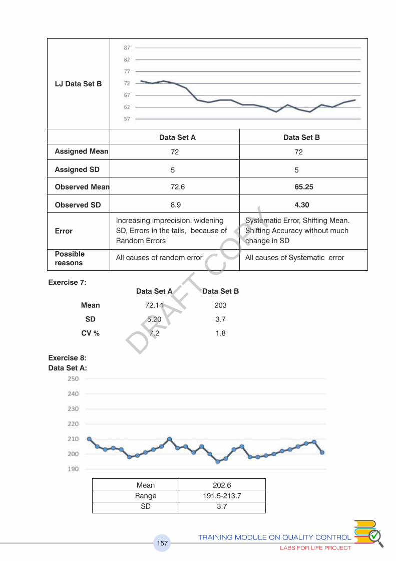
TRAINING MODULE ON QUALITY CONTROL
LABS FOR LIFE PROJECT157
LJ Data Set B
Assigned Mean
Assigned SD
Observed Mean
Observed SD
Error
Possible reasons
Data Set A Data Set B
72
5
72.6
8.9
Increasing imprecision, widening
SD, Errors in the tails, because of
Random Errors
All causes of random error
72
5
65.25
4.30
Systematic Error, Shifting Mean.
Shifting Accuracy without much
change in SD
All causes of Systematic error
Exercise 7: Data Set A Data Set B
Mean 72.14 203
SD 5.20 3.7
CV % 7.2 1.8
Exercise 8:
Data Set A:
Mean 202.6
Range 191.5-213.7
SD 3.7
DRAFT COPY
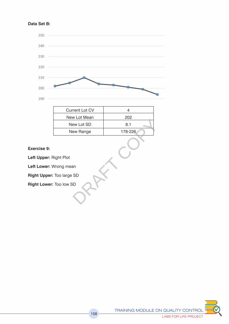
TRAINING MODULE ON QUALITY CONTROL
LABS FOR LIFE PROJECT158
Data Set B:
Current Lot CV 4
New Lot Mean 202
New Lot SD 8.1
New Range 178-226
Exercise 9:
Left Upper: Right Plot
Left Lower: Wrong mean
Right Upper: Too large SD
Right Lower: Too low SD
DRAFT COPY

TRAINING MODULE ON QUALITY CONTROL
LABS FOR LIFE PROJECT159
Exercises 10 to 14
Data Set A Data Set B:
Lab Mean 95 203
Peer group Mean 90 197
Bias 5 6
Absolute Bias 5 6
% Bias 5.6 3.0
SD 4 6
%CV 4.2 3.0
TE 11.6 15.9
%TE 12.5 7.9
% TEa 10 20
Sigma 1.1 5.7
SEc - 4.1
Judging Acceptability Not Acceptable Good Performance
Rule Selection Change Method Single Rule
DRAFT COPY


