Neural Networks 21 (2008) 427–436www.elsevier.com/locate/neunet

2008 Special Issue

Training neural network classifiers for medical decision making: The effectsof imbalanced datasets on classification performanceI

Maciej A. Mazurowskia,∗, Piotr A. Habasa, Jacek M. Zuradaa, Joseph Y. Lob, Jay A. Bakerb,Georgia D. Tourassib

a Computational Intelligence Lab, Department of Electrical and Computer Engineering, University of Louisville, Louisville, KY 40292, USAb Duke Advanced Imaging Laboratories, Department of Radiology, Duke University Medical Center, Durham, NC 27705, USA

Received 9 August 2007; received in revised form 2 December 2007; accepted 11 December 2007

Abstract

This study investigates the effect of class imbalance in training data when developing neural network classifiers for computer-aided medicaldiagnosis. The investigation is performed in the presence of other characteristics that are typical among medical data, namely small training samplesize, large number of features, and correlations between features. Two methods of neural network training are explored: classical backpropagation(BP) and particle swarm optimization (PSO) with clinically relevant training criteria. An experimental study is performed using simulated dataand the conclusions are further validated on real clinical data for breast cancer diagnosis. The results show that classifier performance deteriorateswith even modest class imbalance in the training data. Further, it is shown that BP is generally preferable over PSO for imbalanced training dataespecially with small data sample and large number of features. Finally, it is shown that there is no clear preference between oversampling and nocompensation approach and some guidance is provided regarding a proper selection.c© 2007 Elsevier Ltd. All rights reserved.

Keywords: Classification; Feed-forward neural networks; Class imbalance; Computer-aided diagnosis

1. Introduction

In computer-aided decision (CAD) systems, computeralgorithms are used to help a physician in diagnosing apatient. One of the most common tasks performed by a CADsystem is the classification task where a label is assignedto a query case (i.e., a patient) based on a certain numberof features (i.e., clinical findings). The label determines thequery’s membership in one of predefined classes representingpossible diagnoses. CAD systems have been investigated andapplied for the diagnosis of various diseases, especially forcancer. Some comprehensive reviews on the topic can be foundin Kawamoto, Houlihan, Balas, and Lobach (2005), Lisboa andTaktak (2006) and Sampat, Markey, and Bovik (2005). CAD

I An abbreviated version of some portions of this article appeared inMazurowski, Habas, Zurada, and Tourassi (2007) as part of the IJCNN 2007Conference Proceedings, published under IEE copyright.

∗ Corresponding address: 407 Lutz Hall, University of Louisville, Louisville,KY 40222, USA. Tel.: +1 502 852 3165; fax: +1 502 852 3940.

E-mail address: maciej.mazurowski@louisville.edu (M.A. Mazurowski).

0893-6080/$ - see front matter c© 2007 Elsevier Ltd. All rights reserved.doi:10.1016/j.neunet.2007.12.031

systems rely on a wide range of classifiers, such as traditionalstatistical and Bayesian classifiers (Duda, Hart, & Stork, 2000),case-based reasoning classifiers (Aha, Kibler, & Albert, 1991),decision trees (Mitchell, 1997), and neural networks (Zhang,2000). In particular, neural network classifiers are a verypopular choice for medical decision making and they have beenshown to be very effective in the clinical domain (Lisboa, 2002;Lisboa & Taktak, 2006).

To construct a classifier, a set of examples representingprevious experience is essential. In general, the larger and morerepresentative the set of available examples is, the better theclassification of future query cases (Raudys & Jain, 1991).In the medical domain, however, there are several challengesand practical limitations associated with data collection. First,collecting data from patients is time consuming. Second,acquiring large volumes of data on patients representing certaindiseases is often challenging due to the low prevalence ofthe disease. This is the case, for example, with CAD systemsdeveloped to support cancer screening. Cancer prevalence isparticularly low among screening populations which results inclass imbalance in the set of collected examples; a phenomenon

428 M.A. Mazurowski et al. / Neural Networks 21 (2008) 427–436

where one of the disease states is underrepresented. Inaddition, the clinical presentation of patients with the samedisease varies dramatically. Due to this inherent variability,CAD systems are often asked to handle large numbers offeatures, many of which are correlated and/or of no significantdiagnostic value. The issues described above (i.e., finite samplesize, imbalanced datasets, and large numbers of potentiallycorrelated features) can have a detrimental effect on thedevelopment and performance evaluation of typical CADclassifiers (Mazurowski et al., 2007).

Several investigators have addressed classification in thepresence of these issues from both general machine learningand CAD perspectives. Most attention has been given to theeffects of finite sample size (Beiden, Maloof, & Wagner, 2003;Chan, Sahiner, & Hadjiiski, 2004; Fukunaga & Hayes, 1989;Raudys, 1997; Raudys & Jain, 1991; Sahiner, Chan, Petrick,Wagner, & Hadjiiski, 2000; Wagner, Chan, Sahiner, & Petrick,1997). The problem of large data dimensionality (i.e., largenumber of features) has been addressed in Hamamoto,Uchimura, and Tomita (1996) for neural networks andin Raudys (1997) and Raudys and Jain (1991) for other typesof classifiers. In addition, researchers have examined the effectof finite sample on feature selection (Jain & Zongker, 1997;Sahiner et al., 2000). Finally, the implications of data handlingand CAD evaluation with limited datasets have been discussedin detail in several recent publications (Gur, Wagner, & Chan,2004; Li & Doi, 2006, 2007).

In contrast, the problem of classification using imbalanceddata has attracted less attention. It has been mainly addressedin the literature on machine learning (Barnard & Botha,1993; Chawla, Bowyer, Hall, & Kegelmeyer, 2002; Elazmeh,Japkowicz, & Matwin, 2006; Japkowicz, 2000; Japkowicz &Stephen, 2002; Maloof, 2003; Weiss & Provost, 2001; Zhou& Liu, 2006). These studies were mostly performed usingreal life problems, where the effects of particular properties ofthe training data cannot be easily determined (Chawla et al.,2002; Maloof, 2003; Weiss & Provost, 2001). A study orientedon isolating the effect of some data properties was presentedin Japkowicz (2000) and Japkowicz and Stephen (2002).However, the investigators did not include the impact of thenumber of features in the dataset, correlation among features,and the effect of random sampling from the population. Inanother study (Weiss & Provost, 2001), the authors evaluatedthe effect of the extent of data imbalance on classifierperformance. However, their study was restricted to theclassical C4.5 classifier. Moreover, in general machine learningapplications, classification performance is often measuredusing accuracy as the figure of merit (FOM). Unfortunately,accuracy is not a suitable FOM for medical decision supportsystems where diagnostic sensitivity and specificity are moreclinically relevant and better accepted by the physicians.

Although some CAD researchers have dealt with classimbalance within their own application domain (Boroczky,Zhao, & Lee, 2006), to the best of our knowledge, no systematicevaluation of its effect has been reported from this perspective.The purpose of this investigation is to extend the previouslyreported studies by providing a more comprehensive evaluation

of the effect of class imbalance in the training dataset for theperformance of neural network classifiers in medical diagnosis.This effect is studied in the presence of the following other,commonly occurring limitations in clinical data:

• limited training sample size,• large number of features, and• correlation among extracted features.

In this study, we also compare two common classimbalance compensation methods (i) oversampling and(ii) undersampling. Since the study specifically targets CADapplications, two distinct neural network training methodsare also investigated. The first method is the traditionalbackpropagation (BP) and the second one is particle swarmoptimization (PSO) with clinically relevant performancecriteria. This additional factor will allow us to assess whetherthe neural network training algorithm has any impact on theconclusions.

The article is organized as follows. Section 2 provides abrief description of clinically relevant FOMs for assessing theperformance of classifiers for binary classification problems.Section 3 describes the training algorithms employed in thisstudy. Section 4 provides description of the study designand data. Results and discussion follow in Sections 5 and 6,respectively.

2. A clinically relevant FOM: Receiver Operator Charac-teristic (ROC) Curve

Traditionally, accuracy has been used to evaluate classifierperformance. It is defined as the total number of misclassifiedexamples divided by the total number of available examplesfor a given operating point of a classifier. For instance, ina 2-class classification problem with two predefined classes(e.g., positive diagnosis, negative diagnosis) the classified testcases are divided into four categories:

• true positives (TP) — correctly classified positive cases,• true negatives (TN) — correctly classified negative cases,• false positives (FP) — incorrectly classified negative cases,

and• false negatives (FN) — incorrectly classified positive cases.

Therefore, accuracy is

TP + TNTP + TN + FP + FN

. (1)

This evaluation criterion is of limited use in clinical applica-tions for many reasons. First, accuracy varies dramatically de-pending on class prevalence and it can be very misleading inclinical applications where the most important class is typicallyunderrepresented. For example, if the prevalence of cancer is5% in the test dataset (a typical clinical scenario), a classifierthat detects 100% of cancer-free cases and 0% of cancer casesachieves a seemingly high 95% accuracy. From a clinical per-spective, however, this is an unacceptable performance since allcancer patients are misdiagnosed and thus left untreated. Sec-ond, in medical decision making, different types of misclassi-fications have different costs. For example, in breast cancer di-agnosis, a false positive decision translates into an unnecessary

M.A. Mazurowski et al. / Neural Networks 21 (2008) 427–436 429

breast biopsy, associated with both emotional and financial cost.False negative decision, however, means a missed cancer whichin turn can be deadly. Such differences are not taken into ac-count by accuracy. Finally, accuracy depends on the classifier’soperating threshold. Since many classification systems (such asneural networks) provide a decision variable of multiple possi-ble values, choosing the optimal decision threshold can be chal-lenging. It also makes impossible direct comparisons amongCAD systems that are designed to operate with different deci-sion thresholds.

To account for these issues, Receiver Operator Characteristic(ROC) analysis is commonly used in the clinical CADcommunity (Obuchowski, 2003). ROC curve describes therelation between two indices: true positive fraction (TPF) andfalse positive fraction (FPF), defined as follows:

TPF =TP

TP + FN(2)

FPF =FP

TN + FP. (3)

A conventional ROC curve plots TPF (or sensitivity) vs.FPF (or [1 − specificity]) for every possible decision thresholdimposed on the decision variable. By providing such a completepicture, ROC curves are often used to select the optimaldecision threshold by maximizing any pre-selected measure ofclinical efficacy (e.g., accuracy, average benefit, etc.).

In CAD studies, the most commonly used FOM is thearea under the ROC curve (AUC). The AUC index foruseful classifiers is constrained between 0.5 (representingchance behavior) and 1.0 (representing perfect classificationperformance). CAD classifiers are typically designed tomaximize the ROC area index. In cancer screening applications,it is expected that the CAD classifier achieves sufficientlyhigh sensitivity (e.g., 90%). Accordingly, researchers haveproposed the partial AUC index (pAUC, where p indicates thelowest acceptable sensitivity level) as a more meaningful FOM(Jiang, Metz, & Nishikawa, 1996). Detailed description of ROCanalysis and its utilization for CAD evaluation can be found inBradley (1997), Jiang et al. (1996) and Metz, Herman, and Shen(1998).

3. Training algorithms for neural networks

Training feedforward neural networks is an optimizationproblem of finding the set of network parameters (weights)that provide the best classification performance. Traditionally,the backpropagation method (Rumelhart, Hinton, & Williams,1986) is used to train neural network classifiers. This method isa variation of the gradient descent method to find the minimumof an error function in the weight space. The error measureis typically mean squared error (MSE). Although there is acorrelation between MSE and the classification performanceof the classifier, there is no simple relation between them. Infact, it is possible that an MSE improvement (decrease) maycause a decline in classification performance. Moreover, MSEis very sensitive to class imbalances in the data. For example,

if positive training examples are severely underrepresented inthe training dataset, an MSE-trained classifier will tend toassign objects to the negative class. As described before, suchclassification is of no use in the clinical domain.

To overcome this limitation, a particle swarm optimization(PSO) algorithm with clinically relevant objectives is alsoimplemented for training neural network classifiers (Habas,Zurada, Elmaghraby, & Tourassi, 2007). The study comparesthe results of training classifiers using BP method with MSE asan objective with those using the PSO algorithm.

Particle swarm optimization (Kennedy & Eberhart, 1995) isan iterative optimization algorithm inspired by the observationof collective behavior in animals (e.g. bird flocking and fishschools). In PSO, each candidate solution to the optimizationproblem of a D-variable function is represented in one particle.Each particle i is described by its position xi (a D-dimensionalvector representing a potential solution to the problem) andits velocity vi . The algorithm typically starts with a randominitialization of the particles. Then, in each iteration, theparticles change their position according to their velocity. Ineach iteration the velocity is updated. Given that pi is thebest position (i.e. one that corresponds to the best value of theobjective function) found by an individual i in all the precedingiterations and pg is the best position found so far by the entirepopulation, the velocity of a particle changes according to thefollowing formula (Clerc & Kennedy, 2002; van den Bergh &Engelbrecht, 2004)

vid(t) = wvid(t − 1) + ϕ1(t) (pid(t − 1) − xid(t − 1))

+ ϕ2(t)(pgd(t − 1) − xid(t − 1)), d = 1, . . . , D, (4)

where vid(t) is the dth component of the velocity vector of aparticle i in iteration t (analogous notation is used for xi , pi ,and pg), ϕ1(t) and ϕ2(t) are random numbers between 0 and c1and 0 and c2, respectively, and w is an inertia coefficient. c1, c2and w are parameters of the algorithm deciding on significanceof particular factors while adjusting the velocity. Position of theparticle i is simply adjusted as

xid(t) = xid(t − 1) + vid(t), d = 1, . . . , D. (5)

The output of the algorithm is the best global position foundduring all iterations. Even though PSO convergence to a globaloptimum has not been proven for the general case (some resultson the convergence can be found in Clerc and Kennedy (2002)),the algorithm has been shown efficient for many optimizationproblems including training neural networks (Kennedy &Eberhart, 1995).

From the clinical perspective, the most attractive aspectof PSO-based training is that it can be conducted usingclinically relevant evaluation criteria. This means that theobjective function for the PSO algorithm can be chosen to beAUC, pAUC or other clinically relevant criteria (e.g., specificcombinations of desired sensitivity and specificity). In thisstudy, the PSO-based neural network training consists offinding the set of weights that provides the best classificationperformance in terms of AUC or 0.9AUC.

430 M.A. Mazurowski et al. / Neural Networks 21 (2008) 427–436

Applying ROC-based evaluation during the classifiertraining could provide multiple benefits. First, since thefinal evaluation criterion fits the training criterion, theoverall performance of the classifier can be potentiallyimproved. Second, since AUC is basically independent of classprevalence, dataset imbalance is of lower concern when trainingthe neural network with clinically relevant objectives. PSO hasbeen successfully applied in CAD for training classifiers withROC-based objectives (Habas et al., 2007), but its effectivenesswith imbalanced datasets has not yet been evaluated.

4. Study design

The study is designed to assess systematically the impact ofimbalanced training data on classifier performance while takinginto account other factors such as the size of the training dataset,the number of features available, and the presence of correlationamong features. The study was conducted with simulated dataand the conclusions were further validated using a clinicaldataset for breast cancer diagnosis.

The neural networks used in the study were feedforwardneural networks with a single output neuron and one hiddenlayer consisting of three neurons. A network with three hiddenneurons was chosen to keep the network complexity low and toprevent overtraining. Sigmoidal activation functions were usedfor all neurons. The neural networks were trained using (i) BPwith MSE, (ii) PSO with AUC and (iii) PSO with 0.9AUC asthe objective functions. When applying the BP method, all thenetworks were trained for 1000 iterations with a learning rateof 0.1. For the PSO training, the following standard algorithmparameters were used: c1 = 2, c2 = 2, w = 0.9. Thenumber of particles was set to the number of parameters ofeach neural network (varying based on the number of features)multiplied by 10. The number of iterations was set to 100. Theparameters for this study were chosen empirically to providegood performance while at the same time keeping the timecomplexity feasible.

To prevent overtraining, the examples available for thedevelopment of the network were divided into two sets: atraining set and a validation set. The training and validationsets were characterized by the same size and positive classprevalence and both were used to construct a classifier.Although choosing equal-sized training and validation sets isunusual (usually a validation set is substantially smaller), it wasnecessary due to the class imbalance factor. For instance, givena training set with 100 examples and 1% prevalence of positiveexamples, choosing a validation set smaller than the trainingwould result in no positive validation examples. The trainingset was used to calculate the MSE and the gradient for BP andto calculate AUC or 0.9AUC for the PSO-based training. Duringthe training process, classifier performance on the validation setwas repeatedly evaluated. The network that provided the bestperformance on the validation set during training was selectedat the end of the training process. Such practice was appliedto prevent possible overfitting of the network to the trainingexamples.

To obtain an accurate estimation of the network perfor-mance, a hold-out technique was applied in which a separate setof testing examples (not used in the training) was used to eval-uate the network after the training process. For the BP method,one network was trained and finally tested using both FOMs(AUC and 0.9AUC). For the PSO training method, a separateclassifier was trained for each FOM separately and each trainednetwork was tested on the final test set according to its corre-sponding FOM.

To account for the class imbalance, two standard waysof compensation were evaluated, namely oversamplingand undersampling. In oversampling, examples from theunderrepresented class are copied several times to producea balanced dataset. This means that the size of the trainingdataset increases up to two times. Note that in the case of batchBP training, this method is equivalent to the commonly usedapproach where the changes of weights induced by a particularexample are adjusted according to the prevalence of its classin the training set (lower prevalence, higher weight change).Also, note that oversampling has no effect on the PSO trainingas class prevalence does not affect the ROC-based assessment.In undersampling, examples from the overrepresented class arerandomly removed, resulting in a smaller dataset. Althoughthe computational complexity of the training process for thismethod decreases, the main drawback is that potentially usefulexamples are discarded from training. In both scenarios, theresulting datasets are characterized by equal class prevalence.

4.1. Experiment 1: Simulated data

In the first experiment, simulated data were generatedto evaluate the combined effect of all examined factors onclassifier performance. Such an evaluation would not bepossible with data coming from a real clinical problem since theproposed experiments require a very large number of examples.Furthermore, in simulated data, important parameters can bestrictly controlled which allows assessing their separate as wellas combined impact on classifier performance. In Experiment1 we followed the experimental design similar to the onepresented in Sahiner et al. (2000).

The simulated datasets were generated using multivariatenormal distributions separately for each class:

p(x) =1

(2π)d/2|6|1/2 exp[−

12(x − µ)t6−1(x − µ)

], (6)

where p(x) is a probability density function, x is a M-dimensional vector of features, µ is a vector of means and 6

is a covariance matrix. Furthermore, it was assumed that thecovariance matrices for both classes are equal (6 = Σ1 = Σ2).Based on the above assumptions, the best achievable AUCperformance is given by the following equation (Sahiner et al.,2000):

Az(∞) =1

√2π

∫ √∆(∞)/2

−∞

e−t2/2dt, (7)

M.A. Mazurowski et al. / Neural Networks 21 (2008) 427–436 431

where ∆(∞) is the Mahalanobis distance between the twoclasses:

∆(∞) = (µ2 − µ1)T 6−1 (µ2 − µ1) . (8)

To evaluate how different levels of imbalances in trainingdataset affect performance in the presence or absence offeature correlation and for different number of features, twogeneral cases were considered: (i) uncorrelated features and(ii) correlated features. For each of these cases three datadistributions were created with 5, 10 and 20 features. Foreach of the resulting combinations, the two classes hadmultivariate Gaussian distributions with unequal means andequal covariance matrices.

4.1.1. Distributions for uncorrelated dataFor this scenario, it was assumed that the covariance

matrices were the identity matrices (Σ1 = Σ2 = I ) and thedifference of means between the classes for feature i was

∆µ(i) = µ2(i) − µ1(i) = α(M − i + 1), i = 1, . . . , M,(9)

where M is the number of features and α is a constant. A similardistribution of ∆µ(i) was observed in the clinical data used inthis study. The parameter α was selected separately for eachnumber of features to provide ∆(∞) = 3.28 which correspondsto the ideal observer performance Az = 0.9.

4.1.2. Distributions for correlated dataIn this scenario, it was also assumed that the covariance

matrices for the two classes are equal (6 = Σ1 = Σ2) but theyare not identity matrices. For each of the number of features M ,a 5×5 matrix AM was constructed. Then the covariance matrixwas generated as a block-diagonal matrix based on AM , i.e., amatrix that has AM on its diagonal and matrices containingzeros outside the diagonal. For example, the matrix for 10features was

A10 =

1 0.1 0.2 0.3 0.1

0.1 1 0.7 −0.3 0.40.2 0.7 1 −0.1 0.30.3 −0.3 −0.1 1 0.20.1 0.4 0.3 0.2 1

. (10)

And the corresponding covariance matrix 6 was

6 =

[A10 00 A10

]. (11)

Note that for 5 features 6 = A5. The values on the diagonalof AM were always ones. The values outside the diagonal wereselected such that for each number of features the classwisecorrelations averaged 0.08 with standard deviation of 0.2. Thecorrelations in general varied between −0.3 and 0.8. Thesevalues were selected to reflect the correlation structure observedin the clinical data used in this study.

Mean differences between the two classes were selectedusing Eq. (9). The parameter α was selected to provide idealobserver performance Az = 0.9 for each number of features.

4.1.3. Other data parametersThe positive class prevalence index c was defined as

c =Npos

Ntot, (12)

where Npos is the number of positive examples and Ntot is thetotal number of examples in the training dataset. Six levelsof c were used: 0.01, 0.02, 0.05, 0.1, 0.2 and 0.5 where thelast one corresponds to the equal prevalence of both classes.Positive class prevalence described the extent of imbalancein the training dataset. Additionally, two sizes of the trainingdataset were investigated (1000 and 100 examples).

4.1.4. Neural network training and testingNeural networks were trained for all possible combinations

of the described factors. For each combination, 50 trainingand validation datasets were independently drawn from agiven distribution and a separate set of neural networks wastrained to account for data variability and random factorsinherent in neural network training. For each pair of trainingand validation datasets, the BP training was conducted threetimes: (i) with original data, (ii) with oversampled data, and(iii) with undersampled data. The PSO-based training wasconducted six times for each one of the following combinations:3 compensation schemes (oversampling + undersampling + nocompensation) ×2 neural networks (one trained using AUC +

one trained using 0.9AUC as the training objective).For the final evaluation, a separate dataset of 10,000 test

examples was created. This set was drawn from the samedistribution as the training and validation sets (once for eachpair of distributions). Such large testing sample size was usedto minimize the uncertainty of the classifier’s performanceestimation. The testing sets were characterized by equal classprevalence (5000 positive and 5000 negative examples). Tocompare the results for different scenarios a t-test with noassumption about equal variances was applied.

4.2. Experiment 2: Breast cancer diagnosis data

For further validation, the real life problem of breast cancerdiagnosis was also studied. Specifically, the problem was toassess the malignancy status of a breast mass. The diagnosisis made based on clinical and image findings (i.e., featuresextracted by physicians from mammograms and sonograms andclinical features from the patient’s history). The original dataused in this experiment consisted of 1005 biopsy-proven masses(370 malignant and 645 benign). Each mass was described by atotal number of 45 features. The data used in this experiment isan extended version of the data described in detail in Jesneck,Lo, and Baker (2007). It was collected at Duke UniversityMedical Center according to an IRB-approved protocol.

The original set of 1,005 masses was resampled to obtaintraining sets that reflected the class imbalance simulated inExperiment 1. Due to limited sample size, only one sizeof the training dataset was investigated. The training andvalidation sets consisted of 200 examples each throughout theentire experiment. This number was selected to ensure that

432 M.A. Mazurowski et al. / Neural Networks 21 (2008) 427–436

Fig. 1. Simulated data with uncorrelated features: Average testing performance according to AUC and 0.9AUC for 1000 training examples.

a sufficient number of cases are excluded for final testing toreduce the estimation variance in testing performance. Actually,415 examples were excluded for testing. The test set wasfairly balanced with 41% cancer prevalence (170 malignant and245 benign masses). The number of test examples was keptconstant so that the variability of the classifier performancewill be similar across all studied combinations of parameters.Furthermore, with these examples excluded, there were stillenough left to obtain 200 training and 200 validation examplesfor all class imbalance scenarios considered in this analysis. Asin Experiment 1, six values of positive class prevalence wereused ranging from 1% to 50%. Three numbers of features wereused in this experiment: the original 45 features, 10 featuresand 5 features. The features were selected using simple forwardselection based on the linear discriminant performance withthe entire set of 1005 examples. Although it has been clearlyshown that feature selection should be done independently oftraining to avoid an optimistic bias (Sahiner et al., 2000), ourstudy simulates the scenario where diagnostic significance ofthe particular features is previously known. Studying the impactof class prevalence on feature selection extends beyond thescope of this article. As with the simulated data, for each valueof positive class prevalence and number of features, the datawas split 50 times to account for the variability introduced bythe data split and the stochastic nature of the neural networktraining.

5. Results

5.1. Experiment 1: Simulated data

The discussion of the study findings is organized around thethree main issues: (i) effect of class imbalance on classifierperformance, (ii) comparison of neural network trainingmethods and (iii) comparison of data imbalance compensationschemes. The combined effects of data parameters such asnumber of features and feature correlation are also addressedwithin the context of the three main issues.

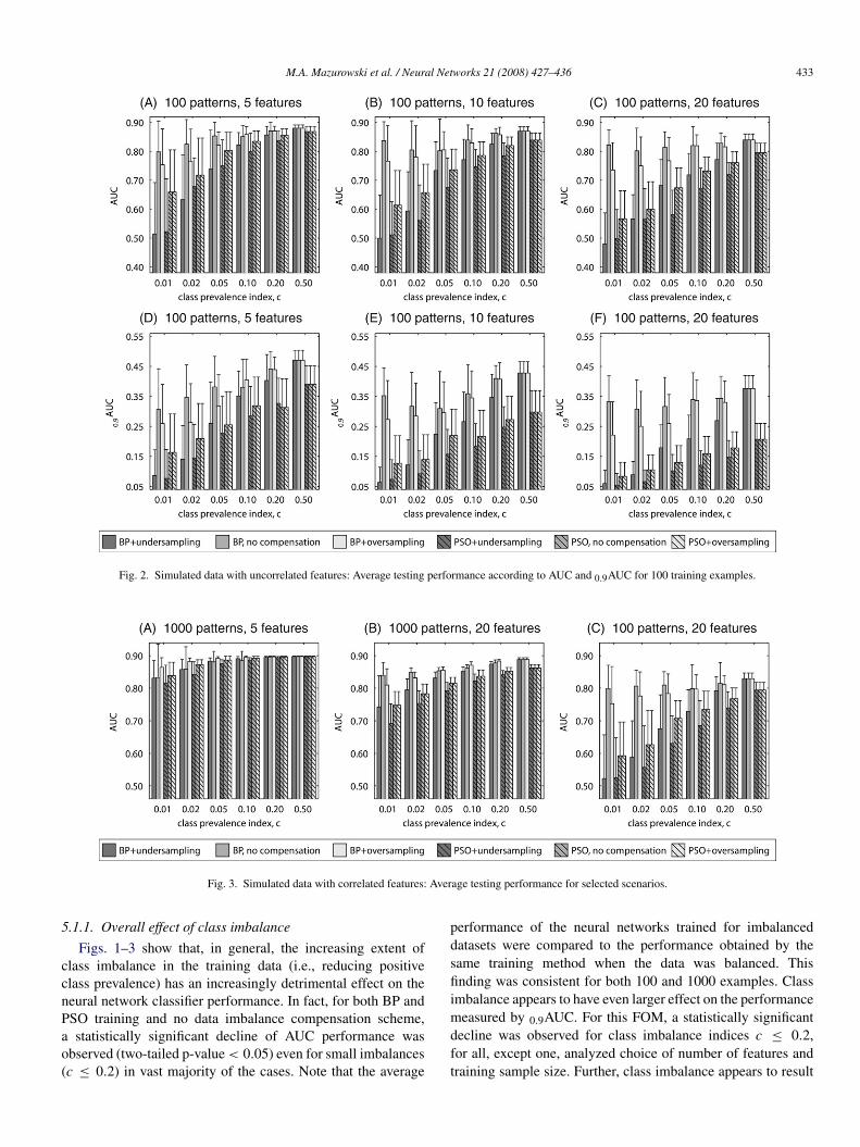
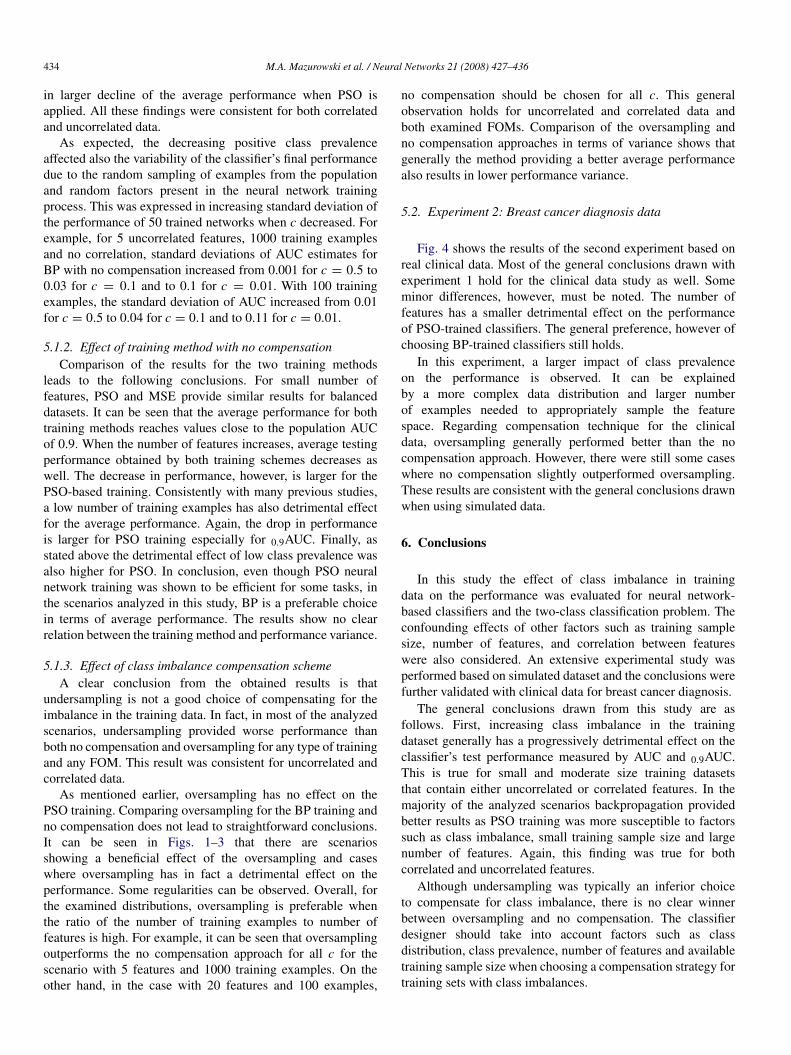
The results of Experiment 1 for uncorrelated features aresummarized in Figs. 1 and 2, each showing the neural networkaverage test performance based on the size of the trainingdataset (1000 and 100 examples, respectively). The error barsshow the standard deviations in performance obtained for 50neural networks. For each figure, there are 6 subplots. Thesubplots show average values of the two clinical FOMs (toprow — AUC, bottom row — 0.9AUC) for two different methodsof training (bars with no stripes — BP, bars with stripes —PSO) and three class imbalance handling schemes (dark grey— undersampling, medium grey — no compensation, lightgrey — oversampling). In each row, the three subplots showthe results for different number of features: 5 (subplots A andD), 10 (subplots B and E) and 20 (subplots C and F). Selectedresults for correlated features are shown in Fig. 3 to highlighttrends observed as with uncorrelated features.

M.A. Mazurowski et al. / Neural Networks 21 (2008) 427–436 433

Fig. 2. Simulated data with uncorrelated features: Average testing performance according to AUC and 0.9AUC for 100 training examples.

Fig. 3. Simulated data with correlated features: Average testing performance for selected scenarios.

5.1.1. Overall effect of class imbalance

Figs. 1–3 show that, in general, the increasing extent ofclass imbalance in the training data (i.e., reducing positiveclass prevalence) has an increasingly detrimental effect on theneural network classifier performance. In fact, for both BP andPSO training and no data imbalance compensation scheme,a statistically significant decline of AUC performance wasobserved (two-tailed p-value < 0.05) even for small imbalances(c ≤ 0.2) in vast majority of the cases. Note that the average

performance of the neural networks trained for imbalanceddatasets were compared to the performance obtained by thesame training method when the data was balanced. Thisfinding was consistent for both 100 and 1000 examples. Classimbalance appears to have even larger effect on the performancemeasured by 0.9AUC. For this FOM, a statistically significantdecline was observed for class imbalance indices c ≤ 0.2,for all, except one, analyzed choice of number of features andtraining sample size. Further, class imbalance appears to result

434 M.A. Mazurowski et al. / Neural Networks 21 (2008) 427–436

in larger decline of the average performance when PSO isapplied. All these findings were consistent for both correlatedand uncorrelated data.

As expected, the decreasing positive class prevalenceaffected also the variability of the classifier’s final performancedue to the random sampling of examples from the populationand random factors present in the neural network trainingprocess. This was expressed in increasing standard deviation ofthe performance of 50 trained networks when c decreased. Forexample, for 5 uncorrelated features, 1000 training examplesand no correlation, standard deviations of AUC estimates forBP with no compensation increased from 0.001 for c = 0.5 to0.03 for c = 0.1 and to 0.1 for c = 0.01. With 100 trainingexamples, the standard deviation of AUC increased from 0.01for c = 0.5 to 0.04 for c = 0.1 and to 0.11 for c = 0.01.

5.1.2. Effect of training method with no compensationComparison of the results for the two training methods

leads to the following conclusions. For small number offeatures, PSO and MSE provide similar results for balanceddatasets. It can be seen that the average performance for bothtraining methods reaches values close to the population AUCof 0.9. When the number of features increases, average testingperformance obtained by both training schemes decreases aswell. The decrease in performance, however, is larger for thePSO-based training. Consistently with many previous studies,a low number of training examples has also detrimental effectfor the average performance. Again, the drop in performanceis larger for PSO training especially for 0.9AUC. Finally, asstated above the detrimental effect of low class prevalence wasalso higher for PSO. In conclusion, even though PSO neuralnetwork training was shown to be efficient for some tasks, inthe scenarios analyzed in this study, BP is a preferable choicein terms of average performance. The results show no clearrelation between the training method and performance variance.

5.1.3. Effect of class imbalance compensation schemeA clear conclusion from the obtained results is that

undersampling is not a good choice of compensating for theimbalance in the training data. In fact, in most of the analyzedscenarios, undersampling provided worse performance thanboth no compensation and oversampling for any type of trainingand any FOM. This result was consistent for uncorrelated andcorrelated data.

As mentioned earlier, oversampling has no effect on thePSO training. Comparing oversampling for the BP training andno compensation does not lead to straightforward conclusions.It can be seen in Figs. 1–3 that there are scenariosshowing a beneficial effect of the oversampling and caseswhere oversampling has in fact a detrimental effect on theperformance. Some regularities can be observed. Overall, forthe examined distributions, oversampling is preferable whenthe ratio of the number of training examples to number offeatures is high. For example, it can be seen that oversamplingoutperforms the no compensation approach for all c for thescenario with 5 features and 1000 training examples. On theother hand, in the case with 20 features and 100 examples,

no compensation should be chosen for all c. This generalobservation holds for uncorrelated and correlated data andboth examined FOMs. Comparison of the oversampling andno compensation approaches in terms of variance shows thatgenerally the method providing a better average performancealso results in lower performance variance.

5.2. Experiment 2: Breast cancer diagnosis data

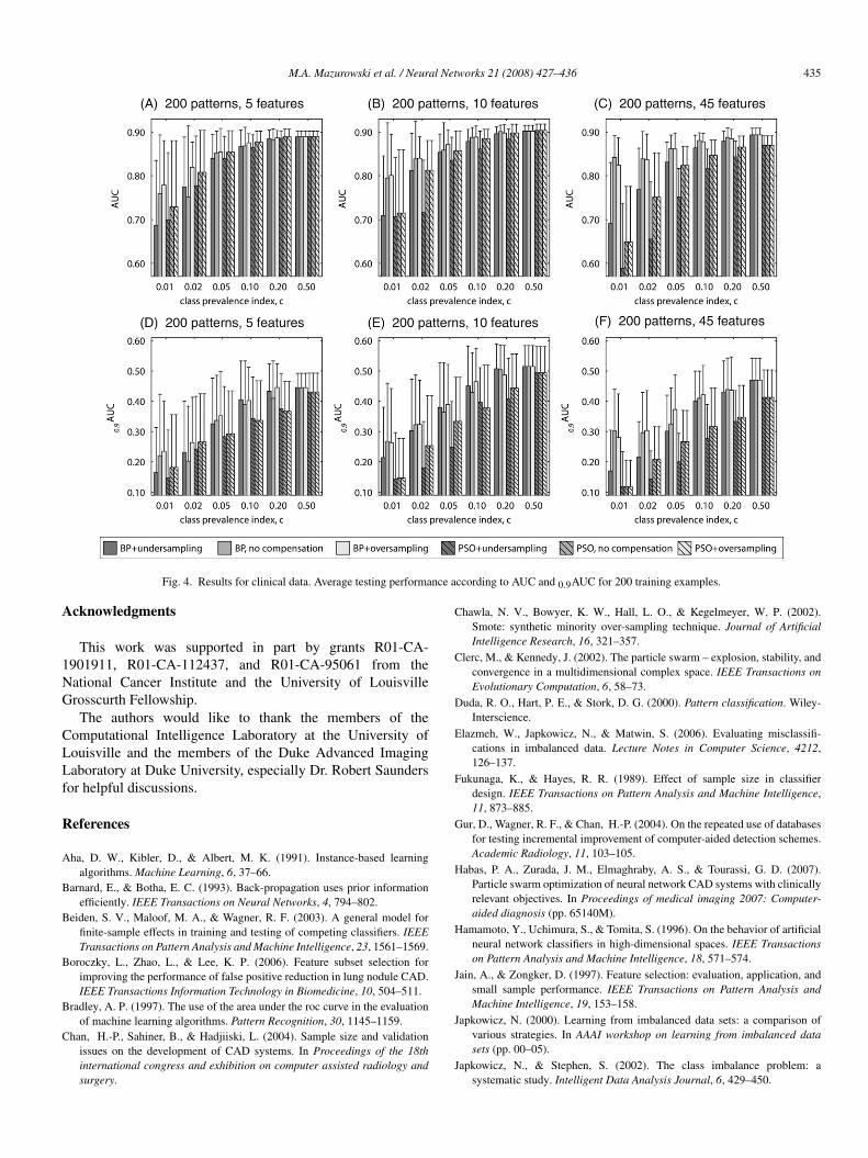
Fig. 4 shows the results of the second experiment based onreal clinical data. Most of the general conclusions drawn withexperiment 1 hold for the clinical data study as well. Someminor differences, however, must be noted. The number offeatures has a smaller detrimental effect on the performanceof PSO-trained classifiers. The general preference, however ofchoosing BP-trained classifiers still holds.

In this experiment, a larger impact of class prevalenceon the performance is observed. It can be explainedby a more complex data distribution and larger numberof examples needed to appropriately sample the featurespace. Regarding compensation technique for the clinicaldata, oversampling generally performed better than the nocompensation approach. However, there were still some caseswhere no compensation slightly outperformed oversampling.These results are consistent with the general conclusions drawnwhen using simulated data.

6. Conclusions

In this study the effect of class imbalance in trainingdata on the performance was evaluated for neural network-based classifiers and the two-class classification problem. Theconfounding effects of other factors such as training samplesize, number of features, and correlation between featureswere also considered. An extensive experimental study wasperformed based on simulated dataset and the conclusions werefurther validated with clinical data for breast cancer diagnosis.

The general conclusions drawn from this study are asfollows. First, increasing class imbalance in the trainingdataset generally has a progressively detrimental effect on theclassifier’s test performance measured by AUC and 0.9AUC.This is true for small and moderate size training datasetsthat contain either uncorrelated or correlated features. In themajority of the analyzed scenarios backpropagation providedbetter results as PSO training was more susceptible to factorssuch as class imbalance, small training sample size and largenumber of features. Again, this finding was true for bothcorrelated and uncorrelated features.

Although undersampling was typically an inferior choiceto compensate for class imbalance, there is no clear winnerbetween oversampling and no compensation. The classifierdesigner should take into account factors such as classdistribution, class prevalence, number of features and availabletraining sample size when choosing a compensation strategy fortraining sets with class imbalances.

M.A. Mazurowski et al. / Neural Networks 21 (2008) 427–436 435

Fig. 4. Results for clinical data. Average testing performance according to AUC and 0.9AUC for 200 training examples.

Acknowledgments

This work was supported in part by grants R01-CA-1901911, R01-CA-112437, and R01-CA-95061 from theNational Cancer Institute and the University of LouisvilleGrosscurth Fellowship.

The authors would like to thank the members of theComputational Intelligence Laboratory at the University ofLouisville and the members of the Duke Advanced ImagingLaboratory at Duke University, especially Dr. Robert Saundersfor helpful discussions.

References

Aha, D. W., Kibler, D., & Albert, M. K. (1991). Instance-based learningalgorithms. Machine Learning, 6, 37–66.

Barnard, E., & Botha, E. C. (1993). Back-propagation uses prior informationefficiently. IEEE Transactions on Neural Networks, 4, 794–802.

Beiden, S. V., Maloof, M. A., & Wagner, R. F. (2003). A general model forfinite-sample effects in training and testing of competing classifiers. IEEETransactions on Pattern Analysis and Machine Intelligence, 23, 1561–1569.

Boroczky, L., Zhao, L., & Lee, K. P. (2006). Feature subset selection forimproving the performance of false positive reduction in lung nodule CAD.IEEE Transactions Information Technology in Biomedicine, 10, 504–511.

Bradley, A. P. (1997). The use of the area under the roc curve in the evaluationof machine learning algorithms. Pattern Recognition, 30, 1145–1159.

Chan, H.-P., Sahiner, B., & Hadjiiski, L. (2004). Sample size and validationissues on the development of CAD systems. In Proceedings of the 18thinternational congress and exhibition on computer assisted radiology andsurgery.

Chawla, N. V., Bowyer, K. W., Hall, L. O., & Kegelmeyer, W. P. (2002).Smote: synthetic minority over-sampling technique. Journal of ArtificialIntelligence Research, 16, 321–357.

Clerc, M., & Kennedy, J. (2002). The particle swarm – explosion, stability, andconvergence in a multidimensional complex space. IEEE Transactions onEvolutionary Computation, 6, 58–73.

Duda, R. O., Hart, P. E., & Stork, D. G. (2000). Pattern classification. Wiley-Interscience.

Elazmeh, W., Japkowicz, N., & Matwin, S. (2006). Evaluating misclassifi-cations in imbalanced data. Lecture Notes in Computer Science, 4212,126–137.

Fukunaga, K., & Hayes, R. R. (1989). Effect of sample size in classifierdesign. IEEE Transactions on Pattern Analysis and Machine Intelligence,11, 873–885.

Gur, D., Wagner, R. F., & Chan, H.-P. (2004). On the repeated use of databasesfor testing incremental improvement of computer-aided detection schemes.Academic Radiology, 11, 103–105.

Habas, P. A., Zurada, J. M., Elmaghraby, A. S., & Tourassi, G. D. (2007).Particle swarm optimization of neural network CAD systems with clinicallyrelevant objectives. In Proceedings of medical imaging 2007: Computer-aided diagnosis (pp. 65140M).

Hamamoto, Y., Uchimura, S., & Tomita, S. (1996). On the behavior of artificialneural network classifiers in high-dimensional spaces. IEEE Transactionson Pattern Analysis and Machine Intelligence, 18, 571–574.

Jain, A., & Zongker, D. (1997). Feature selection: evaluation, application, andsmall sample performance. IEEE Transactions on Pattern Analysis andMachine Intelligence, 19, 153–158.

Japkowicz, N. (2000). Learning from imbalanced data sets: a comparison ofvarious strategies. In AAAI workshop on learning from imbalanced datasets (pp. 00–05).

Japkowicz, N., & Stephen, S. (2002). The class imbalance problem: asystematic study. Intelligent Data Analysis Journal, 6, 429–450.

436 M.A. Mazurowski et al. / Neural Networks 21 (2008) 427–436

Jesneck, J. L., Lo, J. Y., & Baker, J. A. (2007). Breast mass lesions: computer-aided diagnosis models with mammographic and sonographic descriptors.Radiology, 244, 390–398.

Jiang, Y., Metz, C. E., & Nishikawa, R. M. (1996). A receiver operatingcharacteristic partial area index for highly sensitive diagnostic tests.Radiology, 201, 745–750.

Kawamoto, K., Houlihan, C. A., Balas, E. A., & Lobach, D. F. (2005).Improving clinical practice using clinical decision support systems: asystematic review of trials to identify features critical to success. BritishMedical Journal, 330, 765–772.

Kennedy, J., & Eberhart, R. (1995). Particle swarm optimization. InProceedings of IEEE international conference on neural networks (pp.1942–1948).

Li, Q., & Doi, K. (2006). Reduction of bias and variance for evaluation ofcomputer-aided diagnostic schemes. Medical Physics, 33, 868–875.

Li, Q., & Doi, K. (2007). Comparison of typical evaluation methodsfor computer-aided diagnostic schemes: Monte Carlo simulation study.Medical Physics, 34, 871–876.

Lisboa, P. J. (2002). A review of evidence of health benefit from artificial neuralnetworks in medical intervention. Neural Networks, 15, 11–39.

Lisboa, P. J., & Taktak, A. F. G. (2006). The use of artificial neural networksin decision support in cancer: a systematic review. Neural Networks, 19,408–415.

Maloof, M. A. (2003). Learning when data sets are imbalanced and when costsare unequal and unknown. In Proceedings of workshop on learning fromimbalanced data sets.

Mazurowski, M. A., Habas, P. A., Zurada, J. M., & Tourassi, G. D. (2007).Impact of low class prevalence on the performance evaluation of neuralnetwork based classifiers: Experimental study in the context of computer-assisted medical diagnosis. In Proceedings of international joint conferenceon neural networks (pp. 2005–2009).

Metz, C. E., Herman, B. A., & Shen, J.-H. (1998). Maximum likelihoodestimation of receiver operating characteristic (ROC) curves fromcontinuously-distributed data. Statistics in Medicine, 17, 1033–1053.

Mitchell, T. (1997). Machine learning. McGraw Hill.

Obuchowski, N. A. (2003). Receiver operating characteristic curves and theiruse in radiology. Radiology, 229, 3–8.

Raudys, S. (1997). On dimensionality, sample size, and classification errorof nonparametric linear classification algorithms. IEEE Transactions onPattern Analysis and Machine Intelligence, 19, 667–671.

Raudys, S. J., & Jain, A. K. (1991). Small sample size effects in statisticalpattern recognition: recommendations for practitioners. IEEE Transactionson Pattern Analysis and Machine Intelligence, 13, 252–264.

Rumelhart, D. E., Hinton, G. E., & Williams, R. J. (1986). Learning internalrepresentations by error propagation. In Parallel distributed processing:Explorations in the microstructure of cognition, volume 1 (pp. 318–362).MIT Press.

Sahiner, B., Chan, H. P., Petrick, N., Wagner, R. F., & Hadjiiski, L. (2000).Feature selection and classifier performance in computer-aided diagnosis:the effect of finite sample size. Medical Physics, 27, 1509–1522.

Sampat, M. P., Markey, M. K., & Bovik, A. C. (2005). Computer-aideddetection and diagnosis in mammography. In Handbook of image and videoprocessing (pp. 1195–1217). Academic Press.

van den Bergh, F., & Engelbrecht, A. P. (2004). A cooperative approachto particle swarm optimization. IEEE Transactions on EvolutionaryComputation, 8, 225–239.

Wagner, R. F., Chan, H.-P., Sahiner, B., & Petrick, N. (1997). Finite-sample effects and resampling plans: applications to linear classifiers incomputer-aided diagnosis. In Proceedings of medical imaging 1997: Imageprocessing (pp. 467–477).

Weiss, G. M., & Provost, F. (2001). The effect of class distribution on classifierlearning: an empirical study. Technical report, Department of ComputerScience, Rutgers University.

Zhang, G. P. (2000). Neural networks for classification: a survey. IEEETransactions on Systems, Man, and Cybernetics – Part C: Applications andReviews, 30, 451–462.

Zhou, Z.-H., & Liu, X.-Y. (2006). Training cost-sensitive neural networkswith methods addressing the class imbalance problem. IEEE Transactionson Knowledge and Data Engineering, 18, 63–77.