Trajectory Design and Control for Formation Flying Spaceborne Interferometers by Christophe Ph. Mandy Lic. Sc. Math., ULB (2006) Submitted to the Department of Aeronautics and Astronautics in partial fulfillment of the requirements for the degree of Masters of Science in Aeronautics and Astronautics at the MASSACHUSETTS INSTITUTE OF TECHNOLOGY June 2009 c Massachusetts Institute of Technology 2009. All rights reserved. Author .............................................................. Department of Aeronautics and Astronautics May 27th, 2009 Certified by .......................................................... David W. Miller Professor Thesis Supervisor Accepted by ......................................................... David L. Darmofal Associate Department Head Chair, Committee on Graduate Students
Transcript
Trajectory Design and Control for Formation
Flying Spaceborne Interferometers
by
Christophe Ph. Mandy
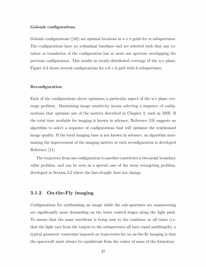
Lic. Sc. Math., ULB (2006)
Submitted to the Department of Aeronautics and Astronauticsin partial fulfillment of the requirements for the degree of
Masters of Science in Aeronautics and Astronautics
Associate Department HeadChair, Committee on Graduate Students
2
Trajectory Design and Control for Formation Flying
Spaceborne Interferometers
by
Christophe Ph. Mandy
Submitted to the Department of Aeronautics and Astronauticson May 27th, 2009, in partial fulfillment of the
requirements for the degree ofMasters of Science in Aeronautics and Astronautics
Abstract
Spaceborne interferometry promises to greatly expand our knowledge of astronomyand astrophysics, and open the doors to many new discoveries. The purpose of thisstudy is to investigate optimal resource management techniques for separated space-craft interferometers to successfully synthesize images. Assuming optimal imagingconfigurations that satisfy astronomical requirements have been selected, a two-stepapproach is taken to satisfy these requirements: (1) develop a framework to man-age control effort among different satellites during observation and retargeting of thespacecraft formations, to thereby maximize the number of observations that can betaken with a given amount of consumables, and (2) determine computationally ef-ficient control techniques to minimize control effort while meeting image synthesismetrics. First, issues relating to planning optimal trajectories that trade imagingmetrics for spacecraft design metrics such as mission length and spacecraft massare addressed. The determination of optimal spacecraft locations or trajectories forimage acquisition is studied to satisfy astronomical constraints. These positioningrequirements lead to the computation of trajectories for the retargeting of formationflying interferometers to capture images of a new astronomical target. Second, thetrajectories planned under this appraoch are used in the formulation of a trackingcontrol problem for spaceborne interferometric apertures. The assumptions madein the control problem are used as a basis for the development of different controltechniques that trade image quality for fuel expenditure, and evaluated according toscenarios involving different properties relevant to synthetic imaging. The result fromthese two steps are then applied to the SPHERES testbed, a six-degree-of-freedomfacility designed for the incremental maturation of formation flight technologies in arisk-tolerant microgravity environment. Results from simulations and experiments onboard the space station are presented and compared to their theoretical outcomes.
Thesis Supervisor: David W. MillerTitle: Professor
3
4
Acknowledgments
There are many people I must recognize for their invaluable help and support during
the completion of the research presented in this thesis. I have been very lucky to
work in close contact with an amazing team of researchers and staff in the Space
Systems Laboratory. In particular, I’d like to thank Dr. Soon-Jo Chung, for inspiring
me to set high standards in my work; Dr. Hiraku Sakamoto, for teaching me to be
inquisitive and disciplined; Dr. Simon Nolet, for showing me the value of perseverance;
and especially Dr. Alvar Saenz-Otero, for leading by example and inspiring me to
work thoroughly. I’d also like to express my appreciation to my office mates: Mark
Baldesarra, Nick Hoff, Christy Edwards and Swati Mohan, for their friendliness and
support.
I must next acknowledge my many friends who supported me during my master’s
program and greatly enriched my life, particularly Rhea Patricia Liem, Adrienne Li
and Sonja Wogrin. I would also like to thank my parents, for their unwavering support
and for opening so many possibilities for me.
Finally, I’d like to express my deepest gratitude to my advisor, Professor David
Miller. I am forever indebted for the incomparable opportunities that he made avail-
able to me, for trusting me with exciting and invaluable projects, for his counsel,
generosity and inexhaustible patience. I have had a very enjoyable and life-changing
3 years at MIT, in no small part thanks to him.
5
6
Contents
1 Introduction 17
1.1 The need for spaceborne interferometers . . . . . . . . . . . . . . . . 18
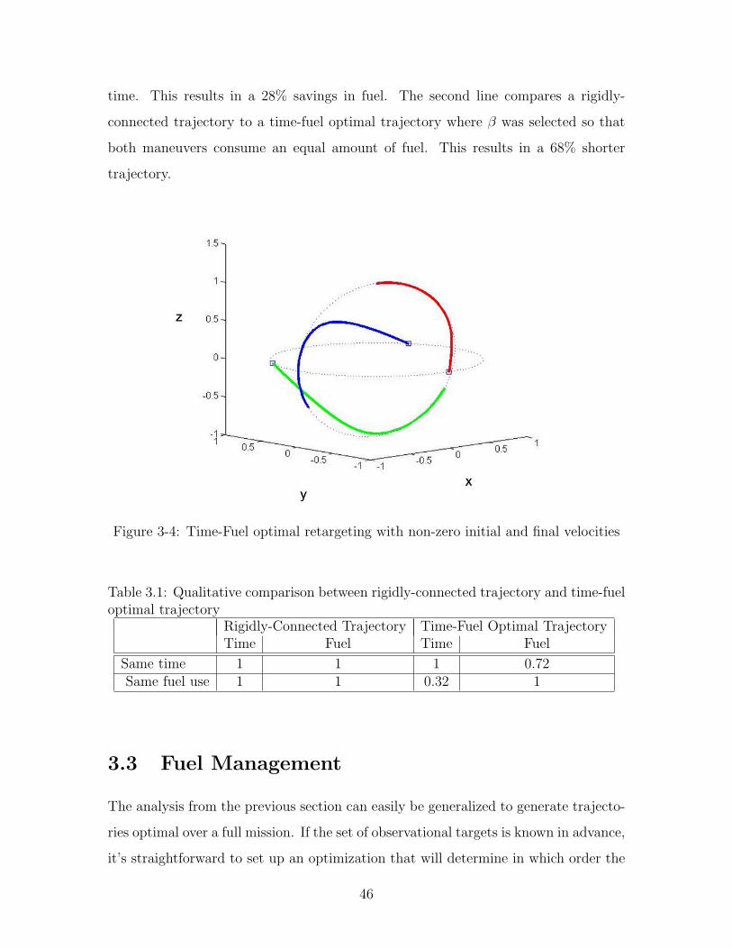
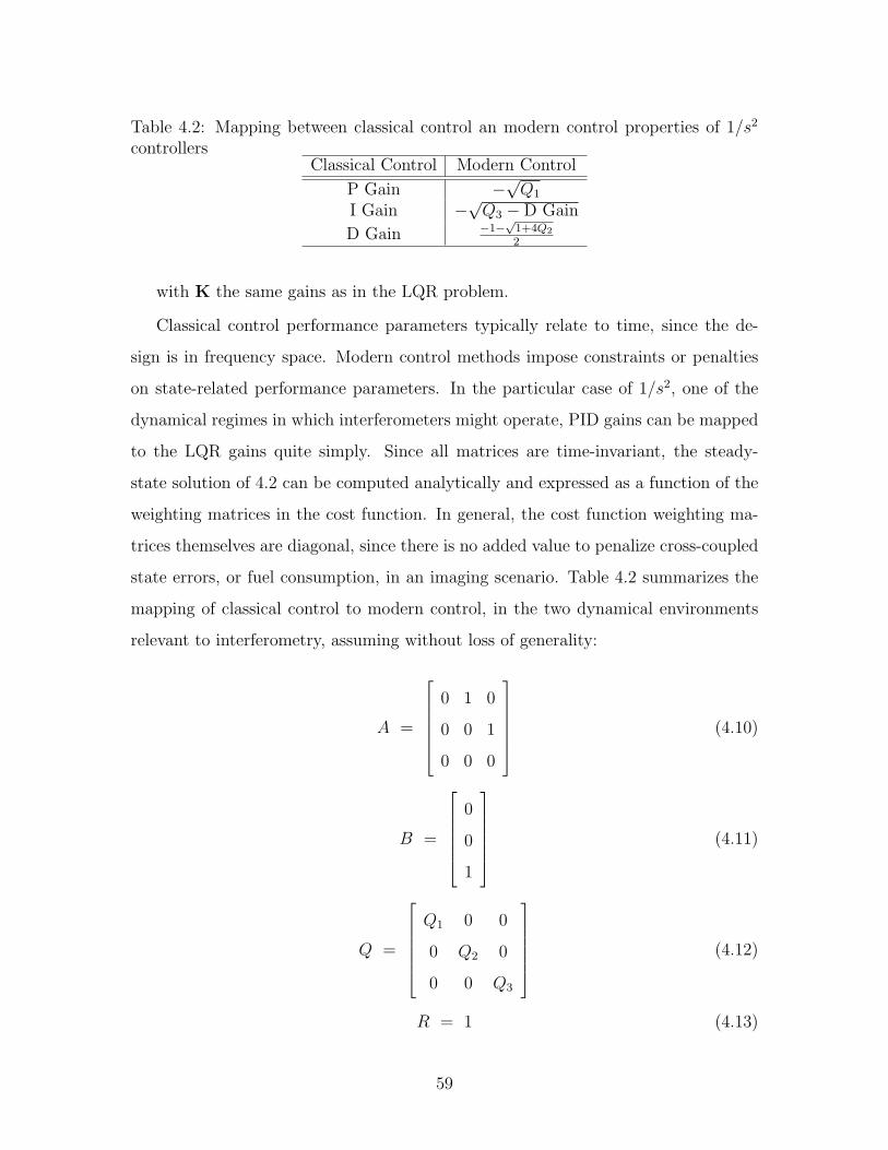
penalty term or the control penalty term in the cost fucntion. The gains for each
controller in Figure 4-3, Figure 4-4 and Figure 4-5 were selected to meet the same
mean-squared error performance as in Figure 4-2. The performance of these four
controllers is summarized in table 4.3.
The actual performance of the controller depends on the specific gains used. To
illustrate the possible spread of performances, the plots on the right of the Figures
shows the possible performance values attainable with the controller: the horizon-
tal axis corresponds to ∆v, the vertical axis to mean-squared error and coordinate
points are plotted for different gain settings. These are the plots that give a sense
of the potential value of any controller. Any single mission can be viewed from two
perspectives: astronomers suggest a desired imaging quality, which translates into a
mean-squared-error requirement, and the controller should try to meet the require-
ment with as little fuel as possible. Alternatively, the array is in space and has a
61
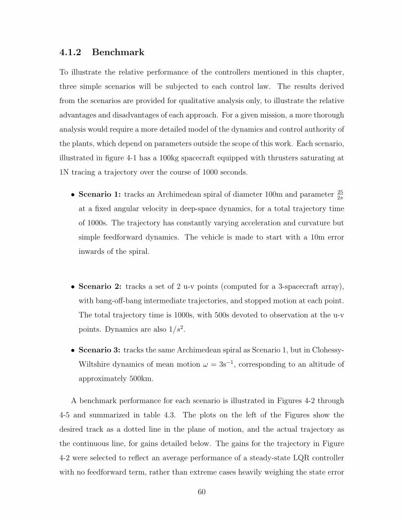
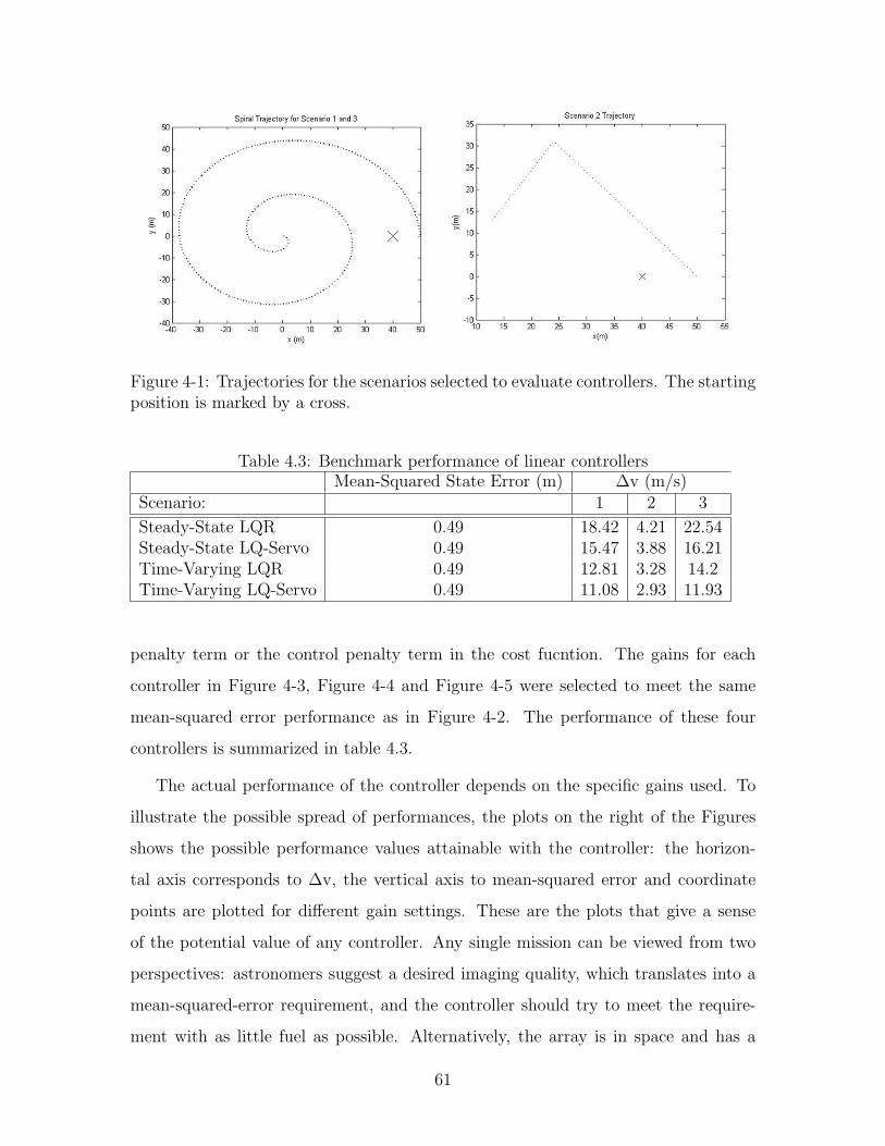
Figure 4-2: Steady-state LQR controller with no feedforward component performancefor each scenario
62
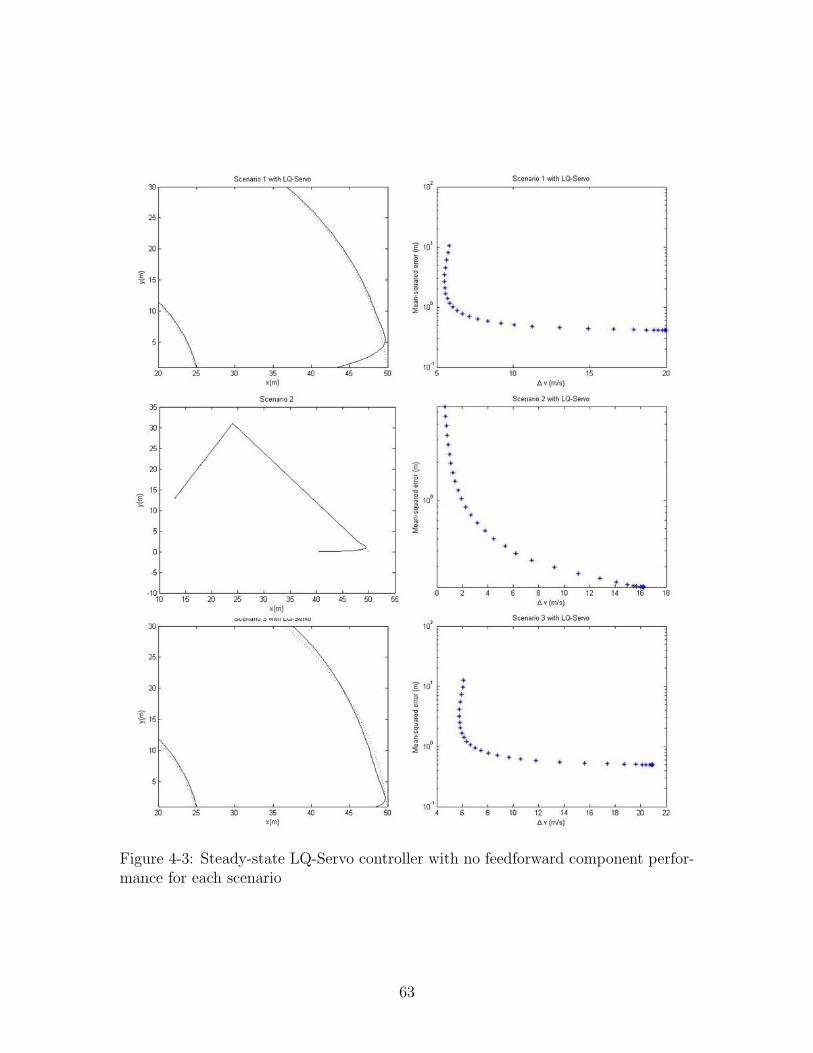
Figure 4-3: Steady-state LQ-Servo controller with no feedforward component perfor-mance for each scenario
63
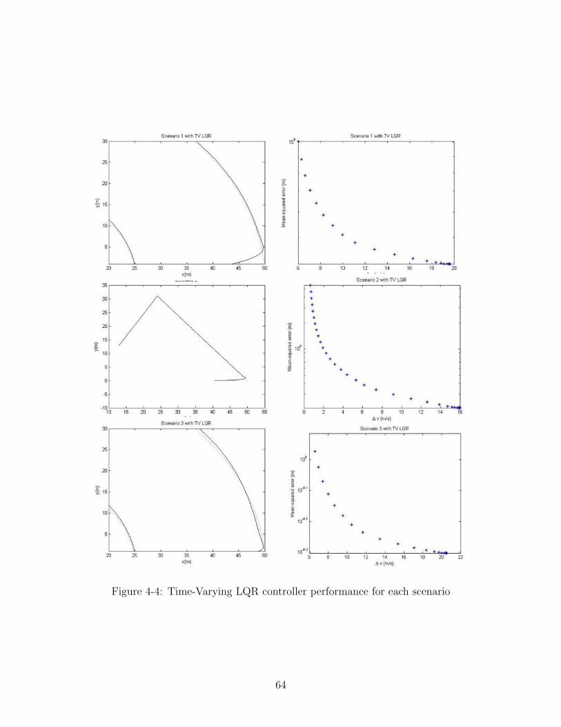
Figure 4-4: Time-Varying LQR controller performance for each scenario
64
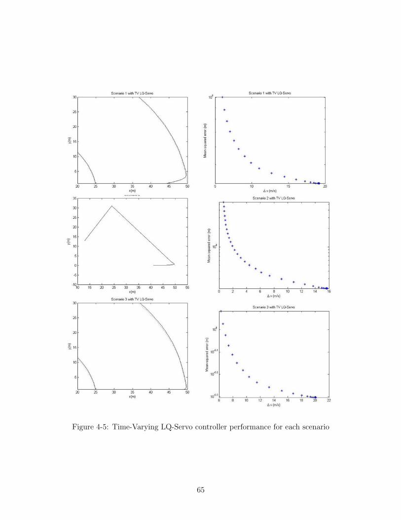
Figure 4-5: Time-Varying LQ-Servo controller performance for each scenario
65
limited supply of fuel. Given a set of possible imaging targets, the controller should
try to minimize mean-squared-error of each image according to how much ∆v is allo-
cated to each image. Finding which controller to use corresponds to seeking on such
a figure the desired mean-squared error or ∆v and finding the smallest associated
value of the other metric.
Figure 4-2 shows the performance of a steady-state LQR controller. Since there is
no particular reason to weigh any state more heavily than any other in the scenarios,
or to cross-weigh any two states or control commands, the matrices in 4.2 were selected
to be diagonal:
Hf = 0
wxQ =
1 0 0 0
0 1 0 0
0 0 1 0
0 0 0 1
wuR =
1 0
0 1
(4.14)
with wx = 1 and wu = 104. The right plot in the figure was obtained by varying the
ratio wx
wu.
Figure 4-3 shows the performance of a steady-state LQ-Servo controller. In this
case, the dynamics are extended as in equation 4.8, and the cost function matrices
are again diagonal:
Hf = 0
wxQ = I8×8
wuR = I2×2
(4.15)
with wx = 1 and wu = 3678 to match the mean-squared error from figure 4-2. The
right plot in the figure was again obtained by varying the ratio wx
wu.
Figure 4-4 shows the performance of a time-varying LQR controller, where the
gains are obtained by solving equations 4.5 and 4.6. In this case, the final state error
66
must be penalized as well, and the matrices were:
Hf = wxQ = I4×4
wuR = I2×2
(4.16)
with wx = 1.45 and wu = 1244 to match the mean-squared error from figure 4-2. The
right plot in the figure was again obtained by varying the values of wx and wu.
Finally, Figure 4-5 shows the performance of a time-varying LQ-Servo controller,
with cost function matrices:
Hf = wxQ = I8×8
wuR = I2×2
(4.17)
with wx = 1.62 and wu = 982 to match the mean-squared error from figure 4-2. The
right plot in the figure was again obtained by varying the values of wx and wu.
The drop in fuel use for any given mean-squared error when comparing the steady-
state cases to the time-varying cases shows the value in using time-varying gains.
These capture both the required feedforward component (calculated from equation
4.6) as well as the non-uniform nature of a linear-quadratic optimization problem
expressed with a quadratic cost function. As the trajectory nears its end, the feedback
term in the controllers will drive the error down. Similarly, the effect of augmenting
the dynamics from the LQR formulation to the LQ-Servo formulation reduces teh
mean-squared error by imposing further constraints on the state error over the course
of the trajectory.
4.2 Discretization
It is in general not possible to instantaneously and continuously control dynamical
systems. Time delays stemming from data transfer and computation result in various
lags in the system, so that the system is better modeled as a discrete mathemati-
cal process. Since the underlying dynamics of formation flying interferometers are
continuous, the most common approach to control design is emulation: designing a
67
continuous compensator, for instance PID or LQ-Servo, digitizing the dynamics and
tweaking the results to improve performance, based on a simulation or hardware data.
The more computationally costly approach is to simply solve discrete variational
problem, expressing a cost function, control and dynamics in discrete terms and
implementing the resulting optimal control law.
For this section, a slight modification done to scenarios: the geometric trajectory
characteristics are maintained, but a digitization period of 1 is enforced so that the
trajectory becomes a sequence of step inputs. In the context of the imaging scenarios,
only the aperture’s locations matter, but it can be shown ([13]) that the optimal
reference velocity at each discretized point is the same as the velocity (and further
time derivatives) the craft would have if it were to follow the continuous trajectory.
4.2.1 Discrete LQ-Servo
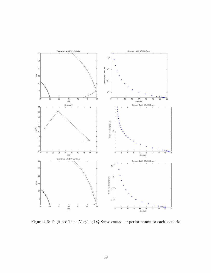
Figure 4-6 shows the performance of a digitized time-varying LQ-Servo controller with
a continuous cost function defined by the weighting matrices in equation 4.17. The
values of wx = 1.62 and wu = 1128 were selected to match the mean-squared error
from Figure 4-2. The right plots in Figure 4-6 show the spread of possible metric
values as wx and wu are varied. The digitization imposes a small discretization error
which reduces the performance of the controller compared to its continuous version
in 4-5.
4.2.2 Timestepped Bang-Off-Bang actuation
Invariably, digitization makes an assumption on control: that at any discrete control
period, only one command is given to the actuators. Since all relevant dynamics
are linear, the discretized command is also assumed to be linear. But this does
not necessarily have to be the case, particularly since there are no linear continuous
actuators for spacecraft positioning. Although it may not be computationally feasible
to compute an actual optimal path at each step, another simple fuel-saving technique
is possible. At each timestep, initial conditions (at time t0) are known, and a final
68
Figure 4-6: Digitized Time-Varying LQ-Servo controller performance for each scenario
69
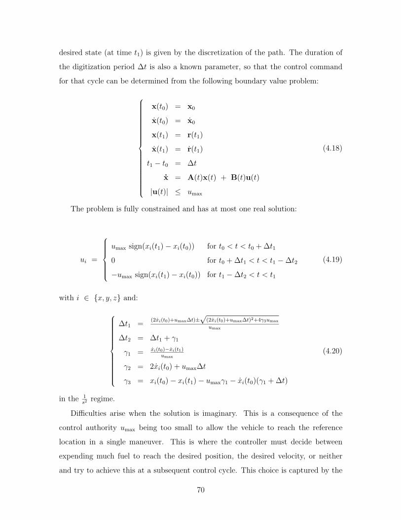
desired state (at time t1) is given by the discretization of the path. The duration of
the digitization period ∆t is also a known parameter, so that the control command
for that cycle can be determined from the following boundary value problem:
x(t0) = x0
x(t0) = x0
x(t1) = r(t1)
x(t1) = r(t1)
t1 − t0 = ∆t
x = A(t)x(t) + B(t)u(t)
|u(t)| ≤ umax
(4.18)
The problem is fully constrained and has at most one real solution:
ui =
umax sign(xi(t1)− xi(t0)) for t0 < t < t0 + ∆t1
0 for t0 + ∆t1 < t < t1 −∆t2
−umax sign(xi(t1)− xi(t0)) for t1 −∆t2 < t < t1
(4.19)
with i ∈ {x, y, z} and:
∆t1 =(2xi(t0)+umax∆t)±
√(2xi(t0)+umax∆t)2+4γ3umax
umax
∆t2 = ∆t1 + γ1
γ1 = xi(t0)−xi(t1)umax
γ2 = 2xi(t0) + umax∆t
γ3 = xi(t0)− xi(t1)− umaxγ1 − xi(t0)(γ1 + ∆t)
(4.20)
in the 1s2 regime.
Difficulties arise when the solution is imaginary. This is a consequence of the
control authority umax being too small to allow the vehicle to reach the reference
location in a single maneuver. This is where the controller must decide between
expending much fuel to reach the desired position, the desired velocity, or neither
and try to achieve this at a subsequent control cycle. This choice is captured by the
70
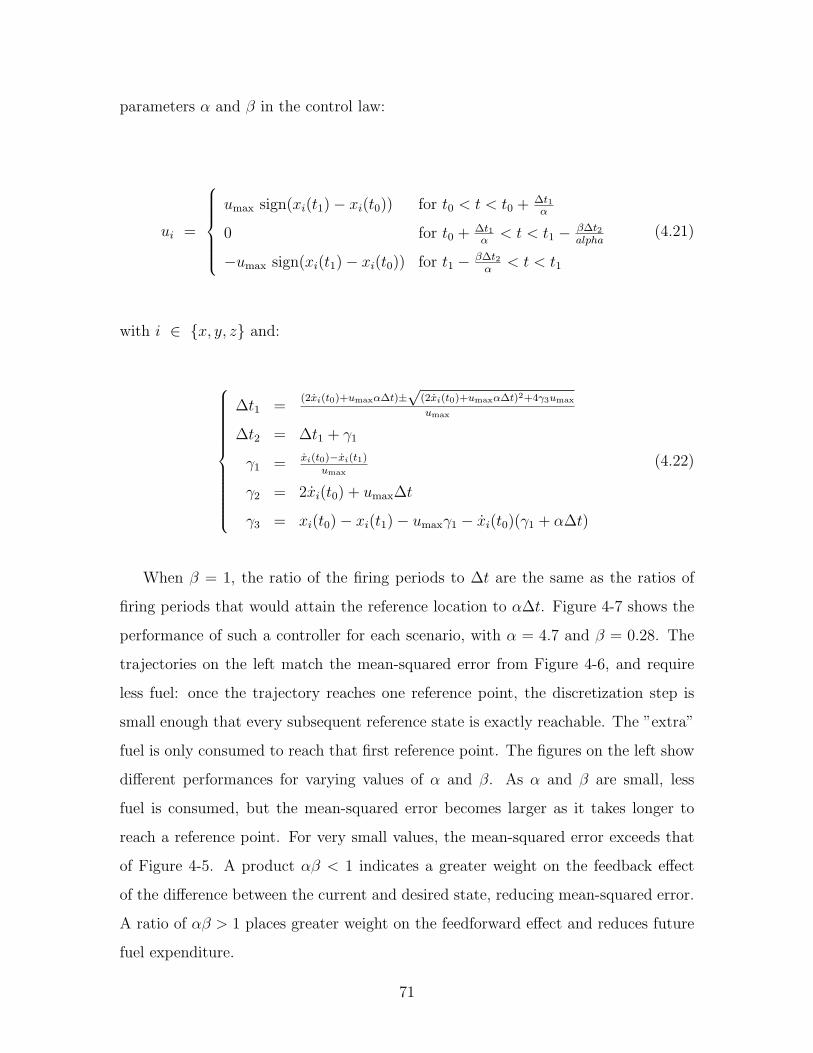
parameters α and β in the control law:
ui =
umax sign(xi(t1)− xi(t0)) for t0 < t < t0 + ∆t1
α
0 for t0 + ∆t1α
< t < t1 − β∆t2alpha
−umax sign(xi(t1)− xi(t0)) for t1 − β∆t2α
< t < t1
(4.21)
with i ∈ {x, y, z} and:
∆t1 =(2xi(t0)+umaxα∆t)±
√(2xi(t0)+umaxα∆t)2+4γ3umax
umax
∆t2 = ∆t1 + γ1
γ1 = xi(t0)−xi(t1)umax
γ2 = 2xi(t0) + umax∆t
γ3 = xi(t0)− xi(t1)− umaxγ1 − xi(t0)(γ1 + α∆t)
(4.22)
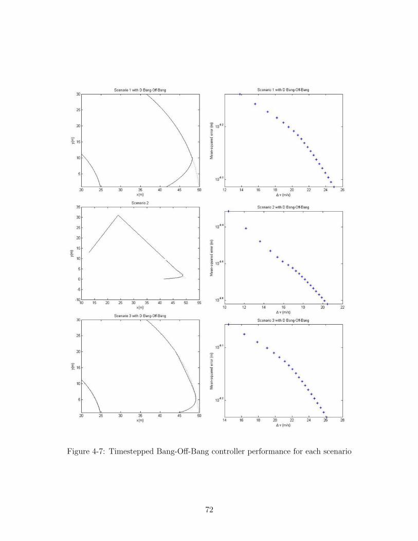
When β = 1, the ratio of the firing periods to ∆t are the same as the ratios of
firing periods that would attain the reference location to α∆t. Figure 4-7 shows the
performance of such a controller for each scenario, with α = 4.7 and β = 0.28. The
trajectories on the left match the mean-squared error from Figure 4-6, and require
less fuel: once the trajectory reaches one reference point, the discretization step is
small enough that every subsequent reference state is exactly reachable. The ”extra”
fuel is only consumed to reach that first reference point. The figures on the left show
different performances for varying values of α and β. As α and β are small, less
fuel is consumed, but the mean-squared error becomes larger as it takes longer to
reach a reference point. For very small values, the mean-squared error exceeds that
of Figure 4-5. A product αβ < 1 indicates a greater weight on the feedback effect
of the difference between the current and desired state, reducing mean-squared error.
A ratio of αβ > 1 places greater weight on the feedforward effect and reduces future
fuel expenditure.
71
Figure 4-7: Timestepped Bang-Off-Bang controller performance for each scenario
72
4.3 Anticipatory Tracking Control
Optimal trajectories, as defined and generated in chapter 3 are optimal in the sense
that they minimize a performance metric over the course of a trajectory. Solving
a minimization problem leads to a control output sequence that could be seen as
sequence of open-loop commands which only depend on time (u∗(t)), which would
generate optimal tracking if no disturbances perturb the system. However in solving
the minimization problem, the control is typically expressed as a function of the
system’s measured state or state error, and applying Pontryagin’s minimum principle,
substituted in a system of Lagrange-Hamilton equations to find the the trajectory that
minimizes the performance metric (x∗(t)). This optimal trajectory is then replaced in
the expression of the optimal control, to determine what the required control output
should be (u∗(x∗(t), t)). This is precisely what is done in section 4.1 to solve the
LQR tracking problem. In the vast majority of cases treated in the literature, the
optimal control is only implicitly dependent on time through the optimal trajectory
(u∗(x∗(t))). A common paradigm is to then use this control law to track the desired
trajectory, but having the optimal trajectory as a reference input, and determining
the control based on the actual state (x(t)). But the resulting control sequence
(u(x(t), t)) is not necessarily optimal anymore: as perturbations push the system off
the desired track, the ideal controller would re-solve the optimization problem online
and re-determine an optimal trajectory. This has two drawbacks: it is often very
difficult to prove that the system will converge over repeated optimizations, and it is
generally not computationally possible to solve the minimization problem repeatedly.
The convenience of substituting the actual state into the control logic results
in controllers that aren’t optimal in the minimization sense, but that have tuning
parameters that can be adjusted to try to achieve best performance. And these very
often don’t perform well in nonlinear dynamical cases, where the state error can
actually expand when following such a control logic, leading to nonlinear controllers
that appear to perform significantly better than the classical paradigm.
In the tracking problem for Interferometric Arrays, one crucial piece of information
73
is lost when following this paradigm, and often when implementing a more advanced
nonlinear tracking controller: the future track is known, and not just limited to a
single state-space location at a single point in time. When the minimization problem
is solved with variational methods, the solution is optimal because it ”anticipates”
the future states of the system and determines the optimal control command now,
to take these future states into account (in most cases, this is achieved by backwards
integration). But when substituting the current state or state error in the control law,
the control gains don’t multiply the state in a way that anticipates future accelera-
tions, velocities and state errors, leading to avoidable overshooting or lags. There are
three ways to take this extra information into account, which will be explored here:
the reference input can be selected to be a state-space location at a point a (possibly
variable) amount of time in the future, where this time interval functions as a gain;
the reference input can take into account all the time-derivatives of the trajectory at
the reference time; and the reference input can be chosen to be a set of integrals of
the trajectory over a moving window of time in the future.
4.3.1 The Park Controller
In [26], Park et al. propose a very simple nonlinear guidance logic for UAVs that
outperforms PD and PID controllers for curved trajectories, particularly circles. Ref-
erences [27] and [10] further elaborate on the stability and performance of the logic.
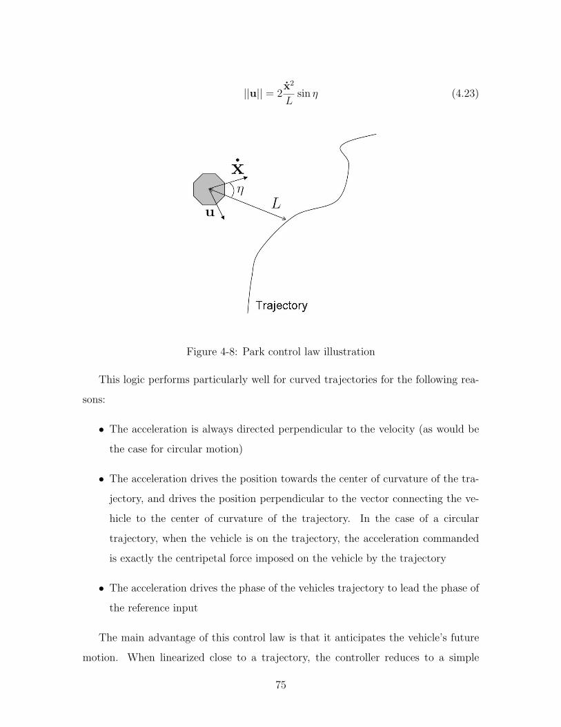
The logic is as follows2: at each timestep, a reference point is selected on the track,
at a fixed distance L from the system (if L is small enough compared to trajectory,
there will in general be two such points, and the forward point is selected as the
reference point). The acceleration commanded by the system is then chosen to be
the instantaneous centripetal acceleration necessary to follow a circular arc from the
current state to the reference point, of radius L2 sin η
(see figure 4-8).
2The logic was developed for 2-dimensional trajectories and motion, but is readily generalizableto three dimensions: the two-dimensional results are applicable to the plane defined by the velocityvector and the reference point
74
||u|| = 2x2
Lsin η (4.23)
Figure 4-8: Park control law illustration
This logic performs particularly well for curved trajectories for the following rea-
sons:
• The acceleration is always directed perpendicular to the velocity (as would be
the case for circular motion)
• The acceleration drives the position towards the center of curvature of the tra-
jectory, and drives the position perpendicular to the vector connecting the ve-
hicle to the center of curvature of the trajectory. In the case of a circular
trajectory, when the vehicle is on the trajectory, the acceleration commanded
is exactly the centripetal force imposed on the vehicle by the trajectory
• The acceleration drives the phase of the vehicles trajectory to lead the phase of
the reference input
The main advantage of this control law is that it anticipates the vehicle’s future
motion. When linearized close to a trajectory, the controller reduces to a simple
75
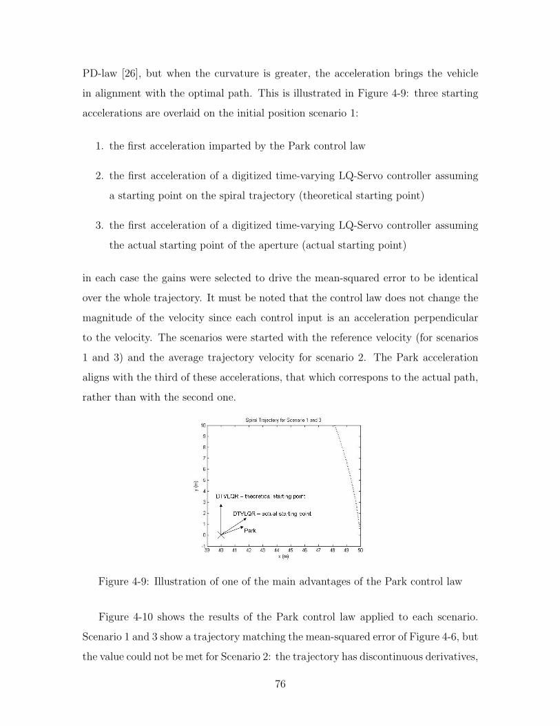
PD-law [26], but when the curvature is greater, the acceleration brings the vehicle
in alignment with the optimal path. This is illustrated in Figure 4-9: three starting
accelerations are overlaid on the initial position scenario 1:
1. the first acceleration imparted by the Park control law
2. the first acceleration of a digitized time-varying LQ-Servo controller assuming
a starting point on the spiral trajectory (theoretical starting point)
3. the first acceleration of a digitized time-varying LQ-Servo controller assuming
the actual starting point of the aperture (actual starting point)
in each case the gains were selected to drive the mean-squared error to be identical
over the whole trajectory. It must be noted that the control law does not change the
magnitude of the velocity since each control input is an acceleration perpendicular
to the velocity. The scenarios were started with the reference velocity (for scenarios
1 and 3) and the average trajectory velocity for scenario 2. The Park acceleration
aligns with the third of these accelerations, that which correspons to the actual path,
rather than with the second one.
Figure 4-9: Illustration of one of the main advantages of the Park control law
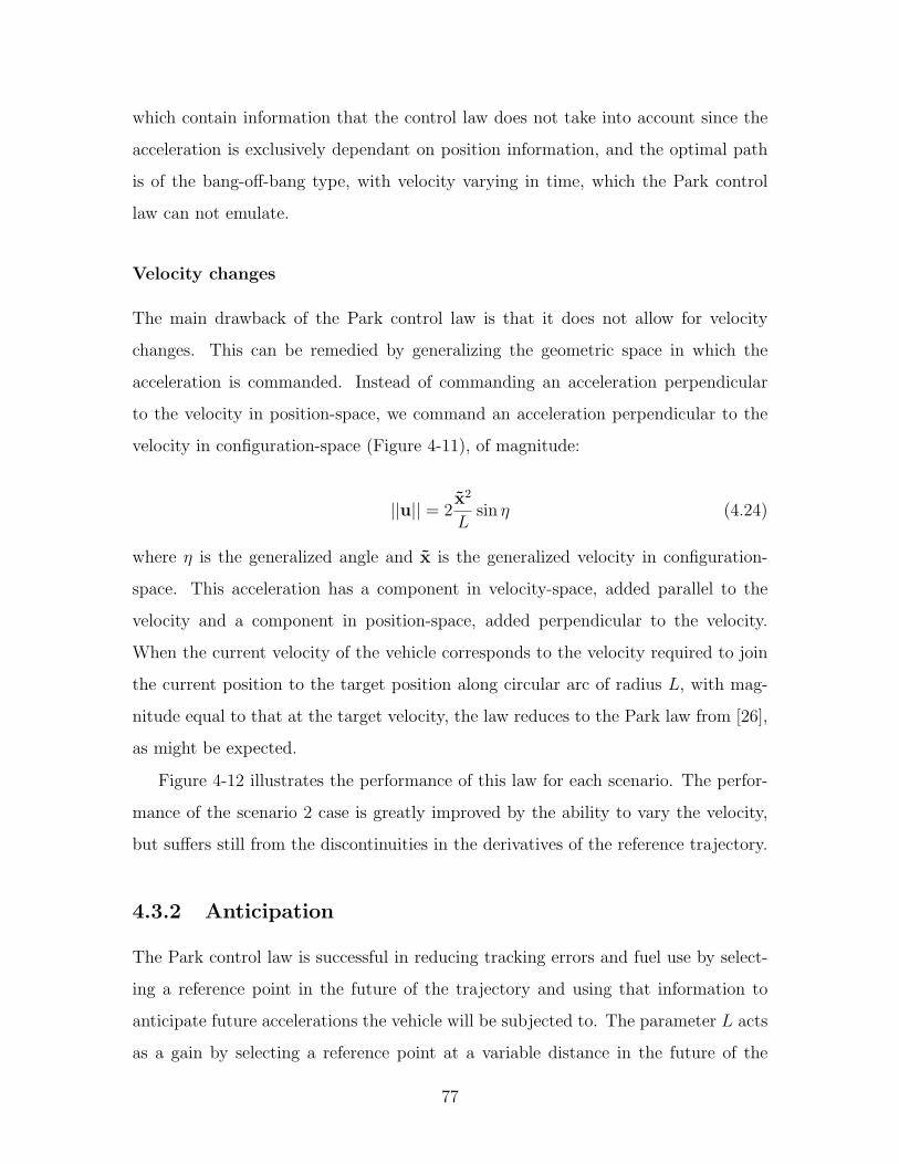
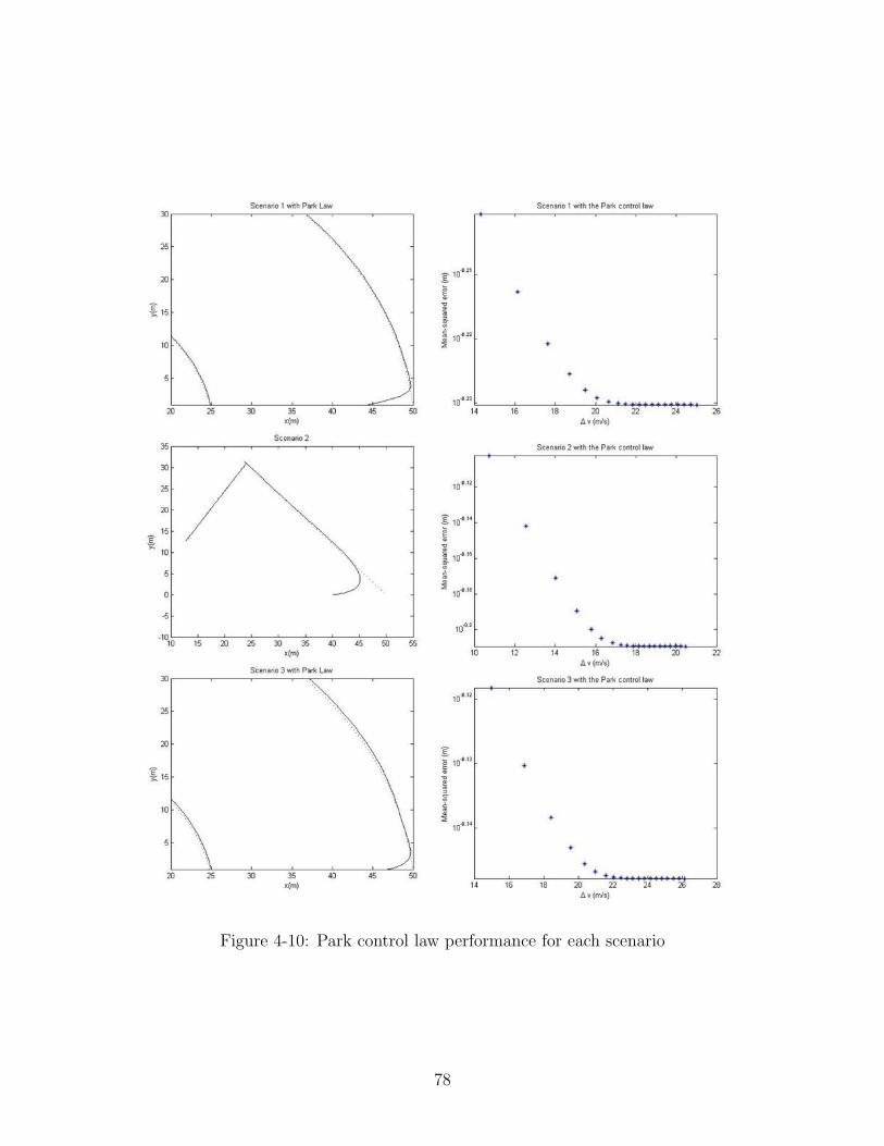
Figure 4-10 shows the results of the Park control law applied to each scenario.
Scenario 1 and 3 show a trajectory matching the mean-squared error of Figure 4-6, but
the value could not be met for Scenario 2: the trajectory has discontinuous derivatives,
76
which contain information that the control law does not take into account since the
acceleration is exclusively dependant on position information, and the optimal path
is of the bang-off-bang type, with velocity varying in time, which the Park control
law can not emulate.
Velocity changes
The main drawback of the Park control law is that it does not allow for velocity
changes. This can be remedied by generalizing the geometric space in which the
acceleration is commanded. Instead of commanding an acceleration perpendicular
to the velocity in position-space, we command an acceleration perpendicular to the
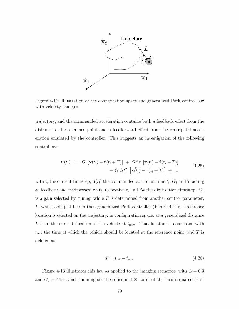
velocity in configuration-space (Figure 4-11), of magnitude:
||u|| = 2x2
Lsin η (4.24)
where η is the generalized angle and x is the generalized velocity in configuration-
space. This acceleration has a component in velocity-space, added parallel to the
velocity and a component in position-space, added perpendicular to the velocity.
When the current velocity of the vehicle corresponds to the velocity required to join
the current position to the target position along circular arc of radius L, with mag-
nitude equal to that at the target velocity, the law reduces to the Park law from [26],
as might be expected.
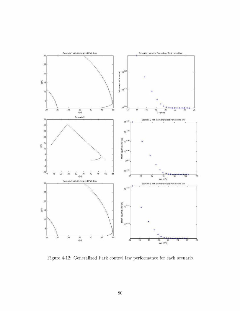
Figure 4-12 illustrates the performance of this law for each scenario. The perfor-
mance of the scenario 2 case is greatly improved by the ability to vary the velocity,
but suffers still from the discontinuities in the derivatives of the reference trajectory.
4.3.2 Anticipation
The Park control law is successful in reducing tracking errors and fuel use by select-
ing a reference point in the future of the trajectory and using that information to
anticipate future accelerations the vehicle will be subjected to. The parameter L acts
as a gain by selecting a reference point at a variable distance in the future of the
77
Figure 4-10: Park control law performance for each scenario
78
Figure 4-11: Illustration of the configuration space and generalized Park control lawwith velocity changes
trajectory, and the commanded acceleration contains both a feedback effect from the
distance to the reference point and a feedforward effect from the centripetal accel-
eration emulated by the controller. This suggests an investigation of the following
control law:
u(ti) = G [x(ti)− r(ti + T )] + G∆t [x(ti)− r(ti + T )]
+ G ∆t2[
¨x(ti)− r(ti + T )]
+ ...(4.25)
with ti the current timestep, u(ti) the commanded control at time ti, G1 and T acting
as feedback and feedforward gains respectively, and ∆t the digitization timestep. G1
is a gain selected by tuning, while T is determined from another control parameter,
L, which acts just like in then generalized Park controller (Figure 4-11): a reference
location is selected on the trajectory, in configuration space, at a generalized distance
L from the current location of the vehicle at tnow. That location is associated with
tref , the time at which the vehicle should be located at the reference point, and T is
defined as:
T = tref − tnow (4.26)
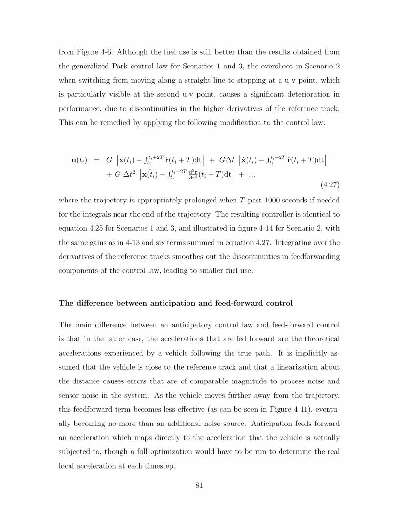
Figure 4-13 illustrates this law as applied to the imaging scenarios, with L = 0.3
and G1 = 44.13 and summing six the series in 4.25 to meet the mean-squared error
79
Figure 4-12: Generalized Park control law performance for each scenario
80
from Figure 4-6. Although the fuel use is still better than the results obtained from
the generalized Park control law for Scenarios 1 and 3, the overshoot in Scenario 2
when switching from moving along a straight line to stopping at a u-v point, which
is particularly visible at the second u-v point, causes a significant deterioration in
performance, due to discontinuities in the higher derivatives of the reference track.
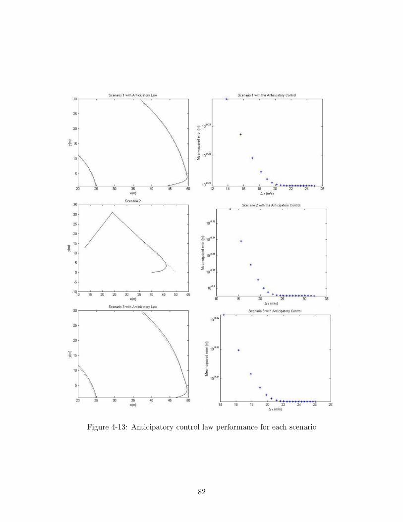
This can be remedied by applying the following modification to the control law:
u(ti) = G[x(ti)−
∫ ti+2Tti
r(ti + T )dt]
+ G∆t[x(ti)−
∫ ti+2Tti
r(ti + T )dt]
+ G ∆t2[
¨x(ti)−∫ ti+2Tti
d3rdt3
(ti + T )dt]
+ ...
(4.27)
where the trajectory is appropriately prolonged when T past 1000 seconds if needed
for the integrals near the end of the trajectory. The resulting controller is identical to
equation 4.25 for Scenarios 1 and 3, and illustrated in figure 4-14 for Scenario 2, with
the same gains as in 4-13 and six terms summed in equation 4.27. Integrating over the
derivatives of the reference tracks smoothes out the discontinuities in feedforwarding
components of the control law, leading to smaller fuel use.
The difference between anticipation and feed-forward control
The main difference between an anticipatory control law and feed-forward control
is that in the latter case, the accelerations that are fed forward are the theoretical
accelerations experienced by a vehicle following the true path. It is implicitly as-
sumed that the vehicle is close to the reference track and that a linearization about
the distance causes errors that are of comparable magnitude to process noise and
sensor noise in the system. As the vehicle moves further away from the trajectory,
this feedforward term becomes less effective (as can be seen in Figure 4-11), eventu-
ally becoming no more than an additional noise source. Anticipation feeds forward
an acceleration which maps directly to the acceleration that the vehicle is actually
subjected to, though a full optimization would have to be run to determine the real
local acceleration at each timestep.
81
Figure 4-13: Anticipatory control law performance for each scenario
82
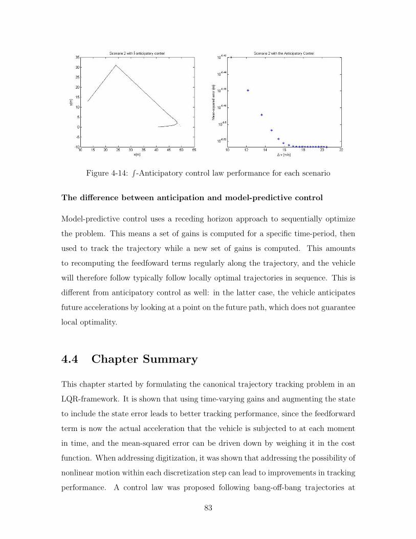
Figure 4-14:∫-Anticipatory control law performance for each scenario
The difference between anticipation and model-predictive control
Model-predictive control uses a receding horizon approach to sequentially optimize
the problem. This means a set of gains is computed for a specific time-period, then
used to track the trajectory while a new set of gains is computed. This amounts
to recomputing the feedfoward terms regularly along the trajectory, and the vehicle
will therefore follow typically follow locally optimal trajectories in sequence. This is
different from anticipatory control as well: in the latter case, the vehicle anticipates
future accelerations by looking at a point on the future path, which does not guarantee
local optimality.
4.4 Chapter Summary
This chapter started by formulating the canonical trajectory tracking problem in an
LQR-framework. It is shown that using time-varying gains and augmenting the state
to include the state error leads to better tracking performance, since the feedforward
term is now the actual acceleration that the vehicle is subjected to at each moment
in time, and the mean-squared error can be driven down by weighing it in the cost
function. When addressing digitization, it was shown that addressing the possibility of
nonlinear motion within each discretization step can lead to improvements in tracking
performance. A control law was proposed following bang-off-bang trajectories at
83
each timestep when feasible, and non-optimal weighted bang-off-bang trajectory when
the optimum is infeasible. To make use of another source of information not taken
advantage of by the standard LQR-framework, we introduced a nonlinear control
technique that makes use of information from the future of the track to determine
actuation commands. This technique was generalized to be usable in measurement-
based any design space, and used as an inspiration for anticipatory control methods.
These methods feed forward several derivatives of the reference trajectory at a point
at a variable time in the future of the trajectory to the controller, thereby anticipating
future accelerations stemming from curvature in the reference path. The technique
was further improved to handle discontinuities in the derivatives which caused a
deterioration in performance at corner-like conditions in the track.
Table 4.4 summarizes results from the scenarios over which all controllers were
evaluated. The gains in each controller were selected to meet the same mean-squared
error level. The best canonical technique from literature, Time-Varying LQ-Servo
control, does not perform as well as Bang-Off-Bang or Anticipatory control in the
context of these scenarios. The fact that the vehicle starts off the reference track,
a different location from that for which TV LQ-Servo gains were computed cause
the feedforward terms at the beginning of the trajectory to act as noise sources on
the trajectory. The table also includes the actual optimal fuel consumption for each
scenario.
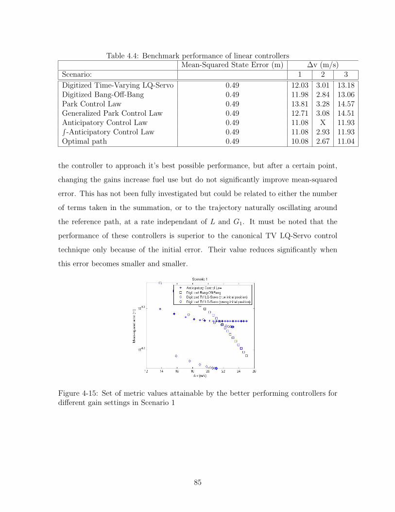
Figures 4-15, 4-16 and 4-17 illustrate the performance of the controllers in each
scenario. The figures show different possible performance levels of each controller
when the gains are varied. As a reference, the optimal performance, determined by
generating a TV LQ-Servo trajectory that starts off the reference track, is indicated
by the circles. The digitized Bang-Off-Bang control performance is closest to the
optimum when fuel use is heavily weighed. This is because the α and β parameters
can be tweaked so that the vehicle uses very little fuel until it reaches a point on the
reference trajectory, after which time the fuel use will be optimal. The anticipatory
approaches perform better than the Bang-Off-Bang control law for certain sets of
fuel use and mean-squared error values. Changing the L and G1 parameter causes
84
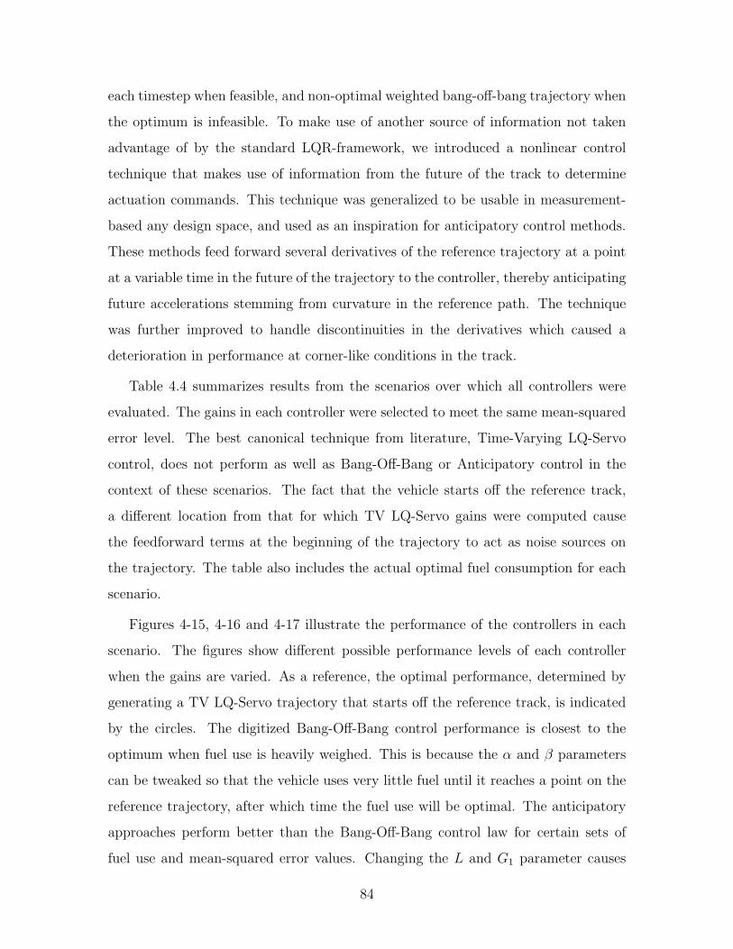
Table 4.4: Benchmark performance of linear controllersMean-Squared State Error (m) ∆v (m/s)
Scenario: 1 2 3
Digitized Time-Varying LQ-Servo 0.49 12.03 3.01 13.18Digitized Bang-Off-Bang 0.49 11.98 2.84 13.06Park Control Law 0.49 13.81 3.28 14.57Generalized Park Control Law 0.49 12.71 3.08 14.51Anticipatory Control Law 0.49 11.08 X 11.93∫-Anticipatory Control Law 0.49 11.08 2.93 11.93
Optimal path 0.49 10.08 2.67 11.04
the controller to approach it’s best possible performance, but after a certain point,
changing the gains increase fuel use but do not significantly improve mean-squared
error. This has not been fully investigated but could be related to either the number
of terms taken in the summation, or to the trajectory naturally oscillating around
the reference path, at a rate independant of L and G1. It must be noted that the
performance of these controllers is superior to the canonical TV LQ-Servo control
technique only because of the initial error. Their value reduces significantly when
this error becomes smaller and smaller.
Figure 4-15: Set of metric values attainable by the better performing controllers fordifferent gain settings in Scenario 1
85
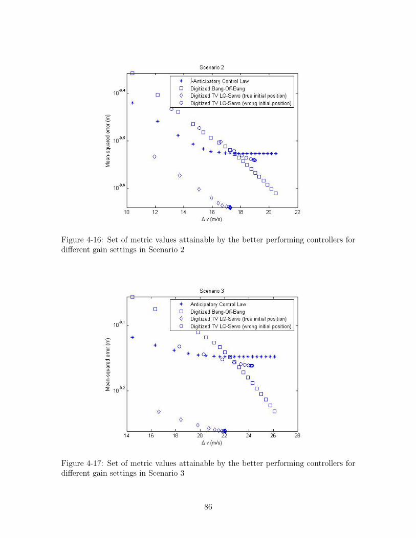
Figure 4-16: Set of metric values attainable by the better performing controllers fordifferent gain settings in Scenario 2
Figure 4-17: Set of metric values attainable by the better performing controllers fordifferent gain settings in Scenario 3
86
Chapter 5
Simulations and Experimental
Results
This chapter uses the trajectories defined in Chapter 3, and for which controllers were
designed in Chapter 4, and applies them to a hardware testbed in a relevant environ-
ment. Effects due to control interaction with estimation, and to computation-induced
delay were not taken in to account when designing the trajectories and control laws,
and can only be evaluated by applying the techniques to a real-world system. This
chapter presents the SPHERES formation flight testbed, and its associated simula-
tion for algorithm development, and presents results from tests on board the space
station and compares them to simulation results.
5.1 Experimental Testbed
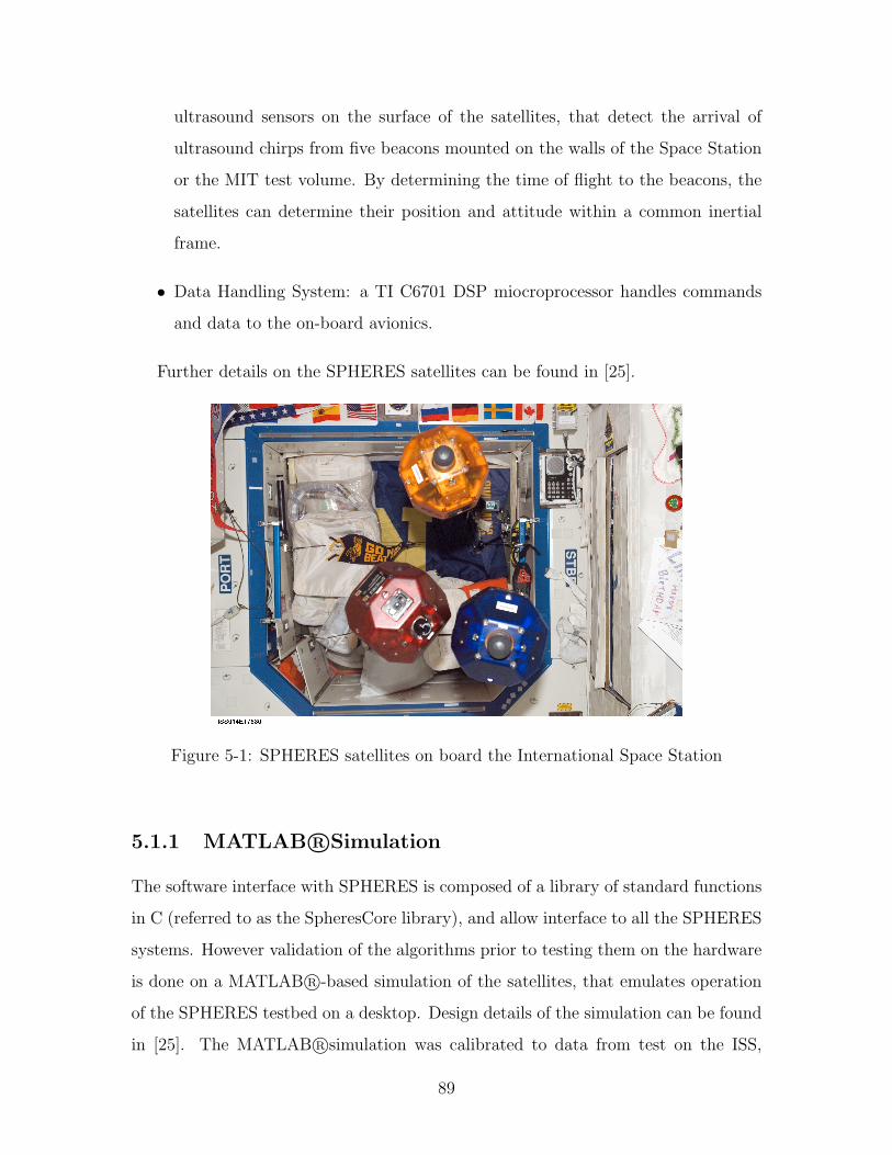
The Synchronized Position Hold Engage and Reorient Experimental Satellites (SPHERES)
facility (Figure 5-1) consists of 30cm-diameter nanosatellites acting as a satellite bus
in a six degree-of-freedom environment. Three satellites are currently on board the In-
ternational Space Station, and another three are kept in the MIT Space Systems Lab-
oratory. The testbed was designed to develop in-space formation flight, autonomous
docking, assembly and fault detection, isolation and recovery algorithms in a risk-
tolerant environment, with the possibility of iterative algorithm development and
87
reconfigurable testing, at a low cost (see [25]). The testing philosophy, when imple-
menting a new algorithm, is to develop a sequence of iterative steps to demonstrate
or validate all the properties of the algorithm, by increasing the complexity of the
algorithm in an incremental fashion: every test is slightly more complex than the
previous test, and is based on this previous test. This allows the researchers to test
algorithms to their limits, isolating their advantages and drawbacks and determining
the exact parameters within which an algorithm will work. For such an approach to
be successful, the hardware involved in algorithm development must be fault tolerant,
and present no risk to its operators. SPHERES satellites operating on board the ISS
or at the MIT ground facilities satisfy these two requirements: whenever off nominal
situations occur, the operator (or astronaut) can access the satellite and turn it off,
to determine what caused the problems to arise. In addition, the easy-access nature
of the hardware makes it possible to replenish consumables such as batteries and fuel
relatively simply. These two advantages of the SPHERES facility: fault-tolerance
and risk-tolerance, make it a unique testbed for experimentation in microgravity that
could not be replicated outside of the Space Station or on the ground.
The SPHERES satellites contain all the subsystems typical of a satellite bus:
• Communications System: Two RF transmitters communicate to a laptop oper-
ated by an astronaut in the ISS, or a computer accessed by an operator at the
MIT ground facilities, which transmit telemetry from the satellites and receives
commands from the computers.
• Propulsion System: The satellites are equipped with 12 solenoid thrusters, ac-
tuated electronically, that expel pressurized CO2 from a replaceable pressurized
gas cylinder.
• Power System: 16 AA replaceable batteries are housed within the satellite struc-
ture.
• Navigation System: the satellite can make use of inertial navigation systems:
three accelerometers and three gyroscopes provide attitude and positioning in-
formation. A GPS-like positioning system is also available, consisting of 24
88
ultrasound sensors on the surface of the satellites, that detect the arrival of
ultrasound chirps from five beacons mounted on the walls of the Space Station
or the MIT test volume. By determining the time of flight to the beacons, the
satellites can determine their position and attitude within a common inertial
frame.
• Data Handling System: a TI C6701 DSP miocroprocessor handles commands
and data to the on-board avionics.
Further details on the SPHERES satellites can be found in [25].
Figure 5-1: SPHERES satellites on board the International Space Station
with realistic sensor and actuator noise levels for the ultrasound sensors, thrusters
and gyroscopes. Computation and electronic delays are not taken into account, and
thruster reduction based on multiple thrusters opening at once were mapped on to
data obtained from ground testing. The current simulation does not model the com-
munication system and delays, rather making use of global variables in the function
files.
5.2 Array Retargetting
Formation retargeting maneuvers were tested during Test Session 7, on March 24,
2007, by astronauts Mike Lopez-Allegria and Sunita Williams; and during Test Ses-
sion 8, on April 27, 2007, by astronaut Sunita Williams. Tests included a 3-satellite
time-optimal trajectory (test session 7) and a rigid-array-equivalent trajectory (test
session 8), and were tracked using the SPHERES PID controller.
5.2.1 Fixed array
This test demonstrated a formation realignment maneuver during which the satellites
maintain the same relative distance to each other. For a rigidly-connected interfer-
ometer, each point on the surface of the instrument would follow a spherical helix arc,
when the interferometer is slewed. In the case of separated interferometers, following
such a trajectory will not be time or fuel optimal. However it allows to continue
observation of the astronomical target during the maneuver, since the relative dis-
tance between the spacecraft doesn’t change, so that the path length to the collector
wouldn’t change.
For this test, the satellites were deployed randomly in the volume. The satellites
first communicated their positions to each other, then moved to form an equilateral
triangle in the plane defined by their initial positions. The satellites would then
track a semi-circle at a rate of 0.33rpm, then slew the whole formation at a rate
of 0.66rpm while still continuing their relative 0.33rmp rotation. After rotated the
whole formation by π2, the formation continued along a circular trajectory for another
90
semi-circle. The satellites then stopped their motion.
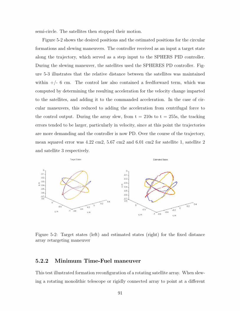
Figure 5-2 shows the desired positions and the estimated positions for the circular
formations and slewing maneuvers. The controller received as an input a target state
along the trajectory, which served as a step input to the SPHERS PID controller.
During the slewing maneuver, the satellites used the SPHERES PD controller. Fig-
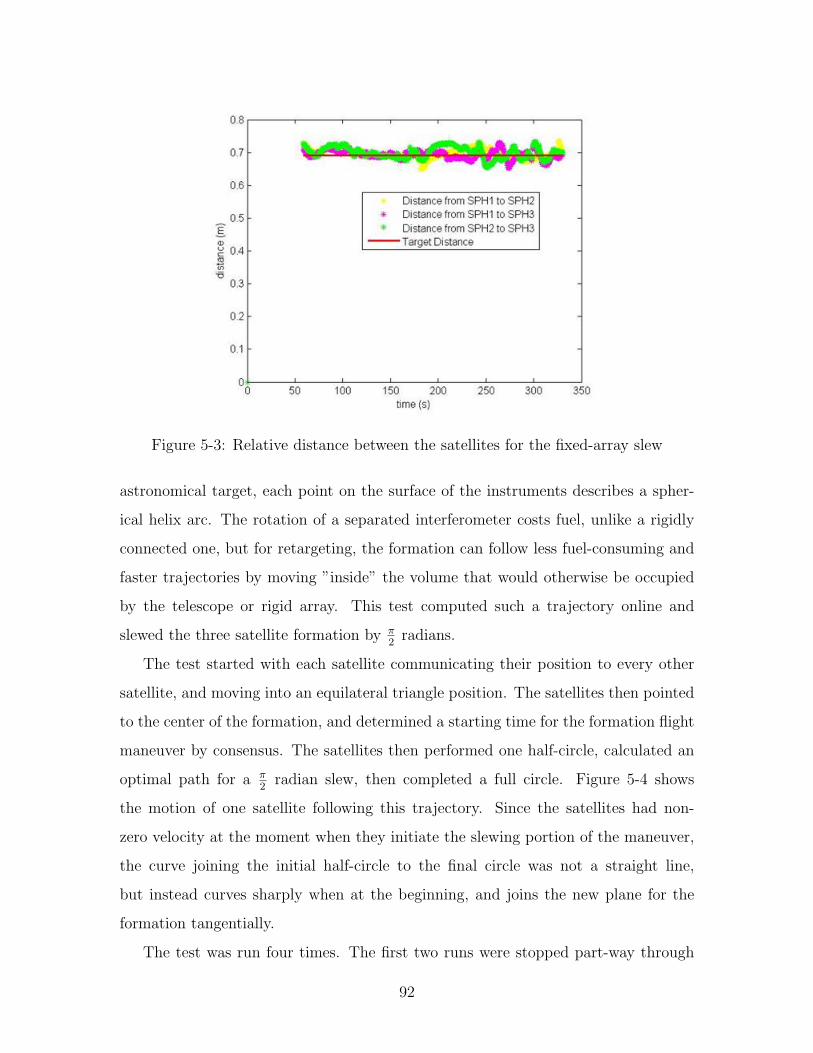
ure 5-3 illustrates that the relative distance between the satellites was maintained
within +/- 6 cm. The control law also contained a feedforward term, which was
computed by determining the resulting acceleration for the velocity change imparted
to the satellites, and adding it to the commanded acceleration. In the case of cir-
cular maneuvers, this reduced to adding the acceleration from centrifugal force to
the control output. During the array slew, from t = 210s to t = 255s, the tracking
errors tended to be larger, particularly in velocity, since at this point the trajectories
are more demanding and the controller is now PD. Over the course of the trajectory,
mean squared error was 4.22 cm2, 5.67 cm2 and 6.01 cm2 for satellite 1, satellite 2
and satellite 3 respectively.
Figure 5-2: Target states (left) and estimated states (right) for the fixed distancearray retargeting maneuver
5.2.2 Minimum Time-Fuel maneuver
This test illustrated formation reconfiguration of a rotating satellite array. When slew-
ing a rotating monolithic telescope or rigidly connected array to point at a different
91
Figure 5-3: Relative distance between the satellites for the fixed-array slew
astronomical target, each point on the surface of the instruments describes a spher-
ical helix arc. The rotation of a separated interferometer costs fuel, unlike a rigidly
connected one, but for retargeting, the formation can follow less fuel-consuming and
faster trajectories by moving ”inside” the volume that would otherwise be occupied
by the telescope or rigid array. This test computed such a trajectory online and
slewed the three satellite formation by π2
radians.
The test started with each satellite communicating their position to every other
satellite, and moving into an equilateral triangle position. The satellites then pointed
to the center of the formation, and determined a starting time for the formation flight
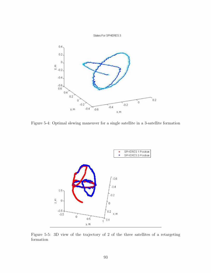
maneuver by consensus. The satellites then performed one half-circle, calculated an
optimal path for a π2
radian slew, then completed a full circle. Figure 5-4 shows
the motion of one satellite following this trajectory. Since the satellites had non-
zero velocity at the moment when they initiate the slewing portion of the maneuver,
the curve joining the initial half-circle to the final circle was not a straight line,
but instead curves sharply when at the beginning, and joins the new plane for the
formation tangentially.
The test was run four times. The first two runs were stopped part-way through
92
Figure 5-4: Optimal slewing maneuver for a single satellite in a 3-satellite formation
Figure 5-5: 3D view of the trajectory of 2 of the three satellites of a retargetingformation
93
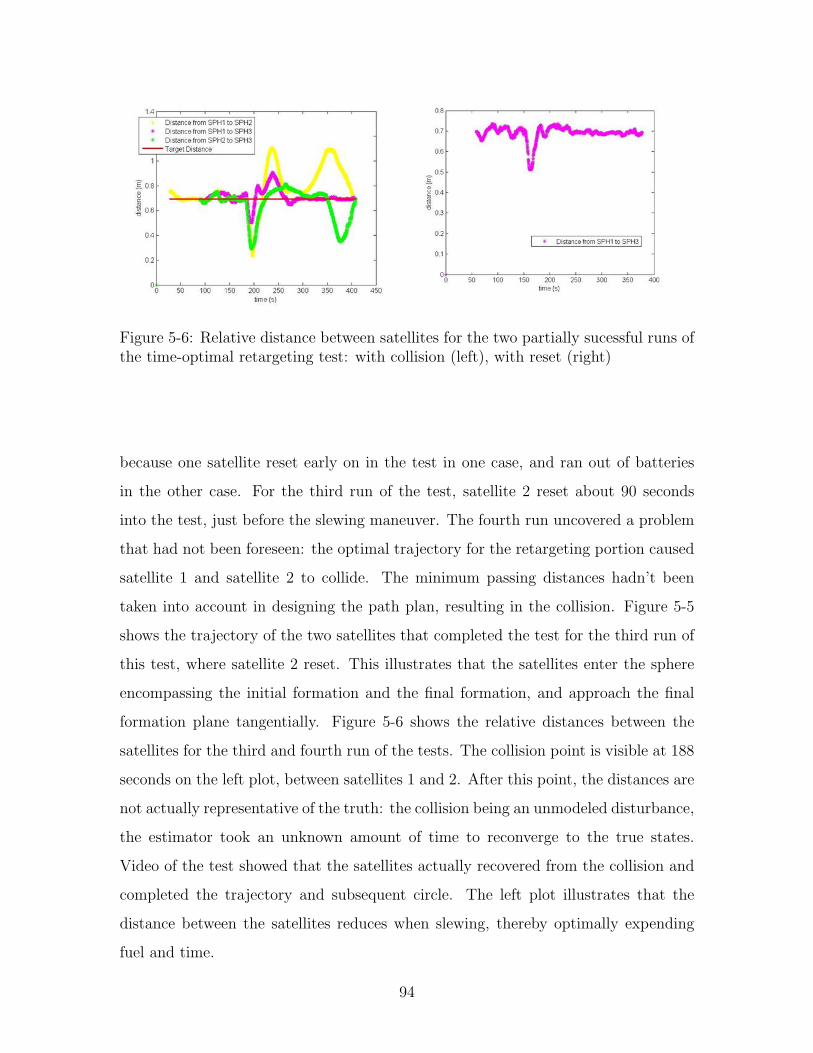
Figure 5-6: Relative distance between satellites for the two partially sucessful runs ofthe time-optimal retargeting test: with collision (left), with reset (right)
because one satellite reset early on in the test in one case, and ran out of batteries
in the other case. For the third run of the test, satellite 2 reset about 90 seconds
into the test, just before the slewing maneuver. The fourth run uncovered a problem
that had not been foreseen: the optimal trajectory for the retargeting portion caused
satellite 1 and satellite 2 to collide. The minimum passing distances hadn’t been
taken into account in designing the path plan, resulting in the collision. Figure 5-5
shows the trajectory of the two satellites that completed the test for the third run of
this test, where satellite 2 reset. This illustrates that the satellites enter the sphere
encompassing the initial formation and the final formation, and approach the final
formation plane tangentially. Figure 5-6 shows the relative distances between the
satellites for the third and fourth run of the tests. The collision point is visible at 188
seconds on the left plot, between satellites 1 and 2. After this point, the distances are
not actually representative of the truth: the collision being an unmodeled disturbance,
the estimator took an unknown amount of time to reconverge to the true states.
Video of the test showed that the satellites actually recovered from the collision and
completed the trajectory and subsequent circle. The left plot illustrates that the
distance between the satellites reduces when slewing, thereby optimally expending
fuel and time.
94
5.3 Fuel Balancing
Fuel balancing maneuvers were tested during Test Session 14, on October 26, October
27 and November 1 2008, by astronaut Greg Chamitoff. A simple fuel-balancing path
computed offline and tracked with PID control was attempted, as a preliminary test
for fuel-balancing algorithms.
5.3.1 ISS Results
This test was designed to be the first in a series aimed at demonstrating fuel-balancing
trajectories in space. A trajectory was designed offline to balance the amount of pro-
pellant in three satellites while they perform a spiral maneuver relative to each other,
by solving an optimization problem with an objective function penalizing tracking
error, fuel consumption as well as differences in propellant levels in the satellite tanks
as presented in Chapter 3. The test started with a 10-second maneuver during which
the satellites drift, to allow the estimator to converge. The satellites then pointed
to the center of the formation and went to initial positions, an equilateral triangle
in the Z = 0 frame in ISS coordinates, centered around the point (0.3, 0, 0). During
the next maneuver, the satellites tracked the pre-computed trajectory. Their motion
relative to each other was an Archimedean spiral, starting with a 50cm radius and
finishing with a 30cm radius after one rotation. The test concluded with a brief
stopping maneuver.
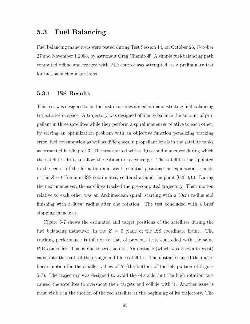
Figure 5-7 shows the estimated and target positions of the satellites during the
fuel balancing maneuver, in the Z = 0 plane of the ISS coordinate frame. The
tracking performance is inferior to that of previous tests controlled with the same
PID controller. This is due to two factors. An obstacle (which was known to exist)
came into the path of the orange and blue satellites. The obstacle caused the quasi-
linear motion for the smaller values of Y (the bottom of the left portion of Figure
5-7). The trajectory was designed to avoid the obstacle, but the high rotation rate
caused the satellites to overshoot their targets and collide with it. Another issue is
most visible in the motion of the red satellite at the beginning of its trajectory. The
95
target states constitute motion with a very small radius of curvature. Due to time
delays between computation of the desired control and actuation (which are tied to
the fact that the SPHERES estimator cannot run simultaneously with the actuators),
thrust was not direct in the desired direction, leading to tracking errors.
Figure 5-7: Estimated states (left) and target states (right) for the fuel-balancingmaneuver. Dotted triangles indicate the initial configuration of the formation (largertriangle) and the final configuration of the formation (smaller triangle).
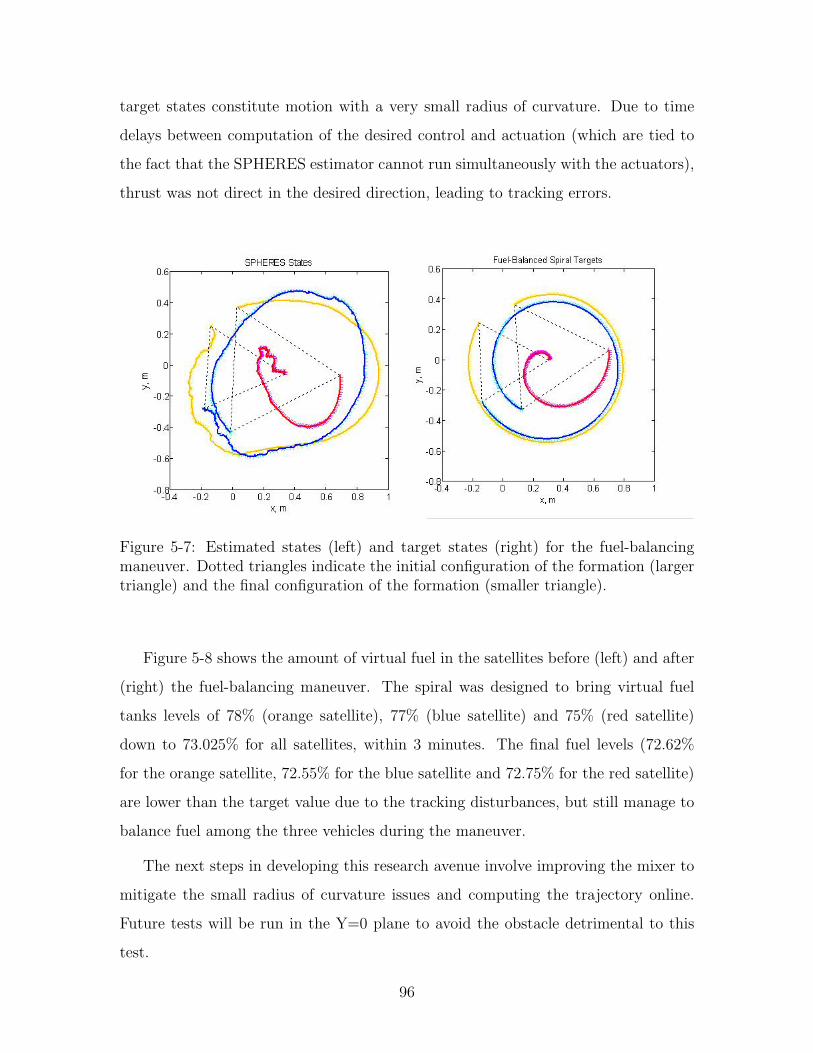
Figure 5-8 shows the amount of virtual fuel in the satellites before (left) and after
(right) the fuel-balancing maneuver. The spiral was designed to bring virtual fuel
tanks levels of 78% (orange satellite), 77% (blue satellite) and 75% (red satellite)
down to 73.025% for all satellites, within 3 minutes. The final fuel levels (72.62%
for the orange satellite, 72.55% for the blue satellite and 72.75% for the red satellite)
are lower than the target value due to the tracking disturbances, but still manage to
balance fuel among the three vehicles during the maneuver.
The next steps in developing this research avenue involve improving the mixer to
mitigate the small radius of curvature issues and computing the trajectory online.
Future tests will be run in the Y=0 plane to avoid the obstacle detrimental to this
test.
96
Figure 5-8: Simulated fuel level in the satellites before (left) and after (right) the fuelbalancing maneuver
5.4 Chapter Summary
This chapter presented results from implementation of the algorithms exposed in
Chapters 3 and 4 on a hardware based testbed. The testbed and its associated sim-
ulation tools were first presented in the opening sections of this chapter, followed
by results from tests on the International Space Station. Implementation of array
retargeting maneuvers, both time-optimal and of the fixed-array type, demonstrated
the techniques from Chapter 3. Fuel-balancing maneuvers during imaging of an in-
terferometer were also presented, with results compared to simulations.
97
98
Chapter 6
Conclusions
6.1 Thesis Summary
The overall objective of this thesis was to investigate optimal resource management
techniques for separated spacecraft interferometers to successfully synthesize images.
Assuming optimal imaging configurations that satisfy astronomical requirements have
been selected, the following two issues were addressed:
• Developing a framework to manage fuel use among different spacecraft during
retargeting of formations, to maximize the number of observations that can be
taken
• Determining computationally efficient control techniques to minimize fuel use
while meeting image synthesis metrics
The following is a chapter-by-chapter summary of the research performed to meet
these objectives.
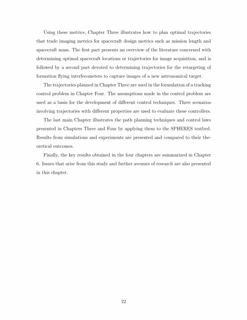
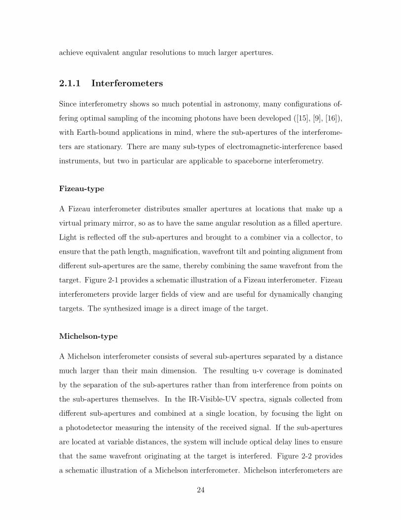
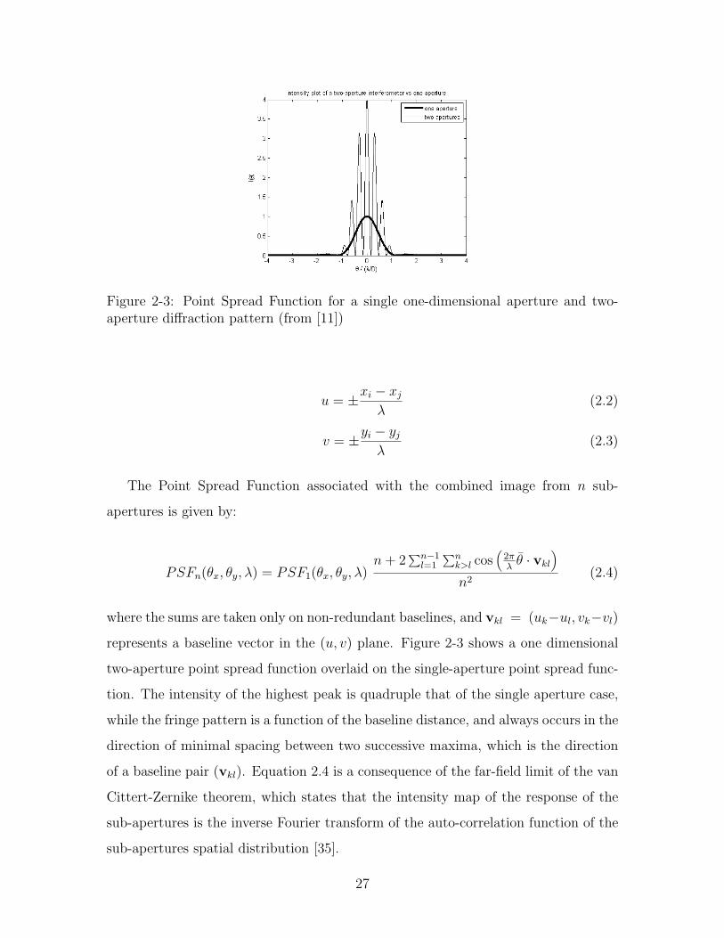
This thesis began with an overview of interferometry in Chapter 2. The point-
spread function as a measure of the quality of a synthesized image was presented,
and the associated metrics concerned with intensity and ambiguity were also ad-
dressed The complexity of these metrics motivated the presentation of a simplified
imaging-quality metric. Different interferometers were presented and the associated
technological developments needed were presented.
99
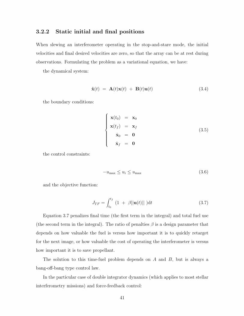
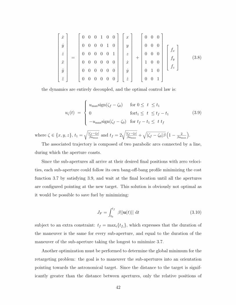
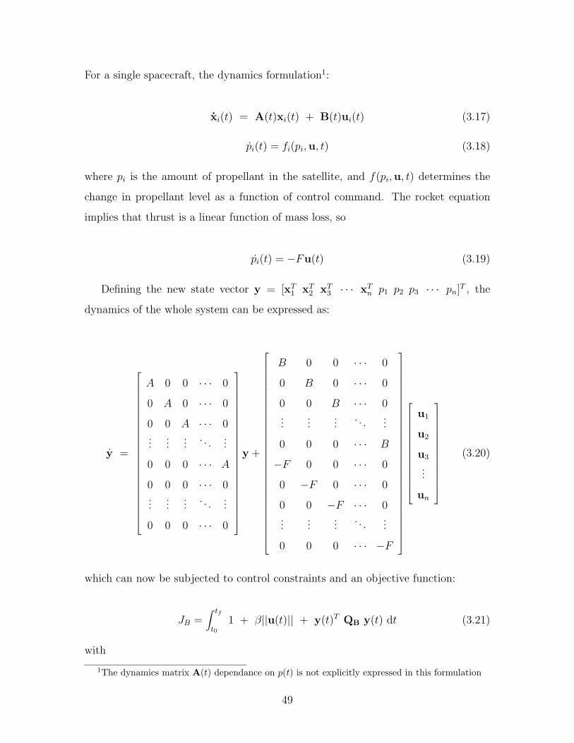
The imaging metrics were incorporated into an objective function in Chapter 3,
which became the basis for path planning techniques. After presenting stop-and-stare
and drift-through trajectories from the literature, these were furthered by determining
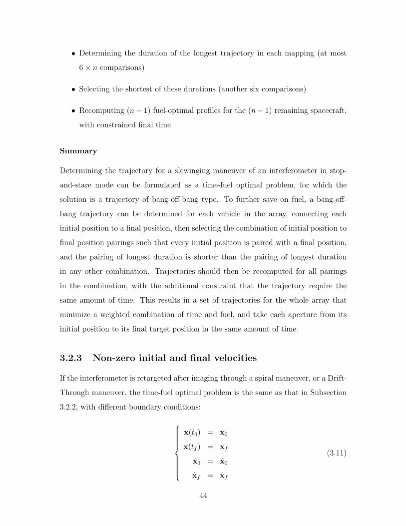
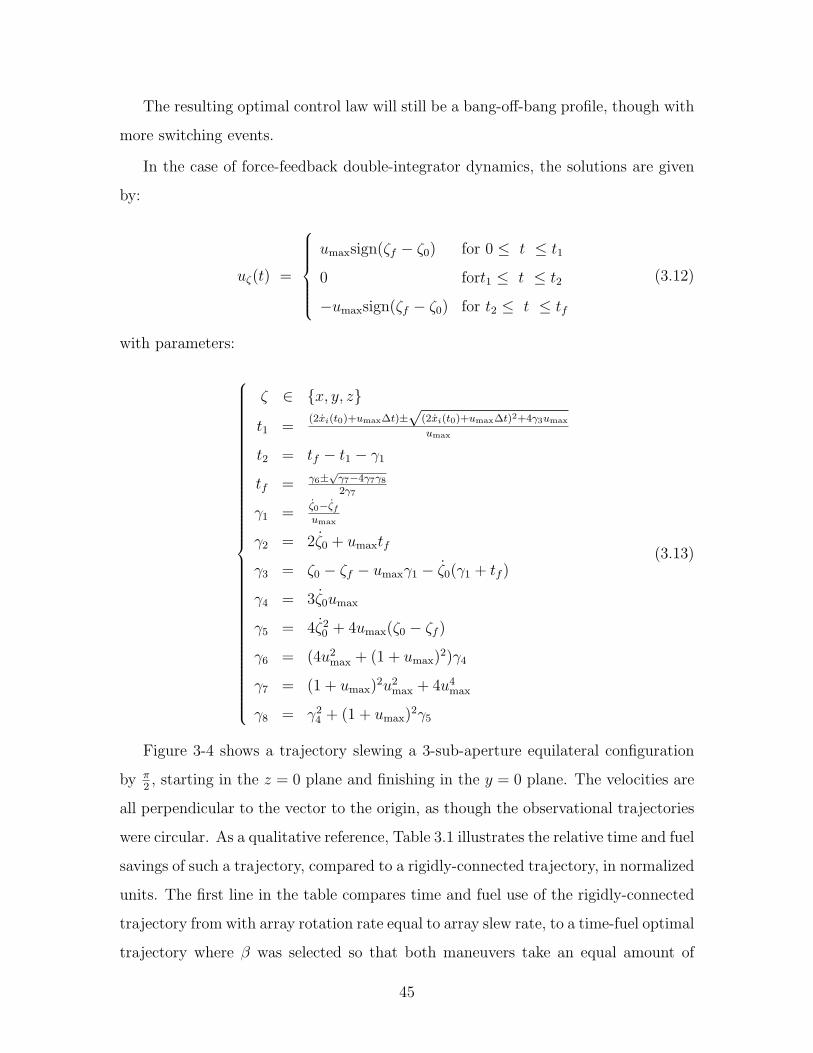
optimal trajectories for the retargetting of formation flying arrays to observe new
astronomical targets. The case of zero-velocity and non-zero-velocity initial and final
conditions were addressed, for stop-and-stare and on-the-fly imaging scenarios. After
observing that these retargeting trajectories lead to imbalances in fuel levels among
different satellites in the formation, a framework for the rebalancing of fuel among
satellites in a cluster was presented.
These trajectories were then used as reference inputs for control techniques in
Chapter 4. After summarizing the assumptions made by canonical linear control
techniques in the literature, the assumptions were challenged to attempt to derive
control laws with better tracking performance. A series of imaging scenarios were
presented and subjected to each control law. A new digitized bang-off-bang control
technique taking advantage of the nonlinearities induced by discretization, and a
technique furthering an approach that takes information from the future of the path
into account, were then defined and evaluated using representative scenarios.
Chapter 5 applied the developments from the previous chapters to a real system.
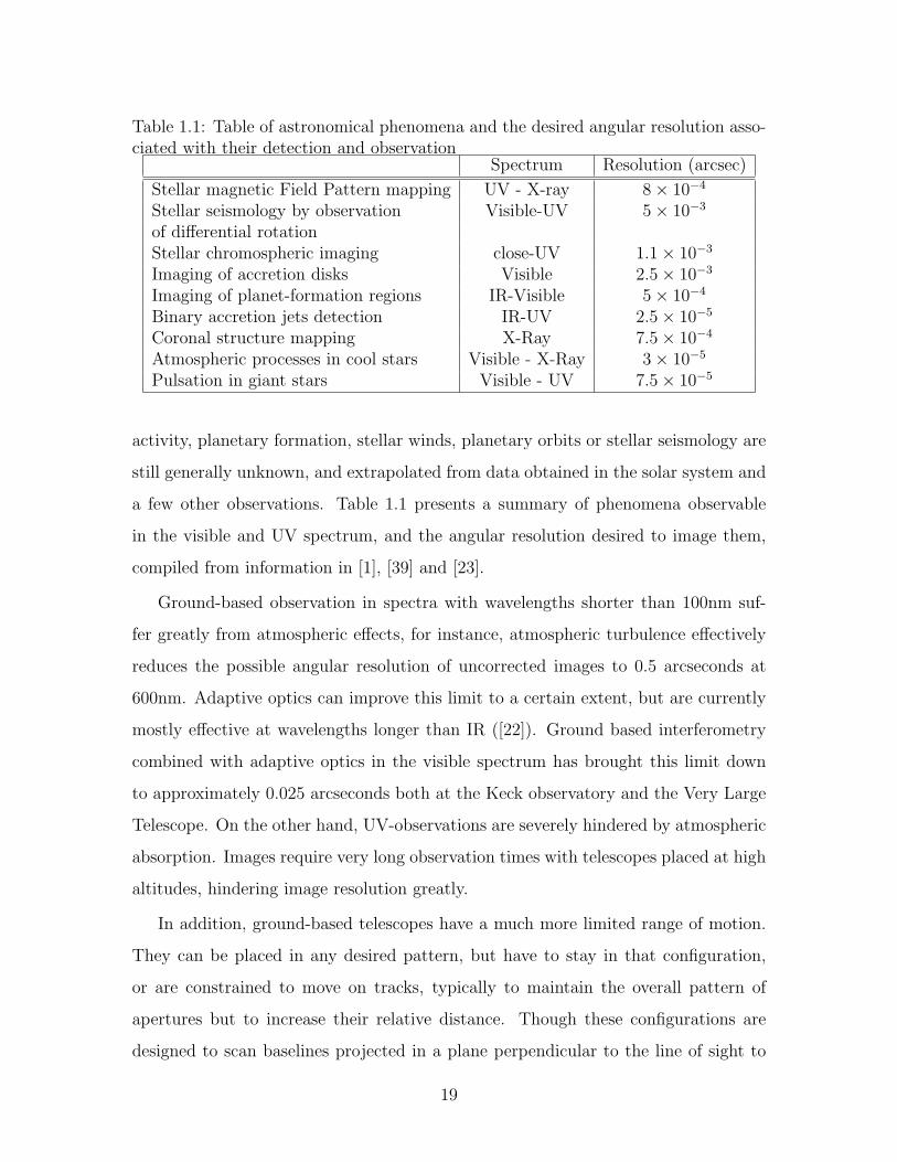
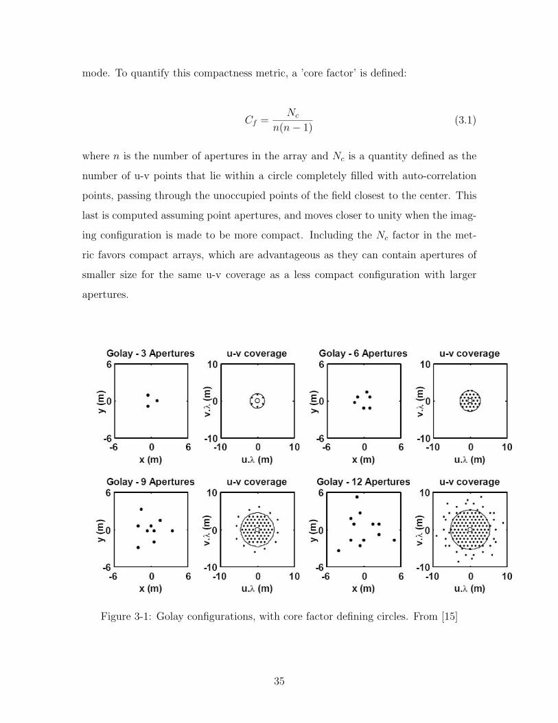
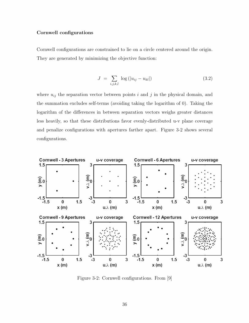
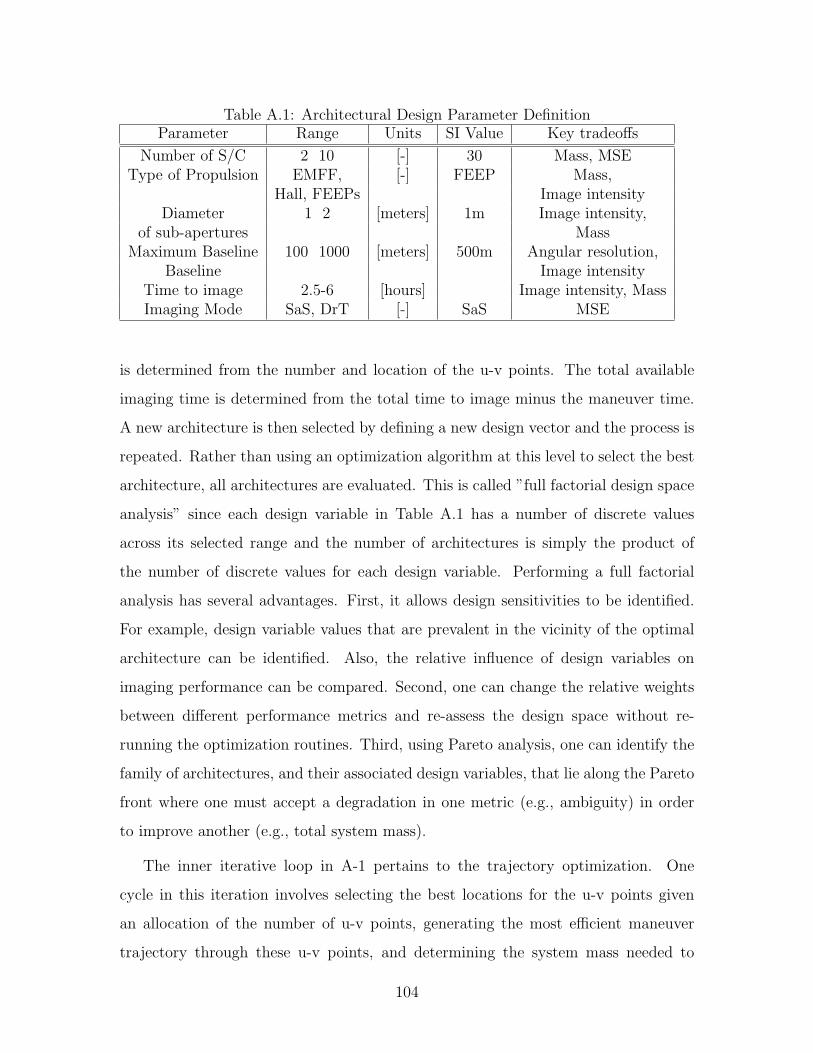
of sub-apertures MassMaximum Baseline 100 1000 [meters] 500m Angular resolution,
Baseline Image intensityTime to image 2.5-6 [hours] Image intensity, MassImaging Mode SaS, DrT [-] SaS MSE
is determined from the number and location of the u-v points. The total available
imaging time is determined from the total time to image minus the maneuver time.
A new architecture is then selected by defining a new design vector and the process is
repeated. Rather than using an optimization algorithm at this level to select the best
architecture, all architectures are evaluated. This is called ”full factorial design space
analysis” since each design variable in Table A.1 has a number of discrete values
across its selected range and the number of architectures is simply the product of
the number of discrete values for each design variable. Performing a full factorial
analysis has several advantages. First, it allows design sensitivities to be identified.
For example, design variable values that are prevalent in the vicinity of the optimal
architecture can be identified. Also, the relative influence of design variables on
imaging performance can be compared. Second, one can change the relative weights
between different performance metrics and re-assess the design space without re-
running the optimization routines. Third, using Pareto analysis, one can identify the
family of architectures, and their associated design variables, that lie along the Pareto
front where one must accept a degradation in one metric (e.g., ambiguity) in order
to improve another (e.g., total system mass).
The inner iterative loop in A-1 pertains to the trajectory optimization. One
cycle in this iteration involves selecting the best locations for the u-v points given
an allocation of the number of u-v points, generating the most efficient maneuver
trajectory through these u-v points, and determining the system mass needed to
104
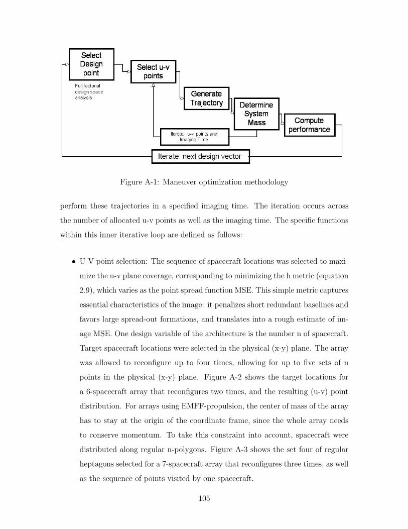
Figure A-1: Maneuver optimization methodology
perform these trajectories in a specified imaging time. The iteration occurs across
the number of allocated u-v points as well as the imaging time. The specific functions
within this inner iterative loop are defined as follows:
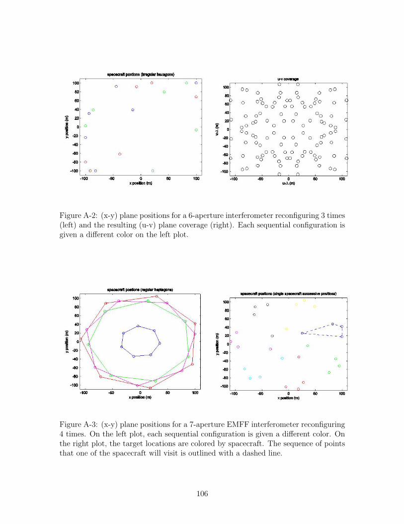
• U-V point selection: The sequence of spacecraft locations was selected to maxi-
mize the u-v plane coverage, corresponding to minimizing the h metric (equation
2.9), which varies as the point spread function MSE. This simple metric captures
essential characteristics of the image: it penalizes short redundant baselines and
favors large spread-out formations, and translates into a rough estimate of im-
age MSE. One design variable of the architecture is the number n of spacecraft.
Target spacecraft locations were selected in the physical (x-y) plane. The array
was allowed to reconfigure up to four times, allowing for up to five sets of n
points in the physical (x-y) plane. Figure A-2 shows the target locations for
a 6-spacecraft array that reconfigures two times, and the resulting (u-v) point
distribution. For arrays using EMFF-propulsion, the center of mass of the array
has to stay at the origin of the coordinate frame, since the whole array needs
to conserve momentum. To take this constraint into account, spacecraft were
distributed along regular n-polygons. Figure A-3 shows the set four of regular
heptagons selected for a 7-spacecraft array that reconfigures three times, as well
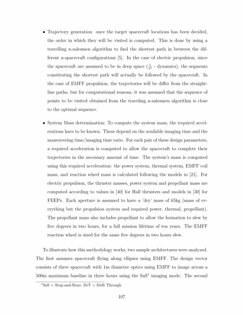
as the sequence of points visited by one spacecraft.
105
Figure A-2: (x-y) plane positions for a 6-aperture interferometer reconfiguring 3 times(left) and the resulting (u-v) plane coverage (right). Each sequential configuration isgiven a different color on the left plot.
Figure A-3: (x-y) plane positions for a 7-aperture EMFF interferometer reconfiguring4 times. On the left plot, each sequential configuration is given a different color. Onthe right plot, the target locations are colored by spacecraft. The sequence of pointsthat one of the spacecraft will visit is outlined with a dashed line.
106
• Trajectory generation: once the target spacecraft locations has been decided,
the order in which they will be visited is computed. This is done by using a
travelling n-salesmen algorithm to find the shortest path in between the dif-
ferent n-spacecraft configurations [5]. In the case of electric propulsion, since
the spacecraft are assumed to be in deep space ( 1s2 - dynamics), the segments
constituting the shortest path will actually be followed by the spacecraft. In
the case of EMFF propulsion, the trajectories will be differ from the straight-
line paths, but for computational reasons, it was assumed that the sequence of
points to be visited obtained from the traveling n-salesmen algorithm is close
to the optimal sequence.
• System Mass determination: To compute the system mass, the required accel-
erations have to be known. These depend on the available imaging time and the
maneuvering time/imaging time ratio. For each pair of these design parameters,
a required acceleration is computed to allow the spacecraft to complete their
trajectories in the necessary amount of time. The system’s mass is computed
using this required acceleration: the power system, thermal system, EMFF coil
mass, and reaction wheel mass is calculated following the models in [21]. For
electric propulsion, the thruster masses, power system and propellant mass are
computed according to values in [40] for Hall thrusters and models in [30] for
FEEPs. Each aperture is assumed to have a ’dry’ mass of 65kg (mass of ev-
erything but the propulsion system and required power, thermal, propellant).
The propellant mass also includes propellant to allow the formation to slew by
five degrees in two hours, for a full mission lifetime of ten years. The EMFF
reaction wheel is sized for the same five degrees in two hours slew.
To illustrate how this methodology works, two sample architectures were analyzed.
The first assumes spacecraft flying along ellipses using EMFF. The design vector
consists of three spacecraft with 1m diameter optics using EMFF to image across a
500m maximum baseline in three hours using the SaS1 imaging mode. The second
1SaS = Stop-and-Stare, DrT = Drift Through
107
sample architecture uses five spacecraft with 2m diameter mirrors to move across a
100m maximum baseline using FEEPs propulsion. Table A.2 lists the design vector
values for each of these two architectures along with the performance outputs. Notice
that these are two very different architectures. The first design, using EMFF has
better angular resolution (larger maximum baseline) and more u-v points but the
imaging time is poorer. The spacecraft mass for a ten-year mission using FEEPs in
the second design is substantially heavier. However, it spends more time imaging since
it is only maneuvering over a small baseline. As a result, it is difficult to compare
these two designs since they both have strengths and weaknesses and we need to
broadly analyze the larger trade-space.
Table A.2: Design vector inputs and performance metric outputs for two samplearchitectures
Design 1 Design 2
Design Vector ValuesNumber of S/C 3 5
Type of propulsion EMFF FEEPsDiameter of sub-apertures 1.0 m 2.0 m
Maximum baseline 500 m 100 mTime to image 3.0 hrs 6.0 hrsImaging mode SaS SaSPerformance
S/C mass 430 kg 780 kgPropulsion system mass 54 kg 22 kg
Angular resolution 417 m 97 mIntensity 0.07 % 0.51%
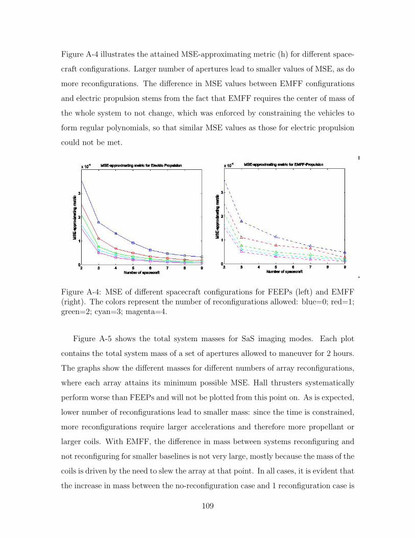
Figure A-4 illustrates the attained MSE-approximating metric (h) for different space-
craft configurations. Larger number of apertures lead to smaller values of MSE, as do
more reconfigurations. The difference in MSE values between EMFF configurations
and electric propulsion stems from the fact that EMFF requires the center of mass of
the whole system to not change, which was enforced by constraining the vehicles to
form regular polynomials, so that similar MSE values as those for electric propulsion
could not be met.
Figure A-4: MSE of different spacecraft configurations for FEEPs (left) and EMFF(right). The colors represent the number of reconfigurations allowed: blue=0; red=1;green=2; cyan=3; magenta=4.
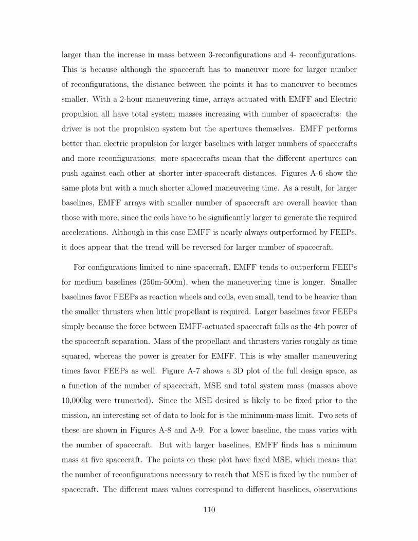
Figure A-5 shows the total system masses for SaS imaging modes. Each plot
contains the total system mass of a set of apertures allowed to maneuver for 2 hours.
The graphs show the different masses for different numbers of array reconfigurations,
where each array attains its minimum possible MSE. Hall thrusters systematically
perform worse than FEEPs and will not be plotted from this point on. As is expected,
lower number of reconfigurations lead to smaller mass: since the time is constrained,
more reconfigurations require larger accelerations and therefore more propellant or
larger coils. With EMFF, the difference in mass between systems reconfiguring and
not reconfiguring for smaller baselines is not very large, mostly because the mass of the
coils is driven by the need to slew the array at that point. In all cases, it is evident that
the increase in mass between the no-reconfiguration case and 1 reconfiguration case is
109
larger than the increase in mass between 3-reconfigurations and 4- reconfigurations.
This is because although the spacecraft has to maneuver more for larger number
of reconfigurations, the distance between the points it has to maneuver to becomes
smaller. With a 2-hour maneuvering time, arrays actuated with EMFF and Electric
propulsion all have total system masses increasing with number of spacecrafts: the
driver is not the propulsion system but the apertures themselves. EMFF performs
better than electric propulsion for larger baselines with larger numbers of spacecrafts
and more reconfigurations: more spacecrafts mean that the different apertures can
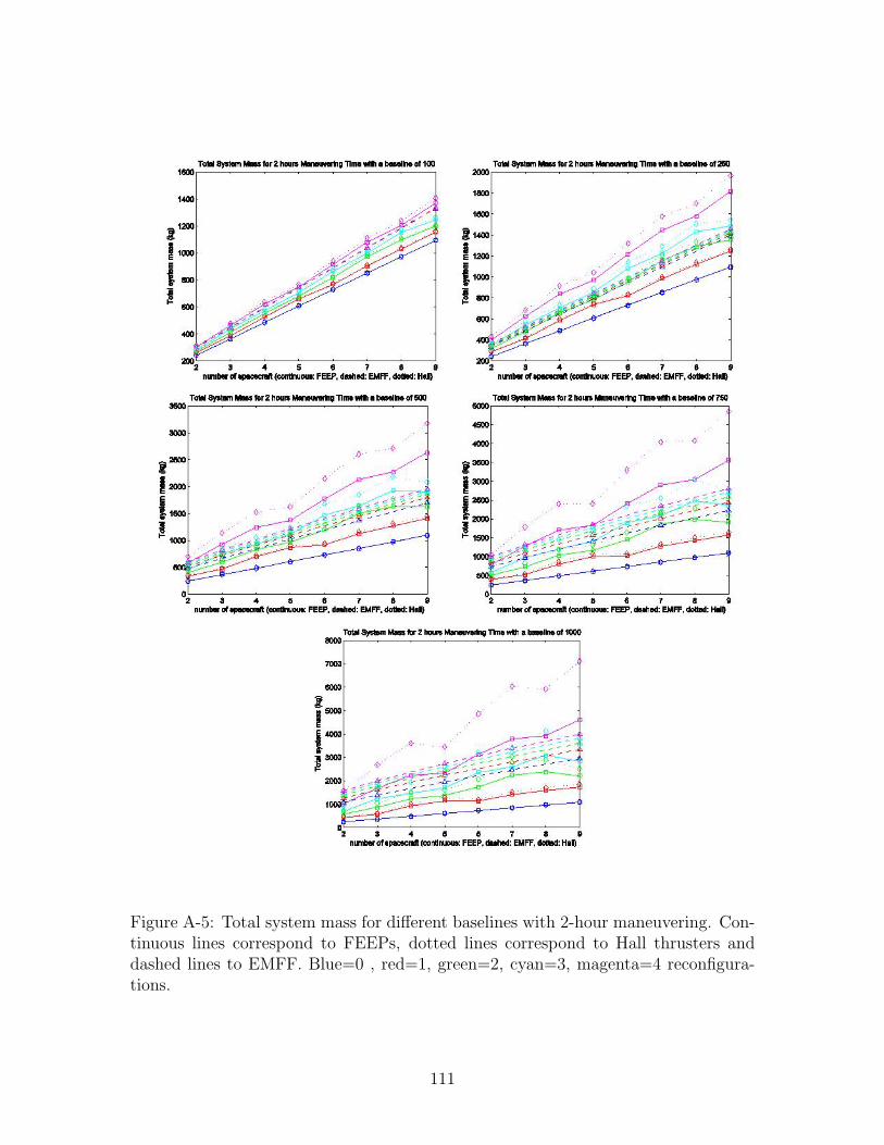
push against each other at shorter inter-spacecraft distances. Figures A-6 show the
same plots but with a much shorter allowed maneuvering time. As a result, for larger
baselines, EMFF arrays with smaller number of spacecraft are overall heavier than
those with more, since the coils have to be significantly larger to generate the required
accelerations. Although in this case EMFF is nearly always outperformed by FEEPs,
it does appear that the trend will be reversed for larger number of spacecraft.
For configurations limited to nine spacecraft, EMFF tends to outperform FEEPs
for medium baselines (250m-500m), when the maneuvering time is longer. Smaller
baselines favor FEEPs as reaction wheels and coils, even small, tend to be heavier than
the smaller thrusters when little propellant is required. Larger baselines favor FEEPs
simply because the force between EMFF-actuated spacecraft falls as the 4th power of
the spacecraft separation. Mass of the propellant and thrusters varies roughly as time
squared, whereas the power is greater for EMFF. This is why smaller maneuvering
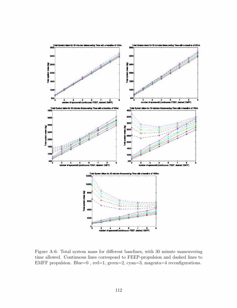
times favor FEEPs as well. Figure A-7 shows a 3D plot of the full design space, as
a function of the number of spacecraft, MSE and total system mass (masses above
10,000kg were truncated). Since the MSE desired is likely to be fixed prior to the
mission, an interesting set of data to look for is the minimum-mass limit. Two sets of
these are shown in Figures A-8 and A-9. For a lower baseline, the mass varies with
the number of spacecraft. But with larger baselines, EMFF finds has a minimum
mass at five spacecraft. The points on these plot have fixed MSE, which means that
the number of reconfigurations necessary to reach that MSE is fixed by the number of
spacecraft. The different mass values correspond to different baselines, observations
110
Figure A-5: Total system mass for different baselines with 2-hour maneuvering. Con-tinuous lines correspond to FEEPs, dotted lines correspond to Hall thrusters anddashed lines to EMFF. Blue=0 , red=1, green=2, cyan=3, magenta=4 reconfigura-tions.
111
Figure A-6: Total system mass for different baselines, with 30 minute maneuveringtime allowed. Continuous lines correspond to FEEP-propulsion and dashed lines toEMFF propulsion. Blue=0 , red=1, green=2, cyan=3, magenta=4 reconfigurations.
112
times, imaging time/maneuvering time ratios etc The minimum mass configurations
all have smallest baseline and longest maneuvering time, but the minimum-mass limit
does not significantly change shape with either baseline or maneuvering time.
Figure A-7: Full trade space. Red=EMFF, blue=FEEPs.
Previous results all show that the minimum mass configuration is always a 2-
spacecraft array, if the metric for which one optimizes is MSE. But smaller numbers
of spacecraft suffer from images that have less intensity: the number of apertures
looking at the sky is smaller. Figure A-10 shows the extent of the tradespace explored
for the Mass, MSE and Intensity metrics. An interesting trade to look for is the
minimum mass configuration for fixed intensity and MSE. This trade can lead to
determining the amount of MSE or intensity that the system can gain per additional
kilogram of mass. Results show, for instance, that for a fixed value of MSE and a
fixed total amount of time available for maneuvering and observing, as the intensity
increases from 200 aperture minutes (an intensity equal to 200 times that of a single
mirror of the size of one of the apertures) to 4500 aperture minutes, the minimum
mass configuration shifts from 2-spacecraft arrays to 6-spacecraft arrays. This occurs
because arrays with smaller numbers of spacecraft have to spend longer observing to
reach the same intensity as larger arrays. Since the observation window is constrained,
113
Figure A-8: Section of the design space for a fixed MSE-approximation (0.7× 10⁻⁴)and baseline (100m) . The dotted lines show the minimum mass limit.
Figure A-9: Section of the design space for a fixed MSE-approximation (0.7e-4) andbaseline (1000m). The dotted lines show the minimum mass limit.
114
smaller arrays have to maneuver more quickly to allow for longer observation times,
leading to heavier propulsion systems.
Figure A-10: Full trade space showing mass, MSE and image intensity (aperture-minutes)
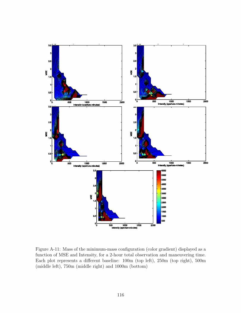
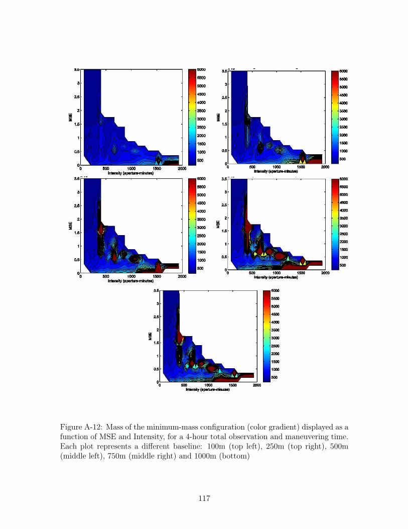
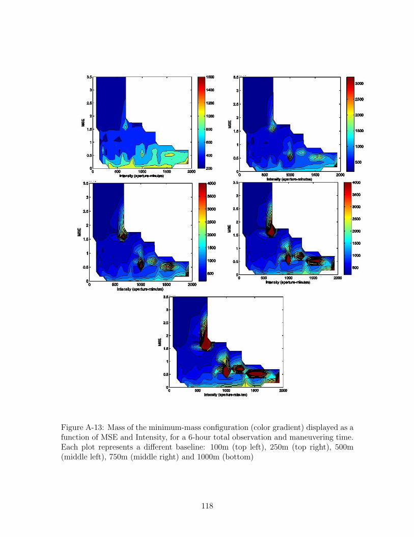
Figures A-11 to A-13 show the mass of the minimum mass configuration associ-
ated with a fixed MSE and Intensity, for all the baselines studied and total allowed
observation and maneuvering times. Such plots allow the designer to notice, for in-
stance, that with a 750m baseline and 6 hours imaging and observation time, the
performance of a design with 0.5 x 10⁻⁴ MSE and 700 aperture-minutes intensity can
be increased to 0.3 x 10⁻⁴ and 1000 aperture-minutes, with no extra penalty on mass.
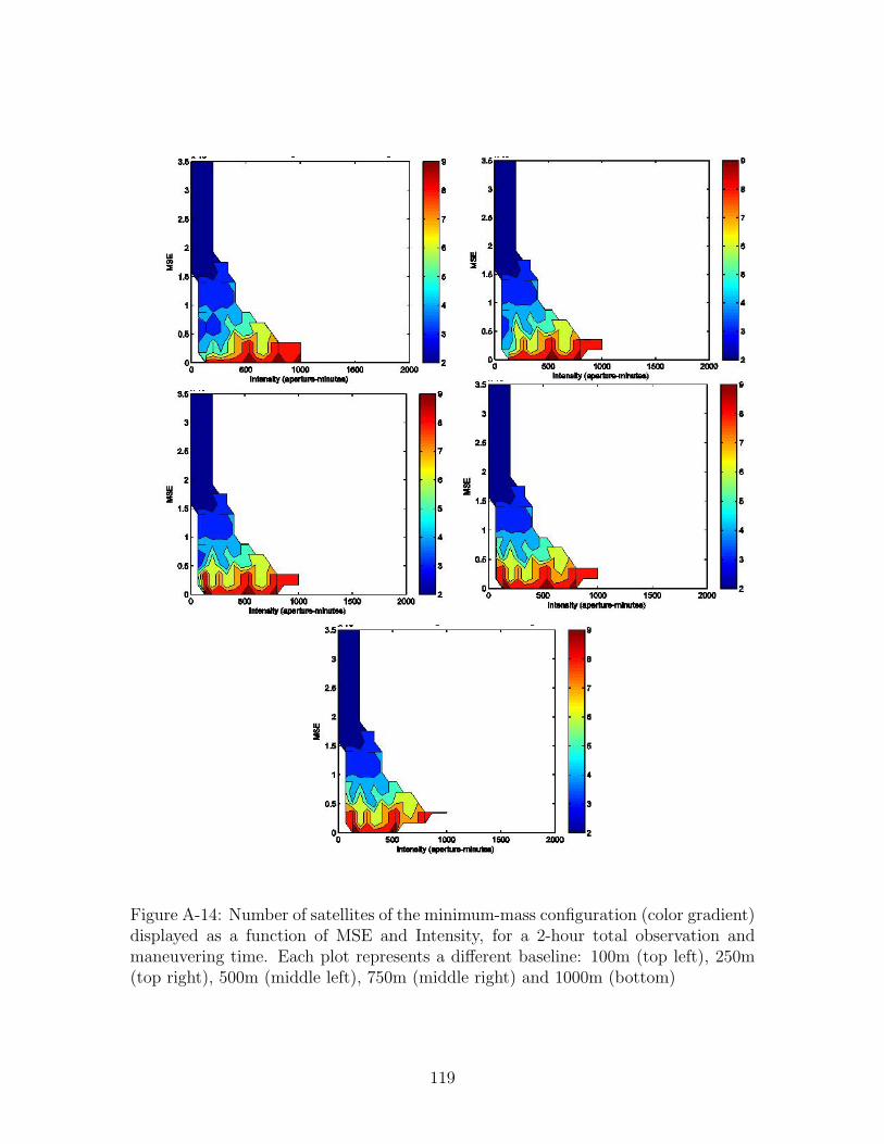
The number of spacecraft associated with the different minimum-mass configurations
for the baselines and allowed observation and maneuvering times are displayed in
Figures A-14 to A-16.
Switching from a Stop-and-Stare observation mode to a Drift-Through observation
mode is significantly reduces the total mass of the system. For this study, it was
assumed that a spacecraft requires 30 minutes integration time to interfere light for
one set of u-v points. The same trajectories can yield increases in image quality
as well as decreases in mass. Figure A-17 illustrate the reduction in total system
mass to obtain identical MSE values. The spacecraft were made to follow the same
115
Figure A-11: Mass of the minimum-mass configuration (color gradient) displayed as afunction of MSE and Intensity, for a 2-hour total observation and maneuvering time.Each plot represents a different baseline: 100m (top left), 250m (top right), 500m(middle left), 750m (middle right) and 1000m (bottom)
116
Figure A-12: Mass of the minimum-mass configuration (color gradient) displayed as afunction of MSE and Intensity, for a 4-hour total observation and maneuvering time.Each plot represents a different baseline: 100m (top left), 250m (top right), 500m(middle left), 750m (middle right) and 1000m (bottom)
117
Figure A-13: Mass of the minimum-mass configuration (color gradient) displayed as afunction of MSE and Intensity, for a 6-hour total observation and maneuvering time.Each plot represents a different baseline: 100m (top left), 250m (top right), 500m(middle left), 750m (middle right) and 1000m (bottom)
118
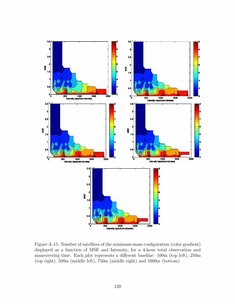
Figure A-14: Number of satellites of the minimum-mass configuration (color gradient)displayed as a function of MSE and Intensity, for a 2-hour total observation andmaneuvering time. Each plot represents a different baseline: 100m (top left), 250m(top right), 500m (middle left), 750m (middle right) and 1000m (bottom)
119
Figure A-15: Number of satellites of the minimum-mass configuration (color gradient)displayed as a function of MSE and Intensity, for a 4-hour total observation andmaneuvering time. Each plot represents a different baseline: 100m (top left), 250m(top right), 500m (middle left), 750m (middle right) and 1000m (bottom)
120
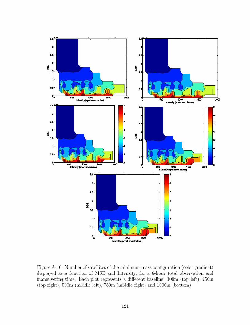
Figure A-16: Number of satellites of the minimum-mass configuration (color gradient)displayed as a function of MSE and Intensity, for a 6-hour total observation andmaneuvering time. Each plot represents a different baseline: 100m (top left), 250m(top right), 500m (middle left), 750m (middle right) and 1000m (bottom)
121
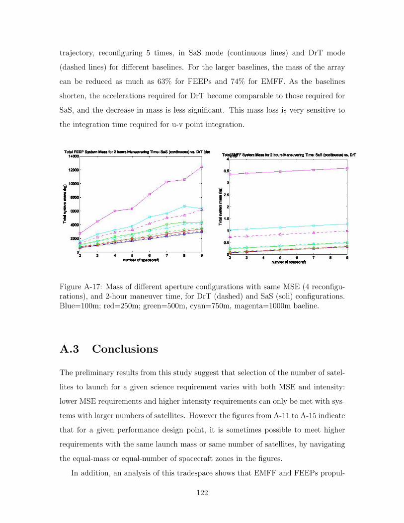
trajectory, reconfiguring 5 times, in SaS mode (continuous lines) and DrT mode
(dashed lines) for different baselines. For the larger baselines, the mass of the array
can be reduced as much as 63% for FEEPs and 74% for EMFF. As the baselines
shorten, the accelerations required for DrT become comparable to those required for
SaS, and the decrease in mass is less significant. This mass loss is very sensitive to
the integration time required for u-v point integration.
Figure A-17: Mass of different aperture configurations with same MSE (4 reconfigu-rations), and 2-hour maneuver time, for DrT (dashed) and SaS (soli) configurations.Blue=100m; red=250m; green=500m, cyan=750m, magenta=1000m baeline.
A.3 Conclusions
The preliminary results from this study suggest that selection of the number of satel-
lites to launch for a given science requirement varies with both MSE and intensity:
lower MSE requirements and higher intensity requirements can only be met with sys-
tems with larger numbers of satellites. However the figures from A-11 to A-15 indicate
that for a given performance design point, it is sometimes possible to meet higher
requirements with the same launch mass or same number of satellites, by navigating
the equal-mass or equal-number of spacecraft zones in the figures.
In addition, an analysis of this tradespace shows that EMFF and FEEPs propul-
122
sion systems can reach comparable total system masses for a large potion of the
tradespace, and EMFF generally weighs less for median baselines and larger satel-
lite numbers. For fixed MSE, minimum system masses are obtained for 2-spacecraft
arrays. The most significant metrics to trade are MSE and light intensity as higher
values of both lead to heavier systems, with larger numbers of spacecraft. Finally,
achieving Drift-Through imaging mode interferometry can lead to drastic decreases
in total system mass.
123
124
Bibliography
[1] SI - the stellar imager: Vision mission study report. NASA GSFC, September2005.
[2] Laser Interferometer Space Antenna (LISA) mission concept. NASA GSFC, May2008. LISA Project internal report number LISA-PRJ-RP-0001.
[3] R. W. Beard, T. W. McLain, and F. Y. Hadaegh. Fuel equalized retargetingfor separated spacecraft interferometry. In Proceedings of the American ControlConference, Philadelpha, PA, June 1998.
[4] R. W. Beard, T. W. McLain, and F. Y. Hadaegh. Fuel optimization for con-strained rotation of spacecraft formations. Journal of Guidance, Control andDynamics, 23(2), March-April 2000.
[5] D. P. Bertsekas. Nonlinear Programming. Athena Scientific, Belmont, MA, 2003.
[6] C. Beugnon, B. Calvel, S. Boulde, and F. Ankersen. Design and modeling ofthe formation-flying gnc system for the darwin interferometer. In Modeling andSystems Engineering for Astronomy, SPIE Proceedings, volume 5497, 2004.
[7] S. Chakravorty. Design and optimal control of Multi-spacecraft Interferometicimaging systems. PhD thesis, Univeristy of Michigan, Ann Arbor, MI, 2004.
[8] S. Chakravorty and J. L. Ramirez. Fuel optimal maneuvers for multispacecraftinterferometric imaging systems. Journal of Guidance, Control and Dynamics,30(1), January-February 2007.
[9] T. J. Cornwell. A novel principle for optmization of the instantaneous fourierplane coverage of correlation arrays. In IEEE Transactions on Antennas andPropagation, volume 36, August 1988.
[10] J. Deyst, J. P. How, and S. Park. Lyapunov stability of a nonlinear guidancelaw for uavs. In AIAA Atmospheric Flight Mechanics Conference and Exhibit,San Francisco, CA, August 2005.
[11] M. Diaz. Optimal interferometric maneuvers for distributed telescopes. Master’sthesis, SUPAERO, September 2008.
125
[12] R. E. Farley and D. A. Quinn. Tethered formation configurations: Meeting thescientific objectives of large aperture and interferometric science. In Proceedingsof the Second Workshop on New Concepts for Far-Infrared and SubmillimeterSpace Astronomy, College Park, MD, March 2002.
[13] G. F. Franklin and J. D. Powell. Digital Control of Dynamical Systems. AddisonWesley, Reading, MA, 1981.
[14] K. C. Gendreau, W. C. Cash, A. F. Shipley, and N. White. The maxim pathfinderx-ray interferometry mission. In SPIE Conference and Exhibit, Waikoloa, HI,September 2002.
[15] M. Golay. Point arrays having compact non-redundant autocorrelations. Journalof the Optical Society of America, 61, 1971.
[16] S. W. Golomb and H. Taylor. Two-dimensional synchronization patterns forminimum ambiguity. In IEEE Transactions on Information Theory, volume IT-28, July 1982.
[17] E. P. Goodwin and J. C. Wyant. Field Guide to Interferometric Optical Testing.SPIE Press, Bellingham, WA, 2006.
[18] D. E. Kirk. Optimal Control Theory. Dover Publications, New York, NY, 1970.
[19] E. M. C. Kong. Optimal trajectories and orbit design for separated spacecraftinterferometry. Master’s thesis, Massachusetts Institute of Technology, November1998.
[20] E. M. C. Kong. Spacecraft Formation Flight Exploiting Potential Fields. PhDthesis, Massachusetts Institute of Technology, February 2002.
[21] D. Kwon. Electromagnetic formation flight of satellite arrays. Master’s thesis,Massachusetts Institute of Technology, February 2005.
[22] Wizinowich P. L. Optical engineering at keck observatory : design and per-formance of the telescopes, adaptive optics and interferometer. In Proceedingsof SPIE Optical design and fabrication conference, volume 6034, Changchun,China, 2005.
[23] D. Leisawitz. Nasa’s far-ir/submillimeter roadmap missions: Safir and specs.Advances in Space Research, 34, 2004.
[24] D. W. Miller, O. L. de Weck, and S.-J. Chung. Introduction to optics, February2001. MIT SSL Documentation.
[25] S. Nolet. Development of a Guidance, Navigation adn Control Architecture andValidation Process Enabling Autonomous Docking to a Tumbling Satelite. PhDthesis, Massachusetts Institute of Technology, May 2007.
126
[26] S. Park, J. Deyst, and J. P. How. A new nonlinear guidance logic for trajectorytracking. In AIAA Guidance Navigation and Control Conference and Exhibit,August 2004.
[27] S. Park, J. Deyst, and J. P. How. Performance and Lyapunov stability of anonlinear path-following guidance method. Journal of Guidance, Control andDynamics, 30(6), November-December 2007.
[28] A. Rahmani, M. Mesbahi, and F. Hadaegh. Optimal balanced-energy formationflying maneuvers. Journal of Guidance, Control and Dynamics, 29(6), November-December 2006.
[29] C. L. Ranieri and C. A. Ocampo. Indirect optimization of spiral trajectories.Journal of Guidance, Control and Dynamics, 29(6), November-December 2006.
[30] J. G. Reichbach. Micropropulsion system selection for precision formation flyingsatellites. Master’s thesis, Massachusetts Institute of Technology, January 2001.
[31] R. J. Sedwick and D. W. Miller. System level design trades for the submillimiterprobe of the evolution of cosmic structures (specs). SSL Internal Report.
[32] T. Shimomura, Y. Yamazaki, and T. Fujii. Multi-stage control design of strictlypositive real h2 controllers. Transactions of the Institute of Systems, Control andInformation Engineers, 19(9), 2006.
[33] R. V. Stachnik, K. Ashlin, and S. Hamilton. Space station-samsi: a spacecraftarray for michelson spatial interferometry. Bulletin of the American AstronomicalSociety, 16(3), 1984.
[34] D. H. Staelin, J. W. Barrett, L. D. Clark, and B. E. Hines. Phase-coherentastrometric interferometry.
[35] A. R. Thompson, J. M. Moran, and G. W. Swenson Jr. Interferometry andsynthesis in radio astronomy. Wiley, New York, NY, 2001.
[36] S. C. Unwin and M Shao.
[37] S. Vatoux. Etude theorique et experimentale d’un interferometre stellaire optiquea usage spatial. PhD thesis, Universite Paris Sud, 1991.
[38] P. K. C. Wang and F. Y. Hadaegh. Minimum-fuel formation reconfiguration ofmultiple free-flying spacecraft. Journal of the Astronautical Sciences, 1999.
[39] M. Wehner, S. Moses, K. Kroening, and E. Johnson. Terrestrial planet finderspace vehicle architecture trades. In SPIE Conference on Astronomical Interfer-ometry, Kona, HI, March 1998.
[40] J. R. Wertz and W. J. Larson. Space Mission Analysis and Design. MicrocosmPress, Torrance, CA, 1999.