technische universiteit eindhoven I Trajectory planning and feedforward design for electromechanical motion systems Report nr. DCT 2003-08 Paul Lambrechts Email: P.F.Lambrechts @tue.d 17th February 2003 Abstract This report considers trajectory planning with given design constraints and design of an ap- propriate feedforward controller for single axis motion control. A motivation is given for using fourth order feedfonvard with fourth order trajectories. An algorithm is given for cal- culating hqjher order trajectories with bounds on all considered derivatives for point to point moves. It is shown that these trajectories are time-optimal in the most relevant cases. All required eqmtions for third and fourth order trajectory planning are explicitly derived. Im- plementation, discretization and quantization effects are considered. Simulation results show the effectiveness of fourth order feedfonvard in comparison with lower order feedforward.
Transcript
technische universiteit eindhoven
I
Trajectory planning and feedforward design for
electromechanical motion systems
Report nr. DCT 2003-08
Paul Lambrechts Email: P.F.Lambrechts @tue.d
17th February 2003
Abstract
This report considers trajectory planning with given design constraints and design of an ap- propriate feedforward controller for single axis motion control. A motivation is given for using fourth order feedfonvard with fourth order trajectories. An algorithm is given for cal- culating hqjher order trajectories with bounds on all considered derivatives for point to point moves. It is shown that these trajectories are time-optimal in the most relevant cases. All required eqmtions for third and fourth order trajectory planning are explicitly derived. Im- plementation, discretization and quantization effects are considered. Simulation results show the effectiveness of fourth order feedfonvard in comparison with lower order feedforward.
Contents
rn Introduction
Mass feedforward
Higher order feedforward
Higher order trajectory planning
Third order trajectory planning
Fourth order trajectory planning
Implementation aspects 7.1 Switching times 7.2 Synchronization of profiles 7.3 lmplementation of first order filter 7.4 Calculation of reference trajectory
Simulation results
Conclusions
1 Introduction
Feedforward control is a well known technique for high performance motion control problems as found in industry. It is, for instance, widely applied in robots, pick-and-place units and po- sitioning systems. These systems are often embedded in a factory automation scheme, which provides desired motion tasks to the considered system. Such a motion task can be to perform a motion from a position A to a position B, starbing at a time t. Usually this task is transferred to computer hardware dedicated to the control of the system, leaving the details of planning and execution of the motion to this dedicated motion control computer. The tasks of this dedicated motion controller will then consist of:
0 trajectory planning: the determination of an allowable trajectory for all degrees of freedom, separately or as a multidimensional trajectory, and the calculation of an allowable trajectory for each actuation device;
feedforward control: the representation of the desired trajectory in appropriate form and the calculation of a feedforward control signal for each actuation device, with the intention to obtain the desired trajectory;
0 system compensation: to reduce or remove unwanted behavior like known or measured disturbances and non-linearities;
feedback controk the processing of available measurements and calculation of a feedback control signal for each actuation device to compensate for unknown disturbances and un- modelled behavior,
internal checks, diagnostics, safety issues, communication, etc.
To simplify the tasks of the motion controller, the trajectory planning and feedforward control are usually done for each actuating device separately, relying on system compensation and feed- back control to deal with interactions and non-linearities. In that case, each actuating device is considered to be acting on a simple object, usually a single mass, moving along a single degree of freedom. The feedforward control problem is then to generate the force required to perform the acceleration of the mass in accordance with the desired trajectory. Conversely, the desired trajectory should be such that the required force is allowable (in the sense of mechanical load on the system) and can be generated by the actuating device. For obvious reasons this approach is of- ten referred to as 'mass feedforward' or 'rigid-body feedforward'. It allows a simple and practical implementation of both trajectory planning and feedforward control, as the required calculations are straightforward. The disadvantage of this approach is its dependence on system compensa- tion and feedback control to deal with unmodelled behavior as mentioned before. The resulting problem formulation can be split in two.
I. During execution of the trajectory the position errors are large, such that feedback con- trol actions are considerable. Actual velocity and acceleration (hence: actuator force) may therefore be much larger than planned. This may lead to undesired and even dangerous deviations from the planned trajectory and damage to actuator and system.
2. When arriving at the desired endpoint, the positioning error is large and the dynarnical state of the controlled system is not settled. Although the trajectory has finished, it is often necessary to wait for a considerable time before the position error is settled within
some given accuracy bounds before subsequent actions or motions are allowed. A practical consequence is the need for of a complex test to determine whether settling has sufficiently occurred. Furthermore, it is a source of time uncertainty that may be undesirable on the factory automation level.
To improve on this, many academic and practical approaches are possible. These can roughly be categorized in three.
I. Trajectory smoothing or shaping: This can be done by simply reducing the acceleration and velocity bounds used for trajectory planning, but also by smoothing or shaping the trajectory and/or application of force (higher order trajectories, S-curves, input shaping, filtering). The result of this can be very good, especially if the dynamical behavior of the motion system is explicitly taken into account. However, it may also lead to a considerable increase in execution time of the trajectory, often without a clear mechanism for finding a time optimal solution. Various examples of this approach can be found in [3,6,7,8,12,5].
2. Feedforward control based on plant inversion: This attempts to take the effect of unmod- elled behavior into account by either using a more detailed model of the motion system or by learning its behavior based on measurements. An important practical disadvantage is that they do not provide an approach for designing an appropriate trajectory. Various examples of this approach can be found in [2, 4, g, IO,II, 14,15,16].
3. Feedback control optimization (possibly aided by system compensation improvement): By improving the feedback controller, the positioning errors can be kept smaller during and at the end of the trajectory. Furthermore, settling will occur in a shorter time. Also in this case the design of an appropriate trajectory is not considered. Obviously, any feedback control design method can be used for this. Some references given above also include a discussion on the effect of feedback control on trajectory following; e.g. see [IO, 11,161.
This report will provide a method for higher order trajectory planning that can be used with all of the approaches given above. It is attempted to give a better understanding of the effect of smoothing, especially when considering a more optimal balancing between time optimality, physical bounds (actuator device and motion system limits) and accuracy. 'Fourth order feedfor- ward' wdl be presented as a clear and well implementable extension of 'mass feedforward', with also a clear strategy for obtaining the aforementioned optimal balance. The implementation of a fourth order trajectory planner will be set up as a natural extension of second and third order planners to show the potential for practical application. Furthermore, the calculation of the op- timal feedforward control signal will be shown. Next the effect of discrete time implementation will be considered: this includes the planning of a fourth order trajectory in discrete time and the optimal compensation of time delays in the feedforward control signal. Finally, some simulation results are given to further motivate the use of fourth order feedforward.
The next chapter will review mass feedforward, mostly with the purpose of introducing some notation. Next, chapter 3 will consider the extension of mass feedforward to fourth order feedfor- ward, based on an extended model of the motion system. A general algorithm for higher order trajectory planning will be considered in chapter 4, after which the relevant equations are derived for third order trajectory planning in chapter 5 and for fourth order trajectory planning in chap- ter 6. Next, implementation aspects are considered in chapter 7, followed by some simulation results in chapter 8, and conclusions in chapter g.
2 Mass feedforward
The specifics of planning a trajectory and calculating a feedforward signal based on mass feed- forward are fairly simple and can be found in many commercially available electromechanical motion control systems. In this chapter a short review is given as an introduction to a standard- ized approach to third and fourth order feedforward calculations.
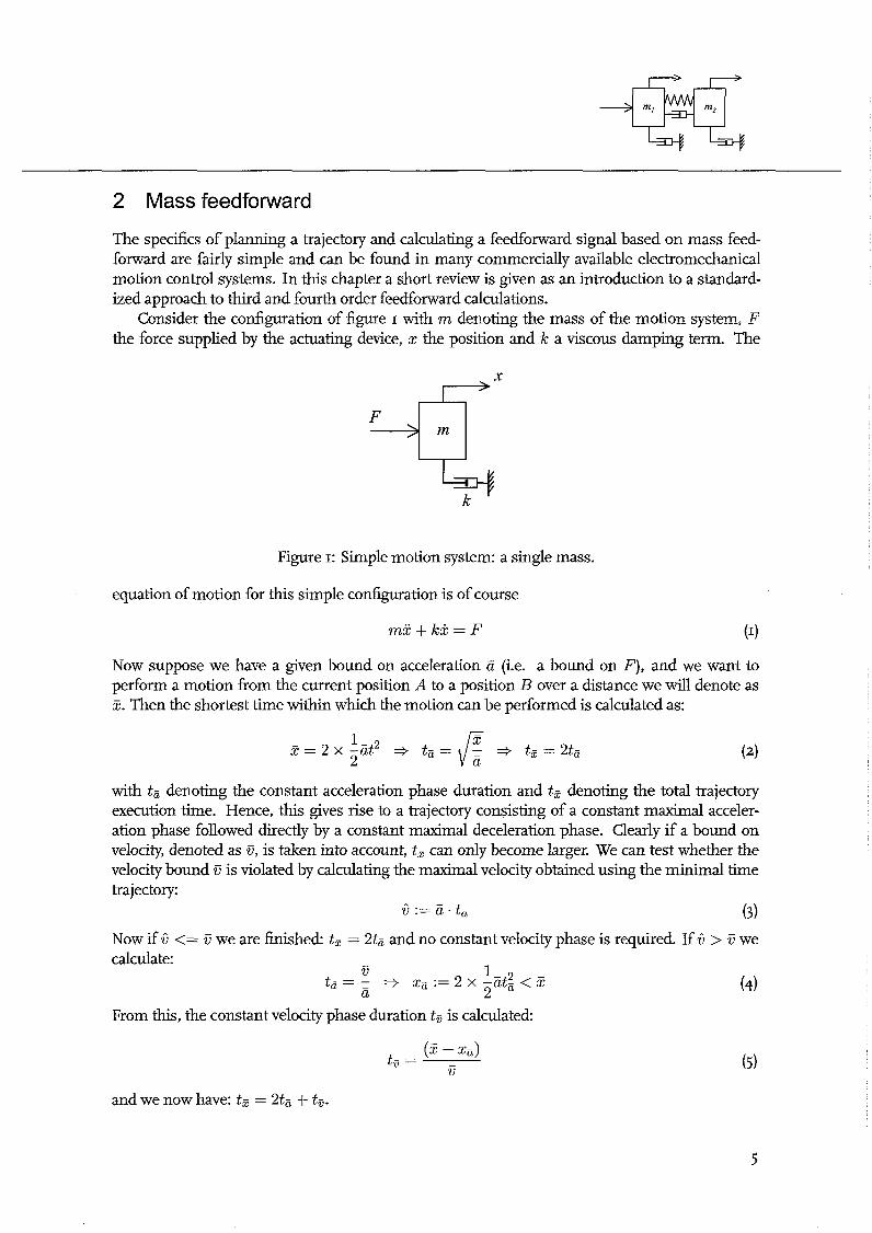
Comider the configuration of figure I with m denoting the mass of the motion system-, F the force supplied by the actuating device, x the position and k a viscous damping term. The
Figure I: Simple motion system: a single mass.
equation of motion for this simple configuration is of course
Now suppose we have a given bound on acceleration G (i-e. a bound on F), and we want to perform a motion from the current position A to a position B over a distance we will denote as 3. Then the shortest time within which the motion can be performed is calculated as:
with tzi denoting the constant acceleration phase duration and t , denoting the total trajectory execution time. Hence, this gives rise to a trajectory consisting of a constant maximal acceler- ation phase followed directly by a constant maximal deceleration phase. Clearly if a bound on velocity, denoted as u, is taken into account, t, can only become larger. We can test whether the velocity bound @ is violated by calculating the maximal velocity obtained using the minimal time trajectory:
A - v := a.t6 (3)
Now if 6 <= 8 we are finished: t , = 2t2 and no constant velocity phase is required. If 6 > B we calculate: -
v 1 tC = : .j zc := 2 x -3t: < z
a 2 (4)
From this, the constant velocity phase duration t , is calculated:
and we now have: t , = 2tG + t,.
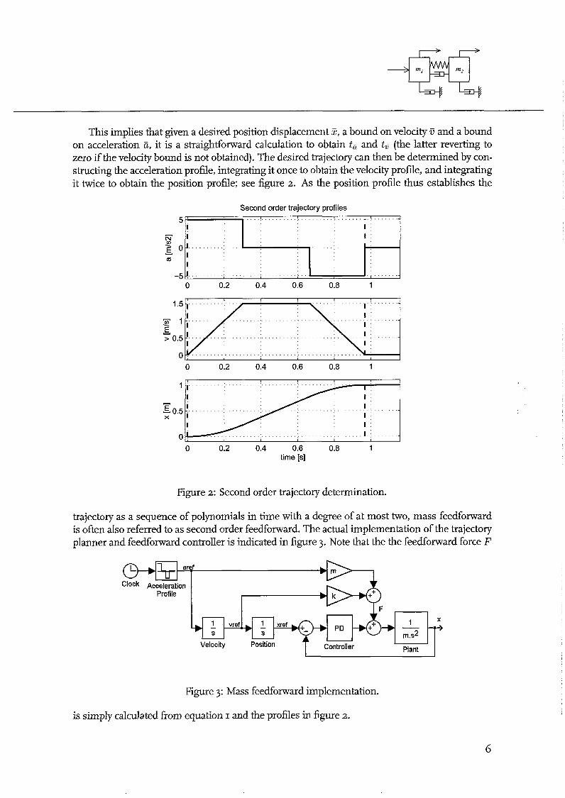
This implies that given a desired position displacement 3, a bound on velocity v and a bound on acceleration a, it is a straightforward calculation to obtain t, and tB (the latter reverting to zero if the velocity bound is not obtained). The desired trajectory can then be determined by con- structing the acceleration profile, integrating it once to obtain the velocity profile, and integrating it twice to obtain the position profile; see figure 2. As the position profile thus establishes the
Second order trajectory profiles
. . . . . . . . . . . . . . . . . .
m
0 0.2 0.4 0.6 0.8 1 time [s]
Figure 2: Second order trajectory determination.
trajectory as a sequence of polynomials in time with a degree of at most two, mass feedforward is often also referred to as second order feedforward. The actual implementation of the trajectory planner and feedforward controller is indicated in %re 3. Note that the the feedforward force F
Clock Acceleration Profile
Figure 3: Mass feedforward implementation.
is simply calculated fi-om equation I and the profiles in figure z.
1 PD -
m.s2
X
+
Velocity Position Controller Plant
3 Higher order feedforward
The previous chapter shows that mass feedforward is based on a simple single mass model of the motion system. This implies that the performance of mass feedforward is determined by how much the actual motion system deviates from this single mass model. On the other hand, the performance of the motion system as a whole is also determined by the quality of system compensation and/or feedback control. It can be stated that the success of feedback control is such that in many cases the mass feedforward approach is considered sufficient, given that an appropriate feedback controller is required anyway for disturbance reduction and stabilization.
However, when considering hrther improvement of motion control system performance, the use of hgher order feedforward is often a very effective approach in comparison with improved feedback control. The first effect is that higher order trajectories inherently have a lower energy content at higher frequencies, which results in a lower high frequency content of the error signal, which in turn enables the feedback controller to be more effective. The second effect is that h&er order trajectories have less chance of demanding a motion which is physically impossible to perform by the given motion system: e.g. most power amplifiers exhibit a 'rise time' effect, such that it is impossible to produce a step-like change in force.
These effects are commonly referred to as 'smoothing' and result in a decrease of positioning errors during execution of the trajectory and a reduced settling time. The disadvantage of higher order trajectories, i.e. the increase in trajectory execution time, is usually more than compensated by the reduced settling time. Because of this, many high performance motion systems are already equipped with a third order trajectory planner as a direct extension of mass feedforward. In this chapter it will be determined that a fourth order trajectory planner and feedforward calculation gives a significant further improvement.
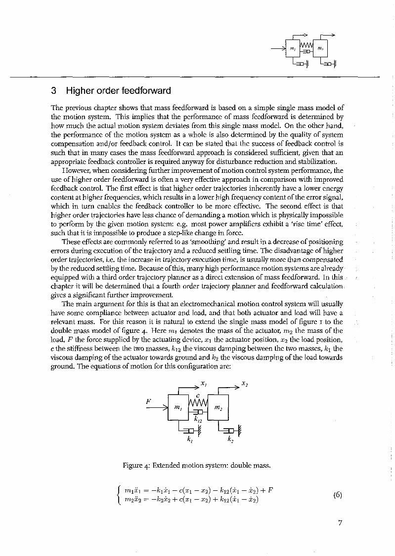
The main argument for this is that an electromechanical motion control system will usually have some compliance between actuator and load, and that both actuator and load will have a relevant mass. For this reason it is natural to extend the single mass model of figure I to the double mass model of figure 4. Here ml denotes the mass of the actuator, m2 the mass of the load, F the force supplied by the actuating device, xl the actuator position, x2 the load position, c the stiffness between the two masses, k12 the viscous damping between the two masses, kl the viscous damping of the actuator towards ground and k2 the viscous damping of the load towards ground, The equations of motion for this configuration are:
Figure 4: Extended motion system: double mass.
Laplace transformation and substitution then results in the following expression:
with:
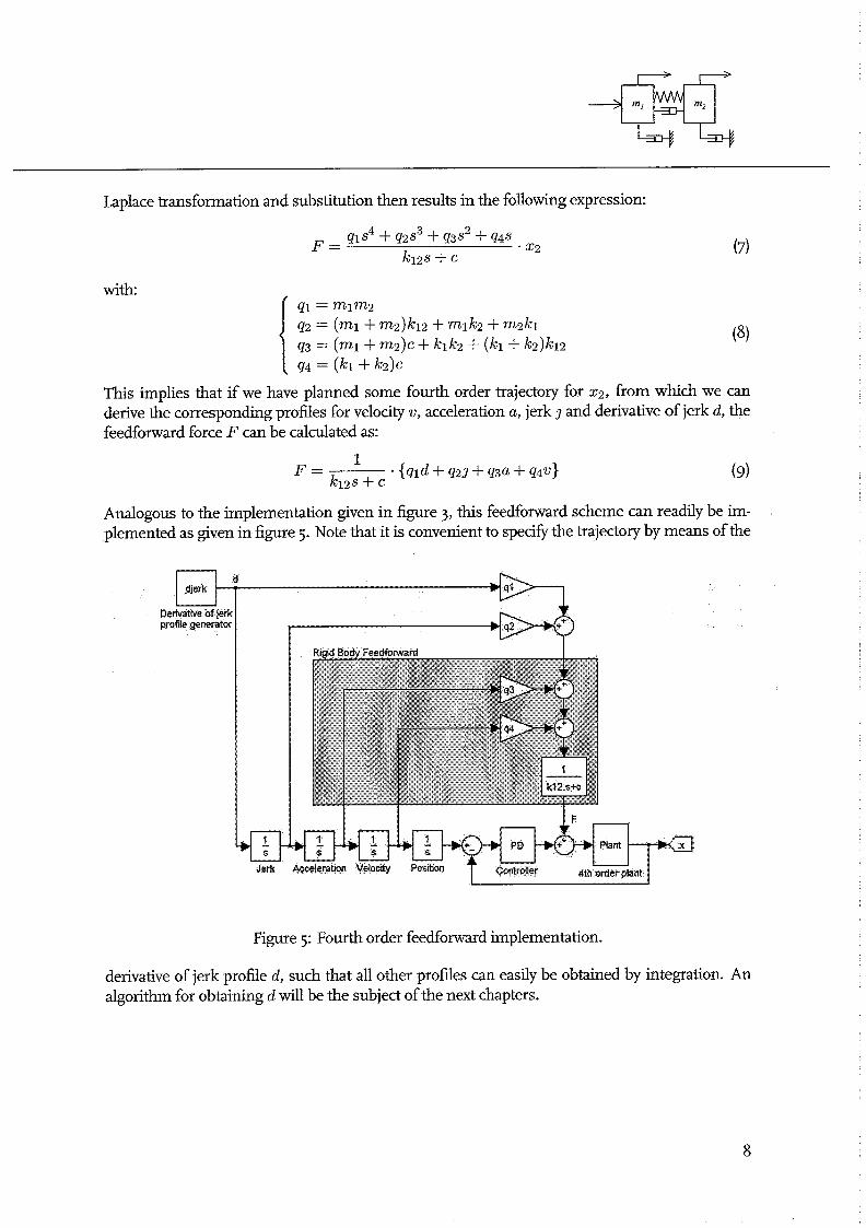
This implies that if we have planned some fourth order trajectory for x2, from which we can derive the correspondmg profiles for velocity v, acceleration a, jerk 2 and derivative of jerk d, the feedforward force F can be calculated as:
Analogous to the implementation given in figure 3, this feedforward scheme can readily be irn- plemented as given in figwe 5. Note that it is convenient to specify the trajectory by means of the
Figure 5: Fourth order feedforward implementation.
djerk
derivative of jerk profile d, such that all other profiles can easily be obtained by integration. An algorithm for obtaining d will be the subject of the next chapters.
d -
Dwivatiie of jerk profile generator
4 Higher order trajectory planning
Planners for second and third order trajectories are fairly well known in industry and academia and there are many approaches for obtaining a valid solution. Extension to fourth order trajectory planning is however not trivial. In this chapter we will review the main objectives of trajectory planning in general and set up an algorithm for obtaining these objectives more or less irrespec- tive of the order of the resdting trajectory.
As mentioned before, a trajectory is usually planned for a motion from the current position A to some desired end position B under some boundary constraints. This will also be the basis for the discussion given here, although the resulting algorithm can be adjusted for relevant alter- native objectives like for instance speed control instead of position control, scanning motions or speed change operations. Several fwther objectives that are of importance for applicability of a trajectory planning algorithm ar given below.
e Timing. In principle we should strive for time optimality; at least it must be clear what the consequences are for the trajectory execution time when considering the effect of boundary conditions.
Actuator effort. This is usually the basis for the selection of bounds for velocity, acceleration and jerk, although they may also be related to bounds on mechanics or safety issues.
Accuracy. For point to point moves, the planned end position of the trajectory must be equal to the desired end position (within measurement accuracy).
Complexity. Usually trajectory planning is thought of as being done off-line. In practice however, the desired end position often becomes available at the moment the trajectory should start. Hence, the time required for planning the trajectory is lost and should be minimized.
Reliability. The planning algorithm should always come up with a valid solution.
Implementation. Trajectory planning is done in computer hardware, and is therefore sub- ject to discretization and dgttization.
Now we argue that these objectives, except the final one, are all met by the simple algorithm given in chapter 2 (slightly adjusted):
I. calculate t , from equation 2,
2. calculate .fi from equation 3,
3. test 6 > G:
if true calculate t, from equation 4,
iffalse set t, = it,,
4. calculate x, from equation 4,
5. calculate t, from equation 5, and
6. finished: t, and to completely determine the trajectory.
First consider timing; obviously timing is minimal if the bound on v is discarded as is done in step I. If introducing this bound leads to a reduction oft, (verify that equation 4 always leads to a reduction) the result will be that v = is obtained in the shortest possible time, and is continued for as long as possible. Hence the trajectory execution time is always minimal, given the bounds a and @. Next, actuator effort is immediately taken into account by means of the given bounds, accaacy is precise, complexity is very low and reliability is high (no iteration loops thzt can hang up, algorithm only fails if a non-positive bound is specified). The implementation problem is considered later.
Given the advantages of this algorithm, it is desirable to generalize it for planning higher order trajectories. The position displacement 3 and bounds on all derivatives of the trajectory up to the highest order derivative d (indicated as d) are assumed to be given. Furthermore we will require that all derivatives are equal to zero at the start and end positions.
I. Determine a symmetrical trajectory that has d equal to either d or -d at all times and obtains displacement 3.
2. Determine td: the shortest time that d remains constant (always the first period).
3. Calculate the maximal value of velocity 5 obtained during this trajectory.
a if true re-calculate td based on v (td decreases),
a if false continue.
5. Calculate the maximal value of acceleration ti obtained during this trajectory.
6. Test ti > a:
a iftrue re-calculate td based on a (td decreases),
if false continue.
7. Continue these tests and possible recalculations until d; the last test is performed on j, defined as the h&est derivative before d. The resulting td will not be changed anymore.
8. Extend the trajectory symmetrically with periods of constant j whenever j reaches the value 3 or -j? this must be done such that the required displacement 3 is obtained.
g. Determine t,-: the shortest time that j remains constant.
10. Starting with velocity and ending with the derivative before j, calculate the maximal value and re-calculate t,- if the appropriate bound is violated (each re-calculation can only decrease t?).
11. The resulting t,- will not be Changed anymore.
12. Extend the trajectory symmetrically with periods of constant next lower derivative; again such that the required displacement 3 is obtained. Determine the associated time interval and do the tests and recalculations resulting in a h a 1 value for it.
13. Continue until v: the constant speed phase duration t , is calculated such that the required displacement 3 is obtained (i.e. the displacement 'left to go' divided by v).
14. Finished: t ~ , t3, etc. until tv completely determine the trajectory.
The properties of the resulting trajectories (in the sense of the objectives given above) appear to depend partly on the order of the trajectory planner. Obviously, the required calculations be- come more complex with increasing order. Time-optimality is still automatically obtained with third order trajectories, but not necessarily for fourth order trajectories (this can be obtained but costs much complexity at a small gain with respect to a good sub-optimal solution). In principle, higher than fourth order trajectories can also be planned by means of this algorithm, but this is considered impractical due to the large increase in complexity. It is noted here that all calculations for third and fourth order planning can be done analytically with fairly basic mathematical func- tions, except one calculation for fourth order planning. For this case a simple and numerically stable search algorithm can be used.
The next chapter will provide the calculations for third order trajectory planning; after that fourth order trajectory planning will be considered.
5 Third order trajectory planning
Although chapter 3 shows that fourth order trajectory planning and feedfonvard is strongly mo- tivated by a model based approach, it may still be useful to apply third order trajectory planning. This chapter will provide the derivations and calculations necessary to 'fill in' the algorithm de- veloped in chapter 4 for third order trajectory planning. We will assume that a trajectory must be planned over a distance 3, that bounds are given on velocity (a), acceleration (8) and jerk (2, and that the trajectory must be time optimal within these bounds. The bound on jerk can for instance be related to 'rise time7 behavior as commonly found in electromechanical actuation sys- tems with a non-ideal power amplser for generating the actuation force. This results in a bound on the maximal current change per second, which translates to a maximal actuation force change per second and a maximal acceleration change per second: hence a bound on jerk.
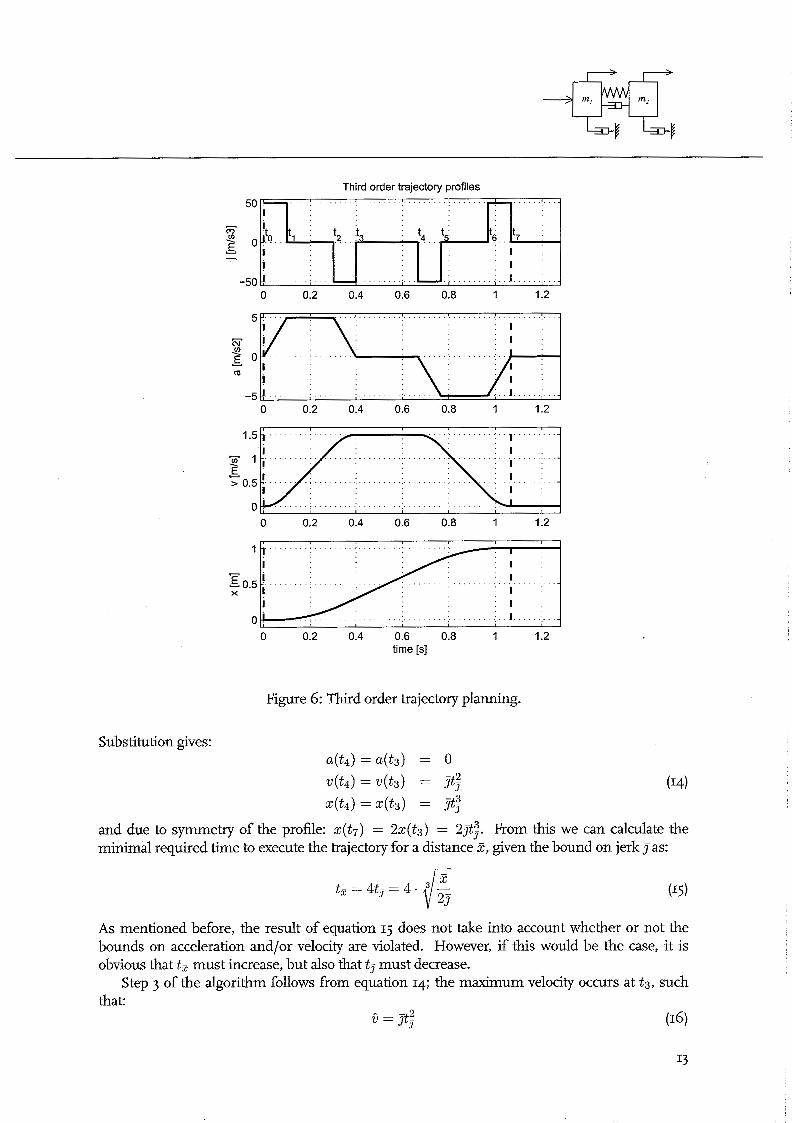
The trajectory planning algorithm will be based on the construction of an appropriate jerk profile (instead of the acceleration profile as in mass feedfonvard) that can be integrated three times to obtain the third order position trajectory. A symmetrical trajectory is completely deter- mined by three time intervals: the constant jerk interval t,-, the constant acceleration interval ti, and the constant velocity interval t,. The resulting profiles are given in figure 6. Including the starting time of the trajectory at to, there are eight time instances at which the jerk changes. The following relations are dear:
For step I of the algorithm, we will discard the bounds on acceleration and velocity, and only consider the bound on jerk. This implies t, = 0 and t6 = 0 and it is dear that this will provide us with a lower bound for the trajectory execution time t , = 4 x t,-.
To obtain t,- (step 21, we need the relation between t,- and Z with given 3: For this we make use of the constant value of jerk of +? or -J during each interval. If we set the time instance of jerk change to o, it is easily verified that for any time t during the constant jerk interval the third order profiles for acceleration, velocity and position can be expressed as follows:
Because we assume that the bounds on acceleration and velocity are not violated, we have ti, = 0 and t, = 0, and consequently from figure 6: t2 = tl = t,- and t4 = t3. Hence:
and for the next period in which 3 = -3
Third order trajectory profiles
time [s]
Figure 6: Third order trajectory planning.
Substitution gives:
and due to symmetry of the profile: x(t7) = 2x(t3) = 23%;. From this we can calculate the minimal required time to execute the trajectory for a distance 2 given the bound on jerk j as:
As mentioned before, the result of equation 15 does not take into account whether or not the bounds on acceleration and/or veloaty are violated. However, if this would be the case, it is obvious that t, must increase, but also that t,- must decrease.
Step 3 of the algorithm follows from equation 14; the maximum velocity ocms at t3, such that:
6 = jt; (16)
If 6 > ij the bound is violated and we must recalculate t,- as follows:
Note that the resulting t,- will always be smaller than the result from equation 15, and that conse- q~ently also the acceleration (from equation 12) will become smaller. This establishes step 4 of the algorithm.
Step 5 follows from equation 12; the maximum acceleration occurs at tl, such that:
If 6 > a the bound is violated and we must recalculate t,- as follows:
Again t,- can only be smaller than previously calculated, such that we now have the guarantee that t,- is the maximal value for which none of the bounds is violated. At the same time we have that a maximal value oft,- will lead to a minimal value oft, and will therefore be (part of) the time- optimal solution. This establishes step G of the algorithm and because a is the highest derivative before j, also step 7.
The next thing to do is to calculate t,: also this value should be maximal for time-optimal performance, while at the same time it must be such that no bounds are violated. To do the necessary calculations, assume that tG > 0, such that we now have t2 > tl (from figure 6). Equation 12 can then be extended with the help of equation 11 and the fact that 3 = 0 during the period from tl to t2:
Now we assume that the velocity bound is not violated, such that t4 = ts. Then due to symmetry of the profile we have:
3 2 x (t7) = 2x (t3) = 2Jtf + 3jt;ta + s t , (22)
By setting z = z(t7) we can then solve tZ from the following:
As t , must be positive to make sense, the solution is:
Note that t , >= 0 follows immediately from 17: >= 2Jt;. Hence, we now have determined t , under the assumption that the velocity bound will not be violated: equation 24 establishes steps 8 and g of the algorithm.
Step 10 introduces the velocity bound again; the maximal velocity is obtained at t3 (see 21):
If 6 > ij the bound is violated and we can recalculate ta as follows:
Now we have determined t7 and t, to be the time-optimal solution under the restriction of the given bounds (step 11).
As the next lower derivative is already v, we can skip step 12 and continue with step 13: the determination of the constant velocity time interval t, such that the required total displacement 3 is obtained. From the previous calculations follows that ts = 0 if t, is according to equation w. But if t , is reduced accordmg to equation 26, we will have x(t7) < 17: and we must add a constant velocity phase to the trajectory such that x(t4) - x(t3) = 17: - 22 (t3). With equation 21 this implies that we can calculate t , as:
17: - 27t; - 37t;t, - Jt& t, = -
v This completes the calculation of the characteristics of the time-optimal third order profile for a given distance 3 and given bounds ij, ii and 7. The total displacement 3 can be expressed as a function of 7 and the times t,-, t , and t6:
6 Fourth order trajectory planning
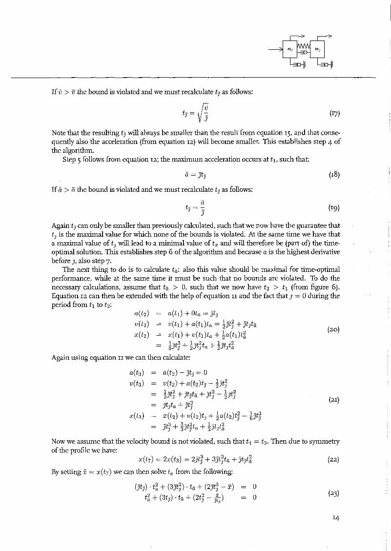
This chapter will provide the derivations and calculations necessary to 'fill in' the algorithm devel- oped in chapter 4 for fourth order trajectory planning. Again we will assume that a symmetrical trajectory must be planned for a point to point move over a &stance Z. We have bounds on veloc- ity (v), acceleration (ii), jerk (3 and derivative of jerk (d). The trajectory planning algorithm will now be based on the constmction of a derivative of jerk profile that can be integrated four times to obtain the fowth order position trajectory. A symmetrical trajectory is completely determined by four time intervals: the constant derivative of jerk interval t d ; the constant jerk interval tJ, the constant acceleration interval t, and the constant velocity interval tG. The resulting profiles are given in figure 7. Including the starting time of the trajectory at to, there are sixteen time
instances at which the derivative of jerk changes. For step I of the algorithm, we will discard the bounds on jerk, acceleration and velocity, and
only consider the bound on the derivative of jerk. This implies tG = 0, t , = 0 and t,- = 0 and it is clear that this will provide us with a lower bound for the trajectory execution time t, = 8 x t&
To obtain t d (step 2), we need the relation between t d and z with given d. For this we make use of the constant value of derivative of jerk of +d or -d during each interval. If we set the time instance oI' derivative of jerk change to o, it is easily ve~;fied that for any b e t during the constant derivative of jerk interval the fourth order profiles for acceleration, velocity and position can be expressed as follows:
3 ( t ) = d o t + jo a ( t ) = $dot2 + j o t + a0
v ( t ) = i d o t 3 + ; jot2 + a o t + v o (29)
x ( t ) = &dot4 + i 3 0 t 3 + a o t 2 + v o t + x o
Because we assume that the bounds on jerk, acceleration and velocity are not violated, we have t,- = 0, t, = 0 and t, = 0, and consequently from figure 7: t2 = tl = td; t 4 = t3 = 2td, t6 = t5 = 3td and t s = t7 = 4t,-. Hence:
and for the next period in which d = -2:
Substitution gives: j ( t 3 ) = 0
Again using equation 29, we can calculate the results of the subsequent periods as:
and:
and due to symmetry of the profile: x(t 15) = 22 (t7) = 8dt$ From this we can calculate td as required by steps I and 2 of the trajectory planning algorithm as:
To continue with step 3 we have that the maximal velocity is obtained at time instance t7. Hence, from equation 34 follows:
- 3 8 = ~ ( t 7 ) = 2dtd
If 6 > E we must recalculate td as: r
which establishes step 4. Next, step 5 follows from the calculation of maximal acceleration ob- tained at time instance t3. From equation 32 we have:
and if 6 > a we must recalculate td as:
t d = g which establishes step 6. In this case we have one further test (step 7) to do on the maximal jerk obtained at t 1 : -
j = 3(tl) = dtd (40)
and if j > 3 we must recalculate td as: - 3
t" 2 Hence, we now have a value for t l that complies with all of the bounds 3 a and G.
The next thing to do is to calculate t,- under the assumption that bounds a and 8 are not violated (steps 8 and 9). To do the necessary calculations, assume that t,- > 0, such that we now have t2 > tl and t6 > t5 (from figure 7). Equation 29 and the fact that d = 0 during the period from tl to t2 now enables us to calculate:
Again using equation 29 we can then calculate:
Now with t8 = t7 and due to symmetry of the profile we have:
By setting I = x(t15) we can then solve tT from the following:
As this is a third order polynomial in t,- there is no analytical solution available. However, we are looking for a positive real solution of a polynomial with positive coefficients except the final one. This implies that we can set up a simple and well-defined numerical search to find the solution.
After this, step 10 introduces the velocity and acceleration bounds again; the maximal velocity is obtained at t7 (see 46):
6 = v(t7) = 2dti + + dt& (49)
If 6 > . the bound is violated and we can recalculate t,- from the second order polynomial:
The positive real solution for this is:
Next, the maximal acceleration is obtained at t~ (see 43):
If li > G we can recalculate t,- as: - a t - - - - t -
J - J d (53)
and we arrive at step 11 of the planning algorithm. In accordance with step 12 there is one further extension of the trajedory required for the
calculation oft,. To do the necessary calculations, assume that tC > 0, such that we now have
t4 > t3 (from figure 7). Equation 29 and the fact that d = 0 and j = 0 during the period from t3 to t4 now enables us to calculate:
Now, given that td and t7 are already determined and the planned trajectory is symmetrical, we can solve t , such that x (t = 2x (t7) = 3 from the following polynomial equation:
Clearly t, must be the positive root of this second order polynomial (compare with equation 24). Now we can introduce the velocity bound again; the maximal velocity is obtained at t7 (see
If 6 > the bound is violated and we can recalculate t , as:
Now we have determined td; t,- and tT, under the restriction of the given bounds and, as the next derivative is v, this establishes step 12 of the algorithm.
Finally, step 13 will determine the constant velocity time interval t, such that the required total displacement 3 is obtained. From the previous calculations follows that tG = 0 if t, is according to equation 58. But if tT, is reduced according to equation 60, we will have x( t I5 ) < 3 and we must add a constant velocity phase to the trajectory such that x(t4) - x( tg ) = J: - 2x(t7). With equation 57 this -hplies that we cafi calculate tG as:
This completes the calculation of the characteristics of the symmetrical fourth order profile for a given distance and given bounds v, zi, and d. We can M e r state that if the trajectory contains a constant velocity phase (i.e. t, > O), the trajectory is time-optimal. The total displacement J: can be expressed as a function of d and the times ta tJ, t6 and t,:
7 Implementation aspects
7.1 Switching times
From the previous chapters it is clear that the derivations for especially fourth order trajectory planning are quite elaborate. However, the calculations actually required for implementation of this planner are relatively straightforward. The algorithm of chapter 4 consists of a combination of polynomial calculations with simple if-then-else tests for which most state-of-the-art motion control hardware has standard algorithms.
When considering implementation of the planned trajectory into a feedforward control scheme, it is important to consider the effect of discretization. This implies that the integrators and the feedforward filter as given in the diagram of figure 5 will all have to be implemented in discrete time at some given sampling time interval Ts. This also implies that the switching time instances of the planned trajectory must be synchronized with the sampling time instances: i.e. the time intervals t,, th, etc. must be multiples of Ts-
To obtain this, it must be accepted that time-optimality as resulting from the continuous time calculations in the previous chapters is lost. The calculated time intervals must be rounded-off towards a multiple of T,. This must be done such that the given bounds are not violated, but at the same time approximated as closely as possible. The approach proposed here is to extend the algorithm of chapter 4. After each calculation or re-calculation of a time interval, the result is rounded-off upward to the next multiple of Ts- Next the maximal value of the highest derivative is calculated accordingly.
As an example consider the first calculation of td for a fourth order trajectory (equation 35). The rounded-off value for td can be calculated as:
with ceil(.) denoting the rounding off towards the next higher integer, From equation 35 we can then calculate a new value for d -
Note that with t i 2 ta we must have d 5 l. It can be verified that this same approach is valid for the calculation or re-calculation of all
time intervals. It is important to note that with each new calculation of d its value must reduce. This guarantees that none of the bounds that were checked in earlier steps of the algorithm will be violated.
State-of-the-art motion controllers are equipped with a high resolution floating point calculation unit, such that quantization effects are usually negligible. To check this, we can make use of equa- tion 62 to calculate the obtained position in case a quantized 2 is used. The difference between desired position and calculated position can be accounted for by means of a correction signal on the position trajectory. Typically in a digital system, the position signal is also quantized (usually in encoder increments). The correction signal can then be implemented by adding some incre- ments to the position reference at each sampling instance during the trajectory. In relevant cases only one or two correction increments at each sampling instance should be sufficient (to prevent deterioration of the feedforward control). In case larger corrections are necessary, the accuracy and/or sampling rate of the motion control hardware should be increased.
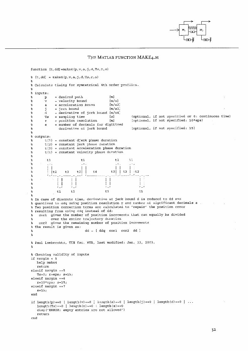
A complete algorithm for fourth order trajectory planning is given in the appendix. This algo- rithm is given as a Matlab .M function, which calculates the times td t?, t, and t,. It also includes the possibility to specify a sampling time interval. It then uses equations 63 and 64 to synchro- nize the switching time instances with the sampling time instances and to calculate 2''. Finally, it allows compensation for the effect of quantization by specifjmg a number of significant decimals for 2 and calculating the required amount of correction increments for the position reference sig- nal.
7.2 Synchronization of profiles
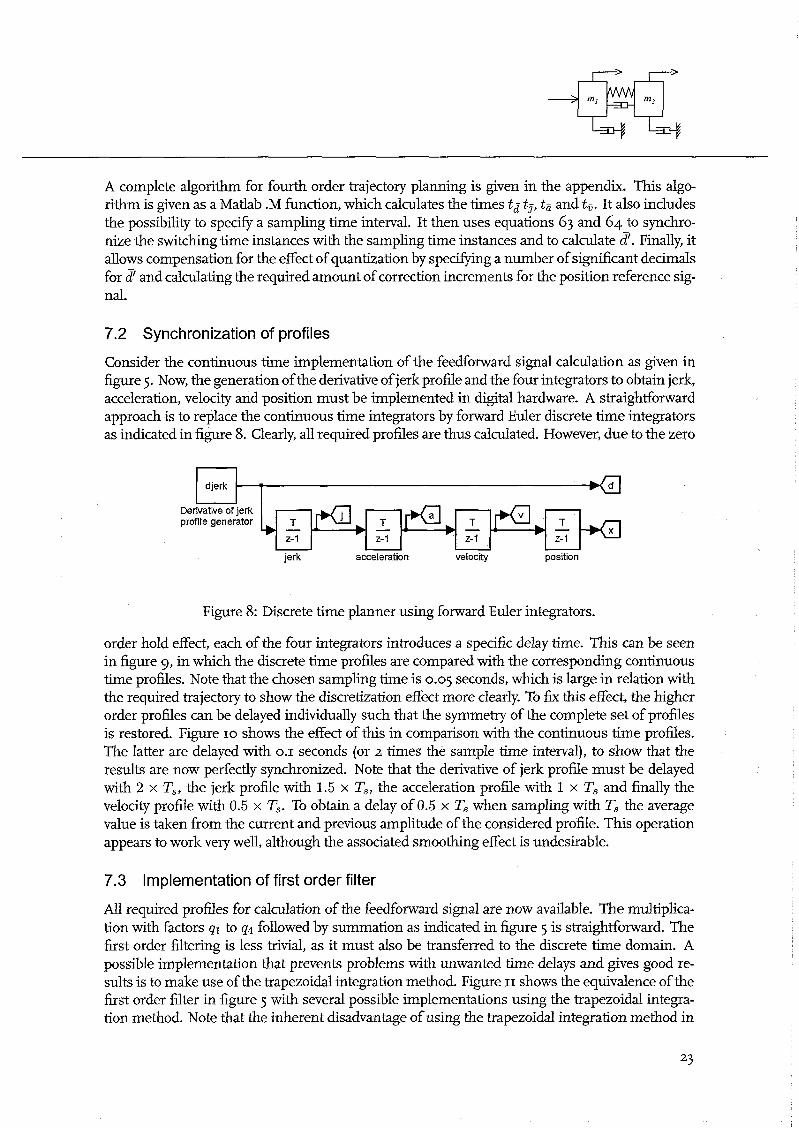
Consider the continuous time implementation of the feedforward signal calculation as given in figure 5. Now, the generation of the derivative of jerk profile and the four integrators to obtain jerk, acceleration, velocity and position must be implemented in digital hardware. A straightforward approach is to replace the continuous time integrators by forward Euler discrete time integrators as indicated in figure 8. Clearly, all required profiles are thus calculated. However, due to the zero
I djerk
jerk acceleration velocity position
1 - Derivaf~e of jerk profile generator
Figure 8: Discrete time planner using forward Euler integrators.
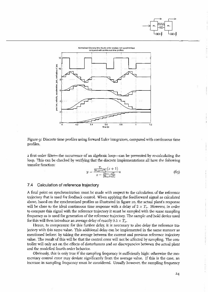
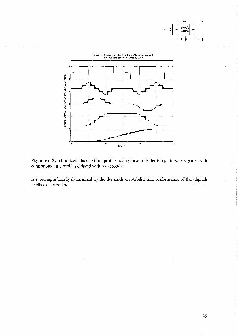
order hold effect, each of the four integrators introduces a specific delay time. This can be seen in figure g, in which the discrete time profiles are compared with the corresponding continuous time profiles. Note that the chosen sampling time is 0.05 seconds, which is large in relation with the required trajectory to show the discretization effect more clearly. To fix this effect, the higher order profiles can be delayed individually such that the symmetry of the complete set of profiles is restored. Figure 10 shows the effect of this in comparison with the continuous time profiles. The latter are delayed with 0.1 seconds (or 2 times the sample time interval), to show that the results are now perfectly synchronized. Note that the derivative of jerk profile must be delayed with 2 x T,, the jerk profile with 1.5 x Ts? the acceleration profile with 1 x T, and finally the velocity profile with 0.5 x Ts. To obtain a delay of 0.5 x Ts when sampling with Ts the average value is taken from the current and previous amplitude of the considered profile. This operation appears to work very well, although the associated smoothing effect is undesirable.
T -
7.3 Implementation of first order filter
-, z-1
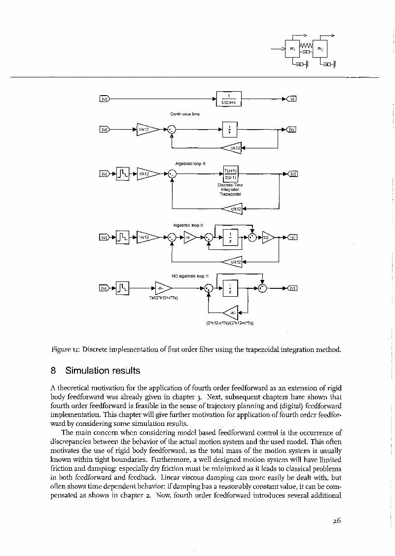
All required profiles for calculation of the feedforward signal are now available. The multiplica- tion with factors ql to q4 followed by summation as indicated in figure 5; is straighi50rward. The first order filtering is less trivial, as it must also be transferred to the discrete time domain. A possible implementation that prevents problems with unwanted time delays and gives good re- sults is to make use of the trapezoidal integration method. Figure 11 shows the equivalence of the first order filter in figure 5 with several possible implementations using the trapezoidal integra- tion method. Note that the inherent disadvantage of using the trapezoidal integration method in
z-1
T - T
Normalized Discrete time fourth order profiles: not synchronized compared with continuous time profiles
" 0 0.2 0.4 0.6 0.8 1 1.2 time [s]
Figure g: Discrete time profiles using forward Euler integrators, compared with continuous time profiles.
a first order filter-the occurrence of an algebraic loop-can be prevented by re-calculating the loop. This can be checked by verifjmg that the discrete implementations all have the following transfer function: -
7.4 Calculation of reference trajectory
A final point on synchronization must be made with respect to the calculation of the reference trajectory that is used for feedback control. When applying the feedforward signal as calculated above, based on the synchronized profiles as illustrated in figure 10, the actual plant's response will be close to the ideal continuous time response with a delay of 2 x T,. However, in order to compare this signal with the reference trajectory it must be sampled with the same sampling frequency as is used for generation of the reference trajectory. The sample and hold device used for this will then introduce an average delay of exactly 0.5 x T,.
Hence, to compensate for this further delay, it is necessary to also delay the reference tra- jectory with this same value. This additional delay can be implemented in the same manner as mentioned before: by taking the average between the current and previous reference trajectory value. The result of this will be that the control error will not be affected by sampling. The con- troller will only act on the effects of &sturbances and on discrepancies between the actual plant and the modelled fourth order behavior.
Obviously, this is only true if the sampling frequency is sufficiently high: otherwise the mo- mentary control error may deviate significantly from the average value. If this is the case, an increase in sampling frequency must be considered. Usually however, the sampling frequency
Normalized Discrete time fourth order profiles: synchronized continuous time profiles delayed by 0.1 s
time [s]
Figure 10: Synchronized discrete time profiles using forward Euler integrators, compared with coniinuous time profiles delayed with 0.1 seconds.
is more significantly determined by the demands on stability and performance of the (digital) feedback controller.
Continuous time
Integrator: Trapezoidal I
Algebraic loop !! -
Algebraic loop !! I I
,
NO alaebralc looo !!
T(z+l) 2(Z-1) -
Figure 11: Discrete implementation of first order filter using the trapezoidal integration method.
Discrete-Time
8 Simulation results
A theoretical motivation for the application of fourth order feedforward as an extension of rigid body feedforward was already given in chapter 3. Next, subsequent chapters have shown that fourth order feedforward is feasible in the sense of trajectory planning and (digital) feedforward implementation. This chapter will give fwther motivation for application of fourth order feedfor- ward by considering some simulation results.
The main concern when considering model based feedforward control is the occurrence of discrepancies between the behavior of the actual motion system and the used model. This often motivates the use of rigid body feedforward, as the total mass of the motion system is usually known within tight boundaries. Furthermore, a well designed motion system will have limited friction and damping: especially dry friction must be minimized as it leads to classical problems in both feedforward and feedback. Linear viscous damping can more easily be dealt with, but often shows time dependent behavior: if damping has a reasonably constant value, it can be com- pensated as shown in chapter 2. Now, fourth order feedforward introduces several additional
Table I: Simulation parameters
Variation ml E (15.. .25), m2 = 30-ml k l ~ { 5 . - . 1 5 ) , k2 = 20 - kl
=t 33% =tIOO%
Parameter ml m2 h k2
c!
k12
Table 2: Trajectory definition parameters
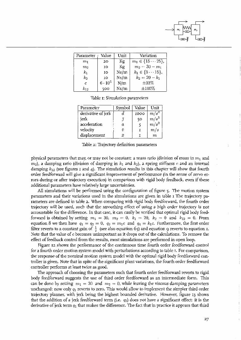
physical parameters that may, or may not be constant: a mass ratio (division of mass in ml and m2), a damping ratio (division of damping in kl and k2), a spring stiffness c and an internal damping k12 (see figures I and 4). The simulation results in this chapter will show that fourth order feedforward will give a significant improvement of performance (in the sense of servo er- rors during or after trajectory execution) in comparison with rigid body feedback, even if these additional parameters have relatively large uncertainties.
All simulations will be performed using the configuration of figure 5. The motion system parameters and their variations used in the simulations are given in table I The trajectory pa- rameters are defined in table 2. When comparing with rigid body feedforward, the fourth order trajectory will be used, such that the smoothing effect of using a high order trajectory is not accountable for the difference. In that case, it can easily be verified that optimal rigid body feed- forward is obtained by setting ml = 30, mg = 0, kl = 20, k2 = 0 and k12 = 0. From equation 8 we then have ql = qg = 0, q3 = mlc and qq = klc. Furthermore, the first order filter reverts to a constant gain of $ (see also equation 65) and equation g reverts to equation I. Note that the value of c becomes unimportant as it drops out of the calculations. To remove the effect of feedback control from the results, most simulations are performed in open loop.
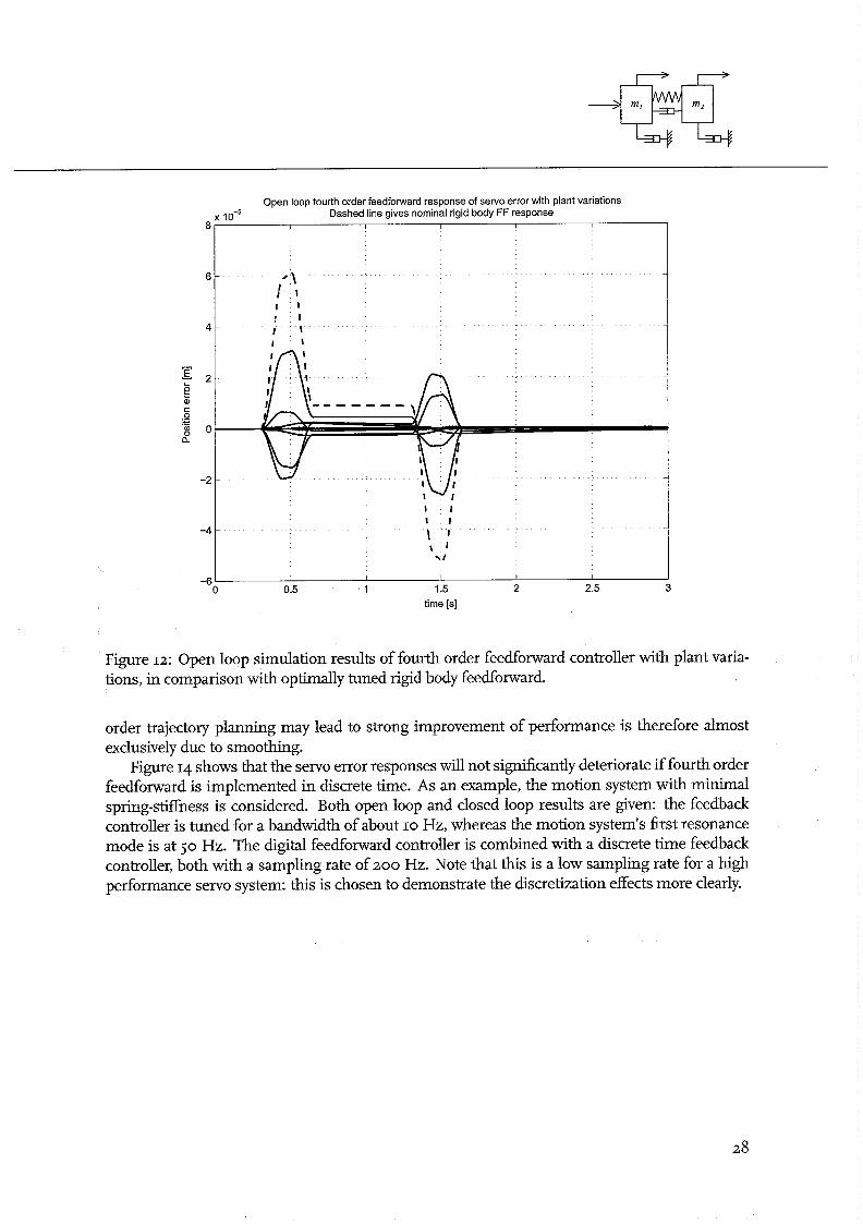
Figure 12 shows the performance of the continuous time fourth order feedforward control for a fourth order motion system model with perturbations according to table I. For comparison, the response of the nominal motion system model with the optimal rigid body feedforward con- troller is given. Note that in spite of the significant plant variations, the fourth order feedforward controller performs at least twice as good.
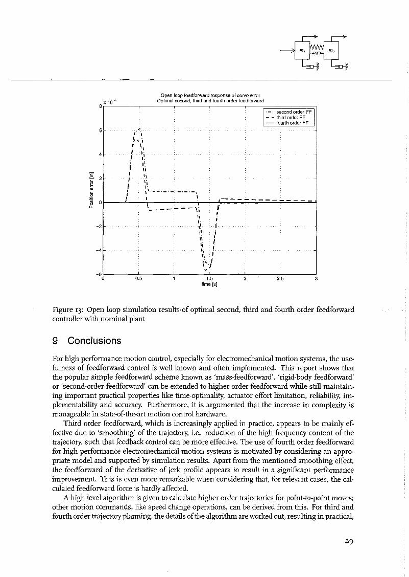
The approach of choosing the parameters such that fourth order feedforward reverts to rigid body feedforward suggests the use of third order feedforward as an intermediate form. This can be done by setting ml = 30 and m2 = 0, while leaving the viscous damping parameters unchanged: now only ql reverts to zero. This would allow to implement the simpler third order trajectory planner, with jerk being the highest bounded derivative. However, figure 13 shows that the addition of a jerk feedforward term (i-e. q2) does not have a significant effect: it is the derivative of jerk term ql that makes the difference. The fact that in practice it appears that third
Value 20
10
10
10
6 . 1 0 ~ ~ o o
Unit m/s4 m/s3 m/s2 m/s m
Parameter derivative of jerk jerk acceleration velocity displacement
Unit Kg I@
Ns/m Ns/m ~ / m Ns/m
Symbol d
7 - a - v - x
Value 1000
50
5 I
I
-6l I I I I I I
0 0.5 1 1.5 2 2.5 3 time [s]
Open loop fourth order feedforward response of servo error with plant vanations x 1 o - ~ Dashed line gives nominal rigid body FF response
Figure 12: Open loop simulation results of fourth order feedforward controller with plant varia- tions, in comparison with optimally tuned rigid body feedforward.
8
6
4
order trajectory planning may lead to strong improvement of performance is therefore almost exclusively due to smoothing.
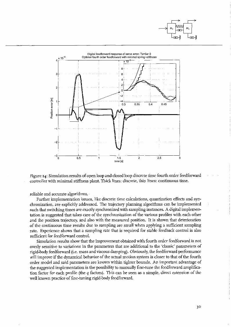
Figure 14 shows that the servo error responses will not significantly deteriorate if fourth order feedforward is implemented in discrete time. As an example, the motion system with minimal spring-stifhess is considered. Both open loop and closed loop results are given: the feedback controller is tuned for a bandwidth of about 10 Hz, whereas the motion system's first resonance mode is at 50 Hz. The digital feedforward controller is combined with a discrete time feedback controller, both with a sampling rate of 200 Hz. Note that this is a low sampling rate for a high performance servo system: this is chosen to demonstrate the discretization effects more clearly.
4 I I I I
- * \ /
I I I
- 1 1
"0 0.5 1 1.5 2 2.5 3 time [s]
Open loop feedforward response of servo error x lo'= Opt~rnal second, thrd and fourth order feedforward
Figure 13: Open loop simulation results of optimal second, third and fourth order feedforward controller with nominal plant
8
6
9 Conclusions
I I I I I
- . second order FF - - third order FF - fourth order FF - . *. -
I \
For high performance motion control, especially for electromechanical motion systems, the use- fulness of feedforward control is well known and often implemented. This report shows that the popular simple feedforward scheme known as 'mass-feedforward', 'rigid-body feedforward' or 'second-order feedforward' can be extended to higher order feedforward while still maintain- ing important practical properties like time-optimality, actuator effort limitation, reliability, im- plementability and accuracy. Furthermore, it is argumented that the increase in complexity is manageable in state-of-the-art motion control hardware.
Third order feedforward, which is increasingly applied in practice, appears to be mainly ef- fective due to 'smoothing' of the trajectory, i.e. reduction of the high frequency content of the trajectory, such that feedback control can be more effective. The use of fourth order feedforward for high performance electromechanical motion systems is motivated by considering an appro- priate model and supported by simulation results. Apart from the mentioned smoothing effect, the feedforward of the derivative of jerk profile appears to result in a significant performance improvement. This is even more remarkable when considering that, for relevant cases, the cal- culated feedforward force is hardly affected.
A high level algorithm is given to calculate higher order trajectories for point-to-point moves; other motion commands, like speed change operations, can be derived from this. For third and fourth order trajectory planning, the details of the algorithm are worked out, resulting in practical,
Digital feedforward response of servo error: Ts=5e-3
x lo-5 Optimal fourth order feedforward with minimal spring-stiffness 4 I I
I X l O ' I I I
-31 I I I I I I 0 0.5 1 1.5 2 2.5 3
time [s]
Figure 14: Simulation results of open loop and closed loop discrete time fourth order feedforward controller with minimal stiffness plant. Thick lines: discrete, thin lines: continuous time.
reliable and accurate algorithms. Further implementation issues, like discrete time calculations, quantization effects and syn-
chronization, are explicitly addressed. The trajectory planning algorithms can be implemented such that switching times are exactly synchronized with sampling instances. A digital implemen- tation is suggested that takes care of the synchronization of the various profiles with each other and the position trajectory, and also with the measured position. It is shown that deterioration of the continuous time results due to sampling are small when applying a sufficient sampling rate. Experience shows that a sampling rate that is required for stable feedback control is also sufficient for feedforward control.
Simulation results show that the improvement obtained with fourth order feedforward is not overly sensitive to variations in the parameters that are additional to the 'dassic' parameters of rigid-body feedforward (i.e. mass and viscous damping). Obviously, the feedforward performance will improve if the dynarnical behavior of the actual motion system is closer to that of the fourth order model and said parameters are known within W t e r bounds. An important advantage of the suggested implementation is the possibility to manually fine-tune the feedforward amplifica- tion factor for each profile (the q factors). This can be seen as a simple, direct extension of the well known practice of fine-tuning rigid-body feedforward.
References
[I] M. Boerlage, M. Steinbuch, P. Larnbrechts, M. van de Wal, 'Model based feedforward for motion systems'. Submitted, 2003.
[2] S. Devasia, 'Robust inversionbased feedforward controllers for output tracking under plant uncertainty'. Proc. of the American Control Conference, 2000, pp.qg7-502.
[3] B.G. Dijkstra, N.J. Rambaratsingh, C. Scherer, O.H. Bosgra, M. Steinbuch, S. Kerssemakers, 'Input design for optimal discrete-time point-to-point motion of an industrial XY positioning table', in Proc. 39th IEEE Conference on Decision and Control, 2000, pp.901-906.
[4] L. Hunt, G. Meyer, 'Noncausal inverses for linear systems'. IEEE Trans. on Automatic Control, 1996, Vol. 41(4), pp.608-GII.
[5] P.H. Meckl, 'Discussion on: comparison of filtering methods for reducing residual vibra- tion'. European Journal of Control, 1999, Vol. 5, pp.219-221.
[GI P.H. Meckl, P.B. Arestides, M.C. Woods, 'Optimized S-curve motion profiles for minimum residual vibration7. Proc. ofthe American Control Conference, 1998, pp.2627-2631.
[7] B.R. Murphy, I. Watanaabe, 'Digital shaping filters for reducing machine vibration7. IEEE Trans. on Robotics and Automation, 1992, Vol. 8(2), pp.285-289.
[8] F. Paganini, A. Giusto, 'Robust synthesis of dynamic prefilters', Proc. ofthe American Control Conference, 1997, pp.1314-1318.
[g] H. S. Park, P.H. Chang, D.Y. Lee, 'Concurrent design of continuous zero phase error track- ing controller and sinusoidal trajectory for improved tracking control'. J. Dynumic Systems, Measurement, and Control, 2001, Vol. 5, pp.3554-3558.
[IO] D. Roover, 'Motion control for a wafer stage', Delft University Press, The Netherlands, 1997.
[II] D. Roover, F. Sperling, 'Point-to-point control of a high accuracy positioning mechanism', Proc. ofthe American Control Conference, 1997, pp.1350-1354.
[ ~ z ] N. Singer, W. Singhose, W. Seering, 'Comparison of filtering methods for reducing residual vibration'. EuropeanJouml of Control, 1999, V01.5, pp.208-218.
[13] M. Steinbuch, M.L. Norg, 'Advanced motion control: an industrial perspective7, European Journal of Control, 1998, pp.278-293.
[q ] M. Tomizuka, 'Zero phase error tracking algorithm for digital control'. J. Dynamic Systems, Measurement, and Control, 1987, Val-109, pp.65-68.
[IS] D.E. Torfs, J. Swevers, J. De Schutter, 'Quasi-perfect tracking control of non-minimal phase systems'. Proc. of the 30th Conference on Decision and Control, 1991, pp.241-244.
[16] D.E. Torfs, R. Vuerinckx, J. Swevers, J. Schoukens, 'Comparison of two feedforward design methods aiming at accurate trajectory tracking of the end point of a flexible robot arm', IEEE Trans. on Control Systems Technology, 1998, Vol.6(1), pp.1-14.
THE MATLAB FUNCTION M A K E ~ . M
rn [t, dd] = make4 (p,v, a, j ,d,Ts, r, s)
Calculate timing for symmetrical 4th order profiles.
inputs : p = desired path [ml v = velocity bound [m/sl a = acceleration bound [m/s21 j = jerk bound [m/s3] d = derivative of jerk bound [m/s4] Ts = sampling time [s] r = position resolution [ml s = number of decimals for digitized
derivative of jerk bound
(optional, if not specified or 0: continuous time) (optional, if not specified: lO*eps)
In case of discrete time, derivative of jerk bound d is reduced to dd and quantized to ddq using position resolution r and number of significant decimals s Two position correction terms are calculated to 'repair' the position error resulting from using ddq instead of dd: corl gives the number of position increments that can equally be divided
over the entire trajectory duration cor2 gives the remaining number of position increments
The result is given as: dd = [ ddq corl cor2 dd I
Paul Lambrechts, TUE fac. WTB, last modified: Jan. 13, 2003.
Checking validity of inputs if nargin c 5
help make4 return
elseif nargin ==5 Ts=O; r=eps; s=15;
elseif nargin ==6 r=lO*eps; s=15;
elseif nargin ==7 S=15;
end
if length(p) ==0 I length(v) ==0 I length(a) ==0 I length(j) ==0 I length(d) ==0 I . . . length (Ts) ==0 I length(r) ==0 I length(s) ==0 disp('ERR0R: empty entries are not allowed') return
end
to1 = eps; % tolerance required for continuous time calculations dd = d; % required for discrete time calculations
% Calculation constant djerk phase duration: tl tl = (1/8*p/d)"(1/4) ; % largest tl with bound on derivative of jerk if Ts>O
tl = ceil (tl/Ts) *Ts; dd = 1/8*p/(tlA4);
end % velocity test if v < 2*dd*tlA3 % v bound violated ?
tl = (1/2*v/d)^(1/3) ; % tl with bound on velocity not violated if TszO
tl = ceil (tl/Ts) *Ts; dd = l/2*v/(tlA3);
end end % acceleration test if a < dd*tlA2 % a bound violated ?
tl = (a/d)^(1/2) ; % tl with bound on acceleration not violated if Ts>O
tl = ceil (tl/Ts) *Ts; dd = a/ (tlA2) ;
end end % jerk test if j c dd*tl % j bound violated ?
tl = j/d ; % tl with bound on jerk not violated if Ts>O
tl = ceil (tl/Ts) *Ts; dd = j/tl;
end end d = dd; % as tl is now fixed, dd is the new bound on derivative of jerk
% Calculation constant jerk phase duration: t2 t2=solve3(p,d,tl,tol); % largest t2 with bound on jerk (see function below) if Ts>O
c3 = 8*tlA4 + 16*tlA3*t2 + 10*t1~2*t2~2 + 2*tl*t2A3 ; % t3 = (-c2 + sqrt (~2~2-4*cl* (c3-p/d) ) ) / (2*cl) ; % largest t3 with bound on acceleration if Ts>O
t3 = ceil (t3/Ts) *Ts; dd = p / ( cl*t3^2 + c2*t3 + c3 ) ;
end if abs(t3)ctol t3=0; end % for continuous time case % velocity test if v < dd*(2*tlA3 + 3*tlA2*t2 + i~l*t2~2 + tlA2*t3 + tl*t2*t3) % v bound violated ?
t3 = -(2*tlA3 + 3*tlA2*t2 + tl*t2A2 - v/d)/(tlA2 + tl*t2); % t3, bound on velocity not violated if Ts>O
end if abs(t4)ctol t4=0; end % for continuous time case
% All time intervals are now calculated t=[tl t2 t3 t41 ;
% This error should never occur ! ! if min (t) c0
disp('ERR0R: negative values found') end
% Quantization of dd and calculation of required position correction (decimal scaling) if Ts>O
x=ceil (log10 (dd) ) ; % determine exponent of dd ddq=dd/lOAx; % scale to 0-1 ddq=round(ddq*l~~s)/lO^s; % round to s decimals ddq=ddq*loAx; % actual displacement obtained with quantized dd pp = ddq*( cl*t3^2 + c2*t3 + c3 + t4*(2*tlA3 + 3*tlA2*t2 + '~l*t2~2 + tlA2*t3 + tl*t2*t3) ) ;
dif =p-pp; % position error due to quantization of dd cnt=round(dif/r); % divided by resolution gives 'number of increments'
% of required position correction % smooth correction obtained by dividing over entire trajectory duration tt = 8*t(1)+4*t(2)+2*t(3)+t ( 4 ) ; ti = tt/Ts; % should be integer number of samples corl=sign(cnt)*floor(abs(cnt/ti))*ti; % we need corl/ti increments correction at each
% . . . sample during trajectory cor2=cnt-corl; % remaining correction: 1 increment per sample
% ... during first part of trajectory dd= [ddq corl cor2 ddl ;
else dd=[dd 0 0 dd]; % continuous time result in same format
end
% % inputs: % p = desired path % d = derivative of jerk bound % tl = derivative of jerk time interval
% to1 = tolerance for t2 % % outputs: % t2 = constant jerk time interval %
a = 4*tlA3 - p/(2*d*tl) ; % must be <= 0 b = 8*tlA2 ; % must be > 0 c = 5*tl ; % must be > 0 if a>eps % if a>O tl is calculated wrongly (eps for numerical accuracy)
i=i+l; tlow=tnew;ylow=ynew; % ynew always CO due to b,c positive
% (monotonously increasing derivatives) else
ok=l ; if i==100
disp('WARN1NG: accuracy not reached in maximal number of iterations'); else
disp(sprintf('Third order polynomial equation solved for positive real value')); disp(sprintf ( ' in %i iterations, with accuracy %g' , i,abs (ynew) ) ) ;