TRANSACTIONS OF SOCIETY OF ACTUARIES 1985 VOL. 37 ...

TRANSACTIONS OF SOCIETY OF ACTUARIES 1985 VOL. 37

MEASURING THE INTEREST RATE RISK

P A U L R. M I L G R O M

ABSTRACT

This paper develops the theory of the measurement of interest rate risks from its foundations, beginning with the question of which asset values (market or book) are economically relevant and therefore at risk. Upon this foundation, the paper builds a flexible and general theory of the measurement of interest rate risk that includes the familiar Macaulay-Redington theory as one special case. The theory is applied using a simple model of interest rates to allow separate measurement of the risks associated with permanent and transient changes in interest rates.

I. INTRODUCTION

Few subjects have generated more controversy or been the topic of more meetings among actuaries than the subject of the interest rate risk. Whatever an actuary's field of practice, he faces the thorny problem of judging or, if possible, measuring the risk of changing interest rates to the financial security plans he advises. That problem has become more important in recent years with the increasing volatility of interest rates and, for U.S. actuaries, the introduction of interest rate futures contracts, the huge and unprecedented federal budget deficits, and the accompanying uncertainties about likely future movements in interest rates.

It is fundamental that the interest rate risk is an equity risk--losses are incurred only when assets fall more (or rise less) than liabilities. The Ma- caulay-Redington theory of immunization, which has become fairly well known among North American actuaries over the last decade, reflects an awareness of that fact. That theory, which is reviewed in section Ill, measures the vulnerability of a portfolio of assets in relation to a set of liabilities using a construct called a "dura t ion ." The durations, D a of assets and DL of liabilities, are defined so that a one percent increase in the interest rate will result in approximately a DA percent decrease in the value of the assets and a DL percent decrease in the value of the liabilities. According to this theory, when the values of the assets and liabilities are equal, the difference, DA -- DL, measures the loss that would occur from a l percent increase in the interest rate, computed as a fraction of total assets. A positive difference indicates that asset values will fall faster than liabilities when the interest

241

242 MEASURING THE INTEREST RATE RISK

rate rises and rise faster than liabilities when the interest rate falls. Later, 1 will review the computation of the duration measure as well as related measures. The important point is that they all purport to provide an index of the vulnerability of a portfolio of assets to interest rate changes in relation to a set of liabilities.

Some of the controversy over immunization theory concerns the question of just what " the interest rate" means. Some argue that it means the market rate of interest, though that cannot be precisely right, since there is not a single rate that applies to all investments in fixed-income securities, independent of the term to maturity, the call provisions, the issuer's solvency, and so on. Others argue that '~the interest rate" means the rate that the actuary reasonably forecasts to apply on average to investments that will be made in the future. Such an evaluation, of course, is inherently subjective, and it is subject to the criticism that there is no good reason to forecast a single rate for all years in the future. Vanderhoof and other advocates of immunization theory have argued the reverse proposition that immunization theory, because it identifies the assured return from a particular investment strategy relative to a particular set of liabilities, should guide the interest assumption made by actuaries in valuing liabilities.

The proper resolution of these disputes depends on the way interest rates are determined in the bond markets, if long-term interest rates fluctuated randomly around some " n o r m a l " level, so that very high rates in any one year were simply an aberration and rates could be counted on to fall in the very near future, then a loss in asset value exceeding the decrease in liabilities caused by high current market rates would be transitory and therefore no cause for concern. Indeed, very high current rates would represent an unusually favorable opportunity to invest in long-term bonds to lock-in the current attractive returns. That seems to be the interest rate model that those who advocate basing asset valuations on actuarial assumptions have in mind. However, if high long-term interest rates are caused by a change in the environment that is likely to persist for awhile, so that currently owned assets may eventually have to be sold in a high interest rate (low price) environment, then the loss in market value of assets from high interest rates is a real cause for concern. Thus, the right interest rate to use for studying the value and vulnerability of an asset depends very much on one's theory of how bond markets work.

To illuminate the relationship between prevailing market interest rates and " t r ue" asset values, we must begin by returning to the fundamentals of the theory of present value. This is done in section II, using the standard eco-

MEASURING THE INTEREST RATE RISK 243

nomic treatment of the theory, which differs in some small but crucial details from the way the theory has usually been treated by actuaries. The theory is developed for investments where the only risk is that prevailing interest rates will change. The main conclusion is that if the cost of bond trading is negligibly small and market prices for bonds are "internally consistent" (or "arbitrage free") then every cash-flow stream has a single objective value at every point in time. That value is the stream's present value computed at the year-by-year interest rates implicit in current bond prices.

Apart from the assumption that bonds are liquid assets and that bond prices are internally consistent, the fundamentals reviewed in section II do not require any additional assumptions about the details of how the bond markets operate or how interest rates vary over time. In that general context, there is no way to measure interest rate risk in terms of a few simple indexes like the duration index, without making further assumptions about the shapes of possible '~yield curves." Therefore, in section lII, I consider how a theory of the shape of yield curves can lead to one or more indexes of interest rate risk. It is in that context that I develop the general theory of measurement of the interest rate risk.

Unfortunately, there is no empirically proven theory of the term structure of interest rates at this time. For the practical actuary, the best course for now seems to be to use a rough-and-ready model of interest rates. The Macaulay-Redington theory is based on such a model in which the term structure of interest rates has an unvarying shape, so that a 1 percent increase in the short-term rate is always mirrored by a 1 percent increase in the yields to maturity of bonds of all durations. The fact, however, is that the shape of yield curves varies over time and that short-term interest rates are very much more volatile than long-term rates. As a result, the duration measure overstates the sensitivity of long-term bond values to changes in the interest rate environment and understates the sensitivity for short-term bonds.

In section IV, we suggest a refinement of immunization theory based on a simple two-parameter theory of yield curves, which allows short-term rates and long-term rates to move separately but requires intermediate-term rates to be the interpolated value between them. The result is a pair of measures, reflecting the sensitivity of the portfolio of assets and liabilities to changes in short- and long-term rates separately. These measures are offered as temporary expedients. Research into the actual term structure of interest rates is proceeding rapidly (see the recent work by Cox, Ingersoll and Ross [1]), and the results of that research offer the promise of a more reliable set of measures in the foreseeable future.


]l. THE ECONOMIC FUNDAMENTALS OF PRESENT VALUE

There is a small but crucial difference between the foundations of the theory of present value as traditionally developed in the actuarial mathe- matics of compound interest and the foundations developed by economists. In traditional actuarial theory, there is a "bank" that stands willing to accept deposits or lend money at fixed interest rate i. If the interest rate varies in a predictable way over time, so that the rate in year t is i,, there is no problem: the value of any certain (that is, nonrandom) stream of cash flows (F~ . . . . . Fn) is simply its present value, computed at the year-by-year varying interest rates. The real problem begins when the interest rate offered by the bank is volatile and unpredictable; one does not know then what rate to use in discounting flows in future years.

The problem is not as bad as one might think because long-term bonds exist which allow one to lock in an interest rate over an extended period. An approach that some actuaries have advocated for evaluating cash-flow streams is to discount the flows using rates of interest that are a blend of the rate forecasted to be available on future investments and the rate locked- in by existing assets. The appeal of this procedure is that it reduces the amount of subjectivity in the interest rate forecasts, at least for years in the near future, because the rates obtained depend largely on the existing portfolio of assets. Still, unlike the economic theory that follows, this theory admits a substantial role for subjective element.

The economic theory of present value is a branch of price theory. As a matter of terminology, let us say that if some item, say a toaster, can be bought or sold in the marketplace at a given price, say $15, then its "economic value" is $15, regardless of whether the owner likes toast. No one will be willing to pay more than $15 for a toaster when he can buy one for that amount in the marketplace. Anyone would be happy to buy a toaster for $14 if he can resell it for $15. In an idealized, "frict ionless" market where toasters can easily be bought and sold at a fixed price, a toaster has the same value to everyone, in the sense that anyone would be happy to buy a toaster for any amount less than $15 and nobody would be willing to pay even a penny more. It is in this sense that economic values are objective.

To apply this theory to the bond market, we must suppose that the costs incurred in buying and selling bonds are a negligible factor in the determination of value. The theory applies if bonds are sufficiently " l iquid ." The implications of an objective theory of value are far reaching. Suppose, for example, that we wish to evaluate some particular investment, represented by the sequence of cash flows F = (F1,F2,F3) over a period of three years,


and that there are bonds available in the market with coupons C, , C2, and C3 that mature in one, two, and three years, respectively, for a maturity value of 1. A portfolio of these bonds is represented by a vector x = (xl ,x2,x3), where x,, is the number of bonds with maturity n in the future that the investor owns. The cash flows y = ~'t,Y2,Y3) generated by the portfolio x can be computed by multiplying the matrix B of bond returns by the vector x describing the portfolio:

Yt l + CI C2 +C3cs [~Cl v2 = 0 1 + C2 Cs x2 1) 3'3 0 0 1 . x3

or, more compactly, y = Bx.l Thus, a portfolio x exactly matches the cash flow F if and only if it is a

solution to: F = Bx. Notice, however, that the matrix B is upper triangular (that is, all entries below the diagonal are zeros) with nonzero entries on the diagonal. Such a matrix is always invertible, and therefore there is a unique solution x = B- IF to equation ( 1).2 Suppose the prices of the three bonds are Pt, P2, and P3, respectively, and let p be the vector of the three prices: P = ( P l , P 2 , P 3 ) - Then the net outlay required to purchase the portfolio x is

pjxj or, in vector notation (treating p as a row vector and x as a column vector);px. 3 Since x = B- 'F , the purchase price can be expressed as pB- IF.

According to economic price theory, as long as the investor is free to buy or sell bonds at the prices p, pB-~F is the unique objective value of the cash-flow stream F. This is so even though the interest rates that will be available on future investments may be unknown. If an investor had to pay some amount P > pB-tF to acquire the stream F, then by buying the portfolio x = B ~ tF he could acquire the same cash-flow stream at a lower price, so he should decline to make the purchase. If, instead, the investor could buy the stream F for some amount P ' < pB- IF, by selling the portfolio x (with sale proceeds pB- IF) and purchasing the stream F, he would leave

I1 use column vectors 07 × I matrices) to represent both cash-flow streams and portfolios. Later. prices are represented by row vectors (I x n matrices). -'In general, some components of the solution x may be negative. In that case, the investment strategy needed to match F involves selling some kinds of bonds. This corresponds to the need in the actuarial version of the theory to borrow from the "'bank" to justify the present-value evaluation of some cash-flow streams. 3The purist may object that p.t is a 1 × 1 matrix, rather than a real number, so that the expression should be the trace of the expression 1 have written. To avoid unnecessary notation, l shall not distinguish between numbers and I × I matrices.

2 4 6 MEASURING THE INTEREST RATE RISK

future cash flows unchanged while enjoying immediate net cash receipts of pB- IF - P'. Since these are positive, it is obviously profitable to make the purchase, Any investor, regardless of his preferences or the other assets in the portfolio, should be willing to pay P to acquire the cash-flow stream F if and only if P < pB ~F. This is the meaning of our claim that P is the objective value of the cash-flow stream F, a value that depends neither on the investor's preferences nor on the content of the portfolio.

The foregoing analysis is easily generalized to numbers of periods other than three. Given a set of n bonds with varying maturities including one of each maturity ranging from one year to n years, one can construct an upper triangular matrix B of bond cash flows in the manner illustrated. The matrix will have nonzero entries on its diagonal. Then, for any cash-flow stream F that expires in n periods or less, there is a unique portfolio x that precisely matches the cash flow F, that is, a unique solution to F = Bx. That portfolio can be purchased for the price px = pB- ~F, which is therefore the economic value of the stream F.

The given matrix form is useful for simplifying the economic argument, but for computations it may be more convenient to express the economic value of F in present-value terms.

PROPOSITION. The econonlic value qf the cash-flow stream F is pB IF. This value is the present value of the cash-flow stream F computed using the period-by-period interest rates i . . . . . i,, implicit in the bond prices, that is, the rates that set the present value of the cash.[lows on each bond equal to its price.

Prooj: Let PV(F) denote the present value of any cash-flow stream F using the interest rates described in the proposition. As is well known, and easily verified, the present value function PV is linear, that is, for any two cash-flow streams F and F' and any constants et and 6,

PV(aF + ~5F') = aPV(F) + ~PV(F').

Regarding p B - ' F as a function of F, it, too, is linear, By construction, these two linear functions agree in their evaluation of the bond cash flows, and those are a basis for the n-dimensional vector space. Hence, the two linear functions must be identical. Q,E.D.

Thus, when bonds are a liquid investment in the sense that they can be bought and sold with negligible transactions costs, any riskless cash-flow stream has an objective value, which is the present value of the stream at the year-by-year interest rates implicit in the bond prices. This conclusion means that the proper interest rate to use in discounting cash flows for the


analysis of an investment opportunity depends neither on the other investments held by the firm, nor on the nature of the investor's liabilities, nor on any other similar factor. There is no room for subjectivity in the choice of interest rates in the world we have described. 4 When liquid bond market investments are available, an investment outside the bond market can be worthwhile only if it is less expensive than the bond market investment with the identical cash flows. Moreover, an outside investment is always worthwhile if it can be financed by selling bonds from the portfolio in such a way as to exactly match the investment cash flows while leaving a positive amount of extra cash on the table today.

I wish to emphasize at this point that the foregoing analysis does not mean that there is an objectively best strategy for investing in the bond market. It asserts that one should always accept "bargains" (bonds offered for less than their market price) and sell bonds which are overpriced relative to other bonds. If an investor expects long-term rates to rise soon, it is generally wise to sell long-term bonds. Conversely, when the investor expects the rates to fall, then to be consistent with his expectation, the investor will buy long-term bonds. These are standard conclusions that are unaffected by the prescriptions I have been offering.

At this point, what happens if there are many bonds traded in the marketplace each of different maturity? Is it not possible that there is another set of bonds with cash-flow matrix B' and price p ' such that p'B' is different from pB, so that there are two different "economic values" for a cash-flow stream F? This question is akin to the question that one might ask in the "banker" model of present value, if there were two bankers offering different interest rates. If the world were like that, it would be possible to borrow large sums from the bank charging the low rate to use for making deposits in the bank offering the high rate, netting large and certain profits to the investor. Such a situation could not persist, since a surge of investors exploiting the opportunity would soon force one of the banks to change its policy or fall into bankruptcy.

Similarly, an inconsistency in the prices in the bond market offers what is known as an arbitrage opportunity. Investors or firms could sell (or issue) the bonds that were relatively overpriced to finance the purchase of under- priced bonds, earning a certain profit. Investors exploiting an arbitrage opportunity would soon force brokerage houses to change their price quotations, to balance supply and demand, or to deplete the inventories of the offending

~However, the world I have described omits all tax considerations, which are important in the United States and Canada at the present time. I leave the analysis of tax consequences to others.


brokerage house so that the arbitrage opportunity disappears. Arbitrage op- por tuni t ies - the flaw in the market that permits one to earn huge sums at no risk with a tiny initial investment--are the dream of every new investor. Practical investors soon learn that such opportunities, if they exist at all, are rare and fleeting, just as economic theory predicts. We can safely build a theory of present value on the hypothesis that arbitrage opportunities do not exist or+ at least, are of negligible importance for investment analysis. It was this no-arbitrage hypothesis that [ alluded to in the introduction as the assumption of "internal consistency."

To understand the major conclusions of financial economic theories and the perspectives they lend, one must grasp fully the importance and extent of the no-arbitrage hypothesis, When one finds two bonds with nearly identical coupons and maturities offering quite different yields+ the hypothesis directs us to find an explanation in terms of differences in call provisions, convertibility provisions, default risk, tax treatment, or some similar factor. To isolate the interest rate on a riskless investment in the United States, one must use U.S. Treasury bonds, which are fully call-protected and suffer virtually no default risk.

In the outlined theory, there is no single measure that summarizes the sensitivity of a portfolio of assets to changes in the market interest rates, either alone or in relationship to a set of liabilities, For example, suppose that a certain liability can be represented by a series of cash flows L = (L~ . . . . . L,,), and that there is an associated set of assets of equal present value whose flows are represented by A --- (Ai . . . . . A,,). How sensitive is the difference in the present values of A and L to changes in the prevailing level of market interest rates'? The question is difficult even to pose in the present context for the notion of a prevailing level of rates is ill-defined. There are, after all, n interest rates i = ( i i . . . . . i , ,)--one for each year, and the sensitivity of values to each of them is different. There is little value to reporting n separate measures, though this is precisely what is required for a complete evaluation of risk in an environment where each interest rate is free to change independently of all others. Fortunately for those who seek simple measures, the interest rates (i I . . . . . i,,) have some tendency to change together, That is where immunization theory comes in.

nl, YIELD CURVES AND TttE INTEREST RATE RISK

With no theory of how interest rates move, the problem of measuring the vulnerability of a portfolio of assets relative to a set of liabilities has no practical solution because there is a different sensitivity of the portfolio to

M E A S U R I N G T H E I N T E R E S T R A T E RISK 249

the interest rate at each different maturity. However, the interest rates for each different maturity do not fluctuate completely independently. Long- term rates tend to move up and down together, and there is even some linkage between long- and short-term rates. The function i, that specifies the yield available on bonds maturing in each year t is often presented in graph- ical form, and called the "yield curve." By making assumptions about the possible shapes of the yield curve, one can simplify the problem of measuring interest rate risk. The accuracy of the measures depends in part on the accuracy of the theory of yield curves used and in part on the kind of portfolios to which the measures are applied.

The simplest theory of this tbrm is the Macaulay-Redington (M-R) immunization theory, which normally assumes that i t ~ i , that is, that the rate of interest is the same for all durations. The mathematical analysis works out most neatly when one works with the continuously compounded rate (or force) of interest ~,and a formulation of this kind also makes possible a significant extension of the M-R theory. The key assumption of the theory is that the continuously compounded rate of interest applicable to time t is b(t) = ~ + A(t). The parameter 8 determines the overall level of the yield curve while the function A(t) fixes its shape--the variant reported by Van- derhoof specifies ~.(t) = 0 for all t. If the level of interest rates changes gradually over time so that investment managers can rebalance portfolios as conditions change, then the relevant risk to measure is the risk to the portfolio of small changes in ~. Letting A represent the cash-flow stream associated with the assets and L the stream associated with the liabilities, we assume that the two streams initially have the same present values. Also, we assume that the two streams expire after n years. Then,

At e x p ( - ~(s) ds) = L t e x p ( - ~(s) ds). t ~ | t ~ l

Letting D(t) = • (s ) ds, we may rewrite this as:

PV(A; g) -- ~'~ At e ~,-D,,,= ~ L,e 3, ~,, ,= PV(L', 8). (2)

We regard these present values as functions of the overall level of interest rates b. Then the duration Da of the assets is defined to be minus the derivative of PV(A; ~) divided by PV(A; ~i); this measures the percentage decrease in PV(A; ~) per unit of increase in the level of interest rates. Thus,


letting primes denote differentiation with respect to 5. one defines

-dPV(A; 5)/d~ ~ t At e ~,-olt~

Da = PV(A; 5) = Z At e~,_o~;~, (3)

A similar expression describes De, the duration of the liabilities. The "'duration" of assets is so named because it represents a present-value weighted average of the time until the cash flow occurs. For example, tor an asset which generates flows only in year five, the duration is simply five.

The duration of assets or liabilities is not significant by itself, The difference in duration between assets and liabilities is important since that measures the change in surplus per 1 percent change in the overall rate of interest measured as a fraction of total asset values. To express the same thing in symbols,

PV' (A; 5) - PV' (L; 5) D A - D L =

PV(A; 5)

The advantage of measuring durations in percentage terms is that the duration of a portfolio of assets is the average of the durations of the assets in the portfolio. Therefore, if one wants to raise the portfolio duration from DA to D~, one can do so by purchasing bonds with durations exceeding D~ using new funds or the proceeds from selling bonds with shorter durations.

Vanderhoof's account of immunization theory (with A(t) = 0) also gives a role to the second derivative of PV(A; 5) and PV(L; 8) with respect to 5, arguing that if the first derivatives are equal and the second derivative of PV(A; 5) exceeds that of PV(L; 8), then any small change in the overall level of interest rates from 5 to 5' will result in a profit: PV(A; ~') > PV(L; 5'). This conclusion, though mathematically correct, is not a proper or useful interpretation of immunization theory. Indeed, one can say more generally that the no-arbitrage hypothesis implies that there is no place in immunization theory for measures based on second derivatives of the present-value function. What has actually been shown by this mathematical argument based on second derivatives is that if the flat yield curve theory were correct and if interest rates change frequently and by small amounts, then there must be an arbitrage opportunity. To see this. let x A and xt. be portfolios of assets that duplicate the cash-flow streams A and L. respectively, with PV(A: ~) = PV(L; 8). PV'(A: ~) = PV'(L: 5), and PV"(A: 5) > PV"(L; 5). Then buying the portfolio Xn and selling x L generates a cash-flow stream A - L


with present value zero and PV'(A-L; ~) = 0, but PV"(A-L; ~) > 0, that is, a portfolio that costs nothing but yields a certain profit whenever changes, which it certainly will do. Such a portfolio represents an arbitrage opportunity. If the no-arbitrage hypothesis is correct, then there must be something fundamentally wrong with the hypothesis that the yield curve is always flat. Of course, actual yield curves are not flat and do not maintain the rigid shape prescribed by our assumptions as they vary over time. The interest rate model underlying the theory is only a very rough approximation. It may be suitable for use in generating approximate measures of asset vulnerability but it should not be used for fine-tuning investment choices.

At this point, we can also address the question about whether interest rates fluctuate randomly around a "normal" level. The idea that bond prices (and therefore interest rates) fluctuate in that way is the basis for the argument that market rates should not be used for actuarial valuations. The main point is that randomly fluctuating long-term interest rates on a day-to-day or week- to-week basis always generate effective arbitrage opportunities. If the random fluctuations theory correctly described the workings of bond markets, one could do a statistical study to estimate the normal level and find out whether rates are currently higher or lower than that level, and then buy or sell accordingly in the market for bonds or interest rate futures, financing the purchases by sales of short-term assets. That would lead to positive expected profits for each day or week. Then, since the fluctuations are presumed to be independent over time, the result of a consistent strategy of trading in bonds (or interest rate futures contracts) would be a certain im- provement in the yield of the portfolio in the long run (by the Strong Law of large numbers of probability theory), which constitutes an arbitrage opportunity. Thus, the no-arbitrage hypothesis--a hypothesis that is strongly supported by both economic theory and the experiences of investors--implies that the random fluctuations view of long-term interest rates must be incorrect.

Some readers may think the previous paragraph too harsh a critique of the random fluctuations view. After all, one might argue, nobody believes that the fluctuations in interest rates around their normal level are statistically independent on a day-to-day, week-to-week, or even a month-to-month basis. But to concede that point is to give up the argument. If changes in interest rates are persistent over long periods and if assets and liabilities are not perfectly matched, then one may have to trade at near current market prices, so there is no merit in the view that fluctuations in asset prices should be mostly ignored as temporary and irrelevant phenomena.

As noted above, the flat yield curves originally used for developing the

2 5 2 M E A S U R I N G THE INTEREST RATE RISK

duration measure are not consistent with the no-arbitrage hypothesis, that is they imply that there exist arbitrage opportunities. 5 Economic theories of the yield curve (such as the Cox-Ingersoll-Ross theory) that do not allow arbitrage opportunities are often much more mathematically complex than the simple theories already analyzed and have not yet been subiected to the kind of empirical scrutiny needed to lend sorne degree of confidence to them. Moreover, there is really no prospect of ever specifying a perfectly correct theory of interest rates upon which to base a theory of immunization, so the best course for practical people is to base immunization rneasures on simple, approximate theories of interest rates. These theories should be used only to construct vulnerability indexes based on first derivatives of the present- value function, in order to aw)id the kind of misleading recommendations that necessarily result from the second derivative measures, which are effectively based on trying to identify by mechanical means that rare and elusive animal-- the arbitrage opportunity.

To build a general theory to measure interest rate risk, let I = (1~ . . . . . Ik) denote a series of k economic indexes that summarize both the current interest rate environment and whatever other factors affect expectations about future cash flows. Let At(l) and Lt(l) denote the expected cash flows from a certain asset portfolio and set of liabilities, respectively, in year t. These generally depend on I since, for example, the cash surrenders and policy loans on individual ordinary life insurance are sensitive to prevailing interest rates, and the payments on health insurance plans are sensitive to the inflation index for health care costs. Let 5(t;/) denote the continuously compounded rate of interest implicit in current bond market prices for time t when the index values are 1. We assume that all functions of I are continuously dill ferentiable. We wish to measure the vulnerability of the cash-flow stream to a change in index !i, with other indexes held constant. Let PV(A:I) represent the present value of the cash-flow stream A and PV/(A:I) the partial derivative with respect to I i (with other index values being held constant). Then the ratio V/(A) = - PVi(A;I)/PV(A:J) is the decrease in the asset value per unit increase in the index lj, as a percentage of the total asset value. A similar calculation can be done to compute a vulnerability index Vj(L:I) for liabilities.

Since the indexes V}A: I) and Vi (L; I) are basically first derivatives of

kin fact, one can shov. that this model is consistent with the requirement that there is no possibility of arbitrage if and only if"/~(1) = ex ~- 13! tier s o m e constants c~ and 13. The ma~dnitude of ]3 depends on the vola t i l i t y o f interest rates. In particular, 13 can be zero only it interest rates do not fluctuate at all. A reasonable specification would set 13 > O.


the present-value function, it may appear that they give a good idea of vulnerability only for very small changes in interest rates. One can extend things a bit using the argument given earlier in connection with the discussion of Vanderhoof's theory. (NOTE: The conclusions reached in the remainder of this paragraph and in the next paragraph are incorrect. See the author's review for corrections to this analysis.) In particular, if A and L have equal present values and equal vulnerabilities when evaluated at market interest rates, then the no-arbitrage hypothesis implies that PVj/A; I) = PVjj(L; I). This fact suggests two important conclusions: First, equating indexes based on first derivatives immunizes against small changes in interest rates even if they are large enough to alter the first derivative term (provided the first derivative itself is approximately linear in the relevant region). Second, maintaining a strategy of approximate immunization over time does not require an excessive amount of trading, since an immunized portfolio remains (approximately) immunized as I fluctuates in a neighborhood of its original value.

As we have seen, if one rebalances the asset portfolio over time to maintain (approximate) equality of the asset and liability vulnerability indexes, then the change in the PV(A - L; I) over any short period is of "'second order. ' ,6 The crucial mathematical fact now is that if the changes are second- order over all short periods of time, then their sum over longer periods is also negligible. Therefore, immunizing effectively against the losses suffered from small changes in I over all short periods also solves the larger problem of immunizing against the large movements in 1 that may take place over longer periods.

In general, the risk indexes I that we have been discussing abstractly need not be interest rate indexes; they could equally well consist of an oil price index, a health care costs index, etc., and such indexes may well be useful for evaluating the risks associated with certain specialized kinds of insurance or with portfolios containing common stock, real estate, etc. To be useful, the number of indexes in the theory must be small. For bond portfolios, it is probably necessary to use at least two indexes of interest rates, since yield curves vary over time in both their slope and their level. In the next section, we introduce a particularly simple and familiar two parameter theory of the yield curve that allows the curve to vary in both slope and level, and we derive the resulting risk measures.

~This means that the change over any period of time, during which the portfolio was not rebalanced, is on the order of the square of the length of time involved. If the relevant period is one month. V~2 of a year, then the squared value is VH~. which is a negligibly small number for applications of this kind.


IV. A SIMPLE TWO-FACTOR THEORY OF IMMUNIZATION

A two-parameter model of the term structure of interest rates makes it possible to separate the effects of changes in long-term rates from those of short- and medium-term rates. By so doing, it reduces the bias that is inherent in the Macaulay-Redington theory due to its false assumption that long- and short-term rates are equally volatile and closely tied. For a useful two index model of interest rates, I propose a variant of a model that is familiar to many actuaries--a model that has been widely used in pension valuations, premium rate calculations, GAAP reserve calculations for life companies, and other applications. Specifically, I use a two-point graded interest-rate model, with the grading occurring up to some predetermined time T. More precisely, the continuously compounded rate (force) of interest at any time t > T is the long-term rate ~(t) = 11 and for t -< T t h e rate is linearly interpolated between the long rate 1~ and the short rate 1~ + 12: ~(t) = I~ + (1 - t/T) 12. Letting M(t) = min(l,t/T), we have: 7

~(t) --- 11 + ( l - M ( t ) ) l 2. (4)

I use a long-term rate plus a transient component (rather than a long rate and a short rate) as interest indexes to make the first vulnerability measure take the same form as the traditional duration measure. It is equally valid and perhaps more readily interpretable to construct vulnerability indexes using the long- and short-rate indexes--this is primarily a matter of style and taste.

Before proceeding, I offer a brief warning: the theory specified is inconsistent with the no-arbitrage hypothesis. 1 shall use it only to develop first- derivative based measures of vulnerability, in the hope that these measures may approximate the ones that could be obtained from the "correct theory."

Given our specification, the present value PV(A;I) is given by:

PV(A;I) = ~ A t e x p [ - I i~(s) ds] t = l

H

= ~ A, e x p { - l t t - /2 TM( t ) 11 - M(t)/2]}. (5) t~l

7Of course, it is also possible to specify:

iS(t) = I I + ( l - m i t ) ) 1 2 + ,~( t )

and to allow M(') to be nonlinear.

MEASURING THE INTEREST RATE RISK 2 5 5

The vulnerability measure for the first index is then given by DA, = - PVi(A;I)/PV(A;I), where

-PVt(A;I) = ~ t At e x p [ - I t " ~(s) ds]. (6) t ~ l do

The identity of form between this measure and the duration measure masks an important distinction; this measure reflects the sensitivity of asset values to permanent changes in the interest rate environment, that is, changes that are reflected in yields-to-maturity in bonds of all maturities. Such changes tend to be smaller than changes in any overall interest rate index which give substantial weight to short-term interest rates.

The second measure records the vulnerability of an asset portfolio to transient changes in the interest rate environment, that is, changes whose effects are not reflected in the rates that apply to years from year T on. Once again, to measure vulnerability in the convenient percentage of assets format, we use the form: DA2 = --PV2(A;I)/PV(A;I). Using the second expression in equation (5), one may compute the derivative as:

-PV2(A;I) = ~ At T M(t) [! - M(t)/2] e x p ( - Ii 8(s) ds). (7) t= l

Just as the first index is a present-value weighted average of the times t to payment of the cash flows, this second index is a present-value weighted average of a particular function of time, namely, TM(t) [ 1 - M(t)/2]. This index is easy to compute for both assets and liabilities, and it reflects the relatively large sensitivity of the value of medium-term cash flows to transient fluctuations in interest rates.

V. CONCLUSION

The theory of immunization is not a theory that is properly studied in isolation without reference to theories of financial markets, present values, and the like. The controversies that rage over matters such as valuation interest rate assumptions and the nature and measurement of the interest rate risk are founded in differences in the underlying theory of bond markets that the debaters carry in their minds. The main issues can be resolved only by exposing and examining the underlying theories, reaching a consensus based on the best available evidence, and building an immunization theory and a set of measures of risk on those sound foundations.

I have tried to carry out just such a program in this paper. In section II,

256 MEASURING THE INTEREST R A T E RISK

the economic theory of valuation is laid out, founded on the observation, which is almost universally affirmed by financial economists and business people, that the bond markets are not teeming with arbitrage opportunities. The conclusion is that when the subject of interest is real economic values of the kind that should guide pricing and investment decisions, cash-flow streams should be valued using the rates of interest implicit in bond prices. In particular, assets should be evaluated at market values and liabilities should be evaluated by a present-value calculation using the corresponding market-determined interest rates. These are the real values of the assets and liabilities whose vulnerability to fluctuating interest rates requires measure- meat. 8

Having identified the values to be immunized, I observed that without some knowledge of the structure of the yield curves, one cannot have a sound theory of immunization. I summarized the Macaulay-Redington theory and set it in the framework of a general theory, which can be specialized to take account of whatever may be learned in future studies of the yield curve. Finally, I offered a simple, practicable enhancement of the Macaulay-Re- dington theory which is similar to it in form but which allows separate measurement o f the risks associated with transient and permanent changes in the interest rate environment. In general, permanent changes of any given magnitude have a larger effect on asset values than transient changes of the same magnitude, but transient fluctuations tin short-term rates) tend to be more frequent and larger in magnitude. The importance o f the enhancement depends on the relative volatility of long- and short-term rates and the nature o f the assets and liabilities under study.

I owe a debt o f gratitude to John Ingersoll for references to the immunization literature, to James Hickman and Cecil Nesbitt for their detailed comments on an earlier draft, and to the Actuarial Education and Research Fund for its financial support.

~In a regulated environment, some nominal values may also be important, ,,imply because the regulations say they are, Management may then care about the ,~ensitiviI 3 of these a~sct values to changing intcrc,d ratc~, However, except ~hcn threats to solvency arc immcdialc, it is lhc real values of asscls, thai is. lhe marke! values. Ihat should be of principal concern.

REFERENCES

I. Cox, J.C.; INGERSOIA,, .I,E: .eND ROSS, S.A. "'A Theory of the Term Structure of Interest Rates." Econometrica, 53. 2, 1985, 385--407.


2, . . "An lntertemporal General Equilibrium Model of Asset Prices," Econ- ometrica, 53, 2, 1985, 385-407.

3. INGERSOI,L, J.E.; SKELTON, J.; ANn WELL, R.L. "'Duration Forty Years Later," Journal ~O c Financial and Quantitative Analy'sis, November, 1978.

4, KOOPMANS, T.C. The Risk of Interest Rate Fluctuations in LiJe Insurance Companies, Philadelphia: Penn Mutual Life Insurance Co., 1942.

5, MACAULAY, F.R. Some Theoretical Problems Suggested by the Movements of Interest Rates, Bond Yields, and Stock Prices in the United States since 1856, New York: National Bureau of Economic Research, 1938.

6, REDINGTON, F.M. " A Review of the Principles of Life Office Valuation," JIA, Vol. 78, Part I1 (1952) London: Cambridge University Press, 286-----340.

'7. VANDERHOOF, I. "Interest Rate Assumptions and the Relationship Between Asset and Liability Structure," Study Note 8-201-79, Chicago: Society of Actuaries,

8, VANDERHOOF, 1. "Choice and Justification of an Interest Rate," TSA. XXV (1973), Chicago: Society of Actuaries, 417--49.

DISCUSSION OF PRECEDING PAPER

J O S E P H J. B U F F A N D G R A H A M L O R D :

Professor Milgrom has made a useful contribution to the literature available to actuaries about the interest rate risk (the so-called C-3 risk). We would like to offer some comments on his paper, suggest some avenues for further analysis, and cite some references for additional reading.

C-3 Risk is a Market Value Phenomenon

We strongly agree with Professor Milgrom that actuaries should learn about the market values of their assets and liabilities. Both statutory and generally accepted accounting principles (GAAP) accounting obscure C-3 risk exposure. Ironically, book-value accounting sometimes discourages asset portfolio restructuring, which can effectively reduce exposure. Book- value accounting artificially stabilizes reported net worth against some of the volatility of interest rates, but this stability can be transitory. The reported surplus may disguise serious impairments and so compromise the long-term surplus position of the firm.

One manifestation of C-3 risk occurs when interest rates rise enough to cause asset market values to fall below book values. Then negative cash flow can force the sale of assets at a realized capital loss. This exposure can be quantified by measuring asset and liability market values and computing their durations and other interest-sensitivity indexes. Book-value balance sheets disguise the extent of surplus depreciation and the potential for further depreciation in the future.

Companies may try to avoid realized capital losses when rates rise by following a simple strategy: raise the interest rates credited to existing policyholders so as to match new money rates. This removes the incentive for disinterrnediation lapses. The capital losses on those assets which supported lapsing policies are traded for a (potentially lengthy) sequence of income reductions on all policies. If rates come down quickly, the insurer would lower credited rates and may be inclined to think that a loss never occurred. If rates do not come down quickly, the costs of this strategy can be excessive. Book-value accounting provides little guidance for the proper costing of such crediting rate strategies.

Another manifestation of C-3 risk occurs when reinvestment interest rates fall below the levels needed to support long-term policy guarantees. Book accounting will show the period-by-period shortfall as a reduction of current

259


income. The long-range costs, should rates remain low, are not fully reflected on today's balance sheet. Yet, an interest rate decline can seriously impair the vitality and solidity of the firm. This is fully apparent only if a market valuation is performed.

Liability market values change when interest rates change, just as asset values do; net worth is determined by the dynamic interplay of these changes. For instance, surplus can increase even though both assets and liabilities decrease as a result of a change in interest rates. As an example, disintermediation lapses, which occur when rates rise, can actually create gains in market-value surplus. This might happen if the liabilities have substantial surrender charges and market-value adjustments which apply upon withdrawal of cash values. Consequently, intuitions based on book-value think- ing often fail to predict correctly the changes in market-value surplus caused by interest rate fluctuations.

As an approach to C-3 management, book-value accounting is reactive. Market-value balance sheets portray a truer picture of a company's financial condition. Risk exposure and economic behavior made manifest today by market valuation will eventually emerge in statutory or GAAP statements. (This is particularly true if there are no further changes in financial markets, or if further C-3 risk exposure is hedged away through immunization techniques.) Market valuation is a proactive approach for C-3 risk management; as Professor Milgrom indicates, market-value analysis suggests specific, practical ways to control risk. One such tool is duration analysis.

Some insurers now follow a strategy of systematically matching the durations of their assets to the durations of their liabilities. This duration matching helps stabilize a critical financial variable, the ratio of market-value assets to market-value liabilities. 1 The duration of that ratio is the difference between asset and liability durations, and something with a duration of zero is insensitive to interest rate changes. (When liabilities include interest-sensitive cash flows, duration matching amounts to a dynamic trading strategy for synthetic option replication. A "mirror image" of the options implicit in the insurance liabilities is synthesized in the asset portfolio. The insurer need never actually purchase options to do this. By periodically adjusting asset holdings based on an option pricing model, total returns are about the same as if options were really owned.) 2 This creates an effective hedge against interest rate volatilities. Market-value surplus is stabilized. This stability is neither artificial nor transitory.

I j. Tilley. "Risk Control Techniques for Life Insurance Companies." Morgan Stanley. June 1985.

2 R. Platt and G. Latainer, "Replicating Option Strategies for Portfolio Risk Control." Morgan Stanley, January 1984, and R. Btu)kstaber. "The Use of Options in Porttk31io Structuring: Molding Returns to Meet Investment Objectives." Morgan Stanley, September 1984.

DISCUSS~ON 261

The Usefulness of Spot Interest Rates

Professor Milgrom has noted that the yield curve of interest rates for different terms to maturity has a complex, ever-changing structure. He dem- onstrates that many portfolios of bonds can be valued if we have price information for just a few different bonds which span our investment horizon. By introducing the concept of spot interest rates, his observation can be reformulated, and additional intuitions may result. A spot rate is a rate used to discount a single payment from its due date back to a valuation date. Spot rates appear in the real marketplace in the form of yields to maturity on zero-coupon bonds.3

It is possible to translate between current-coupon yield curves and spot yield curves, and vice versa. Yields to maturity for coupon bonds give their prices. With enough coupon bond prices, we can price zero-coupon bonds. Then we can derive the zero-coupon bonds' yields to maturity to get the spot rates. What makes spot rates so fundamental is that any given cash- flow stream can be priced using the spot rate yield curve.

Some practical applications of spot rates to insurance are the pricing of the irregular cash flows in structured settlement annuities, pension plan closeout annuities, and guaranteed interest contracts. C-3 risk is better controlled by reflecting the current yield curve structure in one's ratebook. There is evidence that not all insurers appreciate the importance and value of this approach.

Research has shown that spot rates have an interesting and useful property. This property depends on an assumption about forward rates of interest. These are interest rates implied by the current spot rate yield curve, which would apply to investments made in the future. For instance, suppose that the spot rate for money due in one year is 10 percent annual effective, and the spot rate for money due in two years is 12 percent annual effective. A dollar due in one year is worth $0.909, and a dollar due in two years is worth $0.797. This implies that a dollar due at the end of the second year is worth 0.797 + 0.909 = $0.877 at the end of the first year. The rate of interest from the end of the first year to the end of the second year is, therefore, about 14 percent. This rate of interest implied by current spot rates is a forward rate. Let us suppose that expected forward rates can be derived, in fact, directly from current spot rates, without needing adjustment for liquidity premiums which might reflect different investor preferences for different terms-to-maturity. (This model has been called the Expectations Hypothesis.) Within this framework, given a particular model for the stochastic process of interest rate volatility, the only rates of return which can be immunized over a specified holding period are spot rates. The spot rates

3 W. Sharpe, Investments. Second Edition, Prentice-Hall, 1978.


are immunized by matching the duration of the portfolio to the holding period .4

The Importance of Net Sector Spreads

Financial markets present the investor with a varied choice of yield curves. Spot rates differ not only by term-to-maturity, but also according to the type of investment to be bought or sold. Gross yields on fixed-income securities depend on many aspects of the securities. One variable is the perceived probability of default. Another is the tax treatment of the bond, which is affected by the tax situation of the investor. The cash-flow pattern of the bond also matters---premium, participating, discount, and zero-coupon bonds tend to trade at different levels. The illiquidity of private placements can affect their investment return. Gross yield of an asset also depends on the options attached to it--puts and calls affect prices in a complex way. Mort- gage-backed securities, futures, and interest rate swaps present other tech- nical problems to an analysis of total realized return.

The gross spreads between different classes of assets vary by term-to- maturity. Spreads tend to change over time. The differences between Treas- ury-bond yields and yields on A-rated corporate bonds are often about fifty basis points (0.5%) or more. This can exceed the typical interest-sensitive insurance product's profit margin.

Gross yields need to be adjusted to obtain rates of interest suitable for an actuary's use in pricing, selecting investment strategies, and reserving. The gross yield on a callable bond should be altered to reflect the risk that the bond may be called before it matures. A reasonable adjustment for default risks should also be made, and this depends on good and up-to-date credit analysis. Investment expense allocations are subject to the same complica- tions as other expense analysis. What is more, insurance companies usually cannot borrow capital at the same rates of interest at which they invest. Setting interest rate assumptions has become yet another professional re- sponsibility for the practicing actuary.

The Question of the Stochastic Process

Over the last few years, a number of different models of yield-curve variation have been proposed by researchers. Each model leads naturally to its own definition for bond duration. Then a duration-matching strategy can

4 A. Toevs, "Use of Duration Analysis for the Control of Interest Rate Risk.'" Morgan Stanley. January 1984.

DlSCUSStON 263

be used to immunize total return over a holding period, at least against changes which follow that particular model. 5

We want to emphasize a major distinction between the realism of a particular stochastic model and its practical value for solving business problems. The Macaulay-Redington model, in which all rates are assumed to change by the same amount, is very useful. This is so despite the model's simplicity and despite financial theory proving that the real world cannot work in precisely that fashion. This has been borne out by simulations and by actual portfolios of real money exposed to historical yield-curve variation, including inversions and other whipsawing. A particular definition of duration can be used quite effectively even if interest rates do not follow the model on which it is based. 6

We posit that the ultimate worth of any model depends on whether it increases one's chances for success as a manager in the real world. Does use of the model lead to higher profits (or lower losses) than might have occurred without it? Does it suggest solutions to practical problems which work reasonably well and which might not have come to mind otherwise? Our own work in option pricing and duration analysis shows that the answer to these questions, for tractable stochastic-process models, is definitely yes.

The Value of Second Derivatives of Price Functions

As Professor Milgrom's article makes clear, duration measurements are, mathematically, first derivatives of price functions. The independent variable is a single-parameter shock to interest rates, which follows some specified model for the stochastic process of interest rate variation. We find it convenient to model infinitesimal shocks to the continuously compounded interest rate yield curve. This gives the following formula for duration:

1 dP D = - - × ~

P dZ'

where Z is the shock parameter. Some observations about this formula are in order: It can be estimated for any security for which a price function can be specified. It does not refer explicitly to any cash-flow projections. It does not refer to any "'average time to maturity." It is a definition of duration which directly addresses the question of interest rate risk by measuring price sensitivity.

A great deal of interesting and profitable work has been done with second

5 G. Bierwag, G. Kaufman, and A. Toevs, "Duration, Its Development and Use in Bond Portfolio Management." Financial Analysts Journal, July/August 1983.

6 A. Toevs, January 1984, op. cit.


derivatives as measures of interest rate risk. One often applied second-order term is called convexity. Convexity is defined as:

1 d2p C = - ×

p dZ 2"

It is easy to prove that:

dD - D 2 - C .

dZ

Duration itself changes as interest rates change, This is particularly true for securities with options attached; they are highly convex. Duration matching (or the structuring of an intentional duration mismatch) is consequently a dynamic process. Computing and matching convexities as well as durations does a better job of hedging over finite holding periods against finite interest rate changes, 7

Convexity has other applications. It can be the basis for constructing a duration-immunized portfolio, given an investor 's chosen risk/return tradeoff with regard to yield-curve changes which do not follow the stochastic model he or she is using, s What ' s more, convexity derived by the Macaulay- Redington model can be used to immunize against changes in the slope of the yield curve in the same way that Macaulay-Redington duration immunizes against changes in the level of the yield curve. ~

The Duration o f an Interest-Sensitive Cash-Flow Stream

We caution newcomers to duration analysis about misusing Professor Mil- groin's vulnerability indexes. If cash flows depend on future interest rates, then financial options are part of those cash flows either explicitly or im- plicitly. Interest rate volatility has a critical impact on the market value of cash flows involving options. Correct prices, durations, and convexities cannot be obtained from a single best estimate interest rate scenario or expected cash-flow projection; this approach ignores the whole effect of rate volatility. Professor Milgrom's quantities PV(A;I) and PV(L;I) must be evaluated care- fully. This will be illustrated in a moment by a simple option example.

Let us digress to review some option terminology. In general, someone who owns an option has the right to exercise it but is never obligated to do so. An option contract on a bond is written in reference to a particular bond.

v j . Tilley, June 1985, op. cir. s G. Fong and O. Vasicek, "The Tradeoff Between Return and Risk in Immunized Portfolios."

Financial Analysts Journal, September/October 1983. D. Chambers and W. Carleton, "A More General Duration Approach," Working Paper, The

Pennsylvania State University, 1981.

OtSCUSStON 265

A call option is the right to buy the underlying security at a fixed price called the strike price, regardless of the market value of that security at the time the option is exercised. A put option is the right to sell the underlying security at a fixed strike price, regardless of the market value of the security when the option is exercised. Option contracts are valid for a specific term, at the end of which they expire. European options are options which can only be exercised on the expiry date. American options are options which can be exercised at times betbre they expire as well. Options have value because the market price of the underlying security and the strike price of the option can differ. A call is most valuable when the underlying security is selling above the strike price, and a put is most valuable when the underlying security is selling below the strike price.

Now consider the case of a European put option on a bond. We will show how deterministic interest rate or cash-flow forecasts can lead to mispricing of the option. Suppose the strike price is 90, and the bond is selling at 100 today. For this option to have a payoff when it is exercised, the bond must be selling for less than 90 at expiry of the put. If interest rates do not rise, the option will expire without value. Such an option is said to be out-of- the-money. Suppose the best-estimate forecast is for rates to remain stable. One might be led to think that this option should then be worthless. This result is not generally correct. Roughly speaking, the put will have value today if there is some chance that, at the expiry date, interest rates might have risen enough to give the option a positive payoff. This depends on the volatility of interest rates.

Interest-sensitive insurance liabilities behave as if they include financial options. These options differ from the options an investor can buy or sell on an exchange or over-the-counter. Typically, the terms-to-expiry of the insurance options are longer than those of traded options; the strike prices of the insurance options vary over time; and the underlying securities are pools of fixed-income assets held by the insurer to back the liabilities. An insurance product's options can be characterized by studying how different policy features increase or decrease the insurer's costs when interest rates rise or fall.

Consider a single-premium deferred annuity (SPDA) which does not include a market value adjustment to cash values. The withdrawal privilege of this product amounts to an American put option. It can be exercised at any time. The strike price is the cash surrender value due a lapsing policyholder. The underlying instrument is the set of assets which were purchased by the insurer in order to back the policy reserve. When interest rates rise, the withdrawal right becomes valuable to the policyholder. If this right is exercised, the insurer suffers a loss equal to the excess of the strike price


over the market value of the assets. This is exactly the payoff pattern of a put option. 1o

Traditional option pricing models assume that the person who holds an option will always act so as to maximize the value of that option, l~ For American options, this perfectly efficient behavior requires the option holder to constantly make the right choice between exercising immediately or holding for use in the future. In theory, this choice depends on option pricing calculations which are obviously beyond the ability of most policyholders. Consequently, the traditional option pricing approach has to be modified to capture the inefficiency of policyholder exercise behavior. With a properly designed model, realistic market values, durations, and other interest-sensitivity indexes can be calculated for interest-sensitive insurance liabilities. ~ 2

Interest rate forecasts have definite uses in a duration analysis approach to C-3 risk management. A good forecast, given an accurate measurement of today's liability duration, can be used to devise a structured market timing bet. If the bet pays off, profit is increased. If the bet loses, profit is reduced. This is done by intentionally mismatching asset and liability durations. If interest rates are expected to rise, asset durations might be kept shorter than liability durations. If interest rates are expected to fall, asset durations might be kept longer than liability durations. Under any such strategy, C-3 risk exposure is increased since interest rate forecasts can be wrong. The only way to immunize market-value surplus against the next interest rate shock is to match asset and liability durations.

Conclusion

When interest-sensitive liabilities like SPDAs or universal life are backed in part by interest-sensitive assets like Government National Mortgage As- sociations (GNMAs) or callable bonds, the balance sheet is loaded with options. Measuring the interest rate risk requires sophisticated modeling for which option pricing theory is indispensable. Duration matching becomes a cost-effective hedging technique for control of C-3 risk exposure. Research in this area continues.

Io j. Buff, "Examining the Investment Risk Using Financial Option Theory." News From the Individual Life Insurance and Annuity Product Development Section, June 1985, pages .5~6.

it R. Clancy, "Options on Bonds and Applications to Product Pricing," TSA XXXVII (1985) and Discussion of this paper by Tilley, Noris, Buff, and Lord, pages 97-151, and Sharpe, op. cit.

12 D. Jacob, G. Lord, and J. Tilley, "Pricing a Stream of Interest-Sensitive Cash Flows." Morgan Stanley, January 1986, and J. Buff, "Modeling Interest-Sensitive Liabilities," News From the Individual L~e Insurance and Annuity Product Development Section, Part 1, November 1985, page 4, and Part 2, February 1986, pages 3--.4.

DISCUSSION 2 6 7

RONALD LEVIN:

Actuarial treatment of interest rates has the weight of longstanding practice and tradition behind it. As such it has been slow to change and lags far behind current financial theory and practice.

By pointing out the serious fallacies behind the traditional approach, Pro- fessor Milgrom has made an important contribution to the literature. Hope- fully, this will help bridge the gap between financial theory and actuarial practice.

My comments do not concern the majority of the paper with which I strongly agree. Instead, I am going to focus on the end of section III of the paper where Professor Milgrom discusses the role of the second derivative in asset-liability management.

Professor Milgrom argues that in selecting a fixed-income portfolio to back a liability stream, only the first derivative need be considered; i.e., in practice, duration matching is enough. Any discrepancy between the second derivatives is made negligible by frequent portfolio rebalancing. Professor Milgrom states in section III:

As we have seen, if one rebalances the asset portfolio over time to maintain (approximate) equality of the asset and liability vulnerability indexes, then the change in the PV (A - L; !) over any short period is of "second order.'" The crucial mathematical fact now is that if the changes are second order over all short periods of time, then their sum over longer periods is also negligible. Therefore, immunizing effectively against the losses suffered from small changes in 1 over all short periods also solves the larger problem of immunizing against the large movements in I that may take place over longer periods.

I argue for the importance of the second derivative in portfolio management.

INTRODUCTION

Economics and finance often deal with the random changes of a variable as it moves continuously through time. The variable might be a stock price, option price, or interest rate. In these situations, the ability to relate one variable to another is critical. I to 's Lemma (also known as the Fundamental Theorem of Stochastic Calculus) is the tool which accomplishes just that.

Some of the major breakthroughs in finance are based on applications of I to 's Lemma. Black and Scholes, for example, used it together with arbitrage considerations to arrive at their famous option pricing model. Some of the more recent term structure theories such as Brennan and Schwartz and Cox, Ingersoll, and Ross are also based on I to 's Lemma.

Two of the major points of l to 's Lemma concern the second order term:

I. The term is not negligible.

268 M E A S U R I N G T H E I N T E R E S T R A T E RISK

2. U n d e r c o n t i n u o u s r e b a l a n c i n g it h a s a n o n s t o c h a s t i c ( i .e . cons tan t ) i m p a c t .

The remainder of this section will be spent developing I to ' s Lemma as it applies to bond returns. The approach will be more intuitive than rigorous.

T H E O R Y

We begin by introducing some notation:

t

y (t)

P (y,t)

A y

A P

= time

= yield of bond at time t on a continuous basis.

--- Price of bond

--- y ( t + At) - y (t)

= P (y + A y , t + A t ) - P ( y , t )

Our notation could just as easily apply to a bond portfolio as to one particular bond,

For now we assume that we are dealing with known cash flows (i.e., a noncallable bond). The theory, however, is easily extendable to callable bonds and mortgage pass-throughs where cash flows are variable but still interest sensitive.

Next, suppose we are managing a bond portfolio which is rebalanced every At (e.g. once a month). The performance measure that interests us is the gain, A P , or, more specifically, the holding period return, A P / P . Let us write out P ( y + Ay, t + At) as a Taylor Series.

P ( y + A y , t + A t ) = PO,,t) + 0 P ( v , t )

.. ~ (At) at

OP(y,t) 1 0 2 P(y , t ) + ~ (Ay) + (Ay) 2 (1)

Oy 2 3y 2

We have truncated the series because the remaining terms are of an order higher than (At). For small At , they thus become negligible. The only question is about the (Ay) 2 term. It would appear that being a second order term, its impact is also negligible. We will see shortly that this is not so.

From (1) we have

aP aP 1 a2P _ _ _ _ ~ , + - - ( A V ) 2

A P = at A t + Oy " -2 Ov 2 " ( 2 )

DmCUSSION 269

and the holding period return is given by

~ P 1 0 P 1 0 P 1 02P - At + - - A~, + (Av) 2 (3)

P P at P Oy " 2P 03 '2

These three terms have important intuitive explanations.

('9 Term 1 - - ~ - ~ is exactly the yield of the bond, y. That is, if the yield

on a bond remains unchanged, the holding period return is the yield itself.

Term 2 - - is simply the bond's duration, D. P

So far we have Return = y (At) - D (Ay) + Term 3. Term 1 is the yield of the bond. Term 2 is the effect of changing yields

on the bond's return as expressed by duration. The effect of Term 3 is known in the investment community as convexity.

It is the extent to which duration does not fully explain price movements. It accounts for the fact that the same absolute change in yield has a greater impact on bond price when yields drop than when yields increase. The question we want to answer is: to what extent does convexity affect the performance of a portfolio undergoing frequent rebalancing? In order to answer this question, we have to assume something about the way yields change. For simplicity, we will assume that Ay follows a normally distributed random walk with constant standard deviation, ~ per year t and zero mean.2

Let us now examine (Ay) ~. By assumption, Ay is normally distributed with a standard deviation of er for a time interval of one year. In general, the standard deviation in yield change over the period At is given by O'A, = ~ r%/~ i.e., the standard deviation is proportional to the square root of the time interval.

We now borrow several results from probability theory. (Ay) 2 is the square of a normal random variable, i.e., a ×2 distribution with one degree of freedom. Its expected value is the variance of Ay, i.e.

E {(Ay)2] = cr 2 At and Var [ ( ~ y ) 2 ] = 20-4 ( A t ) 2 .

This assumption is just ft~r illustrative purposes, Unfortunately, it allows for the possibility of yields ultimately becoming negative. The assumption could be refined to eliminate this possibility. For example, yields could lollow a Iognormal random walk, i.e., where Ay/y has a normal distribution.

s This assumption is also for the sake of simplicity. We could have used a non-zero mean without affecting our main result.


Let us interpret these results. Since E [(Ay) 2] is of order At, Term 3 is not, in fact, negligible. Even though ( A y ) 2 gives the appearance of being second order, it is actually first order in terms of At!

Next, Var [(Ay) 2] is of order (At) 2. Over time the cumulative effect of Term 3 will have a variance of order At; that is, under continuous rebalancing, the variance is zero (i.e. it is nonstochastic). Under frequent rebalancing (small At), this variance is negligible. To summarize:

1. For small Gt Term 3 is of order ~ t as is Term 1, the yield term. 2. The cumulative effect of Term 3 has negligible variance. Hence, we may treat Term

1 32P 3 as a constant equal to its expected value, ~ Ov---y cr z (At).

This does not mean that over each At that Ay = 0 , " x , / ~ (which is exactly one standard deviation). It means that over a large number of small intervals, the effect of averaging is a s / f it does,

For the purpose of our analysis, we thus can express our holding period return as

A p 1 0 Z P - y ( A t ) - D ( A y ) + - - - 0 ,2 (At).

P 2P Oy z

APPLICATION TO ASSET SELECTION

Suppose we have two bonds (or portfolios) with respective holding period returns of

AP i 1 Pi - Yi (A t ) - Di ( A y ) + ~ Ci (O'QYi)) 2 AI,

1 0 P i C i _ 1 d2pi Di = Pi OYi' Pi OY2i for i 1,2.

(4)

Pt Yl + ~ C t 0"2 At - D(Ay)

~ ' 2 [ ' ] P2 Y2 + ~ C2 Gr2 At - D ( A y ) .

We are now in a position to determine a price tag for bond convexity. Since the two bonds have identical inter.~st rate risk (same duration), their relative performance is independent of the direction of interest rates. It will depend only on the At term. Unless these two terms match, there is an

Now assume that the durations are equal (D~ = D2) and that the respective yields always change by the same amount, Gy. We can then rewrite (4) as

DISCUSSION 271

arbitrage opportunity in that one bond outperforms the other, independent o f interest rate move.

For the bonds to be priced fairly, we need

1 1 Yl + ~ C l ~ 2 = Y2 + ~ C 2 ~2

o r I 0" 2 Yl - Y2 = - ( C 2 - C i ) . 2

A bond with high convexity should have a lower yield and vice versa. In particular, bonds with equal duration should not necessarily have the same yield.

There are several caveats to this analysis. Before going through them, let us first look at a numerical example.

The two bonds we consider are:

1. A 10-year zero-coupon bond (Treasury STRIP) priced to yield 10 percent. 2. A 30-year Treasury-bond with a 10 percent coupon priced to yield 9.9 percent.

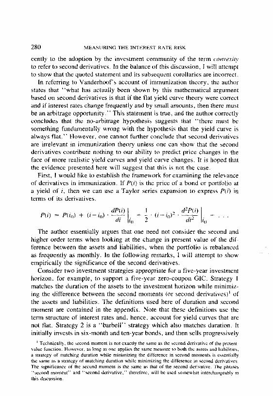
An investor with a 10-year time horizon is considering two portfolio strategies:

!. Buy the 10-year zero (exact cash match to the horizon). 2. Manage an immunized portfolio which is duration matched to the horizon.

The immunized portfolio consists primarily o f the 30-year bond. There will be a small position in money market instruments to achieve an exact duration match. The portfolio is rebalanced periodically to match its duration to the zero coupon.

We are going to look at the relative performance over a six-month period. Our assumptions are:

1. Yields on the two bonds always move by the same amount. 2. The standard deviation of yields is 120 basis points per year.

The two bonds start out with the same duration. Without taking convexity into account, an investor might look at the respective yields and decide that the zero-coupon bond is the better investment.

Now let us actually compare the components o f return: yield, duration, and convexity.

Yield - y~ = . I0 , Y2 = .099.

The zero has a 10 basis point yield advantage.


Duration- 1 0 P i Di - - 9.53

Pi 0Yl 1 BP,

De - " - 9.53. P2 0Y2

This term will be the same for both bonds regardless of interest rate move.

Convexi ty- 1 02PI Ci - - 95.2

Pl O)'~

1 02p2 - - 160.8.

C2 P 2 0y~

Under continuous rebalancing, the impact of convexity on annualized 1

return is ~ Ci o2.

Based on our assumed ¢r = .012, the difference in convexity gains for these two bonds translates into 47 basis points per year.

Under our assumptions, the 30-year bond has a 37 basis point per year advantage over the zero (47 from convexity minus 10 from yield).

The Short Term Rate. Earlier we mentioned that the immunized portfolio would contain some money market investments. This was in order to adjust duration to match the 10-year zero. Our analysis, however, did not consider the effect of short-term investments on the yield.

The reason for this is that the percentage of short-term assets in the portfolio is so small that it has virtually no impact. Since initial durations are equal, there is no short-term position at the outset. As yields change, the durations will differ slightly requiring some rebalancing with short-term assets. Over the six-month period, however, it will not be enough to make a significant difference.

Continuous Versus Periodic Rebaluncing. Converting convexity into a nonstochastic term really depends on continuous rebalancing. By letting our rebalancing interval, ~ t , become small, we experience the effect of averaging (law of large numbers) over any given period.

Continuous rebalancing, however, is unrealistic because of the high transaction costs it generates. Less frequent rebalancing, on the other hand, will introduce more variance into our returns. In practice, a balance should be reached between reducing risk (variance) and trading costs.

If there are N rebalancings over a period, then the cumulative convexity effect has a ×2 distribution with N degrees of freedom. 3

For example, with monthly rebalancing over a 6-month period, the total

3 This assumes that convexity is fairly constant over the time period. For most bonds this is a reasonable assumption, For options on bonds, however, convexity changes too rapidly to justify the assumption.

DISCUSSION 273

convexity gains of the 30-year bond relative to the zero has a X 2 distribution with 6 degrees of freedom. It has a mean of 47 basis points in annualized return and a standard deviation of 27 points.

Correction of Mispricing. We have begun with the assumption that the zero's yield was 10 basis points higher than the 30-year bond. Since this yield spread does not adequately compensate for the zero's lower convexity, the bond actually has a 37-point per year advantage.

This assumes that the 10 basis point yield spread remains fixed over time. Suppose, though, that the mispricing suddenly corrected itself, i.e., that the spread increased from 10 points to 47 points. Over the course of that correction, the bond would outperform the zero by 350 basis points.

This correction is the heart of arbitrage: not the small gains that accrue slowly when mispricing persists, but the rapid reversal of the mispricing which telescopes all the future gains into one point in time.

Yield Volatility. Our mispricing conclusion has depended on the assumption that the standard deviation of changes in yield is 110 basis points per year. Unlike price and yield, this is unobservable in the market and can only be estimated.

If we had estimated a lower volatility, the effect of convexity (which is proportional to variance) would have been diminished. In our example, it would take a volatility of 50 basis points per year before the mispricing would go away.

The role of the volatility assumption here is very much akin to its role in option pricing, An option, like bond convexity, is more valuable the more volatile the underlying asset, a

Basis Risk. The weak link in our whole analysis is the assumption that the respective bond yields move in parallel. This is especially true at the shorter end of the yield curve where shape changes are most pronounced.

At the longer end, the shape is more fiat and is much less subject to change. Because of this, the yield changes in longer bonds show a high level of correlation. (It is partly for this reason that our example uses long bonds.) Even so, yields on long bonds will not move in exact parallel leaving us with some basis risk.

Basis risk can be analyzed by estimating correlation and regression coefficients of one bond's yield relative to the other. This allows us to estimate the basis risk (e.g., determine its standard deviation).

Under basis risk we can no longer say that one asset will always outperform another. What we can say, however, is that it is likely for one asset

a This similarity is no coincidence. An option is a decaying asset in the sense that its value will decline if the underlying asset price or yield remains unchanged. One could thus think of an option as having a negative yield. What compensates the investor for the negative yield is the option's extreme convexity.


to outperform another. The degree of yield correlation will determine just how likely that is.

APPLICATIONS TO ASSET-LIABILITY MANAGEMENT

Another Way of Viewing Convexity

The duration of a coupon bond will change as its yield changes. More specifically, duration decreases with rising yield and increases with falling yield. Because of this, a 1 percent drop in yield will change the bond price by a greater absolute amount than a 1 percent rise. But this is exactly the effect of convexity.

We now have another way of looking at convexity-- the extent to which duration changes with a change in yield. Armed with this approach, we can next look at some typical general account assets.

CALLABLE BONDS AND MORTGAGE PASS-THROUGHS

Callable bonds and pass-throughs have low and sometimes even negative convexity. An intuitive way of seeing this is to realize that higher interest rates extend the maturities (and therefore durations) while lower rates shorten maturities. This is in the opposite direction of convexity, where durations move inversely to yields.

In the case of mortgage pass-throughs, the borrowers prepay the loans more rapidly in a low interest rate environment but avoid prepayment when rates are high. In the case of corporate bonds, the likelihood of call is inversely related to the yield level.

LIFE INSURANCE COMPANY LIABILITIES

What we saw on the asset side was that options in the hands of the borrower remove convexity from the investor's portfolio. On the liability side, it is the options of the contract holders that increase liability convexity.

These options crop up in almost every conceivable investment and interest- sensitive product. For guaranteed investment contracts (GICs) there are de- posit options and book-value withdrawal features. Universal life, whole life, and SPDAs have book-value features which are equivalent to put options. The more sophisticated the contract holders are the more valuable the option.

PORTFOLIO MANAGEMENT

Life insurance companies are in tight competition to offer high yields on investment products. This, in turn, places increasing pressure to invest in high yielding assets. Unfortunately, the tendency is to back high convexity

DISCtJSSIOrq 275

liabilities with low convexity assets in search for this higher yield, while ignoring convexity in the pricing.

By ignoring asset and liability options and the convexity gap that results, phantom profit margins are created. These margins can only materialize if yields remain stable. Under volatile interest rates, the convexity deficit will erase any profit margin. The disintermediation experience of the early 1980s is testimony to the power of volatile interest rates.

ELIAS S. W. SHIU:

Professor Milgrom is to be thanked for reminding us that there is no free lunch. In view of the many interest-sensitive products in the marketplace, this is certainly a timely paper. The following are some remarks on the paper.

C. D. Rich [6] is perhaps the first person to point out that the second derivative profit in Redington's model does not occur in practice. P. P. Boyle also mentions this fact in his paper [1], which won the 1978 Halmstad prize.

I am puzzled by the statement that " i f A and L have equal present values and equal vulnerabilities when evaluated at market interest rates, then the no-arbitrage hypothesis implies that PVj j (A; I )=PVj j (L; I ) . "

Denote the surplus

PV(A;I) - PV(L;I)

by S(1). It is assumed that

Sj(I) = 0, j = 1,2 . . . . . k.

By the no-arbitrage hypothesis, the function S cannot have a maximum or a minimum at I. This implies that the Hessian matrix (second derivative) of S at I, (So(I)), is neither positive definite nor negative definite. Without further assumption, it cannot be proved that

Sjj(I) = 0, j = 1,2 . . . . . k,

which, however, is the conclusion in the statement quoted previously. I would like to present a generalization of the model discussed in the last

part of the paper. Given a force-of-interest function 5(.), the present value of a stream of cash flows {C~} is

fo ~ C, e x p ( - g(s) ds),

which we shall denote by S(g). (If we consider each C, as At - L,, then

276 M E A S U R I N G T H E I N T E R E S T R A T E R I S K

S(~) = PV(A;~) - PV(L;~) . )

Suppose that the force-of-interest function changes from ~(-) to ~ ( - ) . Then what is

S ( ~ j ) - S ( ~ ) ?

fo Define ct = Ctexp( - ~(s) ds),

~(t) = ~l(t) - ~(t)

and

Then

and

DmCUSSION 277

Interchanging the order of summation and integration yields the equation

c, ( (t - w) f " (w) dw) = ( ~ c, (t -- w)) f " (w) dw. I : :0 ) 1='),~'

Now, suppose that the cash flows {C,} are such that either

c,(t - w) ~ 0 for all positive w (2) l - w

or

c,(t - w) ~ 0 for all positive w; (3) I~) ) '

then, by the mean-value theorem for integrals, there exists a positive number such that

f o ( ~ c,(, -- w ) ) f " ( w ) d w = f"(~) fo ( ~ G(t - w))dw.

Reversing the order of integration and summation, we have

fo ( ~ ct(t - w)) dw = ~ c, ( (t - w) dw) t - - ~t' t - ' O

= . ~ c, (t2/2). t>'O

(4)

Thus, subject to (2) or (3),

S(a l) S(8) -E(O) Z tG + ~ f" (~) Z t2 - - ~ C t .

If, in addition to (2) or (3), we also assume that the first moment of the present values of the cash flows is zero, i.e.

tc, = 0, (5) t~O

then

S(8,) - S(8) = ~ f (4) ~ t2 c,. (6) t_=-O

Observe that, because of equation 4, the term

f 2 Ct t--O

(7)

is nonnegative if (2) holds and nonpositive if (3) holds. Also note that, since


f " ( s ) = fis)t(~(s)) 2 - e'(s)] for all s,

the sign o f f " ( ~ ) is the same as that of

( ~ ( 0 ) 2 - ~ ' ( O -

Equation 6 implies that, subject to (5) and (2) or (3), the term 7 or its absolute value can be used as a measure of the interest rate risk of the cash flows. For the case where there is only one positive cash outflow, an expression similar to (7) has been derived by Fong and Vasicek [3], and it is described as a measure of risk for an immunized portfolio. For a simple derivation of the Fong-Vasicek result, see [5]. Note that, if

Z t2 Ct "~- 0, (8) t>O

then, for each interest rate shock e,

S(8 + ~) = S(8). (9)

However , if (5), (8), and (2) or (3) hold, then, for each t > 0, C, = 0, and thus, we have (9).

Equation (6) suggests a strategy, conservative with respect to interest rate fluctuations, for structuring the cash flows of a line o f business: Solve for {C,} by minimizing expression 7 subject to (2), (5), and any other necessary constraints or by maximizing (7) subject to (3), (5), and any other necessary constraints. However , since the point ~ depends on the cash flows {C,} (and the interest rate shock e), minimizing

] Z t2c, I

does not necessarily imply that

I f " (~) ~ t2 c, [ t~O

is minimized even for a fixed function ~. For more details on this model, see [7] and [8]. Let me conclude this discussion with some quotations on duration match-

ing, Fisher and Weil [2] claim that the reduction in risk provided by a duration matching strategy is " s o dramatic that . . . a properly chosen portfolio of long-term bonds is essentially r iskless." However, a recent paper by Ingersoll 14] says:

Academic research in this area has multiplied many fold. Most of it has been concerned with correcting or replacing Macaulay's measure to fine tune a portfolio manager's ability to immunize, There have not, however, been any published tests of these new models. Indeed even the Fisher and Weil test has not been independently confirmed,

DtSCUSSION 279

In this paper, we review the Fisher-Weil findings and report substantially different findings when a similar test is performed on the quoted bond prices in the CRSP Government Bond File . . . . Since Durand's yield curves and those similarly constructed would tend to smooth out this effect, it could account for the discrepancy between our results and those of Fisher and Weil. But if this explanation is correct, then there is little hope for the practical application of Macaulay's duration in immunization . . . . In repeating the Fisher-Weil immunization tests on quoted bond prices, we found that immunizing through duration matching did nowhere near as well as they report. On an absolute scale we found the remaining risk to be larger by a factor of 10. On a relative scale we found that duration matching could not consistently beat the more naive scheme of maturity matching.

REFERENCES

1. BOYLE, P. P. "Immunization Under Stochastic Models of the Term Structure," J1A, CV (1978), 177-86.

2. FmHER, L., AND WELL, R. L. "Coping with the Risk of Interest-Rate Fluctuations: Returns to Bondholders from Naive and Optimal Strategies," Journal of Business, XLIV (1971), 408--31.

3. FONG, H. G., AND VASXCEK, O. "A Risk Minimizing Strategy for Portfolio Im- munization," Journal of Finance, XXXIX (1984), 1541-46.

4. INGERSOLL, J. E., JR. "Is Immunization Feasible? Evidence from the CRSP Data," Innovations in Bond Pororolio Management: Duration Analysis and Immunization, edited by G. G. Kaufman, G. O. Bierwag, and A. Toevs, Greenwich, Connecticut: JAI Press inc., 1983, 163-82.

5. PROKOPETZ, M. U., AND SHIU, E. S. W. Discussion of. l .D. Stiefel's "'The Guar- anteed Investment Contract (GIC)," TSA, XXXVI (1984), 569--73.

6. RICH, C. D. Discussion of F. M. Redington's "Review of the Principles of Life Office Valuation," JIA, LXXVIII (1952), 319-21.

7. SHIU, E. S. W. "Immunization---The Matching of Assets and Liabilities," Proceed- ings of the Symposia in Statistics and Festschrift in Honour of V. M. Joshi, edited by I. B. MacNeill and G. J. Umphrey, Dordrecht, Holland: D. Reidel Publishing. To be published.

8. ~ . "A Generalization of Redington's Theory of Immunization," ARCH, 1986.

ROBERT P. CLANCY:

Professor Milgrom has produced a timely paper on a subject of great interest to actuaries. His derivation of the term structure of interest rates from economic fundamentals is a fine one and should considerably improve actuaries ' understanding of spot and forward rates. However, I must take issue with his statement that " the no-arbitrage hypothesis implies that there is no place in immunizat ion theory for measures based on second derivatives of the present-value func t ion . " This statement rejects not only the referenced work by Vanderhoof but also the work of such widely respected researchers

as Fong and Vasicek, Diller, and Til ley (see [2], 13], [4], [6], and [7]). The importance of second derivatives in immunizat ion theory has led even re-

2 8 0 M E A S U R I N G THE I N T E R E S T R A T E RISK

cently to the adoption by the investment community of the term convexity to refer to second derivatives. In the balance of this discussion, I will attempt to show that the quoted statement and its subsequent corollaries are incorrect.

In referring to Vanderhoof's account of immunization theory, the author states that "what has actually been shown by this mathematical argument based on second derivatives is that if the fiat yield curve theory were correct and if interest rates change frequently and by small amounts, then there must be an arbitrage opportunity." This statement is true, and the author correctly concludes that the no-arbitrage hypothesis suggests that " there must be something fundamentally wrong with the hypothesis that the yield curve is always f la t . " However, one cannot further conclude that second derivatives are irrelevant in immunization theory unless one can show that the second derivatives contribute nothing to our ability to predict price changes in the face of more realistic yield curves and yield curve changes. It is hoped that the evidence presented here will suggest that this is not the case.

First, I would like to establish the framework for examining the relevance of derivatives in immunization. If P(i) is the price of a bond or portfolio at a yield of i, then we can use a Taylor series expansion to express P(i) in terms of its derivatives.

I 1 d2p(i) I __dP(i) + - • ( i - i0) 2 • - - q- . . . P(i) P(io) + ( i - i ° ) " di io 2 di 2 i o

The author essentially argues that one need not consider the second and higher order terms when looking at the change in present value of the difference between the assets and liabilities, when the portfolio is rebalanced as frequently as monthly. In the following remarks, I will attempt to show empirically the significance of the second derivatives.

Consider two investment strategies appropriate for a five-year investment horizon, for example, to support a five-year zero-coupon GIC. Strategy 1 matches the duration of the assets to the investment horizon while minimizing the difference between the second moments (or second derivatives) j of the assets and liabilities. The definitions used here of duration and second moment are contained in the appendix. Note that these definitions use the term structure of interest rates and, hence, account for yield curves that are not fiat. Strategy 2 is a "barbe l l " strategy which also matches duration. It initially invests in six-month and ten-year bonds, and then sells progressively

t Technically, the second moment is not exactly the same as the second derivative of the present- value function. However, as long as one applies the same measure to both the assets and liabilities, a strategy of matching duration while minimizing the difference in second moments is essentially the same as a strategy of matching duration while minimizing the difference in second derivatives. The significance of the second moment is the same as that of the second derivative. The phrases - second momen t" and "second der ivat ive ," therefore, will be used somewhat interchangeably in this discussion.

DISCUSSION 281

the long bonds, placing the bond sales proceeds in new six-month bonds in order to match the target duration.

Strategy 2, therefore, calls for the assets to be considerably more dispersed than the liabilities, and the difference between the second moments of the assets and liabilities is greater than in Strategy 1. Suppose further that we happen to be in a flat yield-curve environment at 10 percent. Table 1 summarizes the results for two parallel yield-curve shifts.

The results in table 1 are hardly startling, and they conform to classical immunization theory. Strategy 2 outperforms Strategy 1 when parallel yield- curve shifts occur. This result was predictable from the relative magnitudes of the second moments of the two strategies. However, as Professor Milgrom points out, these results are somewhat irrelevant since "yield curves are not flat and do not maintain the rigid shape prescribed by our assumptions as they vary over t ime." It is precisely for these reasons that considerations of second moments (or derivatives) are important.

Consider now a nonparallel shift in the yield curve which represents a tilt in the yield curve. For example, suppose that we make our initial investments in the same flat 10 percent yield-curve environment as before. Suppose further that yields on six-month bonds suddenly drop to 7 percent while yields on ten-year bonds remain at 10 percent, and yields on all intermediate length bonds are obtained by linear interpolation. If the yield curve holds this positively sloped shape for the remainder of the time horizon, then the estimated performance results under each of the strategies would be as shown in table 2. Two alternative yield-curve shifts with the same slope in which the ten-year bond rate moves 300 basis points are also analyzed.

Comparing table 2 with table 1, one can see that the results are extremely sensitive to the slope of the assumed yield curve but not too sensitive to the level of the yield curve. In fact, moving the positively sloped yield curve up or down 300 basis points (the last two scenarios in table 2) has just about the same effect on each strategy as parallel shifts of the same magnitude, as shown in table 1. One can see also that a shift to a positively sloped yield curve results in Strategy 2 drastically underperforming Strategy 1. This order of performance is the exact opposite of that obtained from table 1 for a

T A B L E 1

REALIZED YIELDS OVER 5-YEAR HORIZON

Yield-Cur',e Shift Strategy I Strategy 2

I. NO Shift 10.00% 10.00% 2. up 300 basis points 10.04 10.13 3. down 300 basis ix~ints 10.04 10.14


TABLE 2

REALIZED YIELD OVER 5-YEAR HORIZON

Yield-Cure Shift

6-Month Rate 10-Year Rate

7~ ~o~ 4 7

I0 13

Strategy I

9.65% 9.72 9.66

Strategy 2

8.87% 9.02 9.02

parallel yield-curve shift. This result was also predictable using the following nontechnical reasoning. If the second moment for a duration-matching strategy indicates the sensitivity o f that strategy to a parallel yield-curve shift, then could it not also indicate the sensitivity of that strategy to a nonparallel shift? In fact, Fong and Vasicek define the second moment , M 2, as an index of sensitivity to a change in shape of the yield curve. This concept is central to the "s ta te of the ar t" immunization systems currently on the market. These systems try to find the duration-matching portfolio which is least sensitive to parallel yield-curve shifts.

I concede that 1 would get slightly different results if I assumed more gradual yield-curve shifts and continuous rebalancing. Even if the results did differ dramatically, such sensitivity of results would be of great importance to a prospective portfolio manager who wishes to ignore second moments. In this event, the portfolio manager would realize that one can obtain the theoretically predicted result only by continuous rebalancing rather than rebalancing at less frequent intervals, such as the one-month interval suggested by the author. O f course, the portfolio manager might then have significant transaction costs.

In any event, I believe the results with continuous rebalancing and gradual yield-curve shifts would not be different enough to alter the conclusions put forth above. Fong and Vasicek confirm the reasonableness of my suspicion with the following insightful observation 13]:

It is not difficult to see why a "barbell" portfolio composed of very short and very long bonds should be more risky than a "'bullet" portfolio consisting of low coupon issues with maturities close to the horizon date. Assume that both portfolios have durations equal to the horizon length, so that both portfolios are immune to parallel rate changes. When interest rates change in an arbitrary non-parallel way, however, the effect on the two portfolios is very different.

Suppose, for instance, that short rates and long rates increase. The end-of-horizon values of both portfolios would fall below the target, since both portfolios would experience a capital loss in addition to lower reinvestment rates. The decline however, would be substantially higher for the barbell portfolio than for the bullet portfolio, for two reasons. First, the barbell portfolio experiences lower reinvestment rates for a

DISCUSSION 283

longer time interval than the bullet portfolio, so its opportunity cost is much greater. Second, the portion of the barbell portfolio still outstanding at the horizon date is much longer than that of the bullet portfolio, which means that the same rate increase will result in a much steeper capital loss for the former. The low M 2 bullet portfolio has less exposure to whatever the change in the interest rate structure may be than the high M 2 barbell portfolio.

In short, one can perfect ly immunize a set of l iabil i t ies against all kinds of y ie ld-curve shifts only by invest ing in a portfol io which perfect ly matches the l iabi l i ty f lows. In this event , first, second, and all h igher order der ivat ives of the present value of the assets would match those of the l iabil i t ies. Match- ing first der ivat ives alone is not suff icient to assure immuniza t ion in the real wor ld o f nonparal le l y ie ld-curve changes. Matching first and second deriv- at ives is safer than matching only durat ion. To refute the s ignif icance of the second der ivat ive ( commonly referred to as convexi ty) is to refute the work o f leading researchers and pract i t ioners in the inves tment communi ty . I con- c lude that convexi ty measures are re levant in immuniza t ion theory.

REFERENCES

1. BIERWAG, G.O. "Immunization, Duration, and the Term Structure of Interest Rates,'" Journal of Financial and Quantitative Analysis, December 1977.

2. DmLER, STANLEY. "'Parametric Analysis of Fixed Income Securities," Goldman Sachs & Co., June 1984.

3. FONG, n. GIFFORD, AND VASICEK, OLDRICH. "The Tradeoff Between Return and Risk in Inmnunized Portfolios," Financial Analysts Journal, September/October 1983.

4. ~ "A Risk Minimizing Strategy for Portfolio Immunization," Journal of Fi- nance, XXXIX, No. 5, December 1984, 1541-.-46,

5. KLOTZ, RICttARD G. "Convexity of Fixed Income Securities," Salomon Brothers Inc., October 1985.

6. TILLEY, JAMES, BUFF, JOSEPH, NORIS, PETER, AND LORD, GRAHAM. Discussion of the paper by Robert P. Clancy "Options on Bonds and Applications to Product Pricing," TSA, XXXVII (1985), 134.-45.

7. VANDER~OOF, IRWIN. "Interest Rate Assumptions and the Relationship Between Asset and Liability Structure," Study Note 8-201-79, Chicago, 111.: Society of Ac- tuaries.

APPENDIX

DEFINITIONS

C F t = cash f low at t ime t f rom bond or portfol io Y, = spot rate for d iscount ing payments at t ime t, i .e . , the term

structure of interest rates D i = durat ion of bond or portfol io (first moment )


D 2 = second moment of bond or portfolio

t.CF,.(l + y,)- ' l

D 1 =

CFt.( I + y , ) - ' I

t2"CFt'( 1 + Yt)- ' t

D 2 =

CF/(1 +Yt) - ' t

B E N J A M I N W. W U R Z B U R G E R : *

B A C K G R O U N D A N D S U M M A R Y

Professor Milgrom claims that setting V i = 0 (the first derivative of the net present value) will ensure that the change in V over any short period will be second order in time. t Were this claim valid, it would have important im- pl icat ions- implicat ions that Professor Milgrom does note: (1) A strategy of matching asset and liability first derivatives, in conjunction with very frequent rebalancing, would suffice to guarantee that V be unaffected by rate movements. (2) A GIC intermediary who practices frequent rebalancing need not he concerned with second derivatives. This implication would invalidate the standard actuarial wisdom that it is very important to calculate second derivatives.

Professor Milgrom's claim is, however, incorrect. In the first half of my comments, I shall explain that setting Vi = 0 without also setting Vii = 0 will ensure that the changes in V will be first order in time. Second derivatives are therefore crucially important. It turns out that Professor Milgrom is off by one derivative--recent work has demonstrated that it is legitimate to neglect third derivatives.

In the second half of my comments, I discuss at length the actual deter- minants of the evolution of V, devoting special attention to the case where the assets are more dispersed than the liabilities. I derive a formula for the evolution of V in terms of the underlying parameters of the yield curve dynamics and the asset and liability second moments.

IT IS I N V A L I D TO N E G L E C T T H E S E C O N D D E R I V A T I V E

I begin with some notation. Let PA denote the present discounted value of the assets, PL the liability present value, and V = PA - P L the net present

* Dr. Wurzburger, not a member of the Society, is an economist in the Financial Research and Risk Analysis division at the John Hancock.

i More precisely, the changes in V attributable to interest rate movements would be proportional to (&t) 2.

DISCUSSION 285

value. Let Vi = P A i - P L i denote the first derivative of V with respect to the interest rate index. ~- Let AW represent the change in V attributable to interest rate movements. This superscript notation emphasizes that V can change for many reasons above and beyond movements in i; for example, the passage of time will affect V even if rates do not change. I now discuss why the standard specification of the interest rate dynamics implies that AV i is first order in time even though V i= O.

The standard assumption has rates following a Brownian motion diffusion process, otherwise known as a Wiener process. (For those more comfortable with the binomial formulation, I shall shortly rederive the major result under that framework.) In other words, if the interest rate is now i o, the interest rate t periods hence will be normally distributed with mean io and variance o'21, where o" is the "volati l i ty." Formally, interest rates follow the stochastic differential equation

di = o'dw ( 1 )

where dw is the increment to a Wiener process w. 3 Let us now expand d W (the differential of the change in V attributable to rate movements) as a Taylor series in i.

dV i = Vidi + Vii(di)2/2 (2)

Equation (2) neglects the (di) 3 and the higher-order terms, which is ac- ceptable. By hypothesis

Vi = 0 and (di) 2 = 0 -2 (dw) 2 = o-2dt, so

dV i= Viio-2dt/2. (3)

Even though V i = 0, the change in V attributable to rate movements is first order in time (on the order of dt), in contradiction to Professor Milgrom's

z For simplicity one can think of a model with a single interest rate i, so yield curve shifts are perforce parallel. More generally, one can incorporate systematic nonparallel shifts by regarding i as an index of interest rates, so Vi represents the sensitivity to that index.

3 w follows a Wiener process if w ( q ) - w ( t o ) has a normal distribution with mean zero and variance t~ - t o . It can be shown that this implies (dw) 2= dt. The right-hand-side (r.h.s.) of (1) does not include any deterministic component, only a pure stochastic term, so the expected value of the r.h.s, is zero. Because of the absence of a deterministic component, the specification is strictly speaking an equilibrium-type model; in practice, economists explicit ly forecast and the yield curve implici t ly forecasts both the direction and the magnitude of change, so Eidi) , the expected change, may be non-zero. The condition E(d i )=O is often described as the zero-drift condition.

It is also olten standard to modify ( 1 ) to make the increments proportional to i so that di = cridw. Under this specification i will be lognormally distributed. (The classic Black-Scholes [1] work assumes stock prices are Iognormal, and Clancy [2] also assumes interest rates are Iognormal.) Neither of these complicat ions-- introduct ion of a disequilibrium non-zero E(dil or making the r.h.s. proportional t o / - - w o u l d affect the thrust of this section.


claim that the condition Vi= 0 will ensure that changes be second order in time.

A similar result can be demonstrated in the binomial framework of interest rate movements. Recall that in the binomial framework (e.g. Clancy [2]), i moves in any small time period to either i+~r(A) In or i -¢ r ( • t ) t/2. (This is a binomial with zero drift and constant or, the finite analogue of equation 1.) Thus, (~ i )2= ~r2~t. A Taylor series expansion implies

A V i = V i i i + Vii(hi)2~2 + higher-order terms, (4)

so V i = 0 implies ~ V i = Vi i t r2~t /2 , i.e. first order in time. Why is AV i first order in time even though the first term in the Taylor

series vanishes? Because changes in interest rates are on the order of the square root of time, so that squared changes are first order in time. With this insight, I can now present a corrected version of Milgrom's footnote (page 253): If the relevant time period between rebalancing is one month, 1/12 of a year, then the change in interest rates will be on the order of (1/12) 1/2, and the squared value is 1/12, a fraction which is not negligible. Klotz {5], Tilley [7], Wurzburger [8], and others are therefore correct when they advocate paying close attention to the second derivative Vii.

What about third and higher order derivatives? In the Brownian motion example (equation 2) I asserted that the third and higher order derivatives could be neglected. I asserted this result rather than proving it since my primary purpose was to emphasize the importance of the second derivative. It is a relatively straightforward exercise (the quickest way would involve applying Ito's Lemma (see Malliaris and Brock, [6]) to demonstrate that for Brownian motion, equation 3 is exact and third derivatives are irrelevant. Garman [4[ has recently extended this result and shown that for all reasonable continuous-time processes, third and higher order derivatives are irrelevant " in the small ."

I conclude that Milgrom is off by one order of derivative in his claim that the second derivative Vii is unimportant--it is the third derivative Vii i that is unimportant.

THE EVOLUTION OF THE NET PRESENT VALUE OVER TIME

The first part of my remarks has concentrated on the change in V attributable to changes in i, the index of interest rates? A more complete analysis would recognize that V also depends explicitly upon time, i.e. V= V(i,t).

(The passage of time raises the present discounted value of both the asset

4 Recall (footnote 2) that interpreting i as an index allows the analysis to incorporate systematic nonparallel shifts.

DISCUSSION 287

and liability cash flows.) Let Vt denote the partial derivative of V with respect to t. Clearly, our earlier equations must be augmented by a V t term. Hence,

dV = Vflt + Vidi + Vii(r2dt/2. (5)

For those familiar with lto's Lemma, equation 5 is the partial differential equation for the system V= V(i , t ) ,d i=trdw. Since I agree with Professor Milgrom about the importance of setting V i = 0, I shall restrict the analysis to such cases. Hence,

dV/dt = Vt + Viio'2/2. (6)

Let us consider the standard case where the present values of assets and liabilities are equal (V=0) , and to make the analysis interesting, I will assume that the assets are more dispersed than the liabilities. (It is nowadays characteristic of GIC intermediaries that their assets are more dispersed.) By assumption both V and Vi are zero, and we want to discuss the evolution of V, namely dV/dt. For simplicity we are restricting ourselves to equilibrium- type analysis (see footnote 3). I now discuss the two terms in (6).

The V t term: In equilibrium, the yield curve should be concave. (The yield curve is typically concave, i.e., the curve lies above the straight line joining any of its two points.) Accordingly, excess asset dispersion tends to make Vt negative--intuitively, the concave yield structure implies that the dispersed assets earn, on average, a lower yield than the concentrated liabilities. 5

The Vii t e r m : While PAii and PLii are both positive, Vii = P A i l - P L i i will be positive provided the assets are more dispersed. This positivity is a classical result from immunization theory and also follows from the analysis in the appendix of this discussion. While excess asset dispersion is adverse from the Vt standpoint, it is favorable from the Vii cr 2 standpoint. 6

In the appendix, I apply several first order approximations to equation 6 and derive a formula describing how excess asset dispersion contributes to dV/dt. Let M 2 (A) denote the second moment of the (discounted) asset stream and M2(L) the second moment of the liabilities. Let b denote the slope of the (spot-rate) yield curve, c the concavity term, and h the coefficient cap- turing the systematic nonparallel yield shift. (If h = 0, we are in the world

s The systematic tendency for nonparallel shifts, with short rates more volatile than the long. partially offsets this concavity. Because of this systematic nonparallel s-~fift, the condition Vi = 0 implies that the dispersed assets will have a higher duration than the liabilities. This higher duration raises the yield, provided the yield curve is upward sloping. For a derivation, please see the appendix.

An asset 's second derivative is often described as its convexity (e.g. Klotz I5]). Convexity refers to the shape of the price-yield curve. Concavity, in our V, discussion, refers to the shape of the yield-maturity curve. It is noteworthy that convexity of the price-yield curve offsets the concavity of the yield-maturity curve.


of parallel shifts.) The parameters b, c, and h have been defined so that they are all positive. I have derived the following equation:

dV/dt= [M2(A)-M2(L)] × (0-2/2+ 2 b h - 3c). (7)

As discussed, volatility and the systematic nonparallel shifts favor asset dispersion, while yield curve concavity argues contrarily. An intermediary, therefore, ought to estimate the equilibrium value of 0-2/2 + 2 h b - 3c, hence- forth denoted as Q.

In his paper, Professor Milgrom (page 254) observes that one would like a model to be consistent with the no-arbitrage hypothesis. Superficially, it would appear that if we estimate Q to be, say, positive, 7 our model then contradicts the no-arbitrage hypothesis: a zero V is earning a positive V t. I note three reasons why an estimate of a positive Q would not guarantee, in fact, that excess asset dispersion generates riskless profits: 1. The analysis is equilibrium-based and, therefore, might not apply to a

particular disequilibrium situation. Under reasonable assumptions about yield-curve disequilibrium dynamics, however, Q would have the same value in disequilibirum as in equilibrium, even though the individual components may differ.

2. It is difficult to estimate the relevant parameters. For example, cr is not stationary. Even if one has estimated that Q is positive, and excess asset dispersion is a desideratum, it might turn out that Q is actually negative.

3. Our formula assumes a simple index, namely any single maturity determines all the other rates. In particular, the model implies that short-term and long-term rates always move in the same direction. In practice, it is of course possible for short-term rates to decline while long-term rates increase. As Fong and Vasicek [3] have observed, such a steepening of the yield curve would be very adverse for an intermediary that displays excess asset dispersion. Multi-index models of the term structure would generate more complicated formulas, and the second derivative term would involve third and higher-order moments.

In conclusion, second derivatives and second moments are crucial for determining the evolution of the value of a portfolio.

REFERENCES

I. BLAre:K, F., AND SCHOLES, M. "The Pricing of Options and Corporate Liabilities," Jourmd of Political Economy 81 (1973), 637-59.

2. CLANCY, R.P. "Options on Bonds and Applications to Product Pricing," TSA, XXXVII (1985), 97-151.

7 My own preliminary econometric work has not yet provided an unambiguous answer about the sign of Q.

DISCUSSION 289

3. FONG, H.G., AND VASlCEK, O. "A Risk Minimizing Strategy tbr Portfolio Immu- nization," Journal of Finance, 39 (1984). 1541----46.

4. GARMAN, M.B."Towards a Semigroup Pricing Theory," Jourmd of Finance, 61 (1985), 847.-.61.

5. KLOTZ, R.G. "'Convexity of Fixed Income Securities," Salomon Brothers, October 1985.

6. MALLIAR~S, A.G., AND BROCK, W.A. Stochastic Methods in Economics and Fi- nance, Amsterdam: North Holland, 1982.

7. TILLEY, J. "Risk Control Techniques for Life Insurance Companies," Morgan Stan- ley, June 1985.

8. WURZBURC~ER, B.W. Discussion of paper by Robert P. Clancy "'Options on Bonds and Applications to Product Pricing," TSA, XXXVII (1985), 131-34.

APPENDIX

DERIVATION OF THE FORMULA dV/d! = M 2 (o'2/2 + 2 b h - 3c)

Let r9N) denote the spot zero-coupon spot rate as a function of maturity, i.e. the present discounted value (P .D.V.) o f 1 dollar N periods hence is e -r~N)N. (I use the notation r instead of i to emphasize that r is a function of N.) We assume the following term structure behavior for our equilibrium analysis:

r = a + b N - c N 2, (1)

and dr = o-( 1 - hN)dw. (2)

All the parameters, a, b, c, and h are assumed to be positive. The c term implies that the yield-curve is concave, and the b term is positive so that the yield curve is upward sloping. The h term reflects the fact that short rates are more volatile than long rates; a rate increase will be systematically associated with a flattening of the yield curve. The equation neglects potential nonsystematic changes.

Let A(N) and L(N) denote the cash-flow streams. Thus, the net present value is

V = ~ (A - L ) e rN (3)

From a Taylor series expansion ( I to 's Lemma),

KV = Vtdt + Vrdr + Vrr(dr)2/2. (4)

2 9 0 MEASURING THE INTEREST RATE RlSK

now Vt = VN (the passage of time reduces the maturity by an equal increment.) Thus, dV = - VNdt + Vrdr + Vrr(dr)2/2, and (5)

d - r ( N ) N (3) and (1) imply - V N = ~ - ( a - L)e -rN

dN

= ~ ( A - L ) e - r N ( a + 2 b N - 3 c N 2) = a M ° + 2 b M j - 3 c M 2, (6)

where MJ is the jth moment of the net P.D.V. M ° is thus the net P.D.V. Provided M ° = 0 , M ~ is the difference in duration times the asset (or liability) present value. M 2 is the difference in the second moments.

Combining (3) and (2), Vrdr = ~ ( - N) (A - L)e- rN O'( 1 - - h N ) d w

= _ ~rdw(M I - hM2) . (7)

The condition V r d r = O (first-order insensitivity, analagous to Milgrom's condition Vi = 0) implies M l = h M 2. (8)

Thus, if the assets are more dispersed than the liabilities (a positive M2), Vrdr = 0 implies that the assets ought to display a greater duration than the liabilities. Substituting M l = h M 2, M ° = 0, into (6)

V, = - VN = ( 2 b h - 3c)M 2. (9)

Similarly, Vrr(dr)2/2 = ~ N2(A - L)e rNo'2 (1 - hN)2(dw)2/2 = cr2dt(M 2 - 2 h M 3 + h2M4)/2. (10)

Under reasonable conditions (the first order approximauon that h is small so that h M 3 and h2M 4 are small relative to M2), (10) implies

Vrr(dr)2/2 = ff2M2 dr~2. (11)

Combining (11), (9), and (4),

dV/d t = M2(cr2/2 + 2 b h - 3c). (12)

ALBERT K. CHRISTIANS:

Professor Milgrom is to be commended for a presentation that reaches thought-provoking conclusions directly from simple and fundamental prem- ises. His recommendation that we are our limited knowledge of interest rate

DISCUSSION 291

fluctuations to avert large losses rather than to seek small profits is com- pelling.

Among the provacative elements of his theory is Professor Milgrom's extremely inclusive definition of arbitrage. The dictionary defines arbitrage as a set of simultaneous transactions that produce a gain immediately. Pro- fessor Milgrom expands this to include transactions that will produce a certain profit after an interval of time if interest rates follow the arbitrageur's hypothesis. Such intertemporal arbitrage opportunities would not arise in an idealized system following the author's implicit assumptions, and he shows that the assumptions of the Macaulay-Redington immunization theory are inconsistent with his.

A crucial feature of Professor Milgrom's assumptions seems to be that the mechanism by which interest rates and yield curves are determined should be able to operate in a world possessing complete information about its operation. My guess is that ignorance is an important part of the process of yield curve determination and that developing a theory of immunization to apply in a world of complete information is an exercise in contradiction.

The author's assumption that arbitrage opportunities do not arise must be considered a first order approximation. Its approximate accuracy may be sustained, however, by arbitrageurs who profit by exploiting second order exceptions to its rule. Any financial institution or intermediary with a need to immunize its portfolio should fall within Professor Milgrom's definition of an arbitrageur and could not exist if the author's assumptions were perfectly accurate.

Thus, the paper makes clear the difficulties of deriving a practical approach to immunization when assuming efficient, rational, and perfectly informed markets. This leads me to hypothesize that the need for immunization strategies arises because of the differences between ideal and real markets. This also seems to demonstrate a limit to the applicability of solutions derived from simple models.

DOUGLAS A. ECKLEY:

Professor Milgrom covers a variety of aspects of interest rate analysis, and his commentary is thought-provoking in every case. My purposes in discussing his paper are to provide further commentary in two places, to provide numeric illustrations of some concepts, to disagree with one conclusion drawn by Professor Milgrom, and to espouse the applicability of the random walk theory to interest rates.

In section II of his paper, the author discusses interest rates in terms of period-by-period rates. In section III, he turns to the more customary characterization of interest rates, which is in terms of yields to maturity. This


characterization is often referred to as the yield curve. To understand these concepts, one must realize that a set of period-by-period rates does not determine a set of yield rates, or vice versa. To derive one from the other a specific cash-flow stream is required (except in the trivial case where all of the period-by-period interest rates are equal). This is illustrated in the followb~g tables using two specific cash-flow streams: 8 percent bonds with semiannual coupons maturing in year t, and Treasury Zeros maturing in year t.

To generate a yield rate in the "8% Bonds" column, the cash-flow stream of an 8 percent bond is discounted using the year-by-year interest rates. The yield rate shown is the yield rate an investor would earn if he purchased the bond for an amount equal to the present value. This shows that the term yield curve has no definition without reference to a specific cash-flow stream. In fact, different cash-flow streams can produce materially different yield curves given the same year-by-year interest rates.

Year-by Year Yew Ra~s

T /{~ 8~ Bonds I 0 .1000 0. I 00000 2 0.0950 0.097679 3 0.0900 0.095462 4 0.0850 0.093339 5 0.0800 0.091299 6 0.0750 0.089335 7 0.0700 0.087435 8 0.0650 0.085594 9 0.0600 0.083802

10 0.0550 0.082052 11 0.0500 0.080340 12 0.0500 0.078875 13 0.0500 0.077604 14 0.0500 0.076-490 15 0.0500 0.075502

Year by-Year Yew Rates

T 1t13 8% Bonds 1 0 .1000 0. I00000 2 0.1050 0.102315 3 0.1100 0.104516 4 0.1150 0.106610 5 0.1200 0.108598 6 0.1250 0.110484 7 0.1250 0.111828 8 0.1250 0.112833 9 0.1250 0.113611

10 0.1250 0.114229 I1 0.1250 0.114731 12 0.1250 0.115145 13 0.1250 0.115491 14 0.1250 0.115784 15 0.1250 0.116035

Yield Rates

Yield Rates

~ros 0.100000 0.097497 0.094992 0.092486 0.089977 0.087466 0,084954 0.082439 0.079923 0.077404 0.074884 0.072788 0.071017 0~069502 0.068191

~ros

0.100000 0.102497 0.104992 0,107486 0.109977 0.112467 0.114249 0.115587 o.116629 0.117463 0.118147 0~118716 0.119198 0.119612 0,119970

DISCtJSSION 293

Professor Milgrom refutes the theory that interest rates fluctuate randomly about a normal level. Readers should not confuse this theory, which is invalid, with that of the random walk, which I believe to be applicable to interest rates. The random walk theory states that changes in. not the levels of, stock or commodity prices are random. Interest rates do measure the price of a commodity (borrowed funds).

Few random walk theorists maintain that their model is applicable beyond the short term. The theory allows for Ion-term trends reflecting intrinsic value changes. The short-term perspective makes the long-term trend im- material. Factors affecting the long-term intrinsic value of borrowed funds probably include inflation, a large and persistent borrower such as the United States government, and actions of the Federal Reserve Board.

A major premise of the random walk theory is that the market is efficient. An insider would bias price changes until the information in his possession became widely distributed. In an efficient market, the disagreement of informed people provides one element of randomness. But price changes would be random even if everyone always agreed as to intrinsic value. This is because the supply and demand for borrowed funds reflect expectations. These expectations are changed in light of new events and new information. The new events and new information fall on either side of expectations in random fashion. In a world of uncertainty, new events cause random changes in commodity prices and interest rates. This is not to say that one who had better insight than his peers cannot profit.

Professor Milgrom is a strong believer in the no-arbitrage hypothesis. This hypothesis, like the random walk theory, is premised upon an efficient market. He reasons from this hypothesis that taking second derivatives of interest rate functions is inappropriate. I agree and would go further by saying that taking first derivatives of interest rate functions is inappropriate. Taking a derivative implies that the interest rate can be expressed as a function of a finite number of parameters. This, in turn, implies more knowledge of the shape of the yield curve than one can ever obtain. Any function of a finite number of parameters has possible values numbering the first order of infinity. On the other hand, the number of possible yield curves is on the second order of infinity. Any representation of a yield curves as a differ- entiable function is, at best, an approximation. Professor Milgrom and I agree that the approximation can be close enough to reality to be useful.

Professor Milgrom goes on to argue that if two different cash-flow streams have equal present values and equal first derivatives, then the no-arbitrage hypothesis implies that they also have equal second derivatives. The type of analysis rejected by this argument is illustrated in the following table.

The flaw in this table is that the yield curve is assumed to be linear with unchanging slope. This allows the construction of a cash-flow portfolio whose


YEAR:

YIELD CURVE AT PURCHASE:

NEW YIELD CURVE SHAPE:

CASH FLOWS:

3 6 9

0.0700 x

- ! , o o o . o o

0.0750 x + . 0 0 5 0

- 1 , 0 0 0 . 0 0

YIELD TO VALDE OF ARIcII'/'RAGE YEAR 3 PORTFOLIO GA/N

- 754.4457 - 754.6762 - 754.8809 - 755.0602 - 755.2143 - 755.3438 - 755.4489 - 7 5 5 . 5 3 0 1 - 7 5 5 . 5 8 7 6

- 755.6219 - 755.6332 - 755.6220 - 755.5885 - 755.5332 - 755.4563 - 755.3581 - 755.2390 - 755.0993 - 754.9393 - 754.7594 - 754.5597

0.0600 0.0610 0.0620 0.0630 0.0640 0.O650 0.0660 0.0670 0 . 0 6 8 0

0 . 0 6 9 0

0.0700 0.0710 0.0720 O. 0730 O. 0740 0.0750 0.0760 0.0770 0.0780 0.0790 0.0800

1.1875 0.9570 0.7523 0.5730 0.4189 0.2894 0.1843 0.1031 0.0456 0.0113 0.0000 0.0112 0.0447 0.1000 0.1770 0.2751 0.3942 0.5339 0.6939 0.8739 1.0735

0.0800 x + .0100 1,416.55

value can only increase on changes in interest rates. The illustrated portfolio has cash outflows of $1,000 in years 3 and 6 and an inflow of $1,416.547 in year 9. If the year 3 yield rate is 7 percent, this portfolio, whose value is a liability, could be assumed on receipt of $755.63. The non-zero second derivative of the value of this portfolio is illustrated in the table. Before trying to construct this portfolio, the speculator must realize that this table expresses interest rates as a function of a finite number of parameters. The following table illustrates the flaw.

This table illustrates that a minute change in the shape of the yield curve produces a loss for the dream portfolio. The new yield-curve shape was not allowed for in the simple model used to produce the portfolio. A more complicated model could be developed to allow for this shape also. In fact, Professor Milgrom does just this in section IV of his paper. However, any model involving a finite number of parameters cannot allow for all possible yield-curve shapes.

I must disagree with Professor Milgrom's conclusion in section III that "immunizing effectively against the losses suffered from small changes in I over all short periods also solves the larger problem of immunizing against the large movements in I that may take place over longer periods." His

D I S C U S S I O N 295

YEA R:

YIELD CURVE AT PURCHASE:

NEW YIELD CURVE SHAPE:

CASH FLOWS:

0.0700 x

- 1 , 0 0 0 . 0 0

0.0750 x + . 0 0 5 1

- 1 , 0 0 0 . 0 0

YIELD TO VALUE OF ARBITRAGE YEAR 3 PORTFOUO GAIN

- 755.3647 - 755.5757 - 7 5 5 . 7 7 1 0 - 7 5 5 . 9 4 0 9 - 7 5 6 . 0 8 5 9 - 756.2063 - 7 5 6 . 3 0 2 4 - 7 5 6 . 3 0 2 4 - 756.4234 - 756.4489 --756.4516 - 756.4319 - 7 5 6 . 3 9 0 0 - 7 5 6 . 3 2 6 3 - 756,2411 - 7 5 6 . 1 3 4 8

- 756.0076 - 755.8600 - 755.6921 - 755.5043 - 7 5 5 . 2 9 7 0

0.0600 0.0610 0.062O 0.063O 0.0640 0.065O 0.0660 0.0670 0.0680 0.0690 0.0700 0.0710 0.0720 0.0730 0,0740 0.0750 0.0760 0.0770 0.0780 0.0790 0.0800

0.2785 0.0575

- 0.1378 - 0 . 3 0 7 7 - 0 . 4 5 2 7 - 0 . 5 7 3 1 - 0.6692 - 0 . 7 4 1 4 - 0 . 7 9 0 1 - 0 . 8 1 5 7 - 0.8184 - 0 . 7 9 8 7 - 0 . 7 5 6 8 - 0 . 6 9 3 1 - 0.6079 - 0 . 5 0 1 6 - 0 . 3 7 4 4 - 0 . 2 2 6 7 - 0.0589

0.1289 0.3363

0.0800 x + .0102 1,416.55

reasoning is that equality of first derivatives implies equality of second derivatives, else a portfolio could be constructed which resulted only in gains. Since this reasoning makes use of derivatives, it implies that interest rates are a function of a finite number of parameters. I have stated that this cannot be valid, but even if it is valid, it contradicts earlier statements by Professor Milgrom. For example, the interest function must either be consistent with the no-arbitrage hypothesis or inconsistent with it. If the former, then it is untested as stated by Professor Milgrom in section III. If the latter, then the second derivatives are not necessarily equal. Finally, Professor Milgrom stated that there is no place in immunization theory for second derivatives.

Although I disagree with one of Professor Milgrom's conclusions, I found his paper to be most scholarly.

J A M E S M. R O B I N S O N :

I would like to congratulate Professor Milgrom on his thought-provoking analysis of the measurement of the interest rate risk. I offer a brief discussion of the traditional immunization model presented in section III of the paper, especially with regard to the existence of arbitrage opportunities. I hope that


my comments and any subsequent remarks that Professor Milgrom might add will help clarify the points already presented.

Again, consider a yield curve g(t) = ~ + 2x(t), where ~(t) is a shape component and 8 establishes the overall level of interest rates. Now, let v(t)

= exp { - f ~ 8(s) ds}, the discount factor generated by such a yield curve. If it is assumed that only g varies in the short run while A(t) remains

fixed, then arbitrage opportunities will always exist. To see this, consider the following construction,

Given L = (LI, L2 . . . . . L,,), structure A = (AI, A 2 . . . . . A,z) in the following manner. For some arbitrary k such that 1 < k < n, define

{ L s. i 4: k - l , k, k + l

Ai = L i - 1, i = k L i + v ( k ) / 2 v ( k - 1 ) , i = k - 1 Ls + v ( k ) / 2 v ( k + 1), i = k + 1.

In other words, use exact matching to support all but $1 of the liability stream. For the remaining $1, purchase assets of equal present value maturing one period prior and one period after the duration at which this $1 is due to be paid. It is easily shown that the asset and liability structures have equal present values and durations. Furthermore, the second derivative of the assets with regard to changes in 8 is greater than that for the liabilities.

P V ( A - L , g ) = { v ( k ) / 2 v ( k -

+ {v(k) /2v(k +

- - 0 - d P V ( A - L , g)/dg = {v(k)/2v(k -

+ {v(k)/2v(k +

= 0 a e P V ( A - L , g)/d82 = { v ( k ) / 2 v ( k -

+

l ) } v ( k - l ) - {1}v(k) l ) } v ( k + 1)

1)}(k- l ) v ( k - 1) - {l}kv(k) 1)} (k+ I)v(k+ I)

l ) } ~ k - l~2~,~k - l ) - {1}kz,,~k)

{v (k ) /2v (k+ 1)}(k+ 1)2v(k+ 1) v(k) {k z - 2k + 1 - 2k 2 + k 2 + 2k + 1}/2

= v(k) > 0

Therefore, the present value of the assets will be greater than or equal to the present value of the liabilities for 8 sufficiently close to the current value of ~. Since interest rates are almost certain to vary, an arbitrage opportunity exists. That is, the preceding technique would seem to be a fool-proof recipe for creating surplus.

The no-arbitrage hypothesis argues that such a technique may not survive in an efficient market. Consequently, there must be something wrong with this development. Professor Milgrom contends in section Ill that flat yield curves (i.e., Z~(t) = 0) produce arbitrage potential. This is certainly supported in the previous example. However, Professor Milgrom goes on in a

DISCUSSION 2 9 7

footnote to state that a linear form for •(t) may be constructed which is consistent with the no-arbitrage hypothesis. I find this difficult to reconcile with the previous findings, which apply to any reasonable form for ~( t ) . Perhaps the author could help explain this apparent inconsistency in his response to the discussions.

What is wrong with the previous analysis? The only significant assumption required is the constancy of ~( t ) as 8 varies. At this point, I can only conclude that in a market in which arbitrage opportunities are nonexistent, A(t) must vary as well as 8. As Professor Milgrom points out, unless we have some knowledge about feasible variations in A(t) and b, we cannot hope to develop a practical measure of the interest rate risk. The author's two-factor yield structure and the associated first order sensitivity indexes are certainly more palatable than the overly simplistic counterparts in the traditional Macaulay-Redington model. With these points in mind, I tend to agree with Professor Milgrom's contention that the various immunization factors presented in the paper are not reliable measures of the total exposure to the risk of varying future interest rates but are more appropriately used as sensitivity indexes for a variety of speculated types of interest variations.

(AUTHOR'S REVIEW OF DISCUSSION)

PAUL R. MILGROM:

I would like to thank all the discussants for their comments, which serve to expand, elucidate, and in one case correct the points made in my paper. It was especially gratifying to find so much agreement--or at least so little disagreement--with the economic approach to present value theory that I described, ~ even though that theory diverges importantly from the traditional actuarial approach.

The discussion by Messrs. Buff and Lord brings out practically some of the issues I explored abstractly. The discussants focus their comments on the kinds of errors that are frequently made in evaluating the status and vulnerability of financial security plans. Their concrete listing of the dangers of using book values in place of market values for evaluating C-3 risk are well worth studying. But this listing of dangers is not their only contribution. They also highlight the problems that arise when the cash flows to be immunized may themselves be sensitive to interest rates. That is a problem of enormous practical importance not only for managing portfolios and measuring the interest rate risk, but also for the valuation of liabilities. For valuations, the difficulty is that the cost of a portfolio that matches the cash- flow pattern of the liability will generally depend on the interest sensitivity of the cash flows.

This approach was first developed more than half a century ago by the American economist Irving Fisher, It has since become the standard approach used in textb~vaks on microeconomics.

2 9 8 M E A S U R I N G THE I N T E R E S T R A T E RISK

It is important to recognize that the difficulty in valuing and immunizing interest-sensitive cash flows is not one of principle. The Vj indexes can (in principle) be computed exactly as specified in my paper regardless of the interest-sensitivity of the cash flows. The real difficulty is that there is little precise information about how the cash flows of even such major classes of financial security plans as life insurance and pensions actually respond to shifting interest rates. Failure to account for interest sensitivities introduces biases into the index calculations. For example, if annuity holders delay making withdrawals in order to take advantage of interest guarantees when market interest rates are below the contractually guaranteed rates, then falling interest rates increase liabilities more than otherwise; the index understates the true sensitivity of the present value of annuity payments to changing interest rates.

General statements about the biases introduced by interest-sensitive cash flows are hard to make because so little is known about how people actually respond to changing interest rates. Research shedding light on this matter would be of great value.

Four of the discussants, Messrs. Levin, Shiu, Clancy, and Wurzburger, have spotted an error in my treatment of second derivatives of the present- value function. (They also provide a formal mathematical treatment, using the Ito stochastic calculus, of some of the same issues I treated.) I had mistakenly argued on the last page of section III that if "A and L have equal present values and equal vulnerabilities" then the second derivatives of the present-value functions PV(A; I) and PV(L; 1") with respect to the interest rate indexes must also be equal. I relied on this statement to reach the incorrect conclusion that frequent portfolio rebalancing is not critical for approximate immunization.

The correct argument, rendered here in plain English, goes as follows. If A and L have equal present values and vulnerabilities (evaluated at market interest rates), then the random variations in their returns 2 over the next short interval of time will be equal--that is how the vulnerability indexes were constructed. Then, if the mean returns over the next short time interval for A and L are not equal, the stream with the higher mean will always have the higher return over the next short interval of time so that there is an arbitrage opportunity. Therefore, assuming the no-arbitrage hypothesis, equalizing vulnerability measures assures that the two streams have precisely equal returns over the next short interval.3 This argument confirms that, as

2 Around, say. the mean return. 3 Those facile with the Ito calculus can check the corresponding formal steps of this argument as

follows. Equal vulnerabilities and present values imply that the diffusion coefficients of the values of A and L are equal, Then. the no-arbitrage hypothesis implies that the drift coefficients are also equal. For, otherwise, the investment portfolio corresponding to A - L would have zero net cost, non-zero drift, and zero diffusion coefficient; that is. it would be an arbitrage portfolio.

DISCUSSION 299

I had claimed, only first derivative measures of vulnerability are necessary for immunization if poroColios can be rebalanced suffficiently frequently. And, importantly, for nonimmunized portfolios, these same vulnerability measures correctly reflect the risk the portfolio faces in the near term due to shifting interest rates.

The foregoing argument is not inconsistent with the argument advanced by several discussants that convexity (second derivative based) measures have a role to play in immunization theory. To maintain effective immunization over time without frequent (and expensive) rebalancing, one needs to arrange the portfolio so that the vulnerabilities of A and L remain nearly equal as time passes and interest rates change. One does this by equating the derivatives of the vulnerability measures with respect to time and the interest rate indexes. The latter involves second derivatives of the present- value function. Mr. Levin makes precisely this point when he says that convexity can be viewed as the "extent to which duration changes with a change in yie ld ."

The upshot of the foregoing analysis is that using both first and second derivative based measures for immunization reduces the need for frequent portfolio rebalancing. For portfolios that are not fully immunized because immunization is but one of several objectives and for which vulnerability measures are needed, the indexes derived from first derivatives of the present-value function are probably adequate.

Two of the discussions, those of Mr. Shiu and of Messrs. Buff and Lord, assess the success of the Macaulay-Redington index in practice. While Messrs. Buff and Lord are optimistic about the value of the Macaulay-Redington index (arguing that immunization using that index is, as a practical matter, effective), Mr. Shiu cites a study by my colleague, Jon Ingersoll, who finds in a study of managed portfolios that the immunization using the Macaulay- Redington duration measure is ineffectual for eliminating the interest rate risk.

Given the strength of the theoretical arguments against the Macaulay- Redington duration index, Ingersoll's empirical findings are as expected. Certainly, no well-trained actuary would expect a single mortality " l eve l " index to capture the subtle shifts in age/sex-specific mortality changes that occur over time and are important to insurance pricing; that is why detailed mortality studies are continually conducted by the life insurance industry. Imagine how much less satisfactory a single mortality index would be if the highest mortality rates occurred sometimes at the young ages and sometimes at the old, and "overa l l " rates were sometimes rising and sometimes falling! That is precisely the case for interest rates: short-term rates are sometimes higher and sometimes lower than long-term rates, and the whole twisting structure rises and falls quite suddenly. Just as mortality rates are key for


all life insurance pricing, interest rates are key to bond pricing and liability valuation. Any sensible person can see that a single index based on the overall " l e v e l " of interest rates cannot represent the shifts of this kind adequately for liability valuation.

As I have emphasized in my paper, measures of risk are based on theories of interest rate movements, that is, theories that impose some restrictions on the term structure of interest rates and how it may change over time. The Macaulay-Redington duration measure is based on the theory that interest rates at all durations move up and down together equally and in unison. That model errs substantially in its description of actual interest rate movements. Shifts in the shape of the yield curve can and sometimes do have large effects on the solvency of financial security plans, even when the Macaulay- Redington duration measure says the risk is zero. Empirical studies normally operate by averaging the performance of the Macaulay-Redington index over those times when it works well and those when it fails. For a decision maker, the most telling point to emerge from the data is that the Macaulay-Redington index is unreliable, and it is most unreliable precisely when it is most needed, which is when the cash-flow streams of assets and liabilities are far from being matched. The favorable empirical studies, which average the good performance of Macaulay-Redington-immunized portfolios when the streams are well matched with the bad performance of Macaulay-Redington-immunized portfolios which are not well matched, are cold comfort to a manager who needs a reliable guide to measuring risks.

Mr. Christian's main criticism of my article is founded on his view that the no-arbitrage hypothesis is just a first order approximation and that any worthy financial institution ought to be looking for arbitrage opportunities to exploit. He then hints that such an institution ought to be suspicious of a risk measure based on the no-arbitrage hypothesis, such as any of the measures I have mentioned. However, Mr. Christian's argument does not justify the hinted conclusion.

In saying that the no-arbitrage hypothesis is a "first approximation," one might sensibly mean that financial institutions, from time to time, can identify arbitrage opportunities but not on so large a scale as to limit the institution's ability to finance other investments. Then, surprisingly, the economic theory of market valuation I have described applies exactly; that is, the economic value of a cash-flow stream is its present value computed using the interest rates implicit in the bond prices of the arbitrage-free portion of the market. Indeed, nothing in the argument given in my paper is affected by the presence of the limited arbitrage opportunities described previously: It is still true that an asset is worth no more or less than the cost of duplicating its cash flows by trading in liquid bonds. If the asset is cheaper than the corresponding bonds, one would still want to sell the bonds and make the

DISCUSSION 301

investment. If the investment were dearer, it would still be better to buy the bonds.

This is not to say that the economic valuation theory described in my paper is exactly right for the world we actually live in, with its illiquidities, tax consequences of trading, and interest-sensitive cash flows. My point is much more limited in that the no-arbitrage hypothesis need not hold exactly in order for the theory and its associated risk measures to be useful. Indeed, as we have seen, the theory is unchanged if one weakens the no-arbitrage hypothesis to allow limited arbitrage opportunities to arise from time to time.

Mr. Eckley criticizes the use of immunization theories and measures in principle, since they depend on parametric assumptions about the yield curve- - assumptions which are only approximations, and possibly poor ones. I have already emphasized that these theories and measures do depend on assumptions about the shape of the yield curve. There are both theoretical and empirical reasons to believe that the yield curve does have some structure, although that does not guarantee that we will be able to isolate the structure in a useful way. Mr. Eckley 's cautions are well-warranted.

Nevertheless, the only proper reason to eschew the use of all parametric yield curves is that one can do as well without them. Indeed, as Mr. Eckley argues, there may be some situations in which matching is perfectly appropriate and immunization indexes are dispensable. I suspect, however, that actuaries more often find matching strategies to be inadequate. How should an actuary advise a client who rejects matching because immunization is but one of his several objectives? Should he eschew all vulnerability measures because they are imperfect? How should managers who would like to approach perfect immunization proceed when the cash flows to be immunized are interest sensitive'? Matching in such a case may be impossible, and then immunization using measured vulnerabilities is presently the only alternative.

I have emphasized the word presently, because it is certainly conceivable that actuaries sharing Mr. Eckley 's views could develop " theory-f ree" measures of vulnerability that expand the domain of matching ideas. For example, one might say that the M-vulnerability index (M for matching) is defined as the maximum, over all nonnegative, year-by-year interest rates, of the excess in present value of the liability stream over the asset stream. For perfectly matched streams, the measure is zero. For other streams, it represents the worst-case loss from shifting interest rates. It is my guess that worst-case indexes will never be as useful as the kinds of indexes described in my paper: The worst case described is quite extreme, and attempts to account for more realistic variations in interest rates amount to reintroducing an interest rate theory through the back door. However, the matter is still far from resolved.


Mr. Robinson's discussion proves the claim in my paper that the Macau- lay-Redington flat curve theory of interest rates contradicts the no-arbitrage condition. He does this by showing how one can create a spread which, with certainty, performs better than a given original portfolio if the yield curve is always fiat. He then further argues, mistakenly, that the same spread rules out all theories of the term structure of interest rates in which the continuously compounded rate of interest rate at date t has the rigid form:

~(t) = ~ + A(t),

where ~ is subject to stochastic changes. However, when A(t) is not flat, the original and spread portfolios have different yields, and the inferior convexity of the original portfolio may be compensated by its higher yield. When A(t) is chosen exactly to compensate for differences in convexity, there is no arbitrage opportunity here, contrary to Mr. Robinson's assertion.

I have tried to keep my review of the discussants' remarks reasonably brief and free of complicated mathematical arguments. I hope that readers fluent in the stochastic calculus will forgive me for the consequent lack of rigor, and that the discussants who used these techniques will forgive me for my necessarily incomplete review of their comments. My choices have been guided by a desire to communicate the principal, relevant, economic ideas to the widest possible actuarial audience. I will be most gratified if actuaries who have not mastered economics, finance, and the Ito stochastic calculus find my paper and review of the discussions to be illuminating or, at least, stimulating.

Date post:	24-Jan-2022
Category:	Documents
Upload:	others
View:	2 times
Download:	0 times

TRANSACTIONS OF SOCIETY OF ACTUARIES 1985 VOL. 37 ...

Documents