26
Transdimensional Markov Chain Monte Carlo Methods Jesse Kolb, Vedran Lekić (Univ. of MD) Supervisor: Kris Innanen
Transdimensional
Markov Chain Monte Carlo
Methods
Jesse Kolb, Vedran Lekić (Univ. of MD)
Supervisor: Kris Innanen
Motivation for Different Inversion
Technique
• Inversion techniques typically provide a single best-fit
model while the fit of other models may be only slightly
worse.
• Inversion algorithms often get stuck in local minima.
• Non-uniqueness is often uncharacterized.
• Dimensionality (e.g. number of layers) may be unknown
prior to inversion.
• Uncertainty analysis is desired on individual features
within a result.
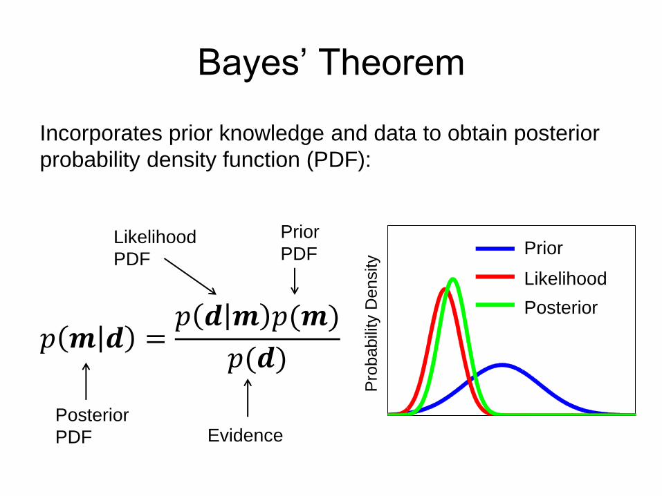
Bayes’ Theorem
Incorporates prior knowledge and data to obtain posterior
probability density function (PDF):
𝑝 𝒎 𝒅 =𝑝 𝒅 𝒎 𝑝(𝒎)
𝑝(𝒅)
Posterior
Likelihood
Prior
Evidence
Prior
Likelihood
Posterior
Pro
babili
ty D
ensity
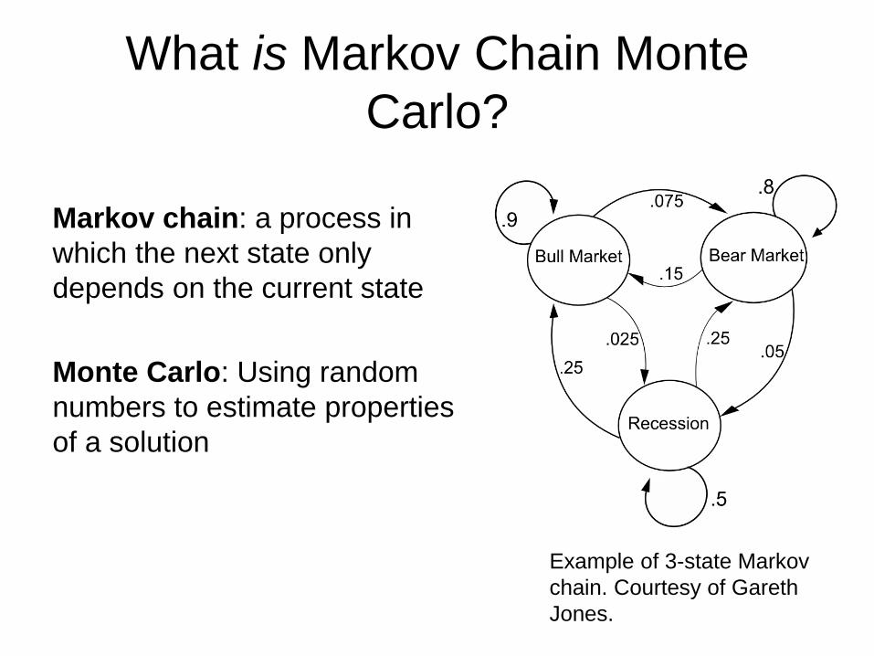
What is Markov Chain Monte
Carlo?
Markov chain: a process in
which the next state only
depends on the current state
Monte Carlo: Using random
numbers to estimate properties
of a solution
Example of 3-state Markov
chain. Courtesy of Gareth
Jones.
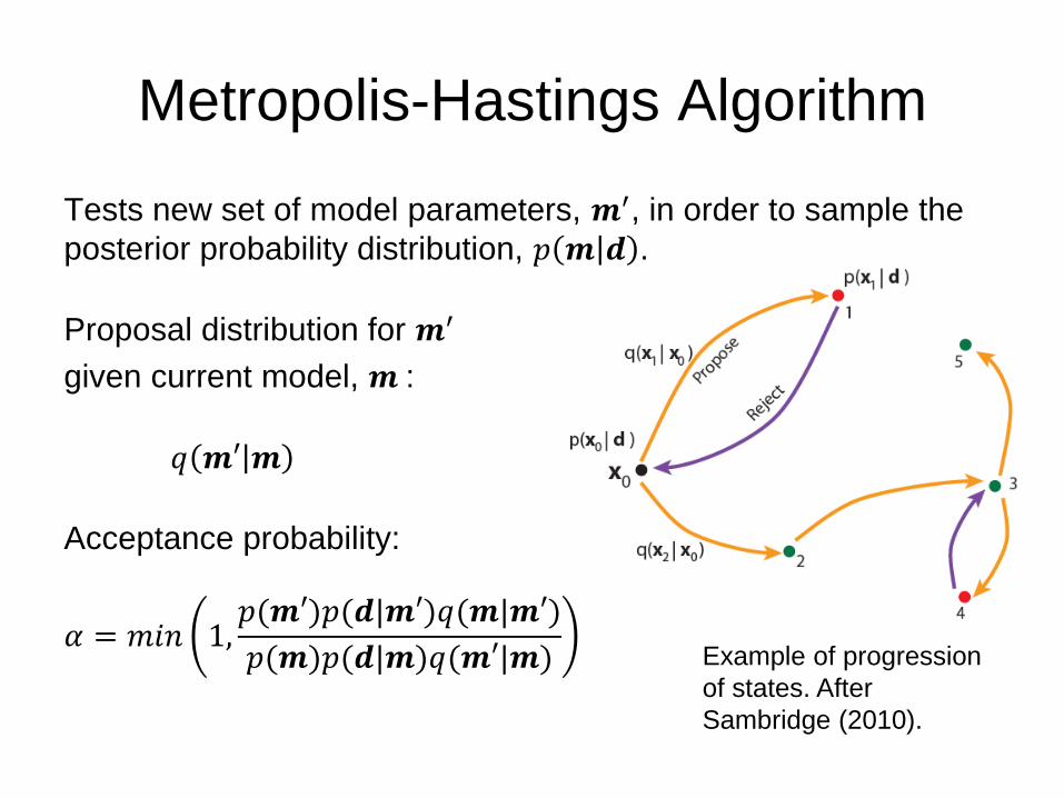
Metropolis-Hastings Algorithm
Tests new set of model parameters, 𝒎′, in order to sample the
posterior probability distribution, 𝑝 𝒎 𝒅 .
Proposal distribution for 𝒎′
given current model, 𝒎 :
𝑞 𝒎′ 𝒎
Acceptance probability:
𝛼 = 𝑚𝑖𝑛 1,𝑝(𝒎′)𝑝(𝒅|𝒎′)𝑞(𝒎|𝒎′)
𝑝(𝒎)𝑝(𝒅|𝒎)𝑞(𝒎′|𝒎)
Example of progression
of states. After
Sambridge (2010).
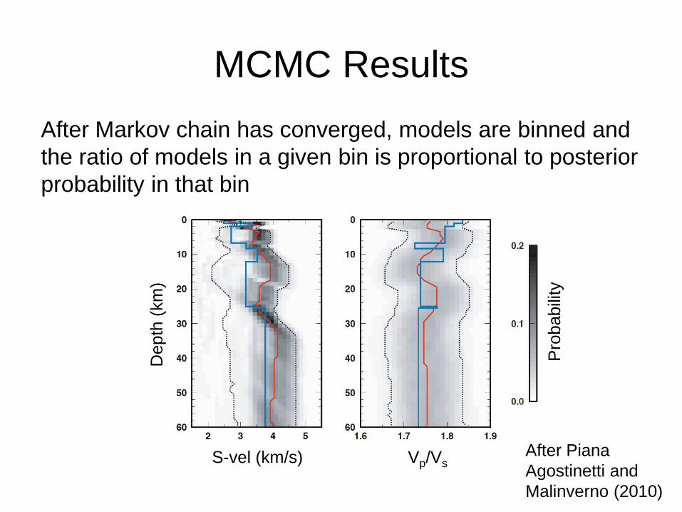
MCMC Results
After Markov chain has converged, models are binned and
the ratio of models in a given bin is proportional to posterior
probability in that bin
S-vel (km/s) Vp/Vs
Depth
(km
)
Pro
babili
ty
After Piana
Agostinetti and
Malinverno (2010)
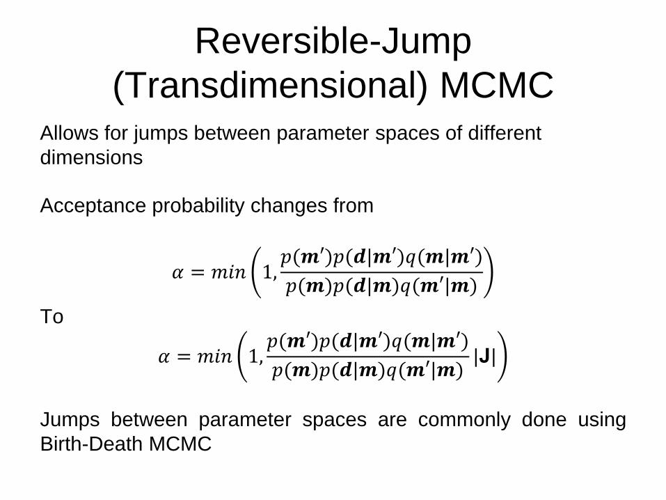
Reversible-Jump
(Transdimensional) MCMC Allows for jumps between parameter spaces of different
dimensions
Acceptance probability changes from
𝛼 = 𝑚𝑖𝑛 1,𝑝(𝒎′)𝑝(𝒅|𝒎′)𝑞(𝒎|𝒎′)
𝑝(𝒎)𝑝(𝒅|𝒎)𝑞(𝒎′|𝒎)
To
𝛼 = 𝑚𝑖𝑛 1,𝑝(𝒎′)𝑝(𝒅|𝒎′)𝑞(𝒎|𝒎′)
𝑝(𝒎)𝑝(𝒅|𝒎)𝑞(𝒎′|𝒎)|J|
Jumps between parameter spaces are commonly done using
Birth-Death MCMC
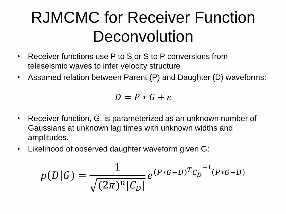
RJMCMC for Receiver Function
Deconvolution • Receiver functions use P to S or S to P conversions from
teleseismic waves to infer velocity structure
• Assumed relation between Parent (P) and Daughter (D) waveforms:
𝐷 = 𝑃 ∗ 𝐺 + 𝜀
• Receiver function, G, is parameterized as an unknown number of
Gaussians at unknown lag times with unknown widths and
amplitudes.
• Likelihood of observed daughter waveform given G:
𝑝 𝐷 𝐺 =1
(2𝜋)𝑛|𝐶𝐷|𝑒 𝑃∗𝐺−𝐷
𝑇𝐶𝐷−1𝑃∗𝐺−𝐷
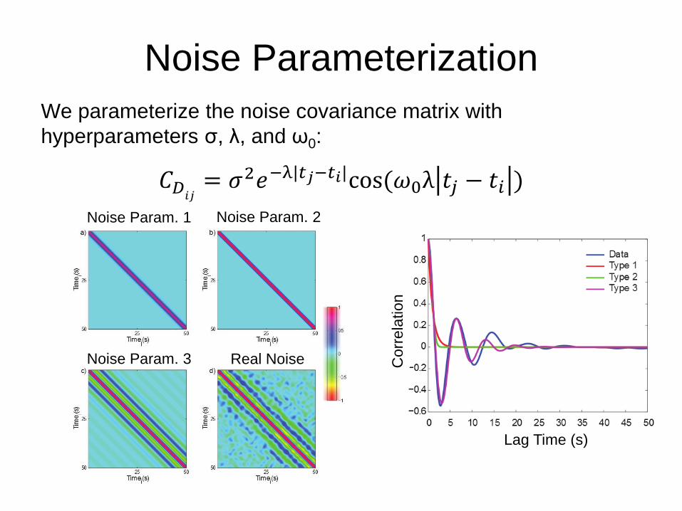
Noise Parameterization
We parameterize the noise covariance matrix with
hyperparameters σ, λ, and ω0:
𝐶𝐷𝑖𝑗= 𝜎2𝑒−λ|𝑡𝑗−𝑡𝑖|cos (𝜔0λ 𝑡𝑗 − 𝑡𝑖 )
Noise Param. 1 Noise Param. 2
Noise Param. 3 Real Noise
Lag Time (s)
Corr
ela
tion
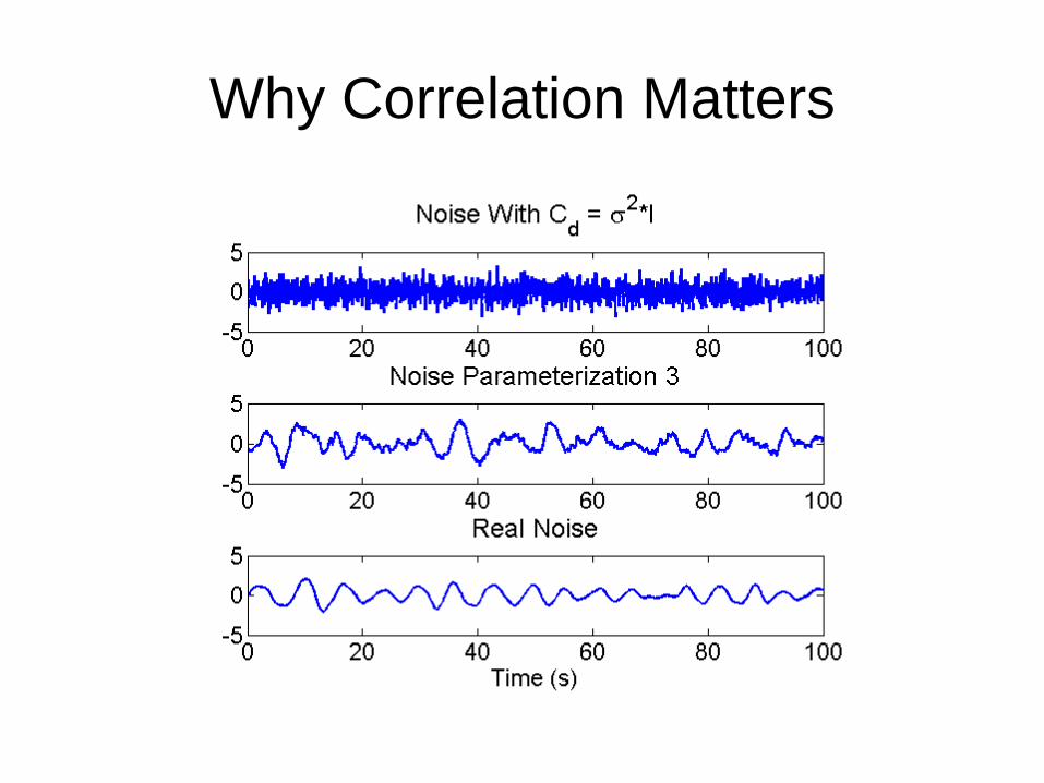
Why Correlation Matters
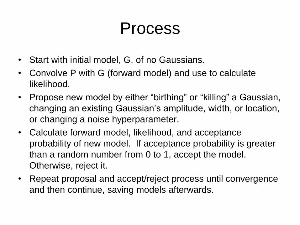
Process
• Start with initial model, G, of no Gaussians.
• Convolve P with G (forward model) and use to calculate
likelihood.
• Propose new model by either “birthing” or “killing” a Gaussian,
changing an existing Gaussian’s amplitude, width, or location,
or changing a noise hyperparameter.
• Calculate forward model, likelihood, and acceptance
probability of new model. If acceptance probability is greater
than a random number from 0 to 1, accept the model.
Otherwise, reject it.
• Repeat proposal and accept/reject process until convergence
and then continue, saving models afterwards.
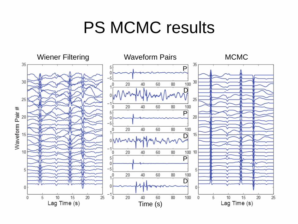
PS MCMC results
Wiener Filtering Waveform Pairs MCMC
Time (s)
P
P
P
D
D
D
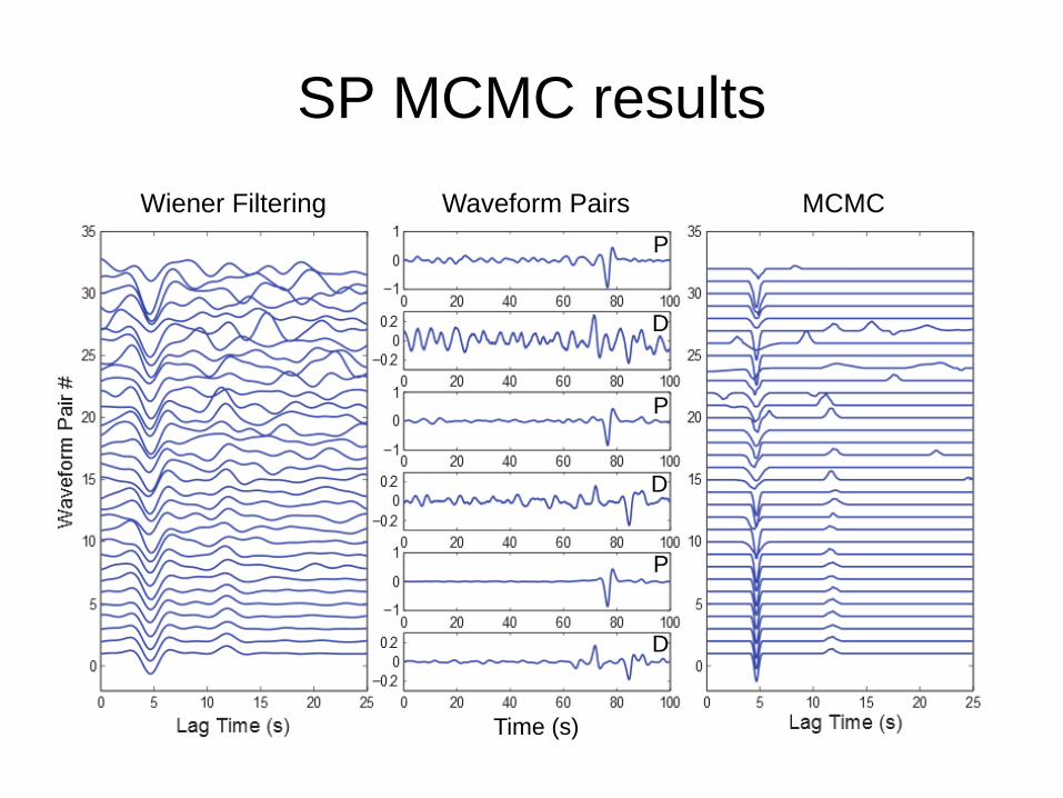
SP MCMC results
Wiener Filtering MCMC Waveform Pairs
Time (s)
P
P
P
D
D
D
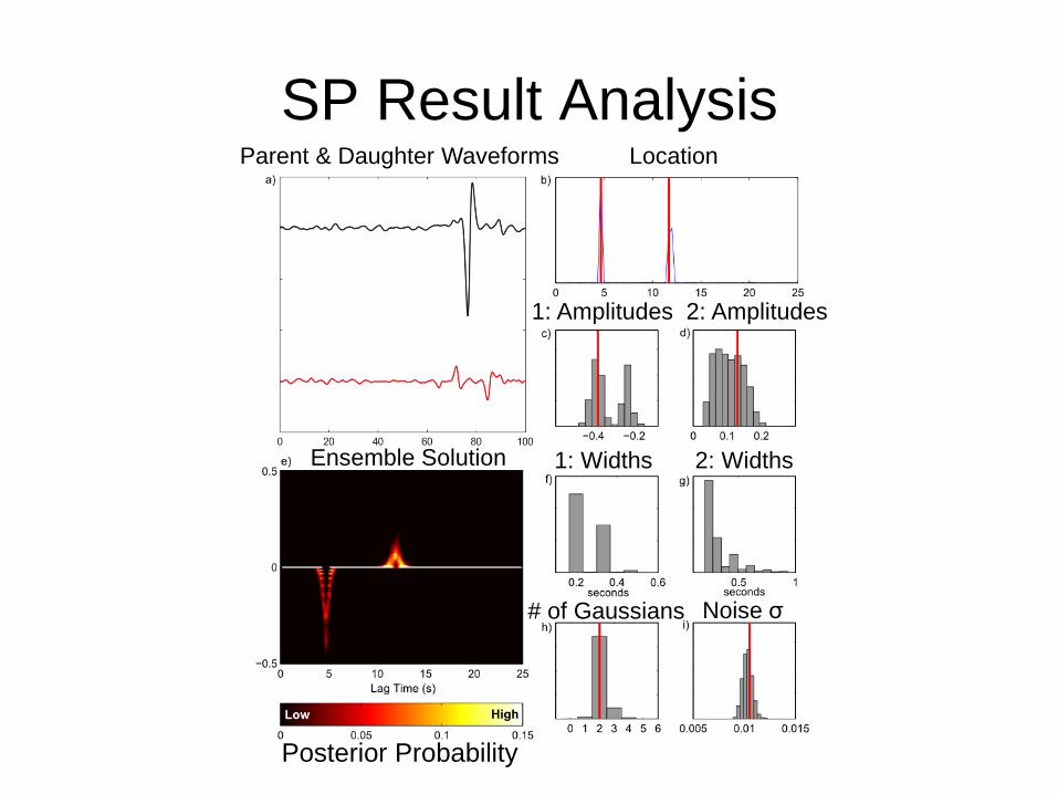
SP Result Analysis Parent & Daughter Waveforms Location
1: Amplitudes 2: Amplitudes
1: Widths 2: Widths
# of Gaussians Noise σ
Ensemble Solution
Posterior Probability
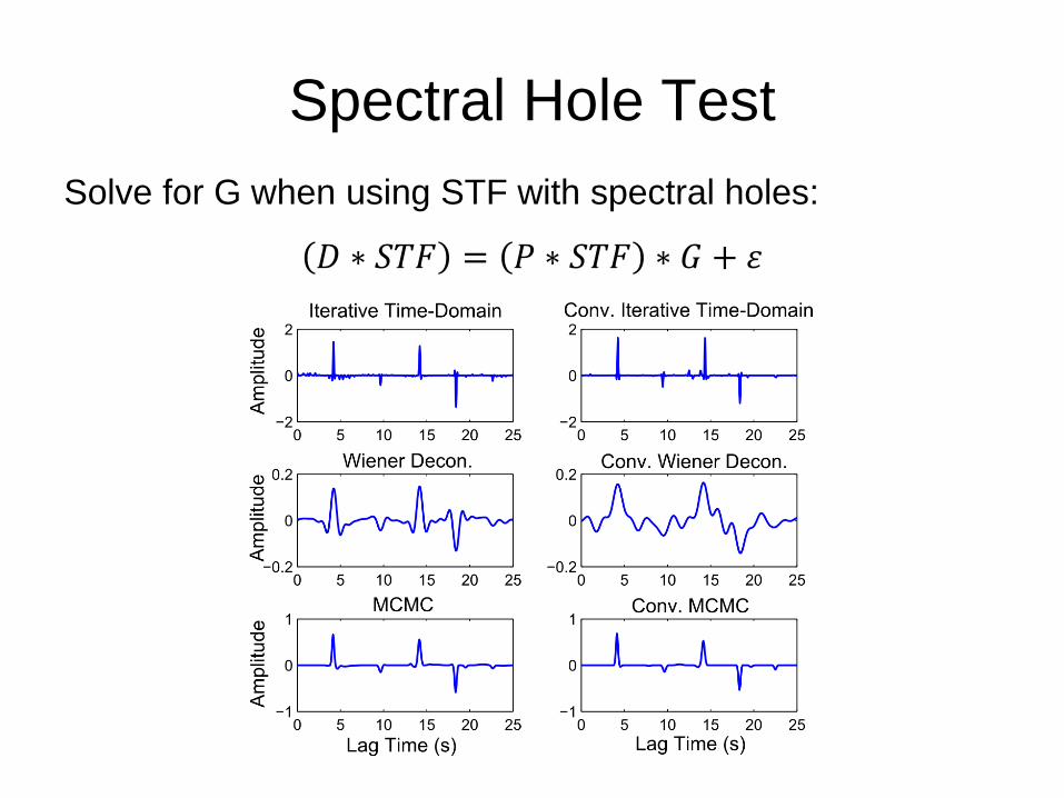
Spectral Hole Test
Solve for G when using STF with spectral holes:
𝐷 ∗ 𝑆𝑇𝐹 = 𝑃 ∗ 𝑆𝑇𝐹 ∗ 𝐺 + 𝜀
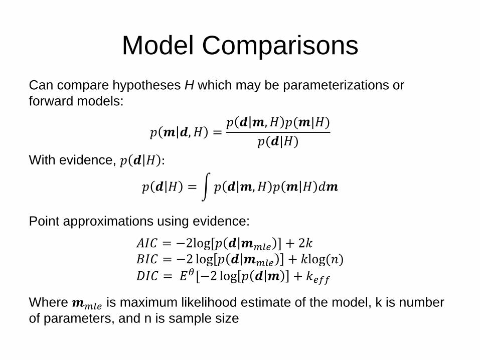
Model Comparisons
Can compare hypotheses H which may be parameterizations or
forward models:
𝑝 𝒎 𝒅,𝐻 =𝑝 𝒅 𝒎,𝐻 𝑝(𝒎|𝐻)
𝑝(𝒅|𝐻)
With evidence, 𝑝 𝒅 𝐻 :
𝑝 𝒅 𝐻 = 𝑝 𝒅 𝒎,𝐻 𝑝 𝒎 𝐻 𝑑𝒎
Point approximations using evidence:
𝐴𝐼𝐶 = −2log [𝑝 𝒅 𝒎𝑚𝑙𝑒 ] + 2𝑘
𝐵𝐼𝐶 = −2 log 𝑝 𝒅 𝒎𝑚𝑙𝑒 + 𝑘log(𝑛)
𝐷𝐼𝐶 = 𝐸𝜃[−2 log 𝑝 𝒅 𝒎 + 𝑘𝑒𝑓𝑓
Where 𝒎𝑚𝑙𝑒 is maximum likelihood estimate of the model, k is number
of parameters, and n is sample size
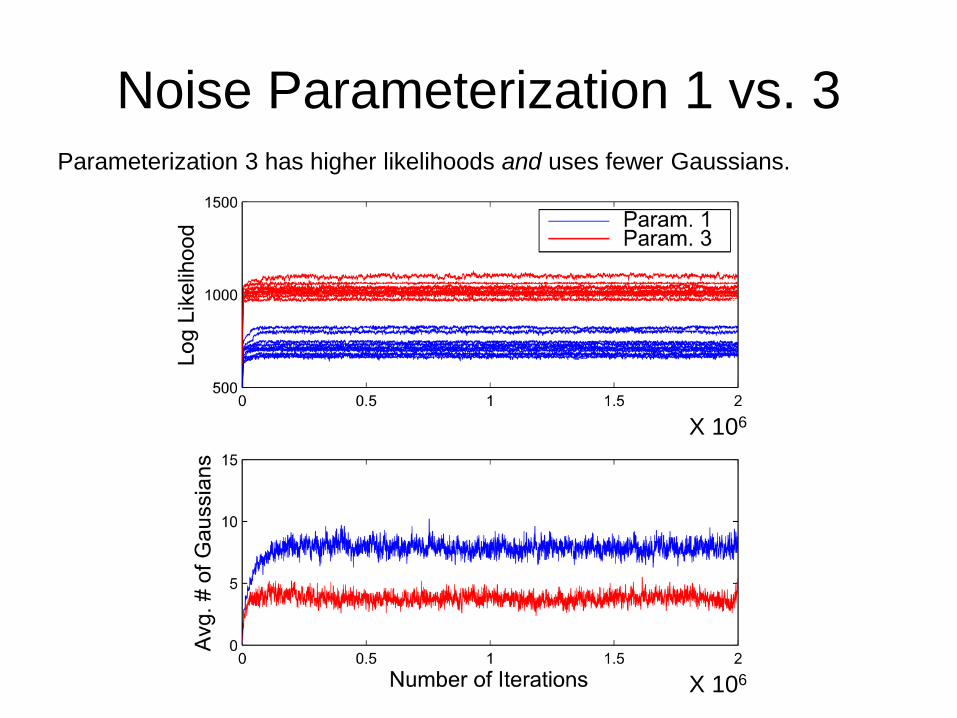
Noise Parameterization 1 vs. 3 Parameterization 3 has higher likelihoods and uses fewer Gaussians.
X 106
X 106
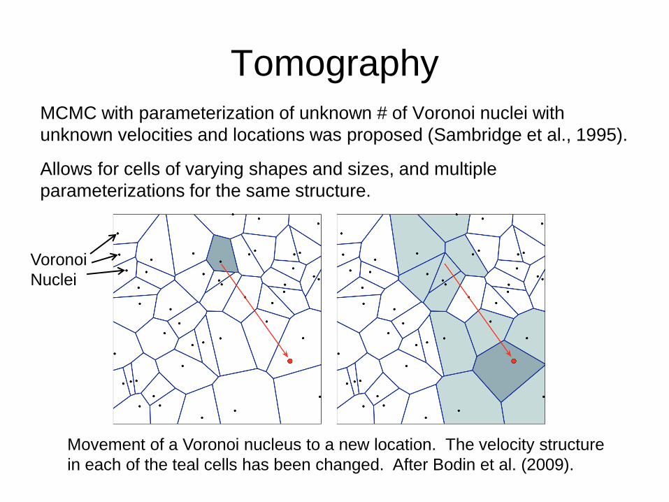
Tomography MCMC with parameterization of unknown # of Voronoi nuclei with
unknown velocities and locations was proposed (Sambridge et al., 1995).
Allows for cells of varying shapes and sizes, and multiple
parameterizations for the same structure.
Voronoi
Nuclei
Movement of a Voronoi nucleus to a new location. The velocity structure
in each of the teal cells has been changed. After Bodin et al. (2009).
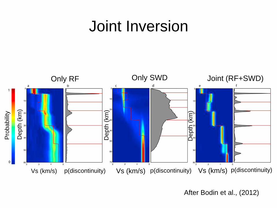
Joint Inversion
After Bodin et al., (2012)
Vs (km/s) Vs (km/s) p(discontinuity) p(discontinuity) Vs (km/s) p(discontinuity)
Only RF Only SWD Joint (RF+SWD)
Pro
babili
ty
Depth
(km
)
De
pth
(km
)
Depth
(km
)
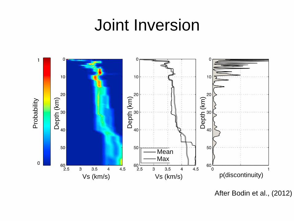
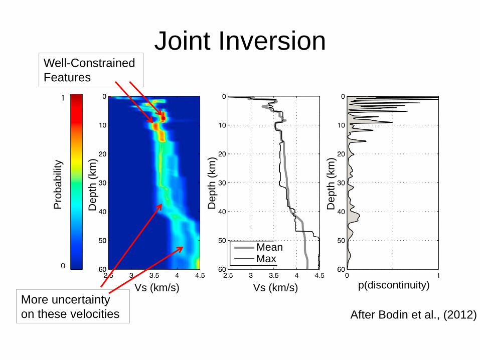
Joint Inversion
Vs (km/s) Vs (km/s) p(discontinuity)
Pro
ba
bili
ty
Depth
(km
)
Depth
(km
)
De
pth
(km
)
Mean Max
After Bodin et al., (2012)
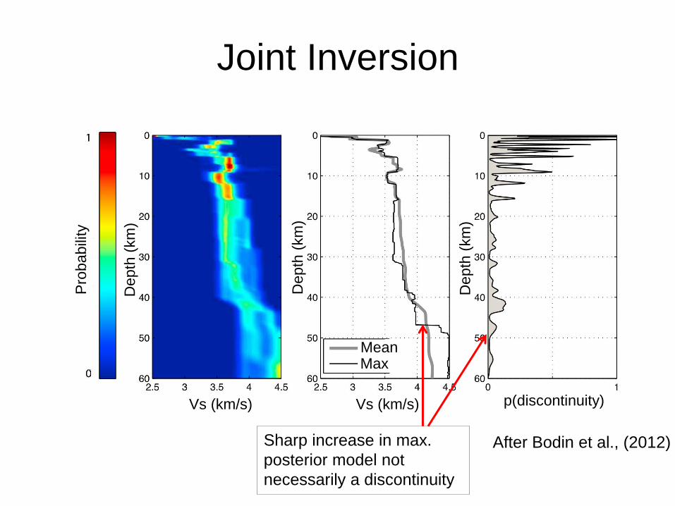
Joint Inversion
Vs (km/s) Vs (km/s) p(discontinuity)
Pro
ba
bili
ty
Depth
(km
)
Depth
(km
)
De
pth
(km
)
Mean Max
After Bodin et al., (2012)
Well-Constrained
Features
More uncertainty
on these velocities
Joint Inversion
Vs (km/s) Vs (km/s) p(discontinuity)
Pro
ba
bili
ty
Depth
(km
)
Depth
(km
)
De
pth
(km
)
Mean Max
After Bodin et al., (2012) Sharp increase in max.
posterior model not
necessarily a discontinuity
Conclusions
Transdimensional MCMC:
• Is a data-driven approach allowing for dimensionality to
be decided by the data;
• Results in an ensemble solution of models that can
make uncertainty analysis simpler;
• Provides uncertainties on individual features of solutions;
• Can jump out of local minima and can sample non-
unique solutions.
Acknowledgements
Vedran Lekic
Fellow “transdimensionalers”
CREWES
References
• Agostinetti, N. Piana, and A. Malinverno. "Receiver function inversion by
trans‐dimensional Monte Carlo sampling." Geophysical Journal International
181.2 (2010): 858-872.
• Bodin, Thomas, and Malcolm Sambridge. "Seismic tomography with the
reversible jump algorithm." Geophysical Journal International 178.3 (2009):
1411-1436.
• Bodin, Thomas, et al. "Transdimensional inversion of receiver functions and
surface wave dispersion." Journal of Geophysical Research: Solid Earth
(1978–2012) 117.B2 (2012).
• Jones, Gareth. Finance Markov Chain Example State Space. Digital image.
Wikipedia.org. Wikipedia, n.d. Web.
<http://en.wikipedia.org/wiki/File:Finance_Markov_chain_example_state_sp
ace.svg>.
• Sambridge, Malcolm (2010). “Uncertainty in Transdimensional Inverse
Problems.” PDF File. Lecture Slides.

Happy Valentine’s Day!


