1 Transfer Learning-Based Outdoor Position Recovery with Telco Data Yige Zhang, Aaron Yi Ding, J¨ org Ott, Mingxuan Yuan, Jia Zeng, Kun Zhang and Weixiong Rao Telecommunication (Telco) outdoor position recovery aims to localize outdoor mobile devices by leveraging measurement report (MR) data. Unfortunately, Telco position recovery requires sufficient amount of MR samples across different areas and suffers from high data collection cost. For an area with scarce MR samples, it is hard to achieve good accuracy. In this paper, by leveraging the recently developed transfer learning techniques, we design a novel Telco position recovery framework, called TLoc, to transfer good models in the carefully selected source domains (those fine-grained small subareas) to a target one which originally suffers from poor localization accuracy. Specifically, TLoc introduces three dedicated components: 1) a new coordi- nate space to divide an area of interest into smaller domains, 2) a similarity measurement to select best source domains, and 3) an adaptation of an existing transfer learning approach. To the best of our knowledge, TLoc is the first framework that demonstrates the efficacy of applying transfer learning in the Telco outdoor position recovery. To exemplify, on the 2G GSM and 4G LTE MR datasets in Shanghai, TLoc outperforms a non- transfer approach by 27.58% and 26.12% less median errors, and further leads to 47.77% and 49.22% less median errors than a recent fingerprinting approach NBL. I. I NTRODUCTION Recent years we have witnessed the ever-growing size and complexity of telecommunication (Telco) networks to process 1000-fold growth in the amount of traffic and 100- fold increase in the number of users [19]. Telco operators have to manage heterogeneous networks (including 2G-4G and upcoming 5G networks), composed of macro cells, small cells, and distributed antenna systems. The growing demands and heterogeneous networks require an automated approach to network control and management, instead of error-prone manual network management and parameter configuration. To enable the automated network control and management, the outdoor locations of mobile devices are important for Telco operators to 1) pinpoint location hotspots for capacity planning, 2) identify gaps in radio frequency spatial coverage, and 3) locate users in emergency situations (E911) [19]. Moreover, the locations of mobile devices are widely used to understand mobility patterns and optimize many third-party applications such as urban planning and traffic forecasting [6]. Yige Zhang and Weixiong Rao are with Tongji University, Shanghai, China. E-mail: {1610832, wxrao}@tongji.edu.cn Aaron Yi Ding is with the Department of Engineering Systems and Services at TU Delft, Netherlands. E-mail: [email protected]J¨ org Ott is with Technical University of Munich in the Faculty of Infor- matics. E-mail: [email protected]Mingxuan Yuan and Jia Zeng are with Huawei Noahs Ark Lab, Hong Kong. E-mail: {mingxuan.yuan, jia.zeng}@huawei.com Kun Zhang is with the CMU philosophy department as an assistant professor and an affiliate faculty member in the machine learning department. E-mail: [email protected]Outdoor locations of mobile devices can be recovered from Telco Measurement record (MR) data [9]. MR samples are generated when mobile devices make phone calls and access data services. MR samples contain connection states (e.g., signal strength) between mobile devices and connected base stations. After the locations of mobile devices are recovered, we tag the MR samples by the associated geo-locations, generating the so-called geo-tagged MR samples. In literature, various position recovery algorithms via Telco MR samples have been developed. Google MyLocation [2] approximates outdoor locations by the positions of cellular towers connected with mobile devices. This method suffers from median errors of hundreds and even thousands of meters. More recently, data-driven approaches have attracted intensive research interests in both academia and Telco industry [4], [13], [16], [28], [33], [37]. These approaches leverage geo- tagged MR samples to build the mapping from MR samples to associated locations, and the mapping is then used to localize the mobile devices in non-geo-tagged samples. For example, the fingerprinting approach [13] builds a histogram of MR signal strength (i.e., fingerprint database) for each divided grid cell in the areas of interest, and the Random Forest (RaF)- based approach [37] maintains the mapping function between MR features (i.e., MR signal strength) and position labels. When enough amount of training geo-tagged MR samples are used, the data-driven algorithms achieve the median error of 20 ∼ 80 meters [12], [37]. A key concern of the data-driven methods mentioned above is requiring sufficient geo-tagged MR samples to build the accurate mapping from MR samples to associated locations. Nevertheless, collecting sufficient geo-tagged MR samples across the distributed areas of an urban city incurs rather high cost. It is not rare that an area of interest suffers from insufficient geo-tagged MR samples. If we have scarce geo- tagged MR samples for such an area, the position recovery precision in that area could be very low. For example in a recent work NBL [19], though over 100 TB GPS-tagged Telco signal data in an American city are collected by 4 million users from Jan 2016 to July 2016, the median localization errors in rural areas are still as high as around 750 meters due to insufficient samples. In this paper, targeting Telco operators, we design a transfer learning-based Telco position recovery approach, called TLoc, to accurately localize mobile devices in those areas with scarce data samples. The general idea of TLoc is as follows. First, we divide an entire area into fine-grained small subareas, namely domains. For each domain, we then maintain the mapping from MR samples within this domain to their associated posi- tions. Next for the target domains suffering from low precision,
Transcript
1
Transfer Learning-Based Outdoor Position Recoverywith Telco Data
Yige Zhang, Aaron Yi Ding, Jorg Ott, Mingxuan Yuan, Jia Zeng, Kun Zhang and Weixiong Rao
Telecommunication (Telco) outdoor position recovery aimsto localize outdoor mobile devices by leveraging measurementreport (MR) data. Unfortunately, Telco position recovery requiressufficient amount of MR samples across different areas andsuffers from high data collection cost. For an area with scarce MRsamples, it is hard to achieve good accuracy. In this paper, byleveraging the recently developed transfer learning techniques,we design a novel Telco position recovery framework, calledTLoc, to transfer good models in the carefully selected sourcedomains (those fine-grained small subareas) to a target one whichoriginally suffers from poor localization accuracy. Specifically,TLoc introduces three dedicated components: 1) a new coordi-nate space to divide an area of interest into smaller domains,2) a similarity measurement to select best source domains, and3) an adaptation of an existing transfer learning approach. Tothe best of our knowledge, TLoc is the first framework thatdemonstrates the efficacy of applying transfer learning in theTelco outdoor position recovery. To exemplify, on the 2G GSMand 4G LTE MR datasets in Shanghai, TLoc outperforms a non-transfer approach by 27.58% and 26.12% less median errors, andfurther leads to 47.77% and 49.22% less median errors than arecent fingerprinting approach NBL.
I. INTRODUCTION
Recent years we have witnessed the ever-growing sizeand complexity of telecommunication (Telco) networks toprocess 1000-fold growth in the amount of traffic and 100-fold increase in the number of users [19]. Telco operatorshave to manage heterogeneous networks (including 2G-4Gand upcoming 5G networks), composed of macro cells, smallcells, and distributed antenna systems. The growing demandsand heterogeneous networks require an automated approachto network control and management, instead of error-pronemanual network management and parameter configuration.To enable the automated network control and management,the outdoor locations of mobile devices are important forTelco operators to 1) pinpoint location hotspots for capacityplanning, 2) identify gaps in radio frequency spatial coverage,and 3) locate users in emergency situations (E911) [19].Moreover, the locations of mobile devices are widely usedto understand mobility patterns and optimize many third-partyapplications such as urban planning and traffic forecasting [6].
Yige Zhang and Weixiong Rao are with Tongji University, Shanghai, China.E-mail: {1610832, wxrao}@tongji.edu.cn
Aaron Yi Ding is with the Department of Engineering Systems and Servicesat TU Delft, Netherlands. E-mail: [email protected]
Jorg Ott is with Technical University of Munich in the Faculty of Infor-matics. E-mail: [email protected]
Mingxuan Yuan and Jia Zeng are with Huawei Noahs Ark Lab, Hong Kong.E-mail: {mingxuan.yuan, jia.zeng}@huawei.com
Kun Zhang is with the CMU philosophy department as an assistantprofessor and an affiliate faculty member in the machine learning department.E-mail: [email protected]
Outdoor locations of mobile devices can be recovered fromTelco Measurement record (MR) data [9]. MR samples aregenerated when mobile devices make phone calls and accessdata services. MR samples contain connection states (e.g.,signal strength) between mobile devices and connected basestations. After the locations of mobile devices are recovered,we tag the MR samples by the associated geo-locations,generating the so-called geo-tagged MR samples.
In literature, various position recovery algorithms via TelcoMR samples have been developed. Google MyLocation [2]approximates outdoor locations by the positions of cellulartowers connected with mobile devices. This method suffersfrom median errors of hundreds and even thousands of meters.More recently, data-driven approaches have attracted intensiveresearch interests in both academia and Telco industry [4],[13], [16], [28], [33], [37]. These approaches leverage geo-tagged MR samples to build the mapping from MR samples toassociated locations, and the mapping is then used to localizethe mobile devices in non-geo-tagged samples. For example,the fingerprinting approach [13] builds a histogram of MRsignal strength (i.e., fingerprint database) for each divided gridcell in the areas of interest, and the Random Forest (RaF)-based approach [37] maintains the mapping function betweenMR features (i.e., MR signal strength) and position labels.When enough amount of training geo-tagged MR samples areused, the data-driven algorithms achieve the median error of20 ∼ 80 meters [12], [37].
A key concern of the data-driven methods mentioned aboveis requiring sufficient geo-tagged MR samples to build theaccurate mapping from MR samples to associated locations.Nevertheless, collecting sufficient geo-tagged MR samplesacross the distributed areas of an urban city incurs ratherhigh cost. It is not rare that an area of interest suffers frominsufficient geo-tagged MR samples. If we have scarce geo-tagged MR samples for such an area, the position recoveryprecision in that area could be very low. For example in arecent work NBL [19], though over 100 TB GPS-tagged Telcosignal data in an American city are collected by 4 million usersfrom Jan 2016 to July 2016, the median localization errorsin rural areas are still as high as around 750 meters due toinsufficient samples.
In this paper, targeting Telco operators, we design a transferlearning-based Telco position recovery approach, called TLoc,to accurately localize mobile devices in those areas with scarcedata samples. The general idea of TLoc is as follows. First, wedivide an entire area into fine-grained small subareas, namelydomains. For each domain, we then maintain the mappingfrom MR samples within this domain to their associated posi-tions. Next for the target domains suffering from low precision,
2
we transfer good mappings from appropriately selected sourcedomains to target ones via transfer learning. In this way, wegreatly improve the localization accuracy in target domains.Though transfer learning has been used for indoor WiFi-basedlocalization [21], [34], [35], we believe that indoor WiFi andoutdoor Telco localization differs significantly. Thus, thoseindoor localization approaches are not expected to performwell in our case (they will be evaluated in our experiment)due to the following challenges. Firstly, given the outdoorTelco localization, designing a proper position coordinatespace is the prerequisite to enable knowledge transfer acrosstwo domains. This, unfortunately, cannot be achieved by usingoutdoor GPS longitude and latitude coordinates: the differentGPS position (i.e., position label) for every area makes itimpossible to share position labels across distributed domains,and hence hard to perform knowledge transfer. Secondly, givena large number of domains, it is challenging to select the bestsource domains for a target one. In contrast, due to the smallarea and rather limited domains in an indoor environment,it is straightforward for indoor localization to select sourcedomains. Thus, trivial effort on source domain selection isemployed for indoor WiFi-based localization [21], [34], [35].
To tackle the challenges above, TLoc builds the followingcomponents. Firstly, unlike absolute GPS coordinates, we usea relative coordinate space for position recovery. Under thiscoordinate space, the mobile devices even in two distributeddomains can still share the same relative positions, facili-tating the transfer across two domains. Secondly, based onthe relative position space, we design an effective distancemetric to measure the similarity between domains. The metricincorporates the distribution of the signal strength of MRsamples, relative position information, and non-serving basestation deployment information. Finally, by adapting an exist-ing structured transfer learning (STL) method [25], we build aRandom Forest (RaF)-based position recovery model for eachdomain and then perform model transfer from appropriatelychosen source domains to target ones. As a summary, thispaper makes the following contributions.
• To the best of our knowledge, TLoc is the first methodto plausibly leverage transfer learning for Telco outdoorlocalization. Unlike the fingerprinting-based and machinelearning-based approaches [12], [16], [37], TLoc miti-gates high efforts to collect a large quantity of trainingsamples across an entire area. Moreover, our evaluationempirically verifies that the idea of TLoc can gener-ally benefit other approaches (e.g., fingerprinting-basedapproaches) to achieve better precision by re-using MRsamples from source domains to target ones.
• We design a novel approach to divide an entire urbanarea into small domains by the proposed relative coordi-nate space. Based on the divided domains, we define adistance metric for measuring domain similarity to selectappropriate source domains effectively for a target one.By adapting a recent structured transfer learning (STL)scheme [25] for a RaF regression model [37], TLoc leadsto much better position recovery precision than those non-transfer models.
• Our extensive evaluation validates that TLoc greatlyoutperforms both state-of-the-arts and the variants ofTLoc. For example, on two 2G GSM and 4G LTEMR datasets, TLoc outperforms the recent fingerprintingapproach NBL [19] by 47.77% and 49.22% less medianerrors, respectively, and leads to 27.58% and 26.12% lessmedian error when compared with the non-transfer RaFalgorithm [37], respectively.
The rest of this paper is organized as follows. Section IIreviews the background and related work. Section III givesthe general idea of TLoc and the proposed relative coordinatespace. After that, Section IV defines the distance metric tomeasure domain similarity, and Section V adapts the STLmodel [25] for TLoc. Section VI evaluates TLoc and SectionVII finally concludes the paper. Table I summarizes the mainacronyms and notations used in the paper.
Notation/Symbol MeaningTelco TelecommunicationMR Measurement ReportTL Transfer LearningSTL Structure Transfer LearningSVR Supported Vector RegressionRSSI Received Signal Strength IndicatorRaF Random Forest
D, s Domain (divided small areas), MR SampleST and SS Target and Source Data SetFd(), Fi() MR Features dependent (resp. independent) upon locationsL() Recovered Locationdisrssimr , dissigmr Weighted Histogram Distance of RSSI (resp. SignalLevel)dismr Overall MR Feature Distancedispos Relative Position Distancedist(D,D′) Domain Distance between two domains D and D′
TABLE IMAINLY USED SHORT NAMES/SYMBOLS AND NOTATIONS.
II. BACKGROUND AND RELATED WORK
In this section, firstly we give the background of Mea-surement Report (MR), Random Forests (RaF), and transferlearning, and secondly review the literature in terms of outdoorposition recovery and selection of source domains.
TABLE IIA 2G GSM MR SAMPLE COLLECTED BY AN ANDROID DEVICE.
Measurement Report (MR) Data: MR samples are usedto record the connection states between mobile devices andnearby base stations in a Telco network. Table II gives anexample of 2G GSM MR samples collected by an Android de-vice. It contains a unique number (IMSI: International MobileSubscriber Identity), connection time stamp (MRTime), up to7 nearby base stations (identified by RNCID and CellID) [24],signal measurements such as AsuLevel and SignalLevel, anda radio signal strength indicator (RSSI). SignalLevel indicatesthe power ratio (typically logarithm value) of the output signalof the device and the input signal. AsuLevel, i.e., Arbitrary
3
Strength Unit (ASU), is an integer value proportional tothe received signal strength measured by the mobile phone.Among the up-to 7 base stations, one of them is selected asthe primary serving base station to provide communicationand data transmission services for the mobile device. Previouswork on Telco localization [12], [37] might ignore the useof serving base station. Unlike these works, we will carefullyexploit serving base stations as the base of TLoc.
Besides 2G GSM MR samples, we also collect 4G LTEMR samples by frontend Android devices. They both followthe same data format. Nevertheless, due to the limitation ofAndroid API, frontend Android devices cannot acquire theidentifiers (RNCID 2 ∼ 7 and CellID 2 ∼ 7) of non-servingbase stations from 4G LTE networks. Nevertheless, the signalmeasurements associated with the missed base stations can bestill collected.
Finally, Telco operators can collect MR samples via back-end base stations except the frontend MR samples aboveby Android mobile phones. Nevertheless, their data formatsare different [12]. Firstly, besides RSSI, the backend 4GMR samples provided by Telco operators contain RSRP andRSRQ which do not appear in the frontend 4G MR samples.Secondly, backend 2G MR samples contain RxLev, the re-ceived signal strength on ARFCN (Absolute Radio FrequencyChannel Number) [12]. The previous work [11] shows thatRxLev is exactly equal to the RSSI value, and we thus treatRxLev equally as RSSI. Now, to make sure that we haveproper knowledge transfer between frontend and backend MRdatasets, we perform knowledge transfer only for those MRfeature items (e.g., RSSI) that appear within all datasets.For example, we transfer the knowledge from the RSSI (orRxLev) items in backend 2G MR samples to the RSSI itemsin frontend 2G samples. Yet, we do not transfer knowledgefor such MR features as RSRP and RSRQ.
Random Forest (RaF) is an ensemble method for clas-sification, regression, and other learning tasks. It constructsa multitude of decision trees (DTs) [1] during the trainingphase and outputs either the class that is the mode of theclasses (classification) or mean prediction (regression) of theindividual trees. RaF avoids the overfitting of DTs to theirtraining set. Specifically, DTs that are grown very deep tendto learn highly irregular patterns: they overfit their trainingsets, i.e., low bias but very high variance. RaFs are a wayof averaging multiple deep DTs, trained on different parts ofthe same training set, with the goal of reducing the variance.This greatly boosts the performance in the final model, atthe expense of a small increase in the bias and loss ofinterpretability.
Transfer learning aims at improving the learning in anew task through proper transfer of knowledge from a relatedtask that has already been learned. Those machine learningalgorithms such as RaFs are designed to address a single task.In contrast, transfer learning attempts to leverage individualtasks by developing methods to transfer knowledge learnedin one or more source tasks to a related target task. Transferlearning is frequently used due to expensive cost or impos-sibility to re-collect the needed training data and rebuild themodels. Transfer learning approaches include Model Transfer,
Instance Transfer (or data sample transfer), Features Transfer,and Relational knowledge-Transfer. We refer interested readersto the detailed survey of transfer learning [22].
TLoc mainly utilizes a recent model transfer scheme, i.e.,the structure transfer learning (STL) [25] in decision tree(DT)-based model to transfer knowledge from multiple sourcedomains to the target one. Specifically, DTs for similar prob-lems (in various domains) exhibit a certain extent of structuralsimilarity. However, the scale of the features used to constructRaF and their associated decision thresholds are likely todiffer from various problems. Thus, the DTs trained on sourcedomains are adapted to the target one by discarding all numericthreshold values in the original DTs and working top-down,and then selecting a new threshold for a node with a numericfeature using the subset of target examples that reach this node.
Recall that general transfer learning frameworks (such asinstance transfer) require training examples from source do-mains for domain adaptation. Instead, the STL scheme candirectly adapt the already trained models from source domainsto target ones. This unique property is particularly useful forthe scenario that cannot directly leverages source examples fordomain adaption, for whatever reason, e.g., storage capacityor data privacy. Thus, TLoc can comfortably adapt a givensource model to a target domain relying on a relatively smalltraining set from the target. The experimental results show thatmulti-source transfer in STL has the better precision than thesingle-source transfer.
Outdoor position recovery: In the literature, Telco out-door position recovery techniques are broadly classified intotwo categories: 1) measurement-based methods [17], 2) data-driven methods. Measurement-based methods frequently adoptabsolute point-to-point distance estimation or angle estima-tion from Telco signals to calculate mobile device locations.Examples of measurement-based techniques include Angle ofarrival (AOA), Time of Arrival (TOA) [8], and Received signalstrength (RSS)-based single source localization [29]. Never-theless, information related to AOA and TOA is highly errorprone in cellular systems, and measurement-based techniquessuffer from high localization errors, typically with the medianerror of hundreds of meters [8], [23]. In addition, as shownin previous work [23], 4G LTE MR samples typically havesignal strength from at most two cells, namely, the servingcell and the strongest neighboring cell. Triangulation-basedlocalization approaches thus do not perform well because theyrequire signal strength from at least three cells.
Fingerprinting-based and machine learning-based algo-rithms generally belong to the data-driven methods. Theyboth leverage collected historical data samples for outdoorposition recovery. Fingerprinting methods [13], [16] have beenreported to have better performance than measurement-basedapproaches. For example, in the offline survey phase, theclassic work, CellSense [13], first divides the area of interestinto smaller cells and constructs a fingerprint database, e.g., avector histogram of RSSI on each cell. When given a query(i.e., an input RSSI feature), the online prediction phase thensearches the fingerprint database to find the location that hasthe maximum probability given the received signal strengthvector in the query. An average of the k most probable
4
fingerprint cells, weighted by the probability of each location,can be used to obtain a better estimate of locations. In addition,a better CellSense-hybrid technique consists of two phases: therough estimation phase first uses the standard probabilisticfingerprinting technique to obtain the most probable cell inwhich a user may be located, and the estimation refinementphase then uses a k-nearest neighbor approach to estimate theclosest fingerprint point, in the signal strength space, to thecurrent user location inside the cell estimated in phase one.
AT&T researchers recently studied the fingerprinting-basedoutdoor localization problems [23], [19]. In particular, theauthors in NBL [19] extended CellSense [13] similarly usingtwo stages. In an offline stage, NBL developed radio frequencycoverage maps based on a large-scale crowdsourced channelmeasurement campaign. Then, in an online stage, a local-ization algorithm quickly matches the input radio frequencymeasurements to coverage maps. By assuming a Gaussiandistribution of signal strength within each divided grid, NBLmaintains the mean value and standard deviation of signalstrength of each neighboring cell tower for the samples inthe grid. The online stage computes the predicted locationby using either Maximum Likelihood Estimation (MLE) orWeighted Average (WA). The median errors in the 4G LTEnetwork reported by NBL are around 80 and 750 meters inurban and rural areas, respectively.
Machine learning approaches leverage machine learningmodels such as Random Forests, Support Vector Regression(SVR), Gradient Boosting Decision Tree (GBDT), and artifi-cial neural network (ANN) to build the mapping from MR fea-tures (which are extracted from MR samples and engineeringparameter data of connected base stations) to device positions[37], [12]. When given an MR record without position infor-mation, machine learning models then predict the associatedlocation. As shown in [37], the authors proposed a context-aware coarse-to-fine regression (CCR) model (implementedby a two-layer RaFs). The CCR model takes as input 258dimensional coarse features and 34 dimensional fine-grainedcontextual feature vectors. Thus, beyond strength indicatorsfrequently used by fingerprinting approaches, those context-aware and coarse-to-fine features such as moving speed enableCCR to outperform the classic fingerprinting approaches withslightly 14% lower median errors. In a very recent deeplearning-based outdoor cellular localization system, namelyDeepLoc [26], a data augmentor is used to handle data noiseissue and to provide more training samples. With help ofthe samples, a deep learning model is trained for betterlocalization result.
Source Domain Selection: Given a number of diversesource domains, to successfully perform knowledge transfer,one may need to select a certain number of source domainsthat bear essential similarity to the considered target do-main. Some previous works in transfer learning studied thegeneral source domain selection problem. For example, aninformation theoretic framework was developed [3] to ranksource convolution neural networks (CNNs) and select thetop-k CNNs for the target learning task by understandingthe source-target relationship. A restricted boltzman machine(RBM) was also used [5] to select source domains in the
context of reinforcement learning. Some works instead did nottake domain selection into account and focused on instanceselection from available source domains [18]. In addition,many existing transfer learning methods suppose that sourcedomains are provided in advance by default.
Compared to the above methods, TLoc gives a meaningfuldistance metric to determine the domain similarities for Telcoposition recovery task. Unlike TLoc, the previous work [3]focuses on the selection of pre-trained CNN models whichcan be intuitively treated as learning tasks, and [18] selectssource instances.
III. SYSTEM DESIGN
A. General Idea
We first give the general idea of TLoc to perform modeltransfer across different domains. In Figure 1, we considerthat two mobile devices m and m′ in two distributed domainsD and D′ (with D 6= D′) generate the MR samples s ands′, respectively. Suppose that we are using a RaF regressionmodel to recover the outdoor locations L(s) and L(s′) forthe samples s and s′, respectively. The outdoor locations arefrequently represented by GPS coordinates [12], [19], [23],[37]. Given the two distributed domains D 6= D′, the MRsamples s and s′ within the two domains indicate that thecorresponding RNC/CellID and GPS positions are different,indicating s 6= s′ and L(s) 6= L(s′).
D D’
MR Samples
Outdoor Positionm m’
Position Recovery
s s’
L(s) L(s’)
Domain
F (s)i F (s’)i
F s)d F s’)d((
Fig. 1. General Idea of TLoc
Inside MR samples, we note that there exist two typesof features: 1) those ID-alike features Fd() dependent uponlocated domains such as RNCID and CellID, and 2) thosenumeric features Fi() independent upon located domains suchas AsuLevel, SignalLevel and RSSI. Due to the distributeddomains D and D′, Fd(s) 6= Fd(s
′) holds. Nevertheless,when the two samples s and s′ contain very similar Telcosignal strength (including AsuLevel, SignalLevel and RSSI),it is highly possible to have Fi(s) ' Fi(s
′). The similarTelco signal strength gives us a hint: we would like to modifythe representation of the features Fd() and locations L() toensure that Fd(s) ' Fd(s
′) and L(s) ' L(s′) hold. Whenboth Fi(s) ' Fi(s′) and Fd(s) ' Fd(s′) hold, we then couldhave the similar MR samples s ' s′ and the roughly equalpositions L(s) ' L(s′). Based on this representation, we nextperform knowledge transfer across two similar MR sampless ∈ D ' s′ ∈ D′ as follows: if s ' s′ holds, we estimatethe position L(s)← L(s′) via the position L(s′). In general,we extend the idea of TLoc from similar samples to similardomains. Gvien the two similar domains D ' D′, we infers ∈ D ' s′ ∈ D′, and then estimate L(s) ← L(s′) via theavailable position L(s′).
5
B. Relative Coordinate Space
To perform the knowledge transfer above, we introduce arelative coordinate space to represent L() and Fd(), such thatFi(s) ' Fi(s
′) and Fd(s) ' Fd(s′) hold for two samples s
and s′ within two distributed domains D and D′.1) Representation of L(): We first represent L() by trans-
forming original GPS coordinates to relative coordinates asfollows. For the MR samples having a certain base stationas their serving stations, the mobile devices generating suchMR samples are highly possible to be located around theserving base station. Thus, based on serving base stations, wedivide a large urban area of interest (e.g., either a universitycampus or an entire city) into fine-grained small subareas (orequivalently we use the term domains D that are frequentlyused in the transfer learning community). That is, based onserving base stations in MR samples, the MR samples havingthe same serving base stations belong to the same domains.For every domain, we design a relative coordinate space forall MR samples within the domain. We use Figure 2 as anexample to represent the relative coordinates. In this figure,we assume that those MR samples belonging to the samedomain D (a.k.a having the same serving base station BS)are all within a circle and BS is the center. The radius Rof this circle is equal to the maximal distance between thepositions of BS and MR samples. Given this center BS inthe coordination space, we convert the original GPS coordinate(x0, y0) of BS into a relative one (0, 0). For a MR samples ∈ D with the GPS coordinate (x + x0, y + y0), its relativecoordinate becomes (x, y). In this way, we can compute therelative coordinates of all MR samples by referring BS as thecenter of this coordination space.
Until now, we show the key point of the relative coor-dination space as follows. Let us consider another domainD′, where the GPS position of the serving base station (i.e.,the center) belonging to D′ is (x1, y1). For one MR samples′ ∈ D′ with the GPS coordinate (x+ x1, y+ y1), its relativecoordinate becomes (x, y). Here, though the two sampless ∈ D and s′ ∈ D′ are originally with different GPScoordinates (x + x0, y + y0) and (x + x1, y + y1), they nowshare the exactly same relative coordinates (x, y) under theirown domains. In this way, we can perform the transfer fromD to D′. That is, when both Telco signal strength in MRsamples (a.k.a MR features) and relative position (labels) referto serving base stations, the transfer across domains becomespossible. Moreover, for a large amount of MR samples acrossan entire area, we can group the MR samples by their servingbase stations to build the associated domains and relativecoordination space. After the big area is divided into smalldomains, for each domain (and the associated serving basestation), we can learn an individual mapping from MR sampleswithin this domain to their relative positions. The key is thatthe mapping is adaptively learned by the data-driven fashion,even if the transmitting power, Telco signal coverage, andbandwidth of serving base stations are unavailable. Thus, evenfor two base stations (with various transmitting power, Telcosignal coverage, and bandwidth) located at the exactly samelocations, we could establish two corresponding mappings
from the MR samples generated by an individual base stationto the associated MR positions.
Note that the relative coordinate space above requires theGPS coordinate of serving base stations. Telco operators caneasily obtain the GPS coordinates of base stations becausebase stations are deployed by Telco operators themselves.
1 2 3 4 5 6 7 8 9 10
1
2
3
4
5
6
7
8
9
10
Locations of Neighbor
base stations in
(except serving BS)
Locations of MR
samples in
:
:
:
Fig. 2. Relative Coordinate Space
2) Representation of Fd(): For a certain MR sample s,we convert MR features Fd(s), such as RNCID and CellIDof a neighboring base station, into meaningful IDs whichare independent upon the associated domains. Specifically,depending upon all the neighbouring base stations appearinginside the MR samples within a domain, we determine arectangle area covered by these neighboring base stations. Asshown in Figure 2, the width (resp. height) of the rectangular isequal to 2×max(|xbsi |) (resp. 2×max(|ybsi |)), where we havemax(|xbsi |) = xbs1 and max(|ybsi |) = ybs5 . Then, we evenlydivide the rectangle into g × g small grids (we have g = 10in this figure). In this way, each neighboring base station islocated within a certain grid and we replace its RNCID andCellID by the associated grid IDs Grid IDx and Grid IDy . Forexample, we represent the two base stations bs1 and bs5 bythe grid IDs (1, 9) and (8, 1), respectively. The representationof Fd(s) above offers the following advantage: the grid IDsare now independent upon domains and Fd(s) ' Fd(s′) holdsfor two MR samples s ∈ D and s′ ∈ D′.
C. System Overview
InaccurateLocalization
Traditional position recovery
ComputingDomainDistance
Target Domains
Source Domains
Knowledge Transfer (STL)
Transfer Learning-based position recovery
Precise Positions
Random Forest Regression
TestingMR
Samples
TrainingMR
SamplesDomain Distance Matrix
Base Station
Database
Fig. 3. System Overview
Following the general idea above, we introduce three fol-lowing components of TLoc (see Figure 3): a traditionalposition recovery model (e.g., a Random Forest-based re-gression model), a matrix to maintain the pairwise domainsimilarity, and the transfer learning component for those target
6
domains suffering from inaccurate position accuracy (causedby insufficient position labels for MR training samples).
Let us consider the following scenario in a big area, wherethe geo-tagged MR samples are distributed unevenly acrossthis area. To this end, we follow Section III-B to divide theentire big area into multiple smaller areas (a.k.a domains) andrepresent MR samples and associated positions under the asso-ciated relative coordinate space. Among the divided domains,due to the uneven distribution of geo-tagged MR samples,some of the domains could be with sufficient samples, anda regression-based position recovery model thus works verywell. Yet other domains may contain scarce geo-tagged MRsamples, the trained position recovery model usually suffersfrom poor localization accuracy [12].
To this end, TLoc adapts the recent transfer learning schemeSTL [25] to improve the localization accuracy in the domainssuffering from poor prediction precision, e.g., with a medianerror higher than a given threshold. We treat such domainsas target domains. Based on the developed distance metric(Section IV), we choose those top-k domains that 1) are mostsimilar to a target domain and 2) are with low localizationerrors. Such top-k domains are called the source domains ofthe target one. Finally, we transfer the recovery models fromthe top-k source domains to the target one using an adaptedSTL technique (Section V).
IV. DOMAIN DISTANCE
Since the position recovery model essentially maintains themapping from MR features, e.g., Fi(s) and Fd(s), to MRpositions L(s), we thus define the domain distance by twoparts: 1) the distance in terms of MR features and 2) thedistance in terms of MR positions L(s). In this section, wefirst give the detail for each of the two parts and next give thedomain distance by integrating the two parts.
A. MR Feature Distance
To measure the similarity of MR features between twodomains, the distance metric takes into account three followingaspects: 1) the general approach to compute the distance ofthose MR features Fi(s) involving Telco signal strength, 2) thedistance by introducing the weight of up to seven base stations,and 3) the overall distance involving the refinement of threespecific signal strengths (RSSI, AsuLevel and SignalLevel).
1) Distance of Telco Signal StrengthFirstly, to compute the distance of Telco signal strength
between two domains, we exploit a histogram structure tocapture the overall distribution of Telco signal strength ina certain domain, and next compute the histogram distance.Figure 4 plots the histograms of two example domains tocapture the distribution of RSSI from serving base stations.The x-axis is the RSSI value and y-axis indicates the ratioof the MR samples having RSSI values falling inside aRSSI interval against total MR samples in the domain. Tocompute the histogram distance, we choose three frequentlyused metrics: probabilistic likelihood [32], [13], Kullback-Leibler Divergence [20], and p-norm distance [30]. Amongthe three metrics, we empirically find that the p-norm distance
with p = 3 leads to the best result. Formally, for a domain D(resp. D′), we denote by hD,j (resp. hD′,j) the MR samplerate in y-axis for the j-th RSSI interval in x-axis. Wheneach histogram contains r RSSI intervals, we compute thehistogram distance between D and D′ by
dishist(D,D′) = (
r∑j=1
(|hD,j − hD′,j |)p)1p (1)
Fig. 4. Histograms of Two Domains in terms of RSSI from Serving BaseStation (where 5198 indicates RNC ID and 16058/42507 indicates Cell ID)
2) Weighted Distance of Telco Signal StrengthWe note that each MR sample contains up to seven base
stations sorted by descending order of Telco signal strength.These stations contribute differently to the distance in Equation(1), due to various signal strength caused by these stations.
)
(a)(b)
( )( )
(d)(c)
Fig. 5. Distance of BS Locations between Domains
Specifically, each domain D contains a set of MR samples.For all (neighboring) base stations appearing in these MRsamples, we group such stations by their order index in MRsamples: the 1st group contains only one serving base stationwith the strongest signal strength, the 2nd group contains theneighboring base stations of 2nd order index (i.e., RNCID 2,CellID 2) in each MR sample. In this way, we have up toseven groups of base stations. Each group contains a list ofbase stations, denoted by li with i = 1, ..., 7. In this way, weimprove Equation (1) by introducing a weight wi for each li.
dismr(D,D′)=
7∑i=1
wi×disihist(D,D′) (2)
In Equation (2), disihist(D,D′), computed by Equation (1),
is the histogram distance for the Telco MR signal associatedwith the i-th lists li(D) and li(D′) in two domains D and D′,and wi is the weight of the i-th group.
We give the general idea of computing the weight wi asfollows. Recall that Section III-B transforms the neighboringbase stations (identified by RNCID and CellID) into gridIDs. Such grid IDs approximate the positions of neighboringstations within each domain: the nearest (resp. farthest) base
7
stations contribute to the strongest (resp. weakest) Telco signalstrength. We leverage these grid IDs to compute the weightwi. As shown in Figure 5, we have the 2nd base stationlists in two domains D and D′, denoted by l2(D) andl2(D
′), which contain 4 member stations bs2,1...bs2,4 and3 stations bs′2,1...bs
′2,3, respectively. Based on the distance
disi=2bs (D,D′) of the two lists l2(D) and l2(D′), , we define
the normalized weight wi as follows.
wi =edis
ibs∑7
j=1 edis
jbs
(3)
To compute the item disibs above, as shown in Figure 5(c),we exploit the average position of the 4 stations in l2(D),denoted by (xbsi , ybsi), and one of the 3 stations in l2(D
′),denoted by (xbs′i , ybs′i). After that, we compute the Euclideandistance between the two average positions.
disibs(D,D
′) = [(xbsi
− xbs′i)2+ (ybsi − ybs′i )
2]12 (4)
Nevertheless, the average positions above might lose thegeographical characteristics of base stations. Thus, as animprovement to compute the item disibs, as shown in Figure5(d), we first calculate the pairwise distance between the basestations in li(D) and li(D′), and then compute the average ofthe pairwise distance:
disibs(D,D
′) =
∑|li(D′)|
n=1
∑|li(D)|m=1 ed(bsi,m, bs
′i,n)
|li(D)||li(D′)|(5)
In Equation (5), ed(·) indicates the Euclidean Distance of twobase stations bsi,m and bs′i,n, whose positions are representedby grid IDs under the relative coordinate space.
Note that the 4G LTE MR samples collected by AndroidAPI may miss the IDs of neighbour base stations (see SectionII), and we cannot leverage the positions of base stations,required by Equation (5), to compute the weight wi. To over-come this issue, we could approximate wi =
1/i∑7j=1 1/j
, suchthat wi is inverse to the index number i. This approximationmakes sense: the index number i essentially indicates thesignal strength of base stations, and the weight w1 regardingto the 1st index (i.e., the serving base station) consequentlycontributes most to the overall distance.
3) Overall Distance of MR FeaturesThirdly, recall that MR samples in Table II contain three
types of signal strength: RSSI, AsuLevel and SignalLevel.For such signal strength, we might first follow Equation(2) to compute three associated histogram distance such asdisrssimr (D,D′) and next sum the three weighted distance asthe overall distance. However, the sum may not provide asensible overall measure if the three types of Telco signalstrength are heavily dependent. In fact this is the case becauseAsuLevel is a scaling value of RSSI, i.e., in 2G GSM data set,AsuLevel = (RSSI+113)/2 [24], and disasumr can be treatedas a linear transformation of disrssimr . Among the three typesof signal strength, we thus take into account the independentcontribution of RSSI and SignalLevel to compute the overalldistance of MR features.
In terms of SignalLevel, we follow Equation (2) to computeits histogram distance dissigmr(D,D
′). As shown in Figure 6,
the distribution of dissigmr(D,D′) in our datasets significantly
differs from the one of disrssimr (D,D′): around 40% Signal-Level distance values are 0.0 and more than 85% (resp. 95%)are smaller than 0.1 (resp. 0.3). The numbers indicate that themajority of SignalLevel feature values in the datasets are zerosand the output and input signals are equal (see Section II forthe meaning of SignalLevel). Thus, we could assign a smallweight for SignalLevel and among the overall distance, thedistance of SignalLevel contributes less than the one of RSSI.Since RSSI distance plays a key role in the overall distance,we use the average Pearson coefficient c between RSSI andSignalLevel as the weight of SignalLevel.
Fig. 6. Distribution of RSSI (left) and SignalLevel (right) Histogram Distancebetween Pairwise Domains.
Based on the intuition above, we compute the overalldistance of MR features as follows.
dismr(D,D′) =
1× disrssimr (D,D′) + c× dissigmr(D,D′)
1 + c
disrssimr =
7∑i=1
wi× disihist rssi(D,D′)
dissigmr =
7∑i=1
wi× disihist sig(D,D′)
(6)
In the equation above, disrssimr (D,D′) (resp. dissigmr(D,D′))
is the weighted histogram distance between D and D′ for RSSI(resp. SignalLevel) using Equation (2), and c is the averagePearson coefficient between RSSI and SignalLevel.
B. Relative Position Distance
Besides MR features, we also compute the distance ofMR positions (labels) between two domains. Since we haverepresented MR positions by relative ones, we compute thedistance by relative positions. In addition, instead of usingdiscrete MR positions, we connect such positions into movingtrajectories.
For one mobile device (identified by IMSI), we have a seriesof relative positions corresponding to the neighbouring MRsamples sorted by the MR time stamp. In the case where thetimestamp gap between any two neighbouring MR samplesexceeds a threshold (e.g., 60 minutes), we divide the MR seriesinto multiple short ones. A short MR series then becomesan associated moving trajectory. The trajectories are usefulfor understanding the overall spatio-temporal mobility patternsof mobile devices. Thus, we compute the distance of thetrajectories, instead of MR positions, between two domains.
Given two trajectories T and T ′, we compute the Frechetdistance [10]: dis(T, T ′) = min[maxt∈T,t′∈T ′dis(t, t′)],where t and t′ indicate the sample points in trajec-tories T and T ′, respectively. If an Euclidean dis-tance is used to compute dis(t, t′), then the sub-item
8
maxt∈T,t′∈T ′dis[t, t′] computes the maximum distance, andthe item min[maxt∈T,t′∈T ′dis(t, t′)] finds the minimal oneamong the maximum distance.
In addition, each domain may contain multiple trajectories.Thus, we compute the average of the sum of pairwise trajec-tory distance:
dispos(D,D′) =
∑T∈D,T ′∈D′ dis(T, T
′)
|D| × |D′|(7)
where |D| and |D′| indicate the trajectory count in domainsD and D′, respectively. dispos(D,D′) indicates the averagedistance between any two trajectories in D and D′. As shownin Figure 7, the trajectory distance between two domains(6188, 27394) and (6188, 27377) is smaller than the onebetween two domain (6188, 27394) and (6188, 26051).
Fig. 7. Trajectory distance of the left figure is smaller than the right one,where 6188 is RNCID and 27394 is CellID.
C. Source Domain Selection by Domain Distance
We now integrate the two distance of MR features andpositions above to define the overall domain distance.
dist(D,D′) = wmr × dismr + wpos × dispos (8)
In the equation above, the weights wmr and wpos with0 ≤ wmr, wpos ≤ 1.0 and wmr + wpos = 1.0 measure theimportance of dismr and dispos, respectively. By default weset wmr = wpos = 0.5. Our evaluation will show that suchparameters can be effectively tuned according to the amountof labelled samples in source and target domains.
Given the defined metric above, we are interested in howthe similar domains are also physically close. To this end,for our Jiading 2G GSM data set, we plot Figure 8 (left)to give the average domain distance under various physicaldistance between domains. The x−axis indicates the intervalof the physical distance, and the y-axis is the average domaindistance within the interval. This figure indicates that twophysically closer domains, e.g., the physical distance is smaller
than 2.5 km, are more similar. Moreover, two domains, thoughrather far away, still have chance to be similar.
Next, Figure 8 (right) plots the physical distance betweentop k = 3 source domains and a target one, where x−axisis the interval of physical distance between source and targetdomains, and y−axis is the rate of source domains. We findthat the distance between most source and target domains issmaller than 2.5 km, consistent with Figure 8.
From Figure 8, we find that the needed source domains fora target one are physically close. In addition, some far-awaydomains are useful for a target one (In Section VI, we selectsource domains across different areas which leads to the besttransferring results). Thus, we compute the pairwise domaindistance for the top-k most similar source domains for thetarget ones. Nevertheless, when the count of divided domainsis a large number, the pairwise domain distance involvesnon-trivial computing overhead. Thus, for higher efficiency,we apply the locality sensitive hash (LSH) technique [14]to approximately find the top-k source domains for a targetone. Our experiment will investigate the trade-off betweenapproximation precision and computation efficiency.
V. STRUCTURE TRANSFER IN RANDOM FORESTS
1.Build a normal
DT by .
2. Update the threshold
of node in DT by .
Input
STL-based RaF
: Multi-Source Samples : Target Samples
3. Repeat the construction of a forest.
4. Final output
Fig. 9. Details of Structure Transfer in Random Forest.
In this section, we give the detail of the proposed transferlearning framework on a Random Forest (RaF) regressionmodel. We consider the labelled MR samples (denoted by ST )in a target domain and those (denoted by SS ) in the top-ksource domains. A simply way is to mix the data samplesfrom ST and SS , and then apply a classic RaF algorithm [7].However, this approach cannot differentiate source domainsfrom the target one, and thus does not work very well.
To solve the issue above, we adapt the recent structure trans-fer learning (STL) [25] (its general idea refers to Section II)to solve a regression model that differs from the classificationproblem in the original STL work [25]. Figure 9 gives the workflow of STL. The input of STL is the labelled MR samples inST (target domain) and SS (multi-source domains), and theoutput is a transferred random forest model which is adaptiveto the target domain. Specifically, we first use the data samplesfrom SS (i.e., those k selected source domains) to determinethe feature f which can perform the split at each node v in acertain decision tree (DT). Next, we re-calculate the node splitthresholds fφ by using only the data from ST . For example,still in Figure 9, the original threshold of feature v at node v is-65 computed by source samples SS only. Then the thresholdis optimized to -70 by the target samples ST . In this way, STL
9
Jiading: 2/4G Siping: 2/4G Xuhui: 2/4G Urumqi: 2G
# of samples 15954/10372 6723/4953 13404/7755 7645Route Len: km 94.1/52.1 24.6/15.5 26.4/12.7 17.3# of samples/sec 2∼3 2∼3 1 2∼3BS density 25.85/29.43 27.16/34.67 28.18/37.12 18.31# of serving BSs 61/44 51/42 21/16 39
TABLE IIISTATISTICS OF USED DATA SETS (BSS: BASE STATIONS)
works top-down to select a new threshold for each node, andfinally generates a random forest with transferred DTs.
Ideally, a desirable threshold yields high similarity betweenthe distributions transferred from source domains to the targetone. The purpose is that the threshold is adaptive to the targetdomain. Meanwhile, this similarity is restricted to “informa-tive” thresholds where, for any sufficiently small ε > 0, theinformation gain (IG) of threshold x is larger than the IG ofany other x′ ∈ (x− ε, x+ ε) in the ε-neighbourhood of x. Itmeans that the thresholds are local maximums of IG. We thusformulate the threshold selection as an optimization problem.
MaxxDG(Qt
v, f, x, Pv,left(f), Pv,right(f))
s.t. x∈R, ∀x′∈(x− ε, x+ ε) :
− [h(x)−mean(y)]2 ≤ −[h(x′)−mean(y)
]2 (9)
In the equation above, Qtv denotes the samples of targettask t at node v, h(x) (resp. h(x′)) is the prediction of x(resp. x′), mean(y) is the mean of label y, and DG is theJensen-Shannon divergence gain defined on Kullback-Leiblerdivergence and mean distribution. In addition, Pv,left(f) andPv,right(f) indicate that label distribution of two subsets (leftand right) split on the feature f at node v. The optimiza-tion problem in Equation (9) uses DG to quantify distribu-tional similarity and information gain criterion computed by− [h(x)−mean(y)]2 to measure a threshold’s informativevalue. Thus, the solution of this optimization problem maxi-mizes the defined similarity DG to make sure that the optimaldecision threshold fφ is adaptive enough to the target domain,thus leading to a better decision threshold fφ.
VI. EVALUATION
A. Datasets and Counterparts
Datasets: In Table III, we mainly use seven data setscollected at two cities in China: Shanghai and Urumqi. Thedata sets in Shanghai are sampled from three areas: 1) auniversity campus in the sub-urban area Jiading, 2) anotheruniversity campus in the urban area Siping, and 3) severalmain roads in the core urban area Xuhui. The average physicaldistance of the three areas is around 15-37 km. In each of thethree areas in Shanghai, we have two data sets containing MRrecords collected from 2G GSM and 4G LTE networks. Thedata sets in Xuhui were sampled from backend cellular towers,and the data sets in Jiading and Siping campus were collectedby our developed Android mobile app via frontend AndroidAPI. In addition, to generally validate the performance ofTLoc in various cities, we collect a 2G GSM MR data setby our app in Urumqi, where only 2G GSM Telco network isavailable. Since the Urumqi dataset contains a relatively small
Counterpart Description Source SelectionNBL [19] Recent fingerprinting method No transferCellSense [13] Classical fingerprinting method No transferDeepLoc [26] Recent deep neural network method No transferNon-Transfer [37] Random Forest regression No transferMTL [27] Multi-task learning in Random Forest No src selectionSVR-Transfer [34] Transfer Learning in SVR No src selectionTLoc Our approach Auto-selection
TABLE IVCOUNTERPARTS
quantity of MR samples, we by default evaluate TLoc on theShanghai data sets without special mention.
For the mobile phones installed with our app, mobile usersholding these mobile phones moved around the road networkinside the campus. The app then collected MR samples andGPS coordinates. Specifically, when collecting MR samplesfrom a Telco network, the mobile app switches on GPS re-ceivers and records the current GPS coordinates. The collectedGPS coordinates are used as the location ground truth. Notethat the GPS coordinates collected by mobile phones maycontain noise. We thus employ the data cleaning techniquesincluding map-matching to mitigate the effect of noise [36].
Counterparts: We compare TLoc against four previousworks and two variants of TLoc (see Table IV).
1) We first implement the classic fingerprinting-based ap-proach CellSense [13] and a very recent improvement workNBL [19]. NBL assumes a prior Gaussian probability of signalstrength in divided cell grids. We note that the reasonable sizeof cell grids in NBL involves the following trade-off: each cellgrid should be great enough to contain sufficient MR samples,and yet an excessive size of the grid could alternatively leadto higher localization error (because the center of a greatergrid, which is used to approximate the positions of all sampleswithin the grid, leads to a higher error).
2) The previous work CCR [37] implements a pure RaF-based regression model and has demonstrated better localiza-tion accuracy than other existing works including the classicwork CellSense. Since CCR does not perform knowledgetransfer and TLoc performs knowledge transfer on top of RaF-based regressor, we thus name it Non-Transfer in Table IV.In addition, we also implement a recent deep neural network-based localization approach, namely DeepLoc [26]) as one ofthe non-transfer learning approaches.
3) We are interested in how the adapted STL model iscomparable with other transfer learning techniques. Considerthat multi-task learning (MTL) is widely used in the transferlearning community [27], and Supported Vector Regression(SVR) has been used for indoor WiFi localization [34]. Wethus develop two variants of TLoc by using MTL and SVRas the alternative transfer learning techniques. For the threetransfer learning-based approaches (STL, MTL, and SVR),we follow TLoc to divide a big area of interest (where eachMR data set was sampled) into smaller domains and performknowledge transfer from source domains to target ones.
We tune the key parameters of the aforementioned coun-terparts as follows. Firstly, according to CellSense [13] andDeepLoc [26], we carefully tune the grid size of 50 × 50m2
for the best localization precision. In addition, following
10
[34], we use the radial basis function (RBF) kernel in SVR-Transfer. Since Non-Transfer, MTL, and TLoc are all RaF-based approaches, we follow the previous works including abenchmark [12] and Non-transferr [37] to carefully tune thefollowing parameters of RaFs: 1) the number of trees is set to200 (to achieve a good trade-off between accuracy and timecost), 2) the number of used features when looking for thebest split is set to √nf (e.g., nf = 44 is the number of totalfeatures in 2G GSM MR datasets), and 3) nodes are expandeduntil all leaves are pure.
0 100 200 300 400 500 600 700 800 900No. of training samples
0.0
0.1
0.2
0.3
0.4
0.5
Ratio
Jiading 2G Data
0 100 200 300 400 500 600 700 800 900No. of training samples
0.0
0.1
0.2
0.3
0.4
0.5Ra
tio
Jiading 4G Data
Fig. 10. Number of Training Samples in those Domains with Low-Accuracy.
Following the work [12], we adopt the following criteriato empirically determine whether or not a certain domain istreated as a target one. A domain is considered as a targetdomain, if 1) the median error of this domain is greater than30 meters for 4G LTE data or 40 meters for 2G GSM data,and 2) the number of training samples within this domainis smaller than a threshold, τ = 50. From the localizationresult of non-transfer CCR in each domain (we use Jiadingdatasets for illustration), we find that 1) the number of trainingsamples in each domain is between the interval from 22 to 864and 2) the localization median error is between 8.3 to 86.3meters. Moreover, we find a strong correlation between thelocalization error and the quantity of training samples. Thatis, among those domains with median errors greater than theaforementioned thresholds (i.e., the so-called target domainswith low accuracy), 85% of them contain 50 or even fewer(labelled) MR samples. Figure 10 plots the distribution of thenumber of training samples in the domains of low accuracy.Thus, we empirically set τ = 50 for target domains, such thatthe majority of available domains have improved localizationperformance by TLoc.
During the evaluation, we adopt 10 times 5-fold crossvalidation to choose 80% training and 20% testing data fromeach data set [15], and compare the prediction result of thetesting data against ground truth. We compute the predictionerror by the Euclidean distance between prediction result andground truth.
Parameter Default ValuesTransfer techniques in RaF Structure transferTop k source domains k = 3Localization threshold of a target domain (meters) 40 (2G)/ 30 (4G)τ : Num. of MR samples of a target domain 50% of used MR samples in target/source domains 80/100Domain distance weights wmr = wpos = 0.5
TABLE VKEY PARAMETERS
Table V lists the values of the key parameters in ourexperiments. We use the default values for the baseline ex-periments, and vary their values in some appropriate range for
sensitivity study. Given the experimental settings above, wemainly evaluate TLoc to study 1) how TLoc performs againstthe counterparts (Section VI-B), 2) how TLoc is generallybeneficial to various transfer learning approaches and otherlocalization schemes (Section VI-C), 3) how to meaningfullyselect source domains (Section VI-D), 4) how to design aneffective measurement of domain distance (Section VI-E), andfinally 5) how TLoc is sensitive to some key parameters suchas the number of source/target MR samples (Section VI-F).After that, we visualize the localization result (Section VI-G)and give the discussion (Section VI-H).
B. Baseline Study
We first report the position recovery errors of seven Telcorecovery approaches. In Table VI. We show the median, meanand 90% errors (denoted by 50%, Me, and 90%) in cases ofusing 2G and 4G network data, respectively. From Table VI,we have the following findings.
First, TLoc achieves the least errors among the sevenapproaches on all data sets. For example, in Siping 2G GSMdataset, the median error of NBL, CellSense, DeepLoc,Non-Transfer, MTL, SVR-Transfer, and TLoc algorithms is42.8, 44.9, 35.5, 37.5, 34.3, 78.4 and 28.8 meters, respectively.Such result indicates that TLoc outperforms the Non-Transferapproach by 23.2%. Similar situation occurs on other data sets.Among the seven algorithms, the three RaF-based algorithms,including TLoc, MTL, and Non-Transfer, lead to better accu-racy than SVR-based and fingerprint-based algorithms. More-over, Non-Transfer, i.e., the RaF-based localization approach,indicates the comparable localization accuracy to DeepLoc.
Second, the 4G LTE data sets exhibit lower errors than the2G GSM data sets. For example, in Siping 4G LTE data set,TLoc has the median error of 23.20 meters, 16.88% lowerlocalization error when compared to Siping 2G GSM dataset.By carefully checking the database of base stations, we findthat the 4G LTE base stations are deployed more densely thanthe 2G GSM stations. In addition, Siping campus is located atthe urban areas in Shanghai with denser deployment of basestations than Jiading campus in sub-urban areas in Shanghai.Thus, the localization errors on Siping data sets, including 2GGSM and 4G LTE, are smaller than those on Jiading data sets.
Third, in terms of the localization performance of TLocagainst the two fingerprint-based methods CellSense andNBL, TLoc consistently outperforms the two fingerprint-basedmethods on all data sets. In addition, NBL and CellSenseexhibit very similar curves on all data sets, though NBLleads to slightly lower errors than CellSense. This result isconsistent with the one reported by the evaluation of NBL.Note that due to the similar curves between CellSense andNBL, in the rest of this section, we mainly choose NBL as therepresentative implementation of a fingerprint-based method.
Fourth, although TLoc is used to overcome the data scarcityissue, In Table VI, it is interesting to see how TLoc generallyperforms in diverse domains, e.g., those with sufficient MRsamples (e.g., Xuhui dataset) and those located in a city suchas Urumqi, which has a rather different distribution of basestations from the large urban city Shanghai. From the results
11
Dataset Jiading(2G) Jiading(4G) Siping(2G) Siping(4G) Xuhui(2G) Xuhui(4G) Urumqi(2G)50% Mean 90% 50% Mean 90% 50% Mean 90% 50% Mean 90% 50% Mean 90% 50% Mean 90% 50% Mean 90%
of Xuhui and Urumqi data sets, we have two findings. First forthe domains in Xuhui, TLoc again consistently outperformsNon-Transfer, although relatively small improvement whencompared with the results in Jiading and Siping data sets.Second, for the domains in Urumqi, it is not surprising thatthe localization error for the Urumqi data set is much higherthan that for the Xuhui data set, mainly due to the rather sparsedeployment of base stations in Urumqi. Nevertheless, in theUrumqi data set, TLoc still leads to a significant reduction oflocalization errors over Non-Transfer.
Finally, in terms of the accuracy of the RaF-based transferlearning approaches, we find that TLoc outperforms MTLin all data sets. It is mainly because MTL learns the tasksfor both source and target domains, and yet TLoc adaptivelytunes the split thresholds on RaF nodes by the MR samples intarget domains. In addition, those three RaF-based algorithms,including TLoc, MTL, and even Non-Transfer, all achievemuch better accuracy than SVR-based and fingerprint-basedalgorithms, consistent with the benchmark [12]. The mainreason is that it is hard for SVR to select an appropriatekernel function for the nonlinear feature space of MR samples.Meanwhile the hierarchical tree in RaF works very well tomodel the spatial structure: from a big area [37] to dividedsmall domains.
C. Benefits of TLoc
Benefit to Instance-based Transfer Learning: Beyond themodel-based STL used by TLoc, we believe that the top-ksource domains can offer benefits to other transfer learningtechniques, e.g., instance-based transfer. To this end, based onthe selected source domains, we mix the MR samples fromboth source and target domains to train a RaF regression modelfor the target domains. This approach can be intuitively treatedas instance-based transfer, namely Ins-Transfer. Figure 11(a)plots the results of Non-Transfer, Ins-Transfer and TLoc.Both Ins-Transfer and TLoc lead to lower errors than Non-Transfer. These results verify the benefits of using the top-ksimilar source domains.
Benefit to Fingerprinting-based Localization: In this ex-periment, we explore the potential of applying the techniquesdeveloped for TLoc to fingerprinting-based methods, e.g.,NBL [19]. Similar to TLoc, we divide the area of interestinto multiple domains and perform the representation of MRfeatures and position labels as before. Next, for the MRfeatures and positions within each domain, we follow NBL toperform the fingerprinting-based position recovery. We namethe NBL method in relative coordinate space as reNBL. Basedon the reNBL, we implement the instance-based transfer,namely Tran-reNBL, by first mixing the training samplesfrom source and target domains and then performing position
recovery by reNBL. We compare NBL and the two variantsreNBL and Tran-reNBL in Figure 11(b). As shown in thisfigure, the instance transfer in Tran-reNBL does lead to thelowest localization error among the three methods as expected.
TLoc Ins-Transfer Non-Transfer0
20
40
60
80
100
120
Errors (m
eters)
Jiading 2G DataMedain Error Mean Error 90% Error
Tran-reNBL reNBL NBL0
40
80
120
160
200
Errors (m
eters)
Jiading 2G DataMedain Error Mean Error 90% Error
Fig. 11. Benefits of TLoc (from left to right). (a) Instance-based Transfer,(b) Fingerprinting-based localization.
0 25 50 75 100 125 150 175 200Error (meters)
0102030405060708090
Percen
tage
(%)
Jiading 2G Data
MethodsTLocSTL-minSTL-randomNon-Transfer
All Jiading Siping Non-TransferSource domain type
0
20
40
60
80
100
120
Errors (m
eters)
Jiading 2G DataMedain ErrorMean Error90% Error
Fig. 12. Source Domain Selection (from left to right). (a) Four approaches,(b) Areas of source domains
D. Source Domain Selection
Domain Selection: First we compare the proposed approachof selecting the top-k most similar source domains against twoalternative approaches: 1) STL min selects the top-k domainswith the least prediction error (achieved by Non-Transfer),and 2) STL random randomly selects k source domains.After these source domains are selected, we adopt STL totransfer knowledge from source domains to target ones. Asshown in Figure 12(a), both STL min and STL random evenlead to higher errors than Non-Transfer. The result verifiesthe necessity of carefully selecting the most similar sourcedomains. Otherwise, those dissimilar source domains, e.g.,those selected by STL min and STL random even harm thelocalization accuracy of target domains.
Domain Distance: Motivated by the result above, we arefurther interested in the effect of selected source domains byvarious domain distance. In Table VII, the target domains ofJiading 2G data set are divided into 5 groups according to theaverage domain distance of Top-k (= 3) source domains. Foreach group, we compute the average median errors on targetdomains before transfer and after transfer. From this table, we
12
have the following findings. 1) A source domain with lowerdistance (a.k.a higher similarity) to a target domain leads toa more positive transfer effect with lower localization errors.It means that using similar source domains does improve thelocalization accuracy of target domains. 2) When the domaindistance is greater than 0.95 (though the proportion of suchtarget domains is trivially 1.7%), it indicates the selectedsource domains are rather dissimilar to the target domain. Suchsource domains result in a negative transfer effect and higherlocalization errors, consistent with the result in Figure 12(a).Thus, we can empirically set a pre-defined threshold of domaindistance, e.g., 0.95, to prune such dissimilar source domains.In this way, we can ensure that the selected source domainsare truly similar to target ones and thus avoid the negativetransfer effect of dissimilar source domains.
Median Error onTarget Domain (meters)
Avg. Domain Distance of Source Domains<0.4 0.4-0.6 0.6-0.8 0.8-0.95 >0.95
Before Transfer 49.3 51.3 48.9 51.9 50.4After Transfer 34.1 35.7 37.7 46.2 51.2
% of Target Domains 15.3 25.6 42.8 14.6 1.7TABLE VII
SOURCE DOMAIN EFFECTS OF VARYING DOMAIN DISTANCES BETWEENSOURCE AND TARGET DOMAINS: Jiading 2G GSM DATA SET.
Areas of Source Domains: Third, we are interested in theareas where selected source domains are located. To this end,we purposely select source domains from 1) all three areasin Shanghai (all), 2) Jiading alone, and 3) Siping alone. InFigure 12 (b), the source domains from all areas lead to theleast errors, and Non-Transfer suffers from the highest errors.Specifically, for the target domains in Jiading 2G data set, ifwe select source domains from all three areas in Shanghai,we can find that 11.1% selected source domains are fromXuhui, 28.4 % source domains are from Siping, and 60.5%source domains are from Jiading. These numbers indicate thatmost of source domains and the corresponding target domainsare within the same area, but still a small number of sourcedomains are from the two other areas. If we only select thesource domains from the same area where the target onesare located, those source domains from other areas could bemissed. In addition, as shown in Figure 12 (b), the sourceand target domains within the same area Jiading can achieveless errors than those across areas, i.e., the target domains inJiading but the source domains in Siping. It is because amongthose similar source domains for a certain target domain, mostof them are within the same area, and a small number of themare from other areas, consistent with Table VII.
Source Training Samples Target Training Samples
Serving BS in Source Domain Serving BS in Target Domain
Fig. 13. From left to right: (a) Domain Intersection, (b) Weight Tuning
Source-Target Domains within the Same Area: Differingfrom the experiment in Figure 12 (b) above, we now evaluateTLoc on the source-target domains within partially overlap-ping areas. Figure 13 illustrates an example scenario for twospecially chosen domains in our Jiading 2G dataset: the MRsamples (blue dots) in a certain source domain and those(red dots) in a target domain are partially co-located withinthe same road segments. Given this scenario, we purposelystudy various approaches to select MR samples from thesource domain, and evaluate the performance of TLoc. FromTable VIII, we find that simply selecting the source samplesonly from the overlapping road segments incurs the highesterrors. It is mainly because the source and target samples evenwithin the same road segments could exhibit very differentsignal features and relative position coordinates (because MRsamples within the same road segments could be connected tovarious serving base stations). Instead, via the STL scheme,TLoc adapts the RaF regression model built from the sourcedomain to the target one, leading to the least error. Thisexperiment clearly indicates the advantages of TLoc over theapproach that simply selects those source domains located atthe same road segments as the target ones.
Types of Source Samples Median Mean 90%All samples in source 40.6 51.4 108.7
Samples in intersection area 42.4 52.5 110.4Samples in non-intersection area 41.6 52.9 112.3
Non-Transfer 42.5 53.7 105.2TLoc with Source Selection 33.8 45.3 94.4
TABLE VIIIEFFECT OF INTERSECTION BETWEEN TWO DIFFERENT DOMAINS.
Trade-off between Localization Errors and Time Cost:First, by varying the number k, we study the effect of thenumber k on the median error and running time of TLoc (dueto space limit, this figure is not shown). The experimentalresult indicates that a greater number k in general leadsto decreased errors, but the curve remains rather stable fork > 3. The errors even become slightly higher when k reaches5. It is mainly because a greater number k indicates lesssimilarity between source and target domains. A dissimilarsource domain may lead to negative transfer effect. In termsof the time efficiency of TLoc measured by the training andprediction time, as the number k grows, more training samplesare used by the model, leading to more running time. Thus,to balance the trade-off between time efficiency and modelaccuracy, we by default set k = 3.
Next, consider that TLoc requires pairwise domain distance,incurring non-trivial computing overhead. To overcome thisissue, we apply the technique of Locality Sensitive Hash(LSH) [14] to efficiently approximate the domain distance.As shown in Table IX, though LSH is only an approximationapproach, it can still achieve acceptable localization errors(e.g., 11.1% higher median error) while the time cost is greatlyreduced by 4.58×.
E. Domain Distance
Ablation Study of Domain Distance: Recall that the do-main distance is computed by integrating MR feature distance
13
Source SelectionCriterion
Localization Error (meters) Avg. time perTarget domain (ms)Median Mean 90%
TABLE IXTRADE-OFF BETWEEN LOCALIZATION ERRORS AND TIME COST.
dismr and relative position distance dispos, and the MRfeature distance dismr is further computed by the weighteditems disrssimr and dissigmr. Thus, to study the effect of each item,Table X first uses disrssimr , dissigmr, dismr, dispos alone, andthen various combinations of these items to compute domaindistance for source domain selection. First, using disrssimr aloneleads to lower errors than using dissigmr alone, indicating thatdisrssimr makes a major contribution to dismr. Second, dismrleads to slightly lower errors than dispos. Finally, it is notsurprising that source selection by the distance integrating theweighted dismr and dispos leads to the best result.
TABLE XABLATION STUDY OF DOMAIN DISTANCE: Jiading 2G GSM DATA SET.
In terms of the weights wmr and wpos (See Equation 8 inSection IV), we study the effect of weight setting on the errorsof TLoc. As shown in Table X, using either dismr or disposalone, i.e., wmr = 1.0 or wpos = 1.0, cannot lead to the leasterror. Instead, the equal weights wmr = wpos = 0.5 lead tothe best result. It makes sense because the position recoverymodel maps MR features to associated positions. Thus, ingeneral, dismr and dispos leads to roughly equal importancefor domain distance dist(D,D′).
We note that the weight setting should be adaptive to theratio of MR samples between target domains and source ones.To this end, for a given ratio of MR samples between a targetdomain and source domains, we empirically tune the weightswmr and wpos which lead to the least prediction error, andplot the weight against the MR sample ratio in Figure 13(b).When the ratio is close to 0.0 (indicating that the target domainhas very few labelled MR samples), wmr values are typicallygreater than wpos. It is because the domain distance mainlydepends upon MR features instead of MR positions (due tothe ratio equal to 0.0, i.e., very few MR position labels intarget domains). As the ratio becomes greater, i.e., more targetlabelled samples, wmr remains stabilize equal around 0.5,consistent with Table X.
Number of Trajectories: Recall that relative position dis-tance is dependent on the number of trajectories in domains.Thus, to study the effect of the number of trajectories onlocalization errors, in Table XI, we divide all target domainsinto three groups according to the number of trajectories. Foreach target domain in a group, we compute the distance be-tween this target domain and a certain source domain, then usethe distance as the criterion for source domain selection, andfinally compute the average median error for all target domains
in this group. From this table, the group with more trajectoriescorresponds to lower localization errors. It is mainly becausein our datasets, the group with more trajectories indicates ahigher spatial coverage rate of MR samples in target domains.Moreover, more trajectories in target domains indicate moresignificant contribution of the weight wpos and lead to lowerrors, which is consistent with the result in Figure 14(a).
No. of Trajin Target
Median Error on Target (meters)Source Selection bydist(D,D′)
TABLE XIEFFECT OF NUMBER OF TRAJECTORIES IN DOMAIN DISTANCE: Jiading
2G GSM DATA SET.
F. Sensitivity Study
In this section, we vary the values of several key parametersand study the performance of TLoc.
Transfer Learning Techniques in Random Forests: Re-call that we adapt the Structure Transfer (STL) technique formodel transfer. Besides STL, the previous work [25] pro-posed two other model transfer algorithms: Structure Expan-sion/Reduction (SER) and MIX. Here, SER searches greedilyfor locally optimal modifications of each tree structure bytrying to locally expand or reduce the tree around individualnodes, and MIX utilizes a majority vote on the decision treestransferred by either STL or SER. As shown in Table XII,we evaluate the effectiveness of these three model transfertechniques. STL leads to the lowest localization errors andSER suffers from the highest errors. It is mainly because theselected source domains are with the highest similarity withthe target domain, and STL does not significantly update theDTs trained from source domains. These results are consistentwith the previous work [25], where source and target imagesdo share the similar geometric shapes though with variousinverted colors and other features. In addition, the runningtime of STL is much faster than STL and MIX due to thetrivial update of the node thresholds in the decision trees ofSTL. Therefore, we implement our model transfer by STL.
Transfer LearningTechniques
Localization Error (meters) Avg. Training Timeper Target domain (s)Median Mean 90%
Proportions of Target Samples: First, by varying the pro-portions of data samples in target domains from 0 ∼ 80%, wetrain TLoc and plot the mean, median and 90% errors in Figure14(a). When no data samples are used in target domains, TLochas to fully leverage the trained models from source domains,leading to the highest errors. When more samples are usedin target domains, the errors become gradually smaller. It ismainly because TLoc adapts the models originally trained onsource domains towards target domains.
14
0 10 20 30 40 50 60 70 80Proportion (%) of labelled data in target domain
Fig. 14. Sensitivity Study (from left to right): (a-b-c) Proportion of target samples, source samples, and dropped base stations, (d) Effect of grid size g.
Proportions of Source Samples: Besides the samples intarget domains, we also vary the proportion of source datasamples from 0 to 100% in Figure 14(b). The proportion equalto 0, i.e., the No-Transfer approach, suffers from the highesterror. More source samples lead to lower errors. Nevertheless,when comparing the sub-Figures 14(a-b), we find that TLoc ismore sensitive to the data samples in target domains. It makessense because TLoc performs the position recovery on targetdomains, and the data samples in target domains thus directlydetermine the errors of TLoc.
Base Stations Density: From Table III, we find that the basestations in Jiading datasets (both 2G GSM and 4G LTE) aremuch sparser than those in Siping. Thus, the localization errorsin Jiading datasets are slightly higher than those in Sipingdataset. Moreover, we note that TLoc builds the positionrecovery model by referring to serving base stations as domaincenters. Thus, we randomly choose some non-serving basestations in each MR sample, and reset such base stations andassociated Telco signal strength values to be empty. In thisway, we drop these base stations from MR samples and varythe density of base stations in MR datasets. In Figure 14(c),the x-axis shows the percentage of dropped base stations andthe y-axis gives the median error. A larger dropping rate leadsto higher localization error. However, when the total number ofdropped base stations rises, the prediction error does not risesharply. This experimental result indicates that the localizationprecision of TLoc mainly depends upon serving base stations.
Count g of Divided Grids: Recall that in Section III-B,we represent the MR features Fd() by grid IDs which requirethe division of each domain into g ∗ g smaller girds. In Figure14(d), when the number g of divided grids grows (i.e., smallergrid width/height), the error of TLoc first increases and thenremains stable when g > 20. The reason is as follows.A smaller g (i.e., larger grid width/height) leads to moreneighboring base stations within each divided grid cell, andconsequently incurs the coarser-grained representation of Fd().It results in higher errors. Instead, a greater g divides a domaininto more cells with smaller grid width/height, and thus leadsto lower errors. The tuning of g involves the aforementionedtrade-off and we empirically set g = 20 by default.
G. Localization Visualization
Finally we visualize the positions recovered by three RaF-based algorithms (non-Transfer, MTL, and TLoc) on a ran-domly selected domain in Jiading 2G GSM data set. Wechoose these approaches is mainly because they lead to thetop-3 best results. As shown in Figure 15, the blue dots
represent the GPS position labels (as ground truth) and orangeones represent the prediction result of each algorithm. For eachalgorithm, we connect the recovered positions into a movingtrajectory. By observing the two moving directions which areparallel and vertical to road segments, we find that the non-Transfer algorithm leads to the largest significant shift in bothhorizontal and vertical directions. Instead, TLoc can achievethe least shift and the trajectory recovered by TLoc roughlymatches the road segments.
H. Discussion
Changes in Base Stations: Recall that the relative coor-dination space of TLoc takes a serving base station as thecenter of a domain. Though the changes of base stations arenot frequent, it is not rare that the software and/or hardware ofbase stations are updated. We show that how TLoc is adaptiveto the update. First, we consider the case that a base stationis moved to a new location. We then have two sets of MRsamples, denoted by S and S′, generated by the base stationin the previous and new positions, respectively. To make surethat TLoc works, one simply way is to leverage the new MRsamples S′ to train a new RaF regression model. Nevertheless,if the number of new MR samples S′ is trivial, the new modeldoes not work very well. This is exactly the same challengethat we expect to address in this paper. To this end, we couldre-use the RaF regression model which was trained by theprevious MR samples S, and transfer this previously trainedmodel from S to S′. Specifically, given the model trainedfrom S, we can follow the general idea of structured transferlearning (STL) in Section V, and re-select node thresholds indecision trees (DTs) by these new MR samples S′. In thisway, the previous model is transferred to the new dataset S′.Second, due to hardware upgrade (e.g., the update from 2Gbase stations to 4G ones), the signal transmission power ofthe station might become significantly different. Given sucha scenario, the new MR samples generated by the updatedstation do not follow the original mapping from MR features torelative positions, and TLoc treats the station as a completely
15
new one and has to re-train the location model based on newMR samples S′.
Upcoming 5G Network: With the coming of 5G com-munication, it is highly expected that 5G base stations aremuch densely deployed than 2G GSM and 4G LTE stations.Nevertheless, we believe that TLoc can still bring benefitsto Telco operators due to the following observations. 1)Nowadays a Telco operator typically maintains heterogeneousTelco networks mixed by 4G LTE, 3G WCDMA, and/or 2GGSM technologies. With the deployment of 5G network innear future, it is expected that Telco operators could stillmaintain heterogeneous networks. Thus, TLoc can still workto recover the positions of mobile devices using non-5G Telconetworks. 2) Even for a 5G network, it is highly possible that5G base stations deployed in rural areas could be much sparsethan those in urban areas. TLoc still has chance to work wellin rural areas.
VII. CONCLUSION AND FUTURE WORK
In this paper, we study the problem of Telco outdoorposition recovery in the areas with insufficient geo-tagged MRsamples, and design a transfer learning-based position recov-ery framework, namely TLoc. The contributions of our workinclude 1) the proposed relative coordinate space to representMR features and positions, 2) the distance metric to measurethe similarity of domains, and 3) a transfer learning-basedposition recovery framework by adapting the STL approach.Our extensive evaluation validates that TLoc outperforms twostate-of-the-art methods (CCR and NBL) and the variants ofTLoc. As TLoc is a first stepping stone to explore transfer-learning for Telco outdoor position recovery, the promisingresults motivate the following future work, e.g., deep neuralnetwork (DNN)-based position recovery and transfer learningin DNN [31].
REFERENCES
[1] Decision tree learning. https://en.wikipedia.org/wiki/Decision\ tree\learning.
[2] Google maps for mobile. http://www.google.com/mobile/maps.[3] M. J. Afridi, A. Ross, and E. M. Shapiro. On automated source
selection for transfer learning in convolutional neural networks. PatternRecognition, 73:65–75, 2018.
[4] H. Aly and M. Youssef. Dejavu: an accurate energy-efficient outdoorlocalization system. In 21st SIGSPATIAL International Conferenceon Advances in Geographic Information Systems, SIGSPATIAL 2013,Orlando, FL, USA, November 5-8, 2013, pages 154–163, 2013.
[5] H. B. Ammar, E. Eaton, M. E. Taylor, C. Decebal, Mocanu,K. Driessens, G. Weiss, and K. Tuyls. An automated measure of mdpsimilarity for transfer in reinforcement learning. In Workshops at theTwenty-Eighth AAAI Conference on Artificial Intelligence, 2014.
[6] R. A. Becker, R. Caceres, K. Hanson, J. M. Loh, S. Urbanek, A. Var-shavsky, and C. Volinsky. A tale of one city: Using cellular network datafor urban planning. IEEE Pervasive Computing, 10(4):18–26, 2011.
[7] L. Breiman. Random forests. Machine Learning, 45(1):5–32, 2001.[8] A. Chang and J. Chang. Robust mobile location estimation using
hybrid TOA/AOA measurements in cellular systems. Wireless PersonalCommunications, 65(1):1–13, 2012.
[9] C. Costa and D. Zeinalipour-Yazti. Telco big data: Current state &future directions. In 19th IEEE International Conference on MobileData Management, MDM 2018, Aalborg, Denmark, June 25-28, 2018,pages 11–14, 2018.
[10] M. de Berg, O. Cheong, M. J. van Kreveld, and M. H. Overmars.Computational geometry: algorithms and applications, 3rd Edition.Springer, 2008.
[11] J. Hoy. Forensic radio survey techniques for cell site analysis. JohnWiley & Sons, 2014.
[12] Y. Huang, W. Rao, F. Zhu, N. Liu, M. Yuan, J. Zeng, and H. Yang.Experimental study of telco localization methods. In 18th IEEEInternational Conference on Mobile Data Management, MDM 2017,Daejeon, South Korea, May 29 - June 1, 2017, pages 299–306, 2017.
[13] M. Ibrahim and M. Youssef. Cellsense: An accurate energy-efficientGSM positioning system. IEEE Trans. Vehicular Technology, 61(1):286–296, 2012.
[14] P. Indyk and R. Motwani. Approximate nearest neighbors: Towardsremoving the curse of dimensionality. In J. S. Vitter, editor, Proceedingsof the Thirtieth Annual ACM Symposium on the Theory of Computing,Dallas, Texas, USA, May 23-26, 1998, pages 604–613. ACM, 1998.
[15] R. Kohavi. A study of cross-validation and bootstrap for accuracyestimation and model selection. In Proceedings of the FourteenthInternational Joint Conference on Artificial Intelligence, IJCAI 95,Montreal Quebec, Canada, August 20-25 1995, 2 Volumes, pages 1137–1145. Morgan Kaufmann, 1995.
[16] H. Koshima and J. Hoshen. Personal locator services emerge. IEEESpectrum, 37(2):41–48, Feb. 2000.
[17] lames J. Caffery and G. L. Stuber. Overview of radiolocation in cdmacellular systems. IEEE Communications Magazine, 36(4):38–45, Apr.1998.
[18] D. Lin, X. An, and J. Zhang. Double-bootstrapping source dataselection for instance-based transfer learning. Pattern RecognitionLetters, 34(11):1279–1285, 2013.
[19] R. Margolies, R. A. Becker, S. D. Byers, S. Deb, R. Jana, S. Urbanek,and C. Volinsky. Can you find me now? evaluation of network-basedlocalization in a 4g LTE network. In 2017 IEEE Conference onComputer Communications, INFOCOM 2017, Atlanta, GA, USA, May1-4, 2017, pages 1–9, 2017.
[20] P. W. Mirowski, P. Whiting, H. Steck, R. Palaniappan, M. MacDonald,D. Hartmann, and T. K. Ho. Probability kernel regression for wifilocalisation. J. Location Based Services, 6(2):81–100, 2012.
[21] S. J. Pan, D. Shen, Q. Yang, and J. T. Kwok. Transferring localizationmodels across space. In D. Fox and C. P. Gomes, editors, Proceedingsof the Twenty-Third AAAI Conference on Artificial Intelligence, AAAI2008, Chicago, Illinois, USA, July 13-17, 2008, pages 1383–1388. AAAIPress, 2008.
[22] S. J. Pan and Q. Yang. A survey on transfer learning. IEEE Trans.Knowl. Data Eng., 22(10):1345–1359, 2010.
[23] A. Ray, S. Deb, and P. Monogioudis. Localization of LTE measurementrecords with missing information. In 35th Annual IEEE InternationalConference on Computer Communications, INFOCOM 2016, San Fran-cisco, CA, USA, April 10-14, 2016, pages 1–9, 2016.
[24] H. Rizk, M. Torki, and M. Youssef. Cellindeep: Robust and accuratecellular-based indoor localization via deep learning. IEEE SensorsJournal, 19(6):1–1, 2019.
[25] N. Segev, M. Harel, S. Mannor, K. Crammer, and R. El-Yaniv. Learnon source, refine on target: A model transfer learning framework withrandom forests. IEEE Trans. Pattern Anal. Mach. Intell., 39(9):1811–1824, 2017.
[26] A. Shokry, M. Torki, and M. Youssef. Deeploc: a ubiquitous accurate andlow-overhead outdoor cellular localization system. In SIGSPATIAL/GIS,pages 339–348. ACM, 2018.
[27] J. Simm, I. M. de Abril, and M. Sugiyama. Tree-based ensemblemulti-task learning method for classification and regression. IEICETransactions, 97-D(6):1677–1681, 2014.
[28] A. Thiagarajan, L. Ravindranath, H. Balakrishnan, S. Madden, andL. Girod. Accurate, low-energy trajectory mapping for mobile devices.In Proceedings of the 8th USENIX Symposium on Networked SystemsDesign and Implementation, NSDI 2011, Boston, MA, USA, March 30- April 1, 2011, 2011.
[29] R. M. Vaghefi, M. R. Gholami, and E. G. Strom. Rss-based sensorlocalization with unknown transmit power. In Proceedings of the IEEEInternational Conference on Acoustics, Speech, and Signal Processing,ICASSP 2011, May 22-27, 2011, Prague Congress Center, Prague,Czech Republic, pages 2480–2483. IEEE, 2011.
[30] C. Wu, J. Xu, Z. Yang, N. D. Lane, and Z. Yin. Gain withoutpain: Accurate wifi-based localization using fingerprint spatial gradient.IMWUT, 1(2):29:1–29:19, 2017.
[31] J. Yosinski, J. Clune, Y. Bengio, and H. Lipson. How transferable arefeatures in deep neural networks? In Advances in Neural InformationProcessing Systems 27: Annual Conference on Neural InformationProcessing Systems 2014, December 8-13 2014, Montreal, Quebec,Canada, pages 3320–3328, 2014.
16
[32] M. Youssef and A. K. Agrawala. The horus WLAN location deter-mination system. In K. G. Shin, D. Kotz, and B. D. Noble, editors,Proceedings of the 3rd International Conference on Mobile Systems,Applications, and Services, MobiSys 2005, Seattle, Washington, USA,June 6-8, 2005, pages 205–218. ACM, 2005.
[33] M. Yuan, K. Deng, J. Zeng, Y. Li, B. Ni, X. He, F. Wang, W. Dai,and Q. Yang. OceanST: A distributed analytic system for large-scalespatiotemporal mobile broadband data. PVLDB, 7(13):1561–1564, 2014.
[34] V. W. Zheng, S. J. Pan, Q. Yang, and J. J. Pan. Transferring multi-devicelocalization models using latent multi-task learning. In D. Fox and C. P.Gomes, editors, Proceedings of the Twenty-Third AAAI Conference onArtificial Intelligence, AAAI 2008, Chicago, Illinois, USA, July 13-17,2008, pages 1427–1432. AAAI Press, 2008.
[35] V. W. Zheng, E. W. Xiang, Q. Yang, and D. Shen. Transferring localiza-tion models over time. In D. Fox and C. P. Gomes, editors, Proceedingsof the Twenty-Third AAAI Conference on Artificial Intelligence, AAAI2008, Chicago, Illinois, USA, July 13-17, 2008, pages 1421–1426. AAAIPress, 2008.
[36] Y. Zheng, L. Capra, O. Wolfson, and H. Yang. Urban computing:Concepts, methodologies, and applications. ACM TIST, 5(3):38:1–38:55,2014.
[37] F. Zhu, C. Luo, M. Yuan, Y. Zhu, Z. Zhang, T. Gu, K. Deng, W. Rao, andJ. Zeng. City-scale localization with telco big data. In Proceedings ofthe 25th ACM International Conference on Information and KnowledgeManagement, CIKM 2016, Indianapolis, IN, USA, October 24-28, 2016,pages 439–448, 2016.
PLACEPHOTOHERE
Yige Zhang is a PhD student in School of SoftwareEngineering, Tongji University, China, and receivedthe B.Sc degree from Tongji University in 2016. Herresearch interests focus on mobile computing andmachine learning.
PLACEPHOTOHERE
Aaron Yi Ding is an assistant professor at theDepartment of Engineering Systems and Services inTU Delft. Prior to joining TU Delft, he has worked atTU Munich (2016-2018) in Germany, at Universityof Helsinki (2007-2016) in Finland, at ColumbiaUniversity (2014) in USA, and at University ofCambridge (2013) in UK. He obtained his MSc andPhD both with distinction from the Department ofComputer Science (Birthplace of Linux) at Univer-sity of Helsinki. His PhD was supervised by Prof.Sasu Tarkoma and Prof. Jon Crowcroft at University
of Cambridge. He has been awarded best paper of ACM EdgeSys, ACMSIGCOMM Best of CCR, and Nokia Foundation Scholarships.
PLACEPHOTOHERE
Jorg Ott holds the Chair for Connected Mobilityat Technical University of Munich in the Facultyof Informatics since August 2015. He is also anadjunct professor at Aalto University, where he wasa professor of networking technology with a focuson protocols, services, and software from 2005 until2015. He is interested in understanding, designing,and building Internet-based (mobile) communicationsystems and services. His research focus is on net-work and system architectures, protocols, and appli-cations for mobile systems. His research interests
further comprise measuring, modeling, analyzing, and predicting networkcharacteristics and application performance as well as preserving user privacy.Present applications range from scalable services for urban areas to localizednetworked services independent of cloud and Internet providers to extendingthe reach of the Internet to remote areas.
PLACEPHOTOHERE
Mingxuan Yuan is a senior researcher at Noah’sArk Lab, Huawei. He obtained his Ph.D degree fromthe Hong Kong University of Science and Technol-ogy. His main research interests include spatiotem-poral data management/mining, telco (telecommu-nication) big data management/mining, enterpriseintelligent and supply chain optimization.
PLACEPHOTOHERE
Jia Zeng is a principal researcher at Noah’s ArkLab, Huawei. He obtained his Ph.D. degree fromCity University of Hong Kong. His main research in-terests include scalable machine learning algorithms,telco big data analytics and enterprise intelligence(supply chain, enterprise finance, IT supporting sys-tem and etc.).
PLACEPHOTOHERE
Kun Zhang is an assistant professor in the CMUphilosophy department and an affiliate faculty mem-ber in the machine learning department. His researchinterests lie in machine learning and artificial intelli-gence, especially in causal discovery and causality-based learning. He develops methods for automatedcausal discovery from various kinds of data, inves-tigates learning problems including transfer learningand deep learning from a causal view, and studiesphilosophical foundations of causation and machinelearning. On the application side, he is interested in
neuroscience, computational finance, and climate analysis.
PLACEPHOTOHERE
Weixiong Rao received his Ph.D degree from TheChinese University of Hong Kong in 2009. Afterthat, he worked for Hong Kong University of Sci-ence and Technology (2010), University of Helsinki(2011-2012), and University of Cambridge Com-puter Laboratory Systems Research Group (2013)as Post-Doctor. He is a full Professor in Schoolof Software Engineering, Tongji University, China.His research interests include mobile computing andspatiotemporal data science.

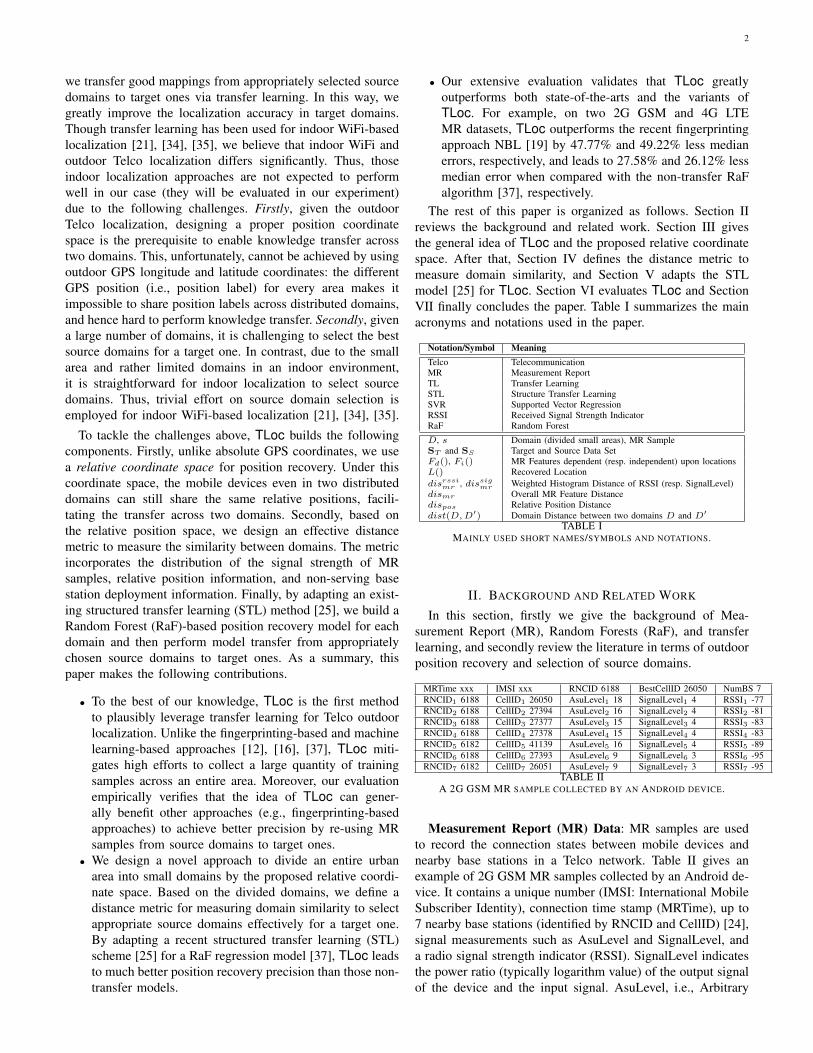


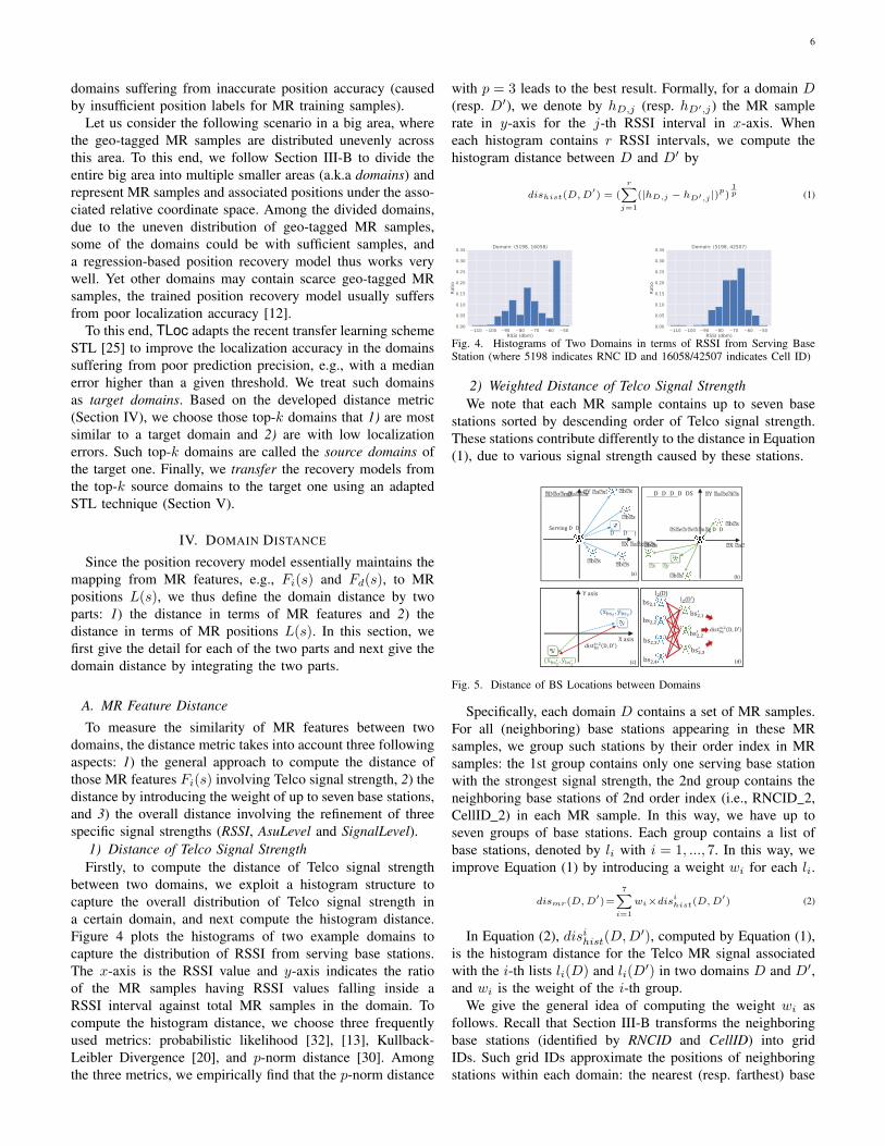


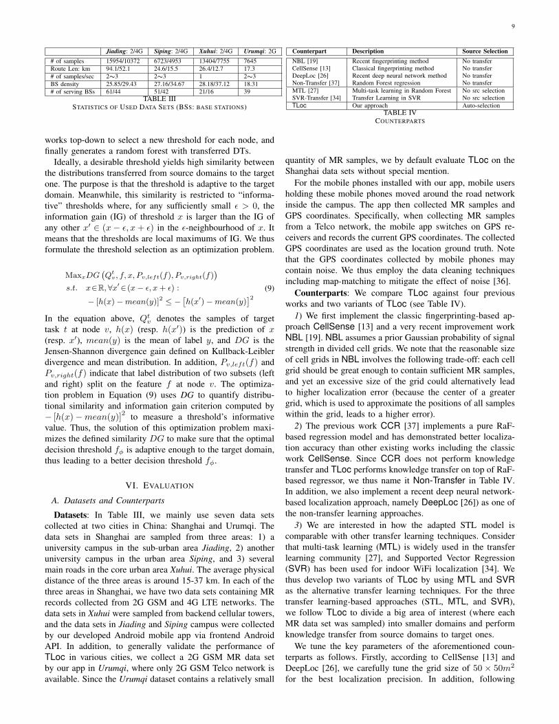
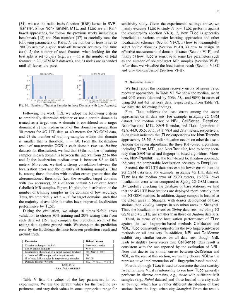
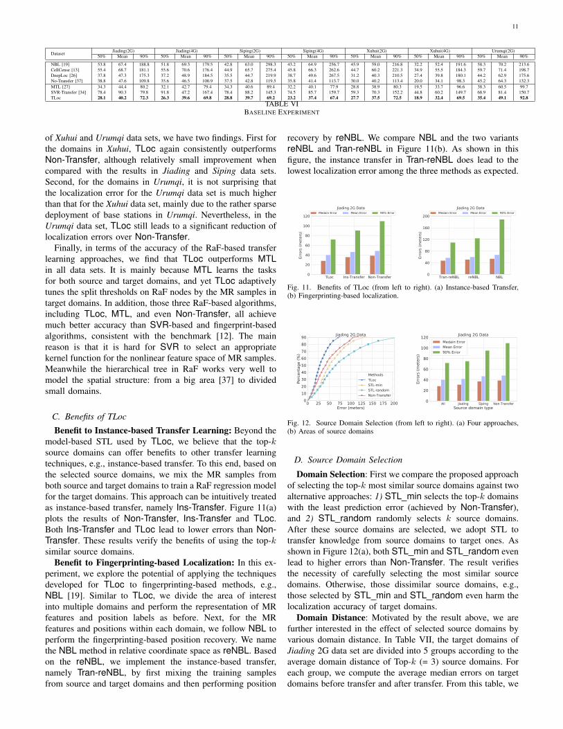


![Transfer Learning-Based Outdoor Position Recovery with ...homepage.tudelft.nl/8e79t/files/pre-print-tmc2020.pdf · Google MyLocation [2] approximates outdoor locations by the positions](https://static.documents.pub/doc/80x56/6059ea4bc0123a1a4f1f87fa/transfer-learning-based-outdoor-position-recovery-with-google-mylocation-2.jpg)


