GEOPHYSICS, VOL. 51, NO.8 (AUGUST 1986); P. 1608-1627, 24 FIGS.

Transient electromagnetic response of a three-dimensional body In a layered earth

Gregory A. Newman*, Gerald W. Hohmann*, and Walter L. Andersont

ABSTRACT by a large rectangular loop is substantial when host currents are strong near the conductor. The more con­ductive the host, the longer the galvanic responses will

The three-dimensional (3-D) electromagnetic scatter­ persist. Large galvanic responses occur if a 3-D conduc­ing problem is tirst formulated in the frequency domain tor is in contact with a conductive overburden. For a in terms of an electric field volume integral equation. thin vertical dike embedded within a conductive host, Three-dimensional responses are then Fourier trans­ the 3-D response is similar in form but differs in mag­formed with sine and cosine digital filters or with the nitude and duration from the 2-D response generated decay spectrum. The digital filter technique is applied to by two infinite line sources positioned parallel to the a sparsely sampled frequency sounding, which is re­ strike direction of the 2-D structure. placed by a cubic spline interpolating function prior to We have used the 3-D solution to study the appli­convolution with the digital filters. Typically, 20 to 40 cation of the central-loop method to structural interpre­frequencies at five to eight points per decade are re­ tation. The results suggest variations of thickness of quired for an accurate solution. A calculated transient is conductive overburden and depth to sedimentary struc­usually in error after it has decayed more than six ture beneath volcanics can be mapped with one­orders in magnitude from early to late time. The decay dimensional inversion. Successful 1-D inversions of 3-D spectrum usually req uires ten frequencies for a satisfac­ transient soundings replace a 3-D conductor by a con­tory solution. However, the solution using the decay ducting layer at a similar depth. However, other pos­spectrum appears to be less accurate than the solution sibilities include reduced thickness and resistivity of the using the digital filters, particularly after early times. (-0 host containing the body. Many different l-D Checks on the 3-D solution include reciprocity and con­ models can be fit to a transient sounding over a 3-D vergence checks in the frequency domain, and a com­ structure. Near-surface, 3-D geologic noise will not per­parison of Fourier-transformed responses with results manently contaminate a central-loop apparent resistivi­from a direct time-domain integral equation solution. ty sounding. The noise is band-limited in time and even­

The galvanic response of a 3-D conductor energized tually vanishes at late times.

INTRODUCTION tions include an asymptotic solution for a sphere in a layered host (Lee, 1981) and Fourier transformation of 3-D thin-plate

The behavior of transient electromagnetic (TEM) fields over responses using the decay spectrum (Lamontagne, 1975). a three-dimensional (3-D) earth is not yet fully understood. We introduce a technique for computing the transient re­The need for further theoretical insight is reflected by the sponses of arbitrarily shaped 3-D bodies within a layered increasing demands placed on transient electromagnetic meth­ earth. The solution is formulated in the frequency domain, ods for petroleum, mineral, and geothermal exploration (Nabi­ and results are Fourier transformed to the time domain. The ghian, 1984). Computer solutions exist for calculating the tran­ Fourier transform is carried out using sine and/or cosine digi­sient responses of 3-D thin plates in free space (Annan, 1974) tal filters developed by Anderson (19751, or using the decay and for a 3-D prism in an otherwise homogeneous half-space spectrum technique of Lamontagne (1975) and Tripp (1982). (SanFilipo and Hohmann, J985). Other 3-D transient solu- Thefrequency-domain solution is developed from an integral

Presented at the 54th Annual International Meeting, Society of Exploration Geophysicists, Atlanta. Manuscript received by the Editor August 13, 1985; revised manuscript received December 20, 1985. *Department of Geology and Geophysics, University of Utah, Salt Lake City, UT 84112-1183. tU.S. Geological Survey, Box 25046, MS 964, Denver Federal Center, Denver, CO 80225. ([; 1986Society of Exploration Geophysicists. All rights reserved.

1808

1609 TEU Response of a 3-D Body in the Earth

equation solution described by Wannamaker et al. (l984a), adapted for loop and grounded-wire source fields.

The model study presented investigates the transient elec­tromagnetic responses of a 3-D dike-like body within a lay­ered earth energized by a large rectangular loop. Also investi­gated are practical 3-D structural problems for the central­loop configuration. The types of structural problems empha­sized are detection of sediments beneath volcanics and esti­mation of the thickness of conductive overburden.

INTEGRAL EQUAnON FORMULAnON

Frequency-domain integral equation

In Figure 1 is a 3-D body in an n-layered host. The body is confined to layer j; Gb and G j are the conductivities of the body and layer l, respectively. The impedivity i = iro~ is assumed to be that of free space. Displacement currents are ignored in the formulation.

The electric field integral equations for the unknown total electric and magnetic fields are given by

E(rJ = Ep(r) + (a b - cr) I<;;(r, r')E(r') di', (1)

and

H(r) = H17(r) + (Gil - 0) Ic;r{r, r')E(r') dv', (2)

where E,.(r) and "per) are the primary electric and magnetic

»j;P;;, ~Mp ""fo,e

erl d,

a'2 d2

o "}

~

dn- 1(T n-l

CTn

FIG. 1. 3-D body in a layered host. J and M, are impressed 17

electric and magnetic sources.

fields due to impressed-loop or grounded-wire sources and one-dimensional earth layering. The tensor Green's functions G~(r, r') and G~(r, r') relate the electric and magnetic fields. respectively, in layer / to a current element at t' in layer j, including / = j. The derivations of the tensor Green's func­tions are given by Wannamaker et al. (1984a).

Equations (1) and (2) replace the 3-D body by an equivalent scattering current distribution (Harrington, 1961). This scat­tering current is defined by

J. (r) = (0" - crJE(r), (3)

where J~(r) is nonzero only over the volume of the body.

N..merical solution

At this point if the electric field in the body were known, electric and magnetic fields could be computed anywhere using equations (1) and (2). Van Bladel (1961) shows that equation (1) is also valid inside the body since a principal value of the integral exists. A matrix solution can then be constructed from equation (l) using the method of moments (cf', Harrington, 196~), with pulse basis functions and delta testing functions.

Hohmann (1975) showed that if the 3-D body in equation (1) is divided into N cells, the total electric field at the center of cell m due to ]V cells can be approximated by

N

Eb(r,•.> = Ep{rm) + L (0,.,. - (i)r.~(rm; Tn)' Eb(r,J, (4) ,,= 1

where E"(r",) is the total electric field at the center of cell m. Unlike the solution from Wannamaker et al. (1984a), E,,(r m) is the primary electric field for a finite source, not a plane-wave source. In each cell the body conductivity abo and total electric field are assumed to be constant and the tensor Green's func­tion for a prism of current is defined by

r~(rm; rn) = 1G~'(rm' r') do', (5) ".

Equation (4) can be rearranged to

t [(<T•• - <T)[;('.; '.) - iM,.l· E.(.j ~ -Ep (' . ), (6)

where

r! if m = n, and §m.n =-lQ (7)

if m # n.

The tensors! and Qare 3 x 3 identity and null tensors, respec­tively, Finally, considering all N values of m, a concise matrix equation is written as

~.Eb=-Ep, (8)

where ~ is the complex impedance matrix of order 3N. Equation (8) is solved for the total electric fields within all

the cells. Once the electric field in the body is known, the electric and magnetic fields outside the body are given by discrete versions of eq uations ( I) and (2). That is.

N

E(r) = [per) + L fa,,_ - o)[:(r; r")· E/I(rn) , (9) "=1

1610 Newman et 81.

and

N

H(r) = "I'(r) + L (crh, - (1)[~(r; r.) • Eh(r,,). (10) ~= 1

The cells representing the body need not be cubic. In many cases the numerical solution can be improved by subdividing the body into rectangular prisms rather than cubes (Wanna­maker et al., 1984a). Modifying the solution is simple. since integration of the tensor Green's function over a prism [equa­tion (5)] can be treated as a summation of integrations over cubic subcells. Rectangular cells are useful for approximating an elongate body, provided the scattering current is polarized parallel to the strike of the body. Use of elongated cells is justified because the scattering current varies more rapidly over the short direction of the body. We recommend, however, that cells be cubic near corners of an elongate body because variations in the scattering current are more abrupt there.

Designing the cell discretization of a body is based on the skin depth and depth of burial of the body and on the spatial variation of the excitation field. The variation of the excitation field is determined by the frequency and the physical size of the transmitting source. Specifically. cubic subcell sizes should be less than one skin depth. When small transmitting sources are used, cubic subcell sizes should be at most one-quarter of the skin depth of the body. Prismatic cells can have elongated dimensions of up to several body skin depths when large transmitting sources are used.

The computation time required to build and factor the im­pedance matrix can be excessive; the matrix is full, with di­mensions 3N x 3N, where N is the number of cells. Fortu­nately, Tripp and Hohmann (1984) show that the time re­quired to build and factor the impedance matrix can be sub­stantially reduced for a body with two vertical planes of sym­metry. The impedance matrix for such a body is block diago­nalized using group theory (e.g., Hall, 1967). The block-diagonalized matrix consists of four subrnatrices, each with dimension (3N/4) x (3N/4). The block-diagonalized matrix now requires one-quarter of the storage of the original matrix. and the number of operations required for matrix in­version is smaller by a factor of 12. Furthermore, the memory requirement is reduced by a factor of 16, because it is only necessary to store one of the four subrnatrices in memory at a time. The time required to formulate the matrix for a sym­metric body, including block diagonalization of the impedance matrix, is about one-third of that for a body with arbitrary shape. However, the option of calculating responses for gener­al bodies is maintained by solving equation (8) directly for a nonsymmetric body.

Since we use pulse subsectional basis functions to track the electric field inside the body, our solution will fail as the con­ductivity of the layer containing the body (5) becomes very small. As discussed by Lajoie and West (1976)and Hohmann (1983), the problem lies in the disparity between the sizes of the induction and galvanic operators, which relate to the vector and scalar potentials, respectively, for the scattered field. The induction and galvanic operators are defined by writing the tensor Green's function in equation (5) as the sum of two parts representing current and charge sources:

r: = A[; + q.rt (11)

where ...c[~ is the induction operator and Cl[~ is the galvanic

operator. The galvanic operator relates to sources of electric charge. The induction operator appears to be dominated by the galvanic operator, and it is lost when added to the galvan­ic operator in equation (11). Lajoie and West (1976) avoid the problem of the disparity of the sizes of the two operators by solving for curl-free and divergence-free scattering currents inside a thin, 3-D plate. Their formulation is in the frequency domain, and the plate is embedded in a layered half-space. Recently, SanFilipo and Hohmann (1985) used a similar ap­proach for solving for the scattering currents inside a prism within a conductive half-space. Their solution is a direct time­domain integral equation solution that is valid in the limit of free space.

Based on checks with other numerical solutions, we believe our solution will accurately calculate currents that simulate galvanic current distributions as well as currents that are simi­lar to 2-D induction current distributions. However, it will not accurately simulate responses from a 3-D induction current vortex because the galvanic operator dominates in the numeri­cal solution. In general, the solution's accuracy depends upon the frequency, the spatia] variation of the excitation field, the resistivity of the host. and the geometry of the body. For example, our solution would fail for a cube embedded in a resistive host if it were excited by a source field that varies rapidly with frequency and position. Two comparisons of the 3-D solution with other solutions for plane-wave and dipolar sources show good agreement for the plane-wave case and poor agreement for the dipolar case (Hohmann. 1983). In these comparisons, the conductivity contrast between the body and half-space host was I 000, where the plane-wave comparison was made at 300 Hz and the dipole comparison was made at I· 000·Hz. Also; the. dipolar source. field falls. off quite rapidly with position, while the plane-wave source field exhibits no geometric decay. OUf solution works best for elon­gate, low-contrast conductors in the fields of large loops and long grounded wires that vary smoothly in space where elon­gated cells can be utilized. The 3-D solution is more appropri­ate fOT the low contrast structure problem than for the prob­lem of mineral exploration in areas of high contrast. Experi­ence shows that- the- 3-D snlution works best for contrasts in conductivity between body and host of less than 300: L

Verification of results

Any valid numerical solution must satisfy reciprocity. Figure 2 shows a three-layer model where the depth of Ion· m overburden varies from 20 to 40 m. Beneath this variable overburden are two more layers of resistivity 100 and I 000 n· m. The depth to the 1 000 n· m basal half-space is 60m.

At position a (x = - 150. y = 0), we placed a loop source with surface area S = 400 m2

. At position 6 (x = 100, Y = 0), we placed a grounded-wire source with length ( = 20 m. Reci­procity states that the vertical magnetic field evaluated at a

due to the grounded wire at f, is

H~ = - E~ 1/(iU>I.1S), (12)

where E~ is the y component of electric field evaluated at t> due to the loop source at a (Harrington. 1961). Equation (12) is approximate since it is assumed that the magnetic and elec­

1611 TEM Response of a 3·D Body In the Earth

3-D BODY PLAN VIEW

Gl r-----+--l· --:

200",

Q

~

SCALEI I -+

• y o 50

3-D BODY CROSS·SECTION

10,n·", 20",

IOC n·", 60",

1000 n·m FIG. 2. Model used for reciprocity check.

tric fields do not vary over the surface area of the loop or the length of the grounded wire, respectively.

Equation (12) is used as a check by first computing directly the primary and scattered electric field E~ due to the loop source. The primary field is defined as the field due to the loop and 2-D earth; the scattered field is the field scattered by the body. The sum or primary and scattered fields is the observed total field. The vertical field H~ is then given from equation (12). Figure 3 compares the primary and scattered magnetic fields computed directly from the 3-D solution and indirectly from equation (12). The comparison shows excellent agree­ment, in both real and imaginary parts, over a frequency range from IOta 3000Hz. The computation time required for this 160-cell body is about 10 minutes per frequency on a VAX­11/780.

For another check. we can use the results for a 3-D integral

SCATtERED MAGNETIC fiELD

equation solution developed by Das and Verma (1981, 1982). Their approach differs from ours in one important way: the secondary tensor Green's functions, which are Hankel trans­forms, are evaluated directly with digital filters. The tensor Green's function is composed of primary and secondary parts. The primary part is the whole-space component and the sec­ondary part is the reflected component due to earth layering. In contrast, we evaluate the secondary tensor Green's func­tions by tabulating them with digital filters on a grid, and then interpolating the tabulated forms to any desired position (Wannamaker et at, 1984a). By tabulation and interpolation, a substantial reduction in computation time is realized. Das and Verma's solution is similar to ours in that pulse basis functions are used to track the electric field within the body. However, they use cubic rather than prismatic cells.

The two solutions are compared in Figure 4. Das and Verma published a solution for this overburden model in Das and Verma (1982). The 1 n .m body has dimensions 30 x 120 x 90 m and is embedded in a 100 (l·m basal half­space beneath overburden that is 10 m thick and has resistivi­ty of 10 Q. m. Depth of burial is 30 m, A central profile is made across the body with a horizontal loop-loop system where separation of the transmitting and receiving loops is 150 m. The scattered vertical magnetic field is plotted in Figure 4 as a percentage of the free-space vertical magnetic field.

Even though the shapes of the 3-D anomalies in Figure 4 are similar. agreement between the two solutions is not good because of the different numbers of cells representing the body. Das and Verma use 12 cells while we used 12, 96, and 768 cells. Using 12 cells to track the electric field within the body is inadequate for our solution. As the number of cells increases to 96 and 768, our solution is converging. The smallest size cdr we use is 7:5 m, one-hall' the skill depth- of the- body. Because we have used small transmitting sources (l m x 1 m square loops), the cell size should be at most 3.75 m, one­quarter of the skin depth of the body. We could not discretize the body with this cell size because of prohibitive computation time. Das and Verma use a cell size of 30 m, two skin depths in the body, but this size is inadequate for tracking the electric field within the body. Additional checks on our numerical

PRIMARY MAGNETIC FI ELD j10-5 )10-'

Re (Hz) . \ __._!~~~~~Li I -·-l

\ --,

"­ 1 I \ -, I I -,lOT

/'(°'1 J I \0, 1m (Hz)

1

'" 1m ""I~)

I, " / I '/

-,j ..

"­10. 7 f- '\ 1)0-6

-,

"

L ; I

103 102 103 102 10

f (Hz) f (Hz)

FIG. 3. Reciprocity check. The solid dots are calculated using equation (I2) and the curves directly from our 3-D solution.

1612 Newman et al.

solution {or a plane-wave source are given in Wannamaker et al, (f984a):

CO~PUTATION OF TRANSIENT RESPONSES

T.e decay spectrum

The Fourier transformation of a 3-D frequency-domain re­sponse could in principle be calculated using a fast Fourier transform (FFT) algorithm. However, the number of fre­quencies required for an FIT is very large, and simple inter­polation over a sparsely sampled freq uency response does not give accurate results (cf', Lamontagne, 1975; Hohmann, 1983). We are interested in calculating transient responses from a sparse set of frequency-domain values defined over a suf­ficiently wide band. A sparse set of frequency data is necessary because each 30-0- computation requires- a long time for corn­putation. Several workable techniques exist for transforming a

frequency

in-phase

:'::'""-" ".\'\ \\ :~

'II ~:

-1~

I'~-

-5

;1: '. J E ~l II :" ·f -10h\ j,[ ~\ i~ '1' ". ~, \ i ,! ~I \ / It -15 .1 , I:;l . : /: ~\ \ ..' I! ~\ \ I,t ~ t "......... . I: ;\ 1= : \ ,::\ I: : \ I : ': \ I : : \ / : ~ \,~/ ;. .

.....

sparsely sampled frequency-domain response to the time domain. One, such technique uses the decay spectrum of La­montagne (1975) and Tripp (19HZ).

The frequency-domain system function H(ro) and the time­domain impulse response h(t) for an EM field component are related by the Fourier transform pair

and

H(ro) = LOT)h(t)e-ilJ)t dt, (13)

I(t) = -l J~ H(CJJleilJ)t dill, (l4)27t - oo

where it is assumed that the impulse response is causal [i.e., h(t) = 0, t < 01

The impulse response can also be written in terms of the

= 1 000 Hz

quadrature

120 0_

'.~ . "1': ....).\._//

\. .I'

1/: '(,i r: F f. f

o /:

'I J: : J:

1,..-

-120

" •.:.:.;.,;j

Newman et.al. solutions /1 cells _ .. _ .. ­

96 ceJJs - -- ­768 ce1ls ....... "'"

~150m----1

! ~

(m) +­

120

with

10.n om

100.n 'mT 90m

Pb = 1n'm1 j.....lIj

30m body strike length: 120m

FIG. 4. Comparison with results of Das and Verma [1981, 1982).

1813 TEM R••pons. of • 3-D Body In the Earth

Im(H.) ~I>I

-"Tt"(~l

In ",..21 10'" 1000r>; I,om",. "oi,,'

.\ /r·-',.,

i '\ i.SpOT". somp/.li DI IP Jr.ou.,,~iu./ "

100,10·' " '\

-, -,

\ 10"

10'0 ""-, -,",

MOOEl -, "­___;=-=-~~~ __L _1 -,

/ / /' . -."i,. " "i,,,. j '"~ -, 10- 7 -,

C"l~ -, ~~ IO/J-", ".Io-to.,--lT 0.1

,ooy STRitE • IO~",

10000 1 000 100 10

f,.qu.nC;y {H~}

FIG. 5. Horizontal magnetic field response sampled at 19 fre­quencies.

. ~ dl

("VI",')

100 000 f­

};"r;.r l

trol'l,lor",.tl " .."on,.,"'-.\:,/' ~rOlf'! loop of '(Imp

\

Iro", ~otto"., of u:".p"....)\. \10000 '. ~

\:\. \\

'\ \1

1000 f­ \-\ ~~I ~, \;.

100 !­ \~ II"\\ ~I

l 10 f-

... \'t, ~ 1\

\,I I I 001 0.\ \0

Ii'''' { ... l

FIG. 7. A comparison of soundings for the total vertical mag­netic field component.

tii,eel _ /1'0'" lop of ""tip

~~~;:f:;~;<.~. .\ _/'ouri., "~""o,,,,.rI "'fUM"

/./'....:-;, I,ottl bolto'" 01 'DIII,/ " ..

/I\i ~::~ j I ).1\ : : '".c • I .' : I 1,

.~

~

~ \~

:1\MOCH

\:.F~Z~7-=~- \ G~l IOn·"

-"~-Ir .oar st rue » lOa'"

\

\ 0_01 0.1 10

tim. 1.. 01

FIG. 6. Comparison with results from a direct time-domain integral equation solution-horizontal magnetic field.

inducing electric '(eld

fran,,,,iftrr //~ ~

vortex current

~. 't'~ indUCing Jme varying m09ntfi~ field

golvonic r/JrrMf

FIG, 8. Galvanic and vortex currents induced by a conducting 3-D body. Figure taken in part from McNeill (1985).

-----

1614 Newman et al.

1.0

ohz at [-!.. )

mot

0.1

O.Ot

0.001

3-D 2-D

",-- --,-lms I r ms

~ -> -, .>: 2\Ct\ 0-- ­-\ /-"1ms

3•• __ \ ~ '_" T_S' - -7 -- 1- ~~- t - _~

5ms ......... \ f===~~~~------ 9m$

~.) L_ .... __ ",tl f~--

15ms__ :=::~ I '-.j~"'~ = "" .. - - - - ... - ;;; ~ ~ - Conductor ~:-V '::' --...-.:­

Position ----r----; 1- -- ­r---t---Conduc'or

Posit ion 25ms-'-'­II - - - '~.-;::L -' ­

35ms....... I '-. ­....................... j ,;

I MODFI

r---500m--+JOO"'1 I 40 ....

z;;, w$ ~-l--""" ID·m

(u".nr' 'OA IO()[}·m I

0.000 II I I , I I I ! I I I I ! I ! I I , I I

-90 -70 -50 -3V -10 10 30 50 10 90 -90 -10 -50 -30 -10 \0 30 50 10 90

dl,tance from center of conductor (III) dlshnt' frOIl\ c&nhr of conductor 1m)

FIG. 9. Comparison of 3-D and 2-D vertical magnetic field responses for a conductor in a half-space. Light lines show half-space responses. Loop and conductor 600 m long in the 3-D case.

decay spectrum A(k) where

vertical field decoy 61 I • -30m

h{t) = Lao A(k)e- if dk. (15)

The impulse response is estimated from sparse frequency­domain data by treating equation (13) as an inverse problem for h(t). We solve equation (13), a Fredholm integral equation of the first kind, by the method of moments (Harrington, 1968), using exponential basis functions and the delta testing c3n z functions. We approximate h(t) from equation (15) by at

N

h{t) = L Alle- k n l , (16) (m:s

AJ

.01 n=1

where k. is the nth decay constant. Substituting equation (16) into equation (13) and incorporating delta testing functions gives

N An = H(ro ). 001 mL k +ilfl",

(17) ,,- 1 n

Writing equation (17) for each of the M values of m gives a matrix equation:

15'A = H, (18) .0001 .1 10

from which to determine the N values of An' The impulse t (ms)

response is then given by equation (16), and the response of FIG. 10. 3-D and 2-D decay curves of total vertical field at

any transmitter waveform can be calculated by convolution. x = -30. At late times the 3-D and 2-D total fields decay as The solution of equation (18) is described in detail in Tripp the half-space fields at t - 5J2 and t - 2, respectively.

100

--

--10 3-D

O.5m,-==:C)h l ~ ~

--.....A )

--'""­

( ....

7 - ...... , 3m, '-- __ '" \ I

0.1 ~ - ~ ~ ---~ ­,Sm6,/\\ -1-' - ~

--~-~t ,---_- -" \ ,--- \, '/ ' 9ms _ r.. r '- _-.l\ J -- .........

0.01 - - - - '.' I ~'

---- .... 'I' I15m, - __ '"~,I__ , _ _ __ ",

--;o:~u--;;;,. I 'I, I Position ~II . ........1­0.001 ._'-- ,'-,-­25m.=:= -~'~'_'I'_

35m. .................... :....,..\:.: ..:::.f- ...

0.000 I ' """. , ... ,I

-90 -70 -50 -30 -10 10 30 50 70 90

dlstonct froll! center of conduc tor (m)

FIG. It. Comparison of 3-D and 2-D vertical field responses;

2-D O.5"u~ -::::::::­

~"""'--

lmJ~ ~__~~~:~ "" --- -­-4 m !: 2J

/" ~ ­ •3"'S.:~ .. __ " \ / i

; ~

5ms~ )': .,,/- -~ - ~\~ - '- ­ a <, /-­ I»

to) ---- ... ~ \ \ / . ...­9ms- - - - -- ,-\_ -, _ T- _ o --- \ ".J ' m

8­0<-----:':-:-...---\ 't::! ....... _-­'------,15ms __ --- i"', _ :i g III/\1 , _ m-_._~~.---.~. __ .­ II25m, '- . -, - Con due 10' ~

~Po$ilion35lit,· , t " , , .,. ,. ••••••• ", " ••• ~ • ~ ~ ~ ~ ~ t, ••

MODEL

I--'00. ----+--Joo...:t=: .0• -.,-.-- '~~ :-- ­~ 'L w" .

IOQ-m lO.m C"".nt =IO~ loo,O.m

I , , , , , I, ' " ,

-90 -10 -~O -30 -10 10 3Q 50 10 90

~lstllllC' fu .. cute, of cplldlle:tor (III)

conductor in contact with 40 m thick. 10 Q. m overburden.

.... en.... C.h

-- -- - -------- ---

10 I

3-D 2..0",-, / <,

O.5ms'\: 1.0 /" ....................

~ /\ y"

o.s «, cHI

,)I'cH 3ms~ 4/~7 ........A ) (m:s

0.1

/"1'(\ I " , 5ms ~ ....

/ - -.::..:--~--/

;I' .... - - - - ;;;--- --;. - - - - - ­0.01 ;I' ...--f............ Contluclor ,...- .. ' ~ ... -

Posilion _... -­9ms _~ _ 15ms-----~-- ,

~ConrJucfor/" .... _ Posi/ion

;I' .... .-" ......... _._­;I' "

/ " -- - ~_.--25m~'-- . -- ­15ms0.001 - .-.""",

./ ''-.

es»,- ",

--'­0.000 I ' I" I I I I , , , I I , I , I I I I I ,

-90 -10 -50 -30 -10 10 30 50 10 90 -90 -10 -50 -30 -10 \0 30 50 10 90

di'hnce fro .. center Df con~uchr (III) distanc. froll enter of conductor (.)

FIG. 12. Comparison of 3-D and 2-D horizontal field responses; conductor in contact with 40 m thick. 10 Q. m overburden.

C"".""IOA

Wire

~...•OJ

I

•zE :I•~

~

!!

1617 TEM Response of •

(1982). Since equation (18) is ill-posed, a generalized inverse solution is required with N greater than M. Usually ten fre­quencies are sufficient. However, a fair amount of subjectivity is involved in choosing the best of all possible solutions pro­vided by a generalized inverse solution. Furthermore, the 3-D transient calculated in this way is also unstable at late times.

Sine and cosine transformation 'Via convolution

Popular digital filtering techniques offer an alternative ap­proach for calculating 3-D transient responses. The Fourier transformation of a 3-D frequency response for a causal step turnoff can be calculated using a sine or cosine transform, where

ah(t) = ~ f:>:'Im [H(ro)J sin (roc) di», (19)at 1t Jo and

2 I,r 1m [H(Ol)]h(t) = - - cos (rot) dss, (20)

rt 0 (t)

The quantity 1m [H(oo)] is the imaginary part of an EM field component. The transient and its time derivative are given by h(t) and ah{t)!Vl. The quantity t7h(t)/c7c is equivalent to the impulse response h(t} in equation (14). For completeness, the integral transforms in equations (19) and (20) can also be ex­pressed by

(Jh(f) 21"­-:1- = - - Re [H(ro)] cos (rol) de: (21)

(.( 1t 0

'- vertical fl,ld "', decay at x • -30m \\

\ , with If) n'm overburden \ \, \

\ \3-D I

, 2-D~hz I I

ll~ch I ,{ \ t : 3-DA )(irH' \~\

2-D-.

OJ

.001

10 100

t(msl

FIG. 13. 3-D and 2-D decay curves of total vertical field at x = -30.

3·D Body in the Earth

and

. 2 IOC) Re [H(ro)] . h(t) = h(O) - - sm (rot) di». (22)

n 0 (t)

The quantity Re [H(ro)] is the real part of an EM field compo­nent and 11(0) is the initial value of the field component at zero time. We have obtained better results evaluating the above integral transforms by using the 3-D imaginary field- compo­nent lm (H(co)]. Thus, from a computational standpoint, we prefer using equations (19) and (20) instead of equations (21) and (22). Numerical evaluation of these sine-cosine transforms is carried out with Anderson's (1975) digital filters.

Johansen and Sorensen (1979) note that the Fourier sine­cosine transforms can be expressed as special cases of half­order Hankel transforms, specifically,

t: sin li22 f(x) (21tsx) dx = r I"" 'All).,}} 1: 1/2 (Ar) dA, (23) o cm 0I

where (' = (21t)1!2, r = sc, A. = xc, and fl(A) = j(Ajc)/i.}!2. This implies that the filter design method using Hankel transforms for integer or real orders in Anderson (1975, 1979, 1982a) can be followed to design Fourier sine-cosine filters by way of linear convolution theory.

The digital filters are designed by casting equations (19), (20), (21), and (22) into the general form

f(b) = r"; F(g) sin (bg) dg. (24)Jo cos

If we let x = In (b), y = In (1/g) and multiply by £7"', equation (24) becomes

fa:· [ X- Y sin y)]eX.f(eX) = . F(e- Y) e (ex - dy. (25) _y, cos

Equation (25) is now in the form of a linear convolution inte­gral with F(e Y) and eXf(eX) as the input-output function pairs. From the convolution theorem, the filter response may be determined from known input-output function pairs. Accord­ing to Anderson (1975), the choice of these function pairs is critical for the design of good general purpose filters. Filter accuracy is improved significantly, and the length and mag­nitude of the filter tails are reduced by selecting known convo­lution integrals having rapidly decreasing input and output function pairs. Furthermore, using such input-output function pairs results in filter weights that accurately evaluate a wide class of sine-cosine transforms. The best input-output function pairs found by Anderson (1975) are

l' 9 exp (_a2g2) sin (gb) dg = ..Ji~ b exp (_b 2/4a2)/4a3, (26)

and

2I' exp (_a 2 g ) cos (gb) dg = v;; exp (-b 2/4a2)/2a, (27)

where a > 0 and b > O. The integral transforms in equations (26) and (27) are from Gradshteyn and Ryzhik (1980).

By Fourier transform theory, convolution in equation (25) is equivalent to multiplication in the transform domain, where we write

I(i) = F(.i) §(.i). (28)

--------

10 ,

3-D 2-D 1m,

/~

~ /' " <,1.0 O.5m~ .......

<. / <, cth. <, <,c)f

<, ( ,.~, ) /~

0.1 r 3m$ 3mz" <,

~-~ 5ms ;' ..... ­5ms-- - ­-- - - - ~

------------=== \.-- -: - "'-..... ,/ ,

~ms ' - - - -- /'

....... -""'" .... ",.---.. ;;;: ~ =::: - ­0.01

ISms ~ - - .... -- --­--.-------------- ­~m$ - - - - - - - - - ~_Conductor

.",.,., . _ . Position---------=:::== --. --.­25ms~' -­..--..---Conductor --;' ­

0001 Position 35m, .: ....................•.........•..... ~ ... :::.

0.000 1 I I' I I I I , I I ! !. I I I I ! , I I I I

-90 -10 -50 -30 -10 to 30 50 10 90 -90 -10 -50 -30 -10 10 30 ~O 10 90

distance from center of conductor (ml dlstonce from center of con4uctor (Ill

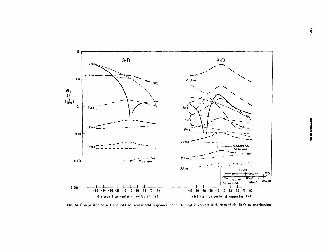
FIG. 14. Comparison of 3-D and 2-0 horizontal field responses; conductor not in contact with 20 m thick, 10 n· m overburden.

.... !Z ClD

I

z CD

~ II :3

!. ~

1619 TEM Response of a 3-D Body in the Earth

PLAN VIEW

1:-------------.., I ,-----------, I I I I I I I I I I I t I # .,-J,a/ionI I I I ,,# '1,# ?,#I I 1 I o 0 0 c';"< .. It I I t.f:F -c[ I I , '.) '\ e-: I I I , I I r I I J

I I I I I_~-_=_.=__=_: .=_==:~J

y

CROSS-SECTION o

10n·m SOOm

100 n·m \ I 1000 2000m

SCALE

FIG. 15. Structure model of an overburden layer with variable thickness,

~-'-.J...~~ =',,",

\0" ~\\. \10 "

\ '\ '\ \

\\'\ ICY'

starron 500 '\ stalion 1 000 \ 10- 1 '0'.-· i-- ..- J-e· \--- -. 1-0 \

sltiltiOn 1 DOOstation 5001:)"' Ic,'1 f I._.~ ~-~ "- -'-- J /:?-- -"'"

I .::.::;:.:/10' ~---~~;;;.? 10'· \ j

- '-- 1-D\ i

\ ..----. I·)

10' -,o°f---------- ----t. I

1~1':S

I ",() .~

.. o station 1 500 station 2 000 station 1 500 ~lfttion 2000e.

1:)"' \, ~:;:/;;; 1------__.>:d ;(Y

0..0'0-' 10·>1 ~ l_~

10-' inlJ 'c,21 "

'0" station 2 5CO station :1SOO

10 ~?/ f--.----------.-~/

station 2 500 10

---l I.\..;.... 101 1~1i it)) 10' l~i leO 10' 10'

tlfte(nu) tirfle (R1,)

FIG. 16. Transient decay plots for the vertical magnetic field FIG. 17. Apparent resistivity soundings at stations 500, 1 000, at stations 500, 1 000, 1 500, 2 000, 2 500, and 3 500. When I 500, 2000, 2 500, and 3 500. Tht: soundings are truncated solid and dashed curves coincide, the body is not detectable. after 400 InS because of numerical noise.

1820 Newman et al,

PLAN VIEW

rJF~

a=lOSS-SECTION

-­rn·",10u

1 OOOU.m

--­ 1 8OOm-­ ~

1 600n

--­ -2700m­ 2000m

iiQU.m

FIG. IS. Simulation of sedimentary structure beneath vol­canics. MT and central-loop stations [for loops 2 x 2 km) are located at x = 500.1 000,2 500, and 3 000.

500 t 000

1000 l-D response__~/O'O - • • . ~/ 1-Drespollse /' .;,..

oD6erwd

<,.\!>-: " .

100 I-D response oorr(lSpond",g to ~truClu,..n;gh

~ I------c--­ 3:=~~-j2500~ I

1 000 . __ 1-0 '"PMse ._---~,'>~ l·D response

obssMK1.;...::...:><,.~> J

/"_.100

1-0 rellfXHlt/IJ e«respofldmg l-D responl8 corresPonding to ~ruC11.J1'fI 11;9" 10 slruetlJ~ nigh

10 100 10 100

t {l'II~)

FIG. 19. Central-loop apparent resistivity soundings.

The transformed functions in equation (28) form the following transformed pairs:

l(i) +-+e"!(x), FCi) +-+F(x).

The transformed filter response is then given by

§(i) = tvvF(x), (29)

provided both input and output function pairs have band­limited Fourier transforms. This restriction is required since sli)--. 0 for _i- ± tx .

The final steps in designing the digital filters follow from Koefoed et al. (1972), Anderson (1973, 1975, 1979, 1982a), and Verma (1977). The input-output functions in equations (26) and (27) are cast in the form or equation (25), and each input­output function pair is digitized from small to large abscissa values. A constant sampling interval of Ax = .20 is selected to yield single-precision accuracy (i.e., relative errors $ 10- 6). The discrete Fourier transform is applied to the sampled input-output functions, and the spectrum of the filter response is obtained from equation (29). Division by zero in equation (29)is avoided by selecting a suitable initial sampling point.

Next, tile spectrum of the filter response is multiplied by the Fourier transform of the sine function

sine (x) = sin (1tx/L\x)!(ltxjL\x), (30)

and the result is inverse Fourier transformed to obtain the filter sine response or filter weights. The convolution integral in equation (25) is then approximated by a discrete convolu­tion sum, and the integral transform in equation (24) is evalu­ated as

f{b) = LKI JtiF[cxp (Ai - X)]}Ib, (31)

where H'i arc the filter weights for the sine or cosine transform and Ai - x are the shifted abscissa values. Note that x = In (b). The limits N 1 and N:2 on the summation can vary between 1 and 266 for the sine filter weights and between 1 and 281 for the cosine filter weights. The actual values N 2 and N 1 are determined by adaptive convolution (Anderson, 1982a, 1984), which depends upon how quickly the product Jot; F[exp (A 1 - x)J damps out for filter weights corresponding to large and small abscissa values. If the product does not damp out sufficiently to a specified truncation tolerance, then equation (31) will yield nonconvergent answers. However, if F(g) is a continuous bounded function, then convergence will occur due to the rapid decrease in the amplitudes of the filter tails. Accel­erated convergence will also occur if IF(g) 1- 0 as g ....... ± 00.

As Anderson (1975, 1982a, 1984) pointed out, equation (31) works best for kernels that are not highly oscillatory. In cases with highly oscillatory kernels, other numerical integration methods are suggested (cf., Boris and Oran, 1974). Fortu­nately, the digital filtering technique works well for the 3-D EM kernel since we are solving a diffusion equation (displace­ment currents are neglected). The EM kernels are absolutely decreasing functions and are not highly oscillatory.

Calculating 3-D transients with digital filters is a straight­forward extension of a procedure commonly employed for calculating I-D and 2-D transients (cf., Anderson 1973, 1981, 1982b; Kauahikaua and Anderson, 1977; Tsubota and Wait, 1980). We first compute a suitable frequency sounding using our 3-D solution. The sine or cosine transform is evaluated

1621 TEM Response of a 3-D Body In the Earth

j 10 700 10 100 1000

I (Hz)

FIG. 20. MT apparent resistivity soundings Pyx for a primary electric field polarized in the y direction.

500

7000 I-D f9sponse " .................::-;:.--::::=--~...:::'"

"v'/ ~ ,

OO"rwdy::~::/ ...._ ­__,,</ .....--- 7·0 response ~rrespOrnJing

700 ~?.:-.;-,,::~.:_:-~o-- - /0 Slruc1u,., high

E c ~ 2500

1000

"D~>_ --'-<, ,

obsBl\'8d'..: ~ ..

)·D r9sponfe correspondIng100 rostructure high

1000 I

/-- jzz:»:">....,--­""" <:::'/ ""- J·D r&ponss correspondIng

_-":,;--,,,,:-c:~ -> -- 10 strucru~ ItIgh

3000

I.D-rsspotlSll... ------- --'-_"'_,

->- / '''---ObsefWC,~ _ .' / -------.....,

, ,~: 1-0 rBSfXJflss corresponding

/0 structure high

using a fast digital filtering technique described as lagged convolution by Anderson (1982a, 1984). We apply the digital filtering technique to the discretized frequency function, which is replaced by a cubic spline interpolating function. If the bandwidth of the frequency response is sufficiently wide, then points outside the bandwidth can be truncated or replaced by known asymptotic values during the convolution. The sine and cosine lagged convolution is rapidly computed for any time range and interval by using another spline interpolation, whose sampling interval is identical in time to the digital filter spacing. The power of the lagged convolution method over conventional convolution is realized by computing and saving all function values for the first time point, thus saving many recomputations for all remaining times.

The integral transforms in equations (19) and (2[») usually require 20 to 40 direct 3-D frequency evaluations at five to eight points per decade. Al very high frequencies, the response at the earth's surface of a deeply buried body is usually small compared to the response of a layered earth. Thus evaluating equations (19) and (20) may not require calculation of the 3-D response in the high-frequency band. The layered-earth re­sponse can be substituted for the 3-D response when the scat­tered field is four or five orders of magnitude smaller than the layered-earth field. The highest frequency we use to evaluate equations (19) and (20) corresponds to a source-receiver and/or body-receiver separation of approximately five skin depths; the body is also considered to be an EM source. Any 1-0 or 3-D response requiring a frequency greater than this cutoff frequency is set to zero for integral transform evalu­ation. The truncation may destroy the accuracy of the very early-stage transient, but since these early times are never cal­culated, the truncation error is considered negligible.

When low-frequency 3-D responses are required for evalu­ating the sine and cosine transforms, we truncate the kernel in the sine transform and use the asymptotic form

1m [H(<o)J = Ki» (32)

for the kernel of the cosine transform. This low-frequency

asymptotic expression is for the imaginary part of a 3-D EM field component and is valid in the near field when the 3-D response is dominantly galvanic. The constant K is real and depends upon the impressed source, the earth layering, and the body geometry and electrical properties; K is determined from the low-frequency behavior of the 3-D results. We could also use the asymptotic form in equation (32) for the sine transform. However, in that case whether the kernel is trunca­ted or is represented by equation (32), the calculated transient (lh(t)/(:1, is the same.

The accuracy of evaluating sine and cosine transforms with digital filters is dependent upon the digital filter coefficients, the lagged convolution truncation tolerance, and the accuracy and sampling of the 3-D frequency response. The accuracy of the final transient is primarily dependent upon the accuracy of the original 3-D frequency response. Typically, we seek about three-figure accuracy for intermediate times in the transient and five-figure accuracy in the corresponding frequency re­sponse.

Empirically, we found errors in the calculated transient after it decays about six orders in magnitude from early to late time. DOUble-precision filter weights exist (Anderson, 1983), but we consider them impractical because the frequency re­sponse must also be computed in double precision. The 3-D solution in its present form cannot be improved using double­precision arithmetic. Thus the accuracy of the late-stage tran­sient will always be questionable because the 3-D frequency response has limited accuracy. Furthermore, we found that the low-frequency asymptotic form in equation (32) makes no contribution to the late-stage transient (Kaufman and Keller, 1983).

Checks on Fourier transformation

Obtaining independent checks on our 3-D Fourier transfor­mation techniques is difficult. Fortunately, the 3·0 direct time-domain integral equation solution of SanFilipo and Hohmann (1985) provides such a check.

1622 Newman et al,

Figure 5 shows a check on our digital filtering technique in which the transient response of a .5 Q. m body embedded in a 10 {}. m half-space is calculated. The body dimensions in cross-section are 40 m in width and 30 m in depth extent. The body strike extent and depth of burial are 100 and 30 rn, respectively. A 100 x 100 m square loop is centered 50 m from a position directly over the center of the body. The frequency responses in the vertical and horizontal magnetic fields (Hz and H.J are sampled at 19 frequencies at the loop center. The imaginary component of H;x is plotted in Figure 5 from 10000 to 1 Hz. Since we are calculating the horizontal field, the field we calculate is the scattered field. The discretized frequency function is replaced by a cubic spline and Fourier-transformed

500 I 000

PalOm)

100 10e.n'm

con,,"

10 100 I 000

TIME (m~l

2500 I 000

Pa(SJ,·ml

100 r- 686.1'l.", lnlo,p,ot.d Mod.1 60"-~

1,82 SJ, .., I !109m

52 n·... I

~ 10010

TI ME (ms 1

FIG. 21. 1-0 least-squares fits for central-loop apparent resis­tivity sounding curves. The 1-0 fits are for three layers at stations 500. 1 000, and 2 500.

using a sine transform [equation (19)]. Figure 6 shows the Fourier-transformed horizontal voltage decay from .1 to 10 InS for a step-current turnoff where the calculated voltage is

2for a receiving coil of 1 m area. Our Fourier-transformed response is compared with San­

Filipo and Hohmann's (1985) solution. Their solution is for a linear ramp turnolT in current; measurement times are referred to both the top and bottom of a .05 ms ramp between .5 and 2.5ms and a .25 ms ramp after 2.5 ms (Figure 6). For compu­tational efficiency, the length of the ramp is changed from SanFiJipo and Hohmann's (1985) solution at later times. Notice that the Fourier-transformed response typically falls between the measurements made at the top and bottom of the ramp. It can be shown that, to a first-order approximation, the average of the two ramp responses is that of a step-current turnotT. After lO ms, there is numerical noise in the Fourier­transformed response and the check with SanFilipo and Hoh­mann's solution is not very good. We also show a check on the vertical voltage transient in Figure 7; again the agreement is excellent. It is encouraging to obtain such good agreement between the two 3-D solutions, because they are formulated in different domains and use different matrix formulations. The direct time-domain solution uses the Galerkin method for forming the matrix, while the frequency-domain solution uses the point-matching method with delta testing functions. The two matrix formulations are also dependent upon the cell design- of the 3-D body; the frequency-domain solution. allows for variable cell dimensions while the direct time-domain solu­tion does not.

A check on the decay-spectrum technique and our 3-D solu­tion was shown in Sanf'ilipo and Hohmann (1985). This check once again showed excellent agreement. We now present 3-D transient responses calculated with the decay spectrum and with digital filters. However, we currently favor calculating 3-D transients with the digital filtering technique rather than with the decay spectrum, which is harder to use. The compu­tation time required for both Fourier-transformation tech­niques is insignificant-a few seconds for digital filtering and a minute or two for the decay spectrum on a VAX-ll/780. These computation times do not include the time required to calculate the 3-D frequency sounding, which is the most time­consuming step in the calculation ofa 3-D transient response.

GALVANIC RESPONSES

Consider the 3-D conductive body in Figure 8. When this body is in freespace and is in a time-varying magnetic field, vortex currents are generated within the body. From Fara­day's Jaw, these currents flow in a direction such that the change in magnetic flux linking the body is minimized. The EM response of the body is called an inductive, or vortex current, response. The vortex current response vanishes when the inducing magnetic field is no longer time-varying.

Now consider thc body in Figure 8 embedded in ground of Ilnite conductivity. If an inducing electric field is present, cur­rent will flow within the ground that will be concentrated near and at the conducting body since the body is more conductive: than the ground. The name commonly given to this EM field behavior is "current channeling" or "current gathering." However, we prefer the term" galvanic response," since cur­rent is deflected away from a resistive body. The galvanic response is caused by boundary polarization charge at resis­

1623 TEM Response of a 3·D Body In the Earth

La y ered Earth Host

1001I·m-- 50m

1 OOO.o,·m

2000m

50.Q.·m

2 500 89fi·m--60m

1182Sl'm

1869m i2_0EO~!- _

52,n'm

1000 l06il·m--49m

903fi'm

(1 550 ml

1 766m

60,n'm

500 lOaD:·m 42m

815,n'm

Ll_4Q°.!!lL -- ­

17~m

62 n'm FIG. 22. Three-layer interpretation shows a volcanic unit whose resistivity changes laterally. A small rise in basement is detected. The dashed lines show the correct depth to basement. The layered-earth host far from the basement high is shown for comparison.

tivity discontinuities. The polarization charge is required to satisfy the boundary condition that the normal component of current density be continuous. The galvanic response will exist whether the inducing electric field is time-varying or not. In general, the EM response of a 3-D body within a layered half-space is a complex interaction of both vortex and galvan­ic responses. In some cases, however, the EM response of a 3-D body can be dominated by either the vortex or the gal­varuc response.

COMPARISON WITH 2-D RESPONSES

There are important differences between transient responses of elongate 3·D conductors energized by a large rectangular loop, and 2-D structures of identical cross-section energized by two infinite line sources. These differences are important because until recently only 2-D modeling programs were available for general models.

figure 9 compares, for a step-current shutoff, the 3-D and 2-0 vertical magnetic field responses for a dike. The dike is a {n· m body embedded in a roo (1. m half-space. Its depth extent is 60 m, its width is 20 m, and, in the 3-D case, its strike length is 600 rn. The dike is buried at a depth of 40 m. We energized the dike with a large loop, 500 x 600 m in the x and y directions. The 2-D responses were computed using the finite-difference time stepping program of Adhidjaja et al, (1985). Instead of a loop, the 2-D responses were generated by two finite line sources parallel to the strike direction of the 2-D structure. Therefore boundary charges are absent in the 2-D formulatoin. If the 2·0 dike were energized with a rec­tangular loop, there would bc galvanic effects in the 2-D re­sponse. Therefore we suspect that the 3-D and 2-D responses would compare more closely if a 2-D response had been gen­erated with a rectangular loop rather than with two infinite line sources. The value in comparing 3-D responses generated by a rectangular loop to 2-D responses generated by two infinite line sources is to show some of the limitations of 2-D modeling.

In Figure 9, the 3-D and 2-D responses are similar in form but they differ in magnitude and duration. The difference in the source field falloff with time for the 3-D and 2-D models is reflected in the total field falloffs. For a loop, the late-time

2falloff of j}h~/at is t- 5/ , while for two infinite line sources, the

falloff is t 2. Thus 3-D responses can differ from 2-D re­sponses by an order of magnitude. The 3-D anomaly in this example is virtually all due to galvanic sources, since the scat­tered field falls off as an inverse power at late times rather than as an exponential (SanFilipo and Hohmann, 1985). The 2-D anomaly, on the other hand, is due purely to induction. Figure 10 shows the decay in 3-D and 2-D total fields at station x = - 30.

Figures 11 and 12 illustrate vertical and horizontal mag­netic field responses, respectively, for a model where the dike of the previous case touches conductive overburden. We expect galvanic effects are present in the 3-D responses: cur­rent is pulled down from the overburden into the body. How­ever, there can be no vertical current distortion in the 2-D responses. This is confirmed in Figures 11 and 12 where, unlike the case in Figure 9, the 3-D anomaly is larger than the 2-D anomaly. In Figure 13. decay curves for 3-D and 2-D total vertical field responses are plotted at x = - 30.

Figure 14 illustrates the response of the 3-D body when it is detached from the conductive overburden. Its response is weakened because current in the overburden is not channeled into the body (compare Figures 12 and 14).

Differences in the falloff with time of Jayered half-space fields for infinite line and finite loop sources show up in the falloff of the 2-D and 3-D scattered fields. At the window in time when the half-space field is weak compared to the scat­tered field, the 3-D and 2-D anomalies have similar forms, but they can differ by an order of magnitude. Galvanic effects are not present in 2-D responses; hence the 2-D responses are due purely to induction currents. On the other hand, galvanic ef­fects in 3-D responses can be very large. SanFilipo et al. (1985) shows that galvanic effects are important when half-space cur­rents are strong in the vicinity of a 3-D structure. We find

1624

I

Newman et at.

that, if the layered host is sufficiently conductive and in con­tact with the 3-D conductor, strong current in the background medium will persist to later times and galvanic effects will last longer.

APPLICATIONS TO STRUCTURE PROBLEMS

Overburden thickheSS

OUf solution can be applied to modeling geologic structure. Consider the problem of mapping the thickness of conductive overburden. Figure 15 illustrates a 3-D, variable-thickness

500

ooo

overburden model with layer resistivities of 10 and 100 n·m. Directly over the basement depression the overburden layer thickens to 1 100m, while far away from the depression, the layer thins to 500 m. In plan view the basement depression extends 2 800 m in the x any y directions. Six central-loop stations, with loops 1 krn on a side, profile over the basement depression at x = 500, 1 000, 1 500, 2 000, 2 500, and 3 500 m.

Figures 16 and 17 are plots of the transient decay of the vertical magnetic field and the apparent resistivity sounding defined by the decay of the magnetic field time derivative chz/ot. Again these responses are for a step-current shutoff. The apparent resistivity sounding is obtained by inverting the central-loop half-space formula,

oh. pl1t3

/2

[ . ].--.::.. Z = -3- 3 erf (r) - (3z + 2z3

) erf' (z) u(t), (33)at 1:.

for resistivity p. In equation (33), L = fi ao where ao is the equivalent radius of the square loop and erf (z) is the error function. The value z is defined as L/2[~/(p7tt)J 1/2 and u(t) is the unit step function. The inversion of equation (33) is evalu­ated using an algorithm described by Raab and Frischknecht (1983).

When a central-loop station approaches the basement de­pression, the split in the 3-D and 1-0 responses (magnetic and apparent resistivity) occurs earlier, as shown in Figures 16 and 17. We define the 1-0 response as the response of the layered earth without the depression. The effect of the basement de­pression is to increase the magnetic field and lower the appar­ent resistivity relative to the 1-0 response. The 3-0 magnetic field and apparent resistivity responses are reflected by the slow decay of currents in the earth. The 3-D magnetic field anomaly and apparent resistivity anomaly are band-limited in time. Eventually, with increasing time, the transient response of the 3-D structure must vanish and approach the I-D re­sponse. At station 500, the apparent resistivity sounding in Figure 17 reflects a sampling of 10 a· m material later in time (and hence depth) than the 1-D response. Indeed, by using Anderson's (1982c) I-D TEM inversion program for the central-loop configuration, we obtained 700 m depth to re­sistive basement at station 500 compared to the actual depth of I 100 m. This depth estimate is by no means accurate. However, it points out that the conductive overburden is thickest over station 500, as would be expected since station 500 is over the basement depression.

Sedimentary structure beneath volcanics

An important structural problem for the petroleum industry is to estimate the depth to conductive sediments beneath vol­canic cover. Figure 18 shows a simulated section for such a case, The top layer consists of 100 n· m material, 50 m thick, representing thin alluvial fill. Below this layer a 1 000 n· m basalt layer of variable thickness covers a 50 n· m sedi­mentary basement. The depth to the conductive basement varies, and the problem is to determine whether central-loop transient electromagnetic methods can map these variations. The basalt cover has a maximum thickness of 1 950 m and thins to 1 350 m directly over the basement high. The base­ment high extends 3 000 m in the strike direction.

We calculated central-loop apparent resistivity soundings for loops 2 km on a side on a profile across the center of the

1625 TEM Response of 8 3·D Body In the Earth

model at positions 500, 1 ()()(l, 2 500, and 3 000, as shown in Figure 19. Compare the transient soundings with the mag­netotelluric (MT) soundings shown in Figure 20. The MT soundings are calculated for an electric field polarized parallel to strike using the algorithm described by Wannamaker et al. (1984a). Once again, the I-D responses are defined as layered­earth responses without the body. The I-D response corre­sponding to the structural high is for a conductive basement raised to I 400 m depth.

The 3-D transient soundings in Figure 20 show a rise in apparent resistivity from 100 n· m before I ms to about 700 to 850 n· m by 5 ms. At late times the soundings approach 50 Q·ro, the resistivity of the basal half-space. The largest 3-D responses occur at stations 500 and I 000. directly over the structure. As expected, the response of the body is band­limited in time and falls between the two layered-earth re­sponses.

The MT response of the body in Figure 20 is obvious in stations 500 and I 000. However, the MT response of the body is not band-limited in frequency, but is present to arbi­trarily low frequencies. This permanent distortion of the ap­parent resistivity sounding curve with falling frequency is an electric field anomaly caused by a boundary polarization charge at resistivity boundaries (Wannamaker et at, 1984b).

Comparison of the central-loop method and MT method points out a fundamental ditTerence between them. In the MT method, the plane-wave source field is always on; hence the 3-D distortion in the apparent resistivity sounding will be present to arbitrarily low frequencies. With transient methods, the transmitting source is turned off, and currents perturbed by a 3-D body must decay and dilTuse away with increasing time. Unlike the MY case, near-surface 3-D geologic noise does not permanently distort a central-loop apparent resistivi­ty sounding; geologic noise is band-limited in time, The ad­vantage of the MT method, however, is that great depth of exploration can be achieved. provided the data are interpreted properly.

I-D inversion is the standard technique used for estimating

the depth to conductive sediments. We used Anderson's (l982e) 1-0 transient electromagnetic inversion program for the central-loop configuration and set about inverting the 3-D soundings in Figure 19 to 1-D geoelectric sections. The ob­served data from 1 to 500 ms were inverted to three- and four-layer models.

The three-layer interpretation in Figures 21 and 22 shows a thinning and reduction in the thickness and resistivity of the volcanic unit over the basement high. The volcanic unit has a resistivity of 815 Q. rn at station 500, but at station 2 500 the resistivity increases to 1 182 n· m. The interpretation also shows that the minimum depth to conductive basement is I 760 m at station 500, whereas the correct depth to basement is 1 4OOm.

A constrained four-layer interpretation in Figures 23 and 24 appears to estimate the depth to a conductive zone beneath the volcanic Gover more accurately than with three layers (compare Figures 22 and 24). Moreover, the constrained three­layer interpretation and the unconstrained four-layer interpre­tation will not give layered-earth models that match the true basement depth as well as that given in Figure 24. A con­strained four-layer interpretation in which the volcanic unit is held fixed can replace the basement high in Figure 18 by an equivalent conducting layer which has variable resistivity and thickness at a similar depth. The interpretation in Figure 24 shows this layer to have resistivities of 144, 199, and 41 U' m and depths of } 497, 1 540, and J 948 m at stations 500, 1 000, and 2 500, respectively. However, the above estimates of this equivalent layer can vary significantly. Moreover in practice many field surveys will not have control of the resistivity of the overburden; hence, use of a constrained four-layer inter­pretation is often impractical with real data.

CONCLUDING REMARKS

Accurate 3-D transient responses can be generated ef­ficiently and effectively with digital filters or with the decay

La yered Earth Host

lOO.o.-m--50m

2 500

lOO.Q·m--50m

1000 100.Q·m--50m

500 100.Q·m--50m

1 OOO'u·m 1 000 ,n'm

IOOO,u'm looon'm

2000m 1948m (2000mfln- ---­

-"'2221m

1540m [1550ml

199,Q-m1869m

'1400..,)-------1497'"

144n-m

2027m

SO ,n'm 53.o.-m 56fi-m 55,u-m

FIG. 24. Four-layer interpretation shows a thinning in the volcanic unit as sounding stations approach the basement high. Note that the volcanic unit is constrained at 1 000 n·m in the interpretation.

1626 Newman at al.

spectrum. With digital filters, we found 20 to 40 frequencies at five to eight points per decade were typically required for an accurate solution. Usually we found the calculated transient

was in error after it had decayed six orders in magnitude from

early to late time. The error was present because 3-D fre­quency responses were computed with limited accuracy. Cal­culating 3-D transient responses with the decay spectrum re­quired fewer frequencies than with digital filtering (usually ten frequencies). However, transients calculated with the decay spectrum appeared to be less accurate than those calculated with digital filtering, particularly at later times. We now favor

use of digital filters for both accuracy and simplicity. The 3-D frequency-domain solution described uses pulse

basis functions to track the electric field within the body. While these basis functions produce good results when 3-D

responses are dominantly galvanic. they do not work well for high-contrast models where both induction and galvanic sources determine the EM response. We believe divergence­free basis functions must be added before high-contrast models can be correctly calculated. The solution is reliable up to a conductivity contrast between body and host of 200 : 1.

Future work should include an exhaustive investigation of 3-0 bias on 1-0 transient inversions. The need for such a

study is imperative since t-O interpretations are now being applied routinely (and perhaps incorrectly) to 3-D geologic environments. Other important practical problems that need

investigation are the transient response of a grounded wire

over a 3-D earth and the transient response of a polarizable 3-D body for both loop and grounded-wire sources. The tech­niques we used to calculate transient responses for loop sources are valid for grounded-wire sources as well. Finally, more work is required on evaluating the advantages and dis­

advantages of various EM methods in both the frequency domain and time domain. Calculating 3-D transient responses

can provide some additional insight into design of optimal field surveys.

The 3-D transient responses presented here were calculated on a VAX-l 1(780 (with a floating point accelerator but with­out an array processor) and UNIVAC] 161 computers. The computation times for both computers are approximately the same. The maximum computation time of any model present­ed was about] 2 hours. most of which was consumed in calcu­lating the 3-D frequency response.

ACKNOWLEDGMENTS

Discussions with Phil Wannamaker were essential for devel­oping the 3-D frequency-domain solution, and Bill SanFilipo provided important insight on the behavior of 3-D transient

responses. We further acknowledge Perry Eaton, who provid­ed the direct time-domain integral equation results. We are

also indebted to Frank Frischknecht. U.S. Geological Survey, Denver, who made the VAX-l 1/780 computer available for part of this study.

Financial support was provided by the following corpora­tions: Amoco Production Co.: ARea Oil and Gas Co.; Chevron Resources Co.; Conoco Inc.; CRA Exploration Pty. Ltd.: Sohio Petroleum Co.; Union Oil Co. of California; and

Utah International Inc. Additional funding was provided by

the U.S. Army Research Office under contract DAAG29-83­K-OOI2.

REFERENCES

Adhidjaja, J. I.. Hohmann, G. W., and Oristaglio, M. 1.. 1985. Two­dimensional transient electromagnetic responses: Geophysics. SO, 2849-2861.

Anderson. W. L., 1973. Fortran IV programs for the determination of the transient tangential electric field and vertical magnetic field about a vertical magnetic dipole for an m.layered stratified earth by numerical integration and digital linear filtering: Nat. Tech. Inf. Servo rep. PB-221-240.

--- 1975, Improved digital filters foc evaluating Fourier and Hankel transform integrals: Nat. Tech. Inf. Servo rep. PB-242-800.

---- 1979, Computer Program: Numerical integration of related Hankel transforms of orders 0 and 1 by adaptive digital filtering: Geophysics, 44, J287-1305.

1981, Calculation of transient soundings for a central induc­tion loop system (Program TCILOOP): U.S. Geol. Surv. open-file rep. 81-1309.

- 1982a, Fast Hankel transforms using related and lagged convolutions: Assn. Compo Math., Trans., Math. Software, 8, 344­368.

1982b, Calculation of transient soundings for a coincident loop system (Program TCOLOOP): U.s. Geol. Surv. open-file rep. 82-371:L

--- 1982c. Nonlinear least squares inversion of transient sound­ings for a central induction loop system (Program NLSTCI): U.S. Geo!. Surv. open-file rep. 82-1129.

1983, Fourier cosine and sine transforms using lagged convo­lutions in double-precision (subprograms DLAGFO/DLA/GF1): u.s. Geol. Surv. open-file rep. 83-320.

--- 19R4, Computation of Green's tensor integrals for three­dimensional electromagnetic problems using fast Hankel trans­forms: Geophysics, 49, 1754 1759.

Annan, A. P., 1974,The equivalent source method for electromagnetic scattering analysis and its geophysical applications: Ph.D. thesis, Memorial Univ. of Newfoundland.

Boris, J. P., and Oran, E. S., 1974, Numerical evaluation of oscillatory integrals with specific application to the modified Bessel function: Nat. Tech. Inf. Serv. rep. AD/A-00219712WC.

Das, U. C. and Verma, S. K.. 1981, Numerical considerations on computing the EM response of three-dimensional inhomogeneities in a layered earth: Geophys. J. Roy. Astr. Soc., 66, 733-740.

--- 19R2, Electromagnetic response of an arbitrarily shaped three­dimensional conductor in a lavered earth-numerical results: Geo­phys, J. Roy. Astr. Soc., 68. 5~6.

Gradshteyn, I. S.. and Ryzhik, 1. M., 1980, Tables of integrals, series and products, 2: McGraw-Hill Book Co.

Hall. G. G., 1967, Applied group theory: American Elsevier Publ, Co. Inc.

Harrington, R. F.. 1961, Time harmonic electromagnetic fields: McGraw-Hili Electrical and Electronic Engineering Series, McGraw-Hill Book Co.

-- 1968, Field computation by moment methods: The Mae­\1illan Publ. Co.

Hohmann, G. W., 1975, Three-dimensional induced polarization and electromagnetic modeling: Geophysics, 40,309--324. --~ 1983. Three-dimensional EM modeling: Geophys. Surv., 6,

27- 53. Johansen, H. K., and Sorensen, K., t979, Fast Hankel transforms:

Geophys, Prosp., 27, 876--901. Kauahikaua, J.• and Anderson, W. L., 1977. Calculation of standard

transient and frequency sounding curves for a horizontal wire source of arbitrary length: Nat. Tech. Inf. Serv, rep. PB-274-119.

Kaufman, A. A. and Keller, G. V., 1983, Frequency and transient soundings: Elsevier Science Pub!. Co.

Koefoed, 0., Ghosh, D. P., and Polman, G. J., 1972,Computation of type curves for electromagnetic depth sounding with a horizontal transmitting coil by means of a digital linear filter: Geophys. Prosp., 20, 4Ofr.420.

Lajoie, J. J., and West. G. F., 1976, The electromagnetic response of a conductive inhomogeneity in a layered earth: Geophysics, 41, 1133-1156.

Lamontagne. Y., 1975. Applications of wideband time-domain elec­tromagnetic measurements in mineral exploration: Ph.D. thesis, Univof Toronto,

Lee, T. 1.. 19B 1. Transient electromagnetic response of a sphere in a layered medium: PAGEOPH. 119, 309-338.

McNeill, J. D.. 1985. The galvanic current component in electro­magnetic surveys: Geonics Ltd. Tech. Note TN 17.

1627 TEM Response of a 3-D Body In the Earth

Nabighian, M. N.• 1984. Forward and Introduction to Special Issue of GEOPHYSICS on time-domain electromagnetic methods of ex­ploration: Geophysics, 49, 849-853.

Raab, P. V., and Frischknecht, F. C, 1983, Desktop computer pro­cessing of coincident and central loop time-domain electromagnetic data: U.S. Geol. Surv, open-file rep. 83-240.

SanFijipo, W. A., Eaton. P. A., and Hohmann, G. W., 1985, The effect of a conductive half-space on the transient electromagnetic re­sponse of a three-dimensional body: Geophysics, SO, 1144-1162.

SanFilipo, W. A., Eaton, P. A., and Hohmann. G. W., 1985, Integral equation solution for the transient electromagnetic response of a three-dimensional body in a conductive half-space: Geophysics, 50. i9R-809.

Tripp, A. C, 1982, Multi-dimensional electromagnetic modeling: Ph.D. thesis. Univ. of Utah.

Tripp. A. C, and Hohmann, G. W.o 1984, Block diagonalization of

the electromagnetic impedance matrix of a symmetric buried body using group theory: Inst. of Eleetr, and Electron. Eng., Trans, Geo­science and Remote Sensing, G£.22, 62-69.

Tsubota, K., and Wait, J. R., 1980, The frequency and time-domain responsesof a buried axial conductor: Geophysics, 45, 941-951.

Van Bladel, J., 1961, Some remarks on Green's dyadic for infinite space: Trans, on Antennas and Propagation, 9, 563-566.

Verma, R. K., 1977, Delectability by electromagnetic sounding sys­terns: lost. Electr, and Electron. Eng., Trans., Geosci. Electr., GE-IS,232-251.

Wannamaker, P. E., Hohmann, G. W... and SanFilipo, W. A., 1984a, Electromagnetic modeling of three-dimensional bodies in layered earths using integral equations: Geophysics. 49,60-17.

Wannamaker, P. E., Hohmann, G. W.• and Ward, S. H., 1984h, Mag­netotelluric responses of three-dimensional bodies in layered earths: Geophysics, 49, 1517-1533.