Page 1
University of Kentucky University of Kentucky
UKnowledge UKnowledge
University of Kentucky Master's Theses Graduate School
2010
TRANSITIONAL FLOW PREDICTION OF A COMPRESSOR AIRFOIL TRANSITIONAL FLOW PREDICTION OF A COMPRESSOR AIRFOIL
Vivek Hariharan University of Kentucky, [email protected]
Right click to open a feedback form in a new tab to let us know how this document benefits you. Right click to open a feedback form in a new tab to let us know how this document benefits you.
Recommended Citation Recommended Citation Hariharan, Vivek, "TRANSITIONAL FLOW PREDICTION OF A COMPRESSOR AIRFOIL" (2010). University of Kentucky Master's Theses. 44. https://uknowledge.uky.edu/gradschool_theses/44
This Thesis is brought to you for free and open access by the Graduate School at UKnowledge. It has been accepted for inclusion in University of Kentucky Master's Theses by an authorized administrator of UKnowledge. For more information, please contact [email protected] .
Page 2
University of KentuckyUKnowledge
University of Kentucky Master's Theses Graduate School
2010
TRANSITIONAL FLOW PREDICTION OF ACOMPRESSOR AIRFOILVivek HariharanUniversity of Kentucky, [email protected]
This Thesis is brought to you for free and open access by the Graduate School at UKnowledge. It has been accepted for inclusion in University ofKentucky Master's Theses by an authorized administrator of UKnowledge. For more information, please contact [email protected] .
Recommended CitationHariharan, Vivek, "TRANSITIONAL FLOW PREDICTION OF A COMPRESSOR AIRFOIL" (2010). University of KentuckyMaster's Theses. Paper 44.http://uknowledge.uky.edu/gradschool_theses/44
Page 3
ABSTRACT OF THESIS
TRANSITIONAL FLOW PREDICTION
OF A COMPRESSOR AIRFOIL
The steady flow aerodynamics of a cascade of compressor airfoils is computed
using a two-dimensional thin layer Navier-Stokes flow solver. The Dhawan and
Narasimha transition model and Mayle‟s transition length model were implemented in
this flow solver so that transition from laminar to turbulent flow could be included in the
computations. A method to speed up the convergence of the fully turbulent calculations
has been introduced. In addition, the effect of turbulence production formulations and
including streamline curvature correction in the Spalart-Allmaras turbulence model on the
transition calculations is studied. These transitional calculations are correlated with the
low and high incidence angle experimental data from the NASA-GRC Transonic Flutter
Cascade. Including the transitional flow showed a trendwise improvement in the
correlation of the computational predictions with the pressure distribution experimental
data at the high incidence angle condition where a large separation bubble existed in the
leading edge region of the suction surface.
KEYWORDS: CFD, Turbomachinery, Flow Separation, Transition from Laminar to
Turbulent Flow, Intermittency.
Vivek Hariharan
22nd
June, 2010
Page 4
TRANSITIONAL FLOW PREDICTION
OF A COMPRESSOR AIRFOIL
By
Vivek Hariharan
Dr. Vincent R. Capece
Director of Thesis
Dr. James M. McDonough
Director of Graduate Studies
22nd
June, 2010
Page 5
RULES FOR THE USE OF THESES
Unpublished theses submitted for the Master‟s degree and deposited in the University of
Kentucky Library are as a rule open for inspection, but are to be used only with due
regard to the rights of the authors. Bibliographical references may be noted, but
quotations or summaries of parts may be published only with the permission of the
author, and with the usual scholarly acknowledgments.
Extensive copying or publication of the thesis in whole or in part also requires the
consent of the Dean of the Graduate School of the University of Kentucky.
A library that borrows this thesis for use by its patrons is expected to secure the signature
of each user.
Name Date
________________________________________________________________________
________________________________________________________________________
________________________________________________________________________
________________________________________________________________________
________________________________________________________________________
________________________________________________________________________
________________________________________________________________________
________________________________________________________________________
________________________________________________________________________
________________________________________________________________________
Page 6
THESIS
Vivek Hariharan
The Graduate School
University of Kentucky
2010
Page 7
TRANSITIONAL FLOW PREDICTION
OF A COMPRESSOR AIRFOIL
________________________________________
THESIS
________________________________________
A thesis submitted in partial fulfillment of the
requirements for the degree of Master of Science in
Mechanical Engineering in the College of Engineering
at the University of Kentucky
By
Vivek Hariharan
Lexington, Kentucky
Director: Dr. Vincent R. Capece, Associate Professor of Mechanical Engineering
Paducah, Kentucky
2010
Copyright © Vivek Hariharan 2010
Page 8
This work is dedicated to my Amma (Mother) and Appa (Father) from whom I‟ve learnt
a lot about life and who taught me to be patient and work hard to stand on my own feet.
This work will always remind me of the strength and courage they‟ve imparted to me.
Page 9
iii
ACKNOWLEDGEMENTS
I would like to take this opportunity to express my gratitude towards my advisor
Dr. Vincent R. Capece for his time and support in carrying out this research project. This
thesis could not have been made possible without his tremendous help and valuable
comments.
In addition, I would like to thank Dr. Kozo Saito and Dr. Tingwen Wu for serving
as members of my defense committee. I would also like to thank all my teachers for their
support and guidance.
I would like to gratefully acknowledge the support of Qian Zhang of our research
group in helping me in the initial phase to start with this research project and also for his
support from time to time.
I would like to thank all my family members, especially Susheela Chitti, Usha
Chitti, Murali Chitappa and Brinda Akka for their continued support, and without whom
this Master‟s degree could not have been pursued. I would like to express my sincere
gratitude towards them for having faith and confidence in me as I began my journey as a
graduate student.
I also would like to thank my friends in India and Lexington, KY for their
encouragement and support during my Master‟s work. Firstly, I would like to express my
sincere gratefulness towards my close friends Seshadri and Sripathi for their ever-lasting
moral support, kindness and words of wisdom. I would also like to thank Viji for having
been on my side, for her encouraging words, for having had complete faith and trust in
me, and for her care and support in times of need. I would also like to thank Anusha for
Page 10
iv
her support in my times of need. I would also like to thank Spandana for her encouraging
words while I was writing my thesis. I would also like to thank Dharmendra and Jhon for
their support and care during my thesis writing stage. I would also like to thank Tathagata
and Devi for having been with me and being supportive until the beginning of my thesis
writing stage. I would also like to extend my thankfulness towards Ms. Verronda for her
kindness, care and support. In the end, I would like to express my sincere thanks to
Gurdish for being extremely helpful and supportive, and for having given me company
during my thesis writing stage. Though, this thesis has been the result of my hard work
and dedication, it could not have been made possible without the support of all my
friends.
Finally, I would like to express my deepest love and gratitude towards my parents,
who inspired and instilled in me the confidence and courage to succeed in life. This thesis
could not have been possible without their blessings. They both have been a tremendous
source of knowledge and a source of strength in every dimension of life I have seen.
Page 11
v
TABLE OF CONTENTS
Acknowledgements............................................................................................................ iii
List of Tables.................................................................................................................... viii
List of Figures.................................................................................................................... ix
List of Symbols................................................................................................................ xvi
List of Files....................................................................................................................... xxi
Chapter One: Introduction................................................................................................... 1
Background.................................................................................................................... 1
Literature Review.......................................................................................................... 4
Objectives...................................................................................................................... 6
Chapter Two: Geometry and Grid Generation.................................................................... 8
Cascade Geometry......................................................................................................... 8
Airfoil Geometry........................................................................................................... 9
Grid Generation........................................................................................................... 10
Different Types of Grids........................................................................................ 11
Traditional H-grids and Sheared H-grids........................................................ 13
C-grids............................................................................................................. 15
O-grids............................................................................................................. 16
Grids for Flat Plate Studies................................................................................... 17
Grids for NASA-PW Airfoil................................................................................. 18
Chapter Three: Turbulence and Transition Models........................................................... 21
Turbulence................................................................................................................... 21
Baldwin-Lomax Algebraic Turbulence Model..................................................... 21
Spalart-Allmaras One-Equation Turbulence Model.............................................. 24
Boundary and Initial Conditions for the Spalart-Allmaras Turbulence Model..... 28
Inlet Turbulent Viscosity and Initial Condition.................................................... 29
Streamline Curvature Correction........................................................................... 30
Page 12
vi
Transition from Laminar to Turbulent Flow............................................................... 31
Mayle Transition Length Model........................................................................... 31
Dhawan and Narasimha Transition Model............................................................ 33
Chapter Four: Computational Model and Data-Theory Correlation................................. 35
NPHASE..................................................................................................................... 35
Interaction of Transition Model with Flow Solver...................................................... 36
Data-Theory Correlation............................................................................................. 37
Flat Plate................................................................................................................ 38
NASA-PW Airfoil................................................................................................. 41
Computational Procedures.......................................................................................... 41
Chapter Five: Results........................................................................................................ 42
Flat Plate..................................................................................................................... 42
Laminar Flow........................................................................................................ 43
Turbulent Flow...................................................................................................... 47
Inlet Turbulent Viscosity and Initial Condition Study.................................... 52
Production Term Formulation Study in the Spalart-Allmaras Model............. 54
Streamline Curvature Correction Study.......................................................... 57
Transition............................................................................................................... 60
NASA-PW................................................................................................................... 64
Low Incidence Angle Condition........................................................................... 65
Fully Turbulent Flow....................................................................................... 65
Baldwin-Lomax and Spalart-Allmaras Model.......................................... 69
Inlet Turbulent Viscosity Study................................................................ 73
Streamline Curvature Correction Study.................................................... 76
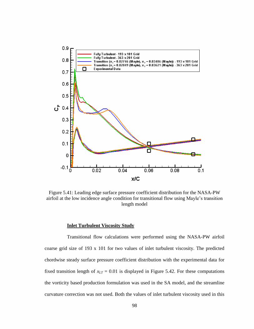
Transition......................................................................................................... 81
Inlet Turbulent Viscosity Study................................................................ 98
High Incidence Angle Condition......................................................................... 105
Fully Turbulent Flow..................................................................................... 105
Baldwin-Lomax and Spalart-Allmaras Model........................................ 110
Inlet Turbulent Viscosity Study.............................................................. 114
Production Term Formulation Study in the Spalart-Allmaras Model..... 117
Streamline Curvature Correction Study.................................................. 120
Page 13
vii
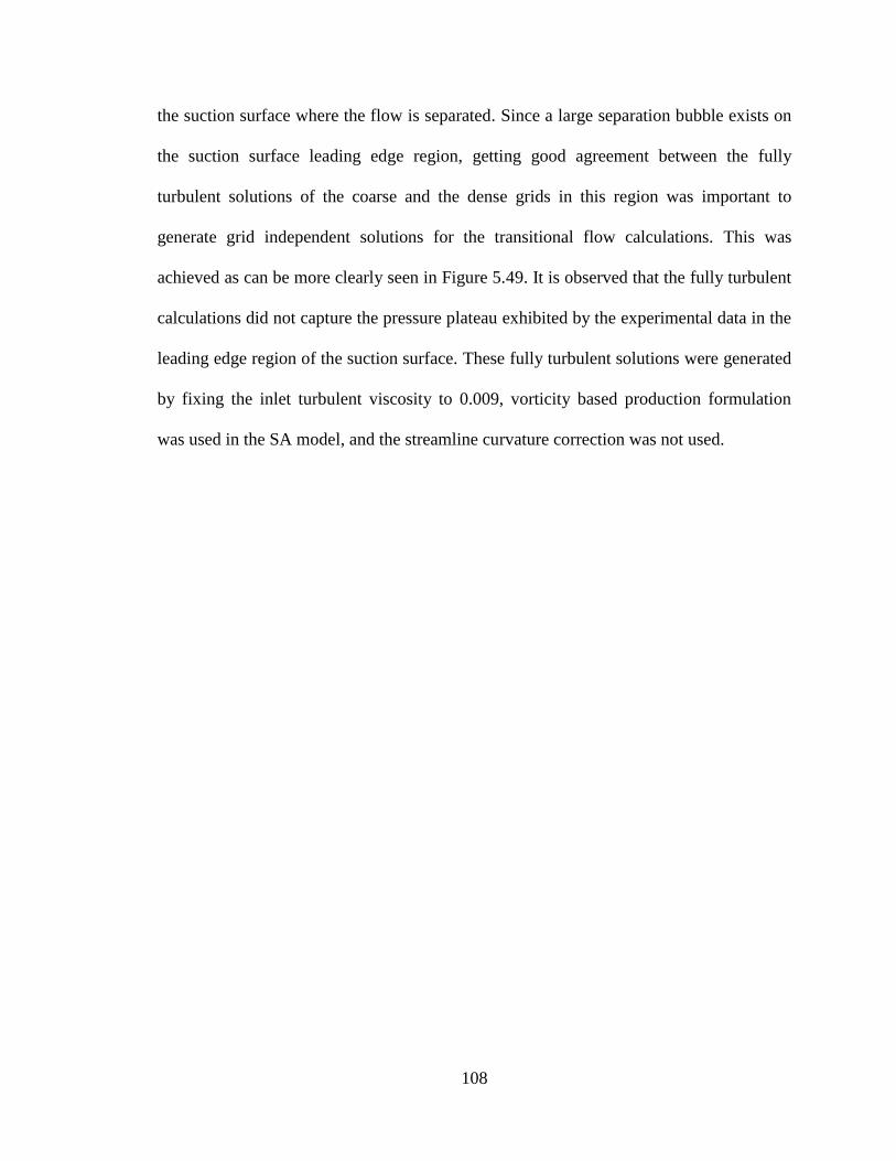
Transition....................................................................................................... 123
Inlet Turbulent Viscosity Study............................................................... 133
Production Term Formulation Study in the Spalart-Allmaras Model..... 136
Streamline Curvature Correction Study.................................................. 140
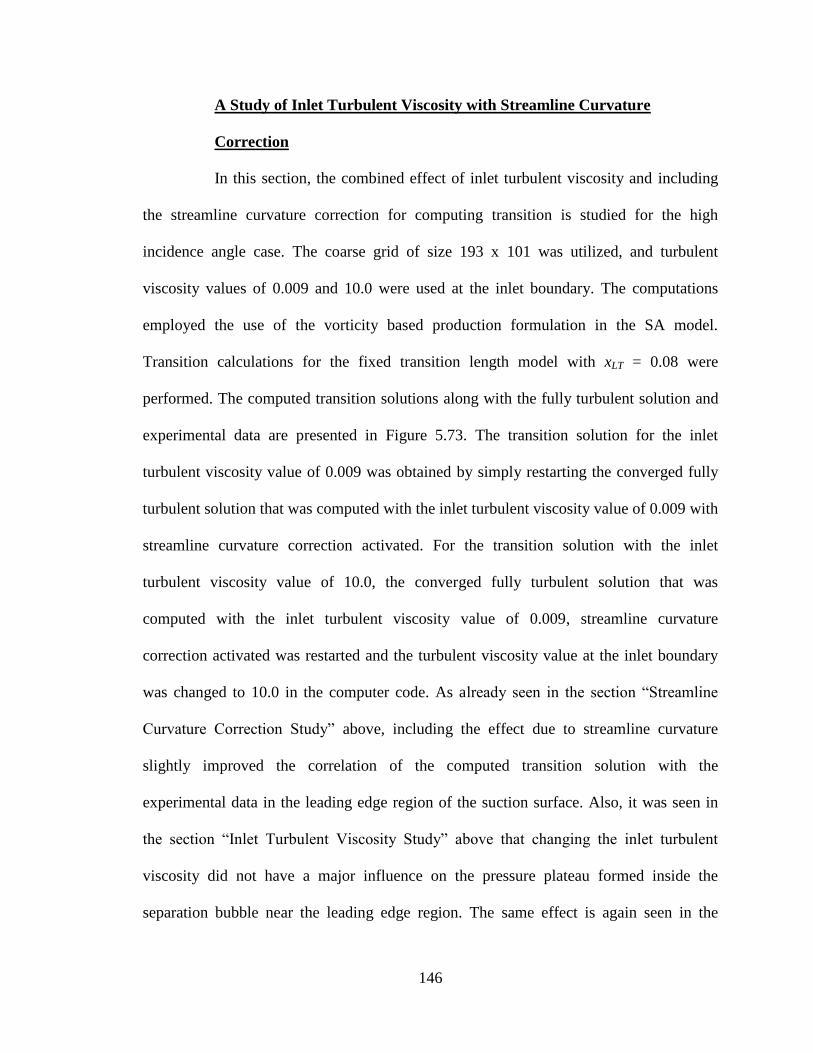
A Study of Inlet Turbulent Viscosity with Streamline Curvature
Correction.......................................................................................... 146
Chapter Six: Summary and Conclusions......................................................................... 151
Summary.................................................................................................................... 151
Conclusions................................................................................................................ 152
Future Work............................................................................................................... 157
Appendices
Appendix A: Turbulent Flat Plate Experimental Data.............................................. 158
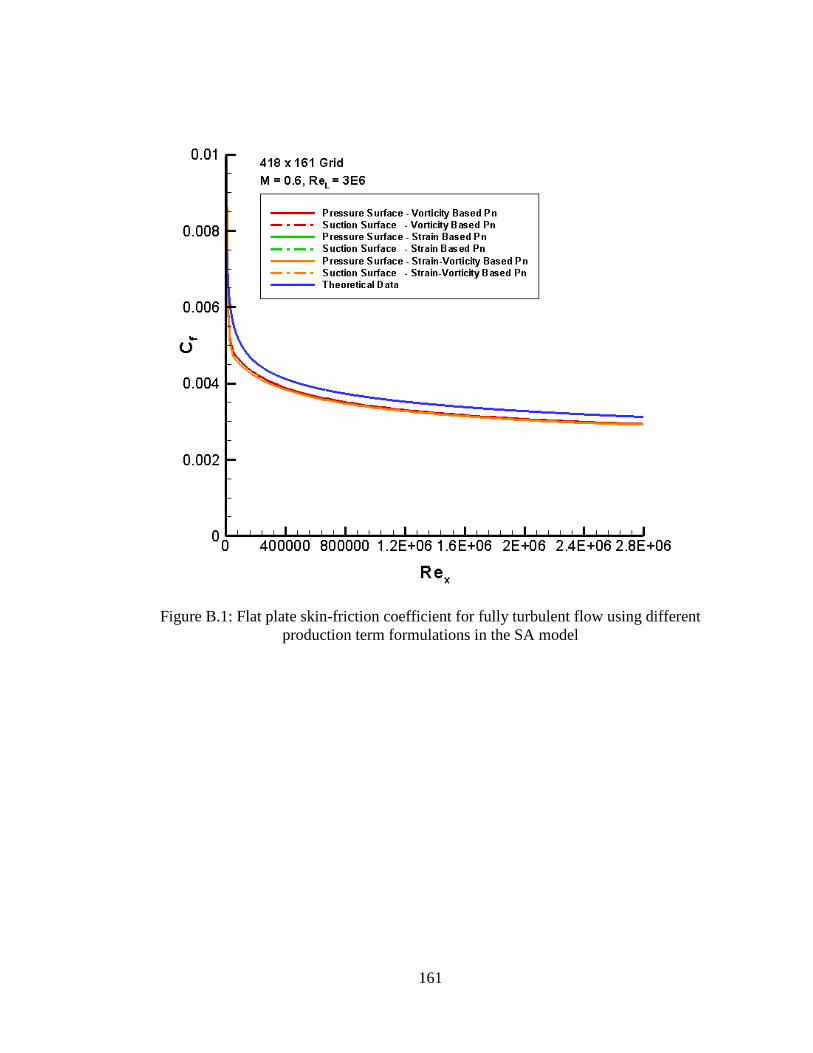
Appendix B: Turbulent Flat Plate Simulations at a Higher Mach Number............... 160
References....................................................................................................................... 163
Vita.................................................................................................................................. 166
Page 14
viii
LIST OF TABLES
Table 2.1 Airfoil and Cascade parameters (Buffum et al., 1998)................................. 9
Table 2.2 Flat plate airfoil grids.................................................................................. 17
Table 2.3 NASA-PW airfoil grids............................................................................... 18
Table 3.1 Baldwin-Lomax turbulence model constants.............................................. 23
Table 3.2 Spalart-Allmaras turbulence model constants............................................. 26
Table 5.1 Transitional flow parameters for the NASA-PW airfoil at the low incidence
angle condition............................................................................................ 90
Table 5.2 Transitional flow parameters for the NASA-PW airfoil at the low incidence
angle condition for different values of inlet turbulent viscosity............... 100
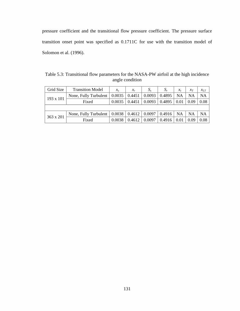
Table 5.3 Transitional flow parameters for the NASA-PW airfoil at the high incidence
angle condition.......................................................................................... 131
Table 5.4 Transitional flow parameters for the NASA-PW airfoil at the high incidence
angle condition for different values of inlet turbulent viscosity............... 134
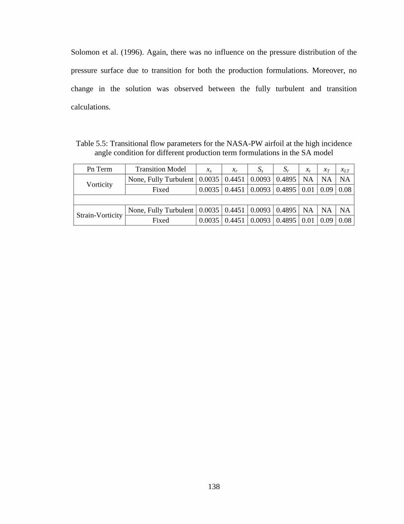
Table 5.5 Transitional flow parameters for the NASA-PW airfoil at the high incidence
angle condition for different production term formulations in the SA
model......................................................................................................... 138
Table 5.6 Transitional flow parameters for the NASA-PW airfoil at the high incidence
angle condition with and without streamline curvature correction........... 142
Table 5.7 Transitional flow parameters for the NASA-PW airfoil at the high incidence
angle condition for different values of inlet turbulent viscosity with
streamline curvature correction................................................................. 148
Page 15
ix
LIST OF FIGURES
Figure 2.1 Airfoil and cascade geometry....................................................................... 9
Figure 2.2 Chordwise distribution of y+ over the NASA-PW airfoil surface (193 x 101
Grid)............................................................................................................ 10
Figure 2.3 Example of a 3-D structured grid for an extruded NACA-0012 airfoil..... 12
Figure 2.4 Example of a 3-D unstructured grid for an extruded NACA-0012 airfoil. 13
Figure 2.5 An example of H-grid topology over a NACA-0012 airfoil....................... 14
Figure 2.6 C-grid around a NACA-0012 airfoil........................................................... 15
Figure 2.7 Example of O-grid around a NACA-0012 airfoil....................................... 16
Figure 2.8 Computational domain for the flat plate airfoil (238 x 164 Grid).............. 18
Figure 2.9 Computational domain for the NASA-PW airfoil (193 x 101 Grid).......... 19
Figure 2.10 Airfoil surface grid topology for the NASA-PW airfoil (193 x 101 Grid). 19
Figure 2.11 Grid topology in the leading edge region of the NASA-PW airfoil (193 x
101 Grid)..................................................................................................... 20
Figure 2.12 Grid topology in the trailing edge region of the NASA-PW airfoil (193 x
101 Grid)..................................................................................................... 20
Figure 3.1 Schematic diagram in a transitional flow with a separation bubble (Mayle,
1991)........................................................................................................... 32
Figure 4.1 Example of the variation of the intermittency factor in the transition region
over the suction surface of the NASA-PW airfoil (193 x 101 Grid).......... 37
Figure 5.1 Example of flat plate lift coefficient convergence history for laminar
flow............................................................................................................. 44
Figure 5.2 Example of the absolute value of the average density residual convergence
history for laminar flow over a flat plate airfoil.......................................... 45
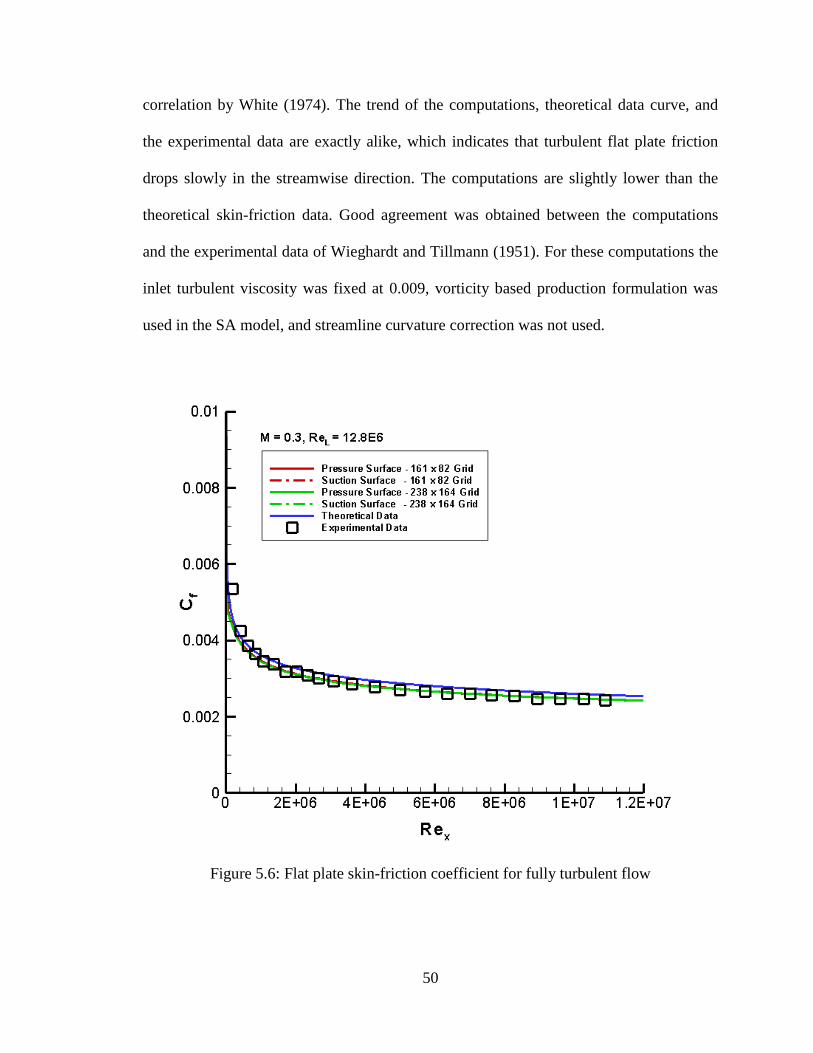
Figure 5.3 Flat plate skin-friction coefficient for laminar flow.................................... 47
Figure 5.4 Example of flat plate lift coefficient convergence history for fully turbulent
flow............................................................................................................. 48
Figure 5.5 Example of the absolute value of the average density residual convergence
history for fully turbulent flow over a flat plate airfoil............................... 49
Figure 5.6 Flat plate skin-friction coefficient for fully turbulent flow......................... 50
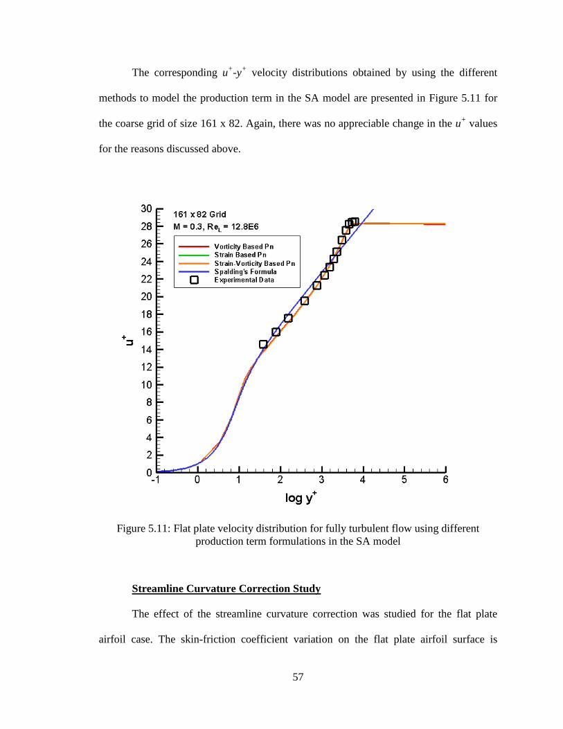
Figure 5.7 Flat plate velocity distribution for fully turbulent flow.............................. 52
Page 16
x
Figure 5.8 Flat plate skin-friction coefficient for fully turbulent flow with different
values of the inlet turbulent viscosity and initial conditions....................... 53
Figure 5.9 Flat plate velocity distribution for fully turbulent flow with different inlet
turbulent viscosity values and initial conditions......................................... 54
Figure 5.10 Flat plate skin-friction coefficient for fully turbulent flow using different
production term formulations in the SA model.......................................... 56
Figure 5.11 Flat plate velocity distribution for fully turbulent flow using different
production term formulations in the SA model.......................................... 57
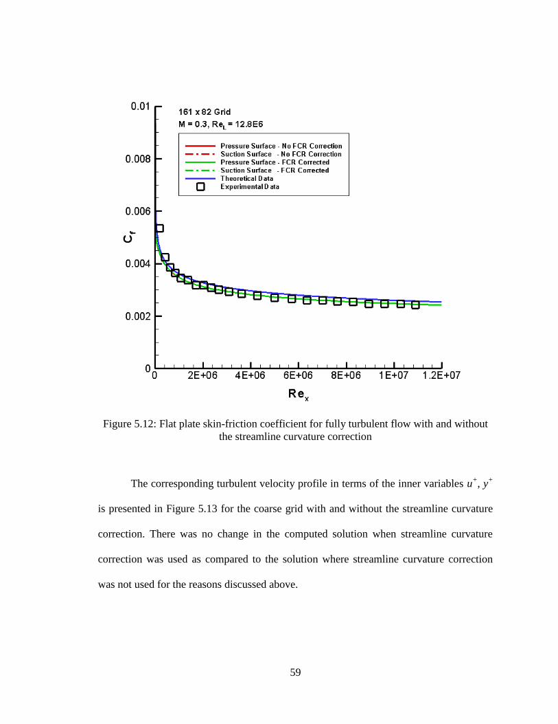
Figure 5.12 Flat plate skin-friction coefficient for fully turbulent flow with and without
the streamline curvature correction............................................................. 59
Figure 5.13 Flat plate velocity distribution for fully turbulent flow with and without the
streamline curvature correction................................................................... 60
Figure 5.14 Example of flat plate lift coefficient convergence history for turbulent and
transition flow............................................................................................. 61
Figure 5.15 Example of the absolute value of the average density residual convergence
history for turbulent and transition flow over a flat plate airfoil................ 62
Figure 5.16 Flat plate skin-friction coefficient for transition from laminar to turbulent
flow along the suction surface.................................................................... 64
Figure 5.17 Example of NASA-PW airfoil lift coefficient convergence history at the low
incidence angle condition for fully turbulent flow..................................... 66
Figure 5.18 Example of the absolute value of the average density residual convergence
history for the NASA-PW airfoil at the low incidence angle condition for
fully turbulent flow..................................................................................... 67
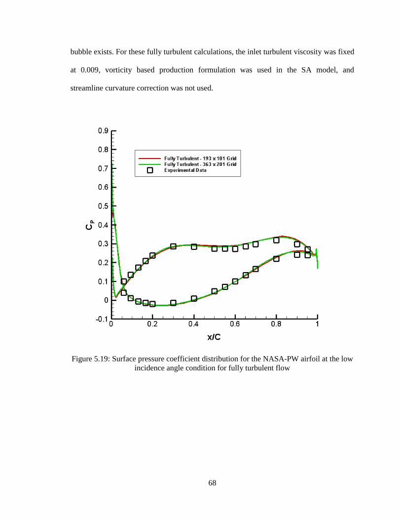
Figure 5.19 Surface pressure coefficient distribution for the NASA-PW airfoil at the low
incidence angle condition for fully turbulent flow..................................... 68
Figure 5.20 Leading edge surface pressure coefficient distribution for the NASA-PW
airfoil at the low incidence angle condition for fully turbulent flow......... 69
Figure 5.21 NASA-PW airfoil lift coefficient convergence history at the low incidence
angle condition for fully turbulent flow with the BL model providing the
initial conditions for the SA model............................................................. 71
Figure 5.22 Surface pressure coefficient distribution for the NASA-PW airfoil at the low
incidence angle condition for fully turbulent flow with the BL model
providing the initial conditions for the SA model...................................... 72
Figure 5.23 Leading edge surface pressure coefficient distribution for the NASA-PW
airfoil at the low incidence angle condition for fully turbulent flow with the
BL model providing the initial conditions for the SA model..................... 73
Page 17
xi
Figure 5.24 Surface pressure coefficient distribution for the NASA-PW airfoil at the low
incidence angle condition for fully turbulent flow with different inlet
turbulent viscosity values............................................................................ 75
Figure 5.25 Leading edge surface pressure coefficient distribution for the NASA-PW
airfoil at the low incidence angle condition for fully turbulent flow with
different inlet turbulent viscosity values..................................................... 76
Figure 5.26 Surface pressure coefficient distribution for the NASA-PW airfoil at the low
incidence angle condition for fully turbulent flow with and without the
streamline curvature correction................................................................... 78
Figure 5.27 Leading edge surface pressure coefficient distribution for the NASA-PW
airfoil at the low incidence angle condition for fully turbulent flow with and
without the streamline curvature correction................................................ 79
Figure 5.28 Streamlines in the leading edge region of the NASA-PW airfoil (193 x 101
Grid) at the low incidence angle condition for fully turbulent flow (a)
without streamline curvature correction, and (b) with streamline curvature
correction..................................................................................................... 80
Figure 5.29 Example of NASA-PW airfoil lift coefficient convergence history at the low
incidence angle condition for turbulent and transitional flow.................... 82
Figure 5.30 Example of the absolute value of the average density residual convergence
history for the NASA-PW airfoil at the low incidence angle condition for
turbulent and transitional flow.................................................................... 83
Figure 5.31 Contours of ρu for the NASA-PW airfoil (193 x 101 Grid) at the low
incidence angle condition for transitional flow using fixed transition onset
with xLT = 0.03............................................................................................ 85
Figure 5.32 Contours of ρu in the leading edge region of the NASA-PW airfoil (193 x
101 Grid) at the low incidence angle condition for transitional flow using
fixed transition onset with xLT = 0.03......................................................... 85
Figure 5.33 Velocity vectors with ρu contours in the leading edge region of the NASA-
PW airfoil (193 x 101 Grid) at the low incidence angle condition for (a)
fully turbulent flow, and (b) transitional flow using fixed transition onset
with xLT = 0.03............................................................................................ 86
Figure 5.34 Surface pressure coefficient distribution for the NASA-PW airfoil at the low
incidence angle condition for transitional flow using fixed transition onset
with xLT = 0.01............................................................................................ 91
Figure 5.35 Leading edge surface pressure coefficient distribution for the NASA-PW
airfoil at the low incidence angle condition for transitional flow using fixed
transition onset with xLT = 0.01................................................................... 92
Page 18
xii
Figure 5.36 Surface pressure coefficient distribution for the NASA-PW airfoil at the low
incidence angle condition for transitional flow using fixed transition onset
with xLT = 0.02............................................................................................. 93
Figure 5.37 Leading edge surface pressure coefficient distribution for the NASA-PW
airfoil at the low incidence angle condition for transitional flow using fixed
transition onset with xLT = 0.02................................................................... 94
Figure 5.38 Surface pressure coefficient distribution for the NASA-PW airfoil at the low
incidence angle condition for transitional flow using fixed transition onset
with xLT = 0.03............................................................................................. 95
Figure 5.39 Leading edge surface pressure coefficient distribution for the NASA-PW
airfoil at the low incidence angle condition for transitional flow using fixed
transition onset with xLT = 0.03................................................................... 96
Figure 5.40 Surface pressure coefficient distribution for the NASA-PW airfoil at the low
incidence angle condition for transitional flow using Mayle‟s transition
length model................................................................................................ 97
Figure 5.41 Leading edge surface pressure coefficient distribution for the NASA-PW
airfoil at the low incidence angle condition for transitional flow using
Mayle‟s transition length model.................................................................. 98
Figure 5.42 Surface pressure coefficient distribution for the NASA-PW airfoil at the low
incidence angle condition for transitional flow using fixed transition onset
with xLT = 0.01 for different inlet turbulent viscosity values.................... 101
Figure 5.43 Leading edge surface pressure coefficient distribution for the NASA-PW
airfoil at the low incidence angle condition for transitional flow using fixed
transition onset with xLT = 0.01 for different inlet turbulent viscosity
values......................................................................................................... 102
Figure 5.44 Velocity vectors with ρu contours in the leading edge region of the NASA-
PW airfoil (193 x 101 Grid) at the low incidence angle condition for the
inlet turbulent viscosity value of 0.009 for (a) fully turbulent flow, and (b)
transitional flow using fixed transition onset with xLT = 0.01................... 103
Figure 5.45 Velocity vectors with ρu contours in the leading edge region of the NASA-
PW airfoil (193 x 101 Grid) at the low incidence angle condition for the
inlet turbulent viscosity value of 10.0 for (a) fully turbulent flow, and (b)
transitional flow using fixed transition onset with xLT = 0.01................... 104
Figure 5.46 Example of NASA-PW airfoil lift coefficient convergence history at the
high incidence angle condition for fully turbulent flow............................ 106
Figure 5.47 Example of the absolute value of the average density residual convergence
history for the NASA-PW airfoil at the high incidence angle condition for
fully turbulent flow.................................................................................... 107
Page 19
xiii
Figure 5.48 Surface pressure coefficient distribution for the NASA-PW airfoil at the
high incidence angle condition for fully turbulent flow............................ 109
Figure 5.49 Leading edge surface pressure coefficient distribution for the NASA-PW
airfoil at the high incidence angle condition for fully turbulent flow....... 110
Figure 5.50 NASA-PW airfoil lift coefficient convergence history at the high incidence
angle condition for fully turbulent flow with the BL model providing the
initial conditions for the SA model........................................................... 112
Figure 5.51 Surface pressure coefficient distribution for the NASA-PW airfoil at the
high incidence angle condition for fully turbulent flow with the BL model
providing the initial conditions for the SA model..................................... 113
Figure 5.52 Leading edge surface pressure coefficient distribution for the NASA-PW
airfoil at the high incidence angle condition for fully turbulent flow with the
BL model providing the initial conditions for the SA model.................... 114
Figure 5.53 Surface pressure coefficient distribution for the NASA-PW airfoil at the
high incidence angle condition for fully turbulent flow with different inlet
turbulent viscosities................................................................................... 116
Figure 5.54 Leading edge surface pressure coefficient distribution for the NASA-PW
airfoil at the high incidence angle condition for fully turbulent flow with
different inlet turbulent viscosities............................................................ 117
Figure 5.55 Surface pressure coefficient distribution for the NASA-PW airfoil at the
high incidence angle condition for fully turbulent flow using different
production term formulations in the SA model......................................... 119
Figure 5.56 Leading edge surface pressure coefficient distribution for the NASA-PW
airfoil at the high incidence angle condition for fully turbulent flow using
different production term formulations in the SA model.......................... 120
Figure 5.57 Surface pressure coefficient distribution for the NASA-PW airfoil at the
high incidence angle condition for fully turbulent flow with and without
streamline curvature correction................................................................. 122
Figure 5.58 Leading edge surface pressure coefficient distribution for the NASA-PW
airfoil at the high incidence angle condition for fully turbulent flow with
and without streamline curvature correction............................................. 123
Figure 5.59 Example of NASA-PW airfoil lift coefficient convergence history at the
high incidence angle condition for turbulent flow with transition............ 124
Figure 5.60 Example of the absolute value of the average density residual convergence
history for the NASA-PW airfoil at the high incidence angle condition for
turbulent flow with transition.................................................................... 125
Page 20
xiv
Figure 5.61 Example of ρu contours for the NASA-PW airfoil (193 x 101 Grid) at the
high incidence angle condition for transitional flow using fixed transition
onset with xLT = 0.08................................................................................. 127
Figure 5.62 Example of ρu contours in the leading edge region of the NASA-PW airfoil
(193 x 101 Grid) at the high incidence angle condition for transitional flow
using fixed transition onset with xLT = 0.08.............................................. 127
Figure 5.63 Example of velocity vectors with ρu contours in the leading edge region of
the NASA-PW airfoil (193 x 101 Grid) at the high incidence angle
condition for (a) fully turbulent flow, and (b) transitional flow using fixed
transition onset with xLT = 0.08................................................................. 128
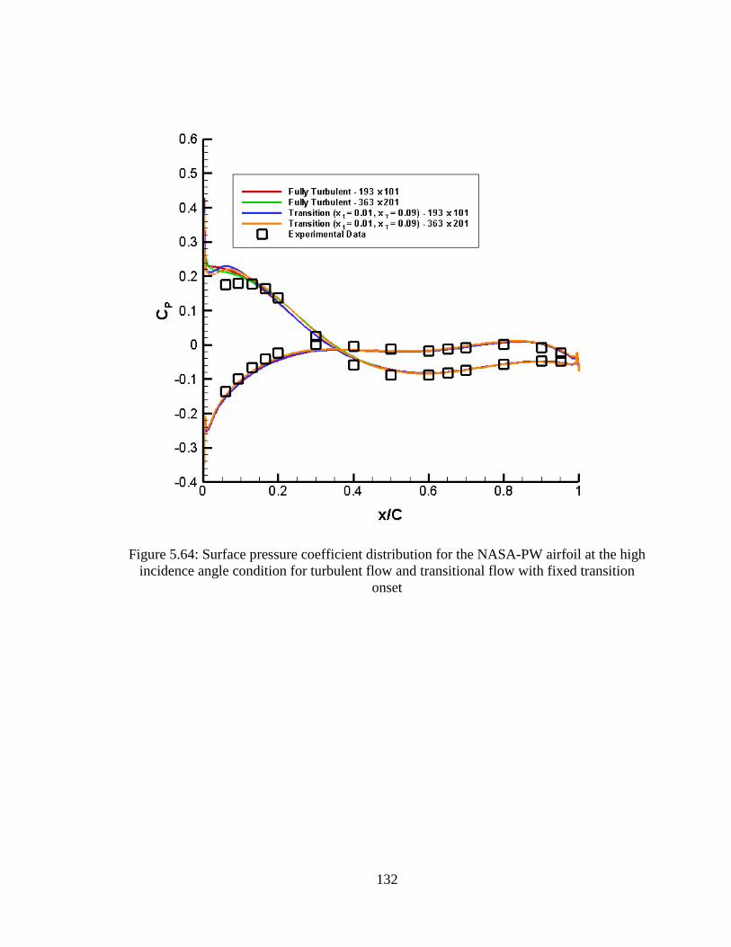
Figure 5.64 Surface pressure coefficient distribution for the NASA-PW airfoil at the
high incidence angle condition for turbulent flow and transitional flow with
fixed transition onset................................................................................. 132
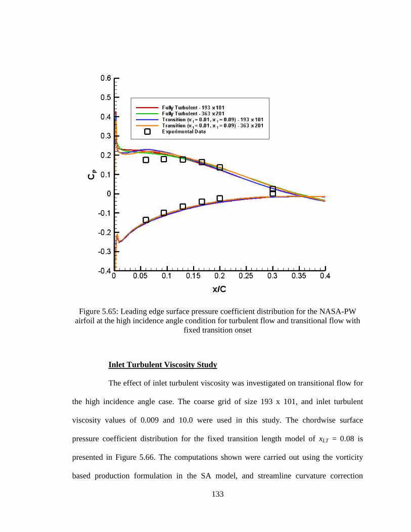
Figure 5.65 Leading edge surface pressure coefficient distribution for the NASA-PW
airfoil at the high incidence angle condition for turbulent flow and
transitional flow with fixed transition onset.............................................. 133
Figure 5.66 Surface pressure coefficient distribution for the NASA-PW airfoil at the
high incidence angle condition for turbulent flow and transitional flow with
fixed transition onset for different inlet turbulent viscosities.................... 135
Figure 5.67 Leading edge surface pressure coefficient distribution for the NASA-PW
airfoil at the high incidence angle condition for turbulent flow and
transitional flow with fixed transition onset for different inlet turbulent
viscosities.................................................................................................. 136
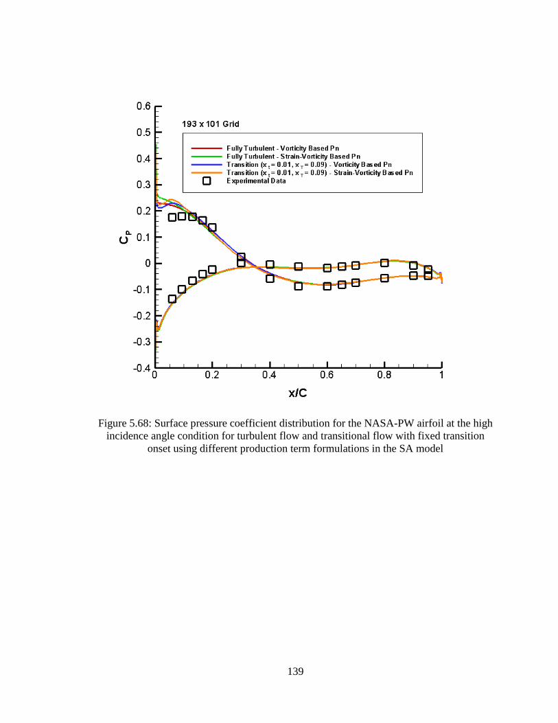
Figure 5.68 Surface pressure coefficient distribution for the NASA-PW airfoil at the
high incidence angle condition for turbulent flow and transitional flow with
fixed transition onset using different production term formulations in the SA
model......................................................................................................... 139
Figure 5.69 Leading edge surface pressure coefficient distribution for the NASA-PW
airfoil at the high incidence angle condition for turbulent flow and
transitional flow with fixed transition onset using different production term
formulations in the SA model................................................................... 140
Figure 5.70 Surface pressure coefficient distribution for the NASA-PW airfoil at the
high incidence angle condition for turbulent flow and transitional flow with
fixed transition onset with and without streamline curvature correction...143
Figure 5.71 Leading edge surface pressure coefficient distribution for the NASA-PW
airfoil at the high incidence angle condition for turbulent flow and
transitional flow with fixed transition onset with and without streamline
curvature correction................................................................................... 144
Page 21
xv
Figure 5.72 Streamlines in the leading edge region of the NASA-PW airfoil (193 x 101
Grid) at the high incidence angle condition with streamline curvature
correction for (a) fully turbulent flow, and (b) transitional flow using fixed
transition onset with xLT = 0.08................................................................. 145
Figure 5.73 Surface pressure coefficient distribution for the NASA-PW airfoil at the
high incidence angle condition for turbulent flow and transitional flow with
fixed transition onset for different inlet turbulent viscosities with streamline
curvature correction................................................................................... 149
Figure 5.74 Leading edge surface pressure coefficient distribution for the NASA-PW
airfoil at the high incidence angle condition for turbulent flow and
transitional flow with fixed transition onset for different inlet turbulent
viscosities with streamline curvature correction....................................... 150
Page 22
xvi
LIST OF SYMBOLS
, , , CMUTM,
constants in the Baldwin-Lomax model
, , , , , ,
, , , empirical constants in the Spalart-Allmaras model
C airfoil chord
skin-friction coefficient
pressure coefficient
constant in the curvature and rotation sensitization
lift coefficient
distance to the wall (Spalart-Allmaras model)
, , , , empirical functions in the Spalart-Allmaras model
function used to determine FMAX and yMAX in the Baldwin-
Lomax model
function in the curvature and rotation sensitization
Klebanoff intermittency factor
maximum of function F(y) (Equation (3.8)) in the Baldwin-
Lomax model
variable in the Baldwin-Lomax model
, , intermediate variables in the Spalart-Allmaras model
components of acceleration due to gravity (i = 1, 2, 3)
factor dependent on the grid for the transition term in the
Spalart-Allmaras model
h blade height
i, j, k grid point indices
acceleration parameter, Clauser constant
Page 23
xvii
algebraic length scale in the Baldwin-Lomax model
lift force, airfoil chord
M inlet Mach number
pressure
pressure in the free stream, inlet pressure
Pn turbulence production term in the Spalart-Allmaras model
local Reynolds number
Reynolds number between the point of separation and
transition onset
Reynolds number between the length of transition
Reynolds number based on chord
Reynolds number based on momentum thickness at the point
of separation
Richardson number
s strain rate
Δs non-dimensional spacing of the first grid point off the airfoil
surface
S airfoil spacing or pitch, measure of the deformation tensor in
the Spalart-Allmaras model
strain rate tensor (i, j = 1, 2, 3)
Sr streamwise point of flow reattachment
Ss streamwise point of flow separation
time
tmax maximum thickness of the airfoil
, velocity components
velocity vector
Page 24
xviii
instantaneous velocity components (i = 1, 2, 3)
difference between the maximum and minimum velocity
magnitude in the profile (Baldwin-Lomax model)
u∞, , free stream velocity or inlet velocity
friction velocity
, law-of-the-wall variables
mean flow velocity
norm of the difference between the velocity at the trip and
that at the field point (Spalart-Allmaras model)
mean velocity components (i = 1, 2, 3)
mean velocity components (j = 1, 2, 3)
free stream velocity at the point of separation
x, y, z Cartesian coordinates in physical space
x, X chordal distance in the x direction
streamwise coordinate
grid spacing along the wall at the trip (Spalart-Allmaras
model)
Cartesian coordinates (i = 1, 2, 3)
Cartesian coordinates (j = 1, 2, 3)
xmax location of maximum thickness of the airfoil
xpitch, ypitch Cartesian coordinate of the pitching axis location
streamwise point of flow reattachment, chordal distance of
the point of flow reattachment (Tables in Chapter 5)
streamwise point of flow separation, chordal distance of the
point of flow separation (Tables in Chapter 5)
streamwise distance between the point of separation and
transition onset
Page 25
xix
streamwise point of transition onset
streamwise length of transition
streamwise point of transition termination
X, Y, Z Cartesian coordinates in physical space
coordinate normal to solid surface
value of y at which F(y) (Equation (3.8)) is maximum
(Baldwin-Lomax model)
Y chordal distance in the y direction
mean incidence relative to the airfoil chord line
intermediate variable in the Spalart-Allmaras model
boundary layer thickness
Kronecker delta function
strain rate tensor
intermittency factor
von Kármán constant
viscosity
effective turbulent (or eddy) viscosity
μt turbulent (or eddy) viscosity
kinematic viscosity
kinematic viscosity at the point of separation
kinematic turbulent (or eddy) viscosity
modified turbulent (or eddy) kinematic viscosity in the
Spalart-Allmaras model
vorticity
Page 26
xx
vorticity at the wall at the trip point (Spalart-Allmaras
model)
vorticity tensor (i, j = 1, 2, 3)
density
density in the free stream, inlet density
turbulent Prandtl number
shear stress at the wall
momentum thickness at the point of separation
* leading edge camber angle
stagger angle
ξ, η, ζ coordinates in the computational space
Page 27
xxi
LIST OF FILES
File Name File Size
1. Vivek_Hariharan_thesis.pdf................................................................................3.5 MB
Page 28
1
Chapter One
Introduction
Background
Almost every flow in nature and in practical engineering applications is turbulent.
After years of research in turbulence, there still does not exist a precise definition of
turbulence. However, some of the characteristics of turbulent flows can be listed:
irregularity, diffusivity, large Reynolds numbers, three-dimensional vorticity fluctuations,
and dissipation (Tennekes and Lumley, 1972). Inspite of all the uncertainties associated
with turbulent flows, it has been encouraging that engineering calculations have been
possible with well-formulated turbulence models.
In 1937, Taylor and von Kármán proposed the following definition of turbulence:
“Turbulence is an irregular motion which in general makes its appearance in fluids,
gaseous or liquid, when they flow past solid surfaces or even when neighbouring streams
of the same fluid flow past or over one another” (Wilcox, 1994). Turbulence is usually
characterized by the presence of a wide range of length and time scales (Wilcox, 1994).
The Navier-Stokes (NS) equation, in its general form, has been around for two
centuries now.
The NS equation combined with the continuity and energy equations describe the motion
of fluid substances. These equations describe how the velocity, pressure, energy, and
density of a moving fluid are related. The viscosity, μ, is a function of the thermodynamic
state, and for most fluids displays a strong dependence on temperature. However, if the
Page 29
2
temperature differences are not very large within the fluid, then μ can be regarded as a
constant.
Another important flow characteristic of fluid flow is transition to turbulence.
Transition is the process by which a laminar flow changes to a turbulent flow. It is known
that, typically, the boundary layer flow is laminar over the surface of the body before it
transitions to turbulent flow due to flow instabilities. Instability of a laminar flow does
not immediately lead to turbulence, which is a severely nonlinear and chaotic stage
characterized by macroscopic “mixing” of fluid particles. Some of the transition modes
which lead to turbulence are natural transition, bypass transition, or separated flow
transition. The discussion below on these different transition modes is a summary of what
appears in Mayle (1991).
In the process for natural transition, after the initial breakdown of laminar flow
occurs because of amplification of small disturbances, the flow goes through a complex
sequence of changes finally resulting in the chaotic state known as turbulence. Natural
transition occurs when the laminar boundary layer becomes susceptible to small
disturbances, which grow into an instability. This instability amplifies within the layer to
a point where it grows and develops into loop vortices with large fluctuations. These
highly fluctuating loop vortices inside the laminar boundary layer develop into turbulent
spots, which then are convected downstream, and eventually, with time, grow and
coalesce to form a fully developed turbulent boundary layer.
Bypass transition usually occurs at high free-stream turbulence levels. In this
mode of transition, free-stream disturbances influence the development of turbulent spots
that are directly produced within the boundary layer.
Page 30
3
Separated-flow transition occurs in the laminar separation bubble. The flow
transitions into turbulent flow over the separated bubble and reattaches to the surface
forming a turbulent shear layer. This usually occurs in an adverse pressure gradient
region that contributes to the separation of the laminar boundary layer. Separated flow
transition is usually found on the suction surface, near a compressor airfoil‟s leading
edge, or near the point of minimum pressure. Turbine blades are likely to have separation
along the suction surface in the trailing edge region. High levels of free-stream turbulence
can cause early transition compared to lower turbulence levels.
In gas turbine engines, the flow is periodically unsteady, so is transition, and this
is called periodic-unsteady transition. In “wake-induced” transition, the periodic passing
of wakes from the upstream blades or obstructions causes unsteadiness in the flow field
and affects transition on the downstream blades.
There also exists something called reverse transition, i.e., transition from turbulent
to laminar flow, which is referred to as “relaminarization.” This is usually expected to
occur at low turbulence levels if the acceleration parameter, , is
greater than 3 x 10⁻⁶
. In this equation, U refers to the velocity in the streamwise direction
and x refers to the surface coordinate in the streamwise direction.
Predicting transition becomes very important for improving the efficiencies of gas
turbine engines. Considering transition will lead to improved designs of turbomachinery
airfoils. A significant amount of research effort has been devoted to determine the
transition regime inside the boundary layer. Since Direct Numerical Simulation (DNS)
and Large Eddy Simulation (LES) are more computationally expensive using present
computing hardware, the Reynolds-Averaged Navier-Stokes (RANS) equations continue
Page 31
4
to be better suited for engineering calculations with the incorporation of appropriate
turbulence and transition models.
Literature Review
The incorporation of transition models into existing RANS solvers is an area of
fundamental research interest. The Chen and Thyson (1971) model has been used by
Ekaterinaris et al. (1995) and van Dyken et al. (1996) in a thin layer RANS code for
transition calculations of steady (stationary) and oscillating airfoils. An adjustment of the
Chen-Thyson transition constant was necessary to get better correlation with
experimental data since the basis of this constant was on zero pressure gradient flow.
Solomon et al. (1996) developed a relationship that considers the influence of
pressure gradients as well as free-stream turbulence intensity on transition length for
attached flow. Sanz and Platzer (1998) used the Solomon et al. (1996) transition model
for transitional flow calculations. Computations were performed on separation bubbles
for a NACA0012 airfoil and found that the Solomon et al. transition model successfully
predicted the NACA0012 airfoil separation bubbles. This work was continued by Sanz
and Platzer (2002) to determine the influence of turbulence models and discretization
methods on transition predictions.
Suzen et al. (2003) developed a transition model by combining the models of
Steelant and Dick (1996) and Cho and Chung (1992) to solve a transport equation for the
intermittency factor. Suzen et al. found that the intermittency thus obtained reproduced
the experimentally observed streamwise variation of the intermittency in the transition
region, and could also provide a realistic picture of normal-to-wall variation of the
Page 32
5
intermittency profile. Using this transition model, good overall agreement of the
computational predictions with the experimental data was demonstrated.
Langtry and Sjolander (2002) proposed a transition model for predicting the onset
of transition by taking into account the influence of freestream turbulence intensity,
pressure gradient and flow separation. The model was based on the concept of vorticity
Reynolds number (proposed by Van Driest and Blumer, 1963) and calibrated for use with
the Menter SST turbulence model. Langtry and Sjolander used their transition model on
different test cases and demonstrated good agreement with the experiments as compared
to laminar and turbulent solutions.
The majority of transition models depend on boundary layer parameters. This
makes transition models difficult to apply to three dimensional flows and advanced
Computational Fluid Dynamics (CFD) codes that use unstructured grids. To overcome
this difficulty, Menter et al. (2002) developed a correlation-based method with a general
transport equation that depends on local variables. This approach has been extended by
Menter et al. (2006) to include two transport equations, one for intermittency and one for
the transition onset criteria through use of the momentum thickness Reynolds number.
Application of this approach to a number of different test cases yielded promising results.
Recently Whitlow et al. (2006) used a three dimensional RANS code and a two
dimensional RANS code with the Solomon et al. (1996) transition model to predict the
flow for the NASA-Glenn Research Center (GRC) Transonic Flutter Cascade (TFC)
airfoil. Steady flow computations were performed for both the low and large incidence
angle cases for which surface pressure measurements are available. Distinct leading edge
separation bubbles were predicted for each incidence angle. In particular, for the large
Page 33
6
incidence case, improved correlation with the measurements was exhibited compared to
the fully turbulent calculations.
Objectives
The overall objective of this research is to predict the transitional flow regime for
steady flow over a transonic compressor (NASA-PW) airfoil cross-section. The
numerical results obtained are correlated with the experimental data obtained from the
Transonic Flutter Cascade (TFC) at NASA Glenn Research Center (GRC). The effect of
different transition lengths and transition onset models on the steady pressure distribution
is studied. The investigation is done for a low incidence angle and a high incidence angle
condition. The high incidence angle condition has a large separation bubble on the
suction surface in the leading edge region.
In particular, computational studies are done for turbulent and transitional flow on
a flat plate airfoil, and the NASA-PW airfoil. The turbulent flow predictions use the
Spalart-Allmaras (SA) (1994) one-equation turbulence model. The transitional flow
predictions use the intermittency correlation given by Dhawan and Narasimha (DN)
(1958) for fixed transition length and Mayle‟s (1991) transition length model. The DN
model was selected because the transition onset location and transition length could be
varied independently.
In this research, the flat plate studies are crucial in order to validate the
implementation of the numerical scheme. Since experimental data for turbulent and
transitional flows over flat plates are readily available, the numerical results obtained are
correlated with this data. The effect of inlet turbulent viscosity is also quantified for the
Page 34
7
SA model. In addition, the effect of turbulence production in the SA model is also
investigated by using the mean-strain rate based production, blended mean-strain rate and
vorticity based production, and the classical vorticity based production. Moreover,
streamline curvature effect is also studied by sensitizing the SA model to such effects.
Furthermore, a new approach to speed up the convergence of the solution for the NASA-
PW airfoil has been explored by combining the Baldwin-Lomax (BL) (1978) algebraic
turbulence model and the SA model.
Page 35
8
Chapter Two
Geometry and Grid Generation
Cascade Geometry
The experimental data for this work was generated in the NASA-GRC TFC
(Buffum et al., 1998). An exhaust system was used to draw atmospheric air through
honeycomb into a smoothly contracting inlet section; test section Mach numbers up to
1.15 were possible. Downstream of the inlet was a rectangular duct that contained the
nine airfoil test section. This facility had the unique capability of oscillating the nine
airfoils simultaneously at a specified interblade phase angle using a high-speed cam
driven system at frequencies up to 550 Hz. The experimental data used in this work were
acquired at an inlet Mach number of 0.5 with a chordal Reynolds number of 0.9 Million
for a low and high incidence angle condition.
To reduce the boundary layer thickness, suction was applied to the cascade side
walls through perforated walls upstream of the test section. The tailboards used to control
the test section exit pressure also formed bleed scoops to reduce the upper and lower wall
boundary layers. Chordwise surface static pressure taps were located at mid-span (52%
span) as well as 35% and 17.5% span. For the high incidence angle condition, the
chordwise pressure distributions at each span location were nearly identical with a slight
deviation at the 17.5% span location for the static pressure measurement nearest to the
airfoil leading edge. Flow visualization using an oil-pigment mixture indicated that at the
high incidence angle condition the flow was separated at mid-span from the leading edge
to 40% chord. The separated flow region did decrease in chordwise extent to
approximately 7% chord near the upper and lower walls. Based on the experimental
Page 36
9
results a two-dimensional analysis was pursued of the mid-span region of the cascade
airfoils.
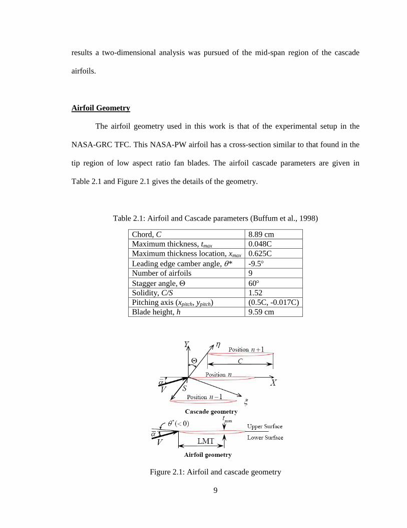
Airfoil Geometry
The airfoil geometry used in this work is that of the experimental setup in the
NASA-GRC TFC. This NASA-PW airfoil has a cross-section similar to that found in the
tip region of low aspect ratio fan blades. The airfoil cascade parameters are given in
Table 2.1 and Figure 2.1 gives the details of the geometry.
Table 2.1: Airfoil and Cascade parameters (Buffum et al., 1998)
Chord, C 8.89 cm
Maximum thickness, tmax 0.048C
Maximum thickness location, xmax 0.625C
Leading edge camber angle, * -9.5
Number of airfoils 9
Stagger angle, 60
Solidity, C/S 1.52
Pitching axis (xpitch, ypitch) (0.5C, -0.017C)
Blade height, h 9.59 cm
Figure 2.1: Airfoil and cascade geometry
Page 37
10
Grid Generation
The grids were generated using POINTWISE. The two dimensional grids have a
sheared H-mesh topology. The grids generated have the first grid point off the airfoil
surface so as to yield y+ values of order . Figure 2.2 below shows typical y
+ values
for the first grid point off the airfoil surface from the leading edge to the trailing edge of
the airfoil. The grids were generated in a manner so as to closely follow the airfoil surface
profile from the leading edge up to the trailing edge. It was ensured that the grid lines
emanating from the airfoil surface remain nearly orthogonal to the surface up to and
exceeding the boundary layer thickness. This guarantees that the grid cells close to the
airfoil surface are not skewed. The expansion ratio of the grid away from the airfoil
surface is maintained at a value of 1.2.
Figure 2.2: Chordwise distribution of y+ over the NASA-PW airfoil surface (193 x 101
Grid)
Page 38
11
Different Types of Grids
Before numerical solution of the governing equations can be generated, the flow
domain and its boundaries must be discretized. The choice of discretization is made
between structured and unstructured grids. Figure 2.3 presents an example of a structured
grid and Figure 2.4 shows an example of an unstructured grid. Both structured and
unstructured grids have their own specific advantages and disadvantages. Since the grids
used in this research are structured grids, the discussion below will be limited to
structured grids only.
The grid points in a structured grid are distinctively identified by a particular set
of indices i, j, k (one for each coordinate direction) and every grid point has the set of
Cartesian coordinates in physical space given by (xi,j,k, yi,j,k, zi,j,k). The set of coordinates in
the computational space is given by (ξi,j,k, ηi,j,k, ζi,j,k). The grid cells formed in a structured
grid are quadrilateral in shape in 2-D and hexahedral in shape in 3-D. The different types
of grid topologies that can be employed for structured grids are H-, C-, and O-grids.
Page 39
12
Figure 2.3: Example of a 3-D structured grid for an extruded NACA-0012 airfoil
Page 40
13
Figure 2.4: Example of a 3-D unstructured grid for an extruded NACA-0012 airfoil
Traditional H-grids and Sheared H-grids
The H-grid topology is most often employed for turbomachinery applications. The
H-grid topology is shown in Figure 2.5. As can be seen, the η = 0 and η = 1 grid lines
represent the periodic boundaries and the surfaces of the aerodynamic body. Moreover,
an η = const. grid line begins at the inlet boundary, which is located at ξ = 0, and ends at
the outlet boundary, which is located at ξ = 1.
In turbomachinery, the segments from the inlet boundary to the leading edge that
are represented by 1-3 and 2-4 are called the periodic boundaries since they are periodic
Page 41
14
to each other. In fact, they are rotationally periodic in 3-D. The same applies to the
segments 5-7 and 6-8. The grid points along the periodic boundaries should be placed in
such a way that they are clustered near the leading edge and trailing edge regions of the
blade. This is usually done by making the spacing of the first grid point along the periodic
boundary the same as that of the first grid point over the turbomachine blade‟s leading
and trailing edges, respectively. Segments 3-5 and 4-6 have solid-wall boundary
conditions.
The traditional H-grids have grid point distribution such as to yield symmetric
looking grid cells that are not distorted or skewed. Sheared H-grids distort the grid cells
near the leading edge and trailing edge of the airfoil‟s surface resulting in skewed looking
cells. In Figure 2.5, the traditional H-grid topology can be seen in the inlet and exit
portions of the grid, and in the mid-channel region between the airfoil surfaces. The
sheared H-grid topology can be seen near the leading edge and trailing edge regions of
the airfoil‟s surface. The grid point clustering along the boundaries of the grid and also
over the solid walls allows capturing the flow gradients accurately and to resolve the
viscous terms present in the NS equation and in any turbulence model. This allows the
cells to be stretched easily to account for different flow gradients in different directions.
Figure 2.5: An example of H-grid topology over a NACA-0012 airfoil
η = 1
η = 0
ξ = 0
ξ = 1 1
2
4
3
6
5
8
7
Airfoil Pressure Surface
Airfoil Suction Surface
Page 42
15
C-grids
C-grid topology around an aerodynamic body consists of a family of grid lines
that wrap around the surface of the body and also form the wake region behind the body.
The C-grid topology is shown in Figure 2.6. The C-grid topology when generated
introduces a coordinate cut, as also seen in the figure. The coordinate cut requires
mapping a single grid point in the physical domain onto two grid points in the
computational domain. Using a C-grid topology around an aerodynamic body, in general,
reduces skewness of the grid cells on the whole domain when compared to H-grids. In
particular, grid skewness is reduced near the leading edge as the grid lines wrap around
the leading edge and closely follows the leading edge surface profile in a better way as
compared to the grid cells in H-grid topology. Grid cells with low values of skewness are
important to reduce numerical errors during computation. Now, due to the presence of the
coordinate cut emanating from the trailing edge, a periodic boundary condition is
preferred at the cut so that the flow variables and gradients remain continuous across the
cut.
Figure 2.6: C-grid around a NACA-0012 airfoil
Coordinate Cut
Page 43
16
O-grids
In the case of O-grids, a family of grid lines form closed loops around the
aerodynamic body. The O-grid topology is displayed in Figure 2.7. The other family of
grid lines traverse in the radial direction away from the body and towards the outer
boundary. Again, as was found with the C-grids, generating an O-grid for an airfoil
creates a coordinate cut as shown in the Figure 2.7. An O-grid around the airfoil surface
resolves the boundary layer region near the surface in a much better manner by closely
following the surface profile of the airfoil. However, an airfoil with a sharp trailing edge
having an O-grid topology affects the grid quality in that region. Moreover, as with C-
grids, difficulty arises to keep the flow variables and their gradients continuous across the
cut and a periodic boundary is always preferred.
Figure 2.7: Example of O-grid around a NACA-0012 airfoil
Coordinate Cut
Page 44
17
Grids for Flat Plate Studies
Table 2.2 lists the essential features of the grids used for flat plate studies.
Table 2.2: Flat plate airfoil grids
Grid Size Δs Inlet Boundary Exit Boundary S/C
161 x 82 5.0E-6 2C 2C 10 0°
238 x 164 1.0E-6 2C 2C 1 0°
418 x 161 1.0E-5 2C 3C 1 0°
The grid size represents the number of grid points in the „x‟ and „y‟ directions
corresponding to „i‟ and „j‟ directions, respectively. A typical flat plate grid is shown in
Figure 2.8. The non-dimensional spacing of the first grid point off the airfoil surface is
given by Δs. The values for the inlet and exit boundaries represent the non-dimensional
distance at which the boundaries are located from the leading edge and the trailing edge
of the airfoil, respectively. The ratio S/C is the space-chord ratio and is the inverse of
solidity of the airfoil. The stagger angle of the flat plate airfoil cascade is represented by
Θ.
Page 45
18
Figure 2.8: Computational domain for the flat plate airfoil (238 x 164 Grid)
Grids for NASA-PW Airfoil
Table 2.3 lists the essential features of the grids used for NASA-PW airfoil.
Table 2.3: NASA-PW airfoil grids
Grid Size Δs Inlet Boundary Exit Boundary S/C
193 x 101 5.0E-6 3C 3C 0.65789 60°
363 x 201 5.0E-6 3C 3C 0.65789 60°
The discussion immediately following Table 2.2 also applies to Table 2.3. Some
typical views of the grids used in this research are displayed below in Figures 2.9 through
Airfoil Surface
Airfoil Surface
Inle
t
Ou
tlet
S C
Page 46
19
2.12. The grid distribution near the airfoil surface is such that it resolves the boundary
layer region effectively by having the grid points move away from the surface in a
geometric fashion. The coarse grid of size 193 x 101 has 85 grid points over the airfoil
surface, and the dense grid of size 363 x 201 has 182 grid points over the airfoil surface.
Grid independence of fully turbulent and transition solutions were demonstrated using
these grids.
Figure 2.9: Computational domain for the NASA-PW airfoil (193 x 101 Grid)
Figure 2.10: Airfoil surface grid topology for the NASA-PW airfoil (193 x 101 Grid)
Inlet Boundary Periodic Boundaries
Exit Boundary
Suction Surface
Pressure Surface
Suction Surface
Pressure Surface
S
C
Page 47
20
Figure 2.11: Grid topology in the leading edge region of the NASA-PW airfoil (193 x 101
Grid)
Figure 2.12: Grid topology in the trailing edge region of the NASA-PW airfoil (193 x 101
Grid)
Page 48
21
Chapter Three
Turbulence and Transition Models
Turbulence
It is now understood and accepted that turbulent flows are characterized by
varying length and time scales. The inherent nature of turbulent flow causes the velocity
field to fluctuate. This in turn yields rapid mixing of the transported quantities, such as
momentum and energy. To capture the exact physics of the flow, especially for the small-
scale high-frequency fluctuations, DNS of the governing equations is required. Since
DNS is too computationally expensive with present computing hardware for practical
engineering applications, other approaches, such as time-averaging or ensemble-
averaging of the instantaneous governing equations, are employed. However, the
modified equations contain additional unknown variables creating what is called the
turbulence „closure‟ problem. Hence, turbulence models are needed to determine these
additional variables. Reynolds averaging the NS equation introduces additional stress
terms, known as the Reynolds stress, which acts on the mean turbulent flow. Boussinesq
proposed to address these Reynolds stress terms by introducing what is called the
turbulent or eddy viscosity in a manner analogous to laminar shear stress.
Baldwin-Lomax Algebraic Turbulence Model
The Baldwin-Lomax (BL) (1978) model is a two-layer algebraic model (also
called a zero-equation model) which gives the eddy viscosity, μt, as a function of the local
boundary layer velocity profile. The eddy viscosity is calculated in this research by using
a blending function as proposed by Granville (1990) that is given by
Page 49
22
(3.1)
The Prandtl-Van Driest formulation is used in the inner region which gives
(3.2)
where
(3.3)
The magnitude of the vorticity, , for two dimensional flow is given by
(3.4)
and
(3.5)
For the outer region
(3.6)
where K is the Clauser constant, which is given with the other modeling constants in
Table 3.1.
(3.7)
The quantities yMAX and FMAX are determined from the maximum of the function
(3.8)
For computation in the wake region, the exponential term in F(y) is set to zero. The
Klebanoff intermittency factor, FKLEB(y), is given by
(3.9)
Page 50
23
The quantity uDIF is the difference between the maximum and minimum velocity
magnitude in the profile at a specific x location and is given by, for two dimensional flow,
(3.10)
For boundary layers, the minimum is always set to zero in the above equation.
The effect of transition from laminar to turbulent flow can be simulated by setting
μt to zero everywhere in a profile where the maximum computed value of μt is less than a
specified value, that is, μt = 0 if max(μt)profile < CMUTM u∞. However, this feature of the
Baldwin-Lomax model has not been implemented in the flow solver used for the purpose
of this research.
The constants in the Baldwin-Lomax model take the values presented in Table
3.1, as used by Chima, Giel, and Boyle (1993).
Table 3.1: Baldwin-Lomax turbulence model constants
A+
26
CCP 1.216
CKLEB 0.646
CWK 1
κ 0.4
K 0.0168
CMUTM 14
In the Baldwin-Lomax model, the distribution of vorticity is used to determine
length scales so that the necessity for finding the outer edge of the boundary layer is
Page 51
24
removed. The model is suitable for high-speed flows with thin attached boundary layers
(http://www.cfd-online.com/Wiki/Baldwin-Lomax_model, 2007). The Baldwin-Lomax
model was not developed for cases with large separation bubbles or significant
rotation/curvature effects.
The Baldwin-Lomax model requires a well-resolved grid near the walls, with the
first cell off the airfoil surface located at y+ < 1. The model does not always give accurate
solutions, especially for cases with large separation zones and recirculation. However, the
Baldwin-Lomax model can be used to provide a reasonable initial condition for more
sophisticated turbulence models.
Spalart-Allmaras One-Equation Turbulence Model
The Spalart-Allmaras (1994) model is a one-equation model that solves a
transport equation to determine the eddy viscosity to resolve the turbulence closure
problem. The transport equation is based on empiricism, dimensional analysis, Galilean
invariance, and dependence on the molecular viscosity. The model was calibrated using
two-dimensional mixing layers, wakes, and flat plate boundary layers. The model gives
satisfactory results for boundary layers subjected to pressure gradients.
The Spalart-Allmaras (SA) model solves for the transport variable, , which is a
modified form of the turbulent kinematic viscosity and obeys the transport equation
(3.11)
where
Page 52
25
(3.12)
(3.13)
(3.14)
(3.15)
(3.16)
(3.17)
(3.18)
(3.19)
(3.20)
(3.21)
(3.22)
Page 53
26
The constants in the SA model are given below in Table 3.2.
Table 3.2: Spalart-Allmaras turbulence model constants
σ 2/3
cb1 0.1355
cb2 0.622
cw1 (cb1/κ2) + (1+cb2)/σ
cw2 0.3
cw3 2
κ 0.41
cv1 7.1
ct1 1
ct2 2
ct3 1.2
ct4 0.5
The terms on the right-hand side of the transport equation represent eddy-viscosity
production, diffusion, and destruction. The effect of transition is also included through
the ft1ΔU2 term.
The production term, which is the first term on the right-hand side of the transport
equation, can be modified to improve the accuracy of the solution. The modification
applies to the scalar measure of the deformation tensor, S. The original SA model uses the
magnitude of vorticity, |ω| for S.
Page 54
27
(3.23)
where Ωij is the vorticity tensor given by
(3.24)
The argument that supports using |ω| for S is that, for aerodynamic flows for which the
model was formulated, turbulence is found only where vorticity is present near the solid
boundaries. The other possible choice for S is to base it on the magnitude of strain rate |s|
as indicated by Spalart and Allmaras (1994) and Dacles-Mariani et al. (1995).
(3.25)
where Sij is the strain rate tensor defined as
(3.26)
However, a new form for S has been proposed in Dacles-Mariani et al. (1995) that
combines both |ω| and |s| as follows:
(3.27)
where Cprod = 2. The motivation for this modification is that taking into account both
vorticity and strain rate reduces the eddy viscosity being generated in regions where the
vorticity exceeds the strain rate. This behavior can be seen at the core of a vortex where
pure rotation is taking place and consequently the turbulence should be suppressed
(Dacles-Mariani et al., 1995).
History effects are taken into account by the Spalart-Allmaras model, where the
convection and the diffusion of turbulence is modeled by the transport equation presented
above. This model is easy to implement on structured as well as unstructured grids.
Page 55
28
The capability of the Spalart-Allmaras model to yield smooth laminar-turbulent
transition at the point specified by the user is not used in the present work. An explicit
transition model is used in this research. Thus, the solution generated by using the
Spalart-Allmaras model only represents a fully turbulent solution right from the leading
edge.
Boundary and Initial Conditions for the Spalart-Allmaras Turbulence Model
To obtain a physical solution to the governing equations, appropriate initial and
boundary conditions need to be specified. The initial conditions provide the state of the
fluid at time t = 0.
In computer simulation of a physical flow domain, only a part of the physical
domain is considered. This results in truncation of the original flow domain and creates
non-physical boundaries, such as inlet boundaries, outlet boundaries, and periodic
boundaries. At these boundaries the values of the flow variables must be specified.
Moreover, the solution obtained on the truncated domain should represent the solution for
the entire physical domain.
The wall boundary condition for the SA model requires the modified turbulent
kinematic viscosity, , is zero. For the exit boundary, extrapolation from the interior of
the flow domain is used to specify the values at the boundary. At the inlet boundary, the
Dirichlet boundary condition is used that requires specifying the turbulent viscosity. For
the periodic boundaries, the values are specified using the periodicity condition. More
details concerning the inlet boundary condition and initial condition for the modified
turbulent viscosity for the SA model are given in the next section.
Page 56
29
Inlet Turbulent Viscosity and Initial Condition
The non-dimensional inlet turbulent viscosity in the SA model was previously
specified as 0.009 (CFL3D Version 5.0 User‟s Manual, 1997). In this research the
capability of specifying any desired inlet turbulent viscosity was added to the SA model.
This was accomplished through use of a set of correlations for converting the turbulent
eddy viscosity, νt, to the modified eddy viscosity in the SA model, , provided by Wong
(1999). The correlations are presented below.
(3.28)
where
(3.29)
(3.30)
(3.31)
(3.32)
(3.33)
The value of cv1 is the same as that in the SA model. The above correlations can be used
to specify and test the effect of different initial conditions of on the final solution.
Furthermore, the effect of specifying a fixed value of at the inlet boundary can be
investigated.
Page 57
30
The above procedure can also be used to generate better initial conditions for the
SA model by obtaining an initial solution with the BL model and utilizing the turbulent
viscosity, νt, calculated and converting it to the transformed eddy viscosity, , using the
relationships presented by Wong (1999).
Streamline Curvature Correction
Sensitization of the solution to the effects of streamline curvature can be studied
by implementing the model proposed by Hellsten (1998). In the present work, the
suggested model of Hellsten is incorporated into the SA turbulence model by effectively
modifying the turbulence production term of the SA model. The model equations are
presented below.
(3.34)
(3.35)
where CCR = 3.6, and the terms |ω| and |s| are the magnitude of vorticity and the
magnitude of strain rate, respectively, as given above. The Richardson number, Ri, which
is a dimensionless number indicates the level of turbulence in the flow with lower values
indicating significant turbulence. The FCR model has been calibrated for a rotating
channel flow (Hellsten, 1998). The term FCR sensitizes the SA turbulence model, which is
an eddy-viscosity model, for curvature/rotation effects. As recommended by Yaras and
Grosvenor (2003) the FCR term is multiplied by the production term in the SA model. In
the code used for the purpose of this research, the FCR correction of Hellsten has been
implemented as described above with the option of turning the FCR correction on/off.
Page 58
31
Transition from Laminar to Turbulent Flow
Emmons (1951) took the first major step in providing a description of the
transitional region in a boundary layer. He proposed that transition occurred through the
development of turbulent spots that were surrounded by laminar flow (Narasimha, 1985).
Previously, transition was thought to be an abrupt, more or less two-dimensional
discontinuity of laminar into turbulent flow (Mayle, 1991). In 1935, Prandtl said, “In
actual fact the transition is accomplished in a region of appreciable length and moreover
experiments show that the position of the point when turbulence commences oscillates
with time” (Narasimha, 1985). In recent times, the concept of transition as a randomly
intermittent laminar-turbulent flow has gained acceptance.
Mayle Transition Length Model
Based on experimental data for separated flow transition, Mayle (1991) suggested
the following correlation for determining the transition onset point, xt,
(3.36)
The Reynolds numbers, (Rex)st and Reθs, correspond to the Reynolds number between the
point of separation and transition onset, and the momentum thickness Reynolds number
at the point of separation, respectively, and are defined as
(3.37)
(3.38)
The above relations require that the conditions at the point of separation be known for
predicting the point of transition onset. A second experimental correlation is provided by
Mayle for determining the transition termination point, xT,
Page 59
32
(3.39)
Using the above relation, the length of the transition region, xT – xt, can be estimated. In
the correlations provided above for Mayle‟s transition length model, xs, xt, and xT
represent streamwise distances.
The important features of separated-flow transition over a separation bubble are
shown in Figure 3.1. As explained by Mayle (1991) in the upstream region, the laminar
shear flow zone becomes unstable, which leads to the formation of turbulent spots and the
onset of transition starts at this point. The unstable laminar shear flow is found between xs
and xt. In the transition region, which lies between xt and xT, the turbulent spots grow to
form fully developed turbulent flow towards the end of transition. The transition zone is
usually characterized by having constant pressure. In the downstream region the flow
reattaches as turbulent at xr.
Figure 3.1: Schematic diagram in a transitional flow with a separation bubble (Mayle,
1991)
xs
xt
xT
xr
xst xLT
Separation Bubble
Laminar
Zone Transition
Zone
Turbulent
Zone
Separation
Reattachment
Upstream
Region
Downstream
Region
Page 60
33
Dhawan and Narasimha Transition Model
To account for transition in the boundary layer, Dhawan and Narasimha (1958)
proposed a correlation based on experimental data for evaluating the intermittency factor,
γI, given by
(3.40)
The terms x25 and x75 in the above equation are the locations where the intermittency
factor is equal to 0.25 and 0.75, respectively. Using the value of intermittency factor at xT
(γI (xT) = 0.99) and the length of the transition region, xT – xt, the distance x75 – x25 can be
calculated. As can be seen from this discussion one obvious weakness of the DN
transition model is that the transition onset and length must be known a priori. Hence,
transition length and onset models, like the Mayle model, are required to use the DN
transition model. However, it does allow parametric investigations of the influence of
transition onset and length on the flow field.
Inside the transition region there are fluctuations between laminar and turbulent
flow due to passage of turbulent spots. These fluctuations are quantitatively described by
the intermittency factor, γI, which represents the fraction of time any point spends in
turbulent flow.
Along the transition length, the intermittency function has only streamwise
dependency; normal-to-wall effects are assumed to have only a secondary influence on
transition (Dhawan and Narasimha, 1958). As indicated by Dhawan and Narasimha
(1958), the γI(y) variation depends on the shape of the turbulent spots and is essential only
for studies relating to the detailed structure of the turbulent motion associated with the
Page 61
34
spots. From an implementation point of view, the model is quite easy to use, and can be
combined with any turbulence model.
The intermittency factor, γI, thus calculated is then multiplied by the turbulent
viscosity, μt, in the transition region of the flow to blend the flow from laminar to
turbulent. This modified turbulent viscosity is then used to calculate the Reynolds stress
terms that are appropriate for the transition region in the computational model. This will
be covered in more detail in the next chapter.
Page 62
35
Chapter Four
Computational Model and Data-Theory Correlation
NPHASE
NPHASE is the computational model used in this investigation. NPHASE is a
two-dimensional compressible turbomachinery flow simulator that solves nonlinear
steady and unsteady flow fields for turbomachinery geometries using sheared H-grids.
Originally developed by the Engineering Research Center at Mississippi State University
(Swafford et al., 1994), NPHASE is capable of computing both viscous (using the thin-
layer Reynolds Averaged Navier-Stokes equations) and inviscid (Euler) flows.
Initially, there was no transition model, and the Baldwin-Lomax (1978) algebraic
turbulence model was used for viscous flow computations. At present, the Spalart-
Allmaras (1994) turbulence model, the Solomon, Walker, and Gostelow (1996) transition
model, Dhawan and Narasimha (1958) transition model, and Mayle (1991) transition
length model have been implemented in the code. Different transition onset models
(fixed, Michel (1951), Suzen et al. (2003), Steelant and Dick (2001), and Praisner and
Clark (2004)) have also been added to NPHASE. In addition, the capability to specify the
value of inlet turbulent viscosity, , and also use different initial condition values for the
Spalart-Allmaras model, has been implemented in the code. Moreover, the code now has
the capability to start with the Baldwin-Lomax model and then continue the computations
with the Spalart-Allmaras model using the turbulent viscosity computed with the
Baldwin-Lomax model. Furthermore, it is now possible to use different formulations for
the turbulence production term in the Spalart-Allmaras model. The Spalart-Allmaras
turbulence model has also been sensitized to system rotation/streamline curvature effects
Page 63
36
using the FCR correction of Hellsten (1998). Both gust (Ayer and Verdon, 1994) and
oscillating airfoil unsteady aerodynamics can be calculated. For oscillating airfoil
unsteady flow simulations, a time marching method with a deforming computational
mesh that uses multiple airfoil passages to satisfy periodicity is used.
Interaction of Transition Model with Flow Solver
There are two main parts to computing transitional flows in RANS codes: 1)
determining the transition onset point, and 2) predicting the length of the transition zone.
Current turbulence models are not able to perform these two tasks reliably. Hence, the
approach taken in this research is to use a transition onset model to determine the
transition onset location and a transition model to predict the transition zone length.
Within the transition zone the intermittent behavior of the transitional boundary layer is
incorporated into existing turbulence models. This is accomplished by using an
intermittency factor. Once calculated, the intermittency factor is multiplied by the
turbulent eddy viscosity to get an effective eddy viscosity.
The effective viscosity is then used in the place of the turbulent eddy viscosity. The
turbulent viscosity is calculated using the Spalart-Allmaras turbulence model and the
intermittency is determined using the Dhawan and Narasimha model in this investigation.
The turbulence model is applied starting at the leading edge of the airfoil. In the
laminar region, the intermittency factor is set to zero. In the transition zone, the
intermittency factor varies between 0 and 1 and is determined by the transition length
model. The turbulent flow region has an intermittency factor of 1. Figure 4.1 presents an
Page 64
37
example of the variation of the intermittency factor as the flow transitions from laminar to
turbulent over the suction surface of the NASA-PW airfoil.
Figure 4.1: Example of the variation of the intermittency factor in the transition region
over the suction surface of the NASA-PW airfoil (193 x 101 Grid)
Data-Theory Correlation
In this section several relationships concerning the computed quantities used to
represent the solution for flat plate studies and the NASA-PW airfoil will be presented.
Page 65
38
Two non-dimensional quantities of interest in this investigation are the skin-
friction coefficient and lift coefficient, which are denoted by Cf and CL, respectively. The
skin-friction and lift coefficients are calculated in the computer code using the equations
given below.
The skin-friction coefficient describes the change in the local frictional drag over the
surface. The lift coefficient is a convenient measure that gives the lift generated by an
airfoil relative to the dynamic pressure of the fluid flow around the airfoil.
Flat Plate
To validate the implementation of the inlet turbulent viscosity boundary
conditions and modifications to the turbulence production term in the SA model, flat plate
turbulent boundary layer data was used. A significant amount of data and correlations are
available for flat plate turbulent boundary layers. Two sources are used in this research.
The first data source is the incompressible turbulent flat plate boundary layer data
of Wieghardt and Tillmann (1951), which has been cited by Coles and Hirst (1968). The
Wieghardt and Tillmann experimental data as tabulated by Coles and Hirst can be found
in Slater (2008); this benchmark experimental data is tabulated in Appendix A for
completeness. The data of interest in this research are the skin-friction along the surface
of the plate and the velocity profile at the location where the Reynolds number is 10.3
Page 66
39
Million. The skin-friction is represented in non-dimensional form using the skin-friction
coefficient.
The turbulent skin-friction coefficient correlation based on experimental data as
given by White (1974), and presented below, is used as the second data source.
The T3A experimental data from the series of test cases compiled by Savill (1993)
is used as the data source for correlating the flat plate laminar boundary layer flow and
transitional boundary layer flow calculations. In addition to the experimental data by
Savill, skin-friction coefficient correlation obtained from the Blasius (1908) solution for
laminar boundary layers over a flat plate is used, which is presented below.
The turbulent velocity profile is given in terms of non-dimensional variables, u+
and y+,
This turbulent velocity profile has three regions near the wall: 1) Viscous Sub-layer, 2)
Overlap Layer or Logarithmic Layer, and 3) Outer Layer. Throughout the inner region of
the boundary layer next to the wall, the velocity distribution can be written as
or
Page 67
40
This is known as the “law of the wall.” Inside the viscous sub-layer, which is right next to
the wall, the shear due to viscous forces is dominant and the velocity distribution is
linear, and is given by
The overlap layer has a logarithmic velocity distribution, which smoothly matches the
velocity distribution profile of the viscous sub-layer in the inner region and that of the
outer layer. The logarithmic law that governs the velocity profile in the overlap layer is
given by
where κ = 0.41 and B = 5.0, or κ = 0.4 and B = 5.5. The outer layer is governed by what is
known as the “velocity defect law,” where there is a deviation in the mean flow velocity,
, from the free stream velocity, V. This outer layer velocity distribution is written as
In addition to the Wieghardt and Tillmann experimental data for the turbulent
velocity profile, Spalding‟s (1961) wall law formula is used, which is accurate throughout
the inner region of the boundary layer including the logarithmic layer, and is presented
below.
where κ = 0.4 and B = 5.5 have been used in the present work.
Page 68
41
NASA-PW Airfoil
The computed solution for the pressure coefficient, Cp, obtained for turbulent flow
and transitional flow simulations over the NASA-PW airfoil is compared with the
experimental results from NASA-GRC TFC (Buffum et al., 1998). The equation used to
compute Cp is shown below.
It is a non-dimensional variable that gives the relative pressure of the fluid at a given
point in the flow field.
Computational Procedures
For computing transition, the approach used in this work involves: 1) obtaining a
fully turbulent solution on the whole computational domain, and 2) restarting the fully
turbulent solution with the transition model activated. In this investigation, the fully
turbulent solution is obtained using the SA turbulence model. For transition calculations,
the DN transition model is used simultaneously with the SA model. In addition, as
discussed above, fully turbulent solutions can be generated by computing the turbulent
viscosity with the BL turbulence model and then restarting this solution using the SA
turbulence model. This procedure is used to speed up solution convergence of the SA
turbulence model by providing the SA model with a better initial condition.
Page 69
42
Chapter Five
Results
In this chapter, laminar, turbulent, and transitional flow results are presented for a
flat plate airfoil, plus turbulent and transitional flow results are presented for NASA-PW
airfoil geometry. In addition, studies have been done for the following cases: 1) the effect
of varying the values of inlet turbulent viscosity, 2) the effect of adopting different
methodologies in formulating the production term in the Spalart-Allmaras model, 3)
including the effect of streamline curvature correction (FCR correction), and 4) restarting
the solution from the Baldwin-Lomax model with the Spalart-Allmaras model to speed up
convergence.
Flat Plate
Flat plate test cases are used to validate the implementation of the inlet turbulent
viscosity boundary conditions, sensitivity of SA model to streamline curvature, and the
modification of the turbulent production term in the SA model, which is used in
NPHASE. Two distinct cases were utilized for the validation process. Since NPHASE
uses the compressible form of the governing equations without preconditioning, the inlet
Mach number was set to 0.3 for these simulations.
Solutions are presented for laminar, turbulent, and transitional flow. Grid
independence of the solutions is demonstrated by computing the flow on grids of
different density. The experimental data from Wieghardt and Tillmann (1951), the skin-
friction coefficient correlation based on experimental data as given by White (1974), and
the analytic formula for u+-y
+ as derived by Spalding (1961) are used in this research for
Page 70
43
validating the fully turbulent flow computations. For laminar flow and transitional flow
computations the T3A experimental data from the series of test cases compiled by Savill
(1993) are used. In addition, the laminar flow calculations are also compared with the
skin-friction coefficient correlation obtained from the Blasius (1908) solution for laminar
boundary layers over a flat plate.
The incompressible flat plate turbulent boundary layer with zero pressure gradient
experimental data of Wieghardt and Tillmann (1951) used a chordal Reynolds number of
12.8 Million. The velocity profile experimental data was correlated with the computations
at the location on the flat plate where the Reynolds number was 10.3 Million.
Flat plate simulations with a Mach number of 0.6, which is closer to the value
used for the NASA-PW airfoil case were also conducted, and the results are presented in
the Appendix B. The chordal Reynolds number used for these calculations was 3 Million.
Laminar Flow
Laminar flow calculations were done on a coarse grid and a dense grid of size 161
x 82 and 238 x 164, respectively, and correlated with the T3A experimental data
compiled by Savill (1993). The computations were conducted at an inlet Mach number of
0.3, chordal Reynolds number of 1 Million, and chordal incidence angle of zero degrees.
These laminar flow computations are essential from the standpoint of addressing the
importance of predicting the transitional flow as the flow transitions from laminar to
turbulent. Figure 5.1 shows the lift coefficient convergence history for the laminar
calculation. As seen in the figure, the lift coefficient has only extremely small
fluctuations in amplitude after the initial starting transient. Figure 5.2 shows the density
Page 71
44
residual history for the laminar calculation. The density residual levels out at a value less
than 10-7
towards the end of the calculation indicating, along with the lift coefficient, the
convergence of the solution. The solution convergence history for the 161 x 82 grid is
similar to the 238 x 164 grid results displayed in Figures 5.1 and 5.2.
Figure 5.1: Example of flat plate lift coefficient convergence history for laminar flow
Page 72
45
Figure 5.2: Example of the absolute value of the average density residual convergence
history for laminar flow over a flat plate airfoil
The skin-friction coefficient for the laminar solution on the flat plate airfoil is
presented below in Figure 5.3. The local Reynolds number, Rex, represents the distance
along the plate. A chordal Reynolds number of 1 Million was chosen to be consistent
with the computations performed for transitional flow calculations and more details will
be provided in the Transition section below. The solutions obtained using a coarse grid of
size 161 x 82 and a denser grid of size 238 x 164 demonstrate the grid independence of
the laminar flow solution. Also, the skin-friction on the pressure surface and the suction
Page 73
46
surface for both the grids are the same as both the surfaces are identical to each other. As
illustrated in Figure 5.3, the results from the computation are compared with the Blasius
solution and experimental data. The computations have very good agreement with the
Blasius solution. The trends exhibited by the computations and the Blasius solution are
the same, which indicate that the Cf reduces downstream of the leading edge over the flat
plate airfoil for laminar flow. The experimental data clearly shows the transition region
where the skin-friction increases as the flow undergoes transition from laminar to
turbulent. The laminar computations agree well with the experimental data up to the point
where transition begins and the flow ceases to be laminar. From the skin-friction results it
can be clearly seen that the laminar computations on both the grids fail to predict and
correlate with the experimental data in the transition and turbulent flow regime of the flat
plate airfoil. Moreover, a huge difference is seen between the skin-friction for laminar
flow and turbulent flow after transition has occurred. This suggests that predicting the
transition region accurately is essential from a basic fluid physics point of view, as well
as a designer of turbomachine blades.
Page 74
47
Figure 5.3: Flat plate skin-friction coefficient for laminar flow
Turbulent Flow
Figures 5.4 and 5.5 below give the variation of the lift coefficient and the average
density residual with the number of time steps for fully turbulent flow. The indicators that
solution has converged are: 1) extremely small fluctuations in amplitude of the CL, and 2)
the absolute value of the average density residual is greater than 7.5. The solution
convergence indicators for the 161 x 82 grid were similar to that of the 238 x 164 grid.
Page 75
48
Figure 5.4: Example of flat plate lift coefficient convergence history for fully turbulent
flow
Page 76
49
Figure 5.5: Example of the absolute value of the average density residual convergence
history for fully turbulent flow over a flat plate airfoil
Figure 5.6 shows the variation of the skin-friction at Mach 0.3 with a chordal
Reynolds number of 12.8 Million for the flat plate airfoil computed on two different grids
of size 161 x 82 and 238 x 164 that demonstrates grid independence of the solution. The
Cf curves for the suction and pressure surfaces are identical for each grid. This is because
for the flat plate airfoil, the geometry of both the suction and pressure surfaces is identical
to each other. In Figure 5.6 and in subsequent fully turbulent skin-friction coefficient
figures, the curve denoted by “Theoretical Data” represents the skin-friction coefficient
Page 77
50
correlation by White (1974). The trend of the computations, theoretical data curve, and
the experimental data are exactly alike, which indicates that turbulent flat plate friction
drops slowly in the streamwise direction. The computations are slightly lower than the
theoretical skin-friction data. Good agreement was obtained between the computations
and the experimental data of Wieghardt and Tillmann (1951). For these computations the
inlet turbulent viscosity was fixed at 0.009, vorticity based production formulation was
used in the SA model, and streamline curvature correction was not used.
Figure 5.6: Flat plate skin-friction coefficient for fully turbulent flow
Page 78
51
Figure 5.7 presents the variation of u+ with y
+. The velocity profiles from these
computations were acquired at 80% chord length on the flat plate airfoil corresponding to
a Reynolds number of 10.3 Million. The results are identical to each other and again
demonstrate the grid independence of the solutions. As already discussed before under
the section “Data-Theory Correlation” in Chapter 4, the turbulent velocity profile of
Figure 5.7 has three regions near the wall: 1) Viscous sub-layer, 2) Overlap layer or
Logarithmic layer, and 3) Outer layer. In the figure, the viscous sub-layer is seen as a
curved profile near the wall where the velocity distribution is linear, which merges into a
straight line for the logarithmic layer through what is known as the buffer layer, and again
curves for the outer layer before the velocity distribution becomes flat with a constant u+
value in the free stream region where the velocity is unchanged due to the flow being
largely undisturbed and inviscid.
The computations show a good agreement with the Spalding‟s formula up to the
logarithmic overlap region and deviates slightly as the outer layer is approached.
Excellent correlation is seen between the computations and the experimental data in the
logarithmic layer and the outer layer. The Spalding‟s formula u+-y
+ curve does not curve
over as the free stream approaches because it is simply a mapping of u+ to y
+ and
indicates the extension of the logarithmic overlap region.
Page 79
52
Figure 5.7: Flat plate velocity distribution for fully turbulent flow
Inlet Turbulent Viscosity and Initial Condition Study
The skin-friction coefficient variation is presented below in Figure 5.8 for flow
over the flat plate airfoil surface at Mach 0.3 with a chordal Reynolds number of 12.8
Million using a coarse grid of size 161 x 82 for different inlet turbulent viscosity values
and correspondingly different initial condition values of the modified turbulent viscosity
in the SA model, . In these computations the vorticity based production formulation was
used and the streamline curvature correction was not used. The results are identical over
the flat plate airfoil surface. This indicates that inlet turbulent viscosity and also the
Page 80
53
different initial conditions do not have a significant effect on the skin-friction. This is
exactly what is expected since the transition capability of the SA model is not activated.
Figure 5.8: Flat plate skin-friction coefficient for fully turbulent flow with different
values of the inlet turbulent viscosity and initial conditions
The variation of u+ with y
+ is presented below in Figure 5.9 at 80% of the chord
length, which corresponds to a Reynolds number of 10.3 Million at Mach 0.3 for the
coarse grid of size 161 x 82 with different inlet turbulent viscosity values and
corresponding different initial condition values of . Changing the inlet turbulent
Page 81
54
viscosity and starting out the computations with different initial conditions did not have
any appreciable change in the computed u+ values.
Figure 5.9: Flat plate velocity distribution for fully turbulent flow with different inlet
turbulent viscosity values and initial conditions
Production Term Formulation Study in the Spalart-Allmaras Model
The production term in the SA model is modeled using the following three
different methods: 1) Vorticity based, 2) Strain based, and 3) Strain-Vorticity based.
Figure 5.10 shows the skin-friction on the surface of the flat plate airfoil at Mach 0.3,
chordal Reynolds number of 12.8 Million for a coarse grid of size 161 x 82 using the
Page 82
55
above mentioned methods to model the production term. For these computer simulations,
the inlet turbulent viscosity was fixed at 0.009 and the streamline curvature correction
was not used. There was no noticeable change observed for the flat plate airfoil case. To
present the reasoning for this expected result, it should be noted that inside the boundary
layer the variations across the boundary layer are much large than variations along the
boundary layer in the streamwise direction. This implies that . Moreover,
. Hence, and are much less than . Therefore, inside
the boundary layer, all the three formulations for the production term give the absolute
value of as the scalar measure of the deformation tensor used in the production
term of the SA model. This is the reason that there is no change in the skin-friction results
for different production term formulations.
Page 83
56
Figure 5.10: Flat plate skin-friction coefficient for fully turbulent flow using different
production term formulations in the SA model
Page 84
57
The corresponding u+-y
+ velocity distributions obtained by using the different
methods to model the production term in the SA model are presented in Figure 5.11 for
the coarse grid of size 161 x 82. Again, there was no appreciable change in the u+ values
for the reasons discussed above.
Figure 5.11: Flat plate velocity distribution for fully turbulent flow using different
production term formulations in the SA model
Streamline Curvature Correction Study
The effect of the streamline curvature correction was studied for the flat plate
airfoil case. The skin-friction coefficient variation on the flat plate airfoil surface is
Page 85
58
presented in Figure 5.12 at Mach 0.3, chordal Reynolds number of 12.8 Million for the
coarse grid of size 161 x 82 with and without the streamline curvature correction. For
these computations, the inlet turbulent viscosity was fixed at 0.009, and vorticity based
production formulation was used in the SA model. As expected, there was no difference
in the two computed solutions. This is attributed to the fact that the flat plate airfoil does
not have any curvature in its geometry and hence, there is no streamline curvature
correction required for the flat plate case. Therefore, the FCR term that accounts for the
correction due to streamline curvature effects does not produce any change in the
computed solution.
Page 86
59
Figure 5.12: Flat plate skin-friction coefficient for fully turbulent flow with and without
the streamline curvature correction
The corresponding turbulent velocity profile in terms of the inner variables u+, y
+
is presented in Figure 5.13 for the coarse grid with and without the streamline curvature
correction. There was no change in the computed solution when streamline curvature
correction was used as compared to the solution where streamline curvature correction
was not used for the reasons discussed above.
Page 87
60
Figure 5.13: Flat plate velocity distribution for fully turbulent flow with and without the
streamline curvature correction
Transition
Transitional flow computations were performed on the coarse grid of size 161 x
82 and the dense grid of size 238 x 164. The predictions from the computer code were
correlated with the experimental data from Savill (1993). For the transitional flow
calculations, solutions were first generated for fully turbulent flow using the SA model.
These converged solutions were restarted with the DN transition model activated. The lift
coefficient convergence history for the fully turbulent and transition calculations is shown
Page 88
61
in Figure 5.14. Also shown is the average density residual convergence history in Figure
5.15. Transition solution is converged as indicated by: 1) extremely small fluctuations in
amplitude of the lift coefficient, and 2) the average density residual value is less than
10-7.5
. The solution convergence history for the 161 x 82 grid is similar to the 238 x 164
grid results.
Figure 5.14: Example of flat plate lift coefficient convergence history for turbulent and
transition flow
Page 89
62
Figure 5.15: Example of the absolute value of the average density residual convergence
history for turbulent and transition flow over a flat plate airfoil
From the transitional flow computations performed using the two flat plate grids,
skin-friction coefficient results were calculated and correlated with the experimental data,
which is presented in Figure 5.16. The computations were performed at a Mach number
of 0.3 and chordal Reynolds number of 1 Million. As compared to the chordal Reynolds
number of 12.8 Million that was used for the fully turbulent calculations, a much lower
value of 1 Million was selected for computing the transitional flow. The reason for
choosing such a low value is that for high values of chordal Reynolds number the
Page 90
63
transition region will be shifted very close to the leading edge. Grid independence of the
solutions is shown by computing the flow on the coarse grid of size 161 x 82 and the
dense grid of size 238 x 164. On both the grids, the pressure surface was allowed to
remain fully turbulent, and transition from laminar to turbulent flow was allowed to occur
only on the suction surface of the flat plate airfoil. The difference in skin-friction
coefficient is clearly seen between the laminar, transitional, and turbulent flows. Also, it
can be seen that the turbulent skin-friction profile after transition on the suction surface
merges with the fully turbulent skin-friction coefficient profile of the pressure surface
towards the trailing edge of the flat plate. Transition onset and transition end points were
selected on the suction surface and were fixed so as to give the best correlation with the
experimental data points. This gave a value for xt = 0.19 corresponding to an Rex value of
190,000, and xT = 0.30 corresponding to an Rex value of 300,000. The experimental data
decrease for Rex < 135,000 in the laminar flow region. The skin-friction then increases as
the flow undergoes transition to turbulent flow. Downstream of the transition region, the
skin-friction coefficient decreases with further increase in Rex, as expected for turbulent
flow. The experimental data and computational predictions have the same trends.
Moreover, the predicted increase in the skin-friction coefficient for both the grids reaches
the peak value found for the experimental data. The two computational grids used have
excellent agreement with each other. The transitional flow skin-friction coefficient results
clearly emphasize the importance of predicting transition and how it affects the flow
downstream of the transition onset point.
Page 91
64
Figure 5.16: Flat plate skin-friction coefficient for transition from laminar to turbulent
flow along the suction surface
NASA-PW
The experimental data used in this work were acquired at an inlet Mach number of
0.5 with a chordal Reynolds number of 0.9 Million. The same set of flow conditions are
used for simulating the flow for a low incidence angle condition of 0° and a high
incidence angle condition of 10°. The chordal incidence angles given by Buffum et al.
(1998) were based on the cascade geometry; the actual inlet flow angles were not
measured. To get better correlation with the experimental data the inlet chordal incidence
Page 92
65
angle used in the simulations were 1° for the low incidence angle case and 7.5° for the
high incidence angle case.
Grid convergence of the solutions is demonstrated by computing on a coarse grid
of size 193 x 101 and a dense grid of size 363 x 201. The cascade geometry used by
Buffum et al. (1998) was presented in Chapter 2.
Low Incidence Angle Condition
The low incidence angle case will now be considered. At this condition, a small
separation bubble was predicted on the suction surface of the airfoil near the leading edge
region. As already mentioned above, in the experiments the flow angle was not measured
and was concluded to be 0° from the geometry of the cascade. Therefore, for the purpose
of computation, the inlet flow angle was varied until the best match with the chordwise
surface steady pressure coefficient distribution was achieved. This resulted in a chordal
incidence angle of 1°, which was used for all calculations presented below.
Fully Turbulent Flow
An example of the lift coefficient for the low incidence angle condition is shown
in Figure 5.17 for fully turbulent flow over NASA-PW airfoil. A steady, non-oscillatory
solution is obtained when the CL becomes constant after the initial transients in the
solution process damp out. Figure 5.18 gives an example of the average density residual
for fully turbulent flow over the NASA-PW airfoil at the low incidence angle condition.
The average density residual signifies the amount by which the solution is changing with
each time step. For example, an average density residual of 7 indicates that the change in
Page 93
66
the solution over the whole flow domain is by an average amount equal to 10-7
. The
steady, non-oscillating CL, and the absolute value of the average density residual greater
than 8.5 indicate the solution has converged. The solution convergence history for the
363 x 201 grid is similar to the 193 x 101 grid results displayed in Figures 5.17 and 5.18.
Figure 5.17: Example of NASA-PW airfoil lift coefficient convergence history at the low
incidence angle condition for fully turbulent flow
Page 94
67
Figure 5.18: Example of the absolute value of the average density residual convergence
history for the NASA-PW airfoil at the low incidence angle condition for fully turbulent
flow
The chordwise distribution of the surface pressure coefficient are presented below
in Figures 5.19 and 5.20 for fully turbulent flow on both grids. Overall, the solutions
indicate a good correlation between the fully turbulent computations and the experimental
data. The solutions obtained from both the coarse and dense grids are very close to each
other over the whole of the airfoil surface except for a small region just downstream of
the suction peak. The most important feature of interest here is the surface pressure
distribution near the leading edge of the airfoil‟s suction surface where a small separation
Page 95
68
bubble exists. For these fully turbulent calculations, the inlet turbulent viscosity was fixed
at 0.009, vorticity based production formulation was used in the SA model, and
streamline curvature correction was not used.
Figure 5.19: Surface pressure coefficient distribution for the NASA-PW airfoil at the low
incidence angle condition for fully turbulent flow
Page 96
69
Figure 5.20: Leading edge surface pressure coefficient distribution for the NASA-PW
airfoil at the low incidence angle condition for fully turbulent flow
Baldwin-Lomax and Spalart-Allmaras Model
The ability of the code to convert the eddy viscosity, νt, into the transported
variable of SA model is used to speed up the convergence of the solution. Figure 5.21
shows the lift coefficient convergence history for the SA model restarted from the BL
model using the coarse grid. It can be observed that when better initial conditions were
provided to the SA model by starting the solution process using the BL model,
convergence occurred in a smaller number of iterations for SA model as compared to
Page 97
70
when SA model alone was used. Moreover, the lift coefficients obtained using the two
methodologies were the same, as expected. Figures 5.22 and 5.23 present the comparison
of steady surface pressure coefficient distribution over the airfoil surface obtained using
the traditional methodology (SA model alone), which is adopted throughout this research,
and the option of using both BL and SA models in conjunction to expedite the
computations. Both the methodologies gave the exact same results. Moreover, the
solution for leading edge pressure distribution being the same using the new approach
and the traditional approach is very encouraging in terms of computation time since the
leading edge pressure distribution for the suction surface is crucial due to the presence of
a small separation bubble. For the computations shown, the inlet turbulent viscosity was
fixed at 0.009, vorticity based production formulation was used in the SA model, and
streamline curvature correction was not used.
Page 98
71
Figure 5.21: NASA-PW airfoil lift coefficient convergence history at the low incidence
angle condition for fully turbulent flow with the BL model providing the initial
conditions for the SA model
Page 99
72
Figure 5.22: Surface pressure coefficient distribution for the NASA-PW airfoil at the low
incidence angle condition for fully turbulent flow with the BL model providing the initial
conditions for the SA model
Page 100
73
Figure 5.23: Leading edge surface pressure coefficient distribution for the NASA-PW
airfoil at the low incidence angle condition for fully turbulent flow with the BL model
providing the initial conditions for the SA model
Inlet Turbulent Viscosity Study
The steady surface pressure coefficient distribution for fully turbulent flow is
presented below in Figure 5.24 with different inlet turbulent viscosities. The coarse grid
of size 193 x 101 was used for the study. The computations were carried out using the
vorticity based production formulation in the SA model, and streamline curvature
correction was not used. The predicted pressure distribution is the same for both the
values of inlet turbulent viscosities considered, and have a good correlation with the
Page 101
74
experimental data points except in the leading edge region. The leading edge surface
pressure distribution can be seen in Figure 5.25. The pressure surface showed a minor
change in the solution for the leading edge region. A major change is seen in the pressure
distribution for the suction surface leading edge region with a sizeable increase in the
value of suction peak as the inlet turbulent viscosity was increased to a value of 10.0.
This is attributed to the presence of a small separation bubble near the leading edge
region of the suction surface. Since there is no experimental data available for the leading
edge portion of the airfoil, it cannot be clearly stated as to which value of inlet turbulent
viscosity gives a better solution. Nevertheless, it should be noted that changing the inlet
turbulent viscosity changes the solution in the leading edge region where the separation
bubble exists.
Page 102
75
Figure 5.24: Surface pressure coefficient distribution for the NASA-PW airfoil at the low
incidence angle condition for fully turbulent flow with different inlet turbulent viscosity
values
Page 103
76
Figure 5.25: Leading edge surface pressure coefficient distribution for the NASA-PW
airfoil at the low incidence angle condition for fully turbulent flow with different inlet
turbulent viscosity values
Streamline Curvature Correction Study
Streamline curvature correction was used in the fully turbulent calculation for
the low incidence angle case on the coarse grid to investigate the effect of streamline
curvature on the steady surface pressure distribution. Overall, the pressure distribution
over the surface of the airfoil was the same when compared to the solution where
streamline curvature correction was not used as illustrated in Figure 5.26 except in the
leading edge region. In the leading edge region the pressure distribution changed and the
Page 104
77
pressure coefficient value for the suction surface decreased with a corresponding decrease
in pressure coefficient for the suction peak as seen in Figure 5.27. This change is
attributed to the circular leading edge and to the presence of a small separation bubble
over the suction surface near the leading edge. No change was observed for the pressure
surface pressure distribution. For these computations, the inlet turbulent viscosity was
fixed at 0.009, and vorticity based production formulation was used in the SA model.
Figure 5.28 shows the streamlines in the leading edge region for fully
turbulent flow with and without streamline curvature correction. It is observed that flow
recirculation occurs inside the separation bubble on the suction surface. The streamlines
for the pressure surface indicate that the flow is attached. Only subtle changes in the ρu
contours can be seen when streamline curvature effect is included in the calculation.
Moreover, it can be noticed that the recirculating flow region gets extended slightly when
streamline curvature correction is included in the calculation.
Page 105
78
Figure 5.26: Surface pressure coefficient distribution for the NASA-PW airfoil at the low
incidence angle condition for fully turbulent flow with and without the streamline
curvature correction
Page 106
79
Figure 5.27: Leading edge surface pressure coefficient distribution for the NASA-PW
airfoil at the low incidence angle condition for fully turbulent flow with and without the
streamline curvature correction
Page 107
80
(a)
(b)
Figure 5.28: Streamlines in the leading edge region of the NASA-PW airfoil (193 x 101
Grid) at the low incidence angle condition for fully turbulent flow (a) without streamline
curvature correction, and (b) with streamline curvature correction
Page 108
81
Transition
Transition calculations were done using the coarse grid of size 193 x 101 and the
dense grid of size 363 x 201. For calculating transition, solutions were first generated for
fully turbulent flow using the SA model. The converged fully turbulent solutions were
then restarted with the DN transition model activated. The lift coefficient convergence
history for the fully turbulent and transition calculations for the low incidence angle
condition are displayed in Figure 5.29. This is followed by the average density residual
convergence history for fully turbulent and transition simulations, which are shown in
Figure 5.30. As with the fully turbulent calculations, the transition calculations converged
since CL is steady, non-oscillating, and the absolute value of the average density residual
is greater than 8.5.
Page 109
82
Figure 5.29: Example of NASA-PW airfoil lift coefficient convergence history at the low
incidence angle condition for turbulent and transitional flow
Page 110
83
Figure 5.30: Example of the absolute value of the average density residual convergence
history for the NASA-PW airfoil at the low incidence angle condition for turbulent and
transitional flow
The NASA-PW airfoil at the low incidence angle condition had a small separation
bubble in the leading edge region of the suction surface. To illustrate the flow separation
and flow recirculation, ρu contours and velocity vectors are presented below. Figure 5.31
shows the ρu contours of the flow around the airfoil. The ρu contours represent the
momentum transfer in the streamwise direction. It can be seen that the contour levels vary
as the flow passes through the mid-channel region. In particular, the flow phenomenon
that is of interest in this investigation occurs near the leading edge. The leading edge ρu
Page 111
84
contours is shown in Figure 5.32. The flow undergoes a huge change in the streamwise
momentum as it hits the tip of the leading edge. The pressure surface does not have any
interesting flow features. Flow separation occurs in the leading edge region of the suction
surface forming a small separation bubble due to large flow gradients in that region and
also due to the leading edge geometry of the blade profile. The separation bubble is seen
as the blue region where the ρu contours have negative values. It is over this separation
bubble that the flow undergoes transition from laminar to turbulent flow. The flow then
reattaches as turbulent behind the separation bubble and remains attached up to the
trailing edge of the airfoil. Several contour levels are seen in the suction surface leading
edge region indicating the complicated physics in that region. Figure 5.33 presents an
example of velocity vectors with ρu contours in the leading edge region of the NASA-PW
airfoil at low incidence angle condition for fully turbulent flow and transitional flow. It
can be seen that in the regions where flow separation has occurred, flow recirculation is
taking place. The velocity vectors clearly indicate a strong recirculating flow inside the
separation bubble near the leading edge of the airfoil. Moreover, including transition in
the computations shows that the thickness of the separation bubble increases compared to
that of the fully turbulent computations.
Page 112
85
Figure 5.31: Contours of ρu for the NASA-PW airfoil (193 x 101 Grid) at the low
incidence angle condition for transitional flow using fixed transition onset with xLT = 0.03
Figure 5.32: Contours of ρu in the leading edge region of the NASA-PW airfoil (193 x
101 Grid) at the low incidence angle condition for transitional flow using fixed transition
onset with xLT = 0.03
Page 113
86
(a)
(b)
Figure 5.33: Velocity vectors with ρu contours in the leading edge region of the NASA-
PW airfoil (193 x 101 Grid) at the low incidence angle condition for (a) fully turbulent
flow, and (b) transitional flow using fixed transition onset with xLT = 0.03
Page 114
87
The steady surface pressure coefficient distribution for the transition calculations
at the low incidence angle condition will now be presented. Transition calculations were
performed using the intermittency correlation of DN model on the suction surface. For
the pressure surface, transition was computed using the transition model of Solomon et al.
(1996). For this part of the investigation, the transition calculations were performed by
fixing the inlet turbulent viscosity at 0.009, vorticity based production formulation was
used in the SA model, and streamline curvature correction was not used. Figures 5.34
through 5.39 present the computed chordwise surface pressure distribution with the
experimental data for fixed lengths of transition. Figures 5.40 and 5.41 present the
computed chordwise surface pressure distribution with the experimental data for
transition computed using Mayle‟s transition length model. Grid convergence of the
transition calculations is demonstrated by computing on the coarse and dense grids. The
fully turbulent and transitional flow calculations predicted that a small separation bubble
exists immediately downstream of the airfoil leading edge circle on the suction surface.
The separation bubble is a consequence of the approximately 7° of true incidence on the
airfoil. Overall, the predicted pressure distribution has good correlation between the
turbulent and transitional flow solutions and the experimental data except near the leading
edge region. For the fixed transition length cases on the suction surface, the transition
onset point was selected and kept fixed within the separation bubble and immediately
downstream of the point of separation. The fixed transition termination point was also
selected within the separation bubble and was varied to investigate the influence of
transition length on the steady pressure distribution. Mayle‟s transition length model also
predicted the transition onset and the transition termination point locations within the
Page 115
88
separation bubble. For the fixed transition point investigation and Mayle‟s transition
prediction model the pressure surface transition onset point was set to 0.1711C for use
with the transition model of Solomon et al. (1996). The influence of transition on the
suction surface is largest upstream of 0.1C where the separation bubble is located, which
is more clearly illustrated in Figures 5.35, 5.37, and 5.39 for the fixed transition length
cases, and Figure 5.41 for Mayle‟s model. Transition calculations showed that a pressure
plateau exists within the separation bubble that is not evident in the fully turbulent
calculations. For a fixed transition onset point, the pressure plateau became larger as the
transition length increased. At the same time with the increase in the transition length, the
pressure coefficient value decreased. Mayle‟s transition length model predicted the
transition onset location farther inside the separation bubble with a very short transition
length. This showed that as the suction surface transition onset point moved downstream,
the pressure plateau again became larger and decreased in magnitude. The peak pressure
on the suction surface also reduced as the transition length increased, or as the transition
onset point moved farther downstream.
The variation of the reattachment location with streamwise transition length is
presented in Table 5.1 along with the separation point, and the streamwise transition
onset and transition termination locations for both grids. The size of the separation bubble
did not change for the different transition calculations computed using the coarse grid; the
predicted separation bubble size in streamwise coordinates was 0.067, and the
corresponding size in Cartesian coordinates was 0.0596C. The fully turbulent calculation
on the coarse grid predicted a slightly smaller size for the separation bubble.
Computations using the dense grid showed variations in the size of the separation bubble,
Page 116
89
due to the higher streamwise grid resolution. Again, the fully turbulent calculation on the
dense grid predicted a slightly smaller separation bubble size compared to the transition
calculations. The separation bubble size increased with increase in the transition length.
For the smallest fixed transition length case, the size of the separation bubble was
predicted to be 0.06 in the streamwise coordinates, and 0.056C in the Cartesian
coordinates. The largest fixed transition length case predicted the separation bubble size
as 0.067 in the streamwise coordinates, and 0.063C in the Cartesian coordinates. Mayle‟s
model on the dense grid predicted the size of the separation bubble as 0.063 in the
streamwise coordinates, and 0.06C in the Cartesian coordinates. The differences seen in
the predicted reattachment points for different transition lengths/onset points on the dense
grid are less than 0.4% chord between the two grids. Moreover, no grid studies were done
to resolve the reattachment point accurately. All the transition calculations blend back
into the fully turbulent calculation around the first experimental data point on the suction
surface.
No significant differences between the transition and turbulent calculations were
found along the pressure surface for transition zone changes on the suction surface.
Moreover, no major change in the pressure coefficient of the pressure surface was
observed for the specified pressure surface transition onset location.
When the experiments were conducted, no flow visualization was done because
the pressure distributions did not raise any suspicion of flow separation in the leading
edge region. Furthermore, there is no experimental data available in the transition region
for the low incidence angle condition, which would indicate whether the transition
Page 117
90
solutions obtained are better than the fully turbulent solution, due to instrumentation
limitations caused by the airfoil thickness in this area.
Table 5.1: Transitional flow parameters for the NASA-PW airfoil at the low incidence
angle condition
Grid Size Transition Model xs xr Ss Sr xt xT xLT
193 x 101
None, Fully Turbulent 0.0058 0.0582 0.0098 0.0688 NA NA NA
Fixed 0.0051 0.0647 0.0090 0.0760 0.0200 0.0300 0.0100
Fixed 0.0051 0.0647 0.0090 0.0760 0.0200 0.0400 0.0200
Fixed 0.0051 0.0647 0.0090 0.0759 0.0200 0.0500 0.0300
Mayle 0.0051 0.0647 0.0090 0.0760 0.0275 0.0349 0.0074
363 x 201
None, Fully Turbulent 0.0054 0.0586 0.0093 0.0659 NA NA NA
Fixed 0.0054 0.0618 0.0093 0.0691 0.0200 0.0300 0.0100
Fixed 0.0054 0.0651 0.0092 0.0726 0.0200 0.0400 0.0200
Fixed 0.0054 0.0686 0.0092 0.0762 0.0200 0.0500 0.0300
Mayle 0.0054 0.0651 0.0092 0.0726 0.0285 0.0362 0.0077
Page 118
91
Figure 5.34: Surface pressure coefficient distribution for the NASA-PW airfoil at the low
incidence angle condition for transitional flow using fixed transition onset with xLT = 0.01
Page 119
92
Figure 5.35: Leading edge surface pressure coefficient distribution for the NASA-PW
airfoil at the low incidence angle condition for transitional flow using fixed transition
onset with xLT = 0.01
Page 120
93
Figure 5.36: Surface pressure coefficient distribution for the NASA-PW airfoil at the low
incidence angle condition for transitional flow using fixed transition onset with xLT = 0.02
Page 121
94
Figure 5.37: Leading edge surface pressure coefficient distribution for the NASA-PW
airfoil at the low incidence angle condition for transitional flow using fixed transition
onset with xLT = 0.02
Page 122
95
Figure 5.38: Surface pressure coefficient distribution for the NASA-PW airfoil at the low
incidence angle condition for transitional flow using fixed transition onset with xLT = 0.03
Page 123
96
Figure 5.39: Leading edge surface pressure coefficient distribution for the NASA-PW
airfoil at the low incidence angle condition for transitional flow using fixed transition
onset with xLT = 0.03
Page 124
97
Figure 5.40: Surface pressure coefficient distribution for the NASA-PW airfoil at the low
incidence angle condition for transitional flow using Mayle‟s transition length model
Page 125
98
Figure 5.41: Leading edge surface pressure coefficient distribution for the NASA-PW
airfoil at the low incidence angle condition for transitional flow using Mayle‟s transition
length model
Inlet Turbulent Viscosity Study
Transitional flow calculations were performed using the NASA-PW airfoil
coarse grid size of 193 x 101 for two values of inlet turbulent viscosity. The predicted
chordwise steady surface pressure coefficient distribution with the experimental data for
fixed transition length of xLT = 0.01 is displayed in Figure 5.42. For these computations
the vorticity based production formulation was used in the SA model, and the streamline
curvature correction was not used. Both the values of inlet turbulent viscosity used in this
Page 126
99
investigation produced a pressure plateau in the leading edge region of the suction surface
where a small separation bubble is predicted. The leading edge surface pressure
coefficient distribution is shown in Figure 5.43. The pressure surface transition onset
point was set to 0.1711C. Again, the influence of transition on suction surface is seen to
be largest upstream of 0.1C. The size of the pressure plateau within the separation bubble
is nearly the same for the two values of inlet turbulent viscosity considered, which is
expected since the transition onset and termination points is the same for the two
transition cases. The higher value of inlet turbulent viscosity has a slightly higher
pressure coefficient than that of the lower inlet turbulent viscosity value.
The variation of the reattachment point with inlet turbulent viscosity is
presented in Table 5.2 along with the separation point, streamwise transition onset and
transition termination points, and the streamwise transition length. The size of the
separation bubble reduced when transition was computed for the higher value of inlet
turbulent viscosity. The predicted separation bubble size in streamwise coordinates was
0.067, and in Cartesian coordinates was 0.06C for the lower value of inlet turbulent
viscosity, which was 0.009. The higher value of inlet turbulent viscosity, which was 10.0,
predicted the size of the separation bubble as 0.06 in streamwise coordinates, and 0.053C
in Cartesian coordinates. The flow separation near the leading edge on the suction surface
occurred at the same location for both the values of inlet turbulent viscosity as predicted
by the transition calculations, which is given in Table 5.2. The fully turbulent calculations
also predicted the same separation point for the two inlet turbulent viscosity values. The
fully turbulent calculations with the two inlet turbulent viscosities predicted a slightly
Page 127
100
smaller size for the separation bubble as compared to their respective transition
predictions.
The transition solutions for the pressure surface had no differences for the two
inlet turbulent viscosity values. Moreover, no significant change occurred between the
transition and fully turbulent calculations for the higher value of inlet turbulent viscosity.
Figure 5.44 shows the velocity vectors with ρu contours in the leading edge
region for the inlet turbulent viscosity value of 0.009 for fully turbulent flow and
transitional flow, and Figure 5.45 displays the same for the inlet turbulent viscosity value
of 10.0. It can be seen that both the transition calculations using the two inlet turbulent
viscosity values show an increase in the thickness of the separated flow region on the
suction surface compared to the fully turbulent calculations. Fully turbulent calculation
with the inlet turbulent viscosity value of 10.0 predicted the smallest and the thinnest
separation bubble. The separation bubble thickness is nearly the same for the transition
calculations using the inlet turbulent viscosity values of 0.009 and 10.0. The ρu contours
and the velocity vectors near the pressure surface indicate that the flow remains attached
for both the turbulent and transitional flow predictions using the two inlet turbulent
viscosities.
Table 5.2: Transitional flow parameters for the NASA-PW airfoil at the low incidence
angle condition for different values of inlet turbulent viscosity
μt Transition Model xs xr Ss Sr xt xT xLT
0.009 None, Fully Turbulent 0.0058 0.0582 0.0098 0.0688 NA NA NA
Fixed 0.0051 0.0647 0.0090 0.0760 0.02 0.03 0.01
10.0 None, Fully Turbulent 0.0058 0.0422 0.0098 0.0564 NA NA NA
Fixed 0.0051 0.0582 0.0090 0.0687 0.02 0.03 0.01
Page 128
101
Figure 5.42: Surface pressure coefficient distribution for the NASA-PW airfoil at the low
incidence angle condition for transitional flow using fixed transition onset with xLT = 0.01
for different inlet turbulent viscosity values
Page 129
102
Figure 5.43: Leading edge surface pressure coefficient distribution for the NASA-PW
airfoil at the low incidence angle condition for transitional flow using fixed transition
onset with xLT = 0.01 for different inlet turbulent viscosity values
Page 130
103
(a)
(b)
Figure 5.44: Velocity vectors with ρu contours in the leading edge region of the NASA-
PW airfoil (193 x 101 Grid) at the low incidence angle condition for the inlet turbulent
viscosity value of 0.009 for (a) fully turbulent flow, and (b) transitional flow using fixed
transition onset with xLT = 0.01
Page 131
104
(a)
(b)
Figure 5.45: Velocity vectors with ρu contours in the leading edge region of the NASA-
PW airfoil (193 x 101 Grid) at the low incidence angle condition for the inlet turbulent
viscosity value of 10.0 for (a) fully turbulent flow, and (b) transitional flow using fixed
transition onset with xLT = 0.01
Page 132
105
High Incidence Angle Condition
The high incidence angle case will now be considered. At this condition, a large
separation bubble formed on the suction surface of the airfoil. Flow visualization was
done when the experiments were conducted, which indicated that the flow separated
immediately downstream of the airfoil leading edge and extended up to approximately
40% chord. As mentioned earlier, in the experiments chordal incidence angle was not
measured and was inferred to be 10° from the cascade geometry. Therefore, in the
simulations the chordal incidence angle was methodically adjusted until the best match
was obtained with the experimental pressure distribution. This resulted in the cascade
inlet flow angle of 7.5° for the high incidence angle case, which was used for all
calculations presented below.
Fully Turbulent Flow
Fully turbulent calculations starting right from the leading edge up to the trailing
edge of the airfoil were performed using the SA turbulence model. Figure 5.46 presents
an example of the lift coefficient for fully turbulent flow over the NASA-PW airfoil at the
high incidence angle condition. The solutions were deemed converged when the lift
coefficient converged to a steady value. It is seen that the high incidence angle condition
generates a positive lift on the airfoil, whereas, the low incidence angle condition
generated a negative lift on the airfoil. Figure 5.47 presents an example of the absolute
value of the average density residual. The absolute value of the average density residual
reached a value greater than 9 indicating that the amount by which the solution was
changing was very small. Both indicators show the solution has converged.
Page 133
106
Figure 5.46: Example of NASA-PW airfoil lift coefficient convergence history at the high
incidence angle condition for fully turbulent flow
Page 134
107
Figure 5.47: Example of the absolute value of the average density residual convergence
history for the NASA-PW airfoil at the high incidence angle condition for fully turbulent
flow
The steady surface pressure coefficient distribution for the NASA-PW airfoil at
the high incidence angle condition is presented in Figure 5.48 for fully turbulent flow.
Computations were done using the coarse grid of size 193 x 101 and the dense grid of
size 363 x 201 to demonstrate grid independence of the solution. The solutions indicate
good correlation between the predicted fully turbulent results and the experimental data.
Moreover, the solutions from both the coarse and the dense grids are precisely the same
over the entire airfoil surface except for minor differences in the leading edge region of
Page 135
108
the suction surface where the flow is separated. Since a large separation bubble exists on
the suction surface leading edge region, getting good agreement between the fully
turbulent solutions of the coarse and the dense grids in this region was important to
generate grid independent solutions for the transitional flow calculations. This was
achieved as can be more clearly seen in Figure 5.49. It is observed that the fully turbulent
calculations did not capture the pressure plateau exhibited by the experimental data in the
leading edge region of the suction surface. These fully turbulent solutions were generated
by fixing the inlet turbulent viscosity to 0.009, vorticity based production formulation
was used in the SA model, and the streamline curvature correction was not used.
Page 136
109
Figure 5.48: Surface pressure coefficient distribution for the NASA-PW airfoil at the high
incidence angle condition for fully turbulent flow
Page 137
110
Figure 5.49: Leading edge surface pressure coefficient distribution for the NASA-PW
airfoil at the high incidence angle condition for fully turbulent flow
Baldwin-Lomax and Spalart-Allmaras Model
In order to generate solutions more quickly, the BL model and then SA model
were used in sequence. The eddy viscosity obtained from the BL model was used as an
initial condition for the SA model after conversion to the modified turbulent viscosity, .
This methodology provided the SA model with realistic initial condition values to start
the solution process. It was observed that solution convergence occurred much faster than
the traditional approach of using SA model alone. Figure 5.50 shows the lift coefficient
Page 138
111
convergence history for the SA model restarted from the initial conditions provided by
the BL model. The coarse grid of size 193 x 101 was used for this study. The lift
coefficients obtained using the SA model alone and using the combination of BL and SA
models were the same, as expected. Figure 5.51 presents the chordwise surface pressure
coefficient distribution and Figure 5.52 shows the pressure coefficient distribution in the
leading edge region of the airfoil. Both the methodologies gave the exact same pressure
distributions. Furthermore, the results are even more encouraging in terms of the solution
being the same for the leading edge region due to flow separation occurring on the
suction surface and also in terms of time expended in computation with the blended
approach. The computations were carried out with inlet turbulent viscosity set to 0.009,
vorticity based production formulation used in the SA model, and streamline curvature
correction deactivated.
Page 139
112
Figure 5.50: NASA-PW airfoil lift coefficient convergence history at the high incidence
angle condition for fully turbulent flow with the BL model providing the initial
conditions for the SA model
Page 140
113
Figure 5.51: Surface pressure coefficient distribution for the NASA-PW airfoil at the high
incidence angle condition for fully turbulent flow with the BL model providing the initial
conditions for the SA model
Page 141
114
Figure 5.52: Leading edge surface pressure coefficient distribution for the NASA-PW
airfoil at the high incidence angle condition for fully turbulent flow with the BL model
providing the initial conditions for the SA model
Inlet Turbulent Viscosity Study
The capability added to the code to prescribe different values of turbulent
viscosity at the inlet boundary is studied for two largely different values. The coarse grid
of size 193 x 101, and inlet turbulent viscosity values of 0.009 and 10.0 were utilized in
this investigation. The surface pressure coefficient distribution over the entire airfoil is
presented in Figure 5.53 for fully turbulent flow with the different inlet turbulent
viscosity values considered. The computations shown used the vorticity based production
Page 142
115
formulation in the SA model, and streamline curvature correction was not used. The
results for the pressure distribution were nearly identical for both the values of inlet
turbulent viscosity except for a small change in the leading edge region of the suction
surface where the flow separation starts. Overall, the predicted fully turbulent results have
a good correlation with the experimental data. The leading edge region pressure
distribution is shown in Figure 5.54. Also, the suction peak pressure coefficient for the
inlet turbulent viscosity of 10.0 is slightly higher than that of the inlet turbulent viscosity
of 0.009. The pressure distribution in the leading edge region of the suction surface for
the high incidence angle condition is in sharp contrast when compared to the low
incidence angle case where a huge change was observed in the pressure distribution. The
pressure surface pressure coefficient did not have any change due to changes in the
turbulent viscosity values at the inlet boundary.
Page 143
116
Figure 5.53: Surface pressure coefficient distribution for the NASA-PW airfoil at the high
incidence angle condition for fully turbulent flow with different inlet turbulent viscosities
Page 144
117
Figure 5.54: Leading edge surface pressure coefficient distribution for the NASA-PW
airfoil at the high incidence angle condition for fully turbulent flow with different inlet
turbulent viscosities
Production Term Formulation Study in the Spalart-Allmaras Model
The effect of formulating the turbulent production term in the SA model based
on the vorticity tensor, and a combination of vorticity and strain tensors is studied for the
high incidence angle case. The computations were performed on the coarse grid of size
193 x 101. The chordwise surface pressure distribution is presented below in Figure 5.55.
For these computer simulations, the turbulent viscosity at the inlet boundary was set to
0.009, and the streamline curvature correction was not used. As expected, the solution
Page 145
118
changed in the leading edge region of the suction surface where the flow is separated,
which can be more clearly seen in Figure 5.56. The blended strain-vorticity based
production formulation has a higher pressure coefficient for the suction peak pressure and
near where the flow separation starts on the suction surface. It is noted that the change in
the solution when the strain-vorticity formulation is used is small when compared with
the solution using vorticity based formulation and probably the strain-vorticity
formulation as recommended in Dacles-Mariani et al. (1995) is more appropriate for
vortically intense flows such as in a wingtip vortex.
The flow reattaches after approximately 40% chord on the suction surface.
The pressure distribution remains the same in the attached flow region for both the
production term formulation methods considered.
Page 146
119
Figure 5.55: Surface pressure coefficient distribution for the NASA-PW airfoil at the high
incidence angle condition for fully turbulent flow using different production term
formulations in the SA model
Page 147
120
Figure 5.56: Leading edge surface pressure coefficient distribution for the NASA-PW
airfoil at the high incidence angle condition for fully turbulent flow using different
production term formulations in the SA model
Streamline Curvature Correction Study
The effect of including the streamline curvature correction in the SA model is
studied for the high incidence angle case using the coarse grid of size 193 x 101. The
pressure distribution over the airfoil surface remained the same in the regions where the
flow was attached when compared to the solution where streamline curvature correction
was not used as illustrated in Figure 5.57. Change was observed in the leading edge
region of the suction surface pressure coefficient distribution where a large separation
Page 148
121
bubble exists. The pressure coefficient value decreased with a corresponding decrease in
pressure coefficient for the suction peak as shown in Figure 5.58. The same behavior was
seen for the low incidence angle condition too. Using streamline curvature correction
improved the correlation between the computed solution and the experimental data for the
leading edge region. The change is ascribed to the circular leading edge and to the flow
having separated from the airfoil surface. However, the change in the solution achieved
by including the streamline curvature correction is small. The low incidence angle
condition too, did not have a big difference in the results by including the streamline
curvature correction. The computations were performed with the inlet turbulent viscosity
fixed at 0.009, and vorticity based production formulation was used in the SA model.
Page 149
122
Figure 5.57: Surface pressure coefficient distribution for the NASA-PW airfoil at the high
incidence angle condition for fully turbulent flow with and without streamline curvature
correction
Page 150
123
Figure 5.58: Leading edge surface pressure coefficient distribution for the NASA-PW
airfoil at the high incidence angle condition for fully turbulent flow with and without
streamline curvature correction
Transition
Transitional flow calculations were performed for the high incidence angle case
by restarting the fully turbulent solutions. The simulations were done using the coarse and
the dense grids. The DN model was activated to compute separated flow transition.
Figure 5.59 shows an example of the lift coefficient convergence history for transitional
flow calculations restarted from the fully turbulent solution. The lift coefficient for the
transition calculations reaches a steady state after the initial transients due to the
Page 151
124
activation of the transition model have damped out. The average density residual
convergence history is presented in Figure 5.60 for the fully turbulent flow and the
transitional flow. It is observed that the absolute value of the average density residual for
the transition calculations and the fully turbulent calculations are of the same order, and
are above 9. The non-oscillatory, steady CL, and the absolute value of the average density
residual being greater than 9 both indicate the solution are converged.
Figure 5.59: Example of NASA-PW airfoil lift coefficient convergence history at the high
incidence angle condition for turbulent flow with transition
Page 152
125
Figure 5.60: Example of the absolute value of the average density residual convergence
history for the NASA-PW airfoil at the high incidence angle condition for turbulent flow
with transition
Experiments at the high incidence angle condition for the NASA-PW airfoil
showed that there was a large separation bubble in the leading edge region of the suction
surface. The separated flow region can be seen clearly with the help of ρu contours,
which is presented in Figure 5.61. The suction surface of the airfoil shows a large area of
negative momentum because of the flow separation. It also indicates the highly
complicated flow physics in this region, which must be captured by the turbulence and
transition models. Moreover, a large gradient in momentum takes place above the suction
Page 153
126
surface leading edge region. The pressure surface does not show any significant flow
feature except in the leading edge region where a large momentum gradient is seen due to
flow stagnation.
The phenomenon of flow separation and recirculation, which is the subject of
study in this research, is illustrated more clearly in Figure 5.62, which shows the leading
edge contours of ρu. The flow undergoes a drastic change in the streamwise momentum
as it comes in contact with the leading edge. The separation bubble is seen as the blue
region where the ρu contours have negative values, and covers a significant part of the
airfoil suction surface. Strong recirculating flow occurs inside the large separation bubble
that forms in the leading edge region of the suction surface for the high incidence angle
case, which can be observed through the velocity vectors in Figure 5.63. In this figure,
velocity vectors with ρu contours are shown for the leading edge region for fully
turbulent and transitional flow computations. The changes that occur when transitional
flow is computed are very small and are concentrated very close to the suction surface
leading edge region, and it is difficult to distinguish between the ρu contours and vectors
of fully turbulent and transitional flow from Figure 5.63. Also, in the wake of the airfoil a
small separation region is formed, which is seen as the blue region with negative values
of ρu contours, as the flow transitions from being wall bounded to the free-shear layer
behind the airfoil trailing edge.
Page 154
127
Figure 5.61: Example of ρu contours for the NASA-PW airfoil (193 x 101 Grid) at the
high incidence angle condition for transitional flow using fixed transition onset with xLT =
0.08
Figure 5.62: Example of ρu contours in the leading edge region of the NASA-PW airfoil
(193 x 101 Grid) at the high incidence angle condition for transitional flow using fixed
transition onset with xLT = 0.08
Page 155
128
(a)
(b)
Figure 5.63: Example of velocity vectors with ρu contours in the leading edge region of
the NASA-PW airfoil (193 x 101 Grid) at the high incidence angle condition for (a) fully
turbulent flow, and (b) transitional flow using fixed transition onset with xLT = 0.08
Page 156
129
The surface pressure coefficient distribution for turbulent and transitional flow
computed on the coarse grid of size 193 x 101 and the dense grid of size 363 x 201 are
presented in Figure 5.64. Again, the intermittency correlation of the DN model was used
on the suction surface for computing transition. For these transition calculations, the inlet
turbulent viscosity was set to 0.009, vorticity based production formulation was used in
the SA model, and streamline curvature correction was not used. The variation of the
reattachment location for the two grids is presented in Table 5.3 along with the separation
point, and the streamwise transition onset and transition termination locations. A fixed
transition length of xLT = 0.08 was used in the transition calculations. Figure 5.64 shows
that the transition calculations performed with the two grids have only small differences
in the suction surface leading edge region and demonstrate the grid independence of the
solutions. Moreover, it is observed that the correlation of the fully turbulent predictions
with the experimental data is not as good as for the low incidence angle condition. In the
leading edge region of the suction surface large deviations between the experimental data
and turbulent predictions occur where the flow is separated. Fixed point transition
calculations were performed by choosing the transition onset location immediately
downstream of the point of flow separation. The transition end point was varied in order
to get good correlation with the experimental data points in the leading edge region. It
was found that for a fixed transition onset point, the pressure plateau increased in size as
the transition length became longer, and simultaneously the pressure coefficient value
decreased. The formation of a pressure plateau in the leading edge region of the suction
surface can be seen more clearly in Figure 5.65 for xLT = 0.08, which gives the best
correlation that could be obtained with the experimental data in the leading edge region.
Page 157
130
However, the pressure plateau length is less than the pressure plateau length exhibited by
the experimental data. The pressure plateau is also slightly above the experimental data.
Moreover, the suction peak pressure coefficient value is the lowest for this transition
length. The transition length could not be increased more than xLT = 0.08. Longer
transition lengths generated oscillatory solutions on the dense grid. Unlike the low
incidence angle case, for the high incidence angle condition, Mayle‟s transition length
model resulted in an oscillatory flow field. This was because the transition onset point
predicted by the Mayle model was too far into the separation region.
The size of the separation bubble predicted on the dense grid was slightly bigger
than that predicted on the coarse grid. On the coarse grid, the separation bubble size in
Cartesian coordinates was 0.4416C, or in streamwise coordinates was 0.4802, and on the
dense grid, the separation bubble size in Cartesian coordinates was 0.4574C, or in
streamwise coordinates was 0.4819. The predicted reattachment points were slightly
farther downstream than the experimental value. The experimentally determined
reattachment point was 0.4C. The predicted separation and reattachment points were the
same for the fully turbulent and transitional predictions for the individual coarse and the
dense grids with only minor differences in the values between the two grids, which are
given in Table 5.3. It is observed that the transition calculations blend back into the fully
turbulent calculations of the respective grids around where the bubble reattaches on the
suction surface.
As for the low incidence angle case, no changes in the pressure coefficient were
found on the pressure surface for changes in the suction surface transition onset point or
transition lengths. Additionally, little change was found between the fully turbulent
Page 158
131
pressure coefficient and the transitional flow pressure coefficient. The pressure surface
transition onset point was specified as 0.1711C for use with the transition model of
Solomon et al. (1996).
Table 5.3: Transitional flow parameters for the NASA-PW airfoil at the high incidence
angle condition
Grid Size Transition Model xs xr Ss Sr xt xT xLT
193 x 101 None, Fully Turbulent 0.0035 0.4451 0.0093 0.4895 NA NA NA
Fixed 0.0035 0.4451 0.0093 0.4895 0.01 0.09 0.08
363 x 201 None, Fully Turbulent 0.0038 0.4612 0.0097 0.4916 NA NA NA
Fixed 0.0038 0.4612 0.0097 0.4916 0.01 0.09 0.08
Page 159
132
Figure 5.64: Surface pressure coefficient distribution for the NASA-PW airfoil at the high
incidence angle condition for turbulent flow and transitional flow with fixed transition
onset
Page 160
133
Figure 5.65: Leading edge surface pressure coefficient distribution for the NASA-PW
airfoil at the high incidence angle condition for turbulent flow and transitional flow with
fixed transition onset
Inlet Turbulent Viscosity Study
The effect of inlet turbulent viscosity was investigated on transitional flow for
the high incidence angle case. The coarse grid of size 193 x 101, and inlet turbulent
viscosity values of 0.009 and 10.0 were used in this study. The chordwise surface
pressure coefficient distribution for the fixed transition length model of xLT = 0.08 is
presented in Figure 5.66. The computations shown were carried out using the vorticity
based production formulation in the SA model, and streamline curvature correction
Page 161
134
deactivated. A pressure plateau formed for both the values of inlet turbulent viscosity in
the leading edge region of the suction surface where the flow is separated. However,
unlike the low incidence angle case, using a higher value of inlet turbulent viscosity for
the high incidence angle condition did not have a significant influence on the suction
surface leading edge pressure distribution. The pressure plateau size remained the same
for both the values of inlet turbulent viscosities considered. The leading edge pressure
distribution is shown in Figure 5.67. The separation point and the reattachment point are
the same for the fully turbulent and transition calculations and also for the two values of
the inlet turbulent viscosity as shown in Table 5.4 along with the points of transition onset
and transition termination. The pressure surface transition onset point is the same as the
previous case described above.
The pressure surface pressure coefficient showed no change in the solution
when transition was computed compared to the fully turbulent solution. Moreover, the
fully turbulent and transition solutions for both the values of inlet turbulent viscosity are
the same.
Table 5.4: Transitional flow parameters for the NASA-PW airfoil at the high incidence
angle condition for different values of inlet turbulent viscosity
μt Transition Model xs xr Ss Sr xt xT xLT
0.009 None, Fully Turbulent 0.0035 0.4451 0.0093 0.4895 NA NA NA
Fixed 0.0035 0.4451 0.0093 0.4895 0.01 0.09 0.08
10.0 None, Fully Turbulent 0.0035 0.4451 0.0093 0.4895 NA NA NA
Fixed 0.0035 0.4451 0.0093 0.4895 0.01 0.09 0.08
Page 162
135
Figure 5.66: Surface pressure coefficient distribution for the NASA-PW airfoil at the high
incidence angle condition for turbulent flow and transitional flow with fixed transition
onset for different inlet turbulent viscosities
Page 163
136
Figure 5.67: Leading edge surface pressure coefficient distribution for the NASA-PW
airfoil at the high incidence angle condition for turbulent flow and transitional flow with
fixed transition onset for different inlet turbulent viscosities
Production Term Formulation Study in the Spalart-Allmaras Model
The effect of formulating the production term based on only vorticity, and
blended strain-vorticity is investigated for transitional flow over the NASA-PW airfoil at
the high incidence angle condition. The computations were carried out using the coarse
grid of size 193 x 101. Figure 5.68 shows the comparison of fully turbulent and
transitional flow pressure coefficient distribution over the entire airfoil surface with the
experimental data. Overall, the solutions for both the production formulations have a
Page 164
137
good correlation with the experimental data except in the transition zone, which is near
the leading edge region of the suction surface where deviations still exist between the
computed transition solutions and the experimental data. The transitional flow
computations for the fixed transition length model of xLT = 0.08 were carried out with
inlet turbulent viscosity set to 0.009, and streamline curvature correction was not used.
The pressure plateau formed with the classical vorticity based production formulation
gives only slightly better agreement in the leading edge region of the suction surface
where the flow separation occurs than the blended strain-vorticity based production
formulation. This can be seen more clearly in Figure 5.69. This points out that the
blended strain-vorticity formulation as recommended in Dacles-Mariani et al. (1995) is
more appropriate for more vortical flows. The length of the pressure plateau remained the
same for both the production formulations. The strain-vorticity based production
formulation predicted a slightly higher value for the peak pressure coefficient on the
suction surface for both the fully turbulent as well as the transition calculations.
There was no change in the separation and reattachment points for the fully
turbulent and transition predictions and also for the two production formulations used,
which are presented in Table 5.5 along with the transition onset and transition termination
points in the streamwise coordinates, and the streamwise length of transition. The size of
the separation bubble in streamwise coordinates was 0.4802. In Cartesian coordinates, the
separation bubble size was 0.4416C. The transition solutions blend into the fully turbulent
solutions approximately near the reattachment zone.
For the flow to transition from laminar to turbulent on the pressure surface, the
transition onset point was specified as 0.1711C for use with the transition model of
Page 165
138
Solomon et al. (1996). Again, there was no influence on the pressure distribution of the
pressure surface due to transition for both the production formulations. Moreover, no
change in the solution was observed between the fully turbulent and transition
calculations.
Table 5.5: Transitional flow parameters for the NASA-PW airfoil at the high incidence
angle condition for different production term formulations in the SA model
Pn Term Transition Model xs xr Ss Sr xt xT xLT
Vorticity None, Fully Turbulent 0.0035 0.4451 0.0093 0.4895 NA NA NA
Fixed 0.0035 0.4451 0.0093 0.4895 0.01 0.09 0.08
Strain-Vorticity None, Fully Turbulent 0.0035 0.4451 0.0093 0.4895 NA NA NA
Fixed 0.0035 0.4451 0.0093 0.4895 0.01 0.09 0.08
Page 166
139
Figure 5.68: Surface pressure coefficient distribution for the NASA-PW airfoil at the high
incidence angle condition for turbulent flow and transitional flow with fixed transition
onset using different production term formulations in the SA model
Page 167
140
Figure 5.69: Leading edge surface pressure coefficient distribution for the NASA-PW
airfoil at the high incidence angle condition for turbulent flow and transitional flow with
fixed transition onset using different production term formulations in the SA model
Streamline Curvature Correction Study
In this part of the investigation, the effect due to streamline curvature
correction is studied for flow transition over the NASA-PW airfoil at the high incidence
angle condition. For this purpose the coarse grid of size 193 x 101 was used. The
simulations were carried out by setting the value of inlet turbulent viscosity to 0.009, and
vorticity based production formulation was employed in the SA model. The chordwise
steady surface pressure distribution is shown in Figure 5.70 where the transition solution
Page 168
141
for the fixed transition length model with xLT = 0.08 is obtained with streamline curvature
correction, and is compared with the transition solution obtained without including the
effect of streamline curvature. Also, the fully turbulent solutions are shown to emphasize
the effect transitional flow has on the steady pressure distribution. Including the
streamline curvature correction, while computing transition, modified the pressure
distribution in the leading edge region of the suction surface, and the pressure plateau
formed had lower pressure coefficient value than the pressure plateau obtained without
including the streamline curvature correction. Moreover, the pressure coefficient for the
suction peak also decreased when streamline curvature correction was used with the
transition calculation. The leading edge pressure distribution can be seen in Figure 5.71.
Including the streamline curvature correction slightly improved the correlation of the
transition calculation with the experimental data in the leading edge region.
The variation of the separation and reattachment points with streamline
curvature correction is presented in Table 5.6 along with the streamwise distances for the
transition onset point, transition termination point, and the transition length. Including the
streamline curvature correction resulted in moving the separation and reattachment points
downstream along the surface of the airfoil. Moreover, the separation bubble size also
increased. Computations without the streamline curvature correction predicted the size of
the separation bubble as 0.4416C in Cartesian coordinates, and 0.4802 in streamwise
coordinates. However, computations with streamline curvature correction predicted the
size of the separation bubble as 0.479C in Cartesian coordinates, and 0.5219 in the
streamwise coordinates. The predicted separation and reattachment points were the same
Page 169
142
for the fully turbulent and transitional predictions for the individual cases of with and
without streamline curvature correction.
Again, the pressure surface pressure coefficient did not have any noticeable
change on account of streamline curvature correction for both the fully turbulent and
transition calculations. The transition onset point on the pressure surface was 0.1711C.
The transition solutions for the suction surface again blend back into their respective fully
turbulent solutions.
Figure 5.72 displays the streamlines in the leading edge region for the high
incidence angle case with streamline curvature effects included in the computation of
fully turbulent and transitional flows. It can be seen that the streamlines inside the
separation bubble form closed loops indicating flow recirculation inside the separated
flow region. No major changes in the streamlines occur between the fully turbulent and
transitional flow predictions. The pressure surface streamlines indicate that the flow is
attached.
Table 5.6: Transitional flow parameters for the NASA-PW airfoil at the high incidence
angle condition with and without streamline curvature correction
FCR Transition Model xs xr Ss Sr xt xT xLT
No Correction None, Fully Turbulent 0.0035 0.4451 0.0093 0.4895 NA NA NA
Fixed 0.0035 0.4451 0.0093 0.4895 0.01 0.09 0.08
Corrected None, Fully Turbulent 0.0043 0.4833 0.0101 0.5321 NA NA NA
Fixed 0.0043 0.4833 0.0101 0.5320 0.01 0.09 0.08
Page 170
143
Figure 5.70: Surface pressure coefficient distribution for the NASA-PW airfoil at the high
incidence angle condition for turbulent flow and transitional flow with fixed transition
onset with and without streamline curvature correction
Page 171
144
Figure 5.71: Leading edge surface pressure coefficient distribution for the NASA-PW
airfoil at the high incidence angle condition for turbulent flow and transitional flow with
fixed transition onset with and without streamline curvature correction
Page 172
145
(a)
(b)
Figure 5.72: Streamlines in the leading edge region of the NASA-PW airfoil (193 x 101
Grid) at the high incidence angle condition with streamline curvature correction for (a)
fully turbulent flow, and (b) transitional flow using fixed transition onset with xLT = 0.08
Page 173
146
A Study of Inlet Turbulent Viscosity with Streamline Curvature
Correction
In this section, the combined effect of inlet turbulent viscosity and including
the streamline curvature correction for computing transition is studied for the high
incidence angle case. The coarse grid of size 193 x 101 was utilized, and turbulent
viscosity values of 0.009 and 10.0 were used at the inlet boundary. The computations
employed the use of the vorticity based production formulation in the SA model.
Transition calculations for the fixed transition length model with xLT = 0.08 were
performed. The computed transition solutions along with the fully turbulent solution and
experimental data are presented in Figure 5.73. The transition solution for the inlet
turbulent viscosity value of 0.009 was obtained by simply restarting the converged fully
turbulent solution that was computed with the inlet turbulent viscosity value of 0.009 with
streamline curvature correction activated. For the transition solution with the inlet
turbulent viscosity value of 10.0, the converged fully turbulent solution that was
computed with the inlet turbulent viscosity value of 0.009, streamline curvature
correction activated was restarted and the turbulent viscosity value at the inlet boundary
was changed to 10.0 in the computer code. As already seen in the section “Streamline
Curvature Correction Study” above, including the effect due to streamline curvature
slightly improved the correlation of the computed transition solution with the
experimental data in the leading edge region of the suction surface. Also, it was seen in
the section “Inlet Turbulent Viscosity Study” above that changing the inlet turbulent
viscosity did not have a major influence on the pressure plateau formed inside the
separation bubble near the leading edge region. The same effect is again seen in the
Page 174
147
pressure distributions shown in the figure. A more detailed view of the leading edge
pressure distribution is shown in Figure 5.74. No significant change was observed in the
suction peak pressure coefficient for the two values of the inlet turbulent viscosity used in
the transition calculations.
The variation of the reattachment location with change in the inlet turbulent
viscosity value when streamline curvature correction is also included is presented in
Table 5.7 along with the point of flow separation, streamwise transition onset and
termination points, and the transition length in streamwise coordinates. Including the
effect of streamline curvature while increasing the value of inlet turbulent viscosity to
10.0 resulted in the flow to reattach ahead of the reattachment point predicted by the inlet
turbulent viscosity value of 0.009. Moreover, accounting for the streamline curvature
correction in the calculations resulted in the separation point moving downstream of that
predicted by not accounting for the streamline curvature effects. This has been shown in
Table 5.6 above. The net effect of using a higher value of inlet turbulent viscosity with
streamline curvature correction is a minor reduction in the predicted size of the separation
bubble. In addition, the reattachment point returned to the value originally predicted by
not including the streamline curvature correction. Computations with inlet turbulent
viscosity value of 0.009 and including streamline curvature correction predicted the size
of the separation bubble as 0.479C in Cartesian coordinates, or 0.5219 in streamwise
coordinates. However, computations with inlet turbulent viscosity value of 10.0 and
including streamline curvature correction predicted the size of the separation bubble as
0.4408C in Cartesian coordinates, or 0.4793 in streamwise coordinates.
Page 175
148
There was no change in the results for the pressure surface, neither on account
of the streamline curvature correction, nor due to changes in the values of inlet turbulent
viscosity. The transition onset point on the pressure surface was specified to be 0.1711C.
Moreover, no changes were observed between the fully turbulent and transition solutions
for the pressure surface.
Table 5.7: Transitional flow parameters for the NASA-PW airfoil at the high incidence
angle condition for different values of inlet turbulent viscosity with streamline curvature
correction
FCR μt Transition Model xs xr Ss Sr xt xT xLT
Corrected
0.009 None, Fully Turbulent 0.0043 0.4833 0.0101 0.5321 NA NA NA
Fixed 0.0043 0.4833 0.0101 0.5320 0.01 0.09 0.08
10.0 Fixed 0.0043 0.4451 0.0101 0.4894 0.01 0.09 0.08
Page 176
149
Figure 5.73: Surface pressure coefficient distribution for the NASA-PW airfoil at the high
incidence angle condition for turbulent flow and transitional flow with fixed transition
onset for different inlet turbulent viscosities with streamline curvature correction
Page 177
150
Figure 5.74: Leading edge surface pressure coefficient distribution for the NASA-PW
airfoil at the high incidence angle condition for turbulent flow and transitional flow with
fixed transition onset for different inlet turbulent viscosities with streamline curvature
correction
Page 178
151
Chapter Six
Summary and Conclusions
Summary
In this research work, turbulent and transitional flow computations were
performed with a two-dimensional Reynolds Averaged Navier-Stokes (RANS) code on a
flat plate airfoil, and the NASA-PW Transonic Flutter Cascade (TFC) airfoil. As part of
the computations and to ensure completeness, laminar flow calculations were also done
for the flat plate airfoil case. The flat plate airfoil is a zero thickness airfoil, and was used
to validate the implementation of the numerical scheme. Since the computer code used is
a turbomachinery code, the flat plates were modeled as a cascade with zero stagger angle.
An inlet Mach number of 0.3 was considered for the incompressible flat plate turbulent
boundary layer with zero pressure gradient.
The NASA-PW airfoil has a cross-section similar to that found in the tip region of
current low aspect ratio fan blades. A subsonic Mach number of 0.5 at low and high
incidence angle conditions was considered. This airfoil has the feature of reverse camber
in the leading edge region.
The Spalart-Allmaras (SA) turbulence model was used to compute turbulent
flows. The intermittency correlation of the Dhawan and Narasimha (DN) transition
model, Mayle‟s transition length model, plus various fixed transition lengths were used in
the transitional flow calculations. The DN transition model was developed for attached
boundary layers, whereas the Mayle transition length model was developed for separated
flows.
Page 179
152
To speed up solution convergence a new approach was taken of starting out the
solution process with the Baldwin-Lomax (BL) turbulence model. The solution obtained
was then restarted with the SA turbulence model using as initial conditions the turbulent
viscosity from the BL model.
Solutions that were independent of the grid density were obtained for both
turbulent and transitional flows for the NASA-PW airfoil at the low incidence angle
condition. Fully turbulent calculation at the low incidence angle condition using the
combination of the BL and SA models showed that the exact same solution can be
obtained in a fewer number of time steps compared to using the SA turbulence model
throughout the entire solution process. Turbulent and transitional flow solutions that were
grid independent were achieved for the high incidence angle condition too. The new
approach of using the combination of BL and SA models proved to be successful for the
high incidence angle case also.
The SA turbulence model was provided with a new capability to use a user
specified turbulent viscosity and an equivalent modified turbulent kinematic viscosity at
the inlet boundary. Moreover, the SA model was modified to make use of different
production term formulations. In addition, the SA model was sensitized to the effects of
streamline curvature. These newly added features were studied for both fully turbulent
and transitional flows on the flat plate airfoil and the NASA-PW airfoil.
Conclusions
Laminar flow computations on the flat plate airfoil agreed well with the Blasius
solution. Also, the laminar flow predictions have a good correlation with the T3A
Page 180
153
experimental data compiled by Savill (1993) in the laminar flow region. The laminar flow
solutions failed severely to correlate with the T3A experimental data in the transitional
and turbulent flow zones of the flat plate airfoil. The vast difference in the skin-friction
coefficient for the laminar and turbulent flow regimes as seen in the T3A data emphasizes
the importance of predicting the transition zone.
Excellent agreement was obtained for the turbulent flow predictions over the flat
plate airfoil and the experimental data of Wieghardt and Tillmann (1951). As was
expected, variations in the inlet turbulent viscosity, different production term
formulations in the SA model, and streamline curvature corrections did not have any
effect on the turbulent flat plate solutions.
The transitional flow calculations over the flat plate airfoil with the DN transition
model successfully predicted the trends seen in the T3A experimental data. The skin-
friction coefficient from the computations and the T3A data show that the skin-friction
reduces in the streamwise direction in the laminar and turbulent regimes of the flow, and
increases in the transitional flow regime. The transition calculations could not accurately
capture the flow physics near the onset of transition and the predictions deviated from the
experimental data points at the bottom of the bucket. This is in general, due to the failure
in predicting the transition onset point accurately, or a failure in the transition modeling
of the DN model itself.
The turbulent and transition flow predictions on the flat plate showed that the SA,
DN models, and the extended features for the SA model were implemented correctly in
the flow solver. Grid independence of the solutions was demonstrated in all of the
laminar, turbulent, and transitional flow calculations.
Page 181
154
At the low incidence angle condition of the NASA-PW airfoil, the turbulent and
transitional flow predictions had good correlation with the experimental data. A small
suction surface separation bubble was predicted in the leading edge region.
Unfortunately, due to instrumentation limitations, surface pressure data was not available
in this area to correlate with the numerical predictions. In the separated flow region, the
transition calculations deviated substantially from the turbulent calculation, and a
pressure plateau was predicted in this area by the transition calculations.
Mayle‟s transition length model estimated the transition onset and termination
points within the predicted separation bubble. The transition onset and termination points
that were selected manually for the fixed transition lengths were also within the
separation bubble. The transition onset point predicted by Mayle was farther downstream
of the separation point compared to the fixed transition onset point manually selected, and
resulted in a longer pressure plateau and a smaller pressure coefficient for the pressure
plateau. Transition solutions resulted in an oscillatory flow field for longer transition
lengths. As the transition length was increased or as the transition onset point moved
farther inside the separation bubble, the length of the pressure plateau increased, and
simultaneously the pressure coefficient value decreased for the pressure plateau.
A study of varying the values of inlet turbulent viscosity revealed a change in the
turbulent flow predictions inside the separation bubble. The transition calculation with
inlet turbulent viscosity of 10.0 predicted the pressure plateau slightly above that of the
inlet turbulent viscosity of 0.009. Moreover, the size of the separation bubble reduced
when a higher value of 10.0 was used for the inlet turbulent viscosity, but the change in
the bubble size was relatively small as compared to the change in the magnitude of the
Page 182
155
two inlet turbulent viscosities. Accounting for the streamline curvature also demonstrated
that pressure distribution in the separated flow region got altered and the pressure
coefficient value dropped near the point of flow separation. Again, this change in the
pressure distribution in the separated flow region was relatively small.
For the high incidence angle condition a large suction surface separation bubble
was measured. Turbulent flow calculations did not fully capture the pressure plateau in
the leading edge region that was exhibited by the experimental data. Transition
calculations with the DN transition model showed that with a transition onset point within
the bubble a small pressure plateau formed close to the leading edge region. Oscillatory
solutions resulted when the transition onset point was too deep within the separation
bubble, as was predicted by the Mayle model. Also, longer transition lengths rendered the
flow field solution to oscillate. The transition solutions obtained using the DN model
predicted pressure plateaus that were smaller in length than the experimental data and had
a larger pressure coefficient.
Investigations with production term formulations in the SA model showed that the
classical vorticity based production formulation, generally, gave better agreement with
the experimental data in the leading edge region of the suction surface, and had a pressure
coefficient for the pressure plateau closer to the experimental data than that predicted by
the blended strain-vorticity based production formulation. It is recognized that the strain-
vorticity formulation is probably more appropriate for vortically intense flows such as in
a wing tip vortex for which it was originally proposed in Dacles-Mariani et al. (1995).
The size of the separation bubble remained the same for both the production
formulations.
Page 183
156
Including streamline curvature correction improved the correlation of the
transitional flow predictions with the experimental data in the leading edge region.
However, the reattachment point predicted was farther downstream when compared to
that predicted without streamline curvature correction, and was different than the
experimental value. When the turbulent viscosity value at the inlet boundary was varied,
interestingly there was no major change in the pressure distribution of turbulent flow or
transitional flow, and the predicted size of the separation bubble also remained the same.
This was in contrast to what was found for the low incidence angle condition. Combining
the streamline curvature correction with a higher value of inlet turbulent viscosity
resulted in having better correlation of the computed transition solution with the
experimental data in the leading edge region, and the reattachment point again returned
back to the value originally predicted when streamline curvature effect was not included
in the computation, which was closer to the experimentally determined value. This result
was by far the best solution that was obtained in this research work. It is noted that the
change in the pressure distribution in the leading edge region of the suction surface with
the added features to the SA model were small and did not improve the correlation of the
computations with the experimental data by a significant amount.
Overall the DN transition model performed well in determining the trends
exhibited in the experimental data for the high incidence angle condition, especially since
it was developed for attached flows. No effort was made to change any of the modeling
coefficients within the DN model or Mayle‟s transition length model. However, the
ability to select the transition onset point and the transition termination point for the DN
model was used to investigate the influence of the onset point and the transition length on
Page 184
157
the predicted pressure coefficient. The DN transition model also allows for using a
separate empirical model to determine the transition onset point and the transition zone
termination point (or length).
Future Work
In general, transition models have been developed using only a limited range of
experimental data. More detailed data on the transition process particularly in separation
bubbles is necessary to improve transition models. The ability of the DN transition model
and other transition models to predict general flow fields particularly at off-design
conditions needs to be further investigated to highlight their range of applicability and to
help direct future theoretical/numerical and experimental efforts.
Page 185
158
Appendix A
Turbulent Flat Plate Experimental Data
The incompressible flat plate turbulent boundary layer with zero pressure gradient
experimental data of Wieghardt and Tillmann (1951) is tabulated below and was taken
from Slater (2008). Skin-friction coefficient values along the surface of the flat plate are
presented in Table A.1. The turbulent velocity profile experimental data at the location
where the local Reynolds number is 10.3 Million is given in Table A.2.
Table A.1: Variation of the skin-friction coefficient with the local Reynolds number for
turbulent flow over the flat plate airfoil
Rex Cf Rex Cf
193268 0.005340 4285687 0.002780
411651 0.004240 4998080 0.002690
631400 0.003860 5712235 0.002660
840636 0.003640 6351400 0.002600
1071400 0.003450 7011400 0.002600
1382961 0.003370 7620597 0.002560
1708619 0.003170 8276226 0.002530
2028112 0.003170 8931855 0.002470
2344510 0.003080 9587485 0.002470
2668039 0.003010 10274152 0.002460
3090020 0.002930 10898743 0.002430
3627602 0.002840
Page 186
159
Table A.2: Variation of u+ with y
+ inside the turbulent boundary layer over a flat plate at
the location on the plate where Rex = 10.3E6
y+
log10 (y+) u
+
38.4 1.584 14.58
76.8 1.885 15.95
153.7 2.187 17.52
384.2 2.585 19.54
768.3 2.886 21.28
1152.5 3.062 22.45
1536.7 3.187 23.37
1920.8 3.283 24.28
2305.0 3.363 25.11
3073.3 3.488 26.45
3841.7 3.585 27.53
4610.0 3.664 28.24
5378.3 3.731 28.47
6146.7 3.789 28.53
Page 187
160
Appendix B
Turbulent Flat Plate Simulations at a Higher Mach Number
The skin-friction variation over the flat plate airfoil is presented below in Figure
B.1 for a dense grid of size 418 x 161 at Mach 0.6, chordal Reynolds number of 3 Million
using the three different methods to model the production term in the SA model. For
these computations the inlet turbulent viscosity was fixed at 0.009, and streamline
curvature correction was not used. As was presented above for the low Mach number
case, there is no significant difference between the results. The only noticeable minor
difference is seen near the leading edge. This is attributed to compressibility effects for
the Mach number of 0.6.
Page 188
161
Figure B.1: Flat plate skin-friction coefficient for fully turbulent flow using different
production term formulations in the SA model
Page 189
162
The corresponding u+-y
+ variation for the dense grid of size 418 x 161 at Mach
0.6, chordal Reynolds number of 3 Million is shown in Figure B.2 for the three different
methods used to model the production term in the SA model. Again, as seen above for the
low Mach number case there was no significant difference between the results, and all the
three methods follow each other closely.
Figure B.2: Flat plate velocity distribution for fully turbulent flow using different
production term formulations in the SA model
Page 190
163
REFERENCES
Ayer, T.C., and Verdon, J.M., 1994, “Numerical Unsteady Aerodynamic Simulation
for Blade Forced Response,” Report WL-TR-95-2011.
Baldwin, B.S., and Lomax, H., 1978, “Thin Layer Approximation and Algebraic
Model for Separated Turbulent Flows,” AIAA Paper No. 78-257.
Baldwin-Lomax model, 12 June 2007, Retrieved from the CFD-Wiki:
http://www.cfd-online.com/Wiki/Baldwin-Lomax_model.
Blasius, H., 1908, Z. Angew. Math. Phys., Vol. 56, pp. 1-37 (Engl. trans., NACA
Tech. Mem. 1256) – taken from White (1974).
Buffum, D.H., Capece, V.R., King, A.J., and El-Aini, Y.M., 1998, “Oscillating
Cascade Aerodynamics at Large Mean Incidence,” ASME Journal of Turbomachinery,
Vol. 120, No. 1, pp. 122-131; also NASA TM-107247.
CFL3D User‟s Manual, Version 5.0, Second Edition, 1997; also NASA TM-1998-
208444, 1998.
Chen, K.K., and Thyson, N.A., 1971, “Extension of Emmons‟ Spot Theory to Flows
on Blunt Bodies,” AIAA Journal, Vol. 18, No. 3, pp. 490-498.
Chima, R.V., Giel, P.W., and Boyle, R.J., 1993, “An Algebraic Turbulence Model for
Three-Dimensional Viscous Flows,” NASA TM-105931.
Cho, J.R., and Chung, M.K., 1992, “A k-ε-γ Equation Turbulence Model,” J. Fluid
Mech., 237, pp. 301–322.
Coles, D.E., and Hirst, E.A., 1968, “Computation of Turbulent Boundary Layers-
1968,” AFOSR-IFP-Stanford Conference, Vol. II, Thermosciences Div., Mech. Engg.
Dept., Stanford University, CA.
Dacles-Mariani, J., Zilliac, G.G., Chow, J.S., and Bradshaw, P., 1995,
“Numerical/Experimental Study of a Wingtip Vortex in the Near Field,” AIAA Journal,
Vol. 33, No. 9, pp. 1561-1568.
Dhawan, S., and Narasimha, R., 1958, “Some Properties of Boundary Layer Flow
during Transition from Laminar to Turbulent Motion,” Journal of Fluids Engineering,
Vol. 3, pp. 418-436.
Ekaterinaris, J.A., Chandrasekhara, M.S., and Platzer, M.F., 1995, “Analysis of Low
Reynolds Number Airfoil Flows,” Journal of Aircraft, Vol. 32, No. 3, pp. 625-630.
Emmons, H.W., 1951, “The Laminar-Turbulent Transition in a Boundary Layer –
Part I,” J. Aero. Sci., 18, pp. 490-498.
Granville, P.S., 1990, “A Near-Wall Eddy Viscosity Formula for Turbulent Boundary
Layers in Pressure Gradients Suitable for Momentum, Heat, or Mass Transfer,” ASME
Journal of Fluids Engineering, Vol. 112, June, pp. 240-243.
Hellsten, A., 1998, “Some Improvements in Menter‟s k-ω SST Turbulence Model,”
AIAA Paper No. 98-2554.
Page 191
164
Langtry, R.B., and Sjolander, S.A., 2002, “Prediction of Transition for Attached and
Separated Shear Layers in Turbomachinery,” AIAA Paper No. 2002-3641.
Mayle, R.E., 1991, “The Role of Laminar-Turbulent Transition in Gas Turbine
Engines,” ASME Journal of Turbomachinery, Vol. 113, pp. 509-537.
Menter, F.R., Esch, T., and Kubacki, S., 2002, “Transition Modeling Based on Local
Variables,” Engineering Turbulence Modeling and Experiments, W. Rodi, and N. Fueyo
(Editors), Elsevier Science Ltd.
Menter, F.R., Langtry, R.B., Likki, S.R., Suzen, Y.B., Huang, P.G., and Voelker, S.,
2006, “A Correlation-Based Transition Model Using Local Variables,” ASME Journal of
Turbomachinery, Vol. 128, July, pp. 413-434.
Michel, R., 1951, “Etude de la transition sur les profiles d‟aile; establishement d‟un
critere de determination de point de transition et calcul de la trainee de profile
incompressible,” ONERA Rep. 1/1578A.
Narasimha, R., 1985, “The Laminar-Turbulent Transition Zone in the Boundary
Layer,” Prog. Aerospace Sci., Vol. 22, pp. 29-80.
Praisner, T., and Clark, J., 2004, “Predicting Transition in Turbomachinery. Part I: A
Review and New Model Development,” ASME Paper No. IGTI-2004-54108.
Sanz, W., and Platzer, M.F., 1998, “On the Navier-Stokes Calculations of Separation
Bubbles with a New Transition Model,” ASME Journal of Turbomachinery, Vol. 120, pp.
36-42.
Sanz, W., and Platzer, M.F., 2002, “On the Numerical Difficulties in Calculating
Laminar Separation Bubbles,” ASME Paper No. GT-2002-30235.
Savill, A.M., 1993, “Some Recent Progress in the Turbulence Modeling of By-pass
Transition,” In: R.M.C. So, C.G. Speziale, and B.E. Launder (Editors), Near-Wall
Turbulent Flows, Elsevier Science Publishers, pp. 829-848.
Slater, J.W., 2008, “NPARC Alliance CFD Verification and Validation,” NASA
Glenn Research Center, http://www.grc.nasa.gov/WWW/wind/valid/fpturb/fpturb.html.
Solomon, W.J., Walker, G.J., and Gostelow, J.P., 1996, “Transition Length Prediction
for Flows with Rapidly Changing Pressure Gradients,” ASME Journal of
Turbomachinery, Vol. 118, pp. 744-751.
Spalart, P.R., and Allmaras, S.R., 1994, “A One Equation Turbulence Model for
Aerodynamic Flows,” La Recherche Aerospatiale, No. 1, pp. 5-21.
Spalding, D.B., 1961, “A Single Formula for the Law of the Wall,” J. Appl. Mech.,
Vol. 28, pp. 455-457 – taken from White (1974).
Steelant, J., and Dick, E., 1996, “Modeling of Bypass Transition with Conditioned
Navier-Stokes Equations Coupled to an Intermittency Transport Equation,” Int. J. Numer.
Methods Fluids, 23, pp. 193–220.
Steelant, J., and Dick, E., 2001, “Modeling of Laminar Turbulent Transition for High
Free-Stream Turbulence,” Journal of Fluids Engineering, Vol. 123, pp. 22-30.
Page 192
165
Suzen, Y.B., Huang, P.G., Hultgren, L.S., and Ashpis, D.E., 2003, “Predictions of
Separated and Transitional Boundary Layers Under Low-Pressure Turbine Airfoil
Conditions Using an Intermittency Transport Equation,” Journal of Turbomachinery, Vol.
125, No. 3, pp. 455-464.
Swafford, T.W., Loe, D.H., Huff, D.L., Huddleston, D.H., and Reddy, T.S.R., 1994,
“The Evolution of NPHASE: Euler/Navier-Stokes Computations of Unsteady Two-
Dimensional Cascade Flow Fields,” AIAA Paper No. AIAA-94-1834.
Tennekes, H., and Lumley, J.L., 1972, “A First Course in Turbulence,” The MIT Press.
Van Driest, E.R., and Blumer, C.B., 1963, “Boundary Layer Transition: Freestream
Turbulence and Pressure Gradient Effects,” AIAA Journal, Vol. 1, No. 6, pp. 1303-1306.
van Dyken, R.D., Ekaterinaris, J.A., Chandrasekhara, M.S., and Platzer, M.F., 1996,
“Analysis of Compressible Light Dynamic Stall Flow at Transitional Reynolds
Numbers,” AIAA Journal, Vol. 34, No. 7, pp. 1420-1427.
White, F.M., 1974, “Viscous Fluid Flow,” McGraw-Hill, Inc.
Whitlow, D., Capece, V.R., Jones, K.D., Platzer, M.F., 2006, “Navier-Stokes
Computations of the Flow through the NASA GRC Transonic Flutter Cascade,” AIAA
Paper No. 2006-4455.
Wieghardt, K., and Tillmann, W., 1951, “On the Turbulent Friction Layer for Rising
Pressure,” NACA TM-1314.
Wilcox, D.C., 1994, “Turbulence Modeling for CFD,” Second Edition, DCW
Industries, Inc.
Wong, H.Y., 1999, “One-Equation Turbulence Model of Spalart and Allmaras in
Supersonic Separated Flows,” AIAA Journal, Vol. 37, No. 3, pp. 391-393.
Yaras, M.I., and Grosvenor, A.D., 2003, “Evaluation of One- and Two-Equation
Low-Re Turbulence Models. Part I – Axisymmetric Separating and Swirling Flows,”
International Journal for Numerical Methods in Fluids, Vol. 42, No. 12, pp. 1293-1319.
Page 193
166
VITA
Date and Place of Birth
18th
May 1983, New Delhi, India
Educational Institutions Attended and Degrees Awarded
1. Bachelor of Engineering, Mechanical Engineering, 2001 – 2005
Anna University, Chennai, India
S.R.M. Engineering College, Chennai, India
Professional Positions Held
1. Tata Chemicals Limited, Mithapur, Gujarat, India, Jul 2005 – Jul 2007
Assistant Manager – Power Plant
Scholastic and Professional Honors
1. Research Assistant (Mechanical Engg. Dept., University of Kentucky)
2. Graduate Certificate in Computational Fluid Dynamics
Professional Publications
1. Zhang, Q., Hariharan, V., and Capece, V.R., 2008, “Computational Investigation of a
Transonic Flutter Cascade,” AIAA Paper No. AIAA-2008-4701.
2. Hariharan, V., and Capece, V.R., 2008, “Computation of Separated Flow Transition
of a Compressor Airfoil,” Abstract, 33rd Annual Dayton-Cincinnati Aerospace
Science Symposium, Dayton, OH.
Vivek Hariharan