Transmission/Reflection and Short-Circuit Line Methods for Measuring Permittivity ' and Permeability James Baker-Jawis Michael D. Janezic John H. Grosvenor, Jr. Richard G. Geyer Electromagnetic Fields Division Electronics and Electrical Engineering Laboratory National institute of Standards and Technology 325 Broadway Boulder, Colorado 80303-3328 December 1993 U.S. DEPARTMENT OF COMMERCE, Ronald H. Brown, Secretary TECHNOLOGY ADMINISTRATION, Mary L. Good, Under Secretary for Technology NATIONAL INSTITUTE OF STANDARDS AND TECHNOLOGY, Arati Prabhakar, Director
Transcript
Transmission/Reflection and Short-Circuit Line Methods for Measuring Permittivity
' and Permeability
James Baker-Jawis Michael D. Janezic John H. Grosvenor, Jr. Richard G. Geyer
Electromagnetic Fields Division Electronics and Electrical Engineering Laboratory National institute of Standards and Technology 325 Broadway Boulder, Colorado 80303-3328
December 1993
U.S. DEPARTMENT OF COMMERCE, Ronald H. Brown, Secretary TECHNOLOGY ADMINISTRATION, Mary L. Good, Under Secretary for Technology NATIONAL INSTITUTE OF STANDARDS AND TECHNOLOGY, Arati Prabhakar, Director
National Institute of Standards and Technology Technical Note Natl. Inst. Stand. Technol., Tech. Note 1355-R, 236 pages (December 1993)
C0DEN:NTNOEF
U.S. GOVERNMENT PRINTING OFFICE WASHINGTON: 1993
-
For sale by the Superintendent of Documents, U.S. Government Printing Office, Washington, DC 20402-9325
Contents
1 Introduction
2 Theory for Coaxial Line and Rectangular Waveguide Measurements of Permittivity and Permeability 6
The transmission/reflection and short-circuit line methods for measuring complex permit- tivity and permeability of materials in waveguides and coaxial lines are examined. Equa- tions for complex permittivity and permeability are developed from first principles. In addition, new formulations for the determination of complex permittivity and permeabil- ity independent of reference plane position are derived. For the one-sample transmis- sion/reflection method and two-position short-circuit line measurements, the solutions are unstable at frequencies corresponding to integral multiples of one-half wavelength in the sample. For two-sample methods ttie solutions are unstable for frequencies where both samples resonate simultaneously. Criteria are given for sample lengths to maintain stabil- ity. An optimized solution is also presented for the scattering parameters. This solution is stable over all frequencies and is capable of reducing scattering parameter data on ma- terials with higher dielectric constant. An uncertainty analysis for the various techniques is developed and the results are compared. The errors incurred due to the uncertainty in scattering parameters, length measurement, and reference plane position are used as inputs to the uncertainty models.
The goal of this report is to review and critically evaluate various transmission line measure- ment algorithms for combined permeability and permittivity determination and to present results and uncertainty analysis for the techniques.
There is continual demand to measure accurately the magnetic and dielectric properties of solid materials. Over the years there has been an abundance of methods developed for measuring permeability and permittivity. Almost all possible perturbations or variations of existing methods have been proposed for measurements. These techniques include free- space methods, open-ended coaxial probe techniques, cavity resonators, full-body resonance techniques, and transmission-line techniques. Each method has its range of applicability and its own inherent limitations. For example, techniques based on cavities are accurate, but not broadband. Nondestructive techniques, although not most accurate, allow the maintenance of material integrity. Transmission line techniques are the simplest of the relatively accurate ways of measuring permeability and permittivity of materials. Trans- mission line measurements usually are made in waveguide or coaxial lines. Measurements are made in other types of transmission lines for special applications, but for precise mea- surements, rectangular waveguides and coaxial lines are usually used. The three major problems encountered in transmission line measurements are air gaps, half-wavelength res- onances, and overmoding.
Coaxial lines are broadband in the TEM mode and therefore are attractive for permit- tivity and permeability measurements. The problem with coaxial lines, however, is that due to the discontinuity of the radial electric field, any air gap around the center conductor degrades the measurement by introducing a large measurement uncertainty. Belhadj-Tahar et al. [l] have attempted to circumvent these difficulties with the development of a tech- nique for a plug of material at the end of a coaxial line. In Belhadj-Tahar's approach there is no center conductor hole. However, higher Inodes are excited at the transition between the plug and the center conductor which complicates the analysis. Due to the complexity
of the method it is not apparent at this time whether this approach will replace the more traditional single-mode models.
Transmission line techniques generally fall into the following categories:
0 Off-resonance waveguide and coaxial line, full scattering parameter, 2-port measure- ments.
The topic of this report will be the first two categories. We will also examine direct in- ductance measurement, which uses permeameter techniques. The off-resonance techniques can be broadly grouped into two categories:
0 Point-by-point or uncorrelated-point techniques.
Multi-point or correlated-point techniques.
The point-by-point technique is a t present the most widely used reduction technique and consists of solving the relevant scattering equations a t single points. Multi-point techniques consist of solving the nonlinear scattering equations using nonlinear least square algorithms.
Due to their relative simplicity, the off-resonance waveguide and coaxial line transmis- sion/reflection (TR) and short-circuit line (SCL) methods are presently widely used broad- band measurement techniques. In these methods a precisely machined sample is placed in a section of waveguide or coaxial line and the scattering parameters are measured, prefer- ably by an automatic network analyzer (ANA) . The relevant scattering equations relate the measured scattering parameters to the permittivity and permeability of the material, One limitation of these techniques is that they require cutting of the sample and therefore these techniques do not fall under the general category of nondestructive testing methods. Another limitation is that these tecl~niques require a small sample and therefore the res- onance characteristics of large sheets of the material are not studied. Network analyzers have improved over the last years to a point where broad frequency coverage and accurate measurement of scattering parameters are possible. This broadband capability unearths another limitation of present algorithms, that is, the instability of the measurement in the vicinity of resonant frequencies. .
In this report we assume that the materials under test are isotropic, homogeneous, and in a demagnetized state. The solutions obtai~~ecl in this report are both single-frequency techniques and trlultil>le frequency tecll~~iques. For the TR nleasurement, the system of equations contains as variables tlie complex permittivity and pesmeability, the two reference
plane positions, and, in some applications, the sample length. In the T / R procedure we have more data at our disposal than in SCL measurements, since we have-all four of
* the scattering parameters. In SCL measurements the variables are complex permittivity and permeability, sample length, distance from sample to short-circuit termination, and reference plane positions. However, in most problems we know the sample length, reference plane position, and distance from the reflector to the sample. In these cases we have four unknown quantities (complex permittivity and permeability) and therefore require four independent real equations to solve for these variables. These equations can be generated by taking reflection coefficient data at two positions in the transmission line, thus yielding the equivalent of four real equations for the four unknown quantities. A problem encountered in measurements is the transformation of S-parameter measurements at the calibration reference planes to the air-sample interface. This transformation requires knowledge of the position of the sample in the sample holder. Information on reference plane position is limited in many applications. The port extension and gating features of network analyzers are of some help in determining reference plane position, but do not completely solve the problem. Equations that are independent of reference plane position are desirable.
Most of the present transmission-line techniques [2,3,4], with some variations, are based on the procedure developed by Nicolson and Ross [5] and Weir [6] for obtaining 2-port, off-resonance, broadband measurements of permeability and permittivity. In the Nicolson- Ross-Weir (NRW) procedure the equations for the scattering parameters are combined in such a fashion that the system of equations can be decoupled. This procedure yields an explicit expression for the permittivity and permeability as a function of the S-parameters. These equations are not well-behaved for low-loss materials at frequencies corresponding to integral multiples of one-half wavelength in the sample. In fact, the NRW equations are divergent, due to large phase uncertainties for very low-loss materials at integral multiples of one-half wavelength in the material. Many researchers avoid this problem by mea- suring samples which are less than one-half wavelength long at the highest measurement frequency. The advantage of the NRW approach is that it yields both permittivity and per- meability over a large frequency band. As a special case of the NRW equations, Stuchly and Matuszewski [7] found solutions to the scattering equations for nonmagnetic materials and derived two explicit equations for the permittivity. Delecki and Stuchly [8] have studied the uncertainty analysis for infinitely long samples using the bilinear and Schwarz-Christoffel transformations. Franceschetti [9] was one of the first to perform a detailed uncertainty analysis for TR measurements. Ligthart [lo] developed an analytical method for permittiv- ity measurements at microwave frequencies using an averaging procedure. In Ligthardt's study, a single-moded cylindrical waveguide was filled with a homogeneous dielectric with a moving short-circuit termination positioned beyond the sample. This study focused pri- marily on single-frequency measurements rather than on broadband measurements.
The short-circuit line (SCL) method was introduced by Roberts and von Hippel [ I I ] over fifty years ago as an accurate broadband measurement procedure. The SCL measure-
merit method uses data obtained from a short-circuit 1-port measurement to calculate the dielectric and magnetic properties. SCL is useful when 2-port measurements are not possi- ble, for example, in high temperature measurements [12] and remote sensing applications. When an ANA is used, the sample is positioned in either a waveguide or coaxial line and the reflection coefficient is measured. The determination of the permittivity and permeability usually proceeds by solving a transcendental equation that involves the sample length, sam- ple position, and reflection coefficient. With modern computer systems, iterative solutions of the resulting transcendental equations are easy to implement. However, they require an initial guess. The resultant nonlinear equations have an infinite number of solutions due to periodic functions. The physical solution can be determined by group delay arguments or by measuring two samples with differing lengths. Much of the theory developed for the SCL technique was developed for use with a slotted line. Present-day network analyzers usually measure scattering parameters. Therefore in this report we derive equations from a scattering approach.
The SCL method has endured over the years, and as a result there is an extensive literature. In this report we attempt to review only the most relevant work on the subject. Short-circuit line methods can be broadly separated into two- position techniques and two- sample techniques. In the two-position technique 1-port scattering parameters are measured for a sample in two different positions in the sample holder. In the two-sample technique two samples of different lengths are machined from the same material and scattering parameters are measured with each sample pressed against the short-circuit termination. Szendrenyi [13] developed an algorithm for the case in which the length of one sample is precisely twice the length of the other sample. In this special case, they found an explicit solution.
Mattar and Brodwin [14] have described a variable reactance termination technique for permittivity determination. Maze [15] has presented an optimized-solution technique where a t each frequency scattering parameters are taken for various short-circuit termination positions. Dakin and Work [16] developed a procedure for low-loss materials and Bowie and Kelleher [17] presented a rapid graphical technique for solving the scattering equations. Other authors have presented methods using measurements on two or more sample lengths [18]. Most of the literature to date has focused on permittivity determination. In the few works that have addressed the combined permeability and permittivity problem, many details have been left unresolved.
Recently Chao [19] presented SCL measurements results with a slotted line and also an uncertainty analysis for single frequency measurements. Chao found that accuracy was reduced when the reflection coefficient is dominated by the front face contribution.
The SCL measurement may use either a fixed or movable short-circuit device. The .
advantage of a moving short-circuit termination [2] is the possibility for making many sep- arate measurements at a given frequency with the sample placed in either a high electric or magnetic field region [15]. Generally, a maximum in electric field strength is advan- tageous for permittivity measurements, whereas a maximum in magnetic field strength is
advantageous for permeability measurements. When only permittivity is required, a single measurement at a given frequency suffices,
* whereas when both permeability and permittivity are to be determined, it is necessary to -
carry out two independent measurements a t each frequency. There are various contribu- tions to the uncertainties in the SCL method. These uncertainties include network analyzer uncertainties, sample gaps, wall and reflection losses, and measurement of sample dimen- sions. There are also uncertainties in the location of the sample reference planes and in the distance from sample to the short-circuit termination. The uncertainty in the network a~a lyze r parameters are sometimes documented by the manufacturer [3].
In this report we develop relevant equations from first principles. These equations apply to A N A systems. We will exarninc the various approaches for combined determination of permeability and permittivity, and study the uncertainty in the measurement process. The special case of repeated measurements on a sample of fixed length is treated in detail.
Chapter 2
Theory for Coaxial Line and
Rectangular Waveguide
Measurements of Permittivity and
Permeability
2.1 Theory
The goal of this chapter is to present various approaches for obtaining both the perme- ability and permittivity from transmission line scattering data. In the T R measurement, a sample is inserted into either a waveguide or a coaxial line, and the sample is subjected to an incident electromagnetic field [see figure 2.11. The scattering equations are found from an analysis of the electric field at the sample interfaces. In order to determine the material properties from scattering data, it is necessary to understand the structure of the electromagnetic field in waveguides. In developing the scattering equations usually only the fundamental waveguide mode is assumed to exist. In this report we develop the theory for multimode solutions. However, the numerical algorithms presented will be valid only for the fundamental mode.
2.1.1 Decomposition into TE, TM, and TEM Modes
In this section we briefly review the theory of modes in transmission lines. It is possible to decompose the fields in a waveguide at a given frequency into the complete set of TE, TM,
0-4 Outer Conductor 1-0
Figure 2.1: A dielectric sample in a transmission line and the incident and reflected electric field distributions in the regions I, 11, and 111. Port 1 and port 2 denote calibration reference plane positions.
and TEM modes. In our model at hand we assume:
There is a propagation direction in the guide which we call z'.
e The cross-sectional area of the guide is perpendicular to z' and constant throughout the length of the guide.
Electromagnetic fields in a sourceless region satisfy
where k = -jy is the wave number. In this report we assume that there are no sources of electric and magnetic fields in the
guide (j= 0) and there no free charge build up (V . b = 0). Further we assume that the material parameters are not spatially dependent. However, step function discontinuities are assumed to exist between the sample and air gap. The step function discontinuities in the equations can contribute a delta function term in derivatives. With these assumptions, the fields satisfy homogeneous Helmholtz equations,
The time-dependent fields can be expanded in terms of modes
where fi is a transverse vector, En, Hn are the amplitudes of the modes, and
where yo, y, are the propagation constants in vacuum and material, respectively. Also j = cUac and clab are the speed of light in vacuum and laboratory, w is the angular frequency, A,, is the cutoff wavelength of the nth mode, E, and po are the permittivity and permeability of vacuum, E; and p; are the complex permittivity and permeability relative to a vacuum.
Since these modes satisfy a Sturm-Liouville problem, we know that the totality of these waves forms a complete set of functions, and therefore an eigenfunction expansion property exists for this system. The Laplacian separates in the coordinate systems used in this report, and therefore the fields can be separated into transverse (T) and longitudinal (2)
components:
b=&+E, i , (2-9)
The component E, is the generator of theTM mode (see Appendix) and the H, component is the generator of the T E mode. Since the TE, TM, and TEM modes form a complete set of functions, we can expand the transverse Fourier-transformed fields as
where N is the number of disjoint conductors and ( f) denotes forward and backward traveling waves. The coefficients En depend on the transverse components, and the wave impedances are
Although the sums for the TE and the T M waves in eqs (3.11) and (2.12) approach m, in many problems of practical interest, some of the coefficients in the sums vanish. Two or more modes may have the same eigenvalue; the eigenvectors in these cases are called degenerate.
In order to solve eq (2.3) it is expeditious to break up the Laplacian into transverse and longitudinal components,
where
and the transverse Laplacian satisfies by eq (2.3)
where kc is the cutoff wavenumber. If E has a dependence on transverse coordinates in terms of a step discontinuity, then y also has a transverse dependence. In Appendix A, the details of the derivations of the fields are reviewed.
2.1.2 Imperfect Sample Geometry
In the case of perfect or near ~e r f ec t samples and sample holders, 7 is independent of the transverse coordinates and therefore different eigenfunctions for the transverse components
in the air and sample regions possess an orthogonality condition [see Appendix A]. In such cases it is possible to match mode by mode, and the coefficients are decoupled. However, when samples and sample holder are not perfectly formed or are slightly inhomogeneous, both ,Y and E have a weak dependence on the transverse coordinates of the guide and therefore the different transverse eigenfunctions in the sample are not orthogonal to the transverse eigenfunctions in the air section. The modes of imperfect samples cannot be separated and matched mode by mode. The in~perfections in the sample generate evanes- cent waves at the sample-material interface. These modes may propagate in the sample, but they decay exponentially outside of the sample.
For an imperfect sample, the fields in the regions I, 11, and I11 are found from an analysis of the electric field at the sample interfaces. We assume that the incident electric field is the TElo mode in rectangular waveguide and TEA4 in coaxial line. As the wave propagates from the air-filled region into t l i t sample, some of the energy carried in the wave will convert into higher ortler modes. I-lowever, it is necessary to consider only the transverse components of the fields when matching boundary conditions. In the following we assume that gaps or other imperfections call exist in and around the sample. We further assume that the imperfections are such that tlie Laplacian can be separated into transverse and longitudinal components. If the iniperfectio~ts are azimuthally symnetric, then only the H6 magnetic field component is assumed to exist. If we assume the vector component of the normalized electric fields El . Ell. and, EIIrl in the regions I, 11, and 111, we can write for N modes
where C,, D,, E;, F, are the modal coefficients, which may depend on the transverse coordinates. Also yo,, y,; are the propagation constants of the ith mode in vacuum and material respectively. We assume that we are operating the waveguide a t such a frequency that only the fundamental mode is a propagating mode in the air section of the guide. The other modes are evanescent in the air section of the guide, but may be propagating in the material-filled section. There may be additional modes produced by mode conversion for
ITEM mode in a coaxial line or the T E l o inode in a waveguide (with a time dependence of exp( jw t )
suppressed)
the other components of the electric field, but these are not necessary for specification of the boundary conditions.
I
In general, the amplitudes in eqs (2.18) to (2.20) are functions of the transverse coor- dinates. To find the coefficients, it is necessary to match tangential electric and magnetic fields a t the interfaces and integrate over the cross- sectional area. Since different transverse eige~~functions in the air are not orthogonal to transverse eigenfunctions in the sample we cannot separate a particular mode in the sample and match it to the analogous mode in the air. The tangential electric field matching yields
where S;j is the I<ronecker delta and c, e, and f are the integrated coefficients, N is the number of modes, and AkJ is the matrix of the coefficients of the integrated transverse eigenfunctions. The transverse component of the magnetic field can be obtained from Maxwell's equations using eqs (2.21) and (2.22). If we match the tangential magnetic field components and integrate over the transverse variables we have
N Yrnk Ymk Yo [-dk- exp(--rmrL) + -ei exp(-(,~L) = - x ~ , r f ~ ~
P C1 ,=I Po
where L is the sample length and
These boundary conditions yield a linear system of equations for the coefficients. Various cutoff frequencies and operating frequencies are given in tables 2.1 and 2.2.
The difficulties in solving the full mode pl~oblem in eqs (2.21) to (2.24) is that the coef- ficients of the matrix Aa, are not generally known precisely unless the complete boundary value problem is solved for each sample. These coefficients are known only for simple, well-defined geometries and not for saml)les with unknown air gaps or complicated inho- mogenei ties.
I I
Table 2.1: Cutoff frequencies for TElo mode in rectangular waveguide. I
f
EIA WR Band Cutoff frequency(GH2) 650 L 0.908 430 W 1.372 284 S 2.078 187 C 3.152 90 X 6.557 42 K 14.047 22 Q 26.342
Table 2.2: Rectangular waveguide dimensions and operating frequencies in
EIA W R Band a (cm) b (cm) TElo Operatirig frequency(GH2) 650 L 16.510 8.255 1.12 - 1.70 430 W 10.922 5.461 1.70 - 2.60 284 S 7.710 3.403 2.60 - 3.95 187 C 4.754 2.214 3.95 - 5.85 9 0 X 2.286 1.016 8.20 - 12.40 42 K 1.067 0.432 18.0 - 26.5 2 2 Q 0.569 0.284 33.0 - 50.0
air.
2.1.3 Perfect Sample in Waveguide a special case of the formalism developed in the previous section we consider a
sample in a perfect waveguide as indicated in figure 2.1. In this case no mode conversion occurs because the eigenfunctions in the air and sample regions are orthogonal with respect to cross-sectional coordinates. Therefore the modes may be decoupled and the evanescent modes are not, of concern. This is a special case of eqs (2.21) to (2.25). In this case we
to be concerned only with the fundamental mode in the guide. The electric fields in the sample region z E (0, L) for a coaxial line with a matched load and with the radial dependence written explicitly are
When these equations are integrated over the cross-sectional surface area, the radial de- pendence is the same for each region of the waveguide.
The constants in the field equations are again determined from the boundary conditions. The boundary condition on the electric field is the continuity of the tangential component at the interfaces. The tangential component can be calculated from Maxwell's equations given an electric field with only a radial component. The higher modes in eqs (2.18) to (2.20) are evanescent in the air-filled section of the guide. TM modes can be treated similarly. The details of the boundary matching for the TElo case are described in a previous report on dielectric materials [2-6,27]. The boundary condition for the magnetic field requires the additional assumption that 110 surface currents are generated. If this condition holds, then the tangential cqmponent of the magnetic field is continuous across the interface. The ta~~geritial component call be calculated frod Maxwell's equations for an electric field with only a radial component. For a 2-port device the expressions for the measured scattering parameters are obtained by solving eqs (2.18) through (2.20) subject to the bouridary conditions. LYe assume that .F12 = .Ezl. The explicit expressions for a sample in a waveguide a distance L1 fro111 the port-1 reference plane to the sample front face and L2 from the sample back face to the port-2 calibration plane are related. The S-parameters measured by the device referelice planes are related to the S- parameters a t tlle sample face S' by 1261
where
and g51 = jyoL1 and 4 2 = jyoL2. The S-parameters are defined in terms of the reflection coefficient I' and transmission coefficient z by:
where
I are the respective reference plane transformations. Equations (2.31) through (2.33) are not new and are derived in detail elsewhere [5,28]. We also have an expression for the
i transmission coefficient 2:
We define a reflection coefficient by
For coaxial line the cutoff frequency approaches 0, (wc -+ 0) and therefore I' reduces to
Additionally, Szl for the empty sample holder is
For nonmagnetic materials, eqs (2.31), (2.32), (2.33) contain ek, e$, L, and La, and the reference plane transformations Ri, R2 as mknown quantities. Since the equations for S12 and Szl are theoretically equivalent for isotropic non-gyromagnetic materials, we have four complex equations, eqs (2.31), (2.32)) (2.33)) (2.39), plus the equation for the length of the air line (2.25)) or equivalently, nine real equations for the six unknowns. However, in many applications we know the sample length to high accuracy. For magnetic materials we have eight unknowns. However, we have frequency data for each measurement. Since the lengths are independent of frequency we have an over-determined system of equations. This abundance of information will be exploited in the next chapter.
2.2 Permeability and Permittivity Calculation
2.2.1 Nicolson-Ross-Weir Solutions (NRW)
Nicolson and Ross [5 ] , and Weir [6] combined the equations for Sll and Szl and discovered a formula for the permittivity and permeability. Their procedure works well at off-resonance where the sample length is not a multiple of one-half wavelength in the material. Near resonance, however, the solution completely breaks down. In the NRW algorithm the reflection coefficient
is given explicitly in terms of the scattering parameters where
and
Note that in the Nicolson-Ross solution the S-parameters must be rotated to the plane of the sample faces in order for the correct group delay to be calculated. The correct root is chosen in eq (2.40) by requiring < 1. The transmission coefficient Z1 for. the NKii ' procedure is given by
If we define
then we can solve for the permeability
where Xo is the free space wavelength and A, is the cutoff wavelength. The permittivity is given by
Equation (2.45) has an infinite number of roots for magnetic materials, since the log- arithm of a complex number is multi-valued. In order to pick out the correct root it is necessary to compare the measured group delay to the calculated group delay. The calcu- lated group delay is related to the change of the wave number k with respect to the angular frequency
The measured group delay is
where 4 is the phase of Z1. To determine the correct root, the calculated group delays are found from eq (2.49) for various values of n in the logarithm term in eq (2.45), where In Z = In IZI + j ( 8 + 2rn) , where 12 = 0, f 1, f 2, .... The calculated and measured group riclays are compared to yield the correct value of n. Many researchers think of the NRW solution as an explicit solution; however, due to the phase ambiguity, it is not in the strict . sense. Where there is no loss in tlie sample under test, the NRW solution is divergent at integral multiples of one-half wavelength in the sample. This occurs because the phase of SI1 cannot be accurately measured for small lSlll. Also in this limit both of the scattering tbclnations reduce to the relation Z2 -, 1, which is only a relation for the phase velocity and
therefore solutions for c;i and p;i are not separable. This singular behavior can be minimized -
in cases where permeability is known a pi-iori, as shown in previous work performed by . Baker- Jarvis [26].
For magnetic materials there are other methods for solution of the S-parameter equa- tions. In the next section we will describe various solution procedures.
2.2.2 2-Port Solution Where Position is Determined Solely by
Lairline and L In order to obtain both the permittivity and the permeability from the S-parameter rela- tions, it is, necessary to have at least two independent measurements. These independent measurements cauld be two samples of different lengths, it could be a full 2-port measure- ment, or it could be a I-port SCL measurement of the sample in two different positions in the line. In the full S-parameter solution we solve equations that are invariant to reference planes for E and p. A set of equations for single-sample magnetic measurements is
Equation (2.51) is the determinant of the scattering matrix.
Iterative Solution
Equations (2.51) and (2.52) can be solved iteratively or by a technique similar to the NRW technique. In an herative approach, Newton's numerical method for root determination works quite well. To solve the system it is best to separate the system into four real equations. The iterative solution works well if good initial guesses are available.
Explicit Solution
It is also possible to obtain an explicit solution to eqs (2.51) and (2.52). Let x = (S21S12 - S ~ I S ~ ~ ) exp{2yo(Lai, - L)) and y = {(Szl +SIz)/2) exp{yo(La,, - L)), then it can be shown that the physical roots for the transmission coefficient are
The reflection coefficient is
The ambiguity in the plus-or-minus sign in eq (2.54) can be resolved by considering the reflection coefficient calculated from Sll alone
where a = exp ( -2yoL l ) . The correct root for r3 is picked by requiring lr31 < 1. Note that an estimate of L1 is needed in eq (2.55). If r2 is compared with r3 then the plus- or-minus sign ambiguity in eq (2.54) can be resolved and therefore r2 is determined. The ~ermeability and permittivity are then
The correct value of 1% is picked using the group delay comparison as described in the Nicolson-Ross-Weir technique. At low frequencies the correct roots are more easily identi- fied since they are more widely spaced.
2.2.3 Two Samples of Different Length Solutions for the material parameters exist when scattering parametelrj on two samples of differing lengths are measured. Let us consider two samples, one of length L and one of length al L as indicated in figure 2.2.
For independent measurements on two samples where ISzl 1 > -50dB over the frequency band of interest we use only S21 measurements. The measurements obtained on the two samples are designated as S21(l) and SZ1(2) for first and second nleasurements:
where
Port 1 I I
Port 2
I : Sample 1 I
(first measurement) Sample 2 (second measurement)
-r
Figure 2.2: A dielectric sample in a transinissioil liile for two sample magnetic measurements
and 2"' = esp(-crlyL) .
The reflection coefficient is given by eq (2.37). Equations (2.58) and (2.59) can be solved iteratively for E: and 11;.
This solution is unstable for low-loss materials at certain frequencies if the sample lengths, L and al L, are related so that both materials resonate at a certain frequency simultaneously. Also with this technique two-sample length measurements are required, and this increases the uncertainty.
2.3 Measurement Results
The measurement consists of inserting a well-machined sample into a coaxial line or waveg- uide and measuring the scattering parameters. For waveguide measurements it is important to have a section of waveguide of length about two free space wavelengths between the coax- to waveguide adapter and the sample holder. This acts as a mode filter for filtering out tlighes evanescent modes. There are many roots to the equations for the permeability and ~)ermittivity and caution must be exercised when selecting out the correct root. At lower frequencies (< 1 GIlz) the roots are usually Inore wiclely spaced and therefore root selec- tion is simplified. Another approacll to soot selection is the measurement of two samples of differing lengths where tlie results cornparecl to cletesnli~~e the correct root.
E L 5.50
** * * Nicolson-Ross
- Iterative 5.25
5.00 8.3 8.9 9.5 10.1 10.7 11.3
Frequency (GHz)
Figure 2.3: ek of a loaded polymer in a X-band waveguide wit11 the full S-parameter iterative technique.
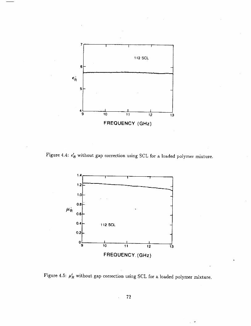
2.3.1 Measurements without Gap Corrections I
Various measurements have been made in waveguide and coaxial li~le. Some of the results of these measurements are reported i l l figures 2.3 througl~ 2.14 for the full S-parameter technique and in figures 2.15 and 2.16 for the two-sample length nlethod. The ~neasurements reported in this section are not corrected for gaps around the sample. 7yhe effect of the air gaps is to measure values of the material parameters that are lower than the actual values. In the next section we will discuss ways of mitigating the effects of air gaps.
2.3.2 Effects of Gaps between Sample and Waveguide
Gaps between the sample holder and sample either may be corrected with the formulas given in the appendix or a conducting paste can he applied to the external surfaces of the sample that are in contact with the salnple holcler before insertion into the sample holder. I11 figure 2.17 we show a measusenlent of a nickel-zinc ferrite with and without a gap-filling grease. The dielectric loss factor is increased slightly by the gap filling. We suspect that . part of this increase is due to the finite conductivity of the conducting grease.
Frequency (GHz)
Figure 2.4: r& of a loaded polymer in a X- band waveguide with the full S-parameter iterative techniqde.
1.500
1.375 .+-*- Nicolson-Ross
- Iterative
pR' 1.250
1.125
1.000 8.5 9.08 9.66 10.24 10.82 11.4
Frequency (GHz)
Figure 2.5: p k of a loaded polymer in a X-band waveguide with the full S-parameter iterative technique.
1 .oo 0.89
0.78 ***..- Nicolson-Ross
0.67 - Iterative
0.56
11;; 0.45
0.34
0.23
0.12
0.0 1
-0.1 8.4 9 9.6 10.2 10.8 11.4
Frequency (GHz) I
F1gi11.e 2.6: p i of a loaded polymer in a X-band waveguide with the full S-parameter i t e ~ a ~ i v e technique.
10 12 Frequency (GHz)
Figure 2.7: ck of a ferrite in a X-band waveguide with the full S-parameter iterative tech- nique.
10 12
Frequency (GHz)
Figure 2.9: / L ; ~ of s i t i n X-batld ivsveguidc wit11 f.hr f u l l S - l ~ a r a ~ n e t e r iterative technique.
Figure 2.8: cy3 (,I. fcrl.itr in a X-band wavrgi~ide wit11 t h e f r i l l S-paramrt.er iterative t,rl:h-
nique. 0.7 t
0.6 -
f 0.5 -- -
0.4 - cck -
0.3 - -
-
0.1
0
- -
I I I - 8 10 12 14
Frequency (GHz)
Frequency (GHz)
Figure 2.10: p i of a ferrite in a X-band waveguide with the full S-parameter iterative technique.
14
12
10
8 ~k
6
4
2
0 1 3 5 7 9 11 13 15 17
Frequency (GHz)
Figure 2.11: tk of a loaded polylner it1 coaxial line \sit11 the full S-parameter iterative technique.
Frequency (GHz)
Figure 2.12: e'fc of a loaded polynler in coaxial line the full S-parameter iterative technique.
4
3
1
0 1 3 5 7 9 11 13 15 17
Frequency (GHz) Figure 2.13: pk of a loaded polymer in coaxial line with the full S-parameter technique.
iterative
Frequency (GHz)
Figure 2.1-1: p$ of a loaded polymer in coaxial line with the full S-parameter iterative technique.
Frequency (GHz)
Figure 2.15: c;1 of a loaded polymer in a X-band waveguide with TR method for two sample technique, for three different samples.
Figure sample
Frequency (GHz)
2.16: ph of a loaded polymer in a X-band waveguide with TR technique, for three different samples.
1000
100
10
1
0.1
0.01
method for two
Frequency (GHz) Figure 2.17: The dielectric and magnetic parameters of a nickel-zinc ferrite in a coaxial line from 1 MHz to 10 GHz with the fill ~ -~ararne te r iterative technique.
2.4 Permeameter
In the past permeameters have been used for high permeability materials. Rasmussen [29], Hoer [30], Powell [31], and Goldfarb [32] have all described various permeameter setups. In this section we wish to review the theory behind the permeameter.
If a toroidal sample is inserted into an azimuthal magnetic field region, the inductance is changed. If the inductance of the empty sample holder is compared to the inductance of the filled holder then it is possible to extract the complex permeability of the material.
Consider a toroid of inner diameter a and outer diameter b and height h. The material contributes an inductance of [32]
and the inductance of the air space is
The net change in the sample inductance when the sample is inserted into the holder is
and therefore
The magnetic loss may be obtained from consideration of the core loss AR or resistance
These equations are a special case of the scattering equations for short-circuit line (see eq (4.7)) in the limit as w -, 0 and through use of relation Hd = E,/Z.
2.5 Uncertainty of Combined Permittivity and Per-
meability Determination
In this section an uncertainty analysis is presented. The sources of error in the permeability and permittivity T R measurement include
e Errors in measuring the magnitude and phase of the scattering parameters,
e Gaps between the sample and sample holder,
e Sample holder dimensional variations,
Uncertainty in sample length,
e Line losses and connector mismatch, and
Uncertainty in reference plane positions.
A technique for correcting errors arising from gaps arou~lcl the sample is given in Ap- pendix B [33,34,35]. Gaps betweell holder and sample either may be corrected using the formulas given in the appendix or conducting liquid solder call be painted on the external surfaces of the sample that are in contact with the sample holder before insertion into the sample holder, thereby minimizing gap problems. The formulas given in the literature gen- erally under-correct for the real part of the permittivity and over-correct for the imaginary part of the permittivity. We assume that all measurements of permittivity have been cor- rected for air gaps around the sample before the uncertainty analysis is applied. In order to evaluate the uncertainty introduced by the measured scattering parameters and sample dimensions, a differential uncertainty analysis is assumed applicable with the uncertainty due to Sll and Szl evaluated separately. We assume that the S-parameters are functions of S,,(ISlll, 1S211, 011, $21, L, d). We assume that the total uncertainty in th, where d is the air gap between the sample and waveguide. We assume that the uncertainties for the physically measured parameters are
where cr = 11 or 21, A0 is the uncertainty in the phase of the scattering parameter, AlS,l is the uncertainty in the magnitude of the scattering parameter, Ad is the uncertainty in the air gap around the sample, and AL is the uncertainty in the sample length. The derivatives with respect to air gap, de;l/dd, have been presented previously [26]. The uncertainties used for the S-parameters depend on the specific A N A used for the measurements. This type of uncertainty analysis assumes that changes in independent variables are sufficiently small so that a Taylor series expansion is valid. Of course there are many other uncertainty sources of lesser magnitude such as repeatability of connections and torquing of flange bolts. Estimates for these uncertainties could be added to the uncertainty budget.
2.5.1 One Sample at One Position
For the uncertainty analysis it is necessary to take implicit derivatives of the S-parameter equations with respect to the assumed independent parameters. It is assumed that the functions are analytic over the region of interest with respect to the differentiation variables. The independent variables are assumed to be IS2,[, lSlll, 021, and L. The derivatives of the S-parameter eqs (2.31) through (2.33) can be found analytically
asll az a€; az ap; as,, ar a€; sr sp; w[G@J I' Gm ' T[G + T - ] = O , dp, d(S2, I (2.70)
aszl az a€; az ap; as,, gr a€; ar all; +-y- +-,-]=O, E ' G ~ arR d l ~ l l I 1 + ~ ' ~ a ( s , , l dpR alslll (2.71)
as,, az a€; az ap;, as,, ar a€;, ar ap;, ---I ----- + ,-I + -[-- + ,----I = exp(jd2,) . (2.72) 82 a€;, a1szl I ailR als,~ 1 ar a€;, als,, I alsZ1 1
We can rewrite eq (2.69) - (2.72) as
where we have defined parameters A, B, C, and D. If we let
we can solve for the derivatives that have been taken with respect to the independent parameters in eqs (2.73)- (2.75):
c - B F - D E - d L B C - A D '
Figure 2.13: The derivative of c k by ISzl) vs L/X, with r;i = (5.0,0.02), pk = (2.0,0.03).
The measuremellt bounds for S-parameter data are ob tainecl from specifications for a network analyzer. The dominant uncertainty is in the phasc of SI1 as I Sll I---+ 0. The uncertainty in ISzl 1 is relatively constant until < -50 dB, when it increases abruptly. The various derivatives are plotted in figures 2.1 S through 2.27.
In figures 2.28 through 2.31 the total uncertainty in ck and 11; computed from Szl and SI1 is plotted as a function of normalized sa~llple length. For low-loss and high-loss materials a t 3 GHz with various values of ck and the guided wavelength in the material given by
In figures 2.28 through 2.31 the error due to the gap correction is not included, nor are there uncertainties included for connector repeatability or flange bolt torquing. The maximum uncertainty for low-loss materials occurs at multiples of one-half wavelength. Generally, we see a decrease in uncertainty as a function of increasing sample length. Also, the uncertainties in the S-parameters have some frequency dependence with higher frequencies having larger uncertainties in phase.
Figure 2.19: The derivative of E'R by 02i using S21 vs LIX, with e;i = (5.0,0.01), p;i = (2.0,0.03).
Figure 2.20: The derivative of c';1 with respect to 02i using S2, with = (5.0,0.01), p> = (2.0,0.03).
Figure 2.21: The derivative of c k with respect to L using Szl with c> = (5.0,0.01), pk = (2.0,0.03).
Figure 2.22: The derivative of 6; with respect to L using with r k = (5.0,0.01), pjl = (2.0,0.03).
Figure 2.23: The derivative of EL with respect to lSlll with c k = (5.0,0.01), p;1 = (2.0,0.03).
Figure 2.24: The derivative of c';, with respect to ISllI with ~ ; i = (5.0,0.01), p h = (2.0,0.03).
3 6
Figure 2.25: The derivative of c k with respect to ell using Sll with c R = (5.0,0.01), pR = (2.0,0.03).
Figure 2.26: The derivative of c$ with respect to ell using Sn with c k = (5.0,0.01), ~k = (2.0,0.03).
Figure 2.27: The derivative of EL with respect to L using Sll with ~ ; i = (5.0,0.01), p;i = (2.0,0.03).
Figure 2.28: The relative uncertainty in ~ k ( w ) for a low-loss material as a function of normalized length, with p;i = (2,0.05), EL = (10,0.05) and (5,0.05).
Figure 2.29: The relative uncertainty in &(w) for a low-loss material as a function of normalized length, with pj, = (2,0.05), &j, = (10,0.05) and (5,0.05).
Figure 2.30: The relative uncertainty in rk(w) for a high-loss material as a function of normalized length, with pk = (2,0.5), ck = (10,O.s) and (5,0.5).
3 9
Frequency (GHz)
Figure 2.31: The relative uncertainty in pk(w) for a high-loss material as a function of normalized length, with pk = (2.0,0.5), 6; = (10.0,0.5) and (5.0,0.5).
100
Figure 2.32: The real part of the relative permittivity E ~ ( w ) for a nickel-zinc compound with uncertainties.
10
\k,iby 1 I
0.001 0.01 0.1 1 10
Figure pound
Frequency (GHz) nickel-zinc 2.33: The imaginary part of the relative permittivity c'fi(w) for a
I
corn-
0.1
rrequenc (GHz) Figure 2.34: The real part of the re atlve perAeaolllty pk(w) for a nickel-zinc compound with uncertainties.
Figure 2.35: The imaginary part of the relative permeability p;h(w) for a nickel-zinc corn pound with uncertainties.
In figures 2.32 through 2.35 a measurement of a nickel-zinc ferrite compound is given with associated uncertainties. Uncertainties increase at high and low frequencies. At high and low frequency extremes the uncertainties in phase increase. Also, the scale is logarithmic which distorts the lengths of the error bars.
2.5.2 Two Samples of Differing Lengths
Another method to determine permittivity and permeability is the measurement of two samples with differing lengths. The advantage of this method is that each sample resonates at a different frequency and therefore Sll can be appreciable over the entire frequency band.
,We assume the S-parameters are fu~ctions of S,,(ISmnI, Om,, L1, L2). The parameters used for measurements on materials of low to medium loss are
since it is acceptable down to -40 dB. We assume that the lengths of the samples are L1 and L2 = aL1. Due to the two lengths, there are transmission coefficients for each sample
21 = exp(-yL1) , Z2 = exp(-ayLl) .
The relevant partial derivatives of eqs (2.97) are:
as21,2~ az2 a&: az2 aP: l+as21,2, ar a€: -[- +- ar a/43 ] = 0 , (2.101) T ' G ~ I ~ ~ ~ ( ~ ) I + G ~ I ~ ~ ~ ( ~ , I ar a~: als21(1,~ g;, als21cl)~
aS21(1) 321 a€;, 82, a p i aS21(1) dl? a€;, dl? I+-[- K [ G ~ I ~ ~ ~ ( ~ ~ I + % a ~ s ~ ~ ( ~ , ~ ar a&: ~ I S ~ ~ ( ~ ) I + G ~ I s ~ ~ ( ~ ) ~
1 = 0 , (2.102)
as,,,,, a 2 2 a€> 822 ] -I- a22 6% a l s 2 1 ( 2 , 1 + G a 1 s 2 1 , 2 , l as2l(,) ar a€;, ap;i +-[- ar at;, als,l(,)l + ~ a 1 s 2 1 , 2 , 1
1
We can rewrite eqs (2.100) through (2.103) as
as21,1, azl as,,,,, ar a ~ k -- +-- 1 ( az, arb ar a€;, als2,,,,l
where we have defined parameters A1, B1, A2, and B2. Also for the relevant derivatives with respect to length, we find
We now can solve for the derivatives that have been taken with respect to the indepen- dent parameters in eqs (2.104) through (2.107)
In figures 2.36 through 2.37, the total uncertainty in r k and p k computed from S2, is plotted as a function of normalized sample length, for low-loss and high-loss materials a t 3 GHz with various values of ck.
When the length of one sample is twice the length of the other sample, we see instability a t frequencies corresponding to nX,/2. Generally, we see a decrease in uncertainty as a
Figure 2.36: The relative uncertainty in C ~ ( W ) for a low-loss material as a function of normalized length for the case when L1 = 0.5 L2 for two different permittivities.
function of increasing sample length. Also, the uncertainties in the S-parameters show some frequency dependence. In figure 2.37 the ratio of sample lengths is a. In this case we see greater stability over the frequency range than in the case where the range is 0.5. Resonances in the solutions will occur when L = nXm/2 and crL = m X m / 2 simultaneously, where m is an integer.
Ad, - &R
Figure 2.37: The relative uncertainty in &(w) for a low-loss material a s . a function of normalized length for the case when Li = 2 L: for two different permittivities.
2.6 Uncertainty in Gap Correction
The correction for an air gap between the wall of the sample holder and sample is very a
important for measurements of high permittivity materials. In addition, the uncertainty
in the gap correction is very important for high permittivity materials and may actually dominant the uncertainties of the measurement. In appendix C the gap correction is worked out in detail. In this section the uncertainty in the gap correction will be worked out.
2.6.1 Dielectric Materials Waveguide Gap Uncertainty
The uncertainty due to an air gap between sample and holder can be calculated from the partial derivatives of with respect to sample thicknesses, d. The relevant derivatives for waveguide are given by
Coaxial Gap Correction
For coaxial line the relevant derivatives are given by
2.6.2 Magnetic Materials Waveguide G a p Uncer ta in ty
The uncertainty due to an air gap between sample and holder can be calculated from the partial derivatives of p i with respect to gap thicknesses, cl. The relevant derivatives for waveguide are given by
Coaxial G a p Correc t ion
For coaxial line the relevant derivatives are calculated using
as follows
2.6.3 Higher Order Modes The field model assumes a single mode of propagation in the sample. Propagation of higher ,
_ order modes becomes possible in inhomogeneous samples of high dielectric constant due to changes in cutoff. Air gaps also play an important role in mode conversion. Generally, the appearance of higher order modes manifests itself as a sudden dip in IS1,\. This dip is a result of resonance of the excited higher order mode. We can expect point-by-point
TR models to break down near higher order mode resonances for materials of high dielec- tric constant or inhomogeneous samples. Optimized, multi-frequency solution techniques fare better in this respect. The characteristic of the higher order modes are anomalies in the scattering matrix at and around resonance. Higher order modes require a coupling mechanism in order to begin propagating. In waveguide and coaxial line the asymmetry of the sample promotes higher order mode propagation. In order to minimize the effects of higher order modes, shorter samples can be used to maintain the electrical length less than one-half guided wavelength. Also well machined sample are important in suppressing modes. Higher order modes will not appear if the sample length is less than one-half guided wavelength of the fundamental mode in the material.
Mode Suppression
It is possible to remove some of the higher order modes by mode filters. This would be particularly helpful in cylindrical waveguide. One way to do this is to helically wind a fine wire about the inner surface of the waveguide sample holder, thus eliminating longitudinal currents and therefore TM modes. Another approach is to insert cuts in the waveguide walls to minimize current loops around the waveguide.
Chapter 3
Optimized Solution
3.1 Introduction
As indicated in the previous chapters, various numerical strategies have been employed for reducing 1-port and Zport scattering data for both nonmagnetic and magnetic materials. The vast majority of the work in this area has involved the determination of permittivity and permeability by the reduction of scattering data frequency by frequency, that is, by the explicit or implicit solution of a system of nonlinear scattering equations at each frequency (see [11,33]; as an example of a multifrequency approach see Maze et a1.[15]).
What is lacking in the literature are practical, robust, numerical reduction techniques for more accurate determination of permittivity and permeability in transmission lines. Reliable broadband permeability and permittivity results for low-lass, medium-to-high di- electric constant materials are hard to obtain with transmission line techniques. Coaxial line measurements are particularly hard to obtain due to air gap influences and overmod- ing. Traditional transmission line numerical techniques have difficulties to an extent that render these techniques of limited use for low-loss materials and for high dielectric constant materials. Difficulties arise with these methods for magnetic materials in that numerical singularities can occur at frequencies corresponding to integral multiples of one half wave- length. These instabilities arise from the fact that for low-loss materials both S21 and Sll become equations for the phase velocity, and the permittivity and permeability therefore enter as a product. These instabilities limit the acquisition of precise broadband dielec- tric and magnetic results in the neighborhood of a resonance. Another problem pertains to high dielectric constant materials. High dielectric constant materials are usually hard to measure since the theoretical models are limited to a single, fundamental mode and the data contain both fundamental and higher order mode responses. Further, point-by- point reduction techniques for magnetic materials contain large random uncertainties due
to the propagation of uncertainties through the equations. For nonmagnetic materials the propagation of errors is less of a problem.
In our search for better reduction techniques we have found that nonlinear optimization, which miriimizes the squared error, are a viable alternative solution. Optimization-based data reduction has an advantage over point-by-point schemes in that correlations are al- lowed between frequency measurements. In nonlinear regression, if deemed appropriate, it is not necessary to even include Sll data in the constraint equations. Another advantage of regression is that constraints such as causality and positivity can he incorporated into the solution.
This chapter presents a method for obtaining complex permittivity and permeahility spectra from scattering parameter data on isotropic, I~omogeneous materials using nonlin- ear regression. We solve the scattering'equations in a nodinear least-squares sense with a regression algorithm over the entire frequency measurement range. The complex per- mittivity and permeability are obtained by determining estinlates for the coefficients of a truncated Laurent series expansion for these parameters consistent with linearity and causality constraints. The procedure has been successfully used for accurate permittivity and permeability characteriza.tion of a ~lulnber of different samples where point-by-point schemes have proven to be inadequate. The details of the numerical method have been presented in [36]. The problem applied to l~licrowave measurements is presented in this chapter. The method can easily be extended to the analysis of multi-mode problems and the determination of experimental systematic. rrt~cc.~.tair~t,y. Tlie novel features o f our algorithm are:
The algorithm finds a "hest lit" to t l ~ e ;'-port scattesil~g ecluatiolis using a nonlinear least-squares solution for the pernlittivity and ~)ernieability.
The algorithm uses fitting functions that satisfy causality requirements.
o The numerical technique allows slight vaxiations in the sample a.11~1 reference position lengths to compensate for ~neasuremcnt errors ant1 saml>le impesfections.
0 The method allows the cle-emphasis of f~.e<~rlc~~cy ~)oillts wit11 large phase u:lcertainty.
o Statistics related to the soliltion parameters arc autonta tica.lly generated.
o The technique can force positivity of the fit functions.
0 It is possible to deterrni~~e both complex pertnittivit.y a l ~ d permeahility from measure- ~ r ~ e n t s of a single scattering paranteter oli a. I-port or a 2-port taken over a frequency hand.
3.2 Model for Permeability and Permittivity In the optimization procedure the S-parameter eqs (2.31) through (2.33) for single-mode problems, or eqs (2.21) through (2.24) for prohlems with higher order modes are solved for the material parameters by the optimization routine. For higher order mode problems the matrix elements AJk in eqs (2.21) through (2.24), which corresponds to the voltagc; in each mode, can be determined by the optimization routine. However, we usually consider only the primary mode.
The unknown quantities are L1, L2 , L, A,, and pk(w) and +(w). Some of these parame- ters, such as the lengths and cutoff wavelength, are known accurately within measurement uncertainty. Obviously the parameters of interest cannot be allowed to vary into non- physical realms. The problem is to use an optimization routine to determine the model parameters that are consistent with the scattering clata and the physics of the problem.
3.2.1 Relaxation Phenomena in the Complex Plane
The numerical model requires all explicit functional form for p>al~d c;; to reproduce the four S-parameters consistent with the data, for all the 17, frequency observations.
The general form for pk(w) and ~ ; i ( d ) sl~ould be causal see Appendix C; that is, it must satisfy a Kramers-I<ronig relation. If the zeros and poles of a complex function are known over the complex plane, the f~inctiori itself is known.
The Laplace transform of the real, time-dependent perlnittivity satisfies
For stability, there can be no poles in the right-half side of tlie s-plane. Since ~ ( t ) is real it can be shown that the poles and zeros are confined to the negative real s-axis of the s-plane, and the poles which are off the real s- axis must occur in complex conjugate pairs
[371. Assuming linear response a constitutive relationship in a n isotropic medium between
the displacement and electric fields is
-, 'X,
d ( ? , t ) = t , ~ ( i , i ) + c , ~ G ( T ) E ( . F . L - T ) ( ~ T . (3.2)
With this defil~itiol~ tlie perlriit t,ivit,y is
The response function G ( T ) for an incident electric field can sometin~es be represented as a series of damped sinusoids of the form
We assume that the material parameters can be adequately modeled by a series of sim- ple poles. The terms e-""' relate to relaxation and the terms e-3bnt relate to resonant phenomena. Since the Laplace transform of eq (3.4) is
for stability (no increasing time domain exponentials) there can be no poles or zeros in the right half-side of the s-plane [37], [35]. In order to maintain the reality of ~ ( s ) , any poles off the imaginary axis in the w-plane must be conjugate poles of the form w = ja f b where a and b are real, positive numbers as indicated in figure 3.1. These conjugate poles are of the form
1 1 + s + a + j b s + a - j b ' (3.6)
and are related to resonant phenomena. We assume that the permittivity can be expressed as
( j w + 5,) + zr 1 + I].
( j w + p , ) , ju + a, + jb, jw + ( 1 , ~ - jb,
Here z, and p, are the zeros and poles clue to damped expo1~1entia.1~ respectively, ( a , f jb,) are the complex conjugate poles, and C is a complex constant.
Figure 3.1: Poles (X) and zeros (0 ) i l l tlie complex s-plane a~lcl conjugate poles off the real s-axis.
For more complicated polarization phenomena other relations for permittivity could be used. For a continuous distribution of relaxation times
where Y ( T ) is a distribution function. Various expressions for y yield various relations for permittivity. Presently we use eqs (3.11) and (3.12) in our calculations. The Havriliak- Negarni model for materials assumes a single nonsimple pole on the negative, real sp lane axis:
where ,L? and cr are in the it~tcrval [O, I ] and B is real. IJilt~itillg cases of this model are (1) the Cole-Davidson model when a = 0; this ~notlel works well for some liquids and solid polymers, (2) the Cole-Cole model when /? = 1; this motlel has been used to describe relaxation behavior of amorphous solids ancl many liquitls. A simple Debye model ( P = 1 and a = 1) is very limited and works well only for materials that c o n t a i ~ ~ a single relaxation time in the frequency range of interest.
Heterogeneous materials and polymers usually have a very broad relaxation spectrum and as such have a response of the for~n of a power law silcli as S - " . This behavior can be obtained from the Cole-Davidson model wheli lBlw >> 1 .
8
In our present algorithm we assulne a more general model tlian the single Debye relax- ation model a truncated Laurent series is used for J L + R ( w ) and cR(w). This expansion has
generally yielded excellent results
where B; are real numbers. The pole information yields constraints on the constants used in the Laurent series expansion. For example, it is required that B; is a real number.
For a typical measurement on a network analyzer there may be 400 frequency points and at each point all four scattering parameters are taken. The problem is overdetermined since for n frequency measurements, if we assume known lengths, there are 8n real equations for th6 unknown quantities in the Laurent series. This over determination can be used at frequencies in the gigahertz range to find corrections to sample position and cut off wavelength.
The approach for determining the complex parameters A,, Bj is to minimize the sum of the squares of the differences between the predicted and observed S-parameters,
rnin 11 C3;, - R j 11 , . . '3
where the measured vectors are denoted by Sjj = (Si,(wl), Si,(w2), .., S,(w,)) and where gj is the predicted vector. Hence, the problem consists of finding the norm solution to these e4uations.
3.3 Numerical Technique
3.3.1 Algorithm
The solution currently uses a software routine called orthogonal distance regression ~ a c k ODRPACK [39] developed at the National Institute of Standards and Technology. This routine is an extended form of the Levenberg-Marquardt approach. This procedure allows for both ordinary nonlillear least-squares, in which the uncertainties are assumed to be only in the dependent variable, and, orthogonal distance regression, where the uncertain- ties appear in both dependent and independent variables. First-order derivatives for the Jacobian matrices can be ay~>roxi~natecl (finite tlifference approximation) or can be user-supplied analytical derivatives. The procedure performs automatic scaling of the variables if necessary, as well as determining the accuracy of the model in terms of ma- chine precision. The trust region approach enables the procedure t~ adaptively determine the region in which the linear approximatio~l adequately represents the nonlinear model.
Iterations are stopped by ODRPACK when any one of three criteria are met. These are: (1) the difference between observed and predicted values is small, (2) the
convergence to a predicted value is sufficiently small, and (3) a specified limit on the number of iterations has been reached.
Initial guesses for ch and pk are obtained from explicit solutions of Stuchly [7] or Weir [6]. The most significant input parameters for modeling permittivity and permeability are the initial values for A; and B;. Sensitivity to the initial solution for these parameters is discussed below. All additional parameters are initialized to 0.
When measurements of length and scattering parameters of a sample are taken, there are systematic uncertainties.
An orthogonal distance regression model provides the modeler with the additional abil- ity to assume that the independent variable, in this case, frequency, may contain some uncertainty as well. Allowances for these types of uncertainty can, in some cases, greatly improve the approximation. For this model and the samples tested, the errors in the in- dependent variables are sufficiently small that an ordinary least-squares approximation is adequate.
Model parameters such as sample length, sample position in the waveguide, and cutoff wavelength could contain a systematic uncertainty. These parameters were allowed to vary over a limited region, and the optimization procedure chooses optimum values for the parameter. This procedure assumes Lhat systematic measurement errors can be detected by the routine. For example, inserting a sample into a sample holder introduces an uncertainty in the sample position L1, so we include with L1 an additional optimization parameter PL1 in R1 to account for positioning uncertainties,
Also for B2 R2 = exp(-"~o[L2 + P L ~ ] )
The routine requires that the length corrections be within a prescribed range which repre- sents physical measurement uncertainty. The length of the sample L is completely deter- mined by
L = La;, - (L1 + Lz + PLI + P L ~ ) (3.16)
and is also implicitly parameterized by the values of PL1 and PL2. Due to inaccuracies in machining of the sample holder there is an uncertainty in the
cutoff wavelength of the guide. We account for this by the introduction of an additional optimization parameter A , --+ A,+P,\. We constrain this variation to be within measurement accuracy.
The model can use various combinations of the available data to estimate both the relative permeability and permittivity from scattering data. For example, Szl or Sll alone
Frequency (GHz) Frequency (GHz)
Figure 3.2: Predicted (solid line) and observed (dots) parameters for a barium titanate compound (a) and cross-linked polystyrene in (b).
can be used to obtain both permeability and permittivity. This can be contrasted with point-by-point techniques where both and Sll are required. Also, magnitude alone can similarly be used. Magnitude data have the advantage of requiring no reference plane rotation.
The technique works well for short-circuit line measurements. For short-circuit lines it is possible with this technique to obtain both the complex permittivity and permeability
, from a single broadband measurement on one sample at a single position in the line.
3.3.2 Numerical Results The model predictions are formed by inserting eqs(3.11) and (3.12) into (2.31) and (2.33) or (4.7) and then finding the unknown coefficients in the ecluations for ek and pk that produces the least square error. In figure 3.2 the experimental results are given for a barium titanate compound and cross-linked polystyrene. These samples required 21 and 40 iterations respectively.
The difference between the predicted S-parameter and the observed values reveals the presence of systematic uncertainty, as shown in figure 3.3, in the automatic network analyzer (ANA). Additional tests revealed the source of the systematic error did not appear to be related to the material tested in the waveguide. In fact, uncertainties produced for the cross- linked polystyrene sample closely resemble the S-parameter data for an empty waveguide;
0 002 h
C ,- 0.0 - m
d -0.002
-0.004 8 9 10 11 12 13
Frequency (GHz) (a)
Figure 3.3: Systematic uncertainty as indicated by the residual plot (the difference between the observed and predicted values) for the case on an empty waveguide. The solid line is at 0 residual.
we conclude therefore that much of the systematic error is due to calibration uncertainty and joint losses at connector interfaces. For the barium titanate compound sample there is both the fundamental mode response and smaller resonances related to higher-order modes. As shown in figure C.l, the model interpolates a fundamental mode. This raises the possibility of extending the model to incorporate higher-order modes by extending the theoretical formulation of the problem.
It is easy to move the sample in the holder inadvertently when connecting the sample holder to the port cables. Positioning errors of the sample in the air line can result in large error in computed material parameters. The numerical algorithm can adjust for positioning errors by adjusting L1 or L2 slightly. The effects of positioning error can be seen in figure 3.4.
In this example the routine predicted that the position of the sample was off by 0.8 mm.
Frequency (GHz) (a)
Frequency (GHzf (b)
Figure 3.4: Measured real part of Sll, measured (. . . . ) and predicted (------- 1, for a glass sample (a) with positioning error for L1 and (b) the solution when the algorithm adjusts for the positioning error.
3 .4 Permittivity and Permeability
3.4.1 Measurements
In this section we present the measured and calculated permittivity and permeability. Cross-linked polystyrene and the barium titanate compound are nonmagnetic and therefore p;i = 1. Comparison of the optimized solution to a point-by-point solution is shown in figure 3.5. In figures 3.6 through 3.9 results for four samples are given.
As a check we ma.de an independent measurement of the barium titanate compound in an X-band cavity where the results were EL = 269 at 10 Ghz. This result can be compared to the results in figure 3.6. Finally a result of another bariu~ll titanate compound is given below.
3.4.2 Robustness of the Procedure
Since the transmission coefficient contains a periodic component, there is more than one solution to the system of equations. Each soot of the ecluation has a neighborhood around which convergence will occur for iuitial guesses in that region. 'rhe robustness of a mathe- matical procedure is relatecl to how well the algorithm treats the neighborhood around the
Figure 3.5: Permittivity in the frequency ra&e of 0.045 - 18 Ghz for the optimized solution (- - - - ) and point-by-point technique (-).
Figure 3.7: Permittivity and permeability for a loaded-polymer, point-by-point method (. . . .) , optimized solution (--).
Frequency (GHz)
Figure 3.8: Real part of permittivity for a barium titanate compound (0 0 0) cavity (. . .) optimized solution.
Frequency (GHz)
Figure 3.9: Imaginary part of permittivity for a barium titanate compound o o o -cavity and . . . - optimized solution.
correct root. The existence of alternative optima in the mathematical model requires an accurate initial guess in order to converge to the correct solution. Typically convergence occurs after about seven iterations. The use of constraints and the large number of equa- tions enhances the uniqueness of the solution by reducing the dimensions of the solution space.
In point-by-point methods the correct solution is selected from the infinity of possible roots by calculating the slope of the phase curve and comparing the measired and calculated group delays. A group delay constraint is also used as a way of determining the physical solution.
The numerical effectiveness of the entire permeability and permittivity calculation de- pends on the robustness of the ODRPACK procedure and, more significantly, the robustness of the mathematical model. For the samples used in this study, the robustness of the proce- dure depended on the sample. For the materials with low dielectric constant the procedure readily determined a solution for a variety of input values with a large radius of conver- gence. For materials with higher dielectric constant, the procedure often converged quickly, although the existence of alternative local optima in the mathematical model required some , testing to make sure that the converged root was the correct root.
3.5 Discussion
An optimization approach to the solution of the scattering equations appears to be a viable alternative to point-by-point techniques. The technique allows a stable solution for a broad range of frequencies. The method works particularly well for short-circuit line measure- ments. Unlike the point-by-point short-circuit method which requires measurements on two samples or in two positions, the optimized solution can obtain complex permittivity and permeability on a single sample at a single position.
The reflection (Sll) data are usually of lesser quality than the transmission data (S21) for low-loss, low- permittivity materials. Therefore Sll need not be included in the solution for low-loss materials. However, reflection data Sll and S22 are very useful in determining the position of the sample in the air line as indicated in figure 3.7. The technique was successful for many isotropic magnetic and relatively high dielectric const ant materials. The addition of constraints to the solution is powerful in that it further limits the possible solution range of the system of equations and enhances the uniqueness of the solution. The use of analytic functions for the expansion functions allows a correlation between the real and imaginary parts of the permittivity and permeability. The results shown in figures 3.5 through 3.6 indicate that the method can be used to reduce scattering data of fairly high dielectric constant materials. In fact, in some cases the optimized procedure yields solutions when the point-by-point technique fails completely.
Why does an optimization approach, in many cases, reliably reduce data on higher dielectric constant materials ( r h > 20), whereas point-by-point techniques generally fail? Scattering data for higher dielectric constant materials contain responses to both primary mode and higher order modes. As indicated in figure 3.2 for the barium titanate compound, the optimization routine selects the primary mode data and places less weight on the higher mode resonance data.
The optimized technique can be used to treat problems where sample lengths, sample holder lengths, and sample positions are not known to high accuracy. Permittivity and permeability can be found from the equations without specifying either sample position or sample length. This result could find application to high-temperature measurements.
Higher-order modes propagate in samples when two conditions are met. The frequencies must be above cutoff in the sample, and there must be inhomogeneities or asymmetries in the sample to excite the higher order modes. Higher-order modes can be incorporated into this type of model by letting the optimization routine select the power in each mode. Higher-order mode models are a subject of our current research.
Chapter 4
Short-Circuit Line Met hods
4.1 Theory
In this section we review the mathematical formalism for short-circuit measurements. We consider a measurement of the reflection coefficient (Sll for a shorted two-port) as a function of frequency. We begin with a mathematical analysis of the electromagnetic fields in the sample. The details of the field model have been presented previously [26] and only the most essential details will be presented here.
Assumptions on the electric fields in regions I, 11, and I11 shown in figure 4.1 may be made as follows: (1) only the dominant mode is present in the waveguide; (2) the materials are homogeneous and isotropic; (3) only transverse electric fields are present. Under these conditions the electric fields in these regions may be expressed as:
EI I I = C4 exp(-yo(-. - L ) ) + Cs exp(yo(z - L)) . (4.3)
We wish to determine the coefficients in eqs (4.1) through (4.3) by imposing boundary conditions on the system of equations. The boundary conditions are:
0 Tangential component of the electric field is continuous at sample interfaces.
e Tangential component of the magnetic field is continuous at sample interfaces.
0 The electric field is null at the short-circuit position (perfect reflect).
Figure 4.1 : A transmission line with a short-circuit termination.
Expressions for the coefficients in eqs (4 .1 ) through (4 .3) are presented in reference [26]. Matching boundary conditions of the field equations at the interface and the reflect
yields an equation for the permittivity and permeability in terms of the reflection coefficient, p = Sll = C1. With the sample end face located a distance A L from the short,
Sll = p = -2P6 + [ ( 6 + 1) + (S - 1 ) P 2 ] tanh y L
2P + [(6 + 1) - ( 6 - l ) p 2 ] tanh y L ' (4.4)
where
and 5 = exp(-2y,AL) .
In terms of hyperbolic functions
tanh y L + ,f3 tanh yoAL - p ( l + P tanh y L tanh 7 o A L ) Sll = tanh y L + ,B tanh yoAL + P(l + P tanh y L tanh Y o A L ) ' (4.7)
311 for a matched two-port can be obtained as a special case from ecl (4 .4 ) by letting 6 4 0. Although in the derivation of eq (4.7) it is assumed that the sample plane coincides
with the measurement calibration plane, this is not the case in general; however, we call transform the reference plane position by a simple procedure. To accomplish this, we write the most general expression for the reflection coefficient as
Sll(trans) = R:Sll , (4.8)
where SII,a,, is the reflection coefficient at the calibration reference plane position,
and L1 is the distance from the calibration plane to the sample front face. Equation (4.8) transforms the reflection coefficient from the calibration plane to the plane of sample front face. It is of interest in many applications to eliminate the distance L1 from eq (4.8). This can be accomplished by measuring Sll of the empty sample holder,
Sll(,mPtv) = -exp(-2%[Ll + AL + L ] ) = - exp(-2yoLnir) , (4.10)
and therefore the ratio of the filled to empty holder reflection coefficient is
If both the permeability and the permittivity are required, measurement data for two different short-circuit positions are needed. Note that standing waves can be formed in the region between the sample and short-circuit and between the calibration plane and sample front-face. Therefore certain frequencies, depending on sample length and the other lengths, will give better results for permittivity and other frequencies better results for permeability.
The position of the short-circuit is a low electric field and high magnetic field region and a position X/4 from the short- circuit is a high electric field and low magnetic field region. Therefore as frequency permits, for permittivity measurements the sample should be moved away from the short-circuit termination- Permeability in isolation can be obtained with the sample at the short-circuit position. Of course when an A N A is used measurements will be taken a t many combinations of field strengths ancl therefore the uncertainty will vary with frequency.
4.1.1 Two Samples of Different Lengths
It is possible to solve for the permeability and permittivity when the scattering parameters with samples of two differing lengths are measured. To see this, let us consider two samples, one of length L and one of length aL as indicated in figure 4.2.
Then for independent measurements on the two samples we have .
and
Figure 4.2: A transmission line with a short-circuit termination in two sample magnetic measurements.
The reflection coefficient I' is given by eq (2.37). The scattering 1-port parameter is given by
Therefore we can solve for Z in eq (4.12),
and substitute it into eq (4.14) to obtain
Equation (4.16) is solved iteratively for r and then Z is found from eq (4.15). The permit- tivity and permeability can then be obtained, if we define
Port 1 I
2 Short-Circuit
Position 2 Position I
Figure 4.3: A transmission line with a short-circuit termination for two-position measure- ments.
where A,, is the free-space wavelength and A, is the cutoff wavelength. Equation (4.17) has an infinite number of roots for magnetic materials because the logarithm of a complex number is multi-valued. In order to pick out the'correct root it is necessary to compare the measured to the calculated group delay.
4.1.2 Single Sample at Two S hort-Circuit Positions
It is possible to obtain an explicit solution to eq (4.4) when measurements a t two different short-circuit positions are taken. The explicit solution is obtained by solving eq (4.4) at a given short-circuit position (position 1 ) for tanh y L and then substituting this expression into eq (4.4) at another short-circuit position (position 2) as indicated in figure 4.3. +
For two different short-circuit positions at the same frequency we obtain pl and p2 for positions 1 and 2:
where 61,b2 denote the phases calculated from eq (4.6) for AL1, AL2 respectively. These equations yield
tanh y L = 2P(61 + Pl) P2(p1 t 1)(61 - 1) + (1 - p1)(61 + 1) '
where n is an integer. Since the arctangent is multi-valued, the correct value of n is determined from the group delay arguments given in section 3.2.1. Also
Once ,8 is know'n, eqs(4.22) and (4.24) can be used to find permittivity and permeability.
4.2 Measurements
In the SCL technique the scattering parameter Sll is measured broadband, with the sample a t a given position in the sample holder. The distance from the sample to the short-circuit termination must be known to a high degree of accuracy. If both permeability and the permittivity are required then the sample must be moved in the line and the S-parameters again taken.
Depending on the position of the short-circuit, the sample may be immersed in either a region of high electric field or high magnetic field. A strong electric field is advantageous for permittivity determination, whereas a strong magnetic field is advantageous for ~ermeabil- ity determination. Generally, the sample end will be in a region of high magnetic field when the sample is in closest physical contact with the short. It is possible to take advantage of the flf-ctuating electric and magnetic field distributions when performing permittivity and permeability measurements. When taking broadband measurements on an ANA it is possible to predict when the sample is immersed in the various field strengths. Then one can select the measurements to be used for permittivity and permeability calculations [35].
Measurements were made on an ANA for various samples. Using eq (4.4) we obtain the permittivity and permeability which are shown in figures 4.4 and 4.5.
I 112 SCL
FREQUENCY (GHz)
Figure 4.4: s k without gap correction using SCL for a loaded polymer mixture.
FREQUENCY. (GHz)
Figure 4.5: pk without gap correction using SCL for a loaded polymer mixture.
72
For magnetic materials it is necessary to make two independent measurements at a given frequency. Independent measurements can be obtained either by measuring samples of two different lengths or by taking measurements of a given sample at two locations in the line. The special case of measurement of two samples of varying lengths (L1, L2) can be obtained from the solution presented below by substituting L 4 L1, yo 4 y and AL + L2 - L1.
The uncertainty involved in two position measurements is explored in this section. The uncertainty incurred with the equations expounded in this report is estimated. The sources of uncertainty in the SCL measurement include
e Uncertainties in measurements of-the magnitude and phase of the scattering param- eters.
e Gaps between the sample and sample holder.
e Dimensional variations in the sample holder.
Uncertainty in sample length.
e Short-circuit and line losses and connector mismatch.
e Uncertainty in positions of the reference plane and sample in holder.
Adjustment for errors due to gaps around the sample is obtained from equations avail- able in the literature [33,34,35]. The formulas given in the literature generally under-correct for the real part of the permittivity and over-correct for the imaginary part of the permit- tivity. All measurements of permittivity are assumed to have been corrected for air gaps around the sample before the following uncertainty analysis is applied.
In order to evaluate the uncertainty introduced by the measured scattering parameters, we assume that a differential uncertainty analysis is applicable. This assumption implies that uncertainties are of small enough magnitude so that a local Taylor series can be applied. We assume that a Taylor series approximates deviations of the function from a given point. We assume that the worst case uncertainty due to the S-parameters and sample lengths can be written
where A9 is the uncertainty in the phase of the scattering parameter, AlS,,] is the un- certainty in the magnitude of the scattering parameter, Ad is the uncertainty in the air gap around the sample, and AL is the uncertainty in the sample length. The gap correc- tion uncertainty is given in [26]. The uncertainties used for the S-parameters depend on the specific ANA used for the measurements. In general uncertainties due to flange bolt torquing and connector repeatability must be added to these uncertainties.
Let us define the variables
b = tanh yoAL . (4.28)
We wish to obtain explicit relations for the derivatives of ~ ; i and p;i with respect to inde- pendent variables lSll(;l 1 and 8;, i = 1,2. We define S1l(l) as the reflection a t short position 1 and S11(2) as the reflection at short position 2. Next define
tanh yL + p tanh yoAL - /?(I+ p tanh yL tanh yoAL) - s,, = 0 . = tanh yL + p tanhyoAL + p(1 + p tanh yL tanh yoAL)
(4.29)
We assume the following as independent variables Sll (i), i = 1,2, L, AL, and d. Derivatives of eq (4.29) with respect to the independent variables can be found analytically. By the chain rule we have
a f aa a f aa; --- 8 f da dy + -- --- +-- a f a p I a€; [aa ay apk a p ap;, ajsll (m) 1 + ',a By a ~ h aP a€;, al sll (m) 1 = exp(j8,) , (4.30)
* + 01 a2
This equation is evaluated a t position one.
This equation is evaluated at position two. The four derivatives can be written
where S;,, is the Kronecker delta function.
At the first position the derivatives with respect to length are
and for the second short-circuit termination position
The derivatives with respect to the distance from the sample bacli face to the short-circuit termination can similarly be calculated
af a a a7 af ap a,; af aa af aa a p k a j db + -- 1,- + [--- + --: - +--=o [a&% apapk ~ A L a a a 7 a t ; d / 3 d r R r n d ~ ~ a b a ~ ~ , (4.37)
and for the second short-circuit position
The derivatives can be calculated explicitly to yield
af - - - da
1 - p2 tanh yoAL
t a n h ~ L + PtanhyoAL + P(l + ~ t a n h y ~ t a n h y ~ ~ L ) - tanhyL +ptanhyoAL + P( l + Ptanh yLtanhyoL)
( tanhyL + Ptanh yoAL + P(l + P tanh yL tanh yoAL)2 X
(1 + P2 tanh ~ O A L ) ,
af - - - d b
p - P2tanhyL
tanh yL + B tanh yoAL + P(1 + j? tanh yL tanh -
tanhyL + Ptanh yoAL + P(1 + P tanh yL tanhyoL) X
(tanh +/L + P tanh yoAL - p ( l + P tanh yL tanh +L)2 ( P + P2 tanh yL) , (4.41)
- tanh yL + /3 tanhyoAL + P ( l + P tanh yL tanh yoL) X
(tanh y L + ,6 tanh yoAL - P(1+ ,6 tanh y L tanh ~ o A L ) ~
(tanh yoAL + 1 + 2P tanh yL tanh yoA L) .
The following derivatives will be needed in the forthcoming analysis
Figure 4.6: A plot of the derivative of EL with respect to ISll 1 as a function of the distance from the short-circuit termination for the case of thin samples L << A,.
In figures 4.6 and 4.7 8c>/alSllI is plotted as a function of the distance from the short circuit termination. We see that in the case of electrically thin samples the minimum uncertainty occurs when the second sample measurement is at Xo/4 from the short-circuit termination. As shown in figure 4.7, this is not the case for samples that are not electrically thin.
Figure 4.7: A plot of the derivative of with respect to ISl1\ as a function of the distance from the short-circuit termination for the case of long samples L x A,.
Chapter 5
Discussion a
we' have presented an overview of the theory and the measurements for both the TR method and the SCL method for dielectric and magnetic materials. In addition, relevant uncertainty analyses have been developed. Equations were presented for TR and SCL measurements that are reference plane invariant. These equations can be solved either by iteration or explicitly.
There are two common problems in the data reduction techniques for transmission line measurements. These problems are the existence of higher mode resonances and the problem that for low- loss materials the solution of the equations become ill-conditioned at integral multiples of one-half wavelength in the sample. The one-half wavelength instability occurs because the phase of SI1 contains a large uncertainty when (SI11 -, 0 and also because the equations in this limit yield only the phase velocity. For dielectric and magnetic measurements, the uncertainty is a function of the sample length. In general for low- loss materials, samples long in relation to wavelength give more accurate results, however overmodes may be produced. Thus for broadband measurements of low-loss low- dielectric materials, it is preferable to use longer samples. However, with lossy materials, very long samples result in only front face reflection information and the results have a relatively large uncertainty. For relatively lossy materials, sample lengths on the order of one attenuation length are optimum. Longer samples allow the propagation of higher order modes, and therefore higher mode responses will be contained in measured scattering data. However, the uncertainty in the spectrum between over-moded resonance regions will be lower for longer samples than for electrically short samples.
For thicker samples the problem is more complicated and a knowledge of the uncertainty analysis is important for interpreting the results. For permeability measurements in a short- circuit line the numerical reduction procedure becomes divergent when there is an integral multiple of one-half wavelength in the sample. For TR and SCL measurements we can summarize our conclusions as follows
For SCL measurements, length of samples should be such that ISI1I > -20 dB.
The one-sample techniques appear to allow a better reduction of the scattering data.
The optimized solution and the reference plane invariant solution appear to be the most accurate and stable methods. However, local minima have to be avoided.
0 The short-circuit line is a simple way to obtain permittivity and permeability simul- taneously. For low-loss materials it does suffer from numerical instabilities.
In SCL permittivity measurements, minimum uncertainty is obtained when the sam- ple is X/4 from the short. This is only true for electrically thin samples.
o Minimum uncertainty magnetic measurements can be made for single frequency mea- surements by taking one measurement at a maximum electric field position and an- other measurement at a maximum magnetic field position.
The various TR and SCL techniques are compared in table 5.1 and 5.2.
Table 5.1: Dielectric and magnetic TR measurement techniques compared.
Multi-point techniques Magnetic Very stable non-global minima
Table 5.2: Dielectric and magnetic SCL measurement techniques compared.
Weak Points ' -
Unstable a t nXm/2
Requires two samples
Alternative minima
Technique One-posit ion Technique
Two.Position Technique
T w o sample technique
Multi-point techniques
Applicability Dielectr~c
Magnetic
Magnetic
Magnetic
Strong Points Stable
Requires only one sample
Stable over all frequencies
Very stable
m'e would like to thank Eleanor Livingston for her excellent comments and sugges- tions, Paul Domich for collaboration on the optimized solution, Chris Jones for help with measurements and plotting, William Kissick, Claude Weil, and Howard Bussey for various discussions and as sources of encouragement. Finally we would like to thank Ramon Jesch, Bill Daywitt, and Lydell Frasch for reviewing the manuscript.
References
[l] Belhadj-Tahar, N.; Fourrier-Lamer, A.; and de Chanterac, H., "Broadband simulta- neous measurement of complex permittivity and permeability using a coaxial discon- tinuity," IEEE Trans. Microwave Theory Tech., vol. 2, pp. 1-7, January 1990.
[2] Deschamps, G. A., "Determination of reflection coefficients and insertion loss of a wave-guide junction," J. A p p l . Phys., vol. 2, pp. 1046-1050, August 1953.
[3] "Measuring dielectric constant with the HP 8510 network analyzer," Product note no. 8510-3, Hewlett Packard, 1985.
[4] Freeman, M. S.; Nottenl,urg, It . N.; and DuBow, J. B.. "An automated frequency domain technique for dielectric spectroscopy of materials," J. Phys. E: Sci. Instrum., vol. 12, pp. 899-903, 1979.
15) Nicolson, A. M.; and Ross, G. F., "Measurement of the intrinsic properties of materials by time domain techniques," IEEE Trans. Instrum. Meas., vol. IM-19, pp. 377-382, November 1970.
(61 Weir, W. B., "Automatic measurement of complex dielectric constant and permeability a t microwave frequencies," Proc. IEEE, vol. 62, pp. 33-36, January 1974.
[7] Stuchly, S.; and Matuszewski, M., "A combined total reflection transmission method in application to dielectric spectroscopy," IEEE Trans. Instrum. Meas., vol. IM-27, pp. 285-288, September 1978.
[8] Delecki, 2. A.; and Stuchly, S. S., kcuncertainties in the determination of dielectric properties in the infinite sample method," IEEE Trans. Instrum. Meas., vol. .38, pp. 902-906, June 1989.
[g] F'ranceschetti, G., "A complete analysis of the reflection and transmission methods for measuring the complex permeability a ~ i d permittivity of tr~atel*ials at microwave," A h Freguenzia, vol. 36, pp. 757-764, August 1967.
1101 Ligthardt, L. P., "A fast computational technique for accurate permittivity deter- mination using transmission line methods," IEEE Trans. Microwave Theory Tech., vol. MTT-31, pp. 249-254, March 1983.
[ I 11 Roberts, S.; and von Hippel, A., "A new method for measuring dielectric constant and loss in the range of centimeter waves," J . Appl. Plzys., vol. 7, pp. 610-616, July 1946.
[12] Brydon, G. M.; and Hepplestone, D. J., "Microwave measurements of permittivity and tan 6 over the temperature range 20 - 700°C," Proc. Inst. Elec. Eng., vol. 112, pp. 421-425, 1965.
[13] Szendrenyi, B. B.; Kazi, I<.; and Mojzes, I., "An alternative broadband method for automatic measurement of the complex permeability and permittivity of materials a t microwave frequencies," Mici.owave Theory and Tech. Digest, vol. 1, no. 1, pp. 743-745, 1988.
[14] Mattar, K. E.; and Brodwin, M. E., "A variable frequency method for wide-band microwave material characterization," IEEE Trans. Instrum. Meas., vol. 39, pp. 609- 614, August 1990.
[15] Maze, G.; Bonnefoy, J. L.; and Icamarei, M., "Microwave measurement of the dielectric constant using a sliding short-circuited waveguide method," Microwave J., pp. 77- -88, October 1990.
[16] Dakin, T. W.; and Works, C. N., "Microwave dielectric measurements," J. Appd. Phys., vol. 18, pp. 789-796, September 1947.
[17] Bowie, D. M. and Kelleher, Ii. S., "Rapid measurement of dielectric constant and loss tangent," IEE Trans. Microwave Theory Tech., vol. MTT-4, pp. 137-140, 1956. -
[18] Sequeira, H. B., "Extracting p, and t, from one- port phasor network analyzer mea- surements," IEEE Trans. Inst?-urn. Meas., vol. 39, pp. 621-627, August 1990.
[19] Chao, S., "An uncertainty analysis for the measurement of microwave conductivity and dielectric constant by the short- circuited line method," IEEE Trans. Instrum. Meas., vol. IM-35, pp. 36-41, March 1986.
120) Miles, P. A., Westphal, W. P. and von Hippel, .4., "Dielectric spectroscopy of ferro- magnetic semiconductors," Rev. ltlod. Phys., vol. 29, no. :3, pp. 279-307, 1957.
b
[21] Solymar, L. and Walsh, D., Lectures on Electrical Properties of Materials. New York: Oxford University Press, 1988.
[22] Ramo, S., Whinnery, J . R. and Duzer, T . V., Fields and Waves in Communication Electronics. New York: John Wiley and Sons, 1984.
[23] Gilbert, T . A., "Constitutive relations," Tech. Rep., Armour Research Foundation, 1955.
1241 Hord, W. E., Ferrite Control Components, pp. 238-272. John Wiley and Sons, 1989.
1251 Soohoo, R. F, Theory and Application of Ferrites. Englewood Cliffs, NJ: Prentice-Hall, Inc., 1960.
[26] Baker-Jarvis, J., "Transmission/reflection and short-circuit line permittivity measure- ments," Nat. Inst. Stand. Tech. ( U S . ) , Tech. Note 1341, 1990.
[27] Baker-Jarvis, J., Vanzura, E. and I<issick, W. "Improved technique for determin- ing complex permittivity with the transmission/reflection method," IEEE Trans. Mi- crowave Theory Tech., vol. 38, pp. 1096-1 103, August 1990.
[28] Kerns, D. M. and Beatty, R. W., Basic Theory of Waveguide Junctions and Introduc- tory Microwave Network Analysis. New York: Pergamon Press, 1967.
[29] Rasmussen, A. L., Enfield, A. W. and Hess, A. "Advances in the design and application of the radiofrequency permeameter," Nut. Bur. Stand. (U.S.) J. Res., vol. 56, no. 5, pp. 261-267, 1960.
[30] Hoer, C. A. and Rasmussen, A. L., "Equations for the radiofrequency magnetic per- meameter," Nut. Bur. Stand. (U.S.) J. Res., vol. 67C, no. 1, pp. 69-76, 1963.
1311 Powell, R. C. and Rasmussen, A. L., "A radio-frequency permittimeter," IRE Trans. Instrum., vol. 1-9, no. 2, pp. 179-184, 1960.
132) Goldfarb, R. B. and Bussey, H. E., "Method for measuring complex permeability a t radio frequencies," Rev. Sci. Instrum., vol. 58, no. 4, pp. 624-627, 1987.
[33] Bussey, H. E., "Measurement of rf properties of materials a survey," Proc. IEEE, vol. 55, pp. 1046-1053, June 1967.
1341 Westphal, W. P.. "Techniques of measuring the permittivity and permeability of liquids and solids in the frequency range 3 c/s to 50 kmcls," Laboratory for Insulation Res. Tech. Report, MIT. 1950.
[35] Bussey, H. E.; and Gray, J . E., "Measurement and standardization of dielectric sam- ples," IRE Trans. lnstrum., vol. 1-11, no. 3, pp. 162-165. 1962.
1361 Domich, P. A.; Baker-Jarvis J.; and Geyer, R. G., "Optimization techniques for per- mittivity and permeability determination," J . Res.,vol. 96, no. 5, pp. 565-575, 1991.
(371 Wallin, S. R., Dielectric Properties of Heterogeneous Media. PhD thesis, University of Wyoming, 1985.
[38] Papoulis, A., Signal Analysis. New York: McGraw-Hill, 1977
[39] Boggs, P. T.; Donaldson, J . R; Byrd, R. H.; and Schnabel, R. B., "ALGORITHM 676 ORDPACI<: software for weighted orthogonal distance regression," ACM Trans. Math. Software, vol. 15, no. 4, pp. 348-364, 1989.
[40] Marcuvitz, N., Waveguide Handbook. New York: Dover Publications, 1951
[41] Champlin, K. S.; and Glover, G. H , "Influence of waveguide contact on measured complex permittivity of semiconductors,'' J . Appl. Phys., vol. 37, pp. 2355-2360, May 1966.
[42] Schwinger, J. and Saxon, D. S., Discorztinuities in Wavfguides. New York: Gordon and Breach Science Publishers, 1968.
[43] Jesch, R. L., "Dielectric measurements of five different soil textural types as functions of frequency and moisture content," Nat. Bur. Stand. (U.S.) Tech. Rep., 1978.
[44] Jesch, R. L., "Dielectric measurements of oil shale as functions of temperature and frequency," IEEE Trans. Geosci. Remote Sensing, vol. GE-22, pp. 99-105, March 1984.
[45] Ben-Menahem, A. and Singh, S. J. , Seisinic Waves and Sources. New York: Springer- Verlag, 1981.
Chapter 7
Appendices
Appendix A
Magnetism in Matter
A. 1 Description of Magnetic Phenomena The origin of magnetism is related to the electrostatic coulomb repulsion between electrons and is intimately related to the spin and orbital angular momentum of electrons, nuclei, and other charged particles. Stern and Gerlach proved the existence of discrete magnetic moments by observing the deflection of silver atoms passing through a spatially varying magnetic field. The quantum mechanical relation between magnetic moment and angular
4
momentum of an electron is GJ = -gz J, where g is the Lande g-factor = 2.002319114,
fl 2m = 9.2742 x (J- m2/W) is the Bohr magneton, f i s the total quantum mechanical angular momentum, e is the electronic charge, ti is Planck's constant, and m is the mass. The gyromagnetic ratio is defined as
- magnetic dipole moment e = 9 .
" - angular momentum 2m (A.1)
There is a diversity of magnetic phenomena due to the existence of various coupling schemes of angular momenta quanta. Types of magnetism include paramagnetism, which is due to spin and angular momentum of individual electrons, diamagnetism which has its origin in the orbit a1 angular momentum of the electron, and fei.romagnetism originates from the formation of domains with each domain containing a large number of aligned spins.
A. 1.1 Field Description of Electromagnetic Phenomena It has been found that dielectric and magnetic phenomena are adequately described by a set of field vectors. These vectors represent the electric field, I? and nlagnetic field, d , the displacement field, 6 , the induction field, fi, the polarization field, 3, and magnetization
field G. Maxwell's equations define the spatial and temporal evolution of these field vectors. Constitutive relations between field quantities and material properties are necessary to describe electromagnetic phenomena. The displacement field is related to the electric field by 6 =; .I!?, where 7 is the permittivity tensor. For linear materials the permittivity does not depend on the field strength. The permittivity is a measure of electronic, ionic, and dipolar polarization. The permittivity is frequency dependent with dipolar polarization occurring below 101° Hz, ionic polarization below 1013 Hz, and electronic polarization above 1013 HZ. The permittivity of free space is €0 = 8.85419 F l m . The magnetic field - is related to the induction field by I?? =E *I?, where a is the permeability tensor. The permeability of a material is a measure of the degree to which it allows the penetration by an external magnetic field. The permeability of free space is po = 47r x 10-7H/m. The permittivity and permeability of free space are related to the speed of light in vacuum c = 11- = 2.99792458 x 10⁸m/sec. The electric field may contain sources, so that
-. V E = p, where p is the free charge density. Induction fields are sourceless, expressed mathematically by V . I?? = 0. For a charge e moving with velocity v' through and electric field l? and magnetic field I??, the Lorentz force on the charge is F = e[l? + (v' x d)].
The electronic properties of isotropic substances can be described macroscopically by scalar material properties in terms of the relative complex permittivity and permeability, ek and p;:
P = PI - j ~ " = (PL - ~ P / ; I ) P O = P>PO . (A-3
The electric and magnetic fields are modified by the presence of matter in the space- time region in and around the body. The-presence of magnetism in matter is described by the magnetization vector d which quantifies the number of magnetic dipoles per unit volume. The magnetic field 3 is related to the induction and magnetic moment vectors by
where po is the permeability of free space. The magnetic field is also related to the mag- netization field, &i by a constitutive relationship in terms of the susceptibility x,. For a linear medium the relation is -, -8
M = x , H . L
The permeability and susceptibility are re1a.ted through eqs (A.4) and (A.5)
Similarly, the electric field is related to the displacement field (6) and the polariaiition field
($1 by -. D = ~ , Z + F = E Z . (~4.7)
It is useful to define a constitutive relation between polarization and electric fields using the electric susceptibility ( x e I ) -. -.
P = 6 o x e l E , ( A . 8 ) and therefore
6 = 60(l + x e l ) .
A.1.2 Types of Magnetism
Magnetic materials are classified by the values of permeability.
diamagnetic pt < pot
e paramagnetic pt > pol
ferromagnetic p' >> po.
The susceptibilities of the various classes of magnetic phenomena are
e diamagnetic X, < 0,
* paramagnetic X, > 0,
e ferromagnetic X, >> 0.
Due to the complicated quantum-~nechanical origill of' magnetism wit11 various competing effects, it is not always possible to classify a material into one of the categories. For example, a ferrite may be diamagnetic in X-11a11d arid paramaglietic at lower frequencies.
A.2 Paramagnetism
Paramagnetism arises from the alignment of individual spins and angular momentum of particles in external magnetic fields. Paramagnetism is an interaction between the tendency for the electron spins to be aligned with the field on the one hand and thermal agitation which tends to randomize the spins OII the other hand. Paramagnetic phenomena in in- sulators is temperature dependent and follows Curie's law. In metals paramagnetism is strongly influenced by the conduction electrons and 11a.s lninilnal temperature dependence. Paramagnetic materials are primarily the rare earth and transition ions with incomplete atomic shells. There are two types of paramagnetism
e Spin paramagnetism,
e Orbital paramagnetism.
Spin paramagnetism is due to alignment of electron spins and is only slightly tempera- ture dependent. Spin paramagnetism or Pauli paramagnetism occurs in metals. Orbital
caused by alignment of orbital magnetic moments, is strongly temperature dependent. This type of paramagnetism occurs in insulators.
A.2.1 Diamagnetism
Diamagnetism is the magnetic effect that is clue to orbital angular momentum effects. Lar- mor diamagnetism occurs in filled-shell insulators. The origin of diamagnetism in materials is the orbital angular momentum of the electrons in applied fields. Diamagnetic materials have a negative susceptibility and generally it is not sensitive to temperature variations at least for nonsuperconducting materials. Diamag~ietic materials do not have a strong magnetic response.
A.2.2 Ferromagnetism
In ferromagnetic materials, spin coupling allows regions of aligned spins to be formed, called domains. In each domain the spins are more or less aligned. However, adjacent domains as a whole may be arranged in a randoln fashion. As a magnetic field is applied the domains more or less align with the field.
The difference between paranlagnetisl~l and ferrornagnetisl~l is that in the case of the former, spins interact minimally, whereas in ferromagnetisln the spins strongly interact to cause alignment. Ferromagnetic materials can esist in a nonmagnetized state since magnetic energy is at a minimum when the domains are randomly situated or in a state of maximum entropy. This random arrangement of doma ins is possible because it is found in a detailed analysis that it is energetically more favorable for n-tany ferromagnetic materials to be magnetically neutral. The boundaries between the oriented spin regions, called domain walls require energy for formation. There is a detailed balance between the magnetic field energy caused by alignment of spins in a clornain 011 the one hand and the energy required for domain wall formation on the ot l~er flancl. Dipolar c~lcrgy is decreased by wall formation, but exchange energy is increasccl by the Pauli exclusion principle. Dornain walls are normally of 0.01 - 10 hi m thick and can clefos~n under applied fields or mechanical stresses.
. As the temperature increases in a ferromagnetic material t l ~ c kinetic energy can over-
whelm the magnetic energy and the preferential alignment of spins can be broken. The
Figure A . l : Lattice structure of antiferromagnetic and ferrite materials. In one lattice the spins are up and in the other lattice the spins are down.
temperature where the kinetic ther~nal energy becomes predominant over the magnetic energy is called the Curie teinyerature.
If a ferromagnetic material is immersed in an increasing external field its magnetization increases. However as the external field is removed the magnetization curve does not necessarily follow the riverse curve back to the initial state; rather a slightly different curve is followed.
This phenomenon is called hysteresis and is caused by the irreversible movement of the domain walls. The irreversibility is caused by defects in the domain wall lattice. Thus, fer- romagnetic behavior depends on the past history of the sample and is not totally reversible. Materials with large hysteresis effects are called Iznrd and materials with small hysteresis effects are called soft.
A.2.3 Ferrites and Ant iferrornagnet ism
Antiferromagnetism is a property possessecl by many transition elements and some metals. In these materials the a t o ~ n s form an ordered array with alternating spin moments so as to give zero for the net magnetic momel~t of t lie ~naterial . Antiferromagnetic materials are composed of two i ~ ~ t e r p e n e t r a t i ~ ~ g lattices. 1;::ach lattice has all spins more or less aligned, but the lattices as a whole are i~iverse s t ~ ~ u c t i ~ r c s as intlicaterl in figure A. I .
Alltiferromagnetic materials tlo 11ot gellesally supl.>ort permane~it nlaglletization and do
not have a strong magnetic response to an applied field. Ferrite materials also consist of two overlapping lattices whose spins are oppositely directed, but with a larger magnetic moment in one lattice than the other. Since spin angular momentum is not canceled totally between the lattices these materials have a magnetic response to an applied field. The magnetic response increases with temperature. Antiferromagnetic materials are paramagnetic above the Nee1 temperature.
Most ferrites are mixtures of oxides such as magnetite of the generic form X 0 . F e 2 0 3 where X is a divalent metallic ion such as Fe (magnetite), Ni (nickel ferrite), Cu (copper ferrite), Mg (manganese ferrite), Co (cobalt ferrite),, or Li (lithium ferrite). There are also many other spinel class ferrites that contain additional components, for example, zinc and aluminum. The spinels have either a normal or an inverse lattice structure formed by controlled quenching. Many ferrites have few free electrons and therefore are useful in microwave frequency components since the absence of free electrons prevents eddy-current losses that occur in conducting materials at high frequencies.
A.3 Equations of Motion for the Magnetization Vec-
tor
A.3.1 The Torque Equation
In this section we will develop macroscopic equations of motion that underlie the coupling of angular momentum and magnetic fields. As a model [22], we consider a spinning particle
4
exhibiting angular momentum J , immersed in a magnetic field. The presence of spin induces -, a magnetic moment 772 = ygJ , where the yg is the gyromagnetic ratio. The magnetic field will interact with the angular monlentum by inducing a torque 7
-. We define a magnetic moment, 75 = ygJ. The equation of motion of the spin system in an applied field l? is -,
7 = 1 7 i x B , (A.11)
If we average over a significant number of these particles we obt,ain a lllacroscopic magnetic moment
where N = number of magnetic moments. We obtain the following equation of motion for the magnetization -
where A is a constant and T is a characteristic relaxation time of the system. As we will see in the next section it is possible to obtain a tensorial constitutive relation between I? and 3 by use of eq (A.14) for a magnetic moment in an external magnetic field. This constitutive relationship will define the susceptibility and permeability tensors.
In real materials there always exisbs some dissipation due to damping. Dissipation is caused by such effects as magnetic dipole radiation and magneto-elastic coupling with lattice phonons. The effect of a dissipation torclue can be modelled as a source term added to eq (A.14). One approximation for the dissipation torque yields the Landau equation of motion A
(A. 15) \ / ..
damping
where a is a parameter that determines the damping. This can be reduced for small damping to
dn? * + dh? - = / ~ ~ , ( n ? x A) + T [ M x -1 . dt lw dt
(A. 16)
This equation is due to Gilbert [23] and neglects terms nonlinear in a. The damping introduces a nonlinearity into the problem.
A.3.2 Magnetized Magnetic Material: The Polder Matrix The constitutive relation between the induction field and the magnetic field in ferrite ma- terials is represented by the Polder matrix. In order to derive an expression for the Polder permeability tensor we use as a model a magnetic dipole of moment 6 , (22,241, in the presence of an external magnetic field, H ( t ) . The net torque experienced by the dipole of magnetic moment r n d is
r = - p m d H ( t ) sin 8 , (A . 17)
where 8 is the angle between the dipole axis and field. In the presence of a z-axis magnetic field the dipole will precess with a characteristic Larmor frequency of wo = ly , lH, where
is the gyromagnetic ratio. There are also non-coxlservative frictional forces present to damp the rotation.
We will assume that in the presence of a time independent d.c. magnetic field in the t. direction (Hz), the magnetization is essentially at the saturated value Ms. We further
-#
assume a combined d.c. field and an alternating field h, we obtain g ( t ) = ~ , $ + i e x ~ ( j w t ) , where Z3 is the unit vector in the z direction. The magnetic moment can be approximated by &! = Mz$ +6exp( jwt) , where Mz is time independent. When we substitute these into eq (A.16) we obtain a system of equations
jw& = pygMs(& x $) + (wo + jwa)(& x 6) + 6 x i e x p (jwt) , (A. 18) -#
where wo = -yg Hz [25] and we assume I MI = M, Mz . In the analysis we will neglect the last term in eq (A.18). If
3
S=Ch;e;, i= 1
then by substitution into eq (A.18)
Therefore
(A. 19)
The system of eqs (A.24) through (A.25) for the linear susceptibility relation between $ and I? can be expressed as
where
and
and WM = -ySMs.
We can separate out the real and imaginary components to yield
Note that we have assumed that the magnetization is at the saturated value Ms. That is all of the magnetic moments are assumed to be aligned with the external field. This is not always a good assumption. For this special case the Polder matrix is
We see that in the limit as H z -+ 0 and M, -+ 0 the off-diagonal components of the per- meability - - tensor vanish and the diagonal components reduce to the isotropic permeability, - p= p j , where j is the identity matrix.
Appendix B
Fields in Waveguides
B. 1 Summary of Maxwell's Equations
Maxwell's equations are -# -#
V x E = - j w B ,
-#
V . B = O .
The boundary conditions at material interfaces 'are
-# -, ii x (E2 - E l ) = 0 ,
-# -#
G . ( B 2 - B 1 ) = O ,
where J, is the surface current density and 0 is the surface charge density.
B.2 Modes
B.2.1 TE Modes The longitudinal coordinate is assumed to be z. If the Hz mode exists, it is the generator of the TE mode 122). The TE modes satisfy the boundary value problem,
where k,2 = k2 + Y2 are real, positive eigenvalues. The boundary conditions are
5 ' ( v H ( r ( ~ ~ ) ) ) l o n conductor = 0 r (B.10)
where n' is the normal vector. Also
E z ( ~ ~ ) = 0 .
The other field components are then
B.2.2 TM Modes For the case of TM waves
{V$ + ~ : } E ~ ( T A J ) = 0 , (B. 14)
where k: = k 2 + Y2 are real, positive eigenvalues determined hy boundary information on the waveguide.
The boundary conditions are
E ( z ( T h l ) ) l o n conductor = 0 r
H - ( ~ n r ) = 0 . The other field components are
-, Y E T ( T A ~ ) = - l v ~ E ~ , (B. 17)
k c
B.2.3 TEM Modes The propagation of TEM modes are possible in addition to the TE and T M modes in coaxial cable . The cutoff wave numbers for higher order T M waves in coaxial line are given by the roots of:
N n ( k c R 1 ) - N n ( k c R 4 ) = O , J n ( k c R 1 ) J n ( k c R 4 )
[22], and for TE waves in coaxial line by
where J and N denote the Bessel functions of the first and second kind and R1 and R4 are the inner and outer radii respectively. The cutoff wavelengths are given approximately by:
For example the TM mode cutoff frequency in 7 ~ l l m coa.xia1 line for eq (B.22) is approxi- mately 34 GHz.
Figure C. 1: Sample in waveguide with air gap.
C.1.2 CoaxialLine For coaxial line the matching of transverse impedance yields the resonance condition [40]:
ct(x2, xl) = Xct(x;,x;) ) (C-5)
where x1 = klc& , (C:6)
22 = klcR2 , (C.7)
X; = k231 , (C.8)
. = k232 , (C.9)
and X , klc, and are given in the previous section. The functions ct are defined as
where Jo, J1, No, and Nl are the Bessel functions of zero and first order of the first and *
second kind respectively.
C.2 Frequency-Independent Approaches
Various researchers have approached the gap problem by representing the sample with air gap as a layered capacitor [33,34,41]. This approach assumes that the gaps between trans- mission line and sample are effectively modeled by a set of capacitors in series. Champlin [41] approached the problem using as a starting point the perturbation formula developed by Schwinger [42]. By substituting into the perturbation formula approximations to the field distribution in the various regions, they obtain an estimate for the effective permit- tivity. Their answer turns out to be fully equivalent to the capacit r model of Westphal [34]. Champlin showed that Bussey's theory [33] is the first two ter s in an expansion of Westphal [34] and Champlin's models. ,
L The capacitor model is frequency independent and thus is strictly valid only at lower
frequencies and dc. We expect the capacitor model to break down at higher frequencies because the wavelength decreases with increasing frequency to a point where multiple scattering dominates. In order to account for multiple scattering, it is necessary to develop a theory that is frequency dependent.
C.2.1 Coaxial Capacitor Model for Dielectric Materials Consider a capacitor consisting of layers of dielectric and layers of air in a coaxial line [43,44]. The dimensions are shown in figure C.2.
We treat the system as capacitors in series, so
1 - 1 1 1 = - + - + - . c m c, c2 c3
We know that for a coaxial line the electric field distribution is given by
(C. 12)
and the voltage between the conductors is given by
The capacitance of a coaxial line of length L is given by
thus, for a system of three capacitors in series we have
Figure C.2: A coaxial sample in holder with air gaps near rondurtors with diameters denoted by D,.
where 4,'; are the corrected and nreasusecl values of the real past of the permittivity and ci is the real part of the pesmitbivit of the air gap Y
An approximate expression is given by
where
L1 tan 6, = tan 5,[1 + €AR-] ,
L 2
Figure C.3: The gap correction calculat6d for various values of EL, where R2, R1 are the radii of the inner conductor and sample respectively. I
Equation (C.18) breaks down when e L R 2 L3/L1. An example is plotted in figure 6.3 for a 7 rnm coaxial line.
C.2.2 Rectangular Waveguide Model For the case of a rectangular guide of st~ort cli~nc~~rsion h with sanlplc t hickrless d and long dimension bl and sample tt-~icknc>ss ell t Ii(1 I:-l,larlc gap c.orrectio~~ i s
C.3 Gap Correction for Magnetic Materials
C.3.1 Coaxial Line For the calculation of the gap correction for the permeability a pure inductance model is useful. We model the transmission line as
a series of inductors for the E-field gap
where c, m, and air denote corrected value, mea.sused'value, and air space. Therefore the corrected value is
L , = L , , - L ,,,.
The inductance is the flux penetrating the circyit divided by the current flowing in the circuit
4 L = - , (C.27) I
where
Ampere's law is
which yields
Therefore
Therefore we can write for the co~.scctcd pcrmeal~ili ty
In R4/ 131 - [In R 2 / RI + In R4/R3] PI,R =
In R3/R2 Y
Gap corrections are given in figures C.4- C.7. The corrections for permeability in coaxial line are much less than for permittivity. This is due to the fact the azimuthal magnetic
Figure C.4: Corrected permeability and permittivity as a function of inner conductor gap for a 7 rnm sample. The gap around the outer conductor is assume to be zero. In this case the uncorrected (measured) was pk = 5, = 5 .
Gap Figure C.5: Corrected permeability and permittivity as a function of inner conductor gap for a 7 mm sample. The gap around the outer conductor is assume to be zero. In this case the uncorrected (measured) was pi3 = 2 5 . r;? = 2.5.
Figure C.6: Corrected permeability as a function of inner conductor gap for a 7 rnrn sample. The gap around the outer conductor is a.ssume to be zero. In this case the uncorrected (measured) was ,uk = 50.
Gap (pm) Figure C.7: Corrected permeability as a function of inner conductor gap for a 7 mm sample. The gap around the outer conductor is assume to be zero. In this case the uncorrected (measured) was p k = 200.
field is continuous across the discontinuity, whereas the radial electric field is discontinuous across the discontinuity.
C.3.2 Waveguide
E-plane Gaps
For magnetic materials in waveguide for the TElo mode the E- plane gap is less severe than the H-field gap. The corrections can he obtained using inductances in series. These are
b - d 1';. = P : ~ R (3 - *
H-plane gaps
For the long width of the waveguide there is a discontinuity in the magnetic field for the TElo mode. The corrections can be obtained using inductances in parallel. We assume a long waveguide width of bl and sample width dl
C.4 Gap Correction Formulas Derived Directly From
Maxwell's Equations
Consider Maxwell's equations in a coaxial line
The radial electric field is discontinuous at the air gap interface, but the displacement +
vector D is continuous across the interface. Also H 4 is continuous across the interface, -.
whereas f? is discontinuous. Let cis assume that there are no sources so that J = 0. Then, we can write eq (C.40) as
If we now average eq (C.41) over the cross-sectional area of a coaxial line, we obtain
Continuity of the displacement field and tangential magnetic field and the fact that D, cc l l r and H4 cx l l r is imposed and integrations are performed. Comparing these results to an effective medium equation, we obtain the same form as the previously developed capacitor and inductance models for the corrected permittivity and permeability:
~ / , ~ [ l n R4/R1] = pkR In R3/R2 + [In R2/RI + . (C.44)
The analogous calculation can be performed for waveguide. These effective media formulas are the Voigt approximation for the permeability (layers in series) and the Reuss approxi- mation (layers in parallel) for the permittivity. The previously developed capacitor model can be derived directly from Maxwell's equations.
From the perspectjve of Maxwell's equation the limitations of the capacitor and induc- tance models can be assessed. In order for these models to apply, we assume that
o The fundamental mode is the only propagating mode.
o The air gap and sample are azimuthally symmetric.
The air gap modifies the modal structure in the waveguide. The model assumption that only a TEM mode is propagating in a coaxial line with an air gap around the sample becomes less and less valid as the air gap increases in size. I n fact, since the phase velocity in the air gap region is much larger than the phase velocity in the sample, a distortion of the wave can be expected. Longitudinal components of the electric field and therefore TM modes will form as a result of an air gap if above cutoff. If the air gap or sample are not azimuthally symmetric, Ha is no longer the only nonzero magnetic field component. This +
asymmetry will allow higher order T E modes to propagate, when they are above cutoff. When the assumption that the only propagating mode is the fundamental mode breaks down, equations of the same form as eqs (C.43) and (C.44) hold with the logarithmic constants replaced by more complicated expressions.
C.5 Mitigation of Air Gap Effects It is possible to minimize the effects of air gaps by placing a conducting material in the air gap. This material may be a conducting paint, indium-gallium solder alloy, or a conducting grease. The conducting material will change the line impedance and line loss to a degree. However, for relatively small gaps, the improvements in dielectric and magnetic property measurements far outweigh any changes in line impedance. The loss measurement will be influenced by this procedure. Application of the conducting material is an art.
Appendix D
Causal Functions and Linear
Response
D. l Introduction
We call a temporal function causal if it is 0 for all times less than 0. The goal of this section is to review the basic mathematics used to describe causal systems.
In the analysis to follow we assume that an impulse is applied to a system a t t = 0. We can model a linear system by an input function f ( t ) , an output function g ( t ) , and an impulse response function a( t ) . It is possible for either or both of f ( t ) and a ( t ) to be causal. A more general approach would be to study nonlinear response with linear response as a very special case. Linear response theory is usually valid when the underlying probability density function can be approximated as an equilibrium distribution.
If both f ( t ) and a ( t ) are causal, the linear response is given by 1451
g ( t ) = /d f ( r ) a ( t - r ) d r . P.1) In this case, the output is a convolution over all past times. If only f ( t ) is causal then
We assume that a ( t ) = 0 for t < 0. The interpretation of the function f ( t ) can be obtained from the relationship
f ( t ) = Irn f ( ~ ) 6 ( t - T ) ~ T . -03
(D.3)
If we identify the left side of eq (D.3) as the response function, then the impulse response a( t ) is delta function in the special case of no distortion. Of course, in real systems the impulse response will be broader than a delta function.
We can define the step response function h(t) as
and it is assumed that h(0) = 0. If we use the step response for y( t ) in eq (D.l) we obtain
D.2 Transfer Functions
If we send a signal exp(jwt) into a system, the response of the system is called the transfer function and is denoted by S . The transfer function is defined as the Fourier transform of the impulse response function
As a consequence of the reality of a(t), S ( -w) = Sa(w). If F ( w ) is the Fourier transform of f ( t ) we have, using the inverse Fourier transform
D .3 Krarners-Kronig Relations
The real and imaginary components of any causal function are related by a dispersion rela- tion. The complex permittivity is a causal function whose real and imaginary components are related by the Hilbert transform [45]
The following summarizes some of the features of the Ibamers-Iironig relations:
e The Hilbert transform relates real and imaginary components of a causal function.
e Direct solution requires complete data over full spectrum for one component.
e Equation (D.8) can be thought of as an integral equation for the unknown component when there are some data for the other component.
Another form of the dispersion relations is
w - w, ~/ : (0)dO EL ( w ) - E/(w,) = - - K PJP?, ( 0 - W)(d - W,) )
where P denotes principal value.
*U.S. GOVERNMENT PRINTING OFFICE:l~94-573-01J/89064