SWIPT Systems Deepak Mishra and George C. Alexandropoulos
The self-archived postprint version of this journal article is available at Linköping University Institutional Repository (DiVA): http://urn.kb.se/resolve?urn=urn:nbn:se:liu:diva-155769
N.B.: When citing this work, cite the original publication. Mishra, D., Alexandropoulos, G. C., (2018), Transmit Precoding and Receive Power Splitting for Harvested Power Maximization in MIMO SWIPT Systems, IEEE Transactions on Green Communications and Networking, 2(3), 774-786. https://doi.org/10.1109/TGCN.2018.2835409
Transmit Precoding and Receive Power Splitting forHarvested Power Maximization in MIMO SWIPT
SystemsDeepak Mishra, Member, IEEE and George C. Alexandropoulos, Senior Member, IEEE
Abstract—We consider the problem of maximizing the har-vested power in Multiple Input Multiple Output (MIMO) Si-multaneous Wireless Information and Power Transfer (SWIPT)systems with power splitting reception. Different from recentlyproposed designs, with our optimization problem formulationwe target for the jointly optimal transmit precoding and receiveuniform power splitting (UPS) ratio maximizing the harvestedpower, while ensuring that the quality-of-service requirementof the MIMO link is satisfied. We assume practical Radio-Frequency (RF) energy harvesting (EH) receive operation thatresults in a non-convex optimization problem for the designparameters, which we first formulate in an equivalent generalizedconvex problem that we then solve optimally. We also derive theglobally optimal transmit precoding design for ideal reception.Furthermore, we present analytical bounds for the key variablesof both considered problems along with tight high signal-to-noiseratio approximations for their optimal solutions. Two algorithmsfor the efficient computation of the globally optimal designsare outlined. The first requires solving a small number of non-linear equations, while the second is based on a two-dimensionalsearch having linear complexity. Computer simulation results arepresented validating the proposed analysis, providing key insightson various system parameters, and investigating the achievableEH gains over benchmark schemes.
Index Terms—RF energy harvesting, MIMO, precoding, powersplitting, rate-energy trade off, SWIPT, nonconvex optimization.
I. INTRODUCTION
There has been recently increasing interest [2]–[4] in utiliz-ing Radio Frequency (RF) signals for transferring simultane-ously energy and data, also known as Simultaneous WirelessInformation and Power Transfer (SWIPT). This technologycan play a major role in the practical ubiquitous deploymentof low power wireless devices in fifth generation (5G) wirelessnetworks and beyond [4]–[7]. Particularly, it can be one of thepromising candidates for enabling the perpetual operation ofsmall cells, Internet-of-Things (IoT) [2], Machine-to-Machine(M2M) communications and cognitive radio networks [5]–[7].
Despite these merits, SWIPT suffers from some funda-mental bottlenecks. First and foremost, the signal processing
D. Mishra was the Department of Electrical Engineering, Indian Institute ofTechnology Delhi, 110016 New Delhi, India. Now he is with the Departmentof Electrical Engineering, Linkoping University, 58183 Linkoping, Sweden(e-mail: [email protected]).
G. C. Alexandropoulos is with the Mathematical and Algorithmic SciencesLab, France Research Center, Huawei Technologies France SASU, 92100Boulogne-Billancourt, France (e-mail: [email protected]).
A preliminary conference version [1] of this work was presented at theIEEE CAMSAP, Curacao, Dutch Antilles, Dec. 2017.
and resource allocation strategies for wireless informationand energy transfer differ significantly for achieving theirrespective goals [8], [9]. In fact, there exists a non-trivial tradeoff between information and energy transfer that necessitatesthorough investigation for optimizing the SWIPT performance.In addition, this performance is impacted by the low en-ergy sensitivity and RF-to-Direct Current (DC) rectificationefficiency [3]. Another practical concern is that the existingRF EH circuits cannot decode the information directly andvice-versa [10], [11]. Lastly, the available solutions [12],[13] for realizing practical SWIPT gains require high com-plexity and are still far from providing analytical insights.To confront with these bottlenecks, Multiple-Input-Multiple-Output (MIMO) technology and resource allocation schemesas well as cooperative relaying strategies have been recentlyconsidered [3], [10]–[22]. In this paper, we are interested inoptimizing the efficacy of MIMO systems for efficient SWIPT.
A. State-of-the-Art
The non-trivial trade off between information capacity andaverage received power was firstly investigated in [8], [9] fora Single-Input-Single-Output (SISO) link. Then, the authorsin [11] discussed why the SWIPT theoretical gains are difficultto realize in practice and proposed some practical Receiver(RX) architectures. Among them belong the Time Switching(TS), Power Splitting (PS), and Antenna Switching (AS) [14]architectures that use one portion of the received signal (intime, power, or space) for EH and another one for InformationDecoding (ID). In [12], Transmitter (TX) precoding techniquesfor efficient MIMO SWIPT systems were presented. Recently,Spatial Switching (SS) was proposed [16] that first decom-poses MIMO channel to its spatial eigenchannels and then as-signs some for energy and some for information transfer [10].
The aforementioned SWIPT RX architectures have beenlately considered in various MIMO systems [16]–[22]. Forexample, the transmit power minimization satisfying bothenergy and rate requirements was investigated in [16] forMIMO SWIPT with SS. In [17], a Semi-Definite Programming(SDP) relaxation technique for a multi-user multiple-inputsingle-output system was used to study the joint TX precod-ing and PS optimization. A second-order cone programmingrelaxation solution for the latter problem with significantlyreduced computational complexity than SDP was proposedin [18]. In [19] and [20], more general MIMO interferencechannels were investigated adopting the interference alignment
2
technique. Authors in [21] considered a multi-antenna fullduplex access point and a single-antenna full duplex user,and investigated the joint design of TX precoding and RXPS ratio for minimizing the weighted sum transmit power.However, these MIMO SWIPT works presented suboptimaliterative algorithms based on convex relaxation which that areunable to provide key insights on the joint optimal design.
B. Motivation and Key Contributions
A major goal of RF EH systems is the optimization ofthe end-to-end EH efficiency [2] by maximizing the rate-constrained harvested energy for a given TX power budget.This is in principle challenging with the available EH circuitryimplementations, where the RF-to-DC rectification is a non-linear function of the received RF power [22]–[25]. This factleads naturally to the necessity of optimizing the harvestedpower rather than the receiver power treated in the existingliterature [12]–[21]; therein, constant RF-to-DC rectificationefficiency has been assumed. In this paper, we study theproblem of maximizing the harvested power in MIMO SWIPTsystems with practical PS reception [12], while ensuring thatthe quality-of-service requirement of the MIMO link is met.We note that, although the PS architecture involves higher RXcomplexity, it is more efficient than TS since the receivedsignal is used for both EH and ID. In addition, PS is moresuitable for delay-constraint applications. We are interestedin finding the jointly optimal TX precoding scheme and theRX Uniform PS (UPS) ratio for the considered optimizationproblem, and in gaining analytical insights on the interplayamong various system parameters. To our best of knowledge,this joint optimization problem for maximizing the harvestedDC power has not been considered in the past, and availabledesigns for practical MIMO SWIPT are suboptimal. The keycontributions of this paper are summarized below.• We present an equivalent generalized convex formulation
for the considered non-convex harvested power maxi-mization problem that helps us in deriving the globaljointly optimal TX precoding and RX UPS ratio design.We also present the globally optimal TX precoding designfor ideal reception. For both designs there exists a raterequirement value determining whether the TX precodingoperation is energy beamforming or information spatialmultiplexing. This novel feature stems from our novelformulation involving rate constrained EH optimizationand does not appear in available designs [12], [16]–[22].
• We investigate the trade off between the harvested powerand achievable information rate for both globally optimaldesigns. Practically motivated asymptotic analysis forobtaining computationally efficient optimal solution in thehigh Signal-to-Noise-Ratio (SNR) regime is provided.
• We detail a computationally efficient algorithm for theglobal optimal design and present a low complexityalternative algorithm based on a two-dimensional (2-D)linear search. The complexity of the latter algorithm islinear in the number of MIMO spatial eigenchannels.
• We carry out a detailed numerical investigation of thepresented joint optimal solutions to provide insights on
RF energyharvesting
circuit
Informationdecodingsystem
ρ
1− ρ
Integrated informationand energy TX
RF energy harvestingand information RX
NR antenna elementsNT antenna elements
Energy transfer
Information transfer
1− ρ
1− ρ
ρ
ρ
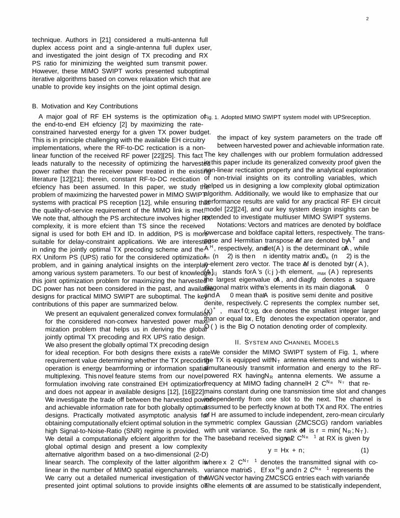
Fig. 1. Adopted MIMO SWIPT system model with UPS ρ reception.
the impact of key system parameters on the trade offbetween harvested power and achievable information rate.
The key challenges with our problem formulation addressedin this paper include its generalized convexity proof given thenon-linear rectification property and the analytical explorationof non-trivial insights on its controlling variables, whichhelped us in designing a low complexity global optimizationalgorithm. Additionally, we would like to emphasize that ourperformance results are valid for any practical RF EH circuitmodel [22]–[24], and our key system design insights can beextended to investigate multiuser MIMO SWIPT systems.
Notations: Vectors and matrices are denoted by boldfacelowercase and boldface capital letters, respectively. The trans-pose and Hermitian transpose of A are denoted by AT andAH, respectively, and det(A) is the determinant of A, whileIn (n ≥ 2) is the n× n identity matrix and 0n (n ≥ 2) is then-element zero vector. The trace of A is denoted by tr (A),[A]i,j stands for A’s (i, j)-th element, λmax (A) representsthe largest eigenvalue of A, and diag{·} denotes a squarediagonal matrix with a’s elements in its main diagonal. A � 0and A � 0 mean that A is positive semi definite and positivedefinite, respectively. C represents the complex number set,(x)
+ , max {0, x}, dxe denotes the smallest integer largerthan or equal to x, E{·} denotes the expectation operator, andO (·) is the Big O notation denoting order of complexity.
II. SYSTEM AND CHANNEL MODELS
We consider the MIMO SWIPT system of Fig. 1, wherethe TX is equipped with NT antenna elements and wishes tosimultaneously transmit information and energy to the RF-powered RX having NR antenna elements. We assume afrequency flat MIMO fading channel H ∈ CNR×NT that re-mains constant during one transmission time slot and changesindependently from one slot to the next. The channel isassumed to be perfectly known at both TX and RX. The entriesof H are assumed to include independent, zero-mean circularlysymmetric complex Gaussian (ZMCSCG) random variableswith unit variance. So, the rank of H is r = min(NR, NT ).The baseband received signal y ∈ CNR×1 at RX is given by
y = Hx + n, (1)
where x ∈ CNT×1 denotes the transmitted signal with co-variance matrix S , E{xxH} and n ∈ CNR×1 represents theAWGN vector having ZMCSCG entries each with variance σ2.The elements of x are assumed to be statistically independent,
3
Received RF power (dBm)-8 -4 0 4 8 12 16 20H
arvestedDC
pow
er(dBm)
-20
-10
0
10
20
30
RF-to-D
Ceffi
cien
cyη(·)(%
)
0
20
40
60
80
100Harvested DC power
RF-to-DC efficiency
(a) P1110 EVB characteristics [24].
Received RF power (dBm)-15 -13 -11 -9 -7 -5H
arvestedDC
pow
er(dBm)
-21
-18
-15
-12
-9
RF-to-D
Ceffi
cien
cyη(·)(%
)
30
35
40
45
50Harvested DC power
RF-to-DC efficiency
(b) RF EH circuit designed in [26].
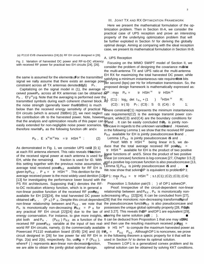
Fig. 2. Variation of harvested DC power and RF-to-DC efficiencywith received RF power for practical two EH circuits [24], [26].
the same is assumed for the elements of n. For the transmittedsignal we finally assume that there exists an average powerconstraint across all TX antennas denoted by tr (S) ≤ PT .
Capitalizing on the signal model in (1), the average re-ceived power PR across all RX antennas can be obtained asPR , E{yHy}. Note that the averaging is performed over thetransmitted symbols during each coherent channel block. Asthe noise strength (generally lower than −80dBm) is muchbelow than the received energy sensitivity of practical RFEH circuits (which is around −20dBm) [2], we next neglectthe contribution of n to the harvested power. Note, however,that the analysis and optimization results of this paper can beeasily extended for non-negligible noise power scenarios. Wetherefore rewrite PR as the following function of H and x
PR , E{xHHHHx
}= tr
(HSHH
). (2)
As demonstrated in Fig. 1, we consider UPS ratio ρ ∈ [0, 1]at each RX antenna element. This ratio reveals that ρ fractionof the received signal power at each antenna is used for RFEH, while the remaining 1 − ρ fraction is used for ID. Withthis setting together with the previous noise assumption, theaverage total received power PR,E available for RF EH isgiven by PR,E , ρPR = ρ tr
(HSHH
). This definition for the
average received power is the most widely used definition [12],[13] for investigating the performance lower bound with thePS RX architectures. Supposing that η (·) denotes the RF-to-DC rectification efficiency function, which is in general anon-linear positive function of the received RF power PR,Eavailable for EH [22]–[24], the total harvested DC power isobtained as PH , η (ρPR) ρPR. Despite this circuit dependentnon-linear relationship between η and PR,E , we note thatPH is monotonically non-decreasing in PR,E = ρPR forany practical RF EH circuit [22]–[24] due to the law ofenergy conservation. For instance, to give more insights, weplot both η and PH , η (PR,E) PR,E as a function of thereceived RF power PR,E variable at the input of two real-world RF EH circuits, namely, (i) the commercially availablePowercast P1110 evaluation board (EVB) [24] and (ii) thecircuit designed in [26] for low power far field RF EH inFigs. 2(a) and 2(b), respectively. So, using PH = F (PR,E),where F (·) represents a non-linear non-decreasing function,we are able to obtain the jointly global optimal design.
III. JOINT TX AND RX OPTIMIZATION FRAMEWORK
Here we present the mathematical formulation of the op-timization problem. Then in Section III-A, we consider thepractical case of UPS reception and prove an interestingproperty of the underlying optimization problem that willbe further exploited in Section IV for deriving the globallyoptimal design. Aiming at comparing with the ideal receptioncase, we present its mathematical formulation in Section III-B.
A. UPS Reception
Focusing on the MIMO SWIPT model of Section II, weconsider the problem of designing the covariance matrix S atthe multi-antenna TX and UPS ratio ρ at the multi-antennaEH RX for maximizing the total harvested DC power, whilesatisfying a minimum instantaneous rate requirement R in bitsper second (bps) per Hz for information transmission. So, theproposed design framework is mathematically expressed as:
OP : maxρ,S
PH = η(ρ tr
(HSHH
))ρ tr
(HSHH
)s.t. (C1) : log2
(det(INR + (1− ρ)σ−2HSHH
))≥ R,
(C2) : tr (S) ≤ PT , (C3) : S � 0, (C4) : 0 ≤ ρ ≤ 1,
where constraint (C1) represents the minimum instantaneousrate requirement, (C2) is the average transmit power con-straint, while (C3) and (C4) are the boundary conditions forS and ρ. It can be easily concluded that PH is jointly non-concave in regards to the unknown variables S and ρ. However,in the following Lemma 1 we show that the received RF powerPR,E available for EH is jointly pseudoconcave in S and ρ.
Lemma 1: PR,E is jointly pseudoconcave in S and ρ.Proof: With tr
(HSHH
)being linear in S, we de-
duce that the total average received RF power PR,E =ρ tr
(HSHH
)available for EH is the product of two positive
linear functions of ρ and S. Since the product of two positivelinear (or concave) functions is log-concave [27, Chapter 3.5.2]and a positive log-concave function is also pseudoconcave [13,Lemma 5], PR,E is jointly pseudoconcave in S and ρ.We now show that solving OP is equivalent to problem OP1:
OP1: maxρ,S
PR,E = ρ tr(HSHH
), s.t. (C1), (C2), (C3), (C4).
Proposition 1: Solution pair (S∗, ρ∗) of OP1 solves OP .Proof: Irrespective of the circuit-dependent non-linear
relationship between η and PR,E , PH is monotonically non-decreasing in PR,E [22]–[24]. It can be concluded from [27],[28] that the monotonic non-decreasing transformation PH ofthe pseudoconcave function PR,E is also pseudoconcave andpossesses the unique global optimality property [28, Props. 3.8and 3.27]. This reveals that OP and OP1 are equivalent [29],sharing the same solution pair (S∗, ρ∗).It can be deduced from Proposition 1 that one may solve OP1and then use the resulting maximum received power P ∗R,E =
ρ∗ tr(HS∗HH
)to compute the maximum harvested power as
P ∗H = η(P ∗R,E
)P ∗R,E . Although OP1 is nonconvex, we prove
in the following theorem a specific property for it that will beused in Section IV to derive its optimal solution.
Theorem 1: OP1 is a generalized convex problem and itsoptimal solution can be obtained by solving KKT conditions.
4
Proof: As shown in Lemma 1, PR,E is jointly pseudo-concave in S and ρ. It follows from constraint (C1) that thefunction R−log2
(det(INR + (1− ρ)σ−2HSHH
))is jointly
convex on ρ and S; this ensues from the fact that the matrixinside the determinant is a positive definite matrix [12], [17]–[19]. In addition, constraints (C2) and (C3) are linear withrespect to S and independent of ρ, and constraint (C4) dependsonly on ρ and is convex. The proof completes by combiningthe latter findings and using them in [29, Theorem 4.3.8].
Capitalizing on the findings of Proposition 1 and Theorem 1,we henceforth focus on the maximization of the receivedRF power PR,E for EH. The jointly optimal TX precodingand UPS design for this problem will also result in themaximization of the harvested DC power P ∗H for any practicalRF EH circuitry. Also, the proposed joint transceiver designin this paper is different from the ones in existing works [12]–[21] considering the received RF power for EH as a constraintand using a trivial linear RF EH model for their investigation.
B. Ideal Reception
To investigate the theoretical upper bound for PR,E , we nowconsider an ideal RX architecture capable of using all receivedRF power for both EH and ID. In particular, we remove ρ fromOP1 and (C1) and consider the following optimization:
OP2 :maxS
PR = tr(HSHH
), s.t. (C2), (C3),
(C5) : log2(det(INR + σ−2HSHH
))≥ R.
From the findings in the proof of Theorem 1, the objectivefunction PR of OP2 along with constraints (C2) and (C3) arelinear in S. In addition, (C5) is convex due to the concavity oflogarithm with respect to S. Combining the latter facts yieldsthat OP2 is a convex problem, and hence, its optimal solutioncan be found using the Lagrangian dual method [27], [29].
IV. OPTIMAL TX PRECODING AND RX POWER SPLITTING
Here, we first investigate trade off between energy beam-forming and information spatial multiplexing in OP1. Then,we present the global optimal solutions for OP1 and OP2.
A. Energy Beamforming versus Spatial Multiplexing
Let us consider the reduced Singular Value Decomposition(SVD) of the MIMO channel matrix H = UΛVH, whereV ∈ CNT×r and U ∈ CNR×r are unitary matrices andΛ ∈ Cr×r is the diagonal matrix consisting of the r non-zero eigenvalues of H in decreasing order of magnitude.Ignoring the rate constraint (C1) in OP1 (or equivalentlyin OP) leads to the rank-1 optimal TX covariance matrixS∗ = SEB , PT v1v
H1 [12], [30], where v1 ∈ CNT×1 is the
first column of V that corresponds to the eigenvalue [Λ]1,1 ,√λmax (HHH). This TX precoding, also known as transmit
energy beamforming, allocates PT to the strongest eigenmodeof HHH and is known to maximize the harvested or receivedpower. On the other hand, it is also well known [31] thatone may profit from the existence of multiple antennas andchannel estimation techniques to realize spatial multiplexingof multiple data streams. Spatial multiplexing adopts the
Rate constrainttransmit energybeamforming
Spatial multiplexing forrate constraint harvested
power maximization
Rth
p1 = PT , pi = 0,∀i = 2, 3, . . . , r
p1 < PT , pi ≥ 0,∀i = 2, 3, . . . , r
Rate constraint R
Rec
eive
dpo
wer
P∗ R,E
Rmax0
PT [Λ]21,1
Fig. 3. Trade off between received power for EH and achievableinformation rate. Rth is the switching point between TX precodingmodes: energy beamforming and information spatial multiplexing.
waterfilling technique to perform optimal allocation of PTover all the available eigenchannels of MIMO channel matrix.Evidently, for our problem formulation OP1 including the rateconstraint (C1) and PS reception, we need to investigate theunderlying fundamental trade off between TX energy beam-forming and information spatial multiplexing. As previouslydescribed, these two transmission schemes have contradictoryobjectives, and thus provide different TX designs.
Suppose we adopt energy beamforming in OP1, resultingin the received RF power PR
EB, ρ
EBPT [Λ]21,1 where ρ
EB
represents the unknown UPS parameter. To find the optimalUPS parameter ρ∗
EB, we need to seek for the best power
allocation (1−ρ∗EB
) for ID meeting the rate requirement R. Todo so, we solve (C1) at equality over UPS parameter yielding
ρ∗EB
, max{0, 1−
(2R − 1
)σ2[PT [Λ]21,1
]−1}. (3)
It can be concluded that both ρ∗EB
and the maximum receivedRF power given by ρ∗
EBPT [Λ]21,1 are decreasing functions
of R. This reveals that there exists a rate threshold Rth
such that, when R > Rth, one should allocate PT overto at least two eigenchannels instead of performing energybeamforming, i.e., instead of assigning PT solely to thestrongest eigenchannel. We are henceforth interested in find-ing this Rth value. Consider the optimum power allocationp∗1 and p∗2 for the two highest gained eigenchannels witheigenmodes [Λ]1,1 and [Λ]2,2, respectively, with [Λ]1,1 >[Λ]2,2. By substituting these values into (C1), defining Z1 ,√(
[Λ]21,1p∗1 − [Λ]22,2p
∗2
)2+ 2R+2[Λ]21,1[Λ]22,2p
∗1p∗2, and solv-
ing at equality for the optimum UPS parameter ρ∗SM2
for spatialmultiplexing over two eigenchannels deduces to
ρ∗SM2
, 1 +σ2
2
(1
[Λ]21,1p∗1
+1
[Λ]22,2p∗2
+Z1
[Λ]21,1[Λ]22,2p∗1p∗2
),
(4)
resulting in the maximum received RF power for EH givenby ρ∗
SM2
(p∗1 [Λ]21,1 + p∗2 [Λ]22,2
). We now combine the latterly
obtained maximum received RF power with spatial multiplex-ing and that of energy beamforming to compute Rth. Therate threshold value that renders energy beamforming more
5
beneficial than spatial multiplexing in terms of received RFpower can be obtained from solution of following inequality
ρ∗EBPT [Λ]21,1 > ρ∗
SM2
(p∗1 [Λ]21,1 + p∗2 [Λ]22,2
). (5)
Substituting (3) and (4) into (5), defining Z2 , ([Λ]21,1 −[Λ]22,2)([Λ]21,1p
∗1 + p∗2[Λ]22,2)
2, and applying some algebraicmanipulations yields the desired threshold in closed-form:
Rth , log2
(1 +
p∗2([Λ]21,1 − [Λ]22,2)
σ2+
√Z2
[Λ]21,1[Λ]22,2σ2p∗1
).
(6)Remark 1: The rate threshold Rth given by (6) evinces a
switching point on the desired TX precoding operation, whichis graphically presented in Fig. 3. When the rate requirementR is less or equal to Rth, energy beamforming is sufficient tomeet R, and hence, can be used for maximizing the receivedRF power. For cases where R > Rth, statistical multiplexingneeds to be adopted for maximizing the received RF powerfor EH while satisfying R. This explicit non-trivial switchingpoint Rth for the TX precoding mode is unique to theproblem formulation considered in this paper, and has not beenexplored or investigated in the relevant literature [12], [16]–[22] for the complementary problem formulations therein.We next use Rth in (6) to obtain solutions for OP1 and OP2.
B. Globally Optimal Solution of OP1Associating Lagrange multipliers µ and ν with constraints
(C1) and (C2), respectively, while keeping (C3) and (C4)implicit, the Lagrangian function of OP1 is defined as
the global optimal solution (S∗, ρ∗) for OP1 is obtained fromthe following four Karush-Kuhn-Tucker (KKT) conditions(the subgradient and complimentary slackness conditions aredefined, whereas the primal feasibility (C1)–(C4) and dualfeasibility constraints µ, ν ≥ 0 are kept implicit):
∂L∂S
=µ (1− ρ)σ2 ln 2
HHZ−13 H + ρHHH− νINT = 0, (8a)
∂L∂ρ
= −µ tr
(HSHH
σ2 ln 2Z−13
)+ tr
(HSHH
)= 0, (8b)
µ (R− log2 [detZ3]) = 0, (8c)
ν (tr (S)− PT ) = 0. (8d)
Solving (8) yields the KKT point [27], [29] defined by theoptimal solution (S∗, ρ∗, µ∗, ν∗). It is noted that it must holdν 6= 0, because the total available transmit power PT is alwaysfully utilized due to the monotonically increasing nature ofthe objective function PR,E in S. This implies that tr (S) =PT , which means that constraint (C2) is always satisfied atequality. Similarly, it must hold µ 6= 0, because the receivedRF power is strictly increasing in ρ and, as such, the fraction1− ρ allocated for ID needs to be sufficient in meeting (C1).
Recalling the trade off discussion in Section IV-A, whenR ≤ Rth, the optimal TX covariance matrix is given as S∗ =
SEB
. For this case the optimum TX precoding operation isenergy beamforming, i.e., F , V(P∗)1/2 ∈ CNT×r where ther × r matrix P∗ is defined as P∗ = diag{[PT 0 · · · 0]}, andthe optimal UPS ratio is ρ
EBgiven by (3). Substituting S
EB
and ρEB
into (8a) and (8b), yields corresponding multipliers:
µEB
, σ2 ln 2(1 +
(1− ρEB)PT [Λ]21,1σ2
), (9a)
νEB
,µ
EB(1− ρ
EB) [Λ]21,1
ln(2)(σ2 + (1− ρEB)PT [Λ]21,1
) + [Λ]21,1ρEB. (9b)
We therefore conclude that (S∗, ρ∗, µ∗, ν∗) is given as(SEB , ρEB , µEB , νEB) for R ≤ Rth. When R > Rth, theoptimum TX precoding operation is spatial multiplexing andwe thus to obtain the TX covariance matrix, rewrite (8a) inthe following form after applying algebraic simplifications.
ΛVHS VΛ =µ
ln 2
(ν Ir − ρΛHΛ
)−1Λ2 − σ2
1− ρ Ir. (10)
By performing the necessary left and right multiplications of(10) with Λ−1, V, and VH and setting ρ, µ, and ν to theiroptimal values ρ
SM, µ
SM, and ν
SMfor spatial multiplexing, the
optimal TX covariance matrix for R > Rth can be derived as:
SSM
= V
µSM
(νSM
Ir − ρSMΛHΛ
)−1ln 2
− σ2Λ−2
1− ρSM
VH.
(11)On simplifying (8b) to solve for the optimal µSM yields
µSM
=tr(HS
SMHH)
tr(
HSSM
HH
σ2 ln 2 (INR + (1− ρSM
)σ−2HSSM
HH)−1) .
(12)Evidently from (11), SSM ∈ CNT×NT can be expressedas S
SM, VP∗VH with the r × r matrix P∗ ,
diag{[p∗1 p∗2 · · · p∗r ]} representing the optimal power allocationmatrix among H’s eigenchannels, whose entries are given by
p∗k =
µ∗
ln 2(νSM− ρ
SM[Λ]2k,k
) − σ2
(1− ρSM
) [Λ]2k,k
+
. (13)
The optimal ρSM
, µSM
, and νSM
is the solution of the systemwith the three equations (8c), (8d), and (12) after settingS = S
SMand satisfying µ, ν > 0 and 0 ≤ ρ < 1. Later
in Section VI we first reduce this system of equations to two,and then by exploiting the tight bounds on ν∗ derived in Sec-tion V-A2, we present how it can be efficiently implemented.
Remark 2: Observing (11) and (13) leads to the conclusionthat the optimum TX precoding for R > Rth is F =V(P∗)1/2 with the r diagonal elements of P∗ given by (13).This precoding results in r parallel eigenchannel transmissionswith power allocation obtained from a modified waterfillingalgorithm, where water levels depend on R, PT , H, and σ2.
By combining these results for energy beamforming andspatial multiplexing, the optimal solution of OP1 is given by
S∗ =
PT v1v
H1 , R ≤ Rth ≤ Rmax,
V(µ∗ Z4
ln 2 − σ2Λ−2
1−ρ
)VH, Rth < R ≤ Rmax,
Infeasible, R > Rmax,
(14)
6
where Z4 ,(ν∗Ir − ρΛHΛ
)−1, ρ∗ = ρEB , µ∗ = µEB , and
ν∗ = νEB for R ≤ Rth, and for R > Rth, ρ∗ = ρSM , µ∗ =µSM , and ν∗ = νSM are obtained from the solution of thesystem of equations described below (13). The feasibility ofOP1 depends on Rmax , log2
(det(INR + σ−2HS
WFHH))
,which represents the maximum achievable rate for UPS ratioρ = 0 and S
WF, VP
WFVH. In the latter expression, P
WF,
diag{[pWF,1 pWF,2 · · · pWF,r ]} is the r × r power allocationmatrix whose rank rw (non-zero diagonal entries) is [32]
rw , max
{k
∣∣∣∣∣ PT −k−1∑i=1
(σ2
[Λ]2k,k− σ2
[Λ]2i,i
)> 0, k ≤ r
}(15)
and its non-zero elements with index k = 1, 2, . . . , rw areobtained from the standard waterfilling algorithm as
pWF,k
=
PT −rw−1∑i=1
(σ2
[Λ]2rw,rw− σ2
[Λ]2i,i
)rw
+σ2
[Λ]2rw,rw− σ2
[Λ]2k,k.
(16)Here we would like to add that based on (14) deciding
whether the optimal TX precoding matrix S∗ is denoted SEB
orS
SM, the corresponding optimal TX signal vector x∗ ∈ CNT×1
can be obtained as xEB
,√PT v1 x and x
SM, V (P∗)
1/2x.
Here x is an arbitrary ZMCSCG signal and x ∈ Cr×1 is aZMCSCG random vector, both having unit variance entries.
C. Globally Optimal Solution of OP2Like OP1, the proposed rate threshold value in OP2
determining the optimal TX precoding operation, is given by
Ridth , log2
(1 + σ−2PT [Λ]21,1
), (17)
represents rate achieved by energy beamforming for ideal RX.Lemma 2: Global optimal solution S∗id of OP2 is given by
S∗id=
PT v1v
H1 , R ≤ Rid
th ≤ Rmax,Vdiag{[p(id)1 p
(id)2 · · · p(id)r ]}VH, Rid
th < R ≤ Rmax,Infeasible, R > Rmax,
(18)with p(id)k denoting power assignment to k-th eigenchannel is
p(id)k =
µ∗2
ln 2(ν∗2 − [Λ]2k,k
) − σ2
[Λ]2k,k
+
, ∀k = 1, 2, . . . , r.
(19)In the latter expression, ν∗2 ≥ 0 and µ∗2 ≥ 0 represent
the Lagrange multipliers corresponding to constraints (C2)and (C5), respectively. These can be obtained using a sub-gradient method as described in [12, App. A] such thatlog2
(det(INR + σ−2HS∗idH
H))
= R and tr (S∗id) = PT .Proof: The proof is provided in Appendix A.
Remark 3: It can be observed from the solution of OP2that our proposed TX precoding design significantly differsfrom that obtained from the solution of optimization problem(P3) in [12]. This reveals that the design maximizing thetotal received RF power for EH, while satisfying a minimuminstantaneous rate requirement, is very different from thedesign that maximizes the instantaneous rate subject to aminimum constraint on the total received RF power.
V. ANALYTICAL BOUNDS AND ASYMPTOTIC RELAXATION
Here we first present analytical bounds for the UPS ratio ρand Lagrange multipliers µ, ν defined in Section IV. Then tightasymptotic approximations for the joint design are presented.
A. Analytical Bounds
1) UPS Ratio ρ: The information rate is given bylog2
(det(INR + (1− ρ)σ−2HSHH
)), which is a monoton-
ically decreasing function of ρ. The upper bound ρUB
on thefeasible ρ value satisfying (C1) is given by the UPS ratiocorresponding to the maximum achievable rate value Rmax
as achieved with statistical multiplexing over all availableeigenchannels. Mathematically, ρUB as obtained by settingS = VPWFVH with the entries of PWF defined in (16), is
ρUB ,
{ρ
∣∣∣∣det(INR +(1− ρ)HSWFHH
σ2
)= 2R, ρ ≤ 1
}.
(20)Likewise, the lower bound on the feasible ρ meeting (C1) isgiven by the UPS ratio ρEB defined in (3). This lower boundhappens with energy beamforming, where entire TX power isallocated to the best gain eigenchannel and the achievable rateis minimum. Combining these results, yields ρ
EB≤ ρ ≤ ρ
UB.
2) Lagrange Multipliers µ and ν for R > Rth: Tohave non-negative power allocation p1 over the best gaineigenchannel having eigenmode [Λ]1,1, it must hold from(13) that ν ≥ ν
LB, ρ [Λ]21,1. Also, using the definition
p1 = αPT with α ≤ 1 in (13) for k = 1 yields µ =(ν − ρ[Λ]21,1
) (αPT + σ2
(1−ρ)[Λ]21,1
)ln 2. Since for the total
received power holds tr(HSHH
)≤ PT and also (12) holds,
the upper bound for µ, denoted by µUB , can be obtained as
µ(a)<
(1− ρ) ln 2 tr(HSHH
)r
< µUB
,(1− ρ)PT ln 2
r(21)
where (a) results from the high SNR approximation. Combin-ing (21) with σ2
(1−ρ)[Λ]21,1> 0, leads to ν < (1−ρ)
α r + ρ[Λ]21,1.Due to the highest power allocation over the best gain eigen-channel, it must hold α ≥ 1
r , yielding νUB , 1+ρ([Λ]21,1−1).However as shown later, ν � ν
UBbecause the total received
power PR � PT . These bounds will be used in Section VI-Bfor efficiently implementing the global optimization algorithm.
B. Asymptotic Analysis
The received RF power for EH in SWIPT systems needs tobe greater than energy reception sensitivity [2], [3], whichis in the order of −10dBm to −30dBm, for having non-zero harvested DC power after rectification. Since, the AWGNpower spectral density is around −175dBm/Hz leading to anaverage received noise power of around −100dBm for SWIPTat 915 MHz, the received SNR in practical SWIPT systemsis very high, i.e., around 70dB, even for very high frequencytransmissions. Based on this practical observation for SWIPT,we next investigate the joint design for high SNR scenarios.
7
1) Globally Optimal Solution of OP1 for High SNR: Theoptimal solution of OP1 for high SNR values defined as(S∗a, ρ
∗a, µ∗a, ν∗a) can be obtained similarly to Section IV-B as
S∗a=
PT v1v
H1 , R ≤ Rth ≤ Rmax,
V
(µ∗a(ν
∗aIr−ρ∗a ΛHΛ)
−1
ln 2
)VH, Rth < R ≤ Rmax ,
Infeasible, R > Rmax,
(22)
µ∗a = r−1 (1− ρ∗a) tr(HS∗aHH
)ln 2, and the remaining two
unknowns ρ∗a and ν∗a are given from the solutions of the equa-tions tr (S∗a) = PT and log2
(det(σ−2 (1− ρ)HS∗aHH
))=
R. After some simplifications with (22), the power allocationis obtained as p∗a,k =
µ∗a
(ν∗a−ρ∗a[Λ]2k,k) ln 2
,∀k = 1, 2, . . . , r.
Hence, under high SNR, the optimal power allocation overavailable eigenchannels for R > Rth is always greater thanzero regardless of the relative strengths of the eigenmodes.
2) Globally Optimal Solution of OP2 for High SNR: Usingthe derived analytical bounds for ρ and ν along with Lemma 2,the asymptotic approximation S∗id,a for S∗id can be obtained as
(23)where each p(id,a)k with k = 1, 2, . . . , r is given by
p(id,a)k =
µ∗2a(ν∗2a − [Λ]2k,k
)ln 2
. (24)
With [Λ]21,1 < ν∗2a < [Λ]21,1 + 1, solving∑rk=1 p
(id,a)k = PT
yields µ∗2a = PT
(r∑
k=1
1
(ν∗2a−[Λ]2k,k) ln 2
)−1. Setting β , ν∗2a−
[Λ]21,1 and substituting in (24), we can rewrite p(id,a)k as
p(id,a)k = β p
(id,a)1
[β + [Λ]21,1 − [Λ]2k,k
]−1. (25)
To solve for β ∈ (0, 1), we need to replace into the rate
constraint expression leading tor∏
k=1
(p(id,a)k [Λ]2k,k
σ2
)= 2R,
which after some simplifications results in the expressionr∏
k=1
(β [Λ]2k,k
β + [Λ]21,1 − [Λ]2k,k
)= 2R
(σ2
p(id,a)1
)r. (26)
The p(id,a)1 in (26) can be obtained in closed-form as a functionof β by solving
∑rk=1 p
(id,a)k = PT and using (25), yielding
p(id,a)1 = PT
(1 +
r∑k=2
(β
β + [Λ]21,1 − [Λ]2k,k
))−1. (27)
Using these developments in Section VI-B3 we show that theasymptotically optimal TX precoding forOP2 can be obtainedusing a 1-D linear search over very short range (0, 1) of β.
Remark 4: With the expressions (26) and (27) resulted fromour derived asymptotic analysis, we have managed to replacethe problem of finding the positive real values of µ2 and ν2in OP2 along with the required waterfilling-based decisionmaking process
(involving a discontinuous function (x)
+ dueto underlying (C3)
)by a simple linear search over β ∈ (0, 1).
VI. EFFICIENT GLOBAL OPTIMIZATION ALGORITHM
The goal here is to first present a global optimizationalgorithm to obtain the previously derived optimal solutionsfor OP1 and OP2 by effectively solving the KKT conditions.After that we present an alternate low complexity algorithmbased on a simple 2-D linear search to practically implementthe former algorithm in a computational efficient manner.
A. Solving the KKT Conditions
As discussed in Section IV, S∗ and ρ∗ of OP1 forR > Rth are obtained by solving (8c), (8d), and (12)for ρ∗, µ∗, and ν∗ after setting S = S
SM. Likewise, from
Lemma 2, S∗id of OP2 for R > Ridth is derived by solving
log2
(det(INR+
HS∗idH
H
σ2
))=R and tr (S∗id)=PT in µ∗2 and ν∗2 .
1) Reduction of the System of Non-linear Equations: It isin general very difficult to efficiently solve a large system ofnon-linear equations. Hereinafter, we discuss the reduction ofthe number of the non-linear equations to be solved from threeto two in OP1 and from two to one in OP2.
Let us denote the rank of the optimal TX covariance matrixby rs. It represents the number of eigenchannels that havenon-zero power allocation, i.e., pk > 0 with k = 1, 2, . . . , rs.Substituting this definition into (8d) and (13) with ν > 0, wecan express µ∗ in terms of ν∗ and ρ∗ as
µ∗ =PT +
∑rsk=1 σ
2((1− ρ∗) [Λ]2k,k
)−1rs∑rsk=1
((ν∗ − ρ∗[Λ]2k,k
)ln 2)−1 . (28)
Using definition of rs in (8c) and (13) with µ > 0, we obtain
µ∗=2Rrs σ2
((1− ρ∗)
(rs∏k=1
[Λ]2k,kν∗ − ρ∗[Λ]2k,k
) 1rs )−1
ln 2. (29)
By combining (12), (28), and (29), the reduced system of twonon-linear equations to be solved for ρ∗ and ν∗ as included inKKT point (S∗, ρ∗, µ∗, ν∗) for R > Rth in OP1 is given by
PT (1− ρ∗)σ−2 +∑rsk=1[Λ]−2k,k
2Rrs rs
∑rsk=1
(ν∗ − ρ∗[Λ]2k,k
)−1 =
(rs∏k=1
[Λ]2k,kν∗ − ρ∗[Λ]2k,k
)− 1rs
(30a)
rs∑k=1
p∗k [Λ]2k,k (1− ρ∗)−1
1 + (1− ρ∗) p∗k [Λ]2k,k=
rs∑k=1
p∗k [Λ]2k,k
(rs∏j=1
[Λ]2j,jν∗−ρ∗[Λ]2j,j
) 1rs
2Rrs σ2 ln 2
(30b)
where p∗k = σ2
(1−ρ∗)
(2Rrs (ν∗−ρ∗[Λ]2k,k)
−1(∏rsj=1
[Λ]2j,j
ν∗−ρ∗[Λ]2j,j
) 1rs
− 1[Λ]2k,k
)+
,∀k =
1, 2, . . . , rs. In a similar manner, the single non-linear equationthat needs to be solved for computing ν∗2 included in the KKTpoint (S∗id, µ
∗2, ν∗2 ) for R > Rid
th in OP2 is given by(PTσ2
+
rs∑j=1
1
[Λ]2j,j
)( rs∏k=1
[Λ]2k,kν∗2 − [Λ]2k,k
) 1rs
=
rs∑k=1
2Rrs rs
ν∗2 − [Λ]2k,k.
(31)
8
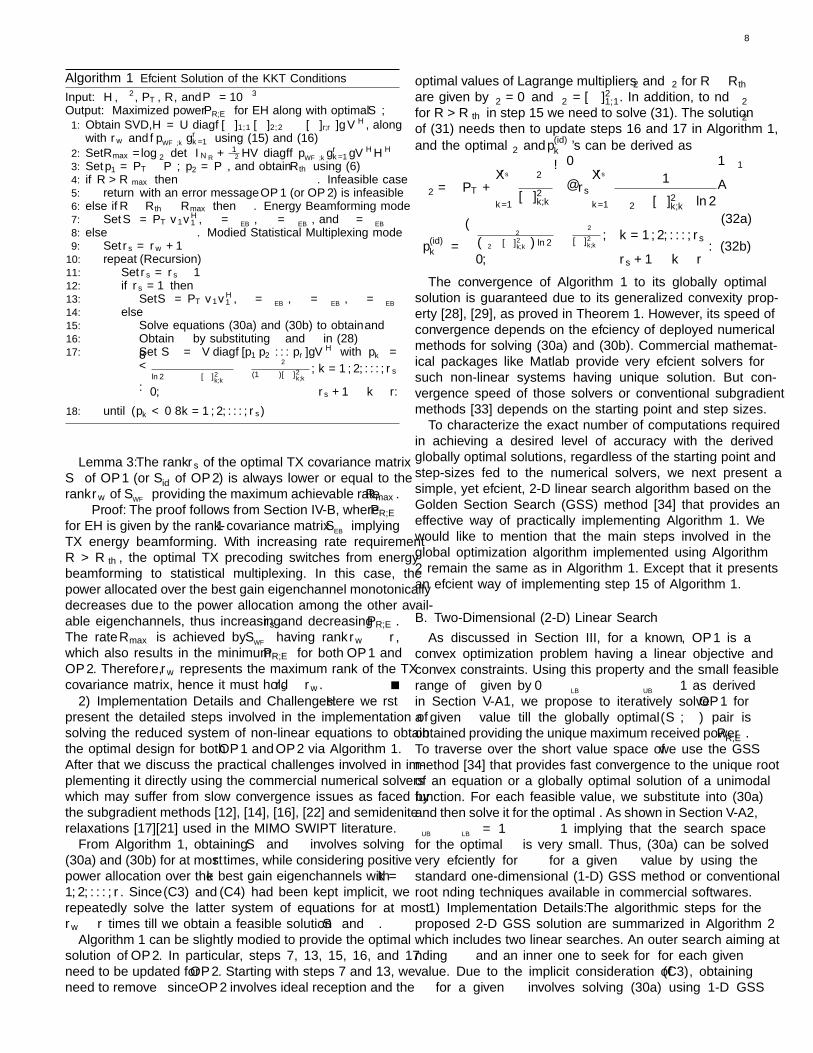
Algorithm 1 Efficient Solution of the KKT Conditions
Input: H, σ2, PT , R, and Pδ = 10−3
Output: Maximized power P ∗R,E for EH along with optimal S∗, ρ∗
1: Obtain SVD, H = U diag{[Λ]1,1 [Λ]2,2 · · · [Λ]r,r]}VH, alongwith rw and {pWF,k}
rk=1 using (15) and (16)
2: SetRmax =log2
(det(INR+ 1
σ2 HVdiag{{pWF,k}rk=1}VHHH
))3: Set p∗1 = PT − Pδ, p∗2 = Pδ , and obtain Rth using (6)4: if R > Rmax then . Infeasible case5: return with an error message – OP1 (or OP2) is infeasible6: else if R ≤ Rth ≤ Rmax then . Energy Beamforming mode7: Set S∗ = PT v1v
Lemma 3: The rank rs of the optimal TX covariance matrixS∗ of OP1 (or S∗id of OP2) is always lower or equal to therank rw of S
WFproviding the maximum achievable rate Rmax.
Proof: The proof follows from Section IV-B, where PR,Efor EH is given by the rank-1 covariance matrix SEB implyingTX energy beamforming. With increasing rate requirementR > Rth, the optimal TX precoding switches from energybeamforming to statistical multiplexing. In this case, thepower allocated over the best gain eigenchannel monotonicallydecreases due to the power allocation among the other avail-able eigenchannels, thus increasing rs and decreasing PR,E .The rate Rmax is achieved by S
WFhaving rank rw ≤ r,
which also results in the minimum PR,E for both OP1 andOP2. Therefore, rw represents the maximum rank of the TXcovariance matrix, hence it must hold rs ≤ rw.
2) Implementation Details and Challenges: Here we firstpresent the detailed steps involved in the implementation ofsolving the reduced system of non-linear equations to obtainthe optimal design for both OP1 and OP2 via Algorithm 1.After that we discuss the practical challenges involved in im-plementing it directly using the commercial numerical solverswhich may suffer from slow convergence issues as faced bythe subgradient methods [12], [14], [16], [22] and semidefiniterelaxations [17]–[21] used in the MIMO SWIPT literature.
From Algorithm 1, obtaining S∗ and ρ∗ involves solving(30a) and (30b) for at most r times, while considering positivepower allocation over the k best gain eigenchannels with k =1, 2, . . . , r. Since (C3) and (C4) had been kept implicit, werepeatedly solve the latter system of equations for at mostrw ≤ r times till we obtain a feasible solution S∗ and ρ∗.
Algorithm 1 can be slightly modified to provide the optimalsolution of OP2. In particular, steps 7, 13, 15, 16, and 17need to be updated for OP2. Starting with steps 7 and 13, weneed to remove ρ∗ since OP2 involves ideal reception and the
optimal values of Lagrange multipliers µ2 and ν2 for R ≤ Rth
are given by µ∗2 = 0 and ν∗2 = [Λ]21,1. In addition, to find ν∗2for R > Rth in step 15 we need to solve (31). The solution ν∗2of (31) needs then to update steps 16 and 17 in Algorithm 1,and the optimal µ∗2 and p(id)k ’s can be derived as
µ∗2 =
(PT +
rs∑k=1
σ2
[Λ]2k,k
)rs rs∑k=1
1(ν∗2 − [Λ]2k,k
)ln 2
−1(32a)
p(id)k =
{ µ∗2
(ν∗2−[Λ]2k,k) ln 2
− σ2
[Λ]2k,k, k = 1, 2, . . . , rs
0, rs + 1 ≤ k ≤ r. (32b)
The convergence of Algorithm 1 to its globally optimalsolution is guaranteed due to its generalized convexity prop-erty [28], [29], as proved in Theorem 1. However, its speed ofconvergence depends on the efficiency of deployed numericalmethods for solving (30a) and (30b). Commercial mathemat-ical packages like Matlab provide very efficient solvers forsuch non-linear systems having unique solution. But con-vergence speed of those solvers or conventional subgradientmethods [33] depends on the starting point and step sizes.
To characterize the exact number of computations requiredin achieving a desired level of accuracy with the derivedglobally optimal solutions, regardless of the starting point andstep-sizes fed to the numerical solvers, we next present asimple, yet efficient, 2-D linear search algorithm based on theGolden Section Search (GSS) method [34] that provides aneffective way of practically implementing Algorithm 1. Wewould like to mention that the main steps involved in theglobal optimization algorithm implemented using Algorithm2 remain the same as in Algorithm 1. Except that it presentsan efficient way of implementing step 15 of Algorithm 1.
B. Two-Dimensional (2-D) Linear Search
As discussed in Section III, for a known ρ, OP1 is aconvex optimization problem having a linear objective andconvex constraints. Using this property and the small feasiblerange of ρ given by 0 ≤ ρLB ≤ ρ ≤ ρUB ≤ 1 as derivedin Section V-A1, we propose to iteratively solve OP1 fora given ρ value till the globally optimal (S∗, ρ∗) pair isobtained providing the unique maximum received power P ∗R,E .To traverse over the short value space of ρ we use the GSSmethod [34] that provides fast convergence to the unique rootof an equation or a globally optimal solution of a unimodalfunction. For each feasible ρ value, we substitute into (30a)and then solve it for the optimal ν∗. As shown in Section V-A2,νUB− ν
LB= 1 − ρ ≤ 1 implying that the search space
for the optimal ν∗ is very small. Thus, (30a) can be solvedvery efficiently for ν∗ for a given ρ∗ value by using thestandard one-dimensional (1-D) GSS method or conventionalroot finding techniques available in commercial softwares.
1) Implementation Details: The algorithmic steps for theproposed 2-D GSS solution are summarized in Algorithm 2which includes two linear searches. An outer search aiming atfinding ρ∗ and an inner one to seek for ν∗ for each given ρvalue. Due to the implicit consideration of (C3), obtainingν∗ for a given ρ∗ involves solving (30a) using 1-D GSS
9
Algorithm 2 Global Optimization Algorithm based on 2-D GSS
Input: H, σ2, PT , R, and acceptable tolerance ξ � 1Output: Maximized P ∗
R,E for EH along with optimal S∗ and ρ∗
1: Follow steps 1, 2, and 3 of Algorithm 1 for initialization2: if R > Rmax then step 5 of Algorithm 1 . Infeasible case3: else if R ≤ Rth ≤ Rmax then step 7 of Algorithm 14: else . Modified Statistical Multiplexing mode5: Obtain ρLB and ρUB by respectively using (3) and (20). Then,
set ρp = ρUB − 0.618 (ρUB − ρLB)6: rs = rw + 1, νLB = ρp[Λ]21,1, and νUB = ρp[Λ]21,1 + 1− ρp7: repeat (Inner loop: Recursion over feasible ν range)8: Set rs = rs − 1, and check if rs = 1 to implement
step 13 of Algorithm 19: Substitute ρ∗ = ρp in (30a), and solve it to obtain ν∗ ∈
(νLB , νUB) using 1-D GSS10: Obtain µ∗ and p∗k by using steps 16 and 17 of Algorithm 111: until (p∗k < 0 ∀k = 1, 2, . . . , rs)12: Set P ∗
14: Repeat steps 6 to 12 with ρp being replaced by ρq in thesesteps to obtain P ∗
R,E , p∗k, µ
∗, and ν∗ for ρ∗ = ρq15: Set PR,q = P ∗
R,E , µq = µ∗, νq = ν,c = 0,∆ρ = ρUB − ρLB
16: while ∆ρ > ξ do (Outer loop: Recursion over feasible ρ)17: if PR,p ≥ PR,q then18: Set ρUB = ρq , ρq = ρp, PR,q = PR,p, and ρp =
ρUB − 0.618 (ρUB − ρLB)19: Repeat steps 6 to 12 with ρ∗ = ρp and set the results
as PR,p = P ∗R,E , µp = µ∗, νp = ν∗
20: else21: Set ρLB = ρp, ρp = ρq , PR,p = PR,q , and ρq =
ρLB + 0.618 (ρUB − ρLB)22: Repeat steps 6 to 12 with ρp replaced by ρq and to
obtain PR,q = P ∗R,E , µq = µ∗, νq = ν∗
23: Set c = c+ 1 and ∆ρ = ρUB − ρLB
for at most rw ≤ r times, while considering positive powerallocation over the k = 1, 2, . . . , r best gain eigenchannels.
Algorithm 2 can also be slightly modified to be used forobtaining the solution for OP2, where due to ideal reception,the outer GSS over the feasible ρ values has to be removed andwe only need to perform a 1-D GSS for ν∗2 over its feasiblevalue range [Λ]21,1 ≤ ν∗2 ≤ [Λ]21,1+1. So, for OP2 we need toconsider steps 1–12 of Algorithm 2, excluding the initializationstep 5, and updating steps 6, 9, 10, and 12. Particularly, thebounds are given by ν2LB = [Λ]21,1 and ν2UB = [Λ]21,1 + 1 instep 6. In step 9, we need to solve (31) to find optimal ν∗2for R > Rth. This ν∗2 value will then be used in step 10 toobtain the optimal µ∗2 and p
(id)k ’s by substituting ν∗2 in (32a)
and (32b). Lastly, we need to set ρ∗ = 1 in step 12.2) Complexity Analysis: Suppose that we want to calculate
ρ∗ and ν∗ of OP1 or ν∗2 of OP2 through Algorithm 2 soas to be close up to an acceptable tolerance ξ � 1 to theirglobally optimal solutions. As seen from Algorithm 2, thesearch space interval after each GSS iteration reduces by afactor of 0.618 [34, Chap. 2.5]. This value combined withthe unity maximum search length for ρ∗ and ν∗ gives thenumber of iterations c∗ =
⌈ln(ξ)
ln(0.618)
⌉+ 1 that are required to
ensure that the numerical error is less than ξ. For example,ξ = 10−3 results in c∗ = 16. Note that c∗ is a logarithmicfunction of ξ and is independent of NT , NR, and r. Aseach computation in GSS iteration for finding ρ∗ involves an
inner GSS for computing ν∗, which is repeated for at mostrw runs, the total number of iterations required for findingthe globally optimal solution of OP1 within an acceptabletolerance ξ is given by c∗1 ≤ rw c∗ (c∗ + 1). Since the numberof function computations in GSS is one more than the numberof iterations and rs ≤ rw ≤ r from Lemma 3, the totalnumber of computations involved in solving OP1 are bounded
by the value r(⌈
ln(ξ)ln(0.618)
⌉+ 2)2
. Hence, the computationalcomplexity of Algorithm 2 is O (r), i.e., linear in r. Thiscomplexity witnesses the significance of Algorithm 2 overAlgorithm 1. Instead of directly implementing commercial nu-merical solvers or subgradient methods [33] for Algorithm 1,we use the 2-D GSS method as outlined in Algorithm 2.
Regarding the required number of iterations c∗2 for findingthe solution of OP2 it must hold c∗2 ≤ rw c
∗ ≤ r c∗.As a result, the computational complexity of the modifiedAlgorithm 2 for OP2 is O
(r(⌈
ln(ξ)ln(0.618)
⌉+ 1))
= O (r).3) High SNR Approximation: Recalling Remark 4 in Sec-
tion V-B2 holding for high SNR values and focusing onequations (26) and (27) for R > Rth, it becomes apparent that,since p(id,a)k > 0 ∀k = 1, 2, . . . , r, then even with the implicitconsideration of (C3) one does not need to repeatedly solvethe 1-D GSS over ν∗2 . Thus, we only need to find β ∈ (0, 1)from the following equation using the 1-D GSS method:
PT
2Rr σ2
(r∏
k=1
β [Λ]2k,kβ+[Λ]21,1−[Λ]2k,k
) 1r
=r∑
k=1
(β
β+[Λ]21,1−[Λ]2k,k
). (33)
The computational complexity of finding the globally op-timal solution of OP2 for high SNR values is thereforeO(⌈
ln(ξ)ln(0.618)
⌉+ 1)= O (1), i.e., independent of r.
VII. NUMERICAL RESULTS AND DISCUSSION
In this section, we numerically evaluate the performance ofthe proposed joint TX precoding and RX UPS splitting design,and investigate the impact of various system parameters onits achievable rate-energy trade off. Unless otherwise stated,we set σ2 = {−100,−70}dBm by considering noise spectraldensity of −175 dBm/Hz as well as PT = 10W, and ξ = 10−4.Furthermore, we model H as H =
{θhij
∣∣1 ≤ i, j ≤ N} withN , NR = NT = {2, 4}, where θ = {0.1, 0.05} models thedistance dependent propagation losses and hij’s are ZMCSCGrandom variables with unit variance. With this definition, theaverage channel power gain is given by θ2 = a d−n, where ais the propagation loss constant, n is the path loss exponent,and d is the TX-to-RX distance. So, for a = 0.1 and n = 2,θ = 0.1 represents that d = 3.16 m. Whereas this separationbecomes twice, i.e., d = 6.32 m, for θ = 0.05. We assumeunit transmission block duration, thus, we use the terms‘received energy’ and ‘received power’ interchangeably. Allperformance results have been generated after averaging over103 independent channel realizations. For obtaining S∗ and ρ∗
with the proposed design we have simulated Algorithm 2.We consider 2× 2 and 4× 4 MIMO systems in Fig. 4 with
both ideal and UPS reception and illustrate the rate-energytrade off for our proposed designs for different valuesfor the propagation losses and noise variance parameters.
10
Rate constraint R (bps/Hz)60 80 100 120 140 1600
0.2
0.4
0.6
0.8
1
(b) 4× 4 MIMO system.
UPS Ideal
UPS Ideal
Rate constraint R (bps/Hz)30 40 50 60 70 80R
eceivedRFPow
erP
∗ R,E
forEH
(W)
0
0.1
0.2
0.3
0.4
0.5
(a) 2× 2 MIMO system.
θ = 0.1, σ2 = −100 dBm
θ = 0.1, σ2 = −70 dBm
θ = 0.05,σ2 = −100 dBmθ = 0.05,σ2 = −70 dBm
Fig. 4. Variation of the rate-energy trade off for varying parameters.
2, −70 2, −100 4, −70 4, −100
Harvestedpow
er(W
)
0.02
0.03
0.04
(b) Variation of harvested power PH
Number of antennas, AWGN power (N, σ2 in dBm)2, −70 2, −100 4, −70 4, −100
RF-D
Ceffi
cien
cyη(%
)
50
55
60
(a) Variation of rectification efficeincy
Rmax − 9 Rmax − 6 Rmax − 3
106.60
53.42
146.47
73.35
Fig. 5. Variation of η and PH for Powercast RF EH circuit [24] withrate R near Rmax for PT = 10W θ = 0.05, and different values forN and σ2. Also, Rmax is mentioned over the bars in (b).
As expected, our solution for OP2 with ideal receptionoutperforms that of OP1 that considers practical UPSreception. It is also obvious that increasing N improves therate-energy trade off. This happens because both beamformingand multiplexing gains improve as N gets larger. Lessernoisy systems, when σ2 decreases, and better channelconditions with increasing θ result in better trade off andenable higher achievable rates. The maximum achievable rateRmax in bps/Hz for the considered four cases
−100dBm)} is given by {53.42, 57.77, 73.35, 77.7} for
N = 2 and {106.60, 114.42, 146.47, 154.28} for N = 4.In addition, the average value of Rth in bps/Hz for thesecases is given by {17.27, 18.72, 26.02, 27.98} for N = 2 and{17.46, 19.05, 26.92, 28.73} for N = 4. When R < Rth,the maximum received RF power P ∗R,E for EH is achievedwith TX energy beamforming. However, as R increasesand becomes substantially larger than Rth, P ∗R,E decreasestill reaching a minimum value. For the latter cases, TXspatial multiplexing is adopted to achieve R and anyremaining received power is used for EH. Further, with θdecreasing as {0.1, 0.01, 0.001}, the corresponding Rmax
varies as {77.70, 64.06, 50.76} bps/Hz for N = 2 and{154.28, 127.89, 101.33} bps/Hz for N = 4. Whereas, thecorresponding P ∗R,E for EH with R = 0 bps/Hz varies as{0.36W, 3.52mW, 35.74µW} for N = 2 and {0.93W,10.09mW, 97.22µW} for N = 4 MIMO SWIPT systems.
Now considering Powercast RF EH circuit [24], we inves-tigate the impact of η on PH with varying rate requirementsclose to Rmax because in this regime the corresponding P ∗R,Edecreases sharply as shown in Fig. 4. For each of the four cases
Rate constraint R (bps/Hz)20 30 40 50 60 70 80P
ower
allocatedto
best
gain
eigenchan
nel,p∗ 1(W
)
5
6
7
8
9
10
θ = 0.1, σ2 = −100 dBm
θ = 0.1, σ2 = −70 dBm
θ = 0.05, σ2 = −100 dBm
θ = 0.05, σ2 = −70 dBm
Fig. 6. Variation of the optimal power allocation p∗1 of the best gaineigenchannel of a 2× 2 MIMO system as a function of rate R.
0.7 0.85 0.95 1
Optimal
pow
erallocationp∗ k’s
0
5
10(i) θ = 0.1,σ2 = −70 dBm
Normalized rate constraint RRmax
0.7 0.85 0.95 10
5
10(ii) θ = 0.05,σ2 = −70 dBm
p∗1p∗2p∗3p∗4
0.79.4
9.6
9.8
10
Fig. 7. Variation of optimal power allocation in a 4× 4 system as afunction of normalized rate R
Rmaxfor PT = 10W, σ2 = −70dBm.
of varying N and σ2 as plotted in Fig. 5, though η does notfollow any trend (increasing for first two cases and decreas-ing then increasing for the next two), PH is monotonicallydecreasing with increasing R from R = Rmax − 9 bps/Hz toR = Rmax− 3 bps/Hz, because this increase in rate R resultsin a lower P ∗R,E . So, this monotonic trend of optimized PHin P ∗R,E as depicted via Fig. 5 numerically corroborates thediscussion with respect to the claim made in Proposition 1.
The variation of optimal power allocation with the proposedjoint design for OP1 is depicted in Figs. 6 and 7 for 2 × 2and 4 × 4 MIMO systems, respectively, as a function of R.Particularly, Fig. 6 illustrates the optimal power allocation p∗1over the best gain eigenchannel for 2 × 2 system, while theoptimal power allocation p∗1, p∗2, p∗3, and p∗4 over the r = 4available eigenchannels is demonstrated in Fig. 7. As shown,p∗1 monotonically decreases from p∗1 uPT (this happens forR ≤ Rth where TX energy beamforming is adopted) to theequal power allocation p∗1 u p∗2 u PT
2 (for large R = Rmax,TX spatial multiplexing is used). As from (13), p∗1 ≥ p∗2, wenote that with PT = 10W for N = 2, p∗1 ≥ 5 W in Fig. 6. Asimilar trend is observed in Fig. 7. For the plotted normalizedrate constraint range, most of PT is allocated to the best gaineigenchannel to perform TX energy beamforming, while theremaining power is allocated to the rest eigenchannels formeeting rate requirement R with spatial multiplexing.
In Fig. 8, the optimal UPS ratio ρ∗ is plotted versus R for2 × 2 and 4 × 4 systems. It is shown that ρ∗ monotonicallydecreases with increasing R in order to ensure that sufficientfraction of the received RF power is used for ID, thus, to sat-isfy the rate requirement. Lower σ2, larger N or equivalentlyr, and higher θ result in meeting R with lower fraction 1− ρof the received RF power dedicated for ID. Thus, for these
Fig. 8. Variation of the optimal UPS ratio ρ∗ for OP1 versus rate Rfor PT = 10W and different values for N , θ, and σ2.
Rate constraint R (bps/Hz)40 60 80 100 120 140
ReceivedRFpow
erP
∗ R,E
forEH
(W)
0
0.05
0.1
0.15
0.2
0.25
N = 2, σ2 = −100 dBm
N = 2, σ2 = −70 dBm
N = 4, σ2 = −100 dBm
N = 4, σ2 = −70 dBm
82 87 92
0.2510.252
65 670.0650.07
0.075
DPS
Fig. 9. Comparison against numerically optimized DPS (plotted using’×’ markers) for PT = 10W, θ = 0.05, and varying N,σ2.
Rate constraint R (bps/Hz)50 100 150L
angran
gemultiplier
ν∗
0
0.03
0.06
0.09
0.12
0.15
(b) Optimal Langrange multiplier ν∗.
θ = 0.1, σ2 = −100 dBm
θ = 0.1, σ2 = −70 dBm
θ = 0.05,σ2 = −100 dBmθ = 0.05,σ2 = −70 dBm
Rate constraint R (bps/Hz)50 100 150L
angran
gemultiplier
µ∗
0
0.02
0.04
0.06
0.08
(a) Optimal Langrange multiplier µ∗.
2× 2MIMOsystem
4× 4MIMOsystem
4× 4
2× 2
Fig. 10. Variation of optimal Lagrange multipliers for OP1 for R >Rth, PT = 10W, and varying N , θ, and σ2.
cases, a larger portion of received power can be used for EH.We next compare the considered UPS RX operation against
the more generic Dynamic PS (DPS) design, according towhich each antenna has a different PS value. Since replacingDPS in our formulation results in a non-convex problem, weobtain the optimal PS ratios for the N RX antennas from a N -dimensional linear search over the N PS ratios ρ1, ρ2, . . . , ρNto select the best possible N -tuple. In Fig. 9, we plot P ∗R,E forboth UPS and DPS RX designs for 2 × 2 and 4 × 4 systemswith θ = 0.05 and varying σ2. In all cases, the performanceof optimized DPS is closely followed by the optimized UPSwith an average performance degradation of less than 0.9mWfor N = 2 and 2.1mW for N = 4. This happens because theaverage deviation of all PS ratios in the DPS design from theUPS ratio ρ is less than 0.001. A similar observation regardingthe near-optimal UPS performance was also reported in [14]for NT = 1 at TX. This study corroborates the adoption ofUPS instead of DPS that incurs very high implementationcomplexity without yielding relatively large gains.
Rate constraint R (bps/Hz)20 40 60 80
Pow
erallocatedto
best
gaineigenchannel,p∗ 1(W
)
5
6
7
8
9
10
(a) 2× 2 MIMO system.
Rate constraint R (bps/Hz)40 80 120 1602
4
6
8
10
(b) 4× 4 MIMO system.
θ = 0.1, σ2 = −100 dBm
θ = 0.1, σ2 = −70 dBm
θ = 0.05, σ2 = −100 dBm
θ = 0.05, σ2 = −70 dBm
Approximation
Fig. 11. Validating the accuracy of the proposed high SNR approxi-mation for the globally optimal power allocation p∗1 for OP2.
Rate constraint R (bps/Hz)0 20 40 60 80
ReceivedRFPow
erP
∗ R,E
forEH
(W)
0
0.02
0.04
0.06
0.08
0.1
(a) 2× 2 MIMO system.
Rate constraint R (bps/Hz)30 60 90 120 1500
0.05
0.1
0.15
0.2
0.25
(b) 4× 4 MIMO system.
OPS OTCM Joint
σ2 = −100 dBm
σ2 = −70 dBm
σ2 = −100 dBm
σ2 = −70 dBm
Fig. 12. Comparison of the rate-energy trade off between the proposedjoint TX and RX design and the benchmark semi-adaptive schemesOPS and OTCM for PT = 10W, θ = 0.05, and different N and σ2.
The Lagrange multipliers µ∗ and ν∗ in OP1 are availablein closed-form as (9a) and (9b), respectively, for R ≤ Rth.However, one needs to solve a system of non-linear equationfor these multipliers, as described in Section VI-A1, forR > Rth. In Fig. 10, we plot the variation of µ∗ andν∗ in OP1 for R > Rth. As shown, µ∗ and ν∗ mono-tonically increase and decrease, respectively, with increasingR. The average value for [Λ]21,1 for the considered pairvalues (θ,N) = {(0.1, 2) , (0.05, 2) , (0.1, 4) , (0.05, 4)} is{0.036, 0.009, 0.093, 0.025}, and it is evident from Fig. 10(b)that ν∗ is very close to its lower bound given by ν
LB=
ρ∗[Λ]21,1. Also, Fig. 10(a) showcases that the range of µ∗
is similarly small to ν∗. These findings corroborate the fastconvergence of Algorithm 2 that exploits the short search spaceof ν∗ in the solution of OP1 or ν∗2 in OP2. Fig. 11 includesresults with the derived tight asymptotic approximation S∗id,afor the globally optimal solution S∗id of OP2 in Section V-B2using the efficient implementation of Section VI-B3. Asshown, the results with TX precoding design S∗id,a (or P∗id,a),which have been obtained from the solution of (33) in β, matchvery closely with the results for the globally optimal designS∗id (or P∗id) for OP2 implemented using Algorithm 2.
We finally present in Fig. 12 performance comparisonresults between the proposed joint design, as obtained fromthe solution of OP1, and two benchmark schemes. The firstscheme, termed as Optimal TX Covariance Matrix (OTCM),performs optimization of S for a fixed UPS ratio ρ = 0.5,and the second scheme, termed as Optimal UPS Ratio (OPS),optimizes ρ for given S = S
WF. It is observed that for
12
2 × 2 MIMO systems, OPS performs better than OTCM,while for 4 × 4 system, the converse is true. This happensbecause OTCM performance improves with increasing N (orr). For both N value, the proposed joint design providessignificant energy gains over OTCM and OPS. Particularly, theperformance enhancement for N = 2 is 71.15% and 87.4%,respectively, over OPS and OTCM schemes, while for N = 4this enhancement becomes 127.0% and 77.4%, respectively.
VIII. CONCLUSIONS
In this paper, we investigated EH as an add-on feature inconventional MIMO systems that only requires incorporatingUPS functionality at reception side. We particularly consideredthe problem of jointly designing TX precoding operationand UPS ratio to maximize harvested power, while ensuringthat the quality-of-service requirement of the MIMO link issatisfied. By proving the generalized convexity property fora specific reformulation of the harvested power maximizationproblem, we derived the global jointly optimal TX precodingand RX UPS ratio design. We also presented the globallyoptimal TX precoding design for ideal reception. Differentfrom recently proposed designs, the solutions of both consid-ered optimization problems with UPS and ideal RXs unveiledthat there exists a rate requirement value that determineswhether the TX precoding operation is energy beamforming orinformation spatial multiplexing. We also presented analyticalbounds for the key variables of our optimization problemformulation along with tight practically-motivated high SNRapproximations for their optimal solutions. We presented analgorithm for efficiently solving the KKT conditions for theconsidered problem for which we designed a linear complexityimplementation that is based on 2-D GSS. Its complexitywas shown to be independent of the number of transceiverantennas, a fact that renders the proposed algorithm suitablefor energy sustainable massive MIMO systems considered in5G applications. Our detailed numerical investigation of theproposed joint TX and RX design validated the presentedanalysis and provided insights on the variation of the rate-energy trade off and the role of various system parameters.It was shown that our design results in nearly doublingthe harvested power compared to benchmark schemes, thusenabling efficient MIMO SWIPT communication. This trendholds true for any practical non-linear RF EH model. Weintend to extend our optimization framework in multiuserMIMO communication systems and consider the more generalnon-uniform PS reception in future works.
APPENDIX APROOF OF LEMMA 2
We associate the Lagrange multipliers ν2 ≥ 0 and µ2 ≥ 0with (C2) and (C5) in OP2 while keeping (C3) implicit. TheLagrangian function for OP2 can be written as
L2 , PR − ν2 (tr (S)− PT )− µ2
×(R− log2
(det(INR + σ−2HSHH
))). (A.1)
Let us first investigate the R > Ridth scenario, where for fixed
µ2 > 0 and ν2 > 0, the problem of finding S that maximizesthe Lagrangian L2 (S, µ2, ν2) is expressed using (A.1) as
OP3 : maxS
log2
(det
(INR+
HSHH
σ2
))−tr (QS) s.t. (C3),
where matrix Q ∈ CNT×NT is defined as Q ,ln 2µ2
(ν2INT −HHH
). OP3 has a structure similar to the
problem in [12, eq. (16)] and its bounded optimal value canbe obtained for any Q � 0, µ2 ≥ 0, ν2 > λmax
(HHH
)as
S∗id ,Q−12 VΛoV
HQ−12
= V(ln 2 µ−12
(ν2Ir −ΛHΛ
))−1ΛoV
H, (A.2)
where unitary matrix V ∈ CNT×r is obtained from thereduced SVD of
√σ−2HQ−
12 = UΛVH with unitary matrix
U ∈ CNR×r and diagonal matrix Λ ∈ Cr×r containing the reigenvalues of
√σ−2HQ−
12 in decreasing order. The entries
of diagonal matrix Λo ∈ Cr×r, obtained by using waterfillingsolution [30], are related with the diagonal entries of Λ as
[Λo]i,i =(1− [Λ]−2i,i
)+, ∀ i = 1, 2, . . . r. (A.3)
The right-hand side of the equality in (A.2) results fromrewriting Q as Q = V
(ln 2µ2
(ν2Ir −ΛHΛ
))VH, yielding
1√σ2
HQ−12 = U
Λ√σ2
(ln 2
µ2
(ν2Ir −ΛHΛ
))− 12
VH.(A.4)
Clearly, (A.4) is the reduced SVD of matrix√σ−2HQ−
12 .
Thus, we set V = V, U = U, and
Λ = Λ√σ2
(ln 2µ2
(ν2Ir −ΛHΛ
))− 12
. (A.5)
Finally, S∗id = FidFHid where Fid , VP
1/2id with the diagonal
matrix Pid defined as Pid ,(
ln 2µ2
(ν2Ir− ΛHΛ
))−1Λo.
Combining (A.3) and (A.5), the diagonal entries of Pid are
p(id)k =
(µ∗2
ln 2(ν∗2−[Λ]2k,k)
− σ2
[Λ]2k,k
)+
, (A.6)
∀ k = 1, 2, . . . , r. For R ≤ Ridth, S∗id = SEB = PT v1v
H1
is deduced from the discussion in Section IV-A. Here (C5) issatisfied at strict inequality and holds µ∗2 = 0 and ν∗2 = [Λ]21,1.
REFERENCES
[1] D. Mishra and G. C. Alexandropoulos, “Harvested power maximizationin QoS-constrained MIMO SWIPT with generic RF harvesting model,”in Proc. IEEE CAMSAP, Curacao, Dec. 2017, pp. 666–670.
[2] X. Lu, P. Wang, D. Niyato, D. I. Kim, and Z. Han, “Wireless networkswith RF energy harvesting: A contemporary survey,” IEEE Commun.Surveys Tuts., vol. 17, no. 2, pp. 757–789, Second quarter 2015.
[3] D. Mishra, S. De, S. Jana, S. Basagni, K. Chowdhury, and W. Heinzel-man, “Smart RF energy harvesting communications: Challenges andopportunities,” IEEE Commun. Mag., vol. 53, no. 4, pp. 70–78, Apr.2015.
[4] I. Krikidis, S. Timotheou, S. Nikolaou, G. Zheng, D. Ng, and R. Schober,“Simultaneous wireless information and power transfer in modern com-munication systems,” IEEE Commun. Mag., vol. 52, no. 11, pp. 104–110,Nov. 2014.
13
[5] L. Xu, A. Nallanathan, and X. Song, “Joint video packet scheduling,subchannel assignment and power allocation for cognitive heterogeneousnetworks,” IEEE Trans. Wireless Commun., vol. 16, no. 3, pp. 1703–1712, Mar. 2017.
[6] L. Xu, P. Wang, Q. Li, and Y. Jiang, “Call admission control with inter-network cooperation for cognitive heterogeneous networks,” IEEE Trans.Wireless Commun., vol. 16, no. 3, pp. 1963–1973, Mar. 2017.
[7] L. Xu, A. Nallanathan, X. Pan, J. Yang, and W. Liao, “Security-awareresource allocation with delay constraint for noma-based cognitive radionetwork,” IEEE Trans. Inf. Forensics Security, vol. 13, no. 2, pp. 366–376, Feb. 2018.
[8] L. Varshney, “Transporting information and energy simultaneously,” inProc. IEEE ISIT, Toronto, Canada, Jul. 2008, pp. 1612–1616.
[9] P. Grover and A. Sahai, “Shannon meets Tesla: Wireless information andpower transfer,” in Proc. IEEE ISIT, Austin, Jun. 2010, pp. 2363–2367.
[10] D. Mishra and G. C. Alexandropoulos, “Jointly optimal spatial channelassignment and power allocation for MIMO SWIPT systems,” IEEEWireless Commun. Lett., vol. 7, no. 2, pp. 214–217, Apr. 2018.
[11] X. Zhou, R. Zhang, and C. K. Ho, “Wireless information and powertransfer: Architecture design and rate-energy tradeoff,” IEEE Trans.Commun., vol. 61, no. 11, pp. 4754–4767, Nov. 2013.
[12] R. Zhang and C. K. Ho, “MIMO broadcasting for simultaneous wire-less information and power transfer,” IEEE Trans. Wireless Commun.,vol. 12, no. 5, pp. 1989–2001, May 2013.
[13] D. Mishra, S. De, and C.-F. Chiasserini, “Joint optimization schemesfor cooperative wireless information and power transfer over Ricianchannels,” IEEE Trans. Commun., vol. 64, no. 2, pp. 554–571, Feb.2016.
[14] L. Liu, R. Zhang, and K. C. Chua, “Wireless information and powertransfer: A dynamic power splitting approach,” IEEE Trans. Commun.,vol. 61, no. 9, pp. 3990–4001, Sep. 2013.
[15] A. Nasir, X. Zhou, S. Durrani, and R. Kennedy, “Relaying protocols forwireless energy harvesting and information processing,” IEEE Trans.Wireless Commun., vol. 12, no. 7, pp. 3622–3636, July 2013.
[16] S. Timotheou, I. Krikidis, S. Karachontzitis, and K. Berberidis, “Spatialdomain simultaneous information and power transfer for MIMO chan-nels,” IEEE Trans. Wireless Commun., vol. 14, no. 8, pp. 4115–4128,Aug. 2015.
[17] Q. Shi, L. Liu, W. Xu, and R. Zhang, “Joint transmit beamformingand receive power splitting for MISO SWIPT systems,” IEEE Trans.Wireless Commun., vol. 13, no. 6, pp. 3269–3280, Jun. 2014.
[18] Q. Shi, W. Xu, T. H. Chang, Y. Wang, and E. Song, “Joint beamformingand power splitting for MISO interference channel with SWIPT: AnSOCP relaxation and decentralized algorithm,” IEEE Trans. WirelessCommun., vol. 62, no. 23, pp. 6194–6208, Dec. 2014.
[19] Z. Zong, H. Feng, F. R. Yu, N. Zhao, T. Yang, and B. Hu, “Optimaltransceiver design for SWIPT in K-user MIMO interference channels,”IEEE Trans. Wireless Commun., vol. 15, no. 1, pp. 430–445, Jan 2016.
[20] X. Li, Y. Sun, F. R. Yu, and N. Zhao, “Antenna selection and powersplitting for simultaneous wireless information and power transfer ininterference alignment networks,” in Proc. IEEE GLOBECOM, Austin,USA, Dec 2014, pp. 2667–2672.
[21] Z. Hu, C. Yuan, F. Zhu, and F. Gao, “Weighted sum transmit power min-imization for full-duplex system with SWIPT and self-energy recycling,”IEEE Access, vol. 4, pp. 4874–4881, Jul. 2016.
[22] K. Xiong, B. Wang, and K. J. R. Liu, “Rate-energy region of SWIPTfor MIMO broadcasting under nonlinear energy harvesting model,” IEEETrans. Wireless Commun., vol. 16, no. 8, pp. 5147–5161, Aug. 2017.
[23] E. Boshkovska, R. Morsi, D. W. K. Ng, and R. Schober, “Powerallocation and scheduling for SWIPT systems with non-linear energyharvesting model,” in Proc. IEEE ICC, Kuala Lumpur, May 2016.
[24] Powercast. [Online]. Available: http://www.powercastco.com.[25] D. Mishra and S. De, “Optimal relay placement in two-hop RF energy
transfer,” IEEE Trans. Commun., vol. 63, no. 5, pp. 1635–47, May 2015.[26] T. Le, K. Mayaram, and T. Fiez, “Efficient far-field radio frequency
energy harvesting for passively powered sensor networks,” IEEE J.Solid-State Circuits, vol. 43, no. 5, pp. 1287–1302, May 2008.
[27] S. Boyd and L. Vandenberghe, Convex Optimization. CambridgeUniversity Press, 2004.
[28] M. Avriel, E. Diewerth, S. Schaible, and I. Zang, Generalized Concavity.Philadelphia, PA, USA: SIAM, vol. 63, 2010.
[29] M. S. Bazaraa, H. D. Sherali, and C. M. Shetty, Nonlinear Programming:Theory and Applications. New York: John Wiley and Sons, 2006.
[30] T. Brown, P. Kyritsi, and E. De Carvalho, Practical Guide to MIMORadio Channel: With MATLAB Examples. John Wiley & Sons, 2012.
[31] E. Telatar, “Capacity of multi-antenna Gaussian channels,” Europ. Trans.Telecommun., vol. 10, no. 6, pp. 585–595, Nov. 1999.
[32] P. He, L. Zhao, S. Zhou, and Z. Niu, “Water-filling: A geometric ap-proach and its application to solve generalized radio resource allocationproblems,” IEEE Trans. Wireless Commun., vol. 12, no. 7, pp. 3637–3647, Jul. 2013.
[33] S. Boyd, L. Xiao, and A. Mutapcic, Subgradient methods, ser. LectureNotes. Stanford Univ., Apr. 2003.
[34] A. D. Belegundu and T. R. Chandrupatla, Optimization Concepts andApplications in Engineering. Cambridge University Press, 2011.
Deepak Mishra (S’13-M’17) received the B.Techdegree in Electronics and Communication Engineer-ing from the Guru Gobind Singh Indraprastha Uni-versity, Delhi, India, in 2012, and the Ph.D. degreein Electrical Engineering from the Indian Instituteof Technology Delhi, India, in 2017. He is currentlya Postdoctoral Researcher in the Department ofElectrical Engineering (ISY), Linkoping University,Linkoping, Sweden. His research interests includeenergy harvesting cooperative communication net-works, massive MIMO, physical layer security, sig-
nal processing and energy optimization schemes for uninterrupted operation ofwireless networks. Dr. Mishra was selected as an Exemplary Reviewer of theIEEE TRANSACTIONS ON WIRELESS COMMUNICATIONS for 2017. Hewas a recipient of IBM Ph.D. Fellowship, Raman-Charpak Fellowship, andEndeavour Research Fellowship awards in 2016, 2017, and 2018, respectively.
George C. Alexandropoulos (S’07-M’13-SM-17)was born in Athens, Greece, in 1980. He receivedthe Diploma degree in computer engineering andinformatics, the M.A.Sc. degree (with distinction)in signal processing and communications, and thePh.D. degree in wireless communications from theUniversity of Patras (UoP), Rio-Patras, Greece, in2003, 2005, and 2010, respectively. From 2001 to2010, he has been a Research Fellow with theSignal Processing and Communications Laboratory,Department of Computer Engineering and Informat-
ics, School of Engineering, UoP. From 2006 to 2010, he was with the WirelessCommunications Laboratory, Institute of Informatics and Telecommunica-tions, National Center for Scientific Research Demokritos, Athens, Greece,as a Ph.D. Scholar. From 2007 to 2011, he has been collaborating withthe Institute for Astronomy, Astrophysics, Space Applications, and RemoteSensing, National Observatory of Athens, Greece, where he participated inone national and two European projects. Within 2011, he also worked withthe Telecommunication Systems Research Institute, Technical University ofCrete, Chania, Greece, in the framework of one European project. In thesummer semester of 2011, he was an Adjunct Lecturer with the Departmentof Telecommunications Science and Technology, University of Peloponnese,Tripoli, Greece. From 2011 to 2014, he was a Senior Researcher with theAthens Information Technology Center for Research and Education, where hehas been involved with the technical management of four European projectsand lectured several mathematics courses. Since 2014, he has been a SeniorResearcher with the Mathematical and Algorithmic Sciences Laboratory,France Research Center, Huawei Technologies France, Boulogne-Billancourt.His research interests lie in the general areas of performance analysis andsignal processing for wireless networks, with emphasis on multi-antenna sys-tems, interference management, high-frequency communication, cooperativenetworking, and cognitive radios.
Dr. Alexandropoulos is a Senior Member of the IEEE Communicationsand Signal Processing Societies as well as a Professional Engineer of theTechnical Chamber of Greece. He currently serves as an Editor for IEEETRANSACTIONS ON WIRELESS COMMUNICATIONS and IEEE COM-MUNICATIONS LETTERS. He received a Postgraduate Scholarship fromthe Operational Programme for Education and Initial Vocational Training II,Ministry of Education, Lifelong Learning, and Religious Affairs, Republic ofGreece; a student travel grant for the 2010 IEEE Global TelecommunicationsConference in Miami, USA; and the Best Ph.D. Thesis Award by a GreekUniversity in the fields of informatics and telecommunications from theInformatics and Telematics Institute, Thessaloniki, Greece, in 2010.